Embed Size (px)
Citation preview

ON A NONLOCAL REACTION-DIFFUSION PROBLEM ARISING FROMTHE MODELING OF PHYTOPLANKTON GROWTH
YIHONG DU† AND SZE-BI HSU‡
Abstract. In this paper we analyze a nonlocal reaction-diffusion model which arises from the
modeling of competition of phytoplankton species with incomplete mixing in a water column.
The nonlocal nonlinearity in the model describes the light limitation for the growth of the phy-
toplankton species. We first consider the single species case and obtain a complete description
of the long-time dynamical behavior of the model. Then we study the two species competition
model and obtain sufficient conditions for the existence of positive steady states and uniform
persistence of the dynamical system. Our approach is based on a new modified comparison prin-
ciple, fixed point index theory, global bifurcation arguments, elliptic and parabolic estimates,
and various analytical techniques.
1. Introduction
In this paper we analyze a reaction-diffusion model which describes the growth of phytoplank-ton species in a eutrophic environment. In such environments there are ample nutrients andthe phytoplankton species typically compete for light. In [16, 17, 25] Huisman and Weissingdeveloped a theory of interspecific competition for light that assumes complete mixing of phyto-plankton species. This theory is based on a system of ordinary differential equations and predictsthat complete mixing leads to competitive exclusion similar to that in [13, 1, 23], namely thespecies with the lowest “critical light intensity” wins the competition.
However, in many aquatic environments, phytoplankton species are not thoroughly mixed.To understand the effect of incomplete mixing on the growth of phytoplankton species in aeutrophic environment, Huisman et al. [18] introduced a reaction-diffusion model, and analyzedthe model through numerical simulations. But a thorough mathematical treatment of the modelhas been lacking. The purpose of this paper is to prove some basic mathematical facts for this
Date: Jan. 27, 2010.
1991 Mathematics Subject Classification. 35J55, 35J65, 92D25.
Key words and phrases. phytoplankton, competition for light, uniform persistence, reaction-diffusion equation,
steady state.
Y. Du: School of Science and Technology, University of New England, Armidale, NSW 2351, Australia, and
Department of Mathematics, Qufu Normal University, P.R. China. Email: [email protected].
S.B. Hsu: Department of Mathematics, National Tsing-Hua University, Hsinchu, Taiwan 300, Republic of
China. Email: [email protected].
† Research partially supported by the Australian Research Council and NSFC 10571022.
‡ Research partially supported by National Council of Science, Taiwan, Republic of China.
1

2 Y. DU AND S.B. HSU
model, which provide a basis for further rigorous mathematical analysis of the involved reaction-diffusion system. Our uniform persistence result indicates that with incomplete mixing of thephytoplankton species, competitive exclusion does not always happen, and coexistence can occurin some parameter ranges.
The model of [18] is one among many mathematical models of phytoplankton proposed andinvestigated in recent years, see [20, 9, 14, 10, 15, 21, 26] and the references therein for relatedstudy on the formation of phytoplankton blooms from the mathematical, experimental andnumerical viewpoints. It is our hope that some of the mathematical theory and techniquesdeveloped here for treating the model of [18] can also find applications in the study of otherphytoplankton models. Some closely related mathematical research to this paper is mentionedat the end of this section with more detail.
We now briefly describe the model of [18]. Consider a water column with a cross sectionof one unit area and with n phytoplankton species. Let x denote the depth within the watercolumn where x runs from 0 (top) to L (bottom). And let ui(x, t) denote the population density(numbers per unit volume) of a phytoplankton species i at depth x and time t. The rate ofchanges in phytoplankton densities is described by the following system of reaction-diffusionequations:
(1.1) (ui)t = Di(ui)xx + (gi(I(x, t))− di)ui, i = 1, 2, ..., n,
where gi(I(x, t)) is the specific growth rate of phytoplankton species i as a function of lightintensity I(x, t), Di is the diffusion coefficient and di is the loss rate of the phytoplanktonspecies i. Assume that the water column is closed, with no phytoplankton species enteringor leaving the column at the top or the bottom. Thus the following boundary conditions aresatisfied:
(1.2) (ui)x(0, t) = (ui)x(L, t) = 0, i = 1, 2, ..., n.
The initial conditions are
(1.3) ui(x, 0) = u0i (x) ≥ 0, 0 ≤ x ≤ L, i = 1, 2, ..., n.
The specific growth rate gi(I) satisfies
(1.4) gi(0) = 0, g′i(I) > 0 for I ≥ 0.
A typical example of gi(I) takes the Michaelis-Menten form, gi(I) = miI/(ai + I), where mi isthe maximal growth rate and ai is the half saturation constant. The light intensity I(x, t) takesthe form
(1.5) I(x, t) = I0e−k0x exp
(−
∫ x
0[k1u1(s, t) + ... + knun(s, t)]ds
),
where I0 is the incident light intensity, k0 is the background turbidity that summarizes light ab-sorption by all non-phytoplankton components, and ki is the specific light attenuation coefficientof the phytoplankton species i.

ON A NONLOCAL REACTION-DIFFUSION PROBLEM 3
In this paper we only consider the single species case (n = 1) and the two species case(n = 2). For a single species we obtain a complete understanding of the dynamical behavior ofthe reaction-diffusion problem. We show the existence of a critical loss rate d∗ > 0, determinedby an eigenvalue problem, such that when the loss rate d lies in (0, d∗), the population densityu(x, t) of the species stabilizes at a unique positive steady state as time t goes to infinity, andu(x, t) goes to 0 as t → ∞ when d ≥ d∗. Moreover, we obtain qualitative properties of theunique positive steady-state solution, which are crucial for the study of the multi-species model.For the two species model, our results are partial; we obtain some existence results for positivesteady states and prove uniform persistence of the system under suitable conditions.
A main technical difficulty in our analysis is the lack of an “order preserving property” of thesingle species equation, caused by the nonlocal nature of the nonlinearity. Many key techniquesfor handling similar problems collapse for the model here because of this. In section 2, we studythe steady state for the single species equation based on a bifurcation approach (for existence)and various subtle analytical techniques (for uniqueness and other properties of the solution).Section 3 is devoted to the global dynamical behavior of the single species equation, which relieson a comparison lemma and a boundedness lemma, and a key observation used in our proofis that the function v(x, t) :=
∫ x0 u(y, t)dy satisfies an equation which has the order preserving
property (see (3.4)). In section 4, we consider the two species model, and prove the existenceof positive steady states by making use of the fixed point index theory and global bifurcationarguments. In section 5, we prove the uniform persistence and some extinction results for thetwo species dynamical system under certain suitable conditions. The analysis in sections 4 and5 relies heavily on our results for the single species case in sections 2 and 3.
We end the introduction by mentioning some closely related mathematical research. In [19],a reaction-diffusion model for a single phytoplankton species was studied, and global dynamicalbehavior of the equation was determined, where the water column was assumed to have infinitedepth, and the sinking effect of the phytoplankton species is included. In [24], the two speciesmodel of a similar nature to [19] was considered, but only for the special case that the functionsgi(I) (i = 1, 2) are linear. However, the proof of the main result in [24] seems to contain seriousgaps (the proof of Lemma 7 in [24] does not seem complete; for example, under the assumptionthat two positive solutions exist, there are more possibilities than (i) and (ii) listed there). Thesingle species model in [19] but with finite water depth was considered in two recent papers [9]and [21]. In [9], for the special case that g(I) = Iα, α ∈ (0, 1], the authors showed that there isa critical water depth for the existence and uniqueness of positive steady-state solutions. Thiswork covered the case of bouyant phytoplankton (apart from the sinking type as in [19]), andit also characterized the phytoplankton bloom (for both sinking and bouiyant type) by somecritical values of the verticle turbulent diffusion coefficient. Moreover, it investigated the phasetransition curve by reducing the equation to a Bessel equation (by taking advantage of the specialnonlinearity g(I) = Iα). However, the stability of the steady-state solution or the dynamicalbehavior of the parabolic equation was not considered. In [21], under suitable conditions, theexistence and uniqueness of a positive steady-state was proved, and it was also shown that the

4 Y. DU AND S.B. HSU
steady-state is locally asymptotically stable. Our Theorem 3.3 below shows that the uniquepositive steady-state is not only locally asymptotically stable, but it is also globally attractive.On the other hand, our Theorem 2.1 implies that the conditions imposed in [21] for the existenceof positive steady-state are not sharp. (To be accurate, our results here only cover the specialcase that the sinking velocity v is 0 in [21], but a simple modification of our techniques showsthat both our Theorems 2.1 and 3.1 are valid for nonzero v.) In [7, 8], a reaction-diffusionmodel proposed by Klausmeier and Litchman [20] was examined, where both nutrient and lightlimitations for the growth of a single phytoplankton species were included, and the focus was onthe location of biomass concentration under the assumption that, apart from passive diffusioncaused by currents movement, the species actively move to the optimal spatial location for itsgrowth (determined by the light and nutrient distributions).
Acknowledgment: Y. Du would like to thank Professor Yaping Wu (Capital Normal University,Beijing) for some early discussions on the convergence problem of the single species equation.Part of this work was done during a visit of Y. Du to the National Center of Theoretical Sciencesof Taiwan, and a visit of S.B. Hsu to the University of New England, Australia.
2. The steady states of a single population species
In this section we study the steady states of a single population growth, i.e. (1.1)-(1.5) withn = 1, namely
ut = Duxx + (g(I(x, t))− d)u, 0 < x < L, t > 0,(2.1)
ux(0, t) = 0, ux(L, t) = 0, t > 0,(2.2)
u(x, 0) = u0(x) 0, 0 ≤ x ≤ L,(2.3)
where g ∈ C1([0,∞)) satisfies
g(0) = 0 and g is strictly increasing,(2.4)
I(x, t) = I0e−k0x exp
(− k
∫ x
0u(s, t)ds
), I0, k0, k > 0.(2.5)
With suitable scaling, we may assume that L = 1, and by replacing g(·) by g(I0·) we may assumeI0 = 1. With these conventions the steady state problem becomes
(2.6) −Du′′ =[g(e−k0xe−k
∫ x0 u(s)ds
)− d]u in (0, 1), u′(0) = u′(1) = 0,
where D, k0, k and d are positive constants, g : [0,∞) → [0,∞) is a C1 increasing function, withg(0) = 0.
The following eigenvalue problem will play an important role in our analysis to follow:
(2.7)
−Dφ′′ + Ψ(x)φ = λφ in (0, 1),
φ′(0) = 0, φ′(1) = 0,
where Ψ(x) is a continuous function in [0, 1]. It is well-known that (2.7) has a smallest eigenvalueλ1 = λ1(Ψ), which corresponds to a positive eigenfunction φ1, and λ1 is the only eigenvalue whose

ON A NONLOCAL REACTION-DIFFUSION PROBLEM 5
corresponding eigenfunction does not change sign. Moreover, Ψ1 ≥ Ψ2 implies λ1(Ψ1) ≥ λ1(Ψ2),and equality holds only if Ψ1 ≡ Ψ2; Ψn → Ψ in C([0, 1]) implies λ1(Ψn) → λ1(Ψ).
Define
(2.8) Ψ0(x) := −g(e−k0x), d∗ := −λ1(Ψ0).
We are now ready to state and prove our main result of this section.
Theorem 2.1. Problem (2.6) has a unique positive solution for d ∈ (0, d∗), and it has no positivesolution if d 6∈ (0, d∗). Moreover, if we denote the unique positive solution by ud, then
(i) d → ud is continuous from (0, d∗) to C2([0, 1]),(ii) 0 < d1 < d2 < d∗ implies ud1(0) > ud2(0),(iii) ud →∞ uniformly on [0, 1] as d → 0,(iv) 0 < d1 < d2 < d∗ implies
∫ x0 ud1(s)ds >
∫ x0 ud2(s)ds for all x ∈ (0, 1].
Proof. It follows from a standard bifurcation argument of Crandall and Rabinowitz [3] andRabinowitz [22] that (2.6) has an unbounded branch of positive solutions, which we denote asΓ = (d, u) ⊂ R1×C1([0, 1]), that bifurcates from the trivial solution branch (d, 0) at (d∗, 0).If (d, u) is a positive solution of (2.6), then from the equation we deduce
−d = λ1
[− g(e−k0xe−k
∫ x0 u(s)ds
)] ∈(λ1
[− g(e−k0x
)], λ1(0)
)= (−d∗, 0).
That is,0 < d < d∗.
Therefore (2.6) has no positive solution when d 6∈ (0, d∗).We show next that the branch Γ can only become unbounded through (d, u) ∈ Γ satisfying
d → 0 and ‖u‖∞ →∞. We argue indirectly and assume that there exists (dn, un) ∈ Γ satisfyingdn → d0 ∈ (0, d∗] and ‖un‖∞ →∞. Denote un = un/‖un‖∞. Then
−Du′′n =[g(e−k0xe−k
∫ x0 un(s)ds
)− dn
]un in (0, 1), u′n(0) = u′n(1) = 0.
Therefore un and u′′n are both bounded sequences in L∞([0, 1]). By standard Lp theoryof elliptic equations, un is bounded in W 2,p([0, 1]) for any p > 1, and hence, by the Sobolevembedding theorem, it is precompact in C1([0, 1]). By passing to a subsequence, we may assumethat un → u in C1([0, 1]). Since fn(x) := g
(e−k0xe−k
∫ x0 un(s)ds
)is a bounded sequence in
L∞([0, 1]), by passing to a subsequence, we may assume that fn → f weakly in L2([0, 1]). Wenote that 0 ≤ f ≤ g(1) in [0, 1] since each fn has this property. It is now easily seen that u is aweak solution of
−Du′′ = (f − d0)u in (0, 1), u′(0) = u′(1) = 0,
and u ≥ 0, ‖u‖∞ = 1. Since (f − d0) ∈ L∞([0, 1]), we can apply the strong maximum principleto conclude that u > 0 on [0, 1] and −d0 = λ1(−f).
On the other hand, from un → u > 0 uniformly in [0, 1] and ‖un‖∞ → ∞, we deduce thatun →∞ uniformly on [0, 1]. It follows that
e−k∫ x0 un(s)ds → 0

6 Y. DU AND S.B. HSU
uniformly on any compact subset of (0, 1]. This implies that f ≡ 0 and hence
−d0 = λ1(−f) = λ1(0) = 0,
a contradiction to our assumption that d0 ∈ (0, d∗]. Therefore Γ can only become unboundedthrough the existence of a sequence (dn, un) ∈ Γ such that dn → 0 and ‖un‖∞ →∞; moreover,the above proof shows that in such a case, un →∞ uniformly on [0, 1]. (In fact, un/‖un‖∞ → 1in C1([0, 1]).)
As a consequence of the connectedness of Γ, we conclude that (2.6) has at least one positivesolution for each d ∈ (0, d∗).
We next prove the uniqueness conclusion. Suppose by way of contradiction that for somed ∈ (0, d∗), (2.6) has two positive solutions u1 and u2. We first observe that u1−u2 must changesign in (0, 1). Otherwise we may assume that u1 ≤ u2 and u1 6≡ u2 in [0, 1]. From this and theequations for u1 and u2 we deduce
−d = λ1
[− g(e−k0xe−k
∫ x0 u1(s)ds
)]< λ1
[− g(e−k0xe−k
∫ x0 u2(s)ds
)]= −d,
a contradiction. Therefore u1 − u2 changes sign in (0, 1).We claim that u1(0) 6= u2(0). Otherwise, for i = 1, 2, we denote vi(x) =
∫ x0 ui(s)ds, wi(x) =
u′i(x), and find that (ui, vi, wi) are solutions of the initial value system
(u′, v′, w′) =(w, u,−D−1
[g(e−k0xe−kv
)− d]u),
(u(0), v(0), w(0)
)=
(u1(0), 0, 0
).
By the well-known existence and uniqueness theorem of ODE, we conclude that (u1, v1, w1) ≡(u2, v2, w2) in a small neighborhood [0, δ). We may then repeat this argument to conclude thatu1 ≡ u2 as long as they are defined, which is a contradiction to our assumption that they aredifferent solutions of (2.6). Therefore u1(0) 6= u2(0).
For definiteness we assume that u1(0) < u2(0). Since u1 − u2 changes sign in (0, 1), thereexists x0 ∈ (0, 1) such that u2(x) > u1(x) in [0, x0) and u1(x0) = u2(x0). We have
∫ x0
0[−u′′1u2]dx = D−1
∫ x0
0
[g(e−k0xe−k
∫ x0 u1(s)ds
)− d]u1u2dx.
Using integration by parts, we deduce
−u′1u2
∣∣∣x0
0+
∫ x0
0u′1u
′2dx = D−1
∫ x0
0g(e−k0xe−k
∫ x0 u1(s)ds
)u1u2dx−D−1d
∫ x0
0u1u2dx.
Similarly, ∫ x0
0[−u′′2u1]dx = D−1
∫ x0
0
[g(e−k0xe−k
∫ x0 u2(s)ds
)− d]u1u2dx,
and
−u′2u1
∣∣∣x0
0+
∫ x0
0u′1u
′2dx = D−1
∫ x0
0g(e−k0xe−k
∫ x0 u2(s)ds
)u1u2dx−D−1d
∫ x0
0u1u2dx.
Therefore
(2.9) [u1u′2 − u′1u2]
∣∣∣x0
0= D−1
∫ x0
0
[g(e−k0xe−k
∫ x0 u1(s)ds
)− [g(e−k0xe−k
∫ x0 u2(s)ds
)]u1u2dx.

ON A NONLOCAL REACTION-DIFFUSION PROBLEM 7
Since u′1(0) = u′2(0) = 0 by the boundary condition, and u1(x0) = u2(x0), u′1(x0) ≥ u′2(x0),we have
[u1u′2 − u′1u2]
∣∣∣x0
0= u1(x0)[u′2(x0)− u′1(x0)] ≤ 0.
Therefore (2.9) implies that∫ x0
0
[g(e−k0xe−k
∫ x0 u1(s)ds
)− g(e−k0xe−k
∫ x0 u2(s)ds
)]u1u2dx ≤ 0.
But on the other hand, from u1(x) < u2(x) in (0, x0) we deduce∫ x0
0
[g(e−k0xe−k
∫ x0 u1(s)ds
)− g(e−k0xe−k
∫ x0 u2(s)ds
)]u1u2dx > 0.
This contradiction proves our uniqueness conclusion, and we can now denote the unique positivesolution of (2.6) by ud.
The fact that d → ud is continuous as a map from (0, d∗) to C1([0, 1]) follows from a standardcompactness and uniqueness consideration: If dn → d0 ∈ (0, d∗), then a subsequence of udn
converges in C1([0, 1]) to a positive solution of (2.6) with d = d0. By uniqueness, this positivesolution must be ud0 . Therefore the entire sequence converges to ud0 . Moreover, from theequation of udn we easily see that udn → ud0 in C1([0, 1]) implies that the convergence alsoholds in C2([0, 1]). Conclusion (i) is now proved.
We now show that 0 < d1 < d2 < d∗ implies ud1(0) > ud2(0). To simplify notations, we willwrite u1 = ud1 , u2 = ud2 in the following discussion.
We argue indirectly and assume that for some 0 < d1 < d2 < d∗ the inequality u1(0) ≤ u2(0)holds. Consider firstly the case u1(0) < u2(0). Then we can show u1 − u2 changes sign anddefine [0, x0] as in the above uniqueness proof. We similarly have
[u1u′2 − u′1u2]
∣∣∣x0
0≤ 0.
On the other hand,
[u1u′2 − u′1u2]
∣∣∣x0
0=
∫ x0
0 [−u′′1u2 + u′′2u1]dx
= D−1∫ x0
0
[g(e−k0xe−k
∫ x0 u1(s)ds
)− g(e−k0xe−k
∫ x0 u2(s)ds
)]u1u2dx
+D−1(d2 − d1)∫ x0
0 u1u2dx
> 0,
a contradiction.Consider now the case u1(0) = u2(0). Then from (2.6) and d2 > d1 we find that u′′2(0) > u′′1(0).
Since u′1(0) = u′2(0) = 0, it follows that u2(x) > u1(x) for x > 0 small. Thus we can still find aninterval (0, x0) as above and derive a contradiction. Therefore u1(0) > u2(0). Conclusion (ii) isnow proved.
Conclusion (iii) follows from our argument earlier, where we proved that Γ can only becomeunbounded through a sequence (dn, un) ∈ Γ with dn → 0 and ‖un‖∞ →∞.

8 Y. DU AND S.B. HSU
We now consider (iv). We observe that if u is a positive solution of (2.6) then, by integrating(2.6) from 0 to x, v(x) :=
∫ x0 u(s)ds satisfies
−Dv′′ = −dv +∫ x
0g(e−k0s−kv(s))u(s)ds
= −dv + k−1
∫ x
0g(e−k0s−kv(s))d(k0s + kv(s))− k0k
−1
∫ x
0g(e−k0s−kv(s))ds
= −dv + k−1
∫ k0x+kv(x)
0g(e−ξ)dξ − k0k
−1
∫ x
0g(e−k0s−kv(s))ds
= −dv + G(k0x + kv(x))− k0k−1
∫ x
0g(e−k0s−kv(s))ds,
whereG(η) := k−1
∫ η
0g(e−ξ)dξ.
(The use of the function G in the above equation for v was motivated by [19].)For d ∈ (0, d∗) we set vd(x) =
∫ x0 ud(s)ds. Fix any d2 ∈ (0, d∗), we want to show that
vd1(x) > vd2(x) for all x ∈ (0, 1] if 0 < d1 < d2. To simplify notations, whenever no confusion iscaused, we write ui = udi and vi = vdi . By (iii), if d1 > 0 is small enough, we have u1 > u2 on[0, 1] and hence v1 > v2 for x ∈ (0, 1]. If the desired conclusion does not hold, then we can finda maximal d1 < d2 such that vd(x) > vd2(x) in (0, 1] for d ∈ (0, d1). Then clearly vd1 ≥ vd2 . Weclaim that vd1(x) = vd2(x) holds for some x ∈ (0, 1]. Otherwise v1(x) > v2(x) for all x ∈ (0, 1].Fix d0 ∈ (d1, d2). By (ii), for any d ∈ [d1, d0], ud(0) ≥ ud0(0) > ud2(0). By (i), there existsC > 0 such that ‖ud‖C2([0,1]) < C for all d ∈ [d1, d0]. Therefore we can find δ > 0 small enoughsuch that vd(x) > vd2(x) for d ∈ [d1, d0] and x ∈ (0, δ]. Since v1(x) > v2(x) in [δ, 1], by (i) wecan find d1 ∈ (d1, d0] such that vd(x) > vd2(x) for d ∈ [d1, d1] and x ∈ [δ, 1]. Thus vd(x) > vd2(x)for d ∈ (0, d1] and x ∈ (0, 1], contradicting the maximality of d1. This proves our claim thatvd1(x) = vd2(x) holds for some x ∈ (0, 1]. We show that this leads to a contradiction.
Consider firstly the possibility that x = 1, i.e., v1(1) = v2(1). Since v′′1(1) = v′′2(1) = 0, wededuce from the above equation for v that, for i = 1, 2,
divi(1) = G(k0 + kvi(1))− k0k−1
∫ 1
0g(e−k0s−kvi(s))ds.
Denote σ := v1(1) = v2(1). We obtain from the above identity
(d2 − d1)σ = k0k−1
∫ 1
0
[g(e−k0s−kv1(s))− g(e−k0s−kv2(s))
]ds.
Since v1 ≥ v2, the right side of the above identity is less than or equal to 0, but the left side ispositive, and we arrive at a contradiction. Hence we necessarily have v1(1) > v2(1).
Consider next the remaining possibility, namely x ∈ (0, 1). Denote w := v1 − v2 we obtain
−Dw′′ = d2v2 − d1v1 + C(x)w − k0k−1
∫ x
0
[g(e−k0s−kv1(s))− g(e−k0s−kv2(s))
]ds
≥ [C(x)− d1]w,
w(0) = 0, w(1) > 0,
ON A NONLOCAL REACTION-DIFFUSION PROBLEM 9
where C(x) = G′(k0x + kθ(x)) for some θ(x) ∈ [v2(x), v1(x)]. By the strong maximum principlewe deduce w > 0 in (0, 1], again reaching a contradiction.
The proof is now complete. ¤
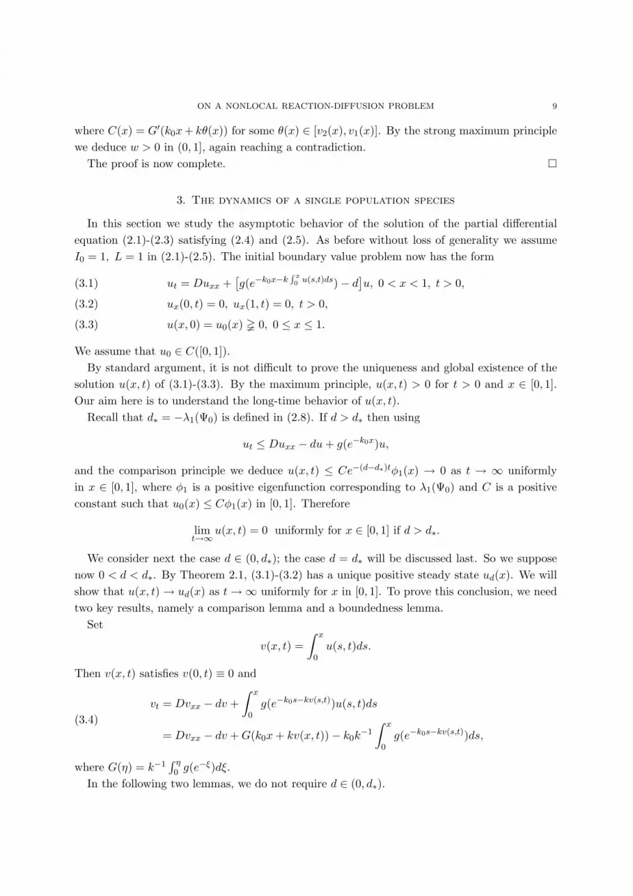
3. The dynamics of a single population species
In this section we study the asymptotic behavior of the solution of the partial differentialequation (2.1)-(2.3) satisfying (2.4) and (2.5). As before without loss of generality we assumeI0 = 1, L = 1 in (2.1)-(2.5). The initial boundary value problem now has the form
ut = Duxx +[g(e−k0x−k
∫ x0 u(s,t)ds)− d
]u, 0 < x < 1, t > 0,(3.1)
ux(0, t) = 0, ux(1, t) = 0, t > 0,(3.2)
u(x, 0) = u0(x) 0, 0 ≤ x ≤ 1.(3.3)
We assume that u0 ∈ C([0, 1]).By standard argument, it is not difficult to prove the uniqueness and global existence of the
solution u(x, t) of (3.1)-(3.3). By the maximum principle, u(x, t) > 0 for t > 0 and x ∈ [0, 1].Our aim here is to understand the long-time behavior of u(x, t).
Recall that d∗ = −λ1(Ψ0) is defined in (2.8). If d > d∗ then using
ut ≤ Duxx − du + g(e−k0x)u,
and the comparison principle we deduce u(x, t) ≤ Ce−(d−d∗)tφ1(x) → 0 as t → ∞ uniformlyin x ∈ [0, 1], where φ1 is a positive eigenfunction corresponding to λ1(Ψ0) and C is a positiveconstant such that u0(x) ≤ Cφ1(x) in [0, 1]. Therefore
limt→∞u(x, t) = 0 uniformly for x ∈ [0, 1] if d > d∗.
We consider next the case d ∈ (0, d∗); the case d = d∗ will be discussed last. So we supposenow 0 < d < d∗. By Theorem 2.1, (3.1)-(3.2) has a unique positive steady state ud(x). We willshow that u(x, t) → ud(x) as t →∞ uniformly for x in [0, 1]. To prove this conclusion, we needtwo key results, namely a comparison lemma and a boundedness lemma.
Set
v(x, t) =∫ x
0u(s, t)ds.
Then v(x, t) satisfies v(0, t) ≡ 0 and
(3.4)vt = Dvxx − dv +
∫ x
0g(e−k0s−kv(s,t))u(s, t)ds
= Dvxx − dv + G(k0x + kv(x, t))− k0k−1
∫ x
0g(e−k0s−kv(s,t))ds,
where G(η) = k−1∫ η0 g(e−ξ)dξ.
In the following two lemmas, we do not require d ∈ (0, d∗).
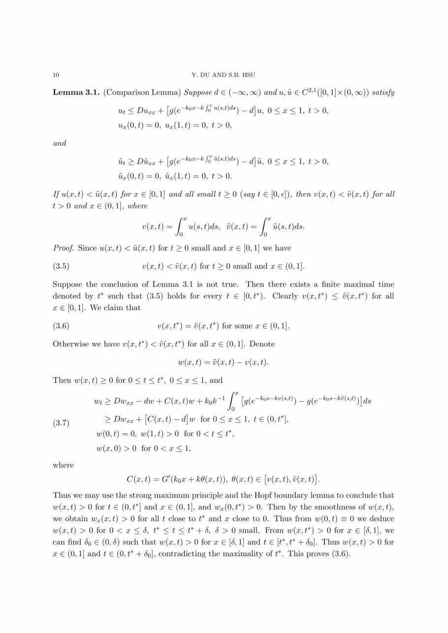
10 Y. DU AND S.B. HSU
Lemma 3.1. (Comparison Lemma) Suppose d ∈ (−∞,∞) and u, u ∈ C2,1([0, 1]×(0,∞)) satisfy
ut ≤ Duxx +[g(e−k0x−k
∫ x0 u(s,t)ds)− d
]u, 0 ≤ x ≤ 1, t > 0,
ux(0, t) = 0, ux(1, t) = 0, t > 0,
and
ut ≥ Duxx +[g(e−k0x−k
∫ x0 u(s,t)ds)− d
]u, 0 ≤ x ≤ 1, t > 0,
ux(0, t) = 0, ux(1, t) = 0, t > 0.
If u(x, t) < u(x, t) for x ∈ [0, 1] and all small t ≥ 0 (say t ∈ [0, ε]), then v(x, t) < v(x, t) for allt > 0 and x ∈ (0, 1], where
v(x, t) =∫ x
0u(s, t)ds, v(x, t) =
∫ x
0u(s, t)ds.
Proof. Since u(x, t) < u(x, t) for t ≥ 0 small and x ∈ [0, 1] we have
(3.5) v(x, t) < v(x, t) for t ≥ 0 small and x ∈ (0, 1].
Suppose the conclusion of Lemma 3.1 is not true. Then there exists a finite maximal timedenoted by t∗ such that (3.5) holds for every t ∈ [0, t∗). Clearly v(x, t∗) ≤ v(x, t∗) for allx ∈ [0, 1]. We claim that
(3.6) v(x, t∗) = v(x, t∗) for some x ∈ (0, 1].
Otherwise we have v(x, t∗) < v(x, t∗) for all x ∈ (0, 1]. Denote
w(x, t) = v(x, t)− v(x, t).
Then w(x, t) ≥ 0 for 0 ≤ t ≤ t∗, 0 ≤ x ≤ 1, and
(3.7)
wt ≥ Dwxx − dw + C(x, t)w + k0k−1
∫ x
0
[g(e−k0s−kv(s,t))− g(e−k0s−kv(s,t))
]ds
≥ Dwxx +[C(x, t)− d
]w for 0 ≤ x ≤ 1, t ∈ (0, t∗],
w(0, t) = 0, w(1, t) > 0 for 0 < t ≤ t∗,
w(x, 0) > 0 for 0 < x ≤ 1,
where
C(x, t) = G′(k0x + kθ(x, t)), θ(x, t) ∈ [v(x, t), v(x, t)
].
Thus we may use the strong maximum principle and the Hopf boundary lemma to conclude thatw(x, t) > 0 for t ∈ (0, t∗] and x ∈ (0, 1], and wx(0, t∗) > 0. Then by the smoothness of w(x, t),we obtain wx(x, t) > 0 for all t close to t∗ and x close to 0. Thus from w(0, t) ≡ 0 we deducew(x, t) > 0 for 0 < x ≤ δ, t∗ ≤ t ≤ t∗ + δ, δ > 0 small. From w(x, t∗) > 0 for x ∈ [δ, 1], wecan find δ0 ∈ (0, δ) such that w(x, t) > 0 for x ∈ [δ, 1] and t ∈ [t∗, t∗ + δ0]. Thus w(x, t) > 0 forx ∈ (0, 1] and t ∈ (0, t∗ + δ0], contradicting the maximality of t∗. This proves (3.6).

ON A NONLOCAL REACTION-DIFFUSION PROBLEM 11
Thus there exists x0 ∈ (0, 1] such that w(x0, t∗) = 0. If x0 = 1, i.e., w(1, t∗) = 0, then
wt(1, t∗) ≤ 0. By the boundary condition vxx(1, t∗) = ux(1, t∗) = 0, vxx(1, t∗) = ux(1, t∗) = 0,and hence wxx(1, t∗) = 0. Therefore we can use (3.7) to obtain
0 ≥ wt(1, t∗) ≥ k0k−1
∫ 1
0
[g(e−k0s−kv(s,t∗))− g(e−k0s−kv(s,t∗))
]ds.
Since v(x, t∗) ≤ v(x, t∗) in [0, 1], the above inequality holds only if v(x, t∗) ≡ v(x, t∗), whichimplies u(x, t∗) ≡ u(x, t∗).
From the inequality in (3.7), w(x, t) is an upper solution of the problem
wt = Dwxx − dw, 0 < x < 1, 0 < t ≤ t∗,w(0, t) = w(1, t) = 0, 0 < t ≤ t∗,w(x, 0) = w(x, 0) > 0, 0 < x < 1.
By the strong maximum principle, w(x, t) > 0 for x ∈ (0, 1) and 0 < t ≤ t∗. On the otherhand, by the comparison principle, we have w(x, t) ≥ w(x, t) for x ∈ (0, 1) and 0 < t ≤ t∗.Hence w(x, t∗) > 0 for x ∈ (0, 1). This contradicts our earlier conclusion that w(x, t∗) ≡ 0.Therefore we must have w(1, t∗) > 0. We may now apply the strong maximum principle to (3.7)to conclude that w(x, t∗) > 0 for x ∈ (0, 1], which is a contradiction to (3.6). The proof is nowcomplete. ¤
Lemma 3.2. (Boundedness Lemma) Suppose d > 0, and let u(x, t) be the unique solution of(3.1)-(3.3). Then there exists C > 0 such that
(3.8) u(x, t) ≤ C for all x ∈ [0, 1], t > 0.
Proof. Our assumption on g implies that
g(I) ≤ σI for some σ > 0 and all I ∈ [0, 1].
Therefore with
I(x, t) = exp(− k0x− k
∫ x
0u(y, t)dy
),
we have
g(I(x, t)) ≤ σI(x, t) ≤ σe−k∫ x0 udy,
and from the equation for u we deduce that
ut ≤ Duxx +[σe−k
∫ x0 udy − d
]u.
Integrating for x from 0 to 1 we obtain[ ∫ 1
0udx
]t≤ σ
∫ 1
0e−k
∫ x0 udyudx− d
∫ 1
0udx.
Denote
w(t) =∫ 1
0u(x, t)dx, v(x, t) =
∫ x
0u(y, t)dy.
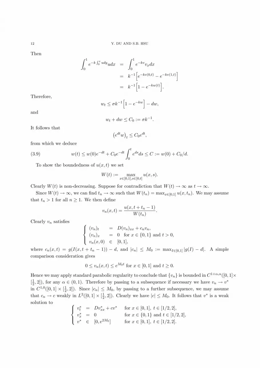
12 Y. DU AND S.B. HSU
Then∫ 1
0e−k
∫ x0 udyudx =
∫ 1
0e−kvvxdx
= k−1[e−kv(0,t) − e−kv(1,t)
]
= k−1[1− e−kw(t)
].
Therefore,wt ≤ σk−1
[1− e−kw
]− dw,
andwt + dw ≤ C0 := σk−1.
It follows that (edtw
)t≤ C0e
dt,
from which we deduce
(3.9) w(t) ≤ w(0)e−dt + C0e−dt
∫ t
0edsds ≤ C := w(0) + C0/d.
To show the boundedness of u(x, t) we set
W (t) := maxx∈[0,1],s∈[0,t]
u(x, s).
Clearly W (t) is non-decreasing. Suppose for contradiction that W (t) →∞ as t →∞.Since W (t) →∞, we can find tn →∞ such that W (tn) = maxx∈[0,1] u(x, tn). We may assume
that tn > 1 for all n ≥ 1. We then define
vn(x, t) =u(x, t + tn − 1)
W (tn).
Clearly vn satisfies
(vn)t = D(vn)xx + cnvn,
(vn)x = 0 for x ∈ 0, 1 and t > 0,
vn(x, 0) ∈ [0, 1],
where cn(x, t) = g(I(x, t + tn − 1)) − d, and |cn| ≤ M0 := maxI∈[0,1] |g(I) − d|. A simplecomparison consideration gives
0 ≤ vn(x, t) ≤ eM0t for x ∈ [0, 1] and t ≥ 0.
Hence we may apply standard parabolic regularity to conclude that vn is bounded in C1+α,α([0, 1]×[12 , 2]), for any α ∈ (0, 1). Therefore by passing to a subsequence if necessary we have vn → v∗
in C1,0([0, 1] × [12 , 2]). Since |cn| ≤ M0, by passing to a further subsequence, we may assumethat cn → c weakly in L2([0, 1]× [12 , 2]). Clearly we have |c| ≤ M0. It follows that v∗ is a weaksolution to
v∗t = Dv∗xx + cv∗ for x ∈ [0, 1], t ∈ [1/2, 2],v∗x = 0 for x ∈ 0, 1 and t ∈ [1/2, 2],v∗ ∈ [0, e2M0 ] for x ∈ [0, 1], t ∈ [1/2, 2].

ON A NONLOCAL REACTION-DIFFUSION PROBLEM 13
Since maxx∈[0,1] vn(x, 1) = 1, we have maxx∈[0,1] v∗(x, 1) = 1 and hence v∗ is not identically
zero. By the strong maximum principle we deduce v∗(x, 1) ≥ δ0 > 0 in [0, 1]. It follows thatvn(x, 1) ≥ δ0/2 for all large n and x ∈ [0, 1]. Therefore
u(x, tn) ≥ (δ0/2)W (tn) for all large n and x ∈ [0, 1].
But then we deducew(tn) ≥ (δ0/2)W (tn) →∞
as n →∞, which contradicts (3.9). Therefore there exists C > 0 such that
u(x, t) ≤ C for all x ∈ [0, 1] and t > 0.
The proof is complete. ¤
We are now ready to prove the main result of this section.
Theorem 3.3. Let 0 < d < d∗. Then the solution u(x, t) of (3.1)-(3.3) converges to the uniquesteady state ud(x) as t →∞ uniformly in x ∈ [0, 1].
Proof. We may assume that the initial data u0 satisfies u0 > 0 in [0, 1] for otherwise we canreplace u(x, t) by u(x, 1 + t) and u0(x) by u(x, 1).
Since d < d∗ = −λ1(Ψ0) and
Ψδ(x) := −g(e−(k0+kδ)x
) → Ψ0(x)
uniformly in [0, 1] as δ → 0, we can find δ > 0 sufficiently small such that d < −λ1(Ψδ). Fixsuch a δ and let φ be a positive eigenfunction corresponding to λ1(Ψδ). Then we choose ε > 0small so that εφ < u0, εφ < δ in [0, 1]. Let u(x, t) be the unique solution of (3.1)-(3.2) withinitial condition u(x, 0) = εφ(x). Then we can find σ > 0 small such that
0 < u(x, t) < δ for t ∈ (0, σ] and x ∈ [0, 1].
Hence for t ∈ (0, σ],
ut = Duxx +[g(e−k0x−k
∫ x0 u(y,t)dy
)− d]u
≥ Duxx +[−Ψδ(x)− d
]u
> Duxx +[−Ψδ(x) + λ1(Ψδ)
]u.
It follows that
(u− εφ)t > D(u− εφ)xx +[−Ψδ(x) + λ1(Ψδ)
](u− εφ), x ∈ [0, 1], t ∈ (0, σ],
(u− εφ)x = 0, x = 0, 1, t ∈ (0, σ],u− εφ = 0, x ∈ [0, 1], t = 0.
By the strong maximum principle we deduce u(x, t)− εφ(x) > 0 for t ∈ (0, σ] and x ∈ [0, 1]. Fixs ∈ (0, σ], we thus have
u(x, s) > u(x, 0) in [0, 1].
By continuity,u(x, s + t) > u(x, t) in [0, 1] for all small t ≥ 0.

14 Y. DU AND S.B. HSU
Thus we can use Lemma 3.1 to conclude that v(x, t) < v(x, s + t) for x ∈ [0, 1] and t > 0, wherev(x, t) =
∫ x0 u(s, t)ds. It follows that v(x, t) is monotone increasing in t.
By Lemma 3.2, v(x, t) ≤ C for all x ∈ [0, 1] and t > 0 for some C > 0. Hence limt→∞ v(x, t) =v∗(x) exists. On the other hand, due to the boundedness of ‖u(·, t)‖∞ (which follows fromLemma 3.2), we can apply the standard parabolic regularity theory to (3.1)-(3.2) to concludethat, for any sequence tn → ∞, u(·, tn) has a subsequence which converges in C1([0, 1]), sayu(·, tnk
) → u∗. Since v(·, tn) → v∗, we necessarily have v∗(x) =∫ x0 u∗(y)dy. Hence u∗ = v′∗. This
implies that limt→∞ u(x, t) exists and equals v′∗(x). It follows that v′∗ must be a nonnegativesteady state of (3.1), (3.2). Since v∗(0) = 0 and v∗ is the limit of an increasing sequence, wehave v∗(x) > 0 for x ∈ (0, 1] and v′∗ 6≡ 0. Therefore v′∗ is a nontrivial nonnegative steady stateof (3.1), (3.2). By the strong maximum principle v′∗ is positive and hence we can use Theorem2.1 to conclude that v′∗ ≡ ud.
Next we consider dM = −λ1
(ΨM )
)with M > 0 large. Recall that ΨM (x) = −g
(e−(k0+kM)x
).
Let φM (x) be the positive eigenfunction corresponding to λ1(ΨM ) with ‖φM‖∞ = 1. It is easyto see by a regularity and compactness argument that as M →∞, λ1(ΨM ) → 0 and φM → 1 inC1([0, 1]). Therefore we can find M0 > 0 large so that
d > −λ1(ΨM ),12
< φM (x) ≤ 1 for M ≥ M0.
We now fix M > M0 such that 2M > u0(x) in [0, 1]. Then
u0(x) < 2MφM (x) and M < 2MφM (x) for x ∈ [0, 1].
Let u(x, t) be the solution of (3.1)-(3.2) with initial condition u(x, 0) = 2MφM (x). Then we canfind δ0 > 0 small so that u0(x) < u(x, t), M < u(x, t) for t ∈ (0, δ0] and x ∈ [0, 1]. Hence fort ∈ (0, δ0], we have
ut = Duxx +[g(e−k0x−k
∫ x0 u(y,t)dy
)− d]u
≤ Duxx +[−ΨM (x)− d
]u
< Duxx +[−ΨM (x) + λ1(ΨM )
]u.
Thus for w(x, t) := u(x, t)− 2MφM (x), we have
wt < Dwxx +[−ΨM (x) + λ1(ΨM )
]w, x ∈ [0, 1], t ∈ (0, δ0],
wx = 0, x = 0, 1, t ∈ (0, δ0],w = 0, x ∈ [0, 1], t = 0.
By the strong maximum principle we deduce w = u − 2MφM < 0 for t ∈ (0, δ0] and x ∈ [0, 1].It follows that u(x, s) < u(x, 0) for 0 < s ≤ δ0. Using the same argument as before, we deducethat
v(x, t) :=∫ x
0u(s, t)ds
is monotone decreasing in t. Moreover, from Lemma 3.1 it follows that v(x, t) > v(x, t) :=∫ x0 u(s, t)ds > v(x, t) for all t > 0 and x ∈ (0, 1]. Hence limt→∞ v(x, t) = v∗(x) ≥ ∫ x
0 ud(s)ds.We may then use parabolic regularity theory much as before to deduce that u(x, t) → (v∗)′(x)

ON A NONLOCAL REACTION-DIFFUSION PROBLEM 15
in C1([0, 1]), and (v∗)′(x) is a positive steady state of (3.1)-(3.2). Thus we must have (v∗)′(x) ≡ud(x).
Since v ≤ v ≤ v, and limt→∞ v(x, t) = limt→∞ v(x, t) =∫ x0 ud(s)ds, we necessarily have
limt→∞ v(x, t) =
∫ x
0ud(s)ds.
Thus we can repeat the above argument to conclude that u(x, t) → ud(x) as t → ∞ uniformlyfor x ∈ [0, 1]. This completes the proof. ¤
Finally we consider the case d = d∗.
Theorem 3.4. Suppose d = d∗. Then the solution u(x, t) to (3.1)-(3.3) converges to 0 as t →∞uniformly in x ∈ [0, 1].
Proof. This follows from a simple modification of the second part of the proof of Theorem 3.3.Indeed, let u(x, t) be defined exactly as in the proof of Theorem 3.3. Then we know thatv(x, t) :=
∫ x0 u(s, t)ds > 0 is strictly decreasing in t. Hence limt→∞ v(x, t) = v∗(x) ≥ 0 exists.
By the same consideration as in the proof of Theorem 3.3 we can show that u(x, t) → (v∗)′(x) ast →∞ in the norm of C1([0, 1]), and hence (v∗)′(x) is a nonnegative steady-state of (3.1)-(3.2).However, since d = d∗, by Theorem 2.1, the only nonnegative steady state of (3.1)-(3.2) is thetrivial solution 0. Hence u(x, t) → 0 as t → ∞ uniformly for x ∈ [0, 1], and thus v(x, t) → 0 ast →∞.
Using Lemma 3.1 we deduce 0 < v(x, t) < v(x, t), which implies that v(x, t) → 0 as t → ∞.Using this fact and the parabolic regularity, as before, we deduce limt→∞ u(·, t) exists in theC1([0, 1]) norm, and the limit is a nonnegative steady state of (3.1)-(3.2). Since d = d∗, thislimit must be 0. This completes the proof. ¤
4. Steady-states of the two species model
In this section we study the steady-states of the system (1.1)-(1.3) with n = 2. As before weassume, without loss of generality, L = 1 and I0 = 1. Thus we are interested in the nonnegativesolutions of the elliptic system
(4.1)
D1(u1)xx +[g1(I(x))− d1
]u1 = 0, 0 < x < 1,
D2(u2)xx +[g2(I(x))− d2
]u2 = 0, 0 < x < 1,
(ui)x(0) = (ui)x(1) = 0, i = 1, 2,
where g1(I), g2(I) satisfy (2.4), and
I(x) = e−k0x exp(−
∫ x
0
[k1u1(y) + k2u2(y)
]dy
),
with k0, k1, k2 > 0.In the following we will regard k0, k1, k2 as fixed constants and treat d1 and d2 as varying
parameters. We need to introduce some notations first. We will use λ1(Ψ) to denote the first

16 Y. DU AND S.B. HSU
eigenvalue of (2.7) with D = D1 and use µ1(Ψ) to denote the first eigenvalue of (2.7) withD = D2. We also denote
d∗1 = −λ1(−g1(e−k0x)), d∗2 = −µ1(−g2(e−k0x)).
Nonnegative solutions of (4.1) can be classified into three classes: The unique trivial solution(u1, u2) ≡ (0, 0), which exists for all d1 and d2. Two semitrivial solutions (u1, u2) = (0, u∗d2
) and(u1, u2) = (u∗d1
, 0), the former exists for d2 ∈ (0, d∗2) and the latter exists for d1 ∈ (0, d∗1), whereu∗d1
, d∗d2denote the unique steady state for the u1 and u2 equations, respectively, guaranteed by
Theorem 2.1. The third class are positive solutions (u1, u2) with u1(x) > 0 and u2(x) > 0 in[0, 1], which are the most difficult to understand and are the main interest here.
Some necessary conditions for the existence of a positive solution to (4.1) can be easily ob-served. Suppose that (u1, u2) is a positive solution of (4.1). Then from the equation for u1 weobtain
−d1 = λ1(−g1(e−k0x−∫ x0 (k1u1+k2u2)dy)) ∈ (λ1(−g1(e−k0x)), λ1(0)) = (−d∗1, 0).
That is d1 ∈ (0, d∗1). Similarly from the equation for u2 we deduce d2 ∈ (0, d∗2). Thus for (4.1)to possess a positive solution we necessarily have
(4.2) 0 < d1 < d∗1, 0 < d2 < d∗2.
Next we assume (4.2) and use a global bifurcation argument to find sufficient conditions forthe existence of positive solutions to (4.1). We will rewrite (4.1) as an abstract equation involvinga completely continuous operator. Let E = C([0, 1]) and let P be the usual positive cone in E:P = u ∈ E : u(x) ≥ 0 in [0, 1]. We define A : E ×E → E × E by
A(u1, u2) = (A1(u1, u2), A2(u1, u2)),
whereA1(u1, u2) = L1 G1(d1, u1, u2), A2(u1, u2) = L2 G2(d2, u1, u2),
G1(d1, u1, u2)(x) =[d∗1 − d1 + g1(e−k0x−∫ x
0 (k1u1+k2u2)dy)]u1(x),
G2(d2, u1, u2)(x) =[d∗2 − d2 + g2(e−k0x−∫ x
0 (k1u1+k2u2)dy)]u2(x),
and for i = 1, 2, Li is the solution operator for the problem
−Diuxx + d∗i u = fi(x), ux(0) = ux(1) = 0,
namely u = Li(fi). It is easily seen that (u1, u2) solves (4.1) if and only if (u1, u2) = A(u1, u2).By standard elliptic regularity theory we know that A : E × E → E × E is completely
continuous. Moreover, by the strong maximum principle and the fact that (due to (4.2))
d∗i − di + gi(e−k0x−∫ x0 (k1u1+k2u2)dy) > 0 in [0, 1],
we find that if ui ∈ P then Ai(u1, u2) ∈ P , and if ui ∈ P := P \ 0 then Ai(u1, u2) ∈ P :=u ∈ P : u(x) > 0 in [0, 1]. Thus we have
A(P × P ) ⊂ P × P, A(P × P ) ⊂ P × P ,
A(P × P ) ⊂ P × P, A(P × P ) ⊂ P × P .
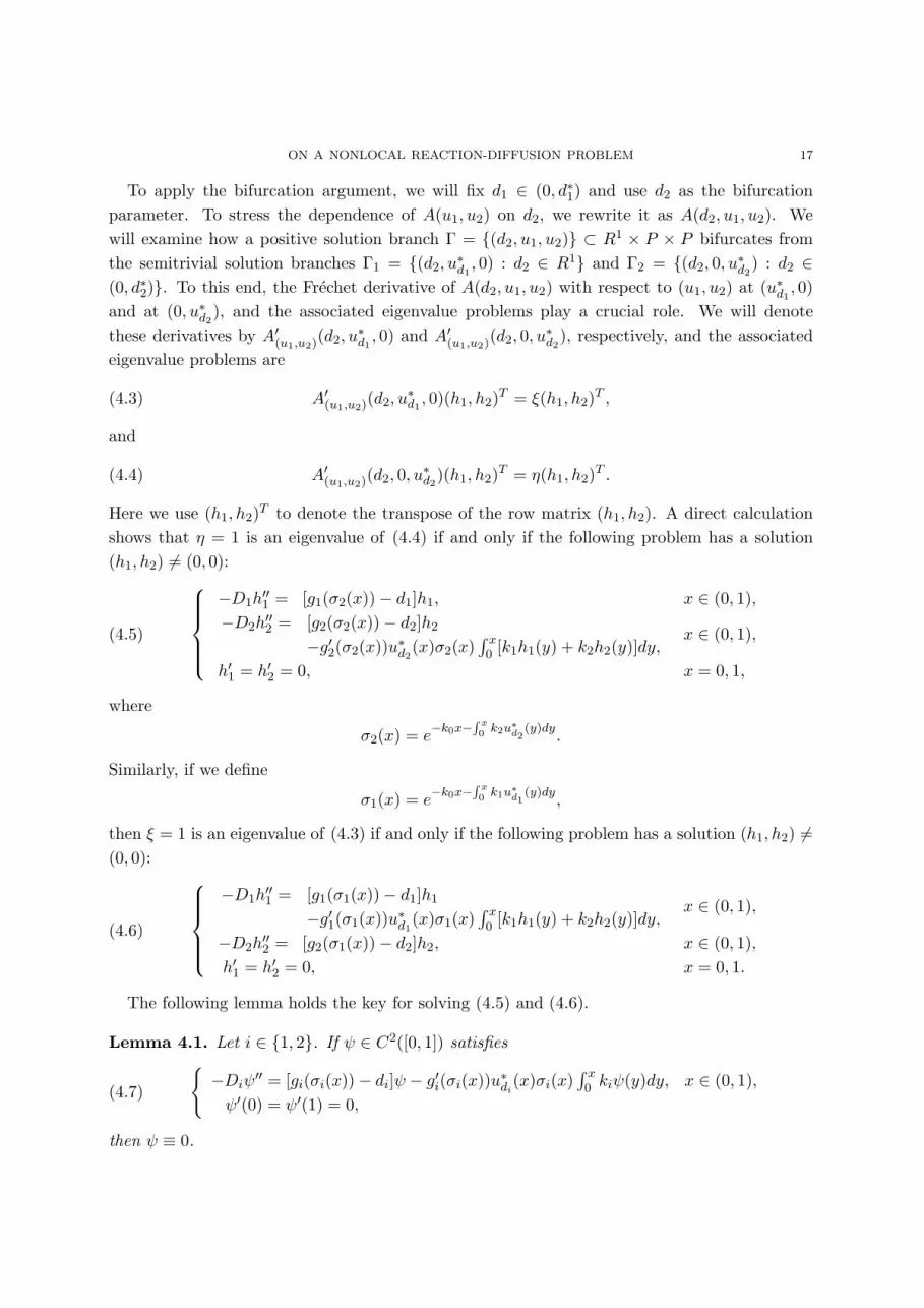
ON A NONLOCAL REACTION-DIFFUSION PROBLEM 17
To apply the bifurcation argument, we will fix d1 ∈ (0, d∗1) and use d2 as the bifurcationparameter. To stress the dependence of A(u1, u2) on d2, we rewrite it as A(d2, u1, u2). Wewill examine how a positive solution branch Γ = (d2, u1, u2) ⊂ R1 × P × P bifurcates fromthe semitrivial solution branches Γ1 = (d2, u
∗d1
, 0) : d2 ∈ R1 and Γ2 = (d2, 0, u∗d2) : d2 ∈
(0, d∗2). To this end, the Frechet derivative of A(d2, u1, u2) with respect to (u1, u2) at (u∗d1, 0)
and at (0, u∗d2), and the associated eigenvalue problems play a crucial role. We will denote
these derivatives by A′(u1,u2)(d2, u∗d1
, 0) and A′(u1,u2)(d2, 0, u∗d2), respectively, and the associated
eigenvalue problems are
(4.3) A′(u1,u2)(d2, u∗d1
, 0)(h1, h2)T = ξ(h1, h2)T ,
and
(4.4) A′(u1,u2)(d2, 0, u∗d2)(h1, h2)T = η(h1, h2)T .
Here we use (h1, h2)T to denote the transpose of the row matrix (h1, h2). A direct calculationshows that η = 1 is an eigenvalue of (4.4) if and only if the following problem has a solution(h1, h2) 6= (0, 0):
(4.5)
−D1h′′1 = [g1(σ2(x))− d1]h1, x ∈ (0, 1),
−D2h′′2 = [g2(σ2(x))− d2]h2
−g′2(σ2(x))u∗d2(x)σ2(x)
∫ x0 [k1h1(y) + k2h2(y)]dy,
x ∈ (0, 1),
h′1 = h′2 = 0, x = 0, 1,
where
σ2(x) = e−k0x−∫ x
0 k2u∗d2(y)dy
.
Similarly, if we define
σ1(x) = e−k0x−∫ x
0 k1u∗d1(y)dy
,
then ξ = 1 is an eigenvalue of (4.3) if and only if the following problem has a solution (h1, h2) 6=(0, 0):
(4.6)
−D1h′′1 = [g1(σ1(x))− d1]h1
−g′1(σ1(x))u∗d1(x)σ1(x)
∫ x0 [k1h1(y) + k2h2(y)]dy,
x ∈ (0, 1),
−D2h′′2 = [g2(σ1(x))− d2]h2, x ∈ (0, 1),
h′1 = h′2 = 0, x = 0, 1.
The following lemma holds the key for solving (4.5) and (4.6).
Lemma 4.1. Let i ∈ 1, 2. If ψ ∈ C2([0, 1]) satisfies
(4.7)
−Diψ
′′ = [gi(σi(x))− di]ψ − g′i(σi(x))u∗di(x)σi(x)
∫ x0 kiψ(y)dy, x ∈ (0, 1),
ψ′(0) = ψ′(1) = 0,
then ψ ≡ 0.

18 Y. DU AND S.B. HSU
Proof. We argue indirectly. Suppose ψ 6≡ 0 solves (4.7). We first claim that ψ(0) 6= 0. Otherwise,define
ξ(x) =∫ x
0ψ(y)dy, η(x) = ψ′(x).
Then (ξ(x), ψ(x), η(x)) is a solution of the ODE system
ξ′ = ψ,
ψ′ = η,
η′ = −D−1i [gi(σi(x))− di]ψ + D−1
i g′i(σi(x))u∗di(x)σi(x)kiξ,
with initial condition (ξ(0), ψ(0), η(0)) = (0, 0, 0). Clearly (ξ, ψ, η) ≡ (0, 0, 0) is the uniquesolution of this initial value ODE problem. Hence ψ ≡ 0, contradicting our assumption thatψ 6≡ 0. This proves our claim that ψ(0) 6= 0.
Without loss of generality we may assume that ψ(0) > 0. Next we claim that ψ(x) changessign in (0, 1). Otherwise ψ(x) ≥, 6≡ 0 in [0, 1]. Multiply the first equation in (4.7) by u∗di
andintegrate it over [0, 1]; we easily deduce
∫ 1
0
(g′i(σi(x))[u∗di
(x)]2σi(x)∫ x
0kiψ(y)dy
)dx = 0.
But the integrand function of x is clearly nonnegative and not identically zero in [0, 1]. Hencethe integral should be positive. This contradiction shows that ψ(x) changes sign in (0, 1).
Let x0 ∈ (0, 1) be the first zero of ψ(x), namely ψ(x) > 0 in [0, x0) and ψ(x0) = 0. We nowconsider the eigenvalue problem
(4.8) −Diφ′′ = [gi(σi(x))− di]φ + λφ in (0, x0), φ′(0) = φ(x0) = 0.
We claim that the first eigenvalue λ1 of this problem is positive. Indeed, let φ1 be a positiveeigenfunction corresponding to λ1. By the Hopf boundary lemma, φ′1(x0) < 0. Multiplying thefirst equation in (4.8) (with λ = λ1, φ = φ1) by u∗di
and integrating over [0, x0] we obtain∫ x0
0[gi(σi)− di]φ1u
∗di
+ λ1
∫ x0
0φ1u
∗di
= −Di
∫ x0
0φ′′1u
∗di
= −Diφ′1(x0)u∗di
(x0)−Di
∫ x0
0(u∗di
)′′φ1
>
∫ x0
0[gi(σi)− di]φ1u
∗di
.
Hence λ1
∫ x0
0 φ1u∗di
> 0, which gives λ1 > 0, as claimed.To obtain the desired contradiction, we now multiply the first equation in (4.8) (with λ =
λ1, φ = φ1) by ψ and then integrate it over [0, x0]. It results∫ x0
0[gi(σi)− di]φ1ψ + λ1
∫ x0
0φ1ψ
= −Di
∫ x0
0φ′′1ψ = −Di
∫ x0
0ψ′′φ1
=∫ x0
0[gi(σi)− di]φ1ψ −
∫ x0
0
[g′i(σi)σiu
∗di
∫ x
0kiψdy
]φ1dx.

ON A NONLOCAL REACTION-DIFFUSION PROBLEM 19
It follows that
(4.9) λ1
∫ x0
0φ1ψ = −
∫ x0
0
[g′i(σi)σiu
∗di
∫ x
0kiψdy
]φ1dx.
Since λ1 > 0 and ψ(x) > 0 in [0, x0), the left side of the above identity is positive. However, thebracketed integrand function in the right side of (4.9) is nonnegative and hence the right side of(4.9) is not positive. This contradiction completes the proof. ¤
Using Lemma 4.1, we can easily prove the following result.
Lemma 4.2. Problem (4.5) has a solution (h1, h2) 6= (0, 0) if and only if h1 6= 0 and
−D1h′′1 = [g1(σ2(x))− d1]h1, h′1(0) = h′1(1) = 0.
Moreover, with h1 given, h2 can be uniquely solved from the second equation in (4.5) togetherwith the Neumann boundary conditions.
Similarly, (4.6) has a solution (h1, h2) 6= (0, 0) if and only if h2 6= 0 and
−D2h′′2 = [g2(σ1(x))− d2]h2, h′2(0) = h′2(1) = 0.
Moreover, with h2 given, h1 can be uniquely solved from the first equation in (4.6) together withthe Neumann boundary conditions.
Proof. We only consider the statement for (4.5); the proof of that for (4.6) is analogous. Let(h1, h2) solve (4.5). If h1 = 0, then by Lemma 4.1 we deduce h2 = 0. Suppose now h1 6= 0.Then we can apply the Fredholm alternative for compact operators and Lemma 4.1 to concludethat the second equation in (4.5) together with the Neumann boundary conditions is uniquelysolvable for any given h1. ¤
Recall thatσ2(x) = σ2(d2, x) = e
−k0x−∫ x0 k2u∗d2
(y)dy,
andσ1(x) = σ1(d1, x) = e
−k0x−∫ x0 k1u∗d1
(y)dy.
By Theorem 2.1 (iv), we know that d2 → σ2(d2, x) is strictly increasing for x ∈ (0, 1]. Thisimplies that
λ(d2) := −λ1
(− g1(σ2(d2, ·)))
is strictly increasing for d2 ∈ (0, d∗2). By Theorem 2.1 (i), we know that λ(d2) is continuous.Since u∗d2
(x) → 0 uniformly in [0, 1] as d2 → d∗2 and u∗d2(x) → ∞ uniformly in [0, 1] as d2 → 0,
we easily see thatlim
d2→0λ(d2) = 0, lim
d2→d∗2λ(d2) = d∗1.
Therefore for any given d1 ∈ (0, d∗1), there exists a unique d2 = d2(d1) ∈ (0, d∗1) such that
(4.10) λ(d2) = d1.
Let us also introduce
(4.11) d2 = d2(d1) := −µ1
(− g2(σ1(d1, ·))).

20 Y. DU AND S.B. HSU
It is easily seen that d2 ∈ (0, d∗2).We are now ready to state and prove our main result of this section.
Theorem 4.3. For fixed d1 ∈ (0, d∗1) let d2 and d2 be defined as above. Then (4.1) has a positivesolution (u1, u2) if d2 lies between d2 and d2. Moreover, there exists a branch of positive solutionsΓ = (d2, u1, u2) ⊂ R1 × E × E that meets the semitrivial solution branch Γ1 = (d2, u
∗d1
, 0) :d2 ∈ R1 precisely at (d2, u
∗d1
, 0), and meets the semitrivial solution branch Γ2 = (d2, 0, u∗d2) :
d2 ∈ (0, d∗2) precisely at (d2, 0, u∗d2
). More accurately, Γ is a connected set in R1 × E × E such
that Γ ∩ Γ1 = (d2, u∗d1
, 0), Γ ∩ Γ2 = (d2, 0, u∗d2
), and Γ \ (d2, u∗d1
, 0), (d2, 0, u∗d2
) consists ofpositive solutions of (4.1).
Proof. For clarity we divide the proof into four steps.Step 1: We show that for any small δ > 0 and fixed d1 ∈ (0, d∗1), there exists C such that anypositive solution (u1, u2) of (4.1) with d2 ∈ [δ, d∗2 − δ] satisfies
(4.12) ‖u1‖∞ + ‖u2‖∞ < C.
Otherwise we can find a small δ > 0 and a sequence dn2 ∈ [δ, d∗2− δ] such that (4.1) with d2 = dn
2
has a positive solution (un1 , un
2 ) satisfying
limn→∞(‖un
1‖∞ + ‖un2‖∞) = ∞.
By passing to a subsequence, we have either ‖un2‖∞ →∞ or ‖un
1‖∞ →∞. In the first case, wedefine un = un
2/‖un2‖∞. Then from the equation for un
2 we deduce
(4.13) −D2u′′n =
[g2(fn(x))− dn
2 ]un, u′n(0) = u′n(1) = 0,
wherefn(x) = e−k0x−∫ x
0 (k1un1 +k2un
2 )dy.
Since ‖un‖∞ = 1 and the right side of the first equation in (4.13) has a bound in L∞([0, 1])that is independent of n, by standard elliptic regularity we know that un is precompact inC1([0, 1]). Hence by passing to a subsequence we may assume that un → u in C1([0, 1]). Since0 < fn(x) ≤ 1 and δ ≤ dn
2 ≤ d∗2 − δ, by passing to a subsequence we may assume that fn → f
weakly in L2([0, 1]) and dn2 → d∞2 , with 0 ≤ f ≤ 1 and d∞2 ∈ [δ, d∗2− δ]. Since g2 is C1, we easily
see that g2(fn) → g2(f) weakly in L2([0, 1]). Thus u is a weak solution to
−D2u′′ = [g2(f(x))− d∞2 ]u, u′(0) = u′(1) = 0.
Clearly u ≥ 0 and ‖u‖∞ = 1. Thus we can apply the strong maximum principle to conclude thatu(x) > 0 in [0, 1]. This implies that un
2 (x) →∞ uniformly in [0, 1] and hence f ≡ 0, g2(f) ≡ 0.Thus u is a positive solution of
−D2u′′ = −d∞2 u, u′(0) = u′(1) = 0.
This implies that −d∞2 = µ1(0) = 0, a contradiction to d∞2 ∈ [δ, d∗2 − δ].If ‖un
1‖∞ → ∞, then we can use the equation for un1 and a similar argument to reach a
contradiction. This completes the proof of Step 1.
ON A NONLOCAL REACTION-DIFFUSION PROBLEM 21
Step 2: We show that if δ > 0 is small enough, then (4.1) has no positive solution if d2 6∈(δ, d∗2 − δ).
Otherwise, due to (4.2), we can find dn2 ↓ 0 or dn
2 ↑ d∗2 and a positive solution (un1 , un
2 ) of (4.1)with d2 = dn
2 . In the first case we define un and fn as in Step 1 above, and find by the samereasoning that by passing to a subsequence un → u in C1([0, 1]), fn → f and g2(fn) → g2(f)weakly in L2([0, 1]), and u is a positive solution to
−D2u′′ = g2(f)u, u′(0) = u′(1) = 0.
Integrating the first equation for x over [0, 1], we deduce∫ 10 g2(f)udx = 0. Since u > 0 in [0, 1]
and g2(f(x)) ≥ 0 in [0, 1], the above identity implies that g2(f(x)) = 0 a.e. in [0, 1]. It followsthat f(x) = 0 a.e. in [0, 1].
Now define vn = un1/‖un
1‖∞ and we obtain from the equation for un1 that
−D1vn = [g1(fn(x))− d1]vn, v′n(0) = v′n(1) = 0.
As before by elliptic regularity, subject to passing to a subsequence, vn → v in C1([0, 1]) andg2(fn) → g1(f) = 0 weakly in L2([0, 1]), and v is a positive solution to
−D1v′′ = −d1v, v′(0) = v′(1) = 0.
This implies d1 = 0, a contradiction to our assumption d1 ∈ (0, d∗1).Next we consider the case dn
2 → d∗2. We define un, vn and fn as above. By the same argumentwe know that by passing to a subsequence, un → u and vn → v in C1([0, 1]), fn → f andgi(fn) → gi(f) weakly in L2([0, 1]), and u, v are positive solutions to
(4.14) −D2u′′ = [g2(f)− d∗2]u, u′(0) = u′(1) = 0,
and
(4.15) −D1v′′ = [g1(f)− d1]v, v′(0) = v′(1) = 0,
respectively.Let us now look at the sequence ‖un
1‖∞. If this sequence is not bounded, then by passingto a subsequence we have ‖un
1‖∞ →∞ and hence un1 = ‖un
1‖∞vn →∞ uniformly in [0, 1]. Thisimplies that f ≡ 0 and hence (4.15) becomes
−D1v′′ = −d1v, v′(0) = v′(1) = 0,
which implies d1 = 0, a contradiction. Thus ‖un1‖∞ is bounded. For the same reason, ‖un
2‖∞is bounded. So we may assume that
‖un1‖∞ → α1 ≥ 0, ‖un
2‖∞ → α2 ≥ 0.
It then follows that
fn(x) → e−k0x−∫ x0 (k1α1v+k2α2u)dy uniformly in [0, 1].
Thusf(x) = e−k0x−∫ x
0 (k1α1v+k2α2u)dy ≤ e−k0x

22 Y. DU AND S.B. HSU
with equality holding for all x ∈ [0, 1] if and only if α1 = α2 = 0. It follows that g2(f(x)) ≤g2(e−k0x) with equality holding for all x ∈ [0, 1] if and only if α1 = α2 = 0. From this and (4.14)we deduce
d∗2 = −µ1(−g2(f)) ≤ −µ1(−g2(e−k0x)),
with equality holding if and only if α1 = α2 = 0. Thus in view of the definition of d∗2, wenecessarily have α1 = α2 = 0 and thus f(x) = e−k0x. We now use (4.15) and find
d1 = −λ1(−g1(f)) = −λ1(−g1(e−k0x)).
That is, d1 = d∗1, a contradiction to our assumption on d1. This completes our proof of Step 2.Step 3: Global bifurcation analysis.
Let us now fix δ > 0 small enough such that (4.1) has no positive solution for d2 6∈ Λ :=(δ, d∗2 − δ), and d2, d2 ∈ Λ. Then define Ω = Λ× U × V with
U = u1 ∈ P : ‖u1‖∞ < C, V = u2 ∈ P : ‖u2‖∞ < C,
where C > 0 is large enough such that (4.12) holds and ‖u∗d1‖∞ < C.
We are going to apply the global bifurcation result of [5], namely Theorem 2.3 in [5], to theoperator
(d2, u1, u2) ∈ Ω → A(d2, u1, u2) ∈ P × P.
It is easily seen that the conditions (I′), (II′) and (III′) in that theorem are satisfied, withT = (u∗d1
, 0). By that theorem, if for some small ε > 0, A(d2, u1, u2) = (u1, u2) has nobifurcation value in (d2 − ε, d2) ∪ (d2, d2 + ε), and
(4.16) indexP×P (A(λ, ·), (u∗d1, 0)) 6= indexP×P (A(µ, ·), (u∗d1
, 0))
for λ ∈ (d2 − ε, d2), µ ∈ (d2, d2 + ε), then
(i) d2 = d2 is a bifurcation value,(ii) there is a connected set Σ ⊂ Σ∗, where Σ∗ = (d2, u1, u2) ∈ Ω : A(d2, u1, u2) =
(u1, u2), u2 6= 0, such that Σ contains the point (d2, u∗d1
, 0) and(a) a point (λ0, u
∗d1
, 0) with λ0 6= d2, or(b) a point in ∂Ω, or(c) a point in Λ× (0, 0).
where
∂Ω := (d2, u1, u2) ∈ Ω : d2 = δ, or d2 = d∗2 − δ, or ‖u1‖∞ = C, or ‖u2‖∞ = C.
By Lemma 4.2 we find that for ε > 0 small and d2 ∈ [d2 − ε, d2 + ε] \ d2, (u∗d1, 0) is a
nondegenerate solution of (4.1). Thus there is no bifurcation value in [d1 − ε, d2 + ε] \ d2. Itfollows that the fixed point indices (with respect to the cone P × P ) in (4.16) are well-definedand are independent of λ and µ in their respective given ranges.
Suppose for the moment that (4.16) holds; we now analyze the connected set Σ. We firstobserve that Σ ∩ Γ1 = (d2, u
∗d1
, 0). Indeed, suppose (λ, u∗d1, 0) ∈ Σ ∩ Γ1. Then we can find

ON A NONLOCAL REACTION-DIFFUSION PROBLEM 23
a sequence of points (dn2 , un
1 , un2 ) ∈ Σ∗ that converges to (λ, u∗d1
, 0) in R1 × E × E. Using theequation for un
2 we obtain
−dn2 = µ1(−g2(e−k0x−∫ x
0 (k1un1 +k2un
2 )dy)) → µ1(−g2(e−k0x−∫ x
0 k1u∗d1dy)) = −d2.
Hence λ = d2. This proves Σ ∩ Γ1 = (d2, u∗d1
, 0), which implies that alternative (a) cannotoccur.
We now show that alternative (c) does not happen either. Otherwise, we can find a sequenceof points (dn
2 , un1 , un
2 ) ∈ Σ∗ that converges to (λ, 0, 0) ∈ Λ× (0, 0). Again we use the equation forun
2 and obtain
−dn2 = µ1(−g2(e−k0x−∫ x
0 (k1un1 +k2un
2 )dy)) → µ1(−g2(e−k0x)) = −d∗2.
Thus d∗2 = λ ∈ Λ = (δ, d∗2 − δ), which is a contradiction. Hence (c) cannot occur.So alternative (b) necessarily happens. But by our choice of δ and C used in the definition of
Ω, no positive solution (d2, u1, u2) belongs to ∂Ω. Thus necessarily Σ∩∂Ω consists of semitrivialsolutions. Since Σ ∩ Γ1 = (d2, u
∗d1
, 0) and d2 ∈ Λ, ‖u∗d1‖∞ < C, the semitrivial solutions in
Σ ∩ ∂Ω must belong to Γ2. This shows that Σ intersects Γ2.We show next that Σ has a subset Γ which is connected and has the following properties:
Γ ∩ Γ2 = (d2, 0, u∗d2
), Γ ∩ Γ1 = (d2, u∗d1
, 0),
Γ \ (d2, u∗d1
, 0), (d2, 0, u∗d2
) consists of positive solutions of (4.1).
To this end we consider Γ∗ := Σ\Γ2. By what was proved above, we know that (d2, u∗d1
, 0) ∈ Γ∗.From the connectedness of Σ we easily deduce that Γ∗ ∩ Γ2 6= ∅. Then much as before wecan show that Γ∗ ∩ Γ2 = (d2, 0, u∗
d2). We claim that Γ∗ has a connected component Γ which
contains both (d2, 0, u∗d2
) and (d2, u∗d1
, 0). Otherwise, let Γ1∗ be the maximal connected subset
of Γ∗ containing (d2, u∗d1
, 0); then Γ1∗ and Σ \ Γ1∗ have positive distance to each other, whichimplies that Σ is not connected. This proves that the above mentioned Γ does exist. Much asbefore we can easily show that Γ∩Γ2 = (d2, 0, u∗
d2) and Γ∩Γ1 = (d2, u
∗d1
, 0). It follows that
Γ \ (d2, u∗d1
, 0), (d2, 0, u∗d2
) consists of positive solutions of (4.1).To complete the proof of the theorem, it remains to prove (4.16).
Step 4: Fixed point index calculation.We now calculate the fixed point indices appearing in (4.16) by making use of Theorem 2.1 in
[4]. Let B1 be a small ball in E containing u∗d1. Since u∗d1
∈ P , we may assume that B1 ⊂ P .Then by Theorem 2.1 of [4], we have
indexP×P (A(d2, ·), (u∗d1, 0)) =
0 if r(L) > 1,
degP (I −A1(·, 0), B1) if r(L) < 1,
where L = (A2)′u2(u∗d1
, 0) and r(L) denotes the spectral radius of the linear operator L.

24 Y. DU AND S.B. HSU
It is easily checked that r(L) > 1 if d2 < −µ1(−g2(σ1)) = d2, and r(L) < 1 if d2 >
−µ1(−g2(σ1)) = d2. Thus
indexP×P (A(d2, ·), (u∗d1, 0)) =
0 if d2 < d2,
degP (I −A1(·, 0), B1) if d2 > d2.
We show next that
degP (I −A1(·, 0), B1) = 1.
Since u∗d1is the only fixed point of A1(·, 0) in B1, we clearly have
degP (I −A1(·, 0), B1) = indexP (A1(·, 0), u∗d1).
We will use a homotopy argument to A1(λ, u1, 0) = L1 G1(λ, u1, 0) with λ ∈ [d1, d∗1 + 1]. By
Theorem 2.1 we know that for λ ∈ [d1, d∗1) the equation A1(λ, u, 0) = u has exactly two solutions
in P : The trivial solution u = 0 and the unique positive solution u = uλ > 0. For λ ∈ [d∗1, d∗1+1],
there is one solution in P : u = 0. Moreover, one easily sees that 0 is a linearized stable fixedpoint of A1(λ, ·, 0) when λ > d∗1, and it is a linearized unstable fixed point when λ < d∗1. Itfollows that
indexP (A1(λ, ·, 0), 0) = 0 for λ < d∗1 and this index is 1 for λ > d∗1.
Choose C0 > 0 large enough such that ‖uλ‖∞ < C0 for λ ∈ [d1, d∗1), and denote PC0 := u ∈ P :
‖u‖∞ < C0. Then by the homotopy invariance property of the topological degree, we find thatdegP (I − A(λ, ·, 0), PC0) is well-defined and its value does not depend on λ for λ ∈ [d1, d
∗1 + 1].
By the additivity of the topological degree we have
degP (I −A1(λ, ·, 0), PC0) = indexP (A1(λ, ·, 0), 0) + indexP (A1(λ, ·, 0), uλ)= indexP (A1(λ, ·, 0), uλ)
for λ ∈ [d1, d∗1), and
degP (I −A(λ, ·, 0), PC0) = indexP (A1(λ, ·, 0), 0) = 1
for λ ∈ (d∗1, d∗1 + 1]. It follows that
indexP (A1(λ, ·, 0), uλ) = 1
for λ ∈ [d1, d∗1). Taking λ = d1 we obtain
degP (I −A1(·, 0), B1) = indexP (A1(·, 0), u∗d1) = 1.
Thus (4.16) holds, and the proof is complete. ¤
Remark 4.4. The degree calculation methods developed in [4, 6] and the bifurcation method of[5] can also be used to study the existence of positive steady states of the phytoplankton modelwith three and more species.

ON A NONLOCAL REACTION-DIFFUSION PROBLEM 25
We note that the global bifurcation arguments in [2] do not seem easily applicable to ourproblem here. Firstly in the abstract global bifurcation result in [2] the fixed point index inthe entire space is required, which was calculated there based on a good understanding of theeigenvalues of (4.3) with ξ 6= 1. This seems difficult to obtain due to the nonlocal terms inour problem. Secondly the analysis in [2] also relies on the local bifurcation result of [3], whichrequires the bifurcation point to correspond to a simple eigenvalue. In contrast, the globalbifurcation result of [5] used here involves the fixed point index in the positive cone, whichdepends on (4.3) with ξ = 1 and the second equation in (4.6), which are much easier to handle.Moreover, the result of [5] can be used to discuss systems with more than two equations. (Thefixed point index calculation in [2] can also be done by using Theorem 3.1 in [5], which avoidsthe analysis of the eigenvalues of (4.3) with ξ 6= 1.)
We complete this section with some further analysis on d2 and d2. We now regard di ∈(0, d∗i ) (i = 1, 2) as fixed and examine the variation of d2 and d2 as k1 and k2 vary. Let us notethat by definition, d∗1 and d∗2 are independent of k1 and k2. We now denote the unique positivesolution of the equation for u1 in (4.1) by u†k1
. It is easily checked that u†k1= k1u
†1. Thus
σ1(x) = e−k0x−∫ x0 k2
1u†1dy.
It follows thatd2 = −µ1(−g2(σ1))
is continuous and strictly decreasing in k1 and
limk1→0
d2 = d∗2, limk1→∞
d2 = 0.
Thus there exists a unique k∗1 > 0 such that
d2 = d2 if k1 = k∗1, d2 < d2 if k1 > k∗1, d2 > d2 if 0 < k1 < k∗1.
Similarly, if we defined1 = −λ1(−g1(σ2)),
then there exists a unique k∗2 > 0 such that
d1 = d1 if k2 = k∗2, d1 < d1 if k2 > k∗2, d1 > d1 if 0 < k2 < k∗2.
On the other hand, it is easily seen that
d1 < d1 and d2 < d2 imply d2 < d2 < d2
and
d1 > d1 and d2 > d2 imply d2 > d2 > d2.
Hence we can use Theorem 4.3 to obtain the following conclusion:For fixed di ∈ (0, d∗i ) (i = 1, 2), if (k1 − k∗1)(k2 − k∗2) > 0, then (4.1) has at least one positive
solution.We conjecture that (4.1) has no positive solution when (k1 − k∗1)(k2 − k∗2) < 0, and it has a
continuum of positive solutions when k1 = k∗1 and k2 = k∗2.

26 Y. DU AND S.B. HSU
Remark 4.5. It can be shown that when 0 < di < di (i = 1, 2), the set of positive solutionsof (4.1) has topological degree 1, and if di > di (i = 1, 2), the set of positive solutions of (4.1)has topological degree −1. The first conclusion can be extended to the n ≥ 3 species case (byarguments similar to those in [6]).
5. Uniform persistence and extinction for the two species model
In this section we consider the corresponding parabolic system of (4.1), namely
(5.1)
(u1)t = D1(u1)xx +[g1(I(x, t))− d1
]u1, 0 < x < 1, t > 0,
(u2)t = D2(u2)xx +[g2(I(x, t))− d2
]u2, 0 < x < 1, t > 0,
(ui)x(0, t) = (ui)x(1, t) = 0, t > 0, i = 1, 2,
ui(x, 0) = u0i (x), 0 < x < 1, i = 1, 2,
where u01, u
02 ∈ P , g1(I), g2(I) satisfy (2.4), and
I(x, t) = e−k0x exp(−
∫ x
0
[k1u1(y, t) + k2u2(y, t)
]dy
),
with k0, k1, k2 > 0.If the initial data in (5.1) satisfy u0
1 ∈ P and u02 ≡ 0, then from the results in section 3 we
have:
(5.2)(i) If 0 < d1 < d∗1 then u1(x, t) → u∗1(x) > 0 as t →∞, u2(x, t) ≡ 0.
(ii) If d1 ≥ d∗1 then u1(x, t) → 0 as t →∞, u2(x, t) ≡ 0,
where we use u∗i to denote u∗difor convenience.
Similarly, if u02 ∈ P and u0
1 ≡ 0, then we have:
(5.3)(i) If 0 < d2 < d∗2 then u2(x, t) → u∗2(x) > 0 as t →∞, u1(x, t) ≡ 0.
(ii) If d2 ≥ d∗2 then u2(x, t) → 0 as t →∞, u1(x, t) ≡ 0.
Next we consider the case that u0i ∈ P for i = 1, 2. By standard arguments one sees that
(5.1) has a unique solution (u1, u2) and ui(x, t) > 0 for t > 0 and x ∈ [0, 1]. Since
(ui)t ≤ Di(ui)xx + [gi(1)− di]ui,
one can use the comparison principle to see that ui does not blow up in finite time, and henceit is defined for all t > 0. We show next that it is uniformly bounded for all t > 0. Indeed, sincegi(I) ≤ σI for some σ > 0 and I ∈ [0, 1], we have, for i = 1, 2,
(ui)t ≤ Di(ui)xx + [σe−ki
∫ x0 uidy − di]ui.
Hence by the argument used in the proof of Lemma 3.2 we deduce that for some C > 0,
(5.4) 0 ≤ ui(x, t) ≤ C for all x ∈ [0, 1] and t > 0.
Theorem 5.1. (Uniform Persistence) If 0 < d1 < d1 and 0 < d2 < d2 then the system (5.1)with initial data u0
i ∈ P (i = 1, 2) is uniformly persistent: There exists ε0 > 0 such that
lim inft→∞ ‖u1(·, t)‖∞ ≥ ε0, lim inf
t→∞ ‖u2(·, t)‖∞ ≥ ε0.
ON A NONLOCAL REACTION-DIFFUSION PROBLEM 27
Proof. We apply a general result of Hale and Waltman, namely Theorem 4.1 in [11]. We notethat (5.1) generates a semigroup (more often called a semiflow) T (t) on P × P , and T (t) iscompact for t > 0. By the results of section 3 (for semitrivial solutions) and (5.4) (for positivesolutions), T (t) is point dissipative in P × P .
Let
X0 = P × P and X = X0 = P × P.
Then X0 is invariant and relatively open in X, and ∂X0 = (P×0)∪(0×P ) is also invariant.From Theorem 3.3, the rest point M1 = (u∗1, 0) attracts (u0
1, 0) with u01 ∈ P , and M2 = (0, u∗2)
attracts (0, u02) with u0
2 ∈ P . The omega limit sets of the semiflow on ∂X0, denoted by A∂ , aregiven by A∂ = M0, M1, M2, where M0 = (0, 0). Now M = M0, M1, M2 is a covering ofA∂ . From (5.2) and (5.3), M0 is a repeller, M contains no cycle, and this covering is isolated.To apply Theorem 4.1 in [11], it remains to check that the stable set of Mi, denoted by W s(Mi),does not intersect X0, that is W s(Mi) ∩X0 = ∅.
Suppose that (u01, u
02) ∈ X0 lies in the stable set of M1 = (u∗1, 0), so that the unique solu-
tion (u1(x, t), u2(x, t)) of (5.1) with these initial conditions satisfy limt→∞ u1(·, t) = u∗1(·) andlimt→∞ u2(·, t) = 0 uniformly in [0, 1]. Then for any given ε > 0 there exists a t0 > 0 such thatfor t ≥ t0,
g2(I(x, t)) > g2(e−k0x−k1
∫ x0 u∗1(s)ds)− ε, x ∈ [0, 1]
Hence for t ≥ t0, u2(x, t) satisfies
(u2)t = D2(u2)xx +[g2(I(x, t))− d2
]u2
≥ D2(u2)xx +[g2(e−k0x−k1
∫ x0 u∗1(s)ds)− ε− d2
]u2.
Comparing u2(x, t) with the unique solution of
(U2)t = D2(U2)xx +[g2(e−k0x−k1
∫ x0 u∗1(s)ds)− ε− d2
]U2
(U2)x(0, t) = 0, (U2)x(1, t) = 0
U2(x, t0) =12u2(x, t0),
we deduce
u2(x, t) > U2(x, t) for t > t0.
On the other hand, if ε > 0 has been chosen sufficiently small so that d2+ε < d2 = −µ1(−g2(σ1)),then U2(x, t) →∞ as t →∞ uniformly for x ∈ [0, 1]. Thus we obtain a contradiction.
Similarly using 0 < d1 < d1 we can show that W s(M2) ∩X0 = ∅.Finally if (u0
1, u02) ∈ X0 lies in the stable set of M0 = (0, 0), then we can similarly deduce that
u2(x, t) > U0(x, t) for all large t,
where U0 is the solution of the equation for U2 except that u∗1 is replaced by 0. Since U0(x, t) →∞we obtain a contradiction.
Thus Theorem 4.1 of [11] can be applied, and the proof is complete. ¤
28 Y. DU AND S.B. HSU
Remark 5.2. From Theorem 1.3.7 in [27], uniform persistence implies the existence of a positivesteady state of (5.1). Since the assumptions in Theorem 5.1 imply d2 < d2 < d2, this conclusionalso follows from Theorem 4.3 of the previous section. On the other hand, when d1 > d1 andd2 > d2, we have d2 > d2 > d2 and hence (5.1) has a positive steady state by Theorem 4.3.However it is easily checked that in this case (5.1) is not uniformly persistent.
Theorem 5.3. (Extinction) Let (u1, u2) be the unique solution of (5.1) with initial data u0i ∈ P
(i = 1, 2). Then the following conclusions hold:
(1) If d1 ≥ d∗1 and d2 ≥ d∗2 then limt→∞ u1(x, t) = 0 and limt→∞ u2(x, t) = 0 uniformly inx ∈ [0, 1].
(2) If 0 < d1 < d∗1 and d2 ≥ d∗2 then limt→∞ u1(x, t) = u∗1(x) and limt→∞ u2(x, t) = 0uniformly in x ∈ [0, 1].
(3) If d1 ≥ d∗1 and 0 < d2 < d∗2 then limt→∞ u1(x, t) = 0 and limt→∞ u2(x, t) = u∗2(x)uniformly in x ∈ [0, 1].
Proof. Suppose that d1 ≥ d∗1 and d2 ≥ d∗2. For i = 1, 2, from the equation for ui we obtain
(ui)t −Di(ui)xx ≤[gi(e−k0x−∫ x
0 kiuidy)− di]ui.
Applying the strong maximum principle to the equation satisfied by ui we deduce ui(x, 1) > 0in [0, 1]. Let u0
i = 12ui(x, 1) and let Ui be the unique solution to
Ut = DiUxx +[gi(e−k0x−∫ x
0 kiUdy)− di
]U, 0 < x < 1, t > 0,
Ux(0, t) = Ux(1, t) = 0, t > 0,
U(x, 0) = u0i (x), 0 < x < 1.
By Lemma 3.1 we deduce vi(x, t + 1) < Vi(x, t) for t > 0 and x ∈ (0, 1], where vi(x, t) =∫ x0 ui(y, t)dy, Vi(x, t) =
∫ x0 Ui(y, t)dy.
Since di ≥ d∗i , from our results in section 3 we know that limt→∞ Ui(x, t) = 0 uniformly inx ∈ [0, 1]. It follows that limt→∞ Vi(x, t) = 0 uniformly in x ∈ [0, 1] and hence limt→∞ vi(x, t) = 0uniformly in x ∈ [0, 1]. We may now use (5.4) and parabolic regularity much as in the proof ofTheorem 3.3 to conclude that limt→∞ ui(x, t) = 0 uniformly in x ∈ [0, 1]. This proves conclusion(1).
We next prove conclusion (2). Since d2 ≥ d∗2, the above argument can be repeated to showthat limt→∞ u2(x, t) = 0 uniformly in x ∈ [0, 1]. Therefore for any given small ε > 0 we can findt0 > 0 such that
g1(I(x, t)) ∈ [g1(e−k0x−∫ x0 k1u1dy)− ε, g1(e−k0x−∫ x
0 k1u1dy) + ε]
for all t ≥ t0 and x ∈ [0, 1]. It follows that for such x and t,
(u1)t −D1(u1)xx ≥ [g1(e−k0x−∫ x0 k1u1dy)− ε− d1]u1,
(u1)t −D1(u1)xx ≤ [g1(e−k0x−∫ x0 k1u1dy) + ε− d1]u1.
ON A NONLOCAL REACTION-DIFFUSION PROBLEM 29
Let uε(x, t) be the unique solution to
ut = D1uxx +[g1(e−k0x−∫ x
0 kiudy)− ε− d1
]u, 0 < x < 1, t > t0,
ux(0, t) = ux(1, t) = 0, t > t0,
u(x, t0) = 12u1(x, t0), 0 < x < 1.
Then by Theorem 3.3 we havelimt→∞uε(x, t) = u∗d1+ε(x)
uniformly in x ∈ [0, 1], where u∗d1+ε denotes the unique positive steady state of the aboveproblem.
By Lemma 3.1 we deduce
v1(x, t) :=∫ x
0u1(y, t)dy >
∫ x
0uε(y, t)dy for t > t0, x > 0.
It follows that
lim inft→∞ v1(x, t) ≥
∫ x
0u∗d1+ε(y)dy.
Letting ε → 0, we obtain
lim inft→∞ v1(x, t) ≥
∫ x
0u∗d1
(y)dy.
Similarly, if uε is the unique solution to
ut = D1uxx +[g1(e−k0x−∫ x
0 kiudy) + ε− d1
]u, 0 < x < 1, t > t0,
ux(0, t) = ux(1, t) = 0, t > t0,
u(x, t0) = 32u1(x, t0), 0 < x < 1,
then we can make use of Theorem 3.3 and Lemma 3.1 to deduce that
lim supt→∞
v1(x, t) ≤∫ x
0u∗d1−ε(y)dy.
Letting ε → 0, we obtain
lim supt→∞
v1(x, t) ≤∫ x
0u∗d1
(y)dy.
Thus we must have
limt→∞ v1(x, t) =
∫ x
0u∗d1
(y)dy.
We may now use (5.4) and the parabolic regularity theory to conclude, as in the proof of Theorem3.3, that u1(x, t) → u∗d1
(x) as t →∞ uniformly in x ∈ [0, 1]. This proves conclusion (2).The proof of conclusion (3) is parallel to the proof of (2) above. ¤
Theorem 5.1 can be extended to the n ≥ 3 species case. A complete understanding of thedynamical behavior for the model with three and more species seems out of reach at the moment.For the two species model, we conjecture the following:
(1) If 0 < d2 < d2 and d1 < d1 < d∗1 then limt→∞ u1(x, t) = 0 and limt→∞ u2(x, t) = u∗2(x)uniformly in x ∈ [0, 1].
(2) If 0 < d1 < d1 and d2 < d2 < d∗2 then limt→∞ u1(x, t) = u∗1(x) and limt→∞ u2(x, t) = 0uniformly in x ∈ [0, 1].

30 Y. DU AND S.B. HSU
(3) If d1 < d1 < d∗1 and d2 < d2 < d∗2 then the competition outcomes depend on the initialdata.
(4) If 0 < d1 < d1 and 0 < d2 < d2 then there exists a unique positive steady state(uc
1(·), uc2(·)) such that limt→∞ u1(x, t) = uc
1(x), limt→∞ u2(x, t) = uc2(x) uniformly in
x ∈ [0, 1] for any initial data u0i ∈ P (i = 1, 2).
References
[1] Armstrong, R. A. and McGehee, R., Competitive exclusion, American Naturalist, 115(1980), 151–170.
[2] Blat, J. and Brown, K.J., Global bifurcation of positive solutions in some systems of elliptic equations, SIAM
J. Math. Anal., 17(1986), 1339-1353.
[3] Crandall, M.G. and Rabinowitz, P.H., Bifurcation from simple eigenvalues, J. Funct. Anal., 8 (1971), 321-340.
[4] Dancer, E.N. and Du, Y., Positive solutions for a three-species competition system with diffusion–I. General
existence results, Nonlinear Anal. TMA, 24(1995), 337-357.
[5] Du, Y., Bifurcation from semitrivial solution bundles and applications to certain equation systems, Nonlinear
Anal. TMA, 27(1996), 1407-1435.
[6] Du, Y., A degree theoretic approach to N-species periodic competition systems on the whole Rn, Proc. Royal
Soc. Edinburgh, 129A(1999), 295-318.
[7] Du, Y. and Hsu, S.B., Concentration phenomena in a nonlocal quasiliear problem modelling phytoplankton I:
Existence, SIAM J. Math. Anal., 40(2008), 1419-1440.
[8] Du, Y. and Hsu, S.B., Concentration phenomena in a nonlocal quasiliear problem modelling phytoplankton
II: Limiting profile, SIAM J. Math. Anal., 40(2008), 1441-1470.
[9] Ebert U, Arrayas M, Temme N, Sommeijer B, Huisman J, Critical condition for phytoplankton Blooms, Bull.
Math. Biol. 63(2001), 1095–1124.
[10] Fennel, K. and Boss E., Subsurface maxima of phytoplankton and chlorophyll: steady-state solutions from a
simple model, Limnol Oceanogr 48 (2003), 1521–1534.
[11] Hale, J. K. and Waltman, P., Persistence in infinite-dimensional systems, SIAM J. Math. Anal., 20 (1989),
388–395.
[12] Hsu, S. B, Limiting behavior of competing species, SIAM J. Applied Math., 34 (1978), 760–763.
[13] Hsu, S. B., Hubbell, S.P. and Waltman, P., A mathematical theory for single nutrient competition in contin-
uous cultures of micro-organisms, SIAM J. Applied Math., 32 (1977), 366–383.
[14] Huisman J, Arrayas M, Ebert U, Sommeijer B., How do sinking phytoplankton species manage to persist?
Am. Nat. 159 (2002), 245–254
[15] Huisman J, Pham Thi NN, Karl DM, Sommeijer B., Reduced mixing generates oscillations and chaos in the
oceanic deep chlorophyll maximum, Nature 439(2006), 322–325.
[16] Huisman, J. and Weissing, F.J., Light-limited growth and competition for light in well-mixed acquatic envi-
ronments: an elementary model, Ecology, 75 (1994), 507–520.
[17] Huisman, J. and Weissing, F.J., Competition for nutrients and light in a mixed water column: a theoretical
analysis, American Naturalist, 146 (1995), 536–564.
[18] Huisman, J., van Oostveen, P. and Weissing, F.J., Species dynamics in phytoplankton blooms: incomplete
mixing and competition for light, American Naturalist, 154 (1999), 46–67.
[19] Ishii, H. and Takagi, I., Global stability of stationary solutions to a nonlinear diffusion equation in phyto-
plankton dynamics, J. Math. Biol., 115 (1982), 65–92.
[20] Klausmeier, C.A. and E. Litchman, E., Algal games: The vertical distribution of phytoplankton in poorly
mixed water columns, Limnol. Oceanogr. 46 (2001), 1998-2007.
[21] Kolokolnikov, T., Ou C. and Yuan Y., Phytoplankton depth profiles and their transitions near the critical
sinking velocity, J. Math. Biol. 59 (2009), no. 1, 105–122.

ON A NONLOCAL REACTION-DIFFUSION PROBLEM 31
[22] Rabinowitz, P.H., Some global results for nonlinear eigenvalue problems, J. Funct. Anal., 7(1971), 487-513.
[23] Tilman, D., Resource Competition and Community Structure, Princeton University Press, Princeton, New
Jersey, (1982).
[24] Totaro, S., Mutual shading effect on algal distribution: a nonlinear problem, Nonlinear Anal. TMA., 13
(1989), 969–986.
[25] Weissing, F. J. and Huisman, J., Growth and competition in a light gradient, J. Theor. Biol. 168 (1994),
323-336.
[26] Zagaris, A., Doelman, A., Pham Thi, N. N. and Sommeijer, B. P., Blooming in a nonlocal, coupled
phytoplankton-nutrient model, SIAM J. Appl. Math., 69 (2009), no. 4, 1174–1204.
[27] Zhao, X. Q., Dynamical Systems in Population Biology, Springer Verlag, (2003).


