1

ARE ALL SCALES OPTIMAL IN DEA?

THEORY AND EMPIRICAL EVIDENCE*

by Finn R. Førsund

Department of Economics University of Oslo

Visiting Fellow, ICER e-mail: f.r.forsund@econ.uio.no

and

Lennart Hjalmarsson Department of Economics,

Göteborg University e-mail: lennart.hjalmarsson@economics.gu.se

February 2002

Abstract: Policy recommendations concerning optimal scale of production units often have serious implications for the restructuring of a sector, while tests of natural monopoly have important implications for regulatory structure. The piecewise linear frontier production function framework is becoming the most popular one for assessing not only technical efficiency of operations, but also for scale efficiency and calculation of optimal scale sizes. The main purpose of the present study is to check if neoclassical production theory gives any guidance as to the nature of scale properties in the DEA model, and to empirically investigate such properties. The empirical results indicate that optimal scale may be found over almost the entire size variations in outputs and inputs, thus making policy recommendations about scale efficiency dubious. It is necessary to establish the nature of optimal scale before any practical use can be made. Proposals for such indexes that should be calculated are provided. Keywords: Optimal scale, scale elasticity, data envelopment analysis (DEA), frontier production functions, duals. JEL Classification: C61, D20, L11, L52 ______________________________ * The paper is written as part of the Norwegian Research Council program Efficiency in the Public Sector at the Frisch Centre, University of Oslo. Additional support from the following sources is gratefully acknowledged: The Bank of Sweden Tercentenary Foundation, HSFR, Jan Wallander's Research Foundation and Gothenburg School of Economics Foundation. We are indebted to Anders Hjalmarsson for carrying out all programming and calculations.

2

1. Introduction

The optimal scale level of an economic activity is usually of great interest both from a

productivity point of view and from a market point of view. The issue of economies of

scale is not limited to manufacturing industries. It is now especially topical in previously

regulated or state-owned industries, like electricity, water, telecom, etc, but also in many

traditional public sector activities like hospitals and schools. For example in electricity

distribution, the debate has been lively about the minimum efficient scale and the

potential for increased productivity by further exploitation of economies of scale, while

in electricity generation important issues are whether minimum efficient scales will

allow competitive markets to be established and if the existing size distribution of firms

is consistent with a competitive market outcome. From a policy point of view,

examination of scale properties and scale efficiency of production units is, therefore,

paramount.

Studies of scale economies are traditionally based on the neoclassical cost function

approach. However, the surge in production frontier-based analyses of productive

efficiency of all kinds of economic activities during the last decade has also stimulated

examination of scale economies and scale efficiency of production units within this

framework. Empirical research on production frontiers is largely dominated by two

approaches, viz., the parametric stochastic frontier analysis (SFA) approach, and the

non-parametric deterministic data envelopment analysis (DEA) approach1. While the

scale properties of parametric production and cost functions are relatively well known,

the corresponding properties of the non-parametric functions are less explored. The

main objective of this study is an empirical exploration of scale issues within the DEA

model.

1 For a recent survey on SFA, see Kumbhakar and Lovell (2000), and for a brief survey of the evolution of DEA and a bibliography of about 700 published articles and dissertations applying DEA during the period 1978-1995, see Seiford (1996).

3

With the emergence of a large number of user-friendly software packages, the DEA

model has now become easily accessible for practitioners. It offers a seemingly simple

method for estimation of efficiency, and it accommodates easily multiple-output

multiple-input technologies. Moreover, it provides a lot of useful information – not only

about efficiency but also, for example, about optimal scale. Indeed, one of the most

frequently conducted investigations concerns returns to scale and the optimal size of

decision-making units (DMUs in DEA terminology), (see e.g. Førsund (1996) and

Førsund and Hjalmarsson, 1996). Against this background, it is not surprising that we

now see the emergence of an international consulting industry doing benchmarking and

calculating efficiency based on the DEA- model.

Policy recommendations concerning optimal scale of production units (like electricity

network service areas) often have serious implications for the restructuring of a sector,

while tests of natural monopoly have important implications for regulatory structure.

Because DEA has become such a widespread and important analytical tool in practical

evaluations of productive efficiency (including scale efficiency) all over the world,

especially for public services and publicly regulated sectors, an investigation of the use

of DEA for the purpose of revealing scale properties is indeed warranted. While there

are several theoretical contributions within DEA framework on estimation and

classification of scale properties, we lack a thorough understanding of the relevance of

scale properties for inefficient units and a discussion of the empirical usefulness or

applicability of knowledge about scale properties.

The main purpose of the present study is to check on the theoretical restrictions on the

nature of scale properties in the DEA model and empirically investigate them for

electricity distribution utilities. More specifically we will address the question whether

optimal scale is at all a meaningful concept for policy recommendations in DEA. The

exploration of that issue is the major contribution of this paper. Our main message is

that information about optimal scale levels generated by the DEA model may be useless

in applied efficiency research, and that it is necessary to investigate the scope for

adjustment to optimal scale. We offer calculations of range of output mix and input mix

4

as diagnostic devices to ascertain the nature of optimal scale in each empirical

application.

Some basic definitions and relationships of neoclassical production functions are

presented in Section 2, together with the derived concepts of optimal scale curve,

efficiency frontier and M-locus to be illustrated empirically. An extended definition of

the Regular Ultra Passum Law is introduced, and its existence within the DEA model

analysed. The data used to calculate and explore optimal scale properties are presented

in Section 3, and the empirical results are given in Section 4. Tentative policy

conclusions are offered in Section 5.

2. The Neoclassical underpinnings

The starting point is a standard neoclassical production function for multiple outputs,

multiple inputs. The output-vector is y = (y1,..,yM) ∈ MR+ and the input-vector x =

(x1,..,xN) ∈ NR+ :

F(y,x) = 0 , F(y,x)

y > 0 , m = 1,.., M ,

F(y,x)x

< 0 , n = 1,.. ,Nm n

∂∂

∂∂

(1)

The general transformation function F(y,x) = 0 represents the efficient output-input

combinations, and it is assumed to be continuously differentiable and strictly increasing

in outputs and decreasing in inputs.

The Passus Coefficient

The returns to scale, or scale elasticity, or the Passus Coefficient (here denoted by ε) in

the terminology of Frisch (1965), is a measurement of the increase in output relative to a

proportional increase in all inputs, evaluated as marginal changes at a point in output –

input space. In a multi-output setting the scale elasticity definition is based on the

relationship between the proportional expansion of outputs, β, that for a proportional

expansion, µ, of inputs satisfies the production function; see Hanoch (1970), Starrett

5

(1977) and Panzar and Willig (1977). Following Starrett (1977) the procedure is to

expand inputs proportionally with factor µ, and then pick the proportional expansion, β,

that yields the maximal expansion,

{ } )1),,1((0),(:),),,( === xyhavewexyFMaxxyxy βµββµµβ ,

of outputs allowed by the transformation function:

0),),,(( =xyxyF µµβ (2)

The scale elasticity, ε, as a function of outputs and inputs is obtained by differentiating

(2) with respect to the input scaling factor:

evaluating the function, without loss of generality, at β = µ = 1. Equation (3) is the

generalisation of Frisch`s Passus Equation, or sometimes called the generalised Euler

equation, with regard to multiple outputs; see Frisch (1965), Hanoch (1970), Starrett

(1977) and Panzar and Willig (1977).

The Regular Ultra Passum Law

A question is now if there are any restrictions on the shape of the scale elasticity

function ε(y,x) within the neoclassical framework. For a traditional "S-shaped"

production function, the Regular Ultra Passum Law in the terminology of Frisch

(1965), the elasticity of scale varies from values larger than one for suboptimal output

levels, through one at the optimal scale level, to values less than one for superoptimal

output levels (and to negative values if the production function has a peak, i.e. no fee

disposal) when moving "outwards" in the output-input space, i.e. all inputs and outputs

non-decreasing and at least one input and one output strictly increasing.

M N

nmm=1 n=1 nm

N

nnn=1

M

mm=1 m

F( y, x) F( y, x) + = 0y x

xy

F(y,x) x

x = (y,x) = F(y,x)

yy

β µ β β µµ

βε

µ

∂ ∂ ∂∂ ∂ ∂

∂∂ ∂−

∂∂∂

∑ ∑

∑

∑

(3)

6

Definition:

A production function F(y,x) = 0 defined by (1) obeys the Regular Ultra Passum Law if

∂ε/∂yk < 0, k =1,..,m, ∂ε/∂xr < 0, r =1,..,n, where the scale elasticity function ε(x,y) is

defined in (3) , and for some point (x1,y1) we have ε( y1, x1) > 1, and for some point

(x2,y2), , where x2 > x1 , y2 > y1 , we have ε( y2, x2) < 1.

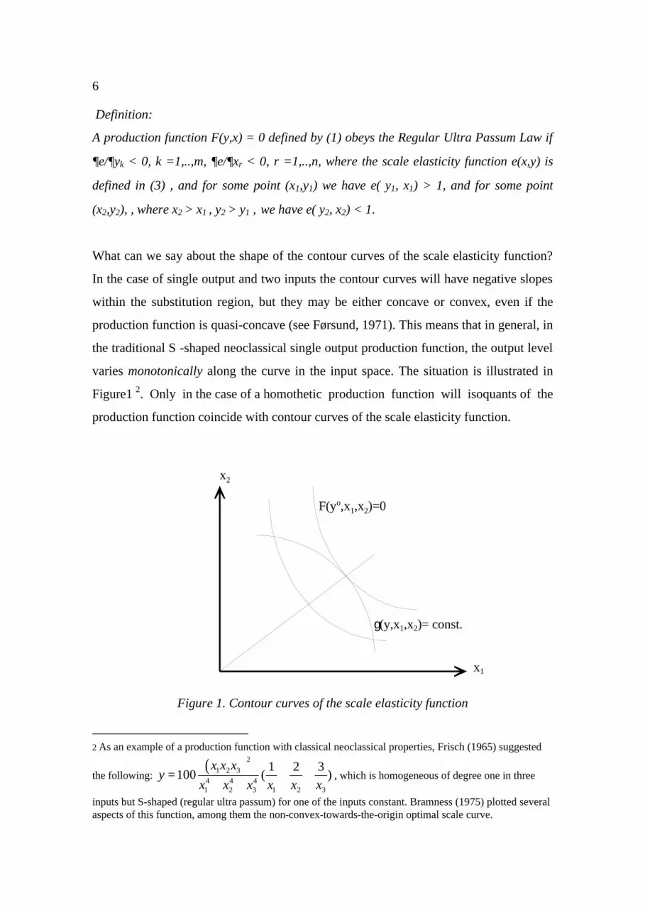
What can we say about the shape of the contour curves of the scale elasticity function?

In the case of single output and two inputs the contour curves will have negative slopes

within the substitution region, but they may be either concave or convex, even if the

production function is quasi-concave (see Førsund, 1971). This means that in general, in

the traditional S -shaped neoclassical single output production function, the output level

varies monotonically along the curve in the input space. The situation is illustrated in

Figure1 2. Only in the case of a homothetic production function will isoquants of the

production function coincide with contour curves of the scale elasticity function.

Figure 1. Contour curves of the scale elasticity function

2 As an example of a production function with classical neoclassical properties, Frisch (1965) suggested

the following: ( )2

1 2 34 4 41 2 3 1 2 3

1 2 3100 ( )

x x xy

x x x x x x= + +

+ +, which is homogeneous of degree one in three

inputs but S-shaped (regular ultra passum) for one of the inputs constant. Bramness (1975) plotted several aspects of this function, among them the non-convex-towards-the-origin optimal scale curve.

x2

x1

g(y,x1,x2)= const.

F(yo,x1,x2)=0

7

The optimal scale curve

It is one contour curve of the scale elasticity function that is of special importance. The

locus of ε(y,x) =1 in the input space was introduced by Frisch (1965) as the techncially

optimal scale curve (TOPS):

{ }0),(,1),(:),( === xyFxyxyTOPS ε (4)

For movements along factor rays the productivities are maximal on the curve in the

single output case (illustrated in Figure 1 for ε(y, x1,x2) =1), or in the general case of

multiple outputs the ratio β/µ is maximised. Notice from Figure 1 that there is no limit

on the variation of the optimal scale value in the general case. So what would be the

recommendation for optimal scale? The point is that this can only be a relevant question

when the factor prices are known. The point of intersection between the expansion path

and the TOPS curve is the text-book long-run equilibrium point for a unit in a

competitive market (disregarding any problems with a finite number of units), assuming

that it is relevant to operate with constant factor prices. Thus a recommondation of

adjusting to optimal scale has a relevant frame of reference.

In the case of a single output transforming the optimal scale curve into the input

coefficient space it becomes the efficiency frontier (EFF):

=== 0),..,,(,1),..,,(:),..,( 111

nnn xxyFxxyyx

yx

EFF ε (5)

This is made up of all points where the input coefficients reach their minimum along

rays from the origin. Since the optimal scale curve is a contour curve we have from the

section above that the shape of the technically optimal scale curve may vary between

production functions. Even if the production function is quasi-concave, the elasticity of

scale function may not have this property, i.e. the optimal scale curve may or may not be

convex towards the origin. But we note that in the neoclassical world the output level in

the single output case varies monotonically along the curve and then also along the

efficiency frontier. In the case of the production function (1) being simultaneous

homothetic (Hanoch, 1970) we have that the optimal scale contour in input space for

fixed outputs coincide with an input isoquant, and for fixed inputs it coincides with an

8

output isoquant (in the terminology of Frisch, 1965). Simultaneous homotheticity in the

case of variable returns to scale implies that the production function is separable; F(y,x)

= f(y)g(x) (Hanoch (1970), p. 425). In the single output case there is then a unique

optimal scale level independent of the factor ratio elaboration.

The M - locus

The concept of the M - locus in the case of multi output was introduced in Baumol et al.

(1982) to designate the set of all output vectors that minimise average ray costs along

their own ray. Thus, in our setting, the M - locus corresponds to the technically optimal

scale extended to the multi output case, i.e. the geometric locus in output space for all

points where the scale elasticity equals one (see Baumol et al. (1982), p. 58):

{ }0),(,1),(: === xyFxyyM ε (6)

The shape of the M - locus is an important diagnostic for determining the number of

firms in an industry and thereby the market structure. The crucial information is the

difference between industry outputs and the output levels at the M - locus. It is

conjectured that the shape may be irregular (pp. 58-59) and that the distance from the

origin in output space may differ substantially between rays. This is the problem with

determining the number of firms in an industry: the number may be dependent on the

output mix. But one main conjecture in the two-dimensional illustration in Baumol et al.

(Figure 3D1, p. 58) is that there is a trade-off between efficient output levels, similar to

a traditional transformation curve in output space. In the case of two outputs and one

input the M-locus must be a falling curve in the output space.

Introducing inefficiency

So far efficient operations have been assumed. We need a production technology where

both feasible efficient and inefficient point can be identified. A production possibility

set S is in general defined by:

{ }):),( yproducecanxxyS = (7)

We then need to distinguish between efficient and inefficient poins as subsets of the

production set S. The connection between the neoclassical production function (1) and

9

the production set formulation (7) is as follows (see Hanoch (1970), and McFadden

(1978), which states conditions for a unique connection) , with standard properties of S:

{ } { }0),(:),():),( ≤≡= xyFxyyproducecanxxyS (8)

The subset of efficient point is then defined by F(y,x) = 0.

It should be born in mind that returns to scale is a local property and applies only to

efficient points, i.e. points satisfying F(y,x) = 0. To associate an inefficient point with a

scale elasticity value is at best ambiguous, because the existence of inefficieny means

that the local increase in output when inputs are increased cannot be separated from the

increase due to a reduction in inefficiency3. Therefore, a very basic observation for the

discussion of scale properties using the DEA model is that inefficient observations must

first be represented by efficient points. Thus the discussion of scale properties for

inefficient units must be conditional on a meaningful and interesting representation.

The DEA model

The efficient subset in the DEA model corresponding to F(y,x) = 0 maintains the

convexity of isoquants, but in the case of variable returns to sale (VRS) the origin is not

assumed to be in the set, and it is convex. The surface is made up of facets, thus we do

not have differentiability at corners or along ridges. Rates of substitution and rates of

transformation are constant on a facet, and changes from facet to facet. Although we

have to take these features into account we can use the basic definition (2) of the scale

elasticity (see e.g. Banker et al. (1984), Førsund, 1996). Specificially, the optimal scale

curve, the efficiency frontier and the M - locus all exist in the DEA model. These

concepts all belong to a VRS frontier function.

It has become a common practice in the field of non-parametric efficiency analysis to

name the linear programme for the calculation of all Farrell (1957) technical efficiency

3 Banker (1984) and Banker et al. (1984) are clear on this point. However, notice that a set is usually defined as having constant returns to scale if all finite points on rays belong to the set, i.e. the set is a cone. The definition of economies of scale in Panzar and Willig (1977) as a property of the production set in general is rather awkward.

10

scores for the DEA model. The efficiency scores for the VRS input- and output oriented

DEA models, E1i and E2i respectively for unit i, are found by solving the following two

linear programmes:

(9)

(10)

The constraints in (9) and (10) represent the definition of the piecewise linear

technology relevant for unit i. This unit may be inefficient in e.g. its use of inputs. The

input vector in (9) is adjusted by the efficiency score, θi, and then compared with the

reference point, ∑ =

J

j njj x1λ , on the frontier. To find the optimal scale units, the simplest

procedure is to use either model (9) or (10) without the constraint that the sum of

weights add up to one, i.e. the CRS envelopment. The optimal scale units are then

identified by having no slacks on the input (or output) constraints and an efficiency

score of 14.

Jj

Nnxx

Mmyy

ts

MinE

j

J

jj

J

jnjjnii

J

jmimjj

ii

,..,1,0

1

,..,1,0

,..,1,0

..

1

1

1

1

=≥

=

=≥−

=≥−

=

∑

∑

∑

=

=

=

λ

λ

λθ

λ

θ

Jj

Nnxx

Mmyy

ts

MaxE

j

J

jj

J

jnjjni

J

jmiimjj

ii

,..,1,0

1

,..,1,0

,..,1,0

..

1

1

1

1

2

=≥

=

=≥−

=≥−

=

∑

∑

∑

=

=

=

λ

λ

λ

φλ

φ

11

The Regular Ultra Passum Law and the DEA model

We want to investigate whether the DEA model fulfills the Regular Ultra Passum Law

or not. One way of doing this is to use the scale elasticity function for a DEA model

based on the approach first introduced in Banker et al. (1984) (see also Førsund (1996),

Førsund and Hjalmarsson, 1996). We then need the dual programmes to the problems

(9) and (10). Let umi and vni be the non-negative shadow prices on the output- and input

constraints respectively in the optimisation problem (9), and uiin the (unrestricted) shaow

price on the convexity constraint. The dual problem is then:

Jjuxvyu

xv

tosubject

uyuMax

ini

N

nnjnj

M

mmjmj

N

nnini

M

m

inimimi

,..,1,0

1

11

1

1

=≤+−

=

+

∑∑

∑

∑

==

=

=

(11)

Using the same symbols for the shadow prices on the constraints in problem (10) and

calling the (unrestricted) shadow price on the convexity contraint for uiout we have the

dual problem:

Jjuxvyu

yu

tosubject

uxvMin

outi

N

nnjnj

M

mmjmj

M

mmjmj

outi

N

nnini

,..,1,0

1

11

1

1

=≤++−

=

+

∑∑

∑

∑

==

=

=

(12)

The values of the shadow prices uiin and ui

out determine the scale property. In the case of

a input-oriented (output- oriented) reference point we have increasing returns when uiin

(-uiout) > 0, constant when ui

in (uiout) = 0 and decreasing returns when ui

in (-uiout ) < 0.

It is shown in Førsund and Hjalmarsson (1996) that the scale elasticity function in (3)

4 We will not go into details about how to deal with multiple solutions.

12

can be written in the following two equivalent ways for the two reference points

corresponding to an inefficient unit, i:

outiiii

i

inii

iiii

uExyE

uEE

xEy

22

1

11

1),1

(

),(

−=

−=

ε

ε (13)

We will assume that the reference points are in the interior of frontier function facets so

we can differentiate the scale elasticity function at the reference point. Differentiating

the first expression in (13) w.r.t. the ouput type m for unit i yields:

MmuE

uuuEyE

u

yxEy

inii

miini

inii

mi

iini

mi

iii ,..,1,)()(

),(2

12

1

1

1 =−

−=−∂∂

−=∂

∂ε (14)

The last expression is obtained using the Envelope Theorem on the Lagrangian function

for the problem (9), yielding mimii uyE =∂∂ 15. We see from (14) that the sign of the

partial derivative of the scale elasticity function w.r.t. an output depends on the sign of

the shadow price uiin. For increasing returns, ui

in > 0, we have a falling value of the

scale elasticity in accordance with the requirement of the Regular Ultra Passum Law,

but for decreasing returns, uiin < 0, we have an increasing value of the scale elasticity in

contradiction of the law.

Differentiating the second expression in (13) w.r.t. the ouput type m for unit i yields:

NnEvuxE

ux

xyE

iniouti

ni

iouti

ni

nimii ,..,1,

),1

(22

22 ==∂∂

−=∂

∂ε (15)

The last expression is again obtained by using the Envelope Theorem on the Lagrangian

function for problem (10) for investigating the impact of a parameter change, yielding

niinii vExE 222 −=∂∂ . Increasing returns to scale, ui

out < 0, yields a decreasing scale

5 We assume that the basis in the LP solution for (9) does not change, so the shadow prices remain unchanged.

13

elasticity in accordance with the Regular Ultra Passum Law, while decreasing returns to

scale, uiout > 0, yields an increasing scale elasticity, violating the law.

An illustration

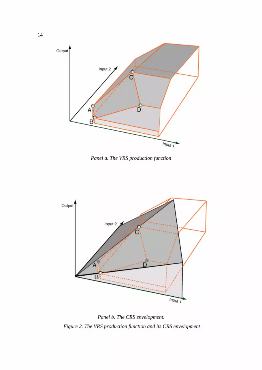
Before reporting the empirical results, a stylised figure (Figure 2) based on only four

units may enhance our understanding of the character of returns to scale in DEA6. All

points are efficient in the case of a variable returns to scale (VRS) envelopment shown

in Panel a. Panel b shows the difference in frontier surfaces between VRS and constant

returns to scale (CRS) envelopment. We see that of the four units two of them, B and C,

are optimal scale units. Unit C has maximal output level, while unit B has the minimal.

The lesson from the stylised figure is that it may be quite normal, even in the case of a

single output, to have both the maximal and minimal output level as the optimal scale.

The central facet has the points A,B,C, D as corners. The technically optimal scale curve

will be a line from B to C in Panel a, with a corresponding variation in the factor ratio.

Notice that it seems easy to calibrate the points B and C such that the optimal scale

curve will be a rising curve in the input plane, in violation of the Regular Ultra Passum

Law. If we cut the surface of the production function in Panel a with a plane, parallel

with the output axis, along a factor ray between the values for points A and B, then the

scale elasticity is infinite at the left-hand side of the intersection point of the plane and

the facet border betwen A and B, and has a value greater than one at the right-hand side

of the intersection point. When the plane intersects the optimal scale curve , a line from

B to C, the scale elasticity obtains the value of one, and on the left-hand side of the

intersection point with the facet border between C and D the scale elasticity obtains a

value less than the value on the left-hand side, but will end up at the left-hand side of the

north- east border of the facet with a higher value than the starting value, although this

will be smaller than the left-hand value on the facet border between C and D. On the

”flat ” facet North-East of point C the value of the scale elasticity will be zero.

6 We are indebted to Dag Fjeld Edvardsen for making the figure.

14

Panel a. The VRS production function

Panel b. The CRS envelopment.

Figure 2. The VRS production function and its CRS envelopment

15

3. Data and model specification

In the empirical application we will select our data from a set of data which have been

utilised in previous work7. The set constitutes a four output - four input model covering

Swedish electric distribution utilities, and was earlier applied in Hjalmarsson and

Veiderpass (1992a) and (1992b), Kumbhakar and Hjalmarsson (1997) and also in Zhang

and Bartels (1998). The data applied in this study cover 163 Swedish electricity retail

distributors in 1987. Only distributors who supply more than 500 low voltage customers

are included. The data are constructed based on information obtained from the

Association of Swedish Electric Utilities (SEF), Statistics Sweden (SCB) and different

retail distributors.

Modelling of electric utilities varies (see Jamasb and Pollitt (2001) for a review of

model specifications). The maximal disaggregation our data allows is to specify four

outputs and four inputs. As regards choice of output measure we consider the total

amount of low and high voltage electricity in MWhs received by the customers (Y1, Y2)

and the number of low and high voltage customers served (Y3, Y4) as the four outputs.

On the input side we use kilometers of low and high voltage power lines (K1, K2) and

total transformer capacity (K3) in kVa as the capital variables. Labour L is measured in

full time equivalent employees. Max, min and mean statistics are shown in Table 1.

However, more aggregate models can also be found in the literature. We will therefore

specify different models that can be used to study the derived economic concepts such

as technically optimal scale curve, the efficiency frontier and the M - locus. We will use

the optimal scale results from three different models. Model 1 is a single-output, two-

input model with total electricity (Y = Y1+Y2) as output and labour and transformer

capacity as inputs. Model 2 is a two-output two-input model with total electricity

(Y1+Y2) and total number of customers

7 In Førsund and Hjalmarsson (1996) we also use a single output, two input data set for Swedish dairies.

16

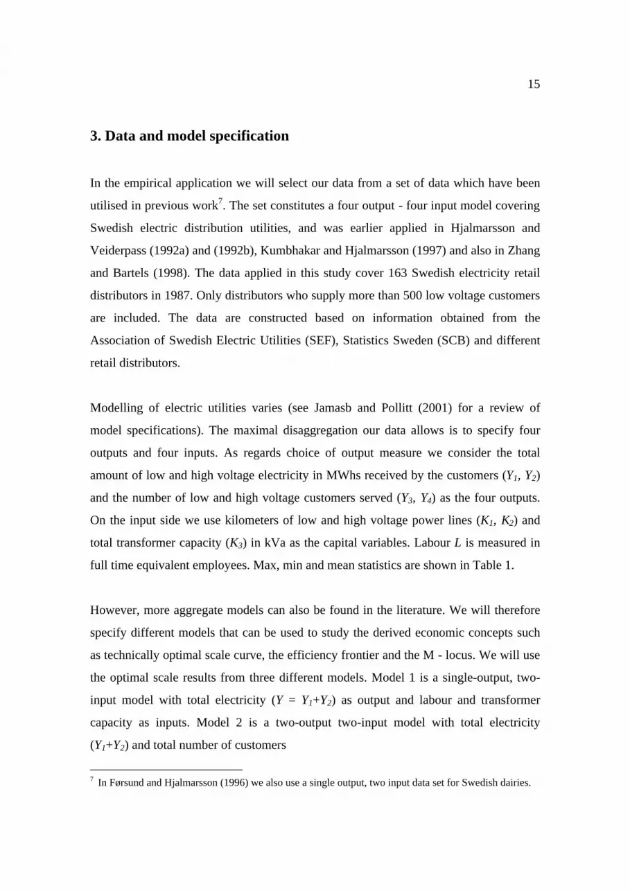
Table 1.List of variables and key statistics

(Y3+Y4) as outputs and labour and transformer capacity as inputs. Model 3 contains all

four outputs and all four inputs; see Table 2.

4. Empirical results

Because of the many outputs and inputs dealt with, between 10 and 53 units out of 163

are on the frontier in the case of variable returns to scale. Among these between 3 and

25 are optimal scale units; see Table 2. We have also added the number of units within

the models. Notice that the largest unit is of optimal scale in all models. In Model 1

about 25% of the units are within the range of optimal scale sizes, in Model 2 about

60% and in Model 3 about 90%.

Table 2. The number of optimal scale and frontier units

*) Both output- and input orientations are run

Y1 MWh low voltage

Y2 MWh high

voltage

Y3 Customers low voltage

Y4 Customers high voltage

L Labour

K1 Lines in Km low voltage

K2 Lines in Km high voltage

K3 Transformers

in kVa

Mean 286057 665979 22841 36 133 1168 989 155434 Stdev 3454887 46644285 225909 641 6493 21159 40783 1801496 Min 9190 0 695 0 2 21 8 4000 Max 4895138 65966223 422793 908 9189 30033 57733 2554000

Model Outputs Inputs Frontier units, VRS

Optimal scale units

Units within the optimal scale range

Total sample

1 Y = Y1 + Y2 L, K3 10 3 39 163

2 Y1+Y2, Y3 + Y4 L, K3 15 4 97,99* 163

3 Y1, Y2, Y3, Y4 L, K1, K2, K3 53 25 146 163

17

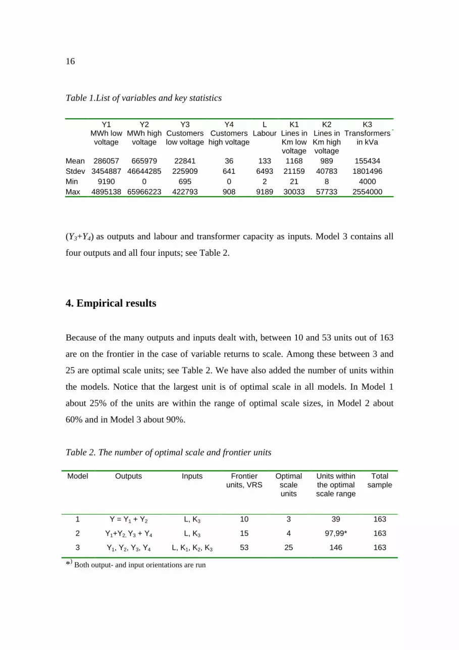
Optimal scale curves

All the optimal scale values in the input space with labour, L, and transformer capacity,

K3, in Model 1 is plotted in Figure 3. This is the technically optimal scale curve

introduced in Frisch (1965). The most striking feature in our DEA case is the positive

slope of the curve. In the case of a classical S-shaped production function, the Regular

Ultra Passum Law introduced in Section 2, the optimal scale curve has a negative slope.

Moreover, when moving along the locus of optimal scale in the input space, the optimal

scale values either increase or decrease monotonically with the factor ratio, or remain

constant in the homothetic case. Although the opposite may occur for other sets of data,

this is also the case in Figure 3, where the smallest unit has a size about 10% of the

second to smallest unit, which in turn has a size about 5% of the largest unit. However,

the slope is in contradiction of the Regular Ultra Passum Law. But as indicated in Figure

2, a positive slope of the curve may well occur.

In the case of DEA, some times small changes in factor ratio “cause” large changes in

optimal scale. This is obvious from Figure 3, where a small change in the factor ratio

causes a large change in optimal scale. Moreover, the largest optimal scale level occurs

at a relatively low capital-labour ratio. A priori, one might expect the opposite, namely

that more capital-intensive technologies coincide with large optimal scale levels.

18

0

500000

1000000

1500000

2000000

2500000

3000000

0 1000 2000 3000 4000 5000 6000 7000 8000 9000 10000

L

K3

Figure 3. The optimal scale curve

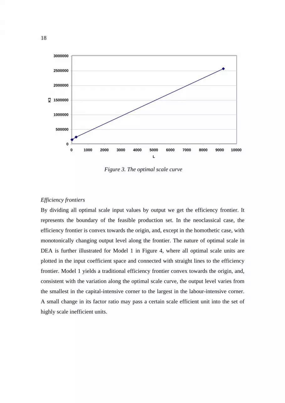
Efficiency frontiers

By dividing all optimal scale input values by output we get the efficiency frontier. It

represents the boundary of the feasible production set. In the neoclassical case, the

efficiency frontier is convex towards the origin, and, except in the homothetic case, with

monotonically changing output level along the frontier. The nature of optimal scale in

DEA is further illustrated for Model 1 in Figure 4, where all optimal scale units are

plotted in the input coefficient space and connected with straight lines to the efficiency

frontier. Model 1 yields a traditional efficiency frontier convex towards the origin, and,

consistent with the variation along the optimal scale curve, the output level varies from

the smallest in the capital-intensive corner to the largest in the labour-intensive corner.

A small change in its factor ratio may pass a certain scale efficient unit into the set of

highly scale inefficient units.

19

0

0.05

0.1

0.15

0.2

0.25

0.3

0.35

0.4

0.45

0 0.00002 0.00004 0.00006 0.00008 0.0001 0.00012 0.00014

L/(Y1+Y2)

K3/

(Y1+

Y2)

Figure 4. The efficiency frontier

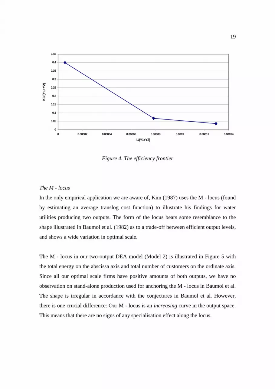
The M - locus

In the only empirical application we are aware of, Kim (1987) uses the M - locus (found

by estimating an average translog cost function) to illustrate his findings for water

utilities producing two outputs. The form of the locus bears some resemblance to the

shape illustrated in Baumol et al. (1982) as to a trade-off between efficient output levels,

and shows a wide variation in optimal scale.

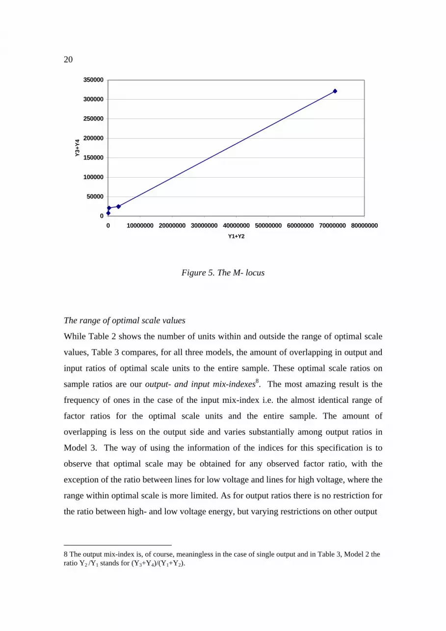
The M - locus in our two-output DEA model (Model 2) is illustrated in Figure 5 with

the total energy on the abscissa axis and total number of customers on the ordinate axis.

Since all our optimal scale firms have positive amounts of both outputs, we have no

observation on stand-alone production used for anchoring the M - locus in Baumol et al.

The shape is irregular in accordance with the conjectures in Baumol et al. However,

there is one crucial difference: Our M - locus is an increasing curve in the output space.

This means that there are no signs of any specialisation effect along the locus.

20

0

50000

100000

150000

200000

250000

300000

350000

0 10000000 20000000 30000000 40000000 50000000 60000000 70000000 80000000

Y1+Y2

Y3+

Y4

Figure 5. The M- locus

The range of optimal scale values

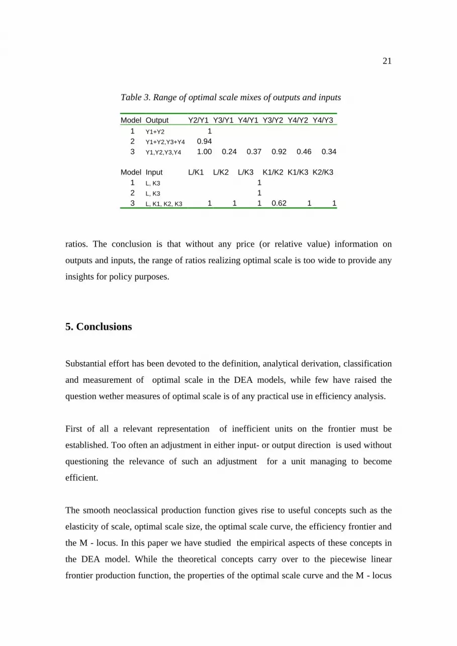
While Table 2 shows the number of units within and outside the range of optimal scale

values, Table 3 compares, for all three models, the amount of overlapping in output and

input ratios of optimal scale units to the entire sample. These optimal scale ratios on

sample ratios are our output- and input mix-indexes8. The most amazing result is the

frequency of ones in the case of the input mix-index i.e. the almost identical range of

factor ratios for the optimal scale units and the entire sample. The amount of

overlapping is less on the output side and varies substantially among output ratios in

Model 3. The way of using the information of the indices for this specification is to

observe that optimal scale may be obtained for any observed factor ratio, with the

exception of the ratio between lines for low voltage and lines for high voltage, where the

range within optimal scale is more limited. As for output ratios there is no restriction for

the ratio between high- and low voltage energy, but varying restrictions on other output

8 The output mix-index is, of course, meaningless in the case of single output and in Table 3, Model 2 the ratio Y2 /Y1 stands for (Y3+Y4)/(Y1+Y2).

21

Table 3. Range of optimal scale mixes of outputs and inputs

ratios. The conclusion is that without any price (or relative value) information on

outputs and inputs, the range of ratios realizing optimal scale is too wide to provide any

insights for policy purposes.

5. Conclusions

Substantial effort has been devoted to the definition, analytical derivation, classification

and measurement of optimal scale in the DEA models, while few have raised the

question wether measures of optimal scale is of any practical use in efficiency analysis.

First of all a relevant representation of inefficient units on the frontier must be

established. Too often an adjustment in either input- or output direction is used without

questioning the relevance of such an adjustment for a unit managing to become

efficient.

The smooth neoclassical production function gives rise to useful concepts such as the

elasticity of scale, optimal scale size, the optimal scale curve, the efficiency frontier and

the M - locus. In this paper we have studied the empirical aspects of these concepts in

the DEA model. While the theoretical concepts carry over to the piecewise linear

frontier production function, the properties of the optimal scale curve and the M - locus

Model Output Y2/Y1 Y3/Y1 Y4/Y1 Y3/Y2 Y4/Y2 Y4/Y3 1 Y1+Y2 1 2 Y1+Y2,Y3+Y4 0.94 3 Y1,Y2,Y3,Y4 1.00 0.24 0.37 0.92 0.46 0.34

Model Input L/K1 L/K2 L/K3 K1/K2 K1/K3 K2/K3

1 L, K3 1 2 L, K3 1 3 L, K1, K2, K3 1 1 1 0.62 1 1

22

do not. Neither is the Regular Ultra Passum Law obeyed. The efficiency frontier

behaves as in neo-classical production theory because it is based on the basic convexity

of the producion set.

The empirical application illustrates some problems with these concepts in applied DEA

analyses. The range of optimal scale levels may be extremely wide, as may be the range

of factor ratios for the set of optimal scale units. Inclusion or exclusion of a few DMUs

may have a large effect on the set of optimal scale units and their size. In a technical

sense the scale properties revealed by a DEA study is correct, provided the outputs or

the inputs are changed in a strictly proportional fashion. But this is not very comforting

for policy recommendations when optimal scale changes dramatically from one output-

or input ray to the other. A fundamental problem with DEA applications arise in the

case when there are no output- or input prices, which often is the case, at least for

outputs, for public sector applications. Without expansions paths in input- and output

space as reference change of input-and output mix may be as relevant as proportional

scaling up or down along observed proportions.

What about scale efficiency? Scale efficiency is a relative concept tied to optimal scale.

The scale efficiency of a certain unit depends on its benchmark or yardstick unit - not on

its absolute size. This benchmark may vary substantially for small changes in input and

output mix of a specific unit. Therefore, scale efficiency is as ambiguous empirically as

a basis for recommendations for change as optimal scale.

What about input- and output oriented Farrell technical efficiency measures, the raison

d’etre of DEA studies? The situation is different for these measures, because the key

question here is the distance to the frontier, according to some common rule of

measuring distance. One is not pursuing a recommendation for a specific change, just to

point out a potential for an improvement.

A general problem with estimating production functions is whether the specification of

the production relations is sufficiently close to what we want to model. A feature often

23

regarded as a strenght of the non-parametric DEA model is that it reflects just the

observations and no preconceived functional form. However, the DEA model may be

too data dependent; the model as it is usually specified may lack enough structure to

generate credible information about optimal scale levels. We should recall that the scale

elasticity and optimal scale level are derived along rays.The general nature of the

requirements for properties across rays, i.e. requirements about shapes of isoquants and

transformation curves may not be enough to sufficiently mirror the real life engineering

restrictions on substitution and transformation not captured by the DEA model

specification9.

Our recommendation to the dilemmas for policy conclusions based on DEA models as

to optimal scale is to show the empirical scope for output- and input mixes of optimal

scale. In the case of wide scopes there is no way around using price data for outputs and

inputs to establish a frame of reference for scale adjustments. The prices may be

observed or of a shadow price nature, especially for outputs.

References

Banker, R. D. (1984): “Estimating most productive scale size using data envelopment

analysis”, European Journal of Operational Research 17, 35-44.

Banker, R. D., Charnes, A., and W. W. Cooper (1984): "Some models for estimating

technical and scale inefficiencies", Management Science 39, 1261-1264.

Baumol, W. J., J. C. Panzar, and R. D. Willig (1982): Contestable markets and the

theory of industry structure, New York: Harcourt Brace Jovanovich.

9 Note that the neoclassical formulation F(y,x) = 0 is a very general formulation too, may be too general, cf. the considerably more elaborate formulation in Frisch (1965). See also Førsund (1999) for a review of Frisch's production theory and engineering production functions.

24

Bramness,G. (1975): “Notat om et analytisk eksempel pa en regular ultra-passum-lov”

(An example of an analytical regular ultra passum production function.), Memorandum,

Department of Economics, University of Oslo.

Farrell, M. J. (1957): “The measurement of productive efficiency”, Journal of the Royal

Statistical Society, Series A (General) 120 (III), 253-281(290).

Frisch, R. (1965): Theory of production, Dordrecht: D. Reidel.

Førsund, F.R. (1971): "A note on the Technically Optimal Scale in inhomogeneous

production functions", Swedish Journal of Economics 73, 225-240.

Førsund, F.R. (1996): “On the calculation of the scale elasticity in DEA models”,

Journal of Productivity Analysis 7, 283-302.

Førsund, F.R. (1999): “On the contribution of Ragnar Frisch to production theory",

Rivista Internazionale di Scienze Economiche e Commerciali (International Review of

Economics and Business) XLVI, 1-34.

Førsund, F.R., and L. Hjalmarsson (1996): “Measuring returns to scale of piecewise

linear multiple output technologies: Theory and empirical evidence”, Memorandum No

223, Department of Economics, School of Economics and Commercial Law, Göteborg

University.

Hanoch, G. (1970): "Homotheticity in joint production", Journal of Economic Theory 2,

423-426.

Hjalmarsson, L. and A. Veiderpass (1992a): “Efficiency and ownership in Swedish

electricity retail distribution”, Journal of Productivity Analysis 3, 7-23.

25

Hjalmarsson, L. and A. Veiderpass (1992b): “Productivity in Swedish electricity retail

distribution”, Scandinavian Journal of Economics 94, Supplement, 193-205.

Jamasb, T. and M. Pollitt (2001): “Benchmarking and regulation: international

electricity experience”, Utilities Policy 9(3), 107-130.

Kim, H. Y. (1987): “Economies of scale in multi-product firms: an empirical analysis”,

Economica 54, 185-206.

McFadden, D. (1978): "Cost, revenue and profit functions", in M. Fuss and D.

McFadden (eds.): Production economics: A dual approach to theory and applications,

Vol. 1, Chapter 1, 3-109, Amsterdam: North Holland Publishing Company.

Kumbhakar, S.C., and L. Hjalmarsson (1997): “Relative performance of public and

private ownership under yardstick regulation”, European Economic Review 42, 97-122.

Kumbhakar, S.C. and Lovell, C.A.K. (2000): Stochastic Frontier Analysis, Cambridge:

Cambridge University Press.

Panzar, J. C. and R. D. Willig (1977): "Economies of scale in multi-output production",

Quarterly Journal of Economics XLI, 481-493.

Seiford, L. M. (1996): “Data Envelopment Analysis: The Evolution of the State of the

Art (1978-1995)”, Journal of Productivity Analysis 7 (2/3), 99-137.

Starrett, D. A. (1977): "Measuring returns to scale in the aggregate, and the scale effect

of public goods", Econometrica 45, 1439-1455.

26

Zhang, Y. and R. Bartels (1998): “The effect of sample size on the mean efficiency in

DEA with an application to electricity distribution in Australia, Sweden and New

Zealand”, Journal of Productivity Analysis 9, 187-204.