Embed Size (px)
Citation preview
Appendix 5.2 – Details on Hydrodynamic and Water Quality Modelling P. i
APPENDIX 5.2
DETAILS ON HYDRODYNAMIC AND WATER QUALITY MODELLING
Table of Contents
1.1 General Model Description ................................................................................... 1
1.2 Model Selection and Setup .................................................................................. 1
1.3 Model Verification and Validation ......................................................................... 8
List of Figures Figure 5A- 1 Existing grid of the Update Model in the vicinity of Tai O STW ........................ 2
Figure 5A- 2 Local Fine Grid Model in the vicinity of Tai O STW .......................................... 3
Figure 5A- 3 Local Fine Grid Model of Tai O STW ................................................................ 3
Figure 5A- 4 Linkage of the Update Model and Local Fine Grid Model ................................. 4
List of Tables Table 5A- 1 Key Modeling Parameters .......................................................................... 7
Appendix 5.2 – Details on Hydrodynamic and Water Quality Modelling P. 1
1.1 General Model Description
1.1.1 A computer modelling approach was adopted to assess the potential impact on
marine water quality associated with the Project. The Delft3D suite of models,
namely Delft3D-FLOW, Delft3D-WAQ and Delft3D-SED, developed by Delft
Hydraulics, was used as the platform for hydrodynamic, water quality and sediment
plume modelling, respectively. Delft3D is a state-of-the-art computer program that
simulates three-dimensional flow and water quality processes and is capable of
handling the interactions between different hydrodynamic and water quality
processes.
1.1.2 Delft3D-FLOW is a 3-dimensional hydrodynamic simulation module with applications
for coastal, river and estuarine areas. The model calculates non-steady flow and
transport phenomena that result from tidal and meteorological forcing on a curvilinear,
boundary fitted grid. Delft3D-WAQ is a water quality module for numerical simulation
of various physical, biological and chemical processes in three dimensions. It solves
the advection diffusion-reaction equation for a predefined computational grid and for
a wide range of model substances.
1.1.3 A Local Fine Grid Model, which covers the local areas of the proposed project was
set up using the Delft3D suite of models for hydrodynamic and water quality
simulations. The grid sizes of the Local Fine Grid Model were around 30m near the
proposed Tai O STW, which is less than 75m to meet the modelling requirements
specified in the study brief.
1.1.4 The effects on the hydrodynamic regime were determined by examining the changes
in speeds and directions of flow currents, and water levels at selected monitoring
points and cross-sections. Predicted water quality results were compared with
existing regional Update Model for a number of parameters including salinity,
biochemical oxygen demand, ammonia nitrogen, nitrate, dissolved oxygen and
chlorophyll-a, etc.
1.2 Model Selection and Setup
1.2.1 The existing regional model Update Model, which is a fully calibrated and verified
model developed under “Update on Cumulative Water Quality and Hydrological
Effect of Coastal Developments and Upgrading of Assessment Tool Study (1998)” by
EPD based on the Delft3D suite of models, was used to simulate effects on
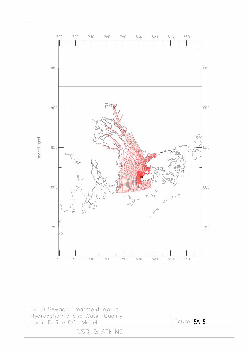
hydrodynamics and water quality. The existing grid of the Update Model in the
vicinity of the Tai O STW is shown in Figure 5A-1. The grid size of the existing
Update Model near the project site is in the order of about 300 m. It is, therefore,
necessary to refine the model mesh to provide improved resolution (less than 75m)
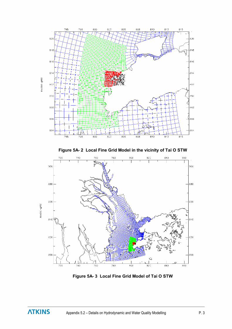
in key areas of interest. A proposed Local Fine Grid Model was used for this EIA for
the vicinity of project area is shown in Figure 5A-2 and Figure 5A-3.
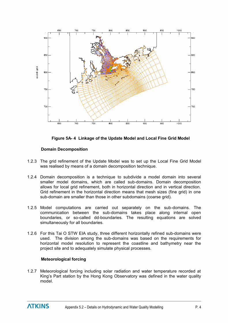
1.2.2 The Local Fine Grid Model was linked to the regional Update Model, which is shown
in Figure 5A-4. Open boundary conditions of the Local Fine Grid Model were
transferred from the Update Model. That is, modelling was first carried out using the
regional Update Model, and the output from the Update Model at the interface with
the Local Fine Grid Model were used as the boundary conditions for input to the
Local Fine Grid Model for both hydrodynamic and water quality simulations. The

Appendix 5.2 – Details on Hydrodynamic and Water Quality Modelling P. 2
cumulative effects from the Pearl River estuaries and pollution loadings were
accounted for in the Update Model, which covers the whole of the Hong Kong waters
and the Pearl River estuaries.
Figure 5A- 1 Existing grid of the Update Model in the vicinity of Tai O STW
Appendix 5.2 – Details on Hydrodynamic and Water Quality Modelling P. 3
Figure 5A- 2 Local Fine Grid Model in the vicinity of Tai O STW
Figure 5A- 3 Local Fine Grid Model of Tai O STW
Appendix 5.2 – Details on Hydrodynamic and Water Quality Modelling P. 4
Figure 5A- 4 Linkage of the Update Model and Local Fine Grid Model
Domain Decomposition
1.2.3 The grid refinement of the Update Model was to set up the Local Fine Grid Model
was realised by means of a domain decomposition technique.
1.2.4 Domain decomposition is a technique to subdivide a model domain into several
smaller model domains, which are called sub-domains. Domain decomposition
allows for local grid refinement, both in horizontal direction and in vertical direction.
Grid refinement in the horizontal direction means that mesh sizes (fine grid) in one
sub-domain are smaller than those in other subdomains (coarse grid).
1.2.5 Model computations are carried out separately on the sub-domains. The
communication between the sub-domains takes place along internal open
boundaries, or so-called dd-boundaries. The resulting equations are solved
simultaneously for all boundaries.
1.2.6 For this Tai O STW EIA study, three different horizontally refined sub-domains were
used. The division among the sub-domains was based on the requirements for
horizontal model resolution to represent the coastline and bathymetry near the
project site and to adequately simulate physical processes.
Meteorological forcing
1.2.7 Meteorological forcing including solar radiation and water temperature recorded at
King’s Part station by the Hong Kong Observatory was defined in the water quality
model.
Appendix 5.2 – Details on Hydrodynamic and Water Quality Modelling P. 5
Vertical Layers of Hydrodynamic Model
1.2.8 The vertical water column was divided into ten layers for hydrodynamic simulation.
The thickness of each water layer in the vertical direction was 10% of the total water
depth from surface to bottom.
Boundary and Initial Conditions
1.2.9 The Local Fine Grid Model was linked to the Regional Model “Update Model”, which
is a fully calibrated and verified model developed under “Update on Cumulative
Water Quality and Hydrological Effect of Coastal Developments and Upgrading of
Assessment Tool Study (1998)” by EPD.
1.2.10 Open boundary conditions of the Local Fine Grid Model were defined by the Update
model. That is, modelling was first carried out using the Update Model, and the
output from the regional Update Model at the interface with the Local Fine Grid
Model were used as the boundary condition for input to the Local Fine Grid Model for
hydrodynamic and water quality simulation. The cumulative effects from the Pearl
River estuaries are accounted for in the Update Model, which covers the entire Hong
Kong waters and the Pearl River estuaries.
Initial and Boundary Conditions
1.2.11 The Local Fine Grid Model was linked to the Update Model. Hydrodynamic
computations were first carried out using the Update Model. The Update Model
provides open boundary conditions to the Local Fine Grid Model through the nesting
process.
1.2.12 The initial conditions for the Local Fine Grid Model were selected to be the same as
those of the Update Model. This was done by using a utility program to map the
information contained in the restart file of the Update Model to the restart file of the
Local Fine Grid Model.
Flow Aggregation for Water Quality Modeling
1.2.13 The grid for water quality simulation was based on the hydrodynamic grid model. To
reduce computation time and computer storage, flow aggregation in the vertical
direction of the grid were performed to reduce the total number of computation cells
for water quality simulation. The thickness distribution of the layers was 10%, 20%,
20%, 30% and 20% of the total water depth from surface to bottom to optimise the
computational time and data storage.
1.2.14 In the horizontal directions, no flow aggregation was planned to be performed to
provide sufficient resolution of modelled results for assessment of impact to Water
Sensitive Receivers in the local areas of the Project.
Simulation Periods and Time Step
1.2.15 For each assessment scenario, the simulation period of the hydrodynamic model
covered two 15-day full spring-neap cycles (excluding the spin-up period) for dry and
Appendix 5.2 – Details on Hydrodynamic and Water Quality Modelling P. 6
wet seasons, respectively.
1.2.16 Water quality simulation also covered two 15-day full spring-neap cycles (excluding
the spin-up period) for dry and wet seasons respectively. A sufficient spin-up period
was provided to ensure that initial condition effects can be neglected.
1.2.17 The time steps in the hydrodynamic and water quality model were tentatively set
equal to 0.5 minute and 0.5 hour, respectively.
Wind
1.2.18 To be identical to the Update Model, a north-eastern wind with a belonging wind
speed of 5 m/s was used for the dry season computations. The wet season
computations applied a south western wind of 5 m/s.
Hydrodynamic Forcing
1.2.19 Hydrodynamic simulations were carried out with the Local Fine Grid Model for a
spring neap cycle for both the wet season and the dry season. The results were
written to a so-called "communication file" in the Delft3D model with a time interval of
1 hour, that is, the hydrodynamic modelling results were saved to a result file every
one hour. Given that the time step for model simulation was tentatively 0.5 minute,
this means that hydrodynamic modelling results were saved to a result file for later
use for water quality simulation once every 120 steps of model simulation. The
intermediate results during the spin-up period of the hydrodynamic model were
omitted in this process, creating the simulating results for two spring-neap tidal
cycles for dry and wet seasons, respectively.
1.2.20 From the communication file, the hydrodynamic forcing data for the water quality
model were derived, by using the coupling module of Delft3D.
Meteorological Forcing
1.2.21 Meteorological forcing was defined in the water quality model. Seasonal variations in
Pearl River discharges, solar radiation and wind velocity were incorporated into the
water quality simulation.
Key Modeling Parameters
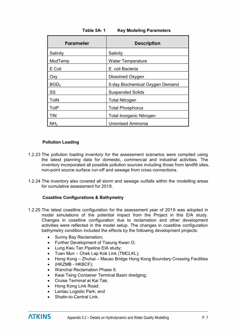
1.2.22 The key water quality parameters to be included in water quality impact assessment
are shown in Table 5A- 1.
Appendix 5.2 – Details on Hydrodynamic and Water Quality Modelling P. 7
Table 5A- 1 Key Modeling Parameters
Parameter Description
Salinity Salinity
ModTemp Water Temperature
E Coli E. coli Bacteria
Oxy Dissolved Oxygen
BOD5 5-day Biochemical Oxygen Demand
SS Suspended Solids
TotN Total Nitrogen
TotP Total Phosphorus
TIN Total Inorganic Nitrogen
NH3 Unionised Ammonia
Pollution Loading
1.2.23 The pollution loading inventory for the assessment scenarios were compiled using
the latest planning data for domestic, commercial and industrial activities. The
inventory incorporated all possible pollution sources including those from landfill sites,
non-point source surface run-off and sewage from cross connections.
1.2.24 The inventory also covered all storm and sewage outfalls within the modelling areas
for cumulative assessment for 2019.
Coastline Configurations & Bathymetry
1.2.25 The latest coastline configuration for the assessment year of 2019 was adopted in
model simulations of the potential impact from the Project in this EIA study.
Changes in coastline configuration due to reclamation and other development
activities were reflected in the model setup. The changes in coastline configuration
bathymetry condition included the effects by the following development projects:
Sunny Bay Reclamation;
Further Development of Tseung Kwan O;
Lung Kwu Tan Pipeline EIA study;
Tuen Mun – Chek Lap Kok Link (TMCLKL);
Hong Kong – Zhuhai – Macao Bridge Hong Kong Boundary Crossing Facilities
(HKZMB - HKBCF);
Wanchai Reclamation Phase II;
Kwai Tsing Container Terminal Basin dredging;
Cruise Terminal at Kai Tak;
Hong Kong Link Road;
Lantau Logistic Park; and
Shatin-to-Central Link.
Appendix 5.2 – Details on Hydrodynamic and Water Quality Modelling P. 8
1.3 Model Verification and Validation
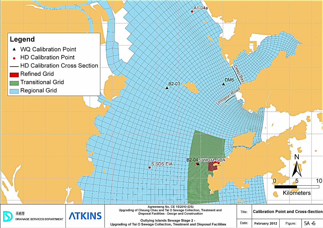
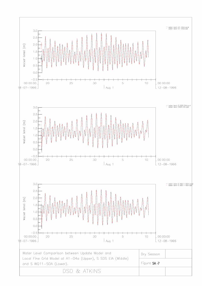
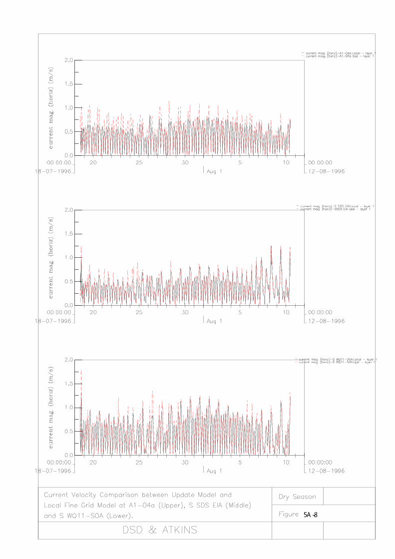
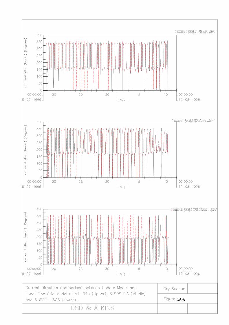
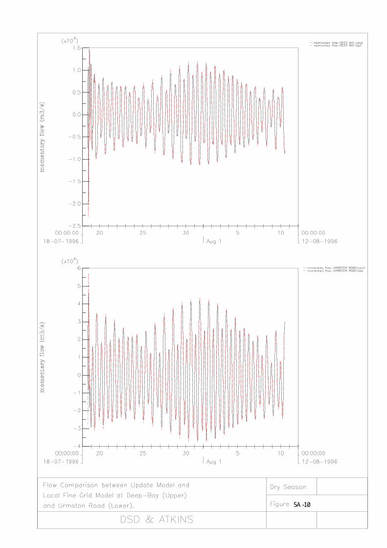
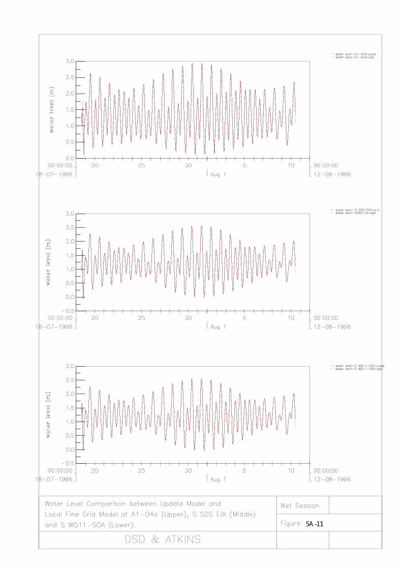
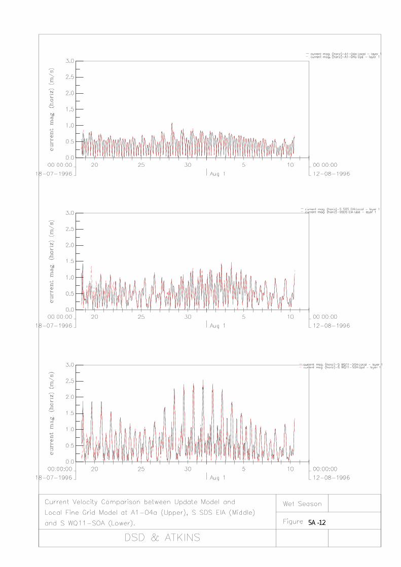
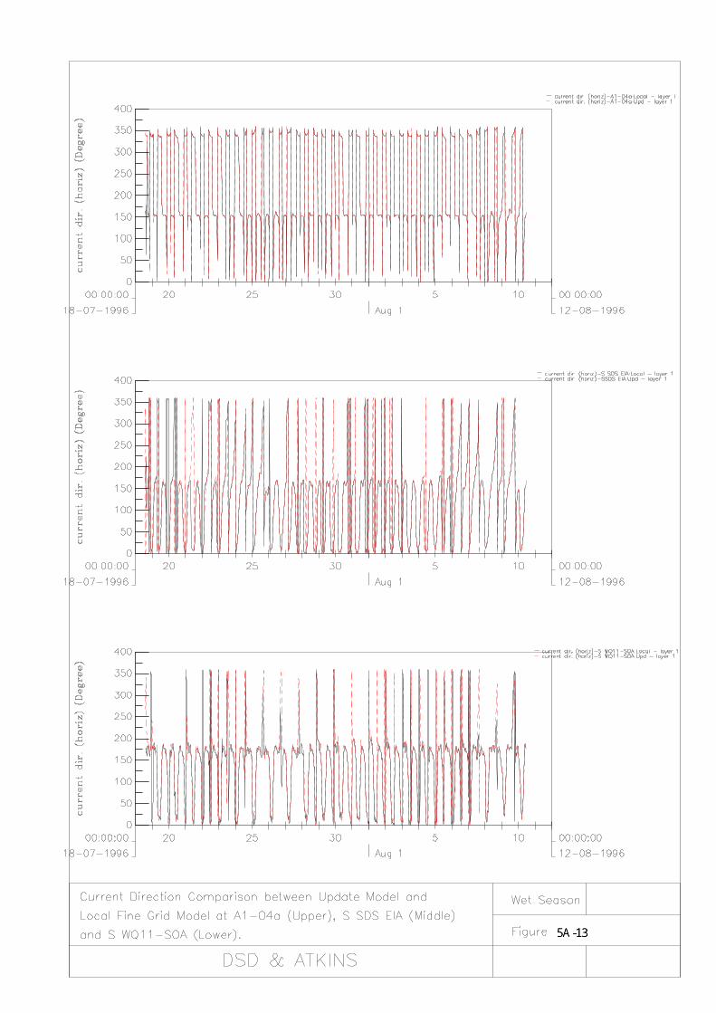
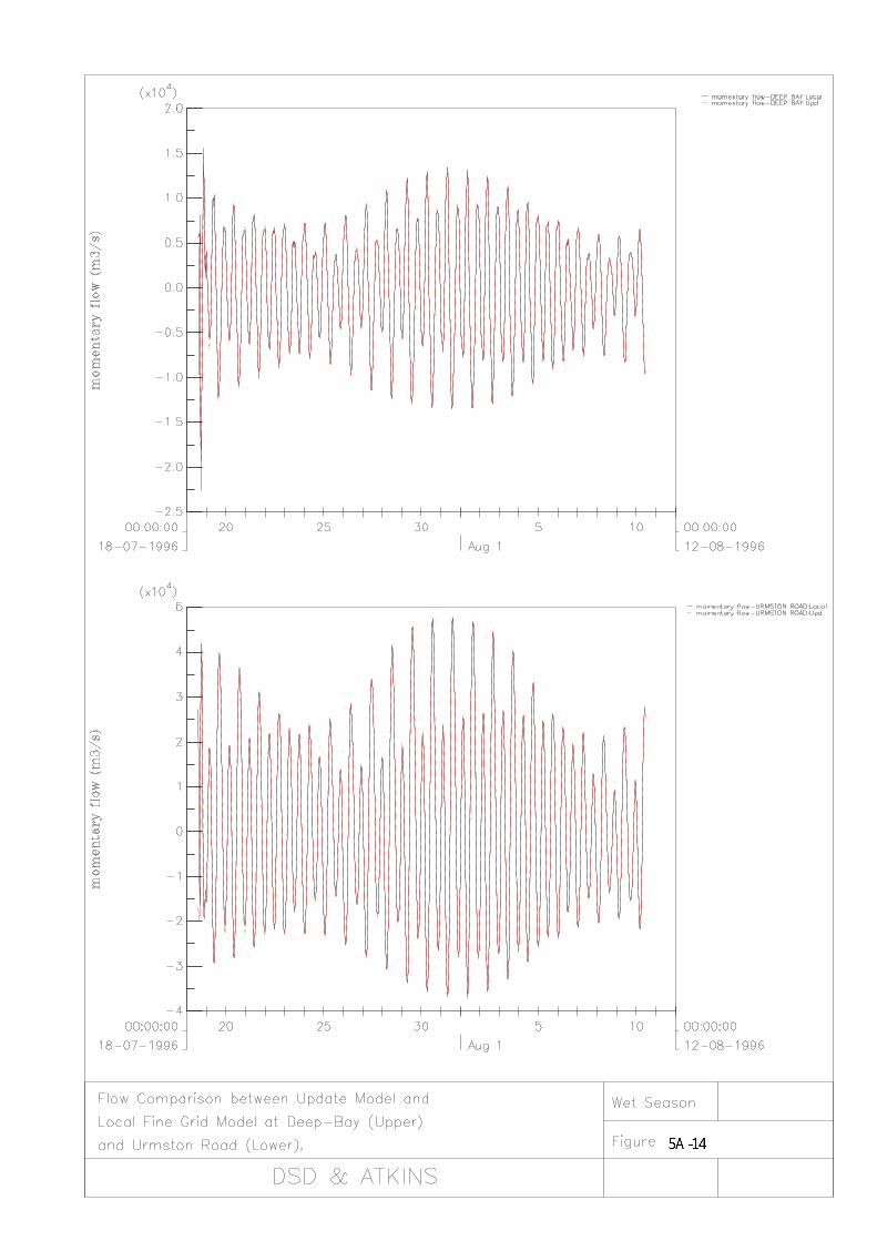
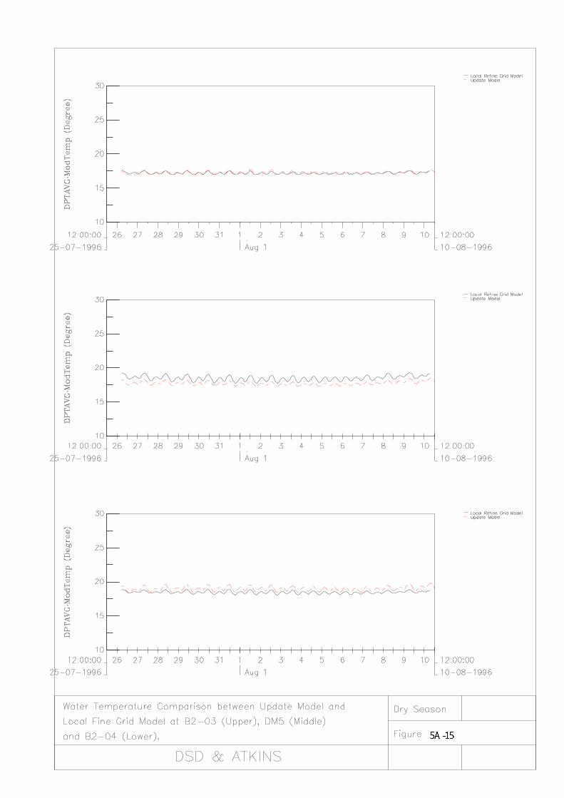
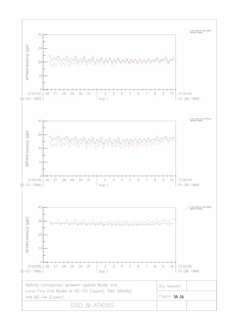
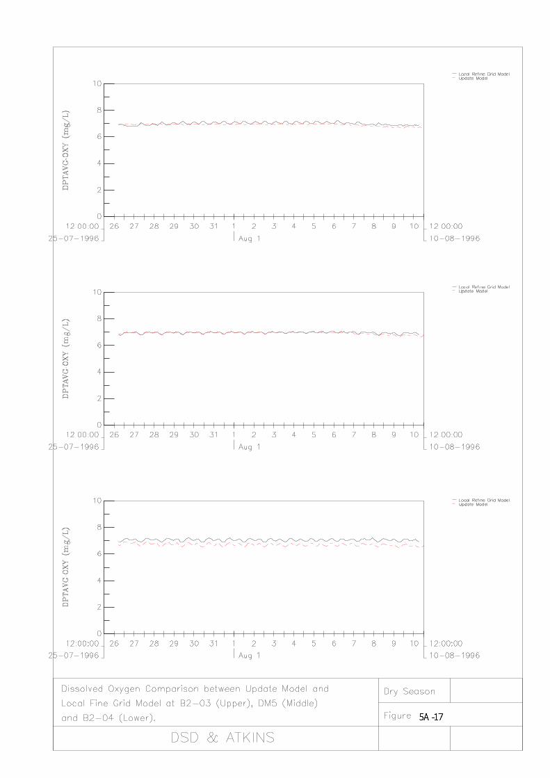
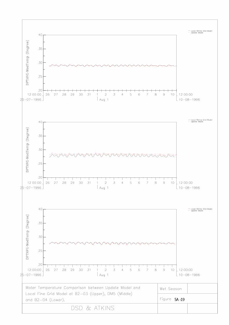
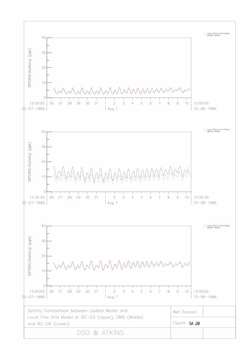
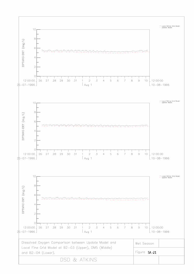
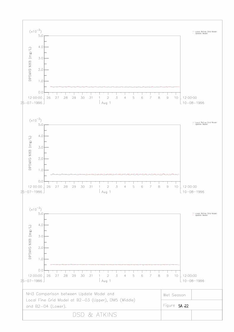
1.3.1 Hydrodynamic and water quality results predicted with the Local Fine Grid Model for
the Tai O STW were compared to those obtained from the Update Model to validate
and calibrate the Local Fine Grid Model. The calibration figures are shown in Figure 5A-5 to Figure 5A-22. The calibration shows that the results from the Local Fine
Grid Model and the Update Model matched well, which indicate that the accuracy of
Local Fine Grid Model can be guaranteed.
1.3.2 Having been calibrated, the Local Fine Grid Model was then used to simulate and
predict the impact on receiving marine waters and water sensitive receivers under
different assessment scenarios.