Age, Experience, and Schooling: Decomposing Earnings Inequality in the United States and Brazil

Age, Experience, Inequality in the

and Schooling: Decomposing Earnings United States and Brazil *

David Lam, University of Michigan and Deborah Levison, Yale University

This article analyzes age and experience profiles of earnings inequality for U.S. and Brazilian males. Decomposition of the inequality profiles using a standard human capital earnings equation clarifies the determinants of cross-sectional inequality profiles and demonstrates a number of important differences in the shape of the two countries’ profiles and in their underlying components. Most dramatic are Brazil’s higher returns to schooling and higher variance in years of schooling, both factors contributing to the significantly higher level of income inequality in Brazil. Changes in the distribution of schooling across cohorts are shown to play a central role in explaining cross-sectional inequality profiles within each country and differences in earnings inequality in the United States and Brazil.

Introduction

Profiles of earnings inequality by age and experience play an important role in explanations of income distributions by labor economists, development economists, and demographers. Age profiles of inequality are important because they determine the relationship between the age composition of the population and the overall distribution of income, an important consideration in intertemporal and cross-national inequality comparisons. ’ Experience profiles of inequality have received attention because of their relationship to human capital models of income distribution. Mincer (1974) derives predictions about the relationship between experience and earnings inequality from a human capital model of investment in schooling and on-the-job training. His notion of an “overtaking point” plays a central role in these predictions and is used by Mincer to quantify the power of the human capital model in explaining earnings inequality.

Experience and Earnings Inequality in a Cohort

In analyzing age and experience profiles of earnings inequality, it is useful to keep in mind Mincer’s predictions about the relationship between earnings inequality and job market experience. Mincer’s basic points can be seen by considering a simple earnings equation for individual i at j years of experience:

Sociological Inquiry, Vol. 62, No. 2, Spring 1992 @1992 by the University of Texas Press, P.O. Box 7819, Austin, TX 78713

EARNINGS INEQUALITY IN THE U.S. AND BRAZIL 221

lnYij = ai + rSi + j o ) + uij (1) where Yij is person 2s earnings in period j , ai = In EiO is the log of earnings person i would have earned with no schooling and no post-schooling human ~ a p i t a l , ~ r is the rate of return to schooling, Si is the number of years of schooling of person i, J(j) is the net return to person 2s post-schooling investments in human capital after j years of experience, and ui is an error term assumed to be uncorrelated with the other determinants of observed earnings.

If we assume that Y is constant across individuals, then for the group of workers with experience j the variance of log earnings implied by (1) is:

v(lnY) = &(a) + y 2 & ( S ) + K(j) + F ( u ) + 2rCi(a,S) + 2rCj(S,j) + 2Cj(a;f) (2)

where F ( x ) and Cj(x,y) represent the variance of x and the covariance of x and y among workers with j years of experience. In the most general case, the variances and covariances in (2) have few restrictions on their signs, magni- tudes, or relationship to years of experience. By putting more structure on the model, however, Mincer was able to make specific predictions about the relationship between the variance in log earnings and experience.

One set of restrictions will hold whenever the same “experience cohort” (that is, a group of workers who began working in the same year, though not all at the same age) is observed over time. If we follow an experience cohort over years of experience, then initial earnings capacity and years of schooling of all individuals in the cohort are determined at the time the cohort enters the labor force. It follows that K(a), K(S), and C’(a) S) will be constant across j , affecting the level but not the shape of the inequality-experience profile. If vJ(u), the pureiy stochastic component of each period’s earnings, is also constant for allj, then the shape of the relationship between the overall variance of log earnings K(ln Y) and experience will be determined by QCf), Cj(a,f), and Cj(S,f).

The second set of restrictions to simplify (2) involves individual investments in post-schooling human capital. Individuals who make post-schooling investments in human capital trade off current earnings for on-the-job training, so that net returns to post-schooling investmentsJ0;) are initially negative during the years in which foregone earnings outweigh the accumulated returns. Eventually accumulated returns exactly equal foregone earnings, after which the returns to post-schooling investments are positive. Mincer called the point at which net returns to human capital switch from negative to positive the “overtaking point.” We denote the overtaking point by j , with fiG) < 0 for j <j, JQ) = 0 and f&) > 0 forj > j . I f j were equal for individuals in all schooling group^,^ then at year of experiencej, earnings would be equal for all workers with the same schooling, independent of their post-schooling investments in human capital. It follows that not only will Kcf) = 0, but also

222 DAVID LAM AND DEBORAH LEVISON

Ci(cuj) = CdS, f) = 0. The variance in log earnings at the “overtaking point” is purged of any influence from post-schooling investments in human capital.’

A third restriction reduces (2) to the simplest and perhaps best known case. Assume that post-schooling investments in human capital are uncorrelated with the level of schooling S and with initial earnings capacity a, imply- ing that Cj(S,j) = Cj(a,fl = 0 for allj. Since v(a), F(S), and Cj(a,S) do not depend on j in an experience cohort, and assuming that V(u) and 7 are constant, (2) is reduced to

wherej subscripts have been dropped for terms assumed to be independent of experience. Under all of these assumptions, the variance in log earnings changes with years of experience for an experience cohort only because of the change in the variance in net returns to post-schooling investments in human capital 50 . Since Ffl reaches a minimum at j , V (In Y ) will also reach a minimum at j , reflecting only the inequality due to the returns to schooling.6

Ffln Y ) = v(a) + 2rC(a,S) + rZV(S) + v(u) + Ffl (3)

Age, Experience, and Earnings in Cross Sections

Although the predictions implied by (2) and its simplified version (3) apply to experience cohorts, empirical applications have typically looked at a cross section of workers of different experience levels, rather than at cohorts (Mincer 1974, 97-1 14; Psacharopoulos 1977; Brown 1980; Psacharopoulos and Layard 1979. Cohort data are analyzed by Hause 1980). Cross-sectional profiles of inequality by age have often been discussed as if they should behave similarly to the experience profiles, a tendency reinforced by the apparent consistency between the two in U.S. data.’ Data limitations, particularly in developing countries, often make the use of cross-sectional data and the analysis of age profiles rather than experience profiles unavoidable. Furthermore, there is a direct interest in analyzing the relationship between inequality and age as well as inequality and experience. Age structure is an important characteristic of any population and, unlike the experience distribution, is independent of economic behavior in the short run. The relationship between age structure and inequality has received considerable attention by development economists and economic demographers, motivated in part by interest in whether the generally higher levels of inequality in developing countries could be directly related to their much younger age structures. It is instructive, then, to consider whether the relationship between inequality and experience in cohorts implied by (3) has implications for the relationship between inequality and experience observed in cross sections or for the relationship between inequality and age in either cohorts or cross sections. While several


important points on this issue have been made by Mincer (1974) and Brown (1980), some additional complexities are worth noting.

There are two issues to consider. First, how do inequality profiles for a cohort relate to inequality profiles in a cross section? Second, how do inequality profiles by years of experience compare to inequality profiles by years of age? A useful framework for analyzing these issues considers the case of discrete schooling groups (which could refer to single years of schooling or to formal schooling levels such as elementary, junior high, and so on). The total variance of log earnings for workers of any given year of age or experience can then be decomposed into within-group and between-group variance. The variance of log earnings for workers with experience j, for example, can be decomposed as

where wij is the proportion of workers with experiencej in schooling group i, yi, is the mean of log earnings for workers with experience j and schooling i, yi is the mean of log earnings for workers with experience j , and u i j ( j ) is the variance of log earnings for workers with experience j and schooling i. The first sum in (4) is the between-group component of total variance, and the second sum is the within-group component. In the framework of earnings equation (l), between-group variance reduces to r2 V(S), with all other components of total variance in (3) included in within-group variance.

The weights w,. in (4) reflect the distribution of years of schooling among workers with the same years of age or experience. Much of the confusion in the analysis of age and experience profiles of inequality arises because of these weights, with schooling groups being weighted differently in the cross section than in the cohort. These differences can be systematically summarized as follows.

Following Mincer, suppose that for every ith schooling group in a cohort, within-group variance uij(j) is determined by post-schooling investments in human capital SO that uijCy) is U-shaped as a function of experience j . From (4) we see, first, that if the population weights wij are constant over the life of an experience cohort, then the within-group variance for the cohort will also be U-shaped, since it is a weighted average of the U-shaped u i j ( j ) schedules with the population weights constant across j . Since by assumption all schooling is completed at the time labor market experience begins, the weights are constant for an experience cohort.’

Second, for an age cohort (that is, a cohort born in the same year followed over their working lives), the schooling distribution (and thus the weights wij) will be constant beginning at the age at which all workers have entered the labor force, abstracting once again from mortality and the acquisition of formal schooling after entry into the labor force.

Third, the weights wij for age cross sections’ will be constant across age groups if there are no secular changes in schooling distributions. Thus, as

V,(j) = Cwij(Jij - 3)’ + C wij u i j ( j ) (4)


pointed out by Mincer (1974, 102), if we look at the overall distribution of earnings for age groups (aggregating across levels of schooling), cross-sectional patterns will reproduce cohort patterns if and only if schooling distributions are the same for all age groups. Age cross sections will differ from age cohorts, however, if the distribution of schooling differs across cohorts. If, for example, there have been secular increases in schooling, then within younger age groups, higher schooling groups will be weighted more heavily. If the mean and variance of schooling have increased over time and all other determinants of earnings have remained constant, then the age profile of inequality in the cross section will indicate relatively higher inequality at young ages than would be indicated by the age profiles of inequality for specific cohorts.

Fourth, consider the more complex weights for experience cross sections. Only if the schooling distribution and cohort sizes do not change will the weights remain constant across experience levels. lo Suppose, for example, that there have been secular increases in schooling. Since schooling affects the timing of entry into the labor force, the relationship between schooling and experience implied by different patterns of secular change in schooling can be quite complex. Roughly speaking, when there have been secular increases in schooling levels, workers with fewer years of experience will have higher mean schooling in the cross section, with implications analogous to those for age profiles in the cross section.

In addition to the effects of changes in the distribution of schooling, experience cross sections are also affected by changes in cohort size. Consider the case of a rapidly growing population, for example. Since a given experience level cuts across many cohorts (ages), a rapidly growing population will have younger workers weighted more heavily in every experience group. Holding experience constant, younger workers must be workers with less schooling, so all profiles will be weighted more heavily by the lower schooling categories. This effect is not uniform across experience levels, however, since the mix of ages in an experience group will not in general be constant, even in a population with a constant age structure.

The conditions necessary for cross-sectional data to reproduce inequality profiles of cohorts are thus quite restrictive. While Mincer and Brown previously noticed that experience profiles of inequality will mirror cohort profiles only if schooling distributions are constant, we must add the additional restriction that cohort sizes must also be constant. Both restrictions are strongly violated in the populations we consider. Both the United States and Brazil have experienced increases in the level of schooling in recent decades, although we will see important differences in the nature of the changes in the two countries. Both countries have also experienced changes in cohort size, the United States because of the sharp fluctuations caused by the baby boom, and Brazil because of relatively high rates of population growth.


Empirical Evidence on Age and Experience Profiles of Inequality

Many researchers have analyzed income inequality for separate age and experience groups. Mincer (1974) analyzed both age and experience profiles of the variance in log earnings for U.S. males. Mincer found that when log earnings were regressed on schooling for separate experience groups, the coefficient of determination (R2) reached a peak at 7-9 years of experience. Mincer interpreted the result as evidence for an “overtaking point,” and used the R2 in this overtaking set to quantify the explanatory power of the human capital model.

Psacharopoulos (1977) applied the same methodology to Moroccan males in one of the few attempts to test Mincer’s predictions in a developing country. Psacharopoulos found a peak in R2 at 3-5 years, and a trough in the variance of residuals at 3-5 years of experience. Although the Psacharopoulos results appear consistent with Mincer’s predictions, they must be qualified by the fact that the sample consisted of only 1,600 males, of whom almost 1,000 were illiterate. Psacharopoulos and Layard (1979) looked at experience profiles of inequality in Britain. Estimating experience-specific earnings regressions, Psacharopoulos and Layard found that R2 had a local peak at 3-5 years, with a global peak at 24-26 years. Residual variance fell initially with experience to a global minimum at 15-17 years. Brown (1980) reevaluated U.S. evidence using CPS data between 1973 and 1975 on U.S. males. Brown found little evidence of an overtaking point in the profiles of coefficients of determination, but found some support in the profiles of residual variances.

Age profiles of earnings inequality have also been estimated. Mincer (1974), Schultz (1975), and Smith and Welch (1979) found U-shaped profiles of inequality by age in cross-sectional estimates for U.S. males. Langoni (1973) analyzed inequality for separate age groups in Brazil using 1970 census data. In contrast to the U-shaped profiles for the United States, these profiles show a steady increase in the variance of log income until the 65-69 age group.

Decomposing Inequality in the United States and Brazil

Using data for three-year age and experience groups for males with positive earnings in the United States and Brazil, we estimated separate earnings equations of the form

where Y i is earnings of the zth worker, Si is single years of schooling of the ith worker, and ui is assumed to be a well-behaved disturbance term.” We use the variance of log earnings throughout as the measure of inequality. In addition to the fact that the variance in log earnings follows naturally from the human

InYi = a + psi + ui (5)

Figu

re 1

V

aria

nce

in L

og E

arni

ngs

by T

hree

-Yea

r A

ge G

roup

s, M

ales

with

Pos

itive

E

arni

ngs,

Uni

ted

Stat

es a

nd B

razi

l, 19

85

1.75

-

Var

ianc

e of

L

og E

arni

ngs

+ \

0.00

16

-18

19-2

1 22

-24

25-2

7 28

30 3133

34-3

6 3

73

9 4

0-41

43-

45 4

6-48

49-

51 5

2-54

55-

57 5

8-60

A

ge G

roup


capital earnings equation in (l), it is a widely used inequality measure. It satisfies most standard axioms for inequality measures (see Kakwani 1980), and among the class of conventional measures gives relatively more weight to the bottom of the distribution.”

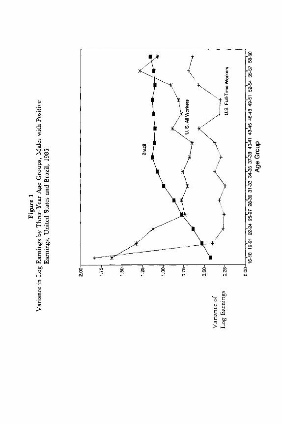
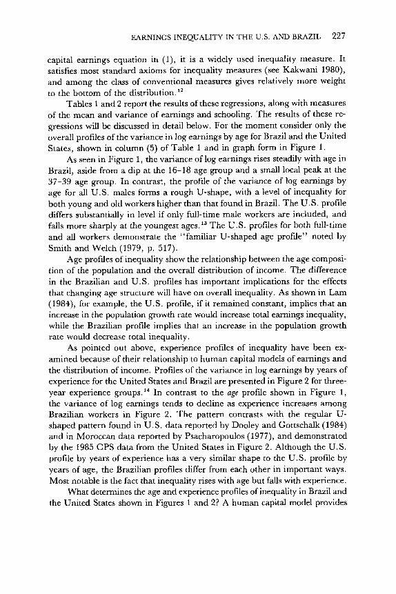
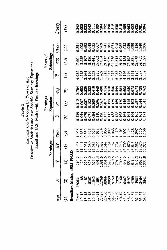
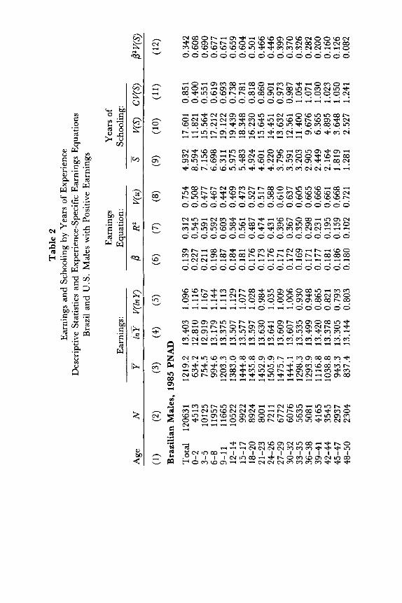
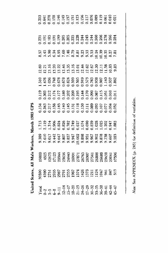
Tables 1 and 2 report the results of these regressions, along with measures of the mean and variance of earnings and schooling. The results of these regressions will be discussed in detail below. For the moment consider only the overall profiles of the variance in log earnings by age for Brazil and the United States, shown in column (5) of Table 1 and in graph form in Figure 1.

As seen in Figure 1, the variance of log earnings rises steadily with age in Brazil, aside from a dip at the 16-18 age group and a small local peak at the 37-39 age group. In contrast, the profile of the variance of log earnings by age for all U.S. males forms a rough U-shape, with a level of inequality for both young and old workers higher than that found in Brazil. The U.S. profile differs substantially in level if only full-time male workers are included, and falls more sharply at the youngest ages.I3 The U.S. profiles for both full-time and all workers demonstrate the “familiar U-shaped age profile” noted by Smith and Welch (1979, p. 517).

Age profiles of inequality show the relationship between the age composition of the population and the overall distribution of income. The difference in the Brazilian and U.S. profiles has important implications for the effects that changing age structure will have on overall inequality. As shown in Lam (1984), for example, the U.S. profile, if it remained constant, implies that an increase in the population growth rate would increase total earnings inequality, while the Brazilian profile implies that an increase in the population growth rate would decrease total inequality.

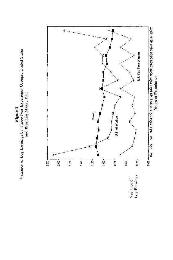
As pointed out above, experience profiles of inequality have been ex- amined because of their relationship to human capital models of earnings and the distribution of income. Profiles of the variance in log earnings by years of experience for the United States and Brazil are presented in Figure 2 for three- year experience groups.14 In contrast to the age profile shown in Figure 1, the variance of log earnings tends to decline as experience increases among Brazilian workers in Figure 2. The pattern contrasts with the regular U- shaped pattern found in U.S. data reported by Dooley and Gottschalk (1984) and in Moroccan data reported by Psacharopoulos (1977), and demonstrated by the 1985 CPS data from the United States in Figure 2. Although the U.S. profile by years of experience has a very similar shape to the U.S. profile by years of age, the Brazilian profiles differ from each other in important ways. Most notable is the fact that inequality rises with age but falls with experience.

What determines the age and experience profiles of inequality in Brazil and the United States shown in Figures 1 and 2? A human capital model provides

bJl

3 E: .-


a useful framework for decomposing the determinants of these profiles. We estimate the conventional earnings equation in (5) for separate age and experience groups in an attempt to identify variations across age and experience in components such as the returns to schooling, the variance in schooling, and unexplained residual variance.

Decomposing Age Pro$les

Consider first the variance of log earnings, the variance of residuals, and the coefficient of determination (R’) from earnings regressions using separate three-year age groups. These estimates are shown in columns 5 , 7, and 8 of Table 1. The results make it possible to decompose the total variance into the “explained” and “unexplained” portions from the simple log-linear earnings equation. “Explained” variance, PVCS,, is shown in column 12 of Table 1. The most dramatic difference in the results for the two countries is the much higher values of R’ in Brazil. For the United States, R2 is typically between 10 and 15 percent, never exceeding 18 percent. For Brazil, R2 is typically over 40 percent in the prime working ages.

In the United States regressions the profile of residual variance by age closely follows the profile of total variance. In Brazil residual variance rises with age, but rises noticeably less steeply than does total variance up to the age group 37-39. The sharp increase in total variance between ages 16 and 37 in Brazil is primarily due to a sharp increase in “explained variance.” As seen in column 12 of Table 1, explained variance, p2V(S), increases up to this age group, then falls steadily for older age groups.

As demonstrated previously, an important determinant of cross-sectional age profiles of inequality is differences in schooling distributions across age groups. The mean, variance, and coefficient of variation of years of schooling in the two countries are shown in columns 9, 10, and 11 of Table 1. Column 9 of Table 1 shows the large difference in mean schooling between the two countries, a difference of seven to nine years for almost all age groups. Both countries dis- play rising mean schooling over time, recognizing that the youngest cohorts have not completed schooling and thus exclude students not in the labor force.

The most important features of these schooling distributions are the differences in the level and shape of the variance of schooling profiles. The U.S. male cohorts have experienced a steady decline in schooling variance during the last thirty years. Brazilian male cohorts, on the other hand, experienced an increase in schooling variance, at least up to the cohorts who were aged 37-39 in 1985. The variance in schooling for these cohorts in their late thirties

’ in 1985 is more than twice as high as the variance in schooling at the same ages in the United States, in spite of the fact that mean schooling is well over twice as high in the United States at these ages. Reading the age profile in Table 1 as a time series of cohort schooling histories, dramatic increases in

Tab

le 1

E

arni

ngs

and

Scho

olin

g by

Yea

rs o

f A

ge

Des

crip

tive

Stat

istic

s an

d A

ge-S

peci

fic E

arni

ngs

Equ

atio

ns

Bra

zil a

nd U

.S.

Mal

es w

ith P

ositi

ve E

arni

ngs

Ear

ning

s Y

ears

of

Ear

ning

s:

Equ

atio

n:

Scho

olin

g:

- s

V(S)

CV

(S)

pV(s

) -

Age

N

Y

tFY

V(l

nv

6 R’

V(

u)

(1)

(2)

(3)

(4)

(5)

Bra

zilia

n M

ales

, 19

85 PNAD

Tot

al

10-1

2 13

-15

16-1

8 19

-21

22-2

4 25

-27

28-3

0 31

-33

34-3

6 37

-39

40-4

2 43

-45

46-4

8 49

-51

52-5

4 55

-57

58-6

0

1206

3 1

1188

41

87

8367

1 1

045

1169

1 11

769

1096

6 10

030

9159

79

28

7160

65

67

5497

47

89

3983

34

64

2841

1219

.2

128.

1 22

6.2

356.

0 57

3.1

801.

3 10

81.6

13

31.5

15

78.3

16

70.5

17

91.3

17

09.4

16

41.2

16

64.4

16

11.1

15

42.3

13

63.7

13

33.8

13.4

03

11.4

44

12.0

81

12.5

80

12.9

83

13.2

55

13.4

82

13.6

47

13.7

54

13.7

57

13.7

81

13.7

48

13.7

00

13.6

70

13.6

43

13.5

87

13.4

70

13.3

77

1.09

6 0.

688

0.56

0 0.

426

0.52

9 0.

638

0.77

4 0.

866

0.98

9 1.

068

1.12

9 1.

103

1.09

7 1.

114

1.12

8 1.

097

1.11

0 1.

156

0.13

9 0.

044

0.07

9 0.

071

0.09

4 0.

110

0.12

6 0.

135

0.14

7 0.

155

0.15

8 0.

163

0.16

4 0.

164

0.16

4 0.

165

0.16

1 0.

171

0.31

2 0.

007

0.05

7 0.

102

0.20

9 0.

296

0.36

7 0.

407

0.45

5 0.

479

0.46

9 0.

470

0.44

6 0.

416

0.40

2 0.

387

0.34

4 0.

341

0.75

4 0.

683

0.52

9 0.

383

0.41

9 0.

449

0.49

0 0.

514

0.54

0 0.

556

0.59

9 0.

585

0.60

8 0.

650

0.67

5 0.

672

0.72

8 0.

762

4.93

2 1.

518

3.26

4 4.

496

5.55

8 5.

935

5.96

2 5.

943

5.83

5 5.

276

5.03

5 4.

498

4.12

6 3.

926

3.73

1 3.

425

3.09

7 2.

802

17.6

01

2.32

8 5.

107

8.48

6 12

.441

15

.663

17

.854

19

.417

20

.939

21

.236

21

.343

19

.491

18

.155

17

.198

16

.821

15

.678

14

.755

13

.397

0.85

1 1.

005

0.69

2 0.

648

0.63

5 0.

667

0.70

9 0.

741

0.78

4

0.91

8 0.

982

1.03

3 1.

056

1.09

9 1.

156

1.24

0 1.

306

0.87

3

(12)

0.34

2 0.

005

0.03

2 0.

043

0.11

1 0.

189

0.28

4 0.

352

0.45

0 0.

512

0.53

0 0.

518

0.48

9 0.

463

0.45

3 0.

425

0.38

1 0.

394

Uni

ted

Stat

es, A

ll M

ale

Wor

kers

, M

arch

198

5 CPS

Tot

al

3059

0 13

-15

343

16-1

8 17

39

19-2

1 23

86

22-2

4 26

71

25-2

7 28

08

28-3

0 28

52

31-3

3 26

46

34-3

6 24

26

37-3

9 22

10

40-4

2 18

16

43-4

5 15

42

46-4

8 13

09

49-5

1 12

46

52-5

4 12

12

55-5

7 11

62

58-6

0 10

34

1980

0 67

5 18

49

5928

10

633

1594

4 19

669

2221

9 24

299

2758

5 28

233

2882

9 27

658

2719

3 27

591

2648

8 25

423

9.38

9 5.

819

6.90

7 8.

204

8.89

2 9.

418

9.63

5 9.

770

9.85

9 9.

995

10.0

25

10.0

00

9.97

4 9.

950

9.95

3 9.

854

9.82

3

1.71

3 1.

623

1.62

2 1.

322

1.12

3 0.

736

0.77

7 0.

703

0.75

9 0.

676

0.64

4 0.

886

0.81

3 0.

907

1.28

4 1.

069

0.78

0

0.15

4 0.

146

0.16

7 - 0

.014

-

0.01

1

0.06

5 0.

080

0.09

9 0.

107

0.11

0 0.

098

0.11

4 0.

115

0.11

6 0.

094

0.08

3 0.

110

0.11

9 0.

007

0.03

4 0.

000

0.00

1 0.

036

0.05

8 0.

106

0.12

3 0.

156

0.14

6 0.

145

0.17

4 0.

174

0.11

4 0.

069

0.14

2

1.51

0 1.

611

1.56

8 1.

321

1.12

2 0.

709

0.73

1 0.

629

0.66

5 0.

571

0.55

0 0.

757

0.64

4 0.

671

0.80

4 1.

196

0.91

7

12.6

9 8.

43

10.3

3 12

.08

12.6

9 12

.97

13.2

4 13

.36

13.5

5 13

.61

13.2

6 12

.95

12.7

0 12

.52

12.4

5 12

.12

11.8

8

8.57

0.

56

1.96

2.

90

5.35

6.

30

7.13

7.

58

8.22

8.

74

9.84

9.

99

10.3

5 10

.44

11.7

4 12

.71

12.5

7

0.23

1 0.

089

0.13

5 0.

141

0.18

2 0.

193

0.20

2 0.

206

0.21

2 0.

217

0.23

7 0.

244

0.25

3 0.

258

0.27

5 0.

294

0.29

8

0.20

3 0.

012

0.05

5 0.

001

0.00

1 0.

027

0.04

6 0.

074

0.09

4 0.

106

0.09

5 0.

130

0.13

7 0.

140

0.10

4 0.

088

0.15

2

Note

: Se

e A

PPE

ND

IX (

p. 2

45)

for

defi

nitio

n of

var

iabl

es.

Tab

le 2

E

arni

ngs

and

Scho

olin

g b

y Y

ears

of

Exp

erie

nce

Des

crip

tive

Stat

istic

s an

d E

xper

ienc

e-Sp

ecif

ic E

arni

ngs

Equ

atio

ns

Bra

zil a

nd U

.S.

Mal

es w

ith P

ositi

ve E

arni

ngs

Ear

ning

s Y

ears

of

Ear

ning

s:

Equ

atio

n:

Scho

olin

g:

-

-

N

Y In

Y V(

1nY)

B

R2

V(u)

s

V(S)

C

V(S)

pv

(s)

Age

(1)

(2)

(3)

(4)

(5)

Bra

zilia

n M

ales

, 19

85 P

NA

D

Tot

al

0-2

3-5

6-8

9-1

1 12

-14

15-1

7 18

-20

21-2

3 24

-26

27-2

9 30

-32

33-3

5 36

-38

39-4

1 42

-44

45-4

7 48

-50

1206

3 1

4513

10

125

1195

7 1 1

665

1052

2 99

22

8924

80

0 1

721 1

67

72

6076

56

35

508 1

41

65

3545

29

37

2304

1219

.2

634.

2 75

4.5

994.

6 12

03.3

13

83.0

14

44.8

14

35.8

14

52.9

15

05.9

14

75.7

14

44.1

12

98.3

12

93.9

11

16.8

10

38.8

94

3.3

837.

4

13.4

03

12.8

10

12.9

19

13.1

79

13.3

75

13.5

07

13.5

77

13.5

97

13.6

30

13.6

41

13.6

09

13.6

07

13.5

35

13.4

99

13.4

20

13.3

78

13.3

05

13.1

44

1.09

6 1.

116

1.16

7 1.

144

1.11

3 1.

129

1.07

7 1.

028

0.98

4 1.

035

1.00

9 1.

006

0.93

0 0.

948

0.86

5 0.

821

0.79

3 0.

803

0.13

9 0.

227

0.21

1 0.

198

0.18

7 0.

184

0.18

1 0.

176

0.17

3 0.

176

0.17

1 0.

172

0.16

9 0.

171

0.17

7 0.

181

0.18

6 0.

180

0.31

2 0.

545

0.59

1 0.

592

0.60

3 0.

584

0.56

1 0.

487

0.47

4 0.

431

0.39

6 0.

367

0.35

0 0.

298

0.23

1 0.

195

0.15

9 0.

102

0.75

4 0.

508

0.47

7 0.

467

0.44

2 0.

469

0.47

3 0.

527

0.51

7 0.

588

0.61

0 0.

637

0.60

5 0.

665

0.66

6 0.

661

0.66

8 0.

721

4.93

2 8.

594

7.15

6 6.

698

6.31

1

5.97

5 5.

483

4.92

4 4.

601

4.22

0 3.

796

3.59

1 3.

203

2.90

5 2.

449

2.16

4 1.

819

1.28

1

17.6

01

11.8

21

15.5

64

17.2

12

19.1

22

19.4

39

18.3

48

16.2

30

15.6

45

14.4

51

13.6

32

12.5

61

11.4

00

9.67

6 6.

365

4.89

5 3.

648

2.52

7

0.85

1 0.

400

0.55

1 0.

619

0.69

3 0.

738

0.78

1 0.

818

0.86

0 0.

901

0.97

3 0.

987

1.05

4 1.

071

1.03

0 1.

023

1.05

0 1.

241

(12)

0.34

2 0.

608

0.69

0 0.

677

0.67

1 0.

659

0.60

4 0.

501

0.46

6 0.

446

0.39

9 0.

370

0.32

6 0.

282

0.20

0 0.

160

0.12

6 0.

082

Uni

ted

Stat

es, A

ll M

ale

Wor

kers

, Mar

ch 1

985

CPS

Tota

l 0-

2 3-

5 6-

8 9-

1 1

12-1

4 15

-17

18-2

0 21

-23

24-2

6 27

-29

30-3

2 33

-35

36-3

8 39

-41

42-4

4 45

-47

3059

0 43

90

2751

29

35

2987

27

91

2355

19

87

1574

14

26

1373

12

11

1124

10

47

941

847

513

1980

0 45

25

1267

5 17

123

2034

4 23

636

2494

0 26

991

2787

1 26

765

2690

7 27

541

2680

8 26

688

2343

8 20

041

1759

6

9.38

9 7.

610

9.01

7 9.

442

9.64

7 9.

807

9.85

7 9.

947

10.0

02

9.89

8 9.

951

9.96

7 9.

902

9.87

8 9.

738

9.60

7 9.

283

1.71

3 2.

119

1.31

4 0.

906

0.82

4 0.

826

0.78

2 0.

749

0.62

7 1.

074

0.69

0 0.

839

1.02

8 1.

025

1.20

2 0.

947

1.88

3

0.15

4 0.

343

0.21

7 0.

158

0.14

5 0.

140

0.14

5 0.

131

0.11

8 0.

130

0.11

1 0.

089

0.09

3 0.

107

0.07

7 0.

034

0.05

2

0.11

9 0.

303

0.21

2 0.

174

0.17

7 0.

180

0.20

2 0.

200

0.19

5 0.

144

0.17

0 0.

090

0.08

7 0.

115

0.05

1 0.

010

0.01

1

1.51

0 1.

476

1.03

6 0.

748

0.67

8 0.

678

0.62

4 0.

599

0.50

5 0.

919

0.57

3 0.

763

0.93

8 0.

907

1.14

0 0.

937

1.86

2

12.6

9 12

.21

13.1

6 13

.20

13.2

2 13

.46

13.3

5 13

.16

13.0

1 12

.44

12.6

2 12

.67

12.3

0 12

.11

11.5

8 10

.83

9.83

8.57

5.

45

5.90

6.

34

6.95

7.

60

7.48

8.

79

8.81

9.

23

9.53

9.

53

10.2

4 10

.39

10.3

5 8.

27

7.81

0.23

1 0.

191

0.18

5 0.

191

0.19

9 0.

205

0.20

5 0.

225

0.22

8 0.

244

0.24

5 0.

244

0.26

0 0.

266

0.27

8 0.

266

0.28

4

0.20

3 0.

641

0.27

8 0.

158

0.14

6 0.

149

0.15

7 0.

151

0. I2

3 0.

156

0.11

7 0.

076

0.08

9 0.

119

0.06

1 0.

010

0.02

1

Not

e: S

ee A

PPE

ND

IX (

p. 2

45)

for

defin

ition

of

varia

bles

.


the variance in schooling of cohorts occurred in Brazil for cohorts being educated during the 1940s, 1950s, and into the 1960s. An inspection of columns 9, 10, and 11 of Table 1 clearly points out that this sharp increase in the variance in schooling was attributable to the steady increase in mean schooling. In fact, column 11 shows that the coefficient of variation in years of schooling falls from older cohorts to younger cohorts, demonstrating that for this mean-adjusted measure at least, inequality in schooling in Brazil has declined as the overall level of schooling has increased.

The variance in schooling in Brazil may have begun to decline, beginning with cohorts who were in their late thirties in 1985. Specifically, the variance in years of schooling peaks with the cohorts aged 34-36 and 37-39 in 1985, that is, the cohorts born between 1946 and 1951. Since these cohorts are old enough to have completed their schooling in 1985, it seems unlikely that this decline is an artifact of the younger ages. The importance of this decline on earnings inequality can be seen by referring to the decomposition of the variance of log earnings (Table 1). The R2 hits a peak at the 34-36 age group, a result not due to Mincer-type post-schooling human capital effects, but rather to the peak in the variance of schooling at this age. Residual variance, which picks up the effects of returns to post-schooling human capital investments, rises monotonically from age 16-19. The sharp decline in schooling variance for successively younger cohorts that begins around age 34 is asso- ciated with declines in both R2 and in total variance for the same cohorts. While not conclusive, the results are suggestive of a trend toward decreasing earnings inequality in Brazil, a direct result of decreasing variance in schooling. Such an effect-declining earnings inequality as a result of declining variance in schooling-is consistent with the predictions of Becker and Chiswick (1966) and Chiswick (1971).

If returns to schooling were constant across age groups, the variance in schooling would completely determine the “explained” or between-group component of total variance in log earnings. Inspection of column 6 of Table 1 demonstrates that these returns are not constant, however, in either the United States or Brazil. Abstracting from the initial decline in fi with age in the United States, presumably reflecting the presence of students with part-time earnings, there is a tendency for returns to schooling to rise with age in both countries. l 6

The results also show consistently higher returns to schooling in Brazil. The estimated returns to schooling in Brazil are higher by around five percentage points than returns to schooling in the United States for almost every age group. These higher returns in Brazil might be considered consistent with Langoni’s (1973) argument that apparent increases in inequality in Brazil

EARNINGS INEQUALITY IN T H E U.S. AND BRAZIL 235

during the 1960s and 1970s were due to quasi-rents to human capital resulting from Brazil’s rapid (and presumably unexpected) economic growth. Signifi- cantly higher returns to schooling for developing countries than for developed countries have often been estimated, however, and the .15 to .18 rates of return estimated in Brazil are consistent with estimates in other developing countries (Psacharopoulos 1981 ; Heckman and Hotz 1986). While the fairly rapid increase in the mean level of schooling discussed above might be expected to reduce returns to schooling, the effect of these changes on the shape of the age profile of returns depends on interactions between returns to schooling and returns to experience that simply cannot be identified in a single cross section.

Since the explained variance in (5) is pV(S), the increase in returns to schooling with age in both the United States and Brazil has the effect of par- tially offsetting the decline in the variance of schooling with age. As seen in column 12 of Table 1, the net effect is that explained variance is relatively constant across age groups in both countries from about age 34. In Brazil this means that the rising inequality and falling R2 from age 34 are attributable to residual variance, including returns to post-schooling human capital as well as all other components of earnings uncorrelated with schooling.

Comparing age-specific earnings equations for U. S. and Brazilian males, it can be seen that the two components of explained variance in log earnings, that is, returns to schooling and the variance in schooling, are both substantially higher in Brazil than in the United States. The importance of these differences can be seen by comparing the values of PVCS, for the United States and Brazil in column 12 of Table 1. Considering the 31-33 age group, for example, explained variance is only .074 in the United States compared to .450 in Brazil. If the U.S. sample is restricted to full-time workers, explained variance falls to .038. Residual variance differs greatly between all workers and full-time workers for the U.S. sample, .629 for all males compared to only .208 for full-time males in the 31-33 age group, but both end up with lower total variance than the Brazilian 31-33 year-old males.

The fact that a simple human capital model appears to have so much greater explanatory power in Brazil than in the United States is often surpris- ing to those unfamiliar with data on earnings and schooling from developing countries. The results should be qualified by well-known warnings that the coefficient on schooling includes the effects of many omitted variables corre- lated with schooling. It is often argued that in Brazil, as in many developing countries, high levels of schooling are much more concentrated among the children of wealthy families than they are in the United States, so that schooling may partly serve as a proxy for status and family connections.”


Decomposing Experience ProJles

As pointed out in previous sections, experience profiles of inequality may differ greatly from age profiles of inequality, especially when both cohort sizes and schooling distributions differ significantly across cohorts. As shown in Figures 1 and 2, although the age and experience profiles for the United States are quite similar, the age and experience profiles for Brazil actually move in opposite directions. Given the importance of years of experience in human capital models of earnings, it is instructive to examine the components of experience profiles of earnings inequality in the United States and Brazil, presented in detail in Table 2.

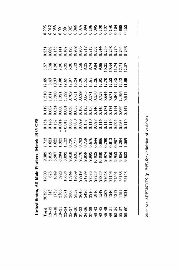
Columns 5, 7, and 8 of Table 2 show the total log variance, the residual variance, and RZ as a function of experience when earnings equation (5) is estimated for separate three-year experience groups in the United States and Brazil. The relationship between experience and both the coefficient of determination (R2) and the variance of residuals are consistent with the Moroccan results of Psacharopoulos (1977) and with Mincer’s prediction of a peak in RZ and a trough in residual variance at the overtaking point. Residual variance has a trough around 9-11 years of experience, and R2 has a peak at around the same point.

The U.S. profiles are more U-shaped than the Brazilian profiles, and demonstrate the much lower R2 that were seen in the age profiles above. Like Brown (1980), we find mixed evidence in the U.S. experience profiles for an overtaking point. For the all-worker sample, both residual variance and total variance do not reach a trough until over twenty years of experience, well beyond standard predictions of an overtaking point.

Similar to the finding that a human capital earnings equation has several times more explanatory power in Brazil than in the United States, it is sur- prising to find that the Brazilian profiles of inequality by experience give more support to Mincer’s predictions than do U.S. profiles. There appears to be support for an overtaking point around 9- 11 years of experience in the Bra- zilian profile of RZ and residual variance. Many factors, including changes in cohort size and schooling distributions, are reflected in these cross-sectional profiles in addition to effects of post-schooling human capital investments and “overtaking.” Neither the U.S. nor the Brazilian patterns provide a con- vincing test of Mincer’s predictions.

A purer test of Mincer’s predictions is provided by analysis of experience profiles of the variance in log earnings for separate schooling categories. The variances of log earnings corresponding to the within-group variances ui&) in equation 4 show that three schooling groups, those with zero years, 1-4 years, and 5-8 years (accounting for the vast majority of workers in every experience


group), have inequality profiles that are consistent with an overtaking point in the range of 3-12 years of experience. For men with zero schooling and 1-4 years of schooling the variance in log earnings reaches a global minimum after 9-1 1 years of experience, rising at a fairly constant rate thereafter. For men with 5-8 years of schooling, the trough occurs at 3-5 years of experience. The inequality profile for the men with 9-1 1 years of schooling shows no evidence of an “overtaking point,” tending to rise monotonically with experience. Such a pattern can be explained in terms of post-schooling investments in human capital if there is a positive correlation between “initial earnings capacity” and on-the-job training. It is interesting to note that Mincer found the same positive relationship between log variance of earnings and experience for higher schooling groups in the United States (1974, p. 103-105).

Recalling the pattern in overall log variance for all schooling groups combined, it is interesting to note that total variance falls with experience in Brazil at the same time that the variance for every separate schooling group rises with experience. Two factors in the decomposition of total variance provide the principle explanation for this phenomenon. First, within-group variance in (4) is a weighted average of schooling-specific profiles and the weights give increasingly more importance to the zero schooling group as experience increases, a result of the secular increase in schooling in Brazil. Since the profile for the zero schooling group is relatively flat, the combined within-group variance rises more slowly with experience than any of the profiles for non-zero schooling groups. The second part of the explanation is provided by our decomposition of experience-specific earnings equations in Table 2. While within-group (residual) variance rises with experience, between-group (explained) variance falls with experience because of the rapid decline in the variance of schooling. It is the latter effect that dominates in the Brazilian experience profile of total log variance.

Comparison of Age and Experience Profiles

As noted, the U.S. experience profile of inequality exhibits a U-shape very similar to the U.S. age profile of inequality. For Brazil, however, the age and experience profiles of earnings inequality differ in important ways. Most notably, inequality rises with age in Brazil, but falls with experience beginning at 3-5 years. The key to this discrepancy lies in the relative strengths of residual (unexplained) variance and explained variance of log earnings by age and experience. The decompositions indicate that in Brazil the residual variance rises with age. A similar pattern can be detected when the residual variance is calculated by experience (see column 12, Tables 1 and 2). The coefficient of determination, reflecting both explained variance and total


variance, is an inverted U in both profiles, but falls more rapidly with experience than with age. The explanation for the fact that inequality falls with experience is that explained variance, pV(S), falls rapidly with experience but is almost constant with age. In Tables 1 and 2, several comparisons help clarify this. First, the variance in years of schooling, V(S), falls rapidly with experience, but falls more slowly with age once it peaks at ages 31-33. Second, returns to schooling, b, tend to be higher in experience groups than in age groups and tend to fall with experience but to rise with age. The net effect of these differences is that explained variance, shown in column 12, falls fast enough as a function of experience to offset the increase in residual variance, leading to a net decline in total variance as a function of experience. Explained variance does not fall fast enough with age to offset the increase in residual variance, leading to an increase in total variance as a function of age. The difference in the shape of these cross-sectional profiles in the U.S. and Brazil does not necessarily reveal any fundamental difference in the relationship between experience and earnings in the two countries. Both profiles are affected by the specific features of historical changes in schooling distributions and cohort sizes in the two countries.

Alternative Definitions of Experience in Brazil

Identifying labor market experience is always problematic in the estima- tion of earnings equations. Ideally we would like to have direct data on years of work experience or the age at which full-time work began. In the absence of such data the standard proxy is Experience =Age - Schooling - 7, used in our estimates above. This assumes a once-and-for-all clearly defined transition from school to work and assumes no unemployment or underemployment, known to be high in developing countries. The problem is especially serious in a country like Brazil, where many end their formal schooling while still children. There is a difficult question of when work experience can really be considered an addition to human capital. For example, do seven-year-old children washing car windows in Brazil increase their human capital from their labor market experience?

The imputation of labor market experience in Brazil has been an issue in estimates of the returns to schooling in Brazil. Behrman and Birdsall (1983, 1985) have argued that effective adult labor market experience does not begin until age 15 and have truncated all experience at that point. Eaton (1985) has criticized their approach and argued for a conventional definition, such as the one we have used in Table 2. In the absence of strong prior knowledge of the correct definition of experience, the researcher is faced with choosing between one kind among several selection biases. In the Brazilian data, earnings are not reported for children under ten, but the standard experience imputation


will assign years of experience to many workers for years when they were younger than ten. The result is that the zero experience group under the standard definition excludes all workers with less than three years of schooling, a large portion of the sample. The Behrman and Birdsall definition, on the other hand, excludes all work prior to age 15, and thus makes the lowest experience groups systematically larger and less schooled than they would be under the standard definition.

The magnitude of the biases in Brazil can be demonstrated by comparing the size and characteristics of the 0-2 experience group under alternative definitions. We have reestimated our results using two alternative definitions of labor market experience, one assuming that effective labor market experience begins at age 10 and the second at age 15. When the “standard” definition E = A - S - 7 is used, there are 4,513 males with 0-2 years of experience, as shown in Table 2, with mean schooling of 8.6 years. When Behrman and Birdsall’s definition E = min[(A - S - 7), (A - 15)] is used, there are 12,574 males with 0-2 years of experience, with mean schooling of 4.8 years. Estimated returns to schooling in the 0-2 experience group fall from .23 with the standard definition to .14 with the Behrman-Birdsall definition. Turning to the experience profiles of log variance, R2, and residual variance, the alternative definition makes a substantial difference in the first experience groups, but has little effect thereafter. Total log variance in earnings for the 0-2 year experience group drops from the 1.1, shown in Table 2, to -85 and changes its initial direction from increasing to decreasing. Similar results occur with R’, which falls from .54 for the 0-2 year experience group under the standard definition to .36 under the Behrman-Birdsall definition. The explanation for the significantly lower variance in log earnings for the 0-2 year experience group under the Behrman-Birdsall definition is that the 8,000 workers with little or no schooling who are added to the original 4,513 make up a group sufficiently large and homogeneous to reduce earnings variance in the group.

Rural- Urban and Regional Variations in Brad

Given high levels of migration and large regional differences existing in Brazil, it is natural to wonder if inequality profiles vary systematically across regions or between rural and urban areas. For example, if urban populations tend to be younger due to in-migration of young adults, then the age profiles of inequality may in part pick up regional income disparities. In order to test the robustness of the Brazilian results and their applicability to different strata within Brazil, earnings equation (5) was estimated for two very different regions of Brazil, the Northeast and the Southeast. A further rural-urban stratification was done for these two regions and for Brazil as a whole. The


southeast region was represented by the states of Rio de Janeiro and ,550 Paulo, representing the richest and most developed parts of Brazil. In contrast, the northeast region is one of the poorest parts of Brazil, and has lagged behind the southeast region in virtually all indicators of economic development."

The sample is large enough that it is possible to analyze separate three- year age groups in the urban Southeast and the rural Northeast regions and maintain reasonable cell sizes. As expected, very large regional differences in mean schooling and earnings are found, with mean earnings almost four times higher in the urban Southeast than in the rural Northeast. Mean schooling ranges from 1 . 3 years in the rural Northeast to 6.3 years in the urban South- east. Surprisingly, in spite of these substantial differences in the levels of schooling and earnings, the age and experience profiles of inequality in general show patterns in different regions that are remarkably similar to those for Brazil as a whole. The overall level of inequality tends to be lower for specific regions than for Brazil as a whole, an expected (though not required) result given the large inter-regional variations in earnings. Only in the rural Northeast, however, is inequality substantially lower in every age group. This is explained primarily by the much lower variance in schooling in the rural Northeast where the age profile of earnings inequality is also considerably flatter than the profile for other areas. It is impossible to identify whether this different shape of the inequality profile occurs because the secular increases in schooling levels typical of the rest of Brazil have not occurred in the rural Northeast or because of out-migration selective of the best-educated younger workers.

The regional comparisons show surprisingly similar patterns in returns to schooling for all age and experience groups. The returns to schooling estimated for all age groups combined are almost identical in the urban Southeast and rural Northeast, in spite of the vast differences in the mean levels of schooling and earnings. Profdes of R2 by age and experience have similar shapes across regions of Brazil, but levels of RZ are much lower in rural areas, especially in the rural Northeast. Thus, although our estimates of returns to schooling are similar in urban and rural areas, the differences in years of schooling in rural areas explain much less of the variance in earnings. Residual variance is only slightly lower in the rural Northeast, so that the much lower explained variance leads to a very low R2, a frequently observed result in earnings equations for rural samples.

On the whole, the basic patterns in the age and experience profiles of earnings inequality for all of Brazil appear remarkably robust across regions, in spite of the large differences in the overall levels of schooling and earnings in these regions.


Conclusion

This study documents age and experience profiles of earnings inequality for Brazilian and U.S. males and decomposes those profiles using a human capital framework. The analysis reveals a number of important facts about cross-sectional inequality profiles and the determinants of inequality in the two countries. While the U.S. experience profie of inequality exhibits a U- shape very similar to the U.S. age profile of inequality, the age and experience profiles of earnings inequality for Brazil differ from each other in important ways, with neither profile exhibiting the U-shape characteristic in the United States. The consistency between the shapes of the age and experience profiles of inequality is thus not a universal tendency, but depends on age and schooling distributions.

Looking at the specific components of the variance of log earnings, we find the following:

1. Returns to schooling: We estimate significantly higher returns to schooling in Brazil than in the United States, consistent with previous comparisons of less developed and industrialized countries. This result holds for every three-year age group over age 19, with the difference typically exceeding five percentage points at every age. 2. Variance in years of schooling: The variance in schooling differs greatly across age and experience groups in both the United States and Brazil and plays a central role in explaining both the shape of the profiles in the two countries and the differences between the countries. Brazil experienced increasing variance in schooling across male cohorts for many years, at the same time that the variance in schooling was declining in the United States. In the most extreme case, the variance in schooling is almost twice as high in Brazil, in spite of a mean level of schooling only a fourth of that of the United States. This trend appears to have peaked in Brazil, leading to lower inequality for younger cohorts. 3 . Residual Variance: Residual variance is significantly higher in the United States than in Brazil. Evidence on Mincer’s predictions of an ‘‘overtaking point” in experience profiles of residual variance is stronger for Brazil than for the United States, with a trough at 9-11 years of experience in Brazil contrasting with a trough at 21-23 years in the United States. Together these results suggest that a simple human capital earnings equa-

tion has substantially larger explanatory power for almost all age groups in Brazil than in the United States, with RZ from two to four times higher in Brazil. Most of the results are robust to regional and rural-urban stratification. Some sensitivity is found, however, to the choice of proxy for labor market experience.


The results confirm the importance of using caution in the interpretation of cross-sectional profiles of earnings and inequality. Predictions based on cohort profiles can be confounded in cross sections by variations in schooling distributions and cohort sizes across age and experience groups. These effects play an important role in explaining inequality profiles in both the United States and Brazil, but are especially critical in Brazil due to the rapid changes in schooling distributions over time.

ENDNOTES

‘This article has benefited from the comments of Ricardo Paes de Barros, Guilherme Sedlacek, JosC Guilherme Almeida dos Reis, and Charles Brown. Excellent research assistance was provided by Robert Schoeni. Support from the Fulbright Commission, the Program for International Partnerships of the University of Michigan, and the Instituto de Planejamento Econamico e Social - IPENINPES, Rio de Janeiro, is gratefully acknowledged.

‘See, for example, Paglin (1975), Schultz (1975), Morley (1981), and Lam (1984), for a discussion of the relationship between age structure and inequality.

‘See Mincer (1974, pp. 19-21) and Brown (1980). 3Post-schooling human capital refers to investments such as on-the-job training that have

direct or opportunity costs in the form of foregone earnings. Returns to experience per se are not included.

4Psacharopoulos and Layard (1979) are especially critiral of this assumption. ’If the present value of lifetime wages with post-schooling human capital investments is

equal to the present value of lifetime wages with no such investments, then a simple model with constant returns to post-schooling investments rP and constant opportunity costs will imply an overtaking point j = lhD. The typical prediction is that j will be something less than ten years (Mincer 1974; Brown 1980).

6The U-shaped profile V(1nY) will be altered by any non-zero correlation between post- school investments and either initial earnings capacity or the level of schooling, with any shape possible in principle.

’See Mincer (1974), Schultz (1975), and Smith and Welch (1979). ‘This is abstracting from mortality and migration, which may differ substantially across

schooling groups. We also abstract from additional formal schooling acquired after entering the labor force, such as evening classes.

’An age cross section refers to a profile of inequality by age in a population at a single point in time.

‘This implies that the labor force growth rate must be zero, with a uniform age distribution. “Results for Brazil are derived from the 1985 Pesquisu Nacional por Amostra de Domicilios

(PNAD), the annual household survey conducted by the Instituto Brasileiro de Geografia e Estatistzca (IBGE). The results reported here use the weights included in the data set by IBGE to produce a representative sample of the Brazilian population. The 1985 data give monthly labor earnings. Whereas we report sample sizes, they refer to the unweighted number of observations. U.S. results are based on the March 1985 Current Population Survey. The CPS data give annual rather than monthly earnings.

”As shown by Atkinson (1970), the ordering of distributions implied by the log variance is consistent with a higher degree of “relative inequality aversion” than is implied by other standard measures such as the Gini coefficient and the coefficient of variation


Womparison of total log variance for full-time and all-worker samples reveals the sensitivity of total inequality in the United States to the choice of full-time versus all-worker samples. The all-worker U.S. sample has significantly higher inequality than the Brazilian sample overall, although this is hardly ever true for specific age groups. The full-time U.S. sample has significantly lower inequality than the Brazilian sample.

I4For the United States, experience is defined as age minus years of schooling minus six. For Brazil, experience is defined as age minus years of schooling minus seven. The seven-year beginning age for schooling is consistent with distributions of school attendance by age reported in Haussman and Haar (1978). Imputing experience is difficult in a country such as Brazil in which a large percentage of the population have only a few years of schooling. In other results we have alternatively assumed that work does not begin until age 10 or age 15, the latter approach being preferred by Behrman and Birdsall (1983).

”We recognize that we are abstracting from many historical and institutional determinants of inequality, particularly in regard to the large regional variations in inequality in Brazil. We have repeated our analysis for separate regions of Brazil and for rural and urban samples.

16A dramatic effect of the presence of students with part-time earnings in the sample is negative returns to schooling estimated for age groups 19-21 and 21-24 in Table 1. This is one of a number of examples of the sensitivity of the U.S. results to the fact that many men do not complete schooling until their early twenties. In Brazil, in contrast, very few men are still in school at these ages.

”Behrman and Wolfe (1984) conclude from evidence on siblings in Nicaragua that estimates of returns to schooling are significantly overstated when family-related background characteristics are not controlled.

‘‘We used the PNAD definition of the Northeast, consisting of the states of Alagoas, Bahia, Ceara, MaranhHo, Paraiba, Pernambuco, Piaui, Rio Grande do Norte, and Sergipe.

REFERENCES

Atkinson, Anthony B. 1970. “On the Measurement of Inequality.” Journal of Economic Theory

Becker, Gary S., and Barry R. Chiswick. 1966. “Education and the Distribution of Earnings.”

Behrman, Jere R . , and Nancy Birdsall. 1983. “The Quality of Schooling: Quantity Alone is

2:244-63.

American Economic Review 56:358-69.

Misleading.” American Economic Review 73 (December):926-46. . 1985. “The Quality of Schooling: Reply.” American Economic Review 75 (December):

1202-05. Behrrnan, Jere R., and Barbara L. Wolfe. 1984. “The Socioeconomic Impact of Schooling in a

Brown, Charles. 1980. “The ‘Overtaking Point’ Revisited.” Review of Economics and Statistics

Chiswick, Barry. 1971. “Earnings Inequality and Economic Development.” Qmrterb Journal of Economics 85: 2 1-39.

Dooley, Martin D., and Peter Gottschalk. 1984. “Earnings Inequality Among Males in the United States: Trends and the Effect of Labor Force Growth.” foumal of Polztual Economy 92:59-89.

Eaton, Peter J. 1985. “The Quality of Schooling: Comment.” American Economic Reuiew 75 (December): 1 195- 1201.

Hause, John C. 1980. “The Fine Structure of Earnings and the On-the-Job Training Hypothesis.” Econometrica 48 (May): 1013-29.

Developing Country.” Review of Economics and Statistics 66:296-303.

62:309-13.


Haussman, Fay, and Jerry Haar. 1978. Education in Brazil. Hamden, Conn.: Archon Books. Heckman, James J., and V. Joseph Hotz. 1986. “An Investigation of the Labor Market

Earnings of Panamanian Males: Evaluating the Sources of Inequality.” Journal of Human Resources 21:507-42.

Kakwani, Nanak C. 1980. Income Inegualily and Pover&: Methods ofEstimation and Poliv Applications. Oxford: Oxford University Press.

Lam, David. 1984. “The Variance of Population Characteristics in Stable Populations, With Applications to the Distribution of Income.” Population Studies 38: 117-27.

Langoni, Carlos Geraldo. 1973. DistribuiCcio da Re& e Desenvolvimento EconBmico do Brasil. Rio de Janeiro: Editora Expressgo e Cultura.

Mincer, Jacob. 1974. Schooling, Experience, and Earnings. New York: NBER. Morley, Samuel. 1981. “The Effect of Changes in the Population on Several Measures of Income

Paglin, Morton. 1975. “The Measurement and Trend of Inequality: A Basic Revision.” American Economic Review 65: 598-609.

Psacharopoulos, George. 1977. “Schooling, Experience, and Earnings: The Case of an LDC.” Journal of Development Economics 4:39-48.

. 1981. “Returns to Education: P.n Updated International Comparison.” Comparative Education 17:321-41.

Psacharopoulos, George, and Richard Layard. 1979. “Human Capital and Earnings: British Evidence and a Critique.” Review of Economic Studies 46:485-503.

Schultz, T. Paul, 1975. “Long-Term Change in Personal Income Distribution: Theoretical Approaches, Evidence, and Explanations.” In The “Inequalily” Controverry: Schooling and DistributiueJusticc, edited by Donald M. Levine and Mary Jo Bane. New York Basic Books.

Smith, James P., and Finis Welch. 1979. “Inequality: Race Differences in the Distribution of Earnings.” International Economic Review 20:515-26.

Distribution.” American Economic Review 71 :285-94.

APPENDIX

The variables shown in Tables 1 and 2 are defined as follows, identified by column number:

(1) Three-year age groups in Table 1 , where 16-18 refers to workers reporting single year of age 16, 17, or 18. Three-year experience groups in Table 2, defined as Age - Years ofSchooling - 7 in Brazil and Age - Years of Schooling - 6 in the United States. See the text for additional discussion of these and alternative definitions. (2) N is the unweighted number of observations in the age or experience group with positive earnings and with complete data for age, schooling, and earnings. Descriptive statistics and regressions use weights included in the PNAD and CPS. Observations with imputed values in the CPS are excluded from our sample. (3) y = Mean earnings. “Earnings from all occupations” in the previous month in thousands of cruzeiros in Brazil, wage and salary income in the previous year in dollars in the U.S. (4) InY = Mean of natural logarithm of earnings. (5) V(1nY) = Variance of natural logarithm of earnings. (6) # = Estimated returns to schooling from OLS regression of log earnings on years of schooling. (7) R’ = Coefficient of determination from regression of log earnings on years of schooling.


(8) y(u) I Variance of residuals from regression of log earnings on years of schooling. (9) S = Mean years of schooling. (10) V(S) = Variance of years of schooling. (1 1) CV(S) = Coefficient of variation of years of schooling. (12) b2V(S) = Squared estimate of returns to schooling times variance of schooling (“explained variance” in earnings regression).

The totals for Brazil are based on all workers ages 10-60. U.S. results are for all workers with positive earnings in the previous year. Comparable results when the U.S. sample is restricted to full-time workers, defined as those working at least fifty weeks in the previous year, are available from the authors upon request.

Documents

Age, Experience, and Schooling: Decomposing Earnings Inequality in the United States and Brazil