DI

SC

US

SI

ON

P

AP

ER

S

ER

IE

S

Forschungsinstitut zur Zukunft der ArbeitInstitute for the Study of Labor

Equalizing or Disequalizing Lifetime EarningsDifferentials? Earnings Mobility in the EU: 1994-2001

IZA DP No. 4642

December 2009

Denisa Maria SologonCathal O’Donoghue

Equalizing or Disequalizing

Lifetime Earnings Differentials? Earnings Mobility in the EU: 1994-2001

Denisa Maria Sologon Maastricht University

Cathal O’Donoghue

Teagasc Rural Economy Research Centre, NUI Galway, ULB and IZA

Discussion Paper No. 4642 December 2009

IZA

P.O. Box 7240 53072 Bonn

Germany

Phone: +49-228-3894-0 Fax: +49-228-3894-180

E-mail: iza@iza.org

Any opinions expressed here are those of the author(s) and not those of IZA. Research published in this series may include views on policy, but the institute itself takes no institutional policy positions. The Institute for the Study of Labor (IZA) in Bonn is a local and virtual international research center and a place of communication between science, politics and business. IZA is an independent nonprofit organization supported by Deutsche Post Foundation. The center is associated with the University of Bonn and offers a stimulating research environment through its international network, workshops and conferences, data service, project support, research visits and doctoral program. IZA engages in (i) original and internationally competitive research in all fields of labor economics, (ii) development of policy concepts, and (iii) dissemination of research results and concepts to the interested public. IZA Discussion Papers often represent preliminary work and are circulated to encourage discussion. Citation of such a paper should account for its provisional character. A revised version may be available directly from the author.

IZA Discussion Paper No. 4642 December 2009

ABSTRACT

Equalizing or Disequalizing Lifetime Earnings Differentials? Earnings Mobility in the EU: 1994-2001

Do EU citizens have an increased opportunity to improve their position in the distribution of lifetime earnings? To what extent does earnings mobility work to equalize/disequalize longer-term earnings relative to cross-sectional inequality and how does it differ across the EU? Our basic assumption is that mobility measured over a horizon of 8 years is a good proxy for lifetime mobility. We used the Shorrocks (1978) and the Fields (2008) index. Moreover, we explored the impact of differentials attrition on the two indices. The Fields index is affected to a larger extent by differential attrition than the Shorrocks index, but the overall conclusions are not altered. Based on the Shorrocks (1978) index men across EU have an increasing mobility in the distribution of lifetime earnings as they advance in their career. Based on the Fields index (2008) the equalizing impact of mobility increases over the lifetime in all countries, except Portugal, where it turns negative for long horizons. Thus, Portugal is the only country where mobility acts as a disequalizer of lifetime differentials. The highest lifetime mobility is recorded in Denmark, followed by UK, Belgium, Greece, Ireland, Netherlands, Italy, France, Spain, Germany, and the lowest, Portugal. The highest mobility as equalizer of longer term inequality is recorded in Ireland and Denmark, followed by France and Belgium with similar values, then UK, Greece, Netherlands, Germany, Spain and Italy. JEL Classification: C23, D31, J31, J60 Keywords: panel data, wage distribution, inequality, mobility Corresponding author: Denisa Maria Sologon Maastricht Graduate School of Governance Maastricht University Kapoenstraat 2, KW6211 Maastricht The Netherlands E-mail: denisa.sologon@maastrichtuniversity.nl

3

1. INTRODUCTION

Do EU citizens have an increased opportunity to improve their position in the distribution of

lifetime earnings? To what extent does earnings mobility work to equalize/disequalize longer-

term earnings relative to cross-sectional inequality and how does it differ across the EU?

These questions are relevant in the context of the EU labour market policy changes that took

place after 1995 under the incidence of the 1994 OECD Jobs Strategy, which recommended

policies to increase wage flexibility, lower non-wage labour costs and allow relative wages to

reflect better individual differences in productivity and local labour market conditions. (OECD,

2004) Following these reforms, the labour market performance improved in some countries and

deteriorated in others, with heterogeneous consequences for cross-sectional earnings inequality

and earnings mobility. Averaged across the OECD, however, gross earnings inequality increased

after 1994. (OECD, 2006)

To explore the possible lifetime inequality consequences of these labour market changes, one has

to expand the typical cross-sectional view usually taken in cross-national comparisons of

earnings distribution because a simple cross-sectional picture of earnings inequality is inadequate

in capturing the true degree of inequality faced by individuals during their lifetime. The welfare

implications of any labour market changes should to be analysed in a lifetime perspective

because lifetime earnings reflect to a larger extent the differences in the opportunities faced by

individuals.

The lifetime approach faces a huge impediment: the scarcity of lifetime earnings. This motivated

the study of economic mobility, viewed as the link between short and long-term earnings

differentials: a cross-sectional snapshot of income distribution overstates lifetime inequality to a

degree that depends on the degree of earnings mobility. (Lillard, 1977; Atkinson, Bourguignon,

and Morrisson, 1992; Creedy, 1998) If countries have different earnings mobility levels, then

single-year inequality country rankings may lead to a misleading picture of long-term inequality

ranking. To support this statement, Creedy (1998), conducted a simulation study to examine the

relationship between cross-sectional and lifetime income distributions. His conclusion was that

simple inferences about lifetime income distributions cannot be made on the basis of cross-

sectional distributions alone, dismissing the conclusions drawn by the OECD (1996) report.

4

Some people argue that rising annual inequality does not necessarily have negative implications.

This statement relies on the “offsetting mobility” argument, which states that if there has been a

sufficiently large simultaneous increase in mobility, the inequality of income measured over a

longer period of time, such as lifetime income or permanent income - can be lower despite the

rise in annual inequality, with a positive impact on social welfare. This statement, however,

holds only under the assumption that individuals are not averse to income variability, future risk

or multi-period inequality. (Creedy and Wilhelm, 2002; Gottschalk and Spolaore, 2002)

Therefore, there is not a complete agreement in the literature on the value judgement of income

mobility. (Atkinson et al., 1992)

Those that value income mobility positively perceive it in two ways: as a goal in its own right or

as an instrument to another end. The goal of having a mobile society is linked to the goal of

securing equality of opportunity in the labour market and of having a more flexible and efficient

economy. (Friedman, 1962; Atkinson et al., 1992) The instrumental justification for mobility

takes place in the context of achieving distributional equity: lifetime equity depends on the extent

of movement up and down the earnings distribution over the lifetime. (Atkinson et al., 1992) In

this line of thought, Friedman (1962) underlined the role of social mobility in reducing lifetime

earnings differentials between individuals, by allowing them to change their position in the

income distribution over time.

Thus earnings mobility is perceived in the literature as a way out of poverty. In the absence of

mobility the same individuals remain stuck at the bottom of the earnings distribution, hence

annual earnings differentials are transformed into lifetime differentials.

Using ECHP over the period 1994-2001, we explore earnings mobility across 14 EU countries to

identify whether mobility operates as an equalizer or disequalizer of lifetime earnings

differentials, a question much neglected at the EU level. Our paper contributes to the existing

literature in three ways. First, by exploring a different facet of mobility – as an equalizer or

disequalizer of lifetime earnings differentials -, we complement Sologon and O'Donoghue (2009)

findings on the evolution of earnings mobility over time across the EU, thus filling part of the

gap in the study of earnings mobility at the EU level. Second, we apply a new class of measures

of mobility as an equalizer of longer-term incomes - developed by Fields (2008) – in comparison

to the well-known measure developed by Shorrocks (1978).

5

Third, unlike previous studies that rely on a fully balanced sample to explore mobility (only

those individuals that record positive earnings independent of the sub-period), we extend the

analysis by including the results for the unbalanced sample over different sub-periods. By doing

so, we want to explore mobility as equalizer of longer term incomes not only for the people that

remain employed over the entire sample period, but also for those that move into and out of

employment. Focusing only on the fully balanced sample might bias the estimation of mobility

due to the overestimation of earnings persistency. Moreover, besides the employment status,

there are other factors determining panel attrition. All in all, this exercise provides is an

interesting check of the impact of differential attrition on the study of earnings mobility as

equalizer of longer term differentials using the Shorrock and the Fields index.

2. LITERATURE REVIEW

The concept of mobility as an equalizer of longer term income is an old one, complementing

mobility-as-time-independence, positional movement, share movement, non-directional income

movement, and directional income movement. (Fields, 2008) The number of comparative studies

on earnings mobility as a source of equalization of longer term income is limited because of the

lack of sufficiently long comparable panel cross-country data. To investigate the link between

longitudinal earnings mobility and the reduction in long-term earnings inequality most studies

used the Shorrocks index (Shorrocks, 1978). One of the main critiques regarding this index is

that it treats equalizing and disequalizing changes in essentially identical fashion. (Benabou and

Ok, 2001; Fields, 2008)

Most of the existing studies focus on the comparison between the US and a small number of

European countries. OECD (1996, 1997) presented a variety of comparisons of earnings

inequality and mobility across the OECD countries over the period 1986-1991. They included

also the Shorrocks mobility index and concluded that the results vary depending on the

inequality index used for computing the Shorrocks index. This sensitivity was investigated more

in depth by Jarvis and Jenkins (1998), which concluded that measures focusing on the tails of the

distribution (e.g. Theil) shows greater mobility compared with the situation when more weight is

given to the middle of the distribution (e.g. Gini).

6

Burkhauser and Poupore (1997) using GSOEP between 1983 and 1988 compared long-term

inequality in Germany and the US. To evaluate the extent to which mobility reduces longer term

differentials, they used the Shorrocks(1978) index based on the Theil index. Their findings

identified a higher mobility in Germany than in the US for all time periods.

Aaberge, Bjorklund, Jantti, Palme, Pedersen, Smith, and Wannemo (2002) compared income

(family income, disposable income and earnings) inequality and mobility in the Scandinavian

countries and the United Stated during 1980-1990. They used the Shorrocks (1978) index based

on the Gini index and found low mobility levels for all countries, with higher values for the US

only for long accounting periods. Despite the higher mobility, independent of the accounting

period, they found that earnings inequality is higher in the US than in the Scandinavian

countries.

Hofer and Weber (2002) looked at mobility in Austria between 1986-1991 using among other

indices also the Shorrocks index calculated using the Gini, the Theil and Mean log deviation

index. They compared their results with the OECD (1996, 1997). In Austria they found a weak

equalization effect of long-term mobility over the selected period compared with Denmark,

France, Germany, Italy, the UK and the US. Moreover they underlined that “except the Austrian

case, country rankings in this panel depends on the chosen inequality index and there emerges no

clear picture which countries are the most mobile or the most immobile”.

Gregg and Vittori (2008), starting from the approach proposed by Schluter and Trede (2003)

developed a continuous alternative measure of “Shorrocks” mobility which first, allows to

identify mobility over different parts of the earnings distribution and second, to distinguish

between mobility that tends to reduce or increase the level of permanent or long-term inequality.

They focused on ECHP data on annual earnings for four countries - Denmark, Germany, Spain

and the UK. Mobility was found to equalize long-term differentials. Denmark had the highest

mobility, steaming mainly from the middle and top parts of the distribution, whereas the lowest

was found in Germany.

Most recently, Fields (2008) developed a new index to explore mobility as an equalizer of longer

term income, which unlike Shorrocks index, is able to identify whether longitudinal mobility is

equalizing or disequalizing long-term earnings differentials. The results for the United States and

France showed that the new index picks up different trends compared with the Shorrocks index.

7

Income mobility was found to equalize longer-term incomes among U.S. men in the 1970s but

not in the 1980s and 1990s. In France, income mobility has been equalizing since the late 1960s,

with a higher degree of equalization in more recent years.

At the EU level, no study explored in a comparative setting earnings mobility as an equalizer of

longer-term inequality using a panel longer than six years. Moreover, except for the short

exercise in Fields (2008), The Fields index, has not been applied to another Europoean country

or in a comparative setting at the EU level. We argue that the Fields and the Shorrocks indices

provide complementary pieces of information regarding the link between longitudinal mobility

and long-term earnings differentials. By exploiting the 8 years of panel in ECHP, and coupling

the information provided by the two indices, our paper aims to fill part of that gap and to make a

substantive contribution to the literature on cross-national comparisons of longitudinal mobility

at the EU level. Moreover, the balanced and unbalanced approach allows identifying the impact

of differential attrition on measuring long-term mobility and also which of the two indices is the

most sensitive.

3. METHODOLOGY

It is recognized in the literature that a snapshot of the distribution exaggerates the true degree of

inequality to a degree that depends on the mobility of earnings. (Atkinson et al., 1992) The core

question that arises is whether low pay is persistent, meaning that the same people are stuck at

the bottom of the income distribution, or there is a transitory component, meaning that people

change their position in the income distribution over time. To answer this question, we focus on

a balanced panel for all countries over the sample period. This will be referred to as the

“balanced” approach.

To check for the impact of differentials attrition, we consider also unbalanced panels across

different sub-periods. For example, the mobility index for 1994-1998 is based on individuals

with positive earnings in each year between 1994 and 1998, whereas the mobility index for

1994-2001 uses the balanced sample between 1994 and 2001. This will be referred to as the

“unbalanced” approach.

8

3.1.Shorrocks

As noted also by Pen (1971), for a thorough understanding of the personal income distribution it

is necessary to have an insight into the vertical mobility. One way to create a bridge between

vertical mobility and personal income distribution is to measure the extent of mobility in terms

of the proportion to which it reduces lifetime earnings inequality compared with annual

inequality. (Atkinson et al., 1992) For this purpose, Shorrocks (1978) proposes the following

indicator1:

1

1

( )

0 1

( )

T

it

tT T

t it

t

I y

R

w I y

=

=

≤ = ≤

∑

∑ (1)

where ��� represents individual annual earnings, � time � = 1, … , , � is an inequality index that

is a strictly convex function of incomes relative to the mean2, �(∑ ���)�

��� the inequality of

lifetime income, �� the share of earnings in year t of the total earnings over a T year period and

�(���) the cross-sectional annual inequality. �� ranges from 0 (perfect mobility) to 1 (complete

rigidity).3 There is complete income rigidity if lifetime inequality is equal to the weighted sum of

individual period income inequalities, meaning that everybody holds their position in the income

distribution from period to period. Perfect mobility is achieved when everybody has the same

average lifetime income, meaning that there is a complete reversal of positions in the income

distribution. The degree of mobility can be computed as follows:

1T T

M R= −

Under Shorrocks (1978)’s definition, mobility is regarded as the degree to which equalisation

occurs as the observation period is extended. This definition is very important from an economic

point of view because it provides a way of identifying those countries that exhibit a high annual

income inequality, but fares better when a longer period of time is considered. If a country A has

both greater annual inequality and greater rigidity than country B, it will be more unequal than B

1 The formula applies for a cohort of constant size. 2 This is the condition that must be fulfilled by the inequality index for the inequality (Atkinson et al., 1992) to hold. 3 To compute this index only individuals that are present in all years are considered.

9

whatever period is chosen for comparison. But if A exhibits more mobility, this may be

sufficient to change the rankings when longer periods are considered. (Shorrocks, 1978).

Because our data only covers eight years, the full equalising effect of mobility over the working

lifetime is not captured. Some conclusions, however, can be drawn based on a horizon of 8 years.

The measures of earnings mobility are closely related to the importance of the permanent and

transitory components of earnings. Following the terminology introduced by Friedman and

Kuznets (1954), individual earnings are composed of a permanent and a transitory component,

assumed to be independent of each other. The permanent component of earnings reflects

personal characteristics, education, training and other systematic elements. The transitory

component captures the chance and other factors influencing earnings in a particular period and

is expected to average out over time. Following the structure of individual earnings, overall

inequality at any point in time is composed from inequality in the transitory component and

inequality in the permanent component of earnings. The evolution of the overall earnings

inequality is determined by the cumulative changes in the two inequality components.

An increase in the cross-sectional earnings inequality could reflect a rise in the permanent and/or

transitory component of earnings inequality. The rise in the inequality in the permanent

component of earnings may be consistent with increasing returns to education, on-the-job

training and other persistent abilities that are among the main determinants of the permanent

component of earnings. (Mincer, 1957, 1958, 1962, 1974; Hause, 1980). The increase in the

inequality in the transitory component of earnings may be attributed to the weakening of the

labour market institutions (e.g. unions, government wage regulation, internal labour markets)

which increases earnings exposion to shocks. Overall, the increase in the return to persistent

skills is expected to have a much larger impact on long-run earnings inequality than an increase

in the transitory component of earnings. (Katz and Autor, 1999)

In order to make inferences concerning the sources of mobility, meaning whether income

changes were determined by large variations in transitory earnings and small variations in

permanent earnings or vice-versa, we construct the stability profile or the rigidity curve, which

plots the rigidity measure T

R against different time horizons. A mobile earnings structure is

represented by a stability profile that declines with time away from the immobility horizontal

line, where 1T

R = . If incomes changes are purely due to transitory effects, relative incomes will

10

rapidly approach their permanent values and there will then be no substantial further

equalisation. The stability profile will therefore tend to become horizontal after the first few

years. If income changes are due to more mobility in permanent incomes, the stability profile

will continue to decline as the aggregation period is extended. (Shorrocks, 1978)

3.2.Fields

To recall, Shorrocks (1978) conceptualized income mobility as the opposite of income rigidity.

As highlighted by Benabou and Ok (2001) and Fields (2008), the main limitation of this measure

was that it does not quantify the direction and the extent of the difference between inequality of

longer-term income and inequality of base year income, meaning that it treats equalizing and

disequalizing changes in essentially identical fashion. Fields (2008) explained with the following

example, which uses Gini as the inequality index. The mobility index, T

M , for a “Gates-gains”

mobility process (100, 200, 20000) → (100, 200, 30000) equals 4.99·10-5

, 5.91 10-5

for a “Gates-

loses” mobility process and 0 for “no change”. The ranking in mobility is “Gates-loses”, “Gates-

gains” and “no change”, but neither the sign nor the relative magnitude of T

M conveys any

information whether mobility is equalizing or disequalizing in a lifetime perspective.

Fields (2008) developed a mobility measure which circumvents this limitations, capturing

mobility as an equalizer/disequalizer of longer-tern incomes:

( )1

( )

I a

I ylε = − (2),

where a a is the vector of average incomes, yl is the vector of base-year incomes, and I(.) is a

Lorentz-consistent inequality measure such as the Gini coefficient or the Theil index. A

positive/negative value of ε indicate that average incomes, a , are more/less equally distributed

than the base-year incomes, yl , and a 0 value that a and yl are distributed equally unequally.

Applying this measure to the hypothetical situations introduced above, results in a value of -

3.9·10-3

for the “Gates-gains” and of +6.6·10-3

for the “Gates-loses”, suggesting that the “Gates-

loses” process is equalizing and “Gates-gains” is disequalizing. (Fields, 2008) For a complete

description of the properties of the Fields index please refer to Fields (2008).

11

By applying these two indices, we first assess the degree of long-term earnings mobility across

14 EU countries, and second we establish whether this mobility is equalizing or disequalizing

long-term earnings differentials. We chose to work with the mobility index based on the Theil

index, but the other indices can be provided upon request from the authors.

4. DATA

The study uses the European Community Household Panel (ECHP)4 over the period 1994-2001

for 14 EU countries. Not all countries are present for all waves. Luxembourg and Austria are

observed over a period of 7 waves (1995-2001) and Finland over a period of 6 waves (1996-

2001). Following the tradition of previous studies, the analysis focuses only on men.

A special problem with panel data is that of attrition over time, as individuals are lost at

successive dates causing the panel to decline in size and raising the problem of

representativeness. Several papers analysed the extent and the determinants of panel attrition in

ECHP. A. Behr, E. Bellgardt, U. Rendtel (2005) found that the extent and the determinants of

panel attrition vary between countries and across waves within one country, but these differences

do not bias the analysis of income or the ranking of the national results. L.Ayala, C. Navrro,

M.Sastre (2006) assessed the effects of panel attrition on income mobility comparisons for some

EU countries from ECHP. The results show that ECHP attrition is characterized by a certain

degree of selectivity, but only affecting some variables and some countries. Moreover, the

income mobility indicators show certain sensitivity to the weighting system.

In this paper, the weighting system applied to correct for the attrition bias is the one

recommended by Eurostat, namely using the “base weights” of the last wave observed for each

individual, bounded between 0.25 and 10. The dataset is scaled up to a multiplicative constant5

of the base weights of the last year observed for each individual.

For this study we use real net6 hourly wage adjusted for CPI of male workers aged 20 to 57, born

between 1940 and 1981. Only observations with hourly wage lower than 50 Euros and higher

4 The European Community Household Panel provided by Eurostat via the Department of Applied Economics at the

Université Libre de Bruxelles. 5 The multiplicative constant equals p*(Population above 16/Sample Population). The ratio p varies across countries

so that sensible samples are obtained. It ranges between 0.001-0.01. 6 Except for France, where wage is in gross amounts

12

than 1 Euro were considered in the analysis. The resulting sample for each country is an

unbalanced panel. Details on the number of observations, inflows and outflows of the sample by

cohort over time for each country are provided in Table 1.

5. CHANGES IN EARNINGS INEQUALITY

Before exploring earnings mobility at the EU level, as a first step we describe the evolution of

the earnings distribution both over time and across different time horizons.

5.1.Changes in the cross-section earnings distribution over time

This section presents the changing shape of the cross-sectional distribution of earnings for men

over time. Figure 1 illustrates the frequency density estimates for the first wave7, 1998 and 2001

earnings distributions and Table 2 illustrates the evolution of the other moments of the earnings

distribution over time. The evolution of mean net hourly wage shows that men in most countries

got richer over time, except for Austria. Net hourly earnings became more dispersed in most

countries, except Austria, France and Denmark.

Plotting the percentage change in mean hourly earnings between the beginning of the sample

period and 2001 at each point of the distribution for each country (Figure 2), revealed that, in

most countries, the relationship between the quantile8 rank and the growth in real earnings is

negative and nearly monotonic: the higher the rank, the smaller the increase in earnings. This

shows that in most countries, over time, the situation of the low paid people improved to a larger

extent than for the better off ones. In Austria, people at the top of the distribution experienced a

decrease in mean hourly wage over time, which might explain the decrease in the overall mean.

Netherlands, Germany, Greece and Finland diverge in their pattern from the other EU countries

experiencing a higher relative increase in earnings the higher the rank. Netherlands is the only

country where men at the bottom of the income distribution recorded a deterioration of their

work pay. For these countries, the increase in the overall mean might be the result of an increase

in the earnings position of the better off individuals, not the low paid ones.

7 For Luxembourg and Austria, the first wave was recorded in 1995, whereas for Finland in 1996. 8 100 Quantiles

13

To complete the descriptive picture of the cross-sectional earnings distribution over time, we

provide also inequality measures. Inequality indices differ with respect to their sensitivity to

income differences in different parts of the distribution. Therefore they illustrate different sides

of the earnings distribution. The year-to-year changes in earnings inequality are captured by

computing the ratio between the mean earnings in the 9th decile and the 1st decile (Figure 3), the

Gini index, the GE indices - the Theil Index (GE(1)) -, and the Atkinson inequality index

evaluated at an the aversion parameter equal to 1 (Table 3).9

The ratio between the mean earnings in the 9th decile and the 1st deciles focuses only on the two

ends of the distribution. The Gini index is most sensitive to income differences in the middle of

the distribution (more precisely, the mode). The GE with a negative parameter is sensitive to

income differences at the bottom of the distribution and the sensitivity increases the more

negative the parameter is. The GE with a positive parameter is sensitive to income differences at

the top of the distribution and it becomes more sensitive the more positive the parameter is. For

the Atkinson inequality indices, the more positive the “inequality aversion parameter” is, the

more sensitive the index is to income differences at the bottom of the distribution.

The level and pattern of inequality over time as measured by the ratio between the mean earnings

in the 9th decile and the 1st decile differs to a large extent between the EU14 countries. Two

clusters can be identified. The first one is comprised of Netherlands, Begium, Italy, Finland,

Austria and Denmark and is characterized by a small relative distance between the bottom and

top of the distribution. The other cluster identifies countries with a higher level of inequality,

with ratios between 2.75 and 4.

In 1994, based on the Gini index, Portugal is the most unequal, followed by Spain, France,

Ireland, UK, Greece, Germany, Italy, Belgium, Netherlands and Denmark. In general, the other

two indices confirm this ranking. However, using the Theil index, France appears to be more

unequal than Spain, whereas using the Atkinson index, Ireland appears to be more unequal than

France and as equal as Spain.

9 Besides these indices, several others were computed (GE(-1); GE(0), GE(2), Atkinson evaluated at different values

of the aversion parameter) and can be provided upon request from the authors. They support the findings shown by

the reported indices.

14

In 2001, based on the Gini index, Portugal is still the most unequal, followed by France, Greece,

Luxembourg, Spain, UK, Germany, Ireland, Netherlands, Italy, Finland, Belgium, Austria and

Denmark. In general, the other two indices confirm this ranking. Based on Theil, however,

Greece is more unequal than France, and Spain than Luxembourg. Based on Atkinson,

Luxembourg is more unequal than Greece.

For most countries, all indices show a consistent story regarding the evolution of inequality over

the sample period, except for Germany, France and Portugal, where the evolution of the Gini,

Theil and Atkinson index is opposite to the one observed for the D9/D1. Based on Gini, Theil

and Atkinson, Netherlands, Greece, Finland, Portugal, Luxembourg, Italy and Germany recorded

an increase in yearly inequality, and the rest a decrease. The trends for Denmark, UK, Spain and

Germany are consistent with Gregg and Vittori (2008).

The relative evolution over the sample period is captured in Figure 4, which illustrates for each

country, the change in inequality as measured by Gini, Theil, Atkinson index and the D9/D1.

Based on Gini, the highest increase in inequality was recorded by Netherlands (around 15%),

followed by Greece, Finland, Portugal, Luxembourg, Italy and Germany. The highest decrease

was recorded in Ireland (around 20%), followed by Austria, Denmark, Belgium, Spain, France

and UK. Based on the Theil index, Portugal records a higher increase than Finland, Italy a higher

increase than Luxembourg and Spain a higher decrease than Belgium. Based on Atkinson index,

Portugal records a higher increase than Finland, and UK a higher decrease than France.

For Netherlands, Finland and Greece the increase in the distance between the top and bottom of

the distribution and in the overall level of inequality can be explained by the improved earnings

position of the better off individuals. Hence in these countries, the economic growth benefitted

the high income people and leaded to an increase in earnings inequality.

Luxembourg and Italy recorded an increase in inequality based on all indices, but the situation at

the bottom improved to a larger extent than for the top. Thus the increase in inequality might be

the result of other forces affecting the distribution, such as mobility in the bottom and top

deciles.

For France, the relative distance between the top and the bottom 10% appears to increase over

time, in spite of a higher relative increase in mean earnings at the bottom of the distribution

compared with the top. This discrepancy could be explained by the presence of earnings mobility

15

in the bottom and top 10% of the earnings distribution. The improved conditions for people in

the bottom of the distributions could explain the decrease in earnings inequality as displayed by

the other three indices.

Germany records opposite trends from France: the situation of the better off individuals

improved to a larger extent than for low paid ones, which explains the increase in the overall

inequality as captured by the Gini, Theil and Atkinson indices. The evolution of the ratio

between mean earnings at the top and the bottom deciles is opposite to what was expected: the

decrease might suggest that there are other forces at work, such as mobility in the top part of the

distribution, which determined mean earnings to decrease for this group.

Portugal records similar trends with Germany, except for the negative correlation between the

rank in the earnings distribution and the growth in earnings. Thus, the fact that low paid

individuals improved their earnings position to a higher extent relative to high paid individuals,

lowering the distance between the bottom and the top deciles of the earnings distribution did not

have the expected effect of lowering overall earnings inequality as measured by the Gini, Theil

and Atkinson indices. Mobility is expected to be the factor counteracting all these movements.

For the rest of the countries, the increase in the overall mean, coupled with the higher relative

increase in the earnings position of the low paid individuals compared with high earnings

individuals can be an explanation for their decrease in inequality.

Besides the direction of evolution, also the magnitude of the change records differences among

inequality indices. In general, the magnitude of the change is the highest for the index that is

most sensitive to the income differences at the top of the distribution, followed by bottom and

middle sensitive one, sign that most of the major changes happened at the top and the bottom of

the distribution. There are a few exceptions. In UK, Spain, Belgium and Denmark the magnitude

of the evolution is the highest for the bottom sensitive one, followed by the top and middle ones.

5.2.Changes in the earnings distribution over the lifecycle: short versus long-term income

inequality

Finally we complete the earnings distribution picture with the evolution of earnings inequality

when we extend the horizon over which inequality is measured. We consider both the balanced

16

and the unbalanced approach. We report only the results for the Theil index. The results on the

other inequality indices can be provided upon request from the authors.

Table 4 and Table 5 illustrate the evolution of inequality at different time horizons for all EU14

countries using a balanced and unbalanced sample. Inequality measures based on the unbalanced

approach are higher than those based on the balanced approach. This is not surprising given that

people which work over the entire sample are expected to have more stable jobs, and thus lower

earnings differentials as opposed to the case when we include also those with instable jobs.

As expected, as time horizon increases, inequality reduces in all countries, except Portugal under

the balanced approach.10

The rate of change in inequality as the time horizon increases differs

across countries. As proof, Figure 5 (Panel A - balanced approach and Panel B – unbalanced

approach) shows the short and long-term earnings inequality (left) and their relative difference

(right). Short–term refers to inequality in average earnings measured over two years, meaning in

the first and the second wave, and long-term refers to inequality in average earnings measured

over the sample period.

The ranking in inequality when the horizon is extended from one to two years is roughly

maintained and this is consistent across both approaches. Short-term Denmark is the least

unequal and Portugal the most unequal. A difference in short-term ranking between the two

approaches is observed for Greece, which is more unequal than Denmark, Finland, Austria,

Belgium, Netherland, Italy, Germany, UK, and Luxembourg in the balanced approach and more

unequal than the former 7 countries in the unbalanced approach. Similarly, Spain is less unequal

than Ireland and Portugal under the balanced approach, and less unequal than Portugal under the

unbalanced approach. Thus short-term differential attrition affects Greece and Spain the most.

More shuffling occurs as the horizon is extended to the sample period.

The relative difference between short and long-term inequality displayed in Figure 5 (right)

provide a first clue regarding the degree to which each country manages to reduce long-term

earnings differentials compared with short-term ones. If inequality measured over the whole

sample period can be considered as a proxy for lifetime earnings inequality or inequality in the

permanent component of earnings, the rate of decrease with the time horizon can be interpreted

as a reduction in the transitory earnings inequality over the lifetime or the fading off of the

10 This trend is confirmed by all four inequality indices, for all countries.

17

transitory component of earnings. Some countries manage to reduce inequality over the lifetime

at a higher extent than others.

Based on the balanced approach (Figure 5 – Panel A) Ireland and Denmark display the highest

reduction in long-term earnings inequality as the time horizon increases (over 30%), followed by

Austria (over 15%), France and UK (over 10%), and the rest below 9%. Portugal is the only one

recoding an increase in long-term inequality relative to short-term (over 6%). Based on these

trends, we expect Ireland and Denmark to have the highest equalizing mobility over the lifecycle,

Italy and Spain the lowest, and Portugal to have a disequalizing mobility.

The relative difference between long-term and short-run inequality is lower in the balanced

(Figure 5 – Panel A) compared with the unbalanced approach (Figure 5 – Panel B), showing that

differential attrition affects all countries. The explanation is that looking only at people that work

over the entire sample period might overestimate the degree of earnings persistency and

underestimate the degree of earnings instability.

Comparing between the two approaches, the most drastic difference is observed for Portugal,

where also the direction of change differs, indicating an increase in long-term differentials

relative to short-term ones. Also the ranking in the relative changes differs under the two

approaches. Under the unbalanced approach, Portugal still records the lowest rank, and Ireland,

Denmark and Austria the highest. For the rest the ranks are shuffled. UK, Luxembourg and Spain

jump towards higher positions, after Ireland, Denmark and Austria. The rest lower their rank.

Thus except for the extremes, differential attrition plays a significant role in country ranking with

respect to the degree to which earnings differentials are reduced with the time horizon.

The countries with the highest reduction in long-term inequality relative to short-term inequality

(over 20%) in the unbalanced approach (Figure 5 – Panel B) are observed to be also the ones

which record a decrease in inequality11

over time, except Luxembourg. Hence, on the one hand

one might expect that the reduction in the transitory earnings inequality is one of the factors

determining the decrease in the overall inequality over time. This might indicate the presence of

a shock in the beginning of the sample period that influenced the temporary component of

earnings and whose impact faded off over time. One the other hand, it might indicate that people

11 as measured by Gini, Theil and Atkinson

18

became more mobile, improved their income position in the long run and reduced permanent

income differentials. The outcome depends mainly on the evolution of mobility over time.

Under the balanced approach, the situation is confirmed for the countries with decreasing cross-

sectional inequality, except for Spain and Belgium, which record among the smallest decreases

in long-term inequality relative to short-term inequality. Thus among the countries with

decreasing cross-sectional inequality, based on the differences between the balanced and the

unbalanced approach, Spain and Belgium appear to be the most affected by differential attrition.

Based on the balanced approach, for countries that recorded an increase in the overall inequality

over the sample period, the small decrease in inequality with the time horizon, signals the

presence of strong permanent earnings differences between individuals or the existence of some

shocks with permanent effects, whose inequality is accentuated by the inequality in the transitory

component of earnings. Moreover, the magnitude of the transitory component of earnings is

expected to be lower for these countries. Except for Luxembourg which records a high decrease

in inequality with the time horizon, the unbalanced approach reveals a similar picture.

Under the unbalanced approach, in Luxembourg, the increase in the overall inequality over the

sample period coupled with the high decrease in inequality with the time horizon signals the

presence of some transitory shocks, which fade away in the long run. The difference in the two

approached indicate that the attrition incidence is higher in Luxembourg compared with the other

countries where cross-sectional inequality increased.

To conclude, even based on average earnings over the whole sample period, a substantial

inequality in the permanent component of earnings is still present in all countries under analysis.

The lowest long-term inequality, meaning the lowest inequality in permanent earnings, is

recorded in Denmark, followed by Finland, Austria, Belgium and Netherlands with similar

values, then Italy, Germany, UK, Luxembourg, Greece, Ireland, France and Spain. Portugal

differentiates itself with a particularly high long-term inequality compared with the other

countries. (Figure 5)

19

6. THE MOBILITY PROFILE

What are the possible implications in a lifetime perspective? To answer this question we need to

couple the information on the evolution of inequality with earnings mobility. Is there any

earnings mobility in a lifetime perspective, meaning are the relative income positions observed

on an annual basis shuffled long-term? If yes, is mobility equalizing or disequalizing lifetime

earnings differentials compared with annual earnings differentials? We report the mobility

indices based on the Theil index. The ones based on the other inequality indices can be provided

upon request from the authors.

6.1.Stability Profile - Shorrocks

To answer the first question we look at the stability profile, both under the balanced and the

unbalanced approach, illustrated in Figure 6 and Figure 7. Both figures contain the same

information, organized differently for the ease of the interpretation. To recall, the stability profile

plots the Shorrocks rigidity index12

across different time horizons. In Figure 6 and Figure 7 the

time horizons are expressed in reference to the 1st wave for each country. The stability profile

allows the visual identification of the presence of permanent and transitory earnings components.

All countries record similar trends: the rigidity declines monotonically as the time horizon is

extended (Figure 6 and Figure 7). Moreover, the longer the time-horizon is, the more

heterogeneous the stability profiles become. The story is confirmed by both approaches. As

illustrated in Figure 6, the profiles under the two approaches evolve close to one another sign

that the impact of attrition is limited. Some countries are affected to a larger extent by attrition

than others. A larger impact is identified in Luxembourg, France, Ireland, Greece, Spain and

Austria, which have a higher differentiation between the two profiles. For Luxembourg, Spain

and Austria the rigidity index under the unbalanced approach is higher than in the balanced

approach for horizons 1 to 4, suggesting that including also those individuals that move in and

out of employment results in a higher degree of earnings rigidity. The opposite is observed in

Ireland, Greece and France, suggesting that more income rigidity is observed among those that

12 R is based in the Theil index. R based on other inequality can be provided upon request from the authors.

20

worked for the whole sample than including also those that moved in and out of paid work over

the sample period.

Based on the stability profiles in Figure 6 and Figure 7, we make inferences concerning the

source of mobility in each country. Based on the overall pattern of the profiles, we identify two

country clusters, confirmed under both approaches, illustrated in Figure 7. Overall, the stability

profiles on the right side of Figure 7 are steeper than on the left side, suggesting that income

changes in Denmark, Finland, Austria, UK, Belgium, Greece, Ireland and Netherlands are due to

transitory effects to a larger extent than in the other countries. Hence we can expect a higher

lifetime mobility in the former.

Among the countries with less steep profiles, we identify countries where the profile (both the

balanced and the unbalanced one) drops sharply in the beginning and then tends to become

horizontal after a few years, suggesting that the income changes are purely due to transitory

effects which average out over time. (Figure 6) Thus relative incomes approach rapidly their

permanent values and there is no further equalization. It is the case of France. A similar trend

(consistent across the two approaches) is observed in Portugal, except the last drop in the 8-year

period rigidity13

which signals the presence of mobility in the permanent earnings for horizons

equal and longer than 8 years. (Figure 6)

In Germany and Spain, the “balanced” and the “unbalanced” profiles communicate a consistent

story for the rigidity over a horizon shorter than 3-4 years and a slightly different picture for

longer horizons. (Figure 6) For a horizon shorter than 4 years the two profiles both record a sharp

decreasing slope, signalling income changes due to transitory effects. Spain has a sharper

decrease, suggesting more transitory changes than Germany for horizons shorter or equal to 4

years. For a horizon longer than 4 years, the two profiles communicate a slightly different

picture. In Germany the unbalanced profile becomes flat between the 4 and 5-year period

mobility, suggesting that the income changes are due to transitory effects. Thereafter it decreases

suggesting the presence of mobility in the permanent component at longer horizons. The same

trend is observed in Spain, except that the flattening of the unbalanced profile occurs between a

span of 4 to 5 years. The decrease observed in the unbalanced profiles at longer aggregation

periods signals the presence of mobility in the permanent component.

13 8-year period rigidity = rigidity computed over a horizon of 8 years corresponding to the span wave(1)-wave(8)

21

Based on the balanced approach (Figure 6), in Germany and Spain, the profiles continue to

decrease as the aggregation period is extended, suggesting more mobility in the permanent

component than observed in the unbalanced approach. Thus considering also the people that

move in and out of paid work over the sample period decreases the degree of mobility observed

in the permanent component. This is expected, given that those that keep their jobs over the

sample period are expected to be also the ones with higher opportunities of improving their

relative position in the distribution of lifetime income.

As illustrated in Figure 6, the other two countries from the first cluster identified in Figure 7

(Luxembourg and Italy) record a sharp decrease over a horizon of two years, followed by curves

which decrease at a decreasing rate, in a convergent trend towards a horizontal profile. Given

that in Luxembourg and Italy the rigidity curve continues to decline as the aggregation period is

extended, suggest that income changes in these countries are due to more mobility in permanent

incomes. These trends are confirmed by both approaches.

The overall rank in the stability profiles between the countries with less steep profiles differs

slightly based on the horizon and the approach. Under the balanced approach (Figure 7), Panel

A), the stability profile is the highest in Portugal, followed by Germany, Luxembourg, Spain,

Italy and France, except for a horizon longer than 4 years when the rigidity is higher in France

than in Italy, and in Luxembourg than in Germany. Under the unbalanced approach (Figure 7),

Panel B), the ranking in the stability profile is similar. Two exceptions are present: the rigidity is

higher in Luxembourg than in Germany for all horizons, and in France than in Italy for a horizon

longer than 5 year.

As illustrated in Figure 6, the countries with the steepest profiles – the right country cluster in

Figure 7 – record a sharp decrease over a horizon of two years, followed by curves which

continue to decline as the aggregation period is extended, suggesting that income changes in

these countries are due to more mobility in permanent incomes. The curves under the balanced

and unbalanced approach communicate a similar story in most countries. Some differences are

observed for Belgium and Greece for longer horizons. In Belgium, a differentiation between the

two profiles occurs between a 7 and 8-year horizon, when the unbalanced profile becomes

horizontal, whereas the balanced one keeps declining. In Greece, the unbalanced profile becomes

22

horizontal between the 5 and 6-year horizon and decreases thereafter, whereas the balanced

profile continues to decline with the horizon.

The overall rank in the rigidity profiles between the countries with the steepest profiles – right

country cluster in Figure 7 - differs based on the horizon and the approach used to a larger extent

compared with the countries with less steep profiles – left country cluster in Figure 7.

Under the balanced approach (Figure 7, Panel A), the steepest profile over a 2-year horizon is

recorded in Austria and Greece, followed by a cluster with similar vales, then UK, Netherlands,

and finally Ireland. Over a 3-year horizon the ranks are slightly shuffled: Austria, Denmark and

Finland have the lowest rigidity, followed by a cluster formed of UK, Belgium, and Greece, then

Ireland and Netherlands with similar values. After the 3-year horizon, the profile for Austria

becomes less steep, crossing the profiles of Denmark and Finland, which record the lowest

rigidity thereafter. At higher levels of rigidity we observe the profiles for Greece, UK and

Belgium, which evolve together, followed by the profiles of Netherlands and Ireland.

The unbalanced approach (Figure 7, Panel A) reveals a higher differentiation between the

profiles at shorter horizons and a higher degree of convergence at longer horizons. Over a 2-year

horizon, the lowest rigidity is recorded in Greece, followed by a cluster formed of Finland,

Denmark, Austria and Belgium, then UK, and finally Ireland and Netherlands with similar

values. The profiles become more heterogenous at longer profiles. The lowest profile is observed

in Denmark, followed by Finland, Austria, then a cluster formed by Greece, UK and Belgium,

then Ireland and finally Netherlands. Over an 8-year horizon, Denmark stands out with the

lowest rigidity, whereas a convergence is observed for the rest14

.

We conclude this section with an overview of the long-period Shorrocks mobility country

ranking.

All these trends lead to a change in long-period mobility ranking as the horizon is extended. In

the beginning of the sample period, under the balanced approach, over a horizon of 2 years, the

lowest mobility is recorded in Portugal, followed by Germany, Luxembourg, Ireland, Spain,

Italy, Netherlands, UK, France, Denmark, Finland, Belgium, Greece and Austria. Under the

unbalanced approach, the ranking changes slightly: Portugal, Luxembourg, Germany, Spain,

14 Except Austria and Finland.

23

Ireland, Netherlands, Italy, UK, Belgium, France, Austria, Denmark, Finland and Greece. The

largest jumps in ranking are observed in Austria and Belgium. More shuffling occurs as the

period over which mobility is measured is extended. (Table 6 and Table 7)

Following these changes, the ranking in long-term earnings Shorrocks mobility is revealed in

Figure 8. Based on the balanced approach, the highest mobility over a horizon of 6 years is

recorded in Denmark and Finland, followed by Austria, Belgium, UK, Greece, Ireland,

Netherlands, Italy, France, Spain, Germany, Luxembourg and Portugal. Denmark and Finland

record the lowest annual inequality, and Portugal the highest annual inequality. Thus we can

expect, among the selected countries, Denmark and Finland to trigger the lowest lifetime

inequality and Portugal the highest. The country ranking is confirmed by the unbalanced

approach, except Netherlands which, under the unbalanced approach, has a lower mobility than

Italy.

Based on the balanced approach, over a horizon of 7 years the ranking is in general preserved:

Denmark and Austria record the highest mobility, and Portugal and Luxembourg the lowest. One

exception is UK which scores a higher rank than Belgium. Austria has the 5th

lowest annual

inequality and Luxembourg the 9th

. Thus we expect Austria to reduce lifetime earnings

differential compared with annual differentials to a higher extent than Portugal and Luxembourg,

and to a lesser extent than Denmark. This results is consistent with Hofer and Weber (2002).

Similarly, we expect Luxembourg to reduce lifetime differentials to a higher extent than Portugal

and to a lesser extent than Denmark. The ranking is confirmed by the unbalanced approach,

except for the UK which ranks lower than Belgium.

Finally, over an eight-year horizon15

, the ranking is in general preserved. The highest mobility is

recorded in Denmark, followed by UK, Belgium, Greece, Ireland, Netherlands, Italy, France,

Spain, Germany, and the lowest, Portugal. Therefore Denmark provides the highest opportunity

of reducing lifetime earnings differentials and Portugal the lowest. The ranking between

Denmark, UK, Spain and Germany is consistent with the one found by Gregg and Vittori (2008)

using the Shorrocks index based on all indices considered, including Theil and Gini.

15 The balanced and unbalanced approach are the same for the 8-year horizon because they use

the same sample.

24

To sum up, all countries record an increase in earnings mobility when the horizon over which

mobility is measured is extended. This shows that men do have an increasing mobility in the

distribution of lifetime earnings as they advance in their career. This result is confirmed both by

the balanced and the unbalanced approach. The differential attrition appears to have a limited

impact on the stability profiles, but a higher impact on the country ranking which decreases with

the horizon over which mobility is measured.

But is this mobility equalizing or disequalizing lifetime earnings differentials?

6.2.Mobility Profile – as equalizer on long-term earnings inequality

Next we introduce the mobility profile based on the Fields index, which unlike Shorrocks

captures whether mobility is equalizing or disequalizing long-term differentials. (Figure 9 and

Figure 10) Overall, mobility increases with the horizon for all countries, except Portugal. The

evolution, however, is not monotonic for all countries. Except Portugal, all countries record

positive values of mobility, showing that mobility is equalizing earnings differentials long-term.

The story is confirmed by both approaches. For Portugal, mobility turns negative when measured

over an 8-year horizon, showing that mobility is exacerbating long-term earning differentials.

We conclude that all countries, except Portugal, manage to reduce earnings differentials in a

lifetime perspective.

Comparing between Figure 9 and Figure 6 reveals that the Fields index is affected to a larger

extent by differential attrition than the Shorrocks index: the differentiation between the mobility

profile under the balanced approach and the one under the unbalanced approach is evident in all

countries, in some more than in others. The largest differences between the two curves are

observed in Netherlands, Luxembourg, Ireland, Greece, Portugal and Finland.

The mobility ratio for the balanced approach is higher than for the unbalanced approach in

Netherlands, Luxembourg and Finland, suggesting that including also the people that moved into

and out of employment and those that entered and exited the sample leads to higher levels of

mobility as equalizer of long-term differentials. The reverse is observed in France, UK, Portugal

and Ireland (except for the 7-year horizon). We tried to relate back to Table 1 to identify the

possible driving factors in these results, but the patterns in the inflows and outflows in the data

do not reveal any distinctive pattern.

25

For the rest the results are mixed. In Germany, Denmark, Greece and Austria, the mobility under

the unbalanced approach is higher than under the balanced approach for shorter horizons and

lower for longer horizons. In Spain the “unbalanced” mobility is lower until the 4-year horizon

and similar with the “balanced” mobility thereafter. Possible explanations for the trends in the

mobility profile in the two approaches can be found in Table 1. In Germany, Denmark, Greece

and Austria, the “unbalanced” mobility becomes lower than the balanced one in 1998, 1998,

1998 and 1999 (Figure 9), which is the year when the attrition rates increase, and the share and

the number of individuals with positive earnings in 1998 from those that were present in the

sample in 1997 decrease compared with the previous years. For example, in Germany, 9.06% of

the people who were in the sample in 1997 disappeared in 1998, which is almost twice the rate

observed one year before (5.18%). From those that were present in the sample in 1997, only

63.01% record positive earnings in 1998, as compared to 66.2% in the previous year (Table 1)

Four clusters are identified in the evolution of long-term mobility profiles, confirmed both by the

balanced and the unbalanced approach. (Figure 10) Independent of the horizon, Portugal and

Italy have the lowest profiles, indicating that they have the lowest mobility as equalizer of long

term differentials. The ranking for the other countries changes to a large extent for horizons up to

4 years. Looking after the 4th horizon, three clusters are observed. The first cluster, with values

higher than Portugal and Italy, is formed by Germany, Spain, Netherlands, Greece, Luxembourg

and Finland. This is followed by a cluster formed by UK, Belgium, France and Austria. Finally,

Denmark and Ireland stand out with respect to the steepness of their profiles and to the high level

of their long-term mobility.

Some convergence trends emerge as the horizon over which mobility is measured increases. For

a horizon of 7-8 years, mobility converges to similar values in Denmark and Ireland, in Belgium

and France, in Spain and Germany, and in Luxembourg, Greece and Netherlands. (Figure 10)

We conclude this section with an overview of the country ranking in Fields mobility. Similar

with the trend observed for the Shorrocks index, the country ranking changes with the horizon

over which mobility is measured.

Based on the balanced approach, the 2-year mobility is the highest in Belgium, followed by

Denmark, France, Greece, Austria, Luxembourg, UK, Finland, Spain, Ireland, Netherlands, Italy,

Germany and Portugal. The unbalanced approach reveals a slightly different picture than the

26

balanced one, sign that the Fields index is more sensitive to differential attrition compared with

the Shorrocks index where the rankings are similar between the two approaches. Belgium,

Denmark, France, Greece, Austria still have the highest mobility, and Germany and Portugal the

lowest. In between, in a descendent order we find Ireland, UK, Finland, Italy, Spain, Netherlands

and Luxembourg.

Figure 11 displays the ranking in long-term Fields mobility. Based on the balanced approach

(Panel A), over a horizon of 6 years, Denmark, Ireland and Austria record the highest mobility,

followed by Belgium, France, UK, Finland, Luxembourg, Netherlands, Greece, Italy, Spain

Germany and Portugal. Thus except for Portugal, the mobility picture over the 6-year horizon

looks different from the one over the 2-year horizon. Based on the unbalanced approach (Panel

B), Ireland has the highest mobility, followed by Denmark, Austria, France, Belgium, UK,

Finland, Luxembourg, Italy, Spain, Netherlands, Greece, Germany and Portugal.

Over a 7-year horizon, the balanced approach reveals the same ranking as over a 6-year horizon

for the first 6 countries and Portugal. In between, in a descending order, we find Netherlands,

Greece, Luxembourg, Germany, Italy and Spain. Based on the unbalanced approach, the first 3

countries maintain the ranks from the balanced approach, followed by Belgium, France, UK,

Netherlands, Greece and Luxembourg with similar values, then Germany, Italy, Spain and

Portugal.

Finally, over a horizon of 8 years, the highest mobility is recorded in Ireland and Denmark,

followed by France and Belgium with similar values, then UK, Greece, Netherlands, Germany,

Spain, Italy, and Portugal with a negative value. Thus, assuming that the 8-year mobility is a

good approximation of lifetime mobility, Ireland and Denmark have the highest equalizing

mobility in a lifetime perspective, and Italy, Spain and Germany the lowest. Portugal is the only

country where mobility acts as a disequalizer of lifetime differentials.

The overall information revealed by the two indices is summarized in Figure 12, Figure 13 and

Table 10. Comparing the rankings in 6, 8, 7-year mobility between the Shorrocks and the Fields

index the mobility pictures differ to a certain extent.

Based on the 8-year mobility (Figure 13 and Table 10), Portugal records the lowest values based

on both indices. Lifetime mobility is present in Portugal, but is disequalizing, thus it does not

benefit low earnings individuals.

27

Among the countries with the highest 5 values in lifetime Shorrocks mobility – Denmark, UK,

Belgium, Greece, Ireland - only Denmark, Ireland, Belgium and UK score among the 5 highest

in the Fields lifetime equalizing mobility, suggesting that these countries have the highest

lifetime mobility with the highest equalizing impact on lifetime earnings differentials. Denmark

scores the highest in lifetime mobility, but the second highest after Ireland in equalizing

mobility, suggesting that mobility in Ireland is slightly more equalizing in a lifetime perspective

than in Denmark. Compared with the other countries, Denmark has a higher lifetime mobility

with a higher lifetime equalizing impact.

UK has a lower lifetime mobility and a lower equalizing impact than Denmark. Compared with

Ireland, Belgium and France, UK has a higher lifetime mobility, but with a lower equalizing

impact. A possible explanation is that UK has a higher share of lifetime mobility which is

disequalizing than Ireland, Belgium and France. Compared with the remaining countries, UK has

a higher lifetime mobility with a higher lifetime equalizing impact.

Belgium scores the third highest after Denmark and UK based on Shorrocks and the 4th highest

after Ireland, Denmark, and France based on Fields. Thus Belgium has a lower lifetime mobility

with a lower equalizing impact than Denmark, a higher lifetime mobility and a lower equalizing

mobility than Ireland and France, and a lower lifetime mobility but with a higher equalizing

impact than in UK. Compared with the remaining countries Belgium has a higher lifetime

mobility with a higher lifetime equalizing impact.

Greece has a higher lifetime mobility with a higher equalizing impact than Netherlands, Italy,

Germany, Spain and Portugal. Compared with Denmark, Belgium and UK, Greece has a lower

lifetime mobility and a lower equalizing mobility. Compared with Ireland and France, Greece

has a higher lifetime mobility and a lower equalizing impact, signalling that a lower part of the

mobility in Greece is equalizing lifetime earnings differentials compared with Ireland and

France.

Ireland has a higher lifetime mobility than Netherlands, Italy, France, Spain, Germany and

Portugal, and a lower lifetime mobility than the other countries. In terms of equalizing impact,

however, Ireland is the strongest.

Netherlands has a middle rank both in lifetime mobility and in lifetime equalizing mobility. It

has a higher lifetime mobility and a higher equalizing impact than Germany, Spain, Italy and

28

Portugal. Compared to France it has a higher lifetime mobility, but a lower equalizing mobility,

sign that a higher share of mobility is disequalizing in the Netherlands.

Italy has a lower lifetime mobility with a lower equalizing impact compared with most countries,

except Portugal, for which the opposite holds, and Germany, Spain, and France, which have a

lower lifetime mobility and a higher equalizing mobility.

France has a higher lifetime mobility and a higher equalizing mobility than Spain, Germany and

Portugal, and a lower lifetime inequality coupled with a lower equalizing mobility than Denmark

and Ireland. Compared with the rest, France has a lower lifetime inequality but with a higher

equalizing impact.

Spain has a higher lifetime mobility with a higher equalizing impact than Portugal, a higher

lifetime mobility and a lower equalizing mobility than Germany and the reverse compared with

Italy. Compared with the remaining countries, Spain has a lower lifetime mobility with a lower

equalizing impact.

Germany has a higher lifetime mobility with a higher equalizing impact than Portugal, a lower

lifetime mobility and a higher equalizing mobility than Spain and Italy. Compared with the

remaining countries, Germany has a lower lifetime mobility with a lower equalizing impact.

Based on the 7-year mobility (Figure 12 and Table 10), Austria has a higher lifetime mobility

with a higher equalizing impact than most countries, except Denmark where the reverse holds,

and Ireland which has a higher equalizing mobility. This is confirmed under both approaches.

Using the same horizon as Austria, Luxembourg has a lower lifetime mobility with a lower

equalizing impact than most countries, except Portugal, where the reverse holds, and Germany,

Spain and Italy, which have a higher lifetime mobility but with a lower equalizing impact.

Based on the 6-year mobility (Figure 12 and Table 10), Finland has a higher lifetime mobility

with a higher equalizing impact than Germany, Netherlands, Luxembourg, Italy, Greece, Spain,

and Portugal, a lower lifetime mobility with a lower equalizing impact than Denmark, and a

higher lifetime mobility but with a lower equalizing mobility than Belgium, France, UK, Ireland

and Austria.

29

6.3.The evolution of mobility over time

As a last step, we investigate how long-term mobility evolved over time. We look at a horizon of

2 years and 4 year, both under a balanced and unbalanced approach. The results for the 2-year

period mobility illustrated in Figure 14, reveal that information provided by the two indices

differ to some extent.

We start with the Shorrocks index, displayed in the upper panel in Figure 14. The largest

differences between the curves for the balanced and unbalanced approach are observed in

Denmark, France, UK, Ireland, Italy and Finland. The mobility based on the unbalanced sample

is higher than the one based on the balanced one in Germany until 1996, in Denmark after 1997,

in Netherlands after 1995, in Belgium after 1996, in Luxembourg after 1999, in France, in UK

after 1997, in Ireland except in 1996, in Italy except 1997, in Greece until 1998, in Spain after

1998, in Portugal except 1994, 1995 and 2000, in Austria after 1999, and in Finland except 1997.

Despite these differences, the conclusions regarding the overall trend over the sample period do

not differ to a large extent. Based on the balanced approach, the 2-year period mobility decreased

over the sample period in all countries, except Ireland and Finland, showing that in 2000 men

had a decreased opportunity of reducing earnings differentials over a 2-year period compared

with the 1st wave. The opposite holds in Ireland and Finland. The unbalanced approach is

consistent with the balanced one, except for Netherlands and Spain which record increases in the

2-year period mobility.

As revealed by Figure 14, the evolution of the Shorrocks index was not monotonic and the yearly

trends differ between the balanced and unbalanced approach.

We turn to the Fields index, displayed in the lower panel in Figure 14. Similar with the previous

sections, the Fields index appears to have a higher sensitivity to attrition or to including also the

people which become unemployed or inactive or find a job during the sample period than the

Shorrocks index. The highest differences are observed for Denmark, Netherlands, Belgium,

France, UK, Ireland, and Portugal. The conclusions on the overall trend however do not differ

much.

Based on the balanced approach, the evolution of the 2-year Fields index reveals that mobility

became less equalizing in 2000-2001 compared with the first two waves in most countries,

30

except Spain where it became more equalizing, and Netherlands, Portugal and Finland, where 2-

year period mobility turned disequalizing. Based on the unbalanced approach, 2-year period

mobility became more equalizing in Spain and Ireland, disequalizing in Netherlands and less

equalizing in the other countries.

Similar with the Shorrocks index, the evolution of the Fields index was not monotonic and the

yearly trends differ between the balanced and unbalanced approach.

Figure 15 shows the evolution of the 4-year mobility using both the Fields and the Shorrocks

index. Based on the balanced approach (Panel A) using the Shorrocks index, long-term mobility

decreased over time in all countries. The same is observed in the unbalanced approach (Panel B),

except for Netherlands and Denmark where long-period mobility increased.

The balanced approach (Panel A) using the Fields index reveals that the 4-year period mobility

became less equalizing over time in all countries, except Portugal, where it became more

equalizing, and Italy it became disequalizing. The unbalanced approach reveals a slightly

different picture for some countries, highlighting again that the Fields index is more sensitive to

differential attrition. The 4-year period mobility became less equalizing in all countries, except

Spain and Netherlands. No country records disequalizing mobilities under the unbalanced

approach.

To sum up, under the balanced approach all countries record a decrease in long-term mobility

which also becomes less equalizing in most countries. Exceptions are Italy where it becomes

disequalizing, and Portugal, where it becomes more equalizing. The divergent trend between the

Shorrocks and the Fields index might signal that Portugal records a decrease in the disequalizing

part of mobility, which in turn increases the Fields index.

Turning to the unbalanced approach, all countries except Netherlands and Denmark, record a

decrease in long-term mobility, which also becomes less equalizing in all countries except Spain

and Netherlands. The divergent trend between the two indices in Spain and Denmark might

signal that Spain records a decrease in the disequalizing part of mobility, which in turn increases

the Fields index, whereas Denmark records an increase in the disequalizing part of mobility,

which in turn decreases the Fields index. In Netherlands long-term mobility increases, becoming

more equalizing.

31

7. CONCLUDING REMARKS

This paper explores the degree of lifetime earnings mobility for men in 14 EU countries using

ECHP between 1994 and 2001. We address two questions. First, do EU citizens have an

increased opportunity to improve their position in the distribution of lifetime earnings? Second,

to what extent does earnings mobility work to equalize/disequalize longer-term earnings relative

to cross-sectional inequality and how does it differ across the EU? Moreover, we explored how

the findings differ, first if we consider only individuals which record positive earnings in each

year between 1994 and 2001 – “the balanced approach”, and second if we consider also

individuals which do not record positive earnings in each year between 1994 and 2001, but only

during the horizon over which mobility is measured – “the unbalanced approach”. The basic

assumption is that mobility measured over a horizon of 8 years is a good proxy for lifetime

mobility.

The first question is answered by applying the Shorrocks (1978) index. We find that all countries

record an increase in earnings mobility when the horizon over which mobility is measured is

extended. This shows that men do have an increasing mobility in the distribution of lifetime

earnings as they advance in their career, result confirmed both by the “balanced” and the

“unbalanced” approach. Differential attrition appears to have a limited impact on the stability

profiles, but a higher impact on the country ranking in Shorrock mobility.

Using the mobility index computed over a horizon of 8 years, we conclude that the highest

lifetime mobility is recorded in Denmark, followed by the UK, Belgium, Greece, Ireland,

Netherlands, Italy, France, Spain, Germany, and the lowest, Portugal. Therefore Denmark

provides the highest opportunity of reducing lifetime earnings differentials and Portugal the

lowest. Based on the 6-year mobility, Finland records the second highest lifetime mobility after

Denmark. Based on the 7-year mobility, Austria records the second highest lifetime mobility

after Denmark, and Luxembourg the second lowest after Portugal. Both approaches confirm

these rankings.

The main limitation of this approach is that it fails to answer our second question, whether this

mobility is equalizing or disequalizing lifetime earnings differentials. To overcome this

limitation we applied the newly developed Fields index. (Fields 2008) In general, mobility

32

increases with the horizon in all countries, except Portugal where mobility decreases with the

horizon, turning negative when measured over an 8-year horizon. This finding is confirmed both

by the balanced and the unbalanced approach. Thus only in Portugal mobility is exacerbating

long-term earning differentials, whereas the other countries manage to reduce earnings

differentials in a lifetime perspective.

The Fields index however is affected to a larger extent by differential attrition than the Shorrocks

index: the differentiation between the mobility profile under the balanced approach and the one

under the unbalanced approach is evident in all countries, in some more than in others. The

largest differences between the two curves are observed in Netherlands, Luxembourg, Ireland,

Greece, Portugal and Finland.

Using the mobility index computed over a horizon of 8 years as proxy for lifetime mobility, we

conclude that in all countries, except Portugal, mobility acts as an equalizer of lifetime

differentials. The highest mobility as equalizer of longer term inequality is recorded in Ireland

and Denmark, followed by France and Belgium with similar values, then UK, Greece,

Netherlands, Germany, Spain and Italy. Based on the 6-year mobility, Finland records the 7th

highest equalizing mobility. Based on the 7-year mobility, Austria records the third highest

equalizing mobility after Ireland and Denmark, and Luxembourg the fifth lowest according to the

balanced approach and the sixth lowest according to the unbalanced approach.

Regarding the evolution of long-term mobility over time, the two indices bring complementary

pieces of information. The longest time horizon to be followed over time in our data is of 4

years. Due to the short horizon, the implications of the trends in the 4-year period mobility for

the evolution of lifetime mobility should be regarded with caution. Some differences are present

between the balanced and the unbalanced approach.

Under the balanced approach all countries record a decrease in long-term mobility which also

becomes less equalizing in most countries. Exceptions are Italy where it becomes disequalizing,

and Portugal, where it becomes more equalizing. The divergent trend between the Shorrocks and

the Fields index might signal that Portugal records a decrease in the disequalizing part of

mobility, which in turn increases the Fields index.

Turning to the unbalanced approach, all countries except Netherlands and Denmark, record a

decrease in long-term mobility, which also becomes less equalizing in all countries except Spain

33

and Netherlands. The divergent trend between the two indices in Spain and Denmark might

signal that Spain records a decrease in the disequalizing part of mobility, which in turn increases

the Fields index, whereas Denmark records an increase in the disequalizing part of mobility,

which in turn decreases the Fields index. Netherlands records an increase in long-term mobility,

which also becomes more equalizing.

What are the possible implications for lifetime earnings inequality, assuming that the 8-year

period mobility is a good proxy for lifetime mobility? Among the countries which recorded an

increase in annual earnings inequality over the sample period – Netherlands, Greece, Finland,

Portugal, Luxembourg, Italy, and Germany - only in Portugal lifetime mobility is expected to

exacerbate annual differentials in a lifetime perspective. For the rest, mobility acts as an

equalizer of lifetime differentials, thus counteracting the increase in annual inequality. For the

countries recording a decrease in annual inequality – Ireland, Austria, Denmark, Belgium, Spain,

France, and UK - lifetime mobility is expected to enhance the reduction in lifetime earnings

differentials.

Given these trends we expect Portugal to record the highest and Denmark the lowest lifetime

earnings inequality among the 14 EU countries. The outstanding performance of the labour

market in Denmark, which records the lowest annual earnings inequality, coupled with the

highest lifetime mobility and the second highest equalizing lifetime mobility - might be due to

the so called “flexicurity approach” (OECD, 2004), which represents an interesting combination

of high labour market dynamism and a relatively high social protection. It is a mix of flexibility

(a high degree of job mobility thanks to low employment protection legislation), social security

(a generous system of unemployment benefits) and active labour market programmes. The

coupled effect of these factors assures a small annual earnings inequality and an earnings

mobility which acts as an equalizer of lifetime differentials, offering at the same time a high

opportunity to low wage individuals to improve their relative position in the distribution of

lifetime earnings.

Our paper has a threefold contribution to the existing literature. First, by exploring a different

facet of mobility – as an equalizer or disequalizer of lifetime earnings differentials -, we fill part

of the gap in the study of earnings mobility at the EU level. Second, we apply a new class of

measures of mobility as equalizer of long-term differentials - developed by Fields (2008) –,

34

which complement the information provided by the well-known Shorrocks measure. Therefore

we highlight once again the limitations of the Shorrocks measure put forward by Benabou and

Ok (2001) and Fields (2008), and the need to provide additional measures for capturing the real

nature of lifetime earnings mobility. Third, by comparing the findings between the “unbalanced”

and the “balanced approach”, meaning between including/and not the individuals that exited and

(re)entered the panel, we explored the impact of differentials attrition on the study of earnings

mobility as an equalizer of long-term differentials.

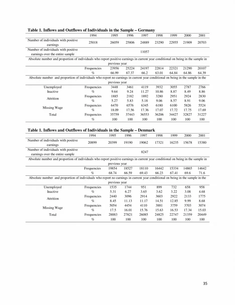
35

Table 1. Inflows and Outflows of Individuals in the Sample – Germany

1994 1995 1996 1997 1998 1999 2000 2001

Number of individuals with positive

earnings 25018 26059 25806 24889 23290 22955 21909 20703

Number of individuals with positive

earnings over the entire sample 11057

Absolute number and proportion of individuals who report positive earnings in current year conditional on being in the sample in

previous year

Frequencies 23956 25224 24197 22814 22321 21290 20107

% 66.99 67.37 66.2 63.01 64.84 64.86 64.39

Absolute number and proportion of individuals who report no earnings in current year conditional on being in the sample in the

previous year

Unemployed

Inactive

Frequencies 3448 3461 4119 3932 3055 2787 2766

% 9.64 9.24 11.27 10.86 8.87 8.49 8.86

Attrition Frequencies 1885 2182 1892 3280 2951 2924 2830

% 5.27 5.83 5.18 9.06 8.57 8.91 9.06

Missing Wage Frequencies 6470 6576 6345 6180 6100 5826 5524

% 18.09 17.56 17.36 17.07 17.72 17.75 17.69

Total

Frequencies 35759 37443 36553 36206 34427 32827 31227

% 100 100 100 100 100 100 100

Table 1. Inflows and Outflows of Individuals in the Sample – Denmark

1994 1995 1996 1997 1998 1999 2000 2001

Number of individuals with positive

earnings 20899 20399 19190 19062 17321 16235 15678 15380

Number of individuals with positive

earnings over the entire sample 8247

Absolute number and proportion of individuals who report positive earnings in current year conditional on being in the sample in

previous year

Frequencies 19854 18527 18110 16442 15334 14865 14642

% 68.74 66.59 69.43 66.23 67.41 69.6 71.6

Absolute number and proportion of individuals who report no earnings in current year conditional on being in the sample in the

previous year

Unemployed

Inactive

Frequencies 1535 1744 951 899 732 658 958

% 5.31 6.27 3.65 3.62 3.22 3.08 4.68

Attrition Frequencies 2440 3096 2914 3603 2922 2133 1775

% 8.45 11.13 11.17 14.51 12.85 9.99 8.68

Missing Wage Frequencies 5054 4454 4110 3881 3759 3703 3074

% 17.5 16.01 15.76 15.63 16.53 17.34 15.03

Total

Frequencies 28883 27821 26085 24825 22747 21359 20449

% 100 100 100 100 100 100 100

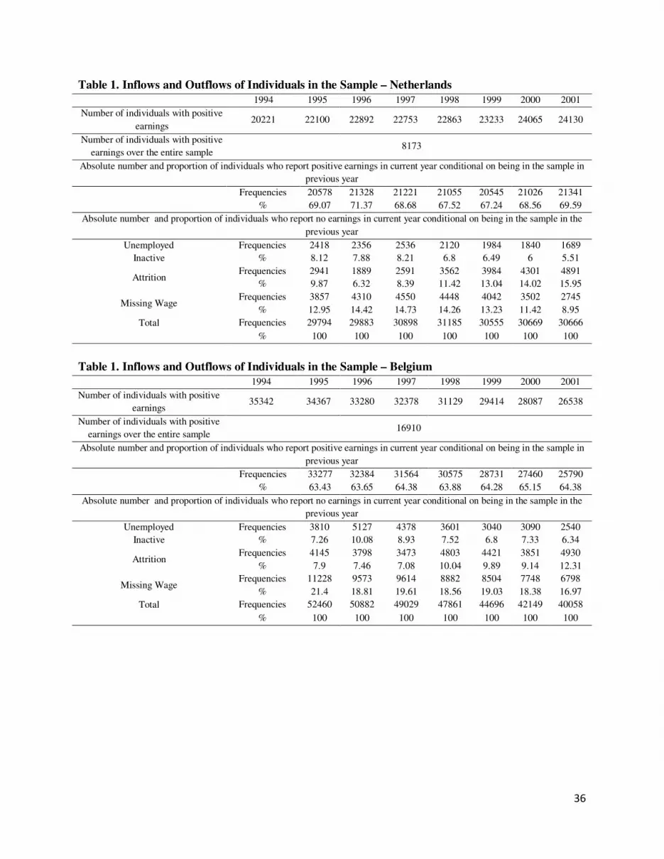
36

Table 1. Inflows and Outflows of Individuals in the Sample – Netherlands

1994 1995 1996 1997 1998 1999 2000 2001

Number of individuals with positive

earnings 20221 22100 22892 22753 22863 23233 24065 24130

Number of individuals with positive

earnings over the entire sample 8173

Absolute number and proportion of individuals who report positive earnings in current year conditional on being in the sample in

previous year

Frequencies 20578 21328 21221 21055 20545 21026 21341

% 69.07 71.37 68.68 67.52 67.24 68.56 69.59

Absolute number and proportion of individuals who report no earnings in current year conditional on being in the sample in the

previous year

Unemployed

Inactive

Frequencies 2418 2356 2536 2120 1984 1840 1689

% 8.12 7.88 8.21 6.8 6.49 6 5.51

Attrition Frequencies 2941 1889 2591 3562 3984 4301 4891

% 9.87 6.32 8.39 11.42 13.04 14.02 15.95

Missing Wage Frequencies 3857 4310 4550 4448 4042 3502 2745

% 12.95 14.42 14.73 14.26 13.23 11.42 8.95

Total

Frequencies 29794 29883 30898 31185 30555 30669 30666

% 100 100 100 100 100 100 100

Table 1. Inflows and Outflows of Individuals in the Sample – Belgium

1994 1995 1996 1997 1998 1999 2000 2001

Number of individuals with positive

earnings 35342 34367 33280 32378 31129 29414 28087 26538

Number of individuals with positive

earnings over the entire sample 16910

Absolute number and proportion of individuals who report positive earnings in current year conditional on being in the sample in

previous year

Frequencies 33277 32384 31564 30575 28731 27460 25790

% 63.43 63.65 64.38 63.88 64.28 65.15 64.38

Absolute number and proportion of individuals who report no earnings in current year conditional on being in the sample in the

previous year

Unemployed

Inactive

Frequencies 3810 5127 4378 3601 3040 3090 2540

% 7.26 10.08 8.93 7.52 6.8 7.33 6.34

Attrition Frequencies 4145 3798 3473 4803 4421 3851 4930

% 7.9 7.46 7.08 10.04 9.89 9.14 12.31

Missing Wage Frequencies 11228 9573 9614 8882 8504 7748 6798

% 21.4 18.81 19.61 18.56 19.03 18.38 16.97

Total

Frequencies 52460 50882 49029 47861 44696 42149 40058

% 100 100 100 100 100 100 100

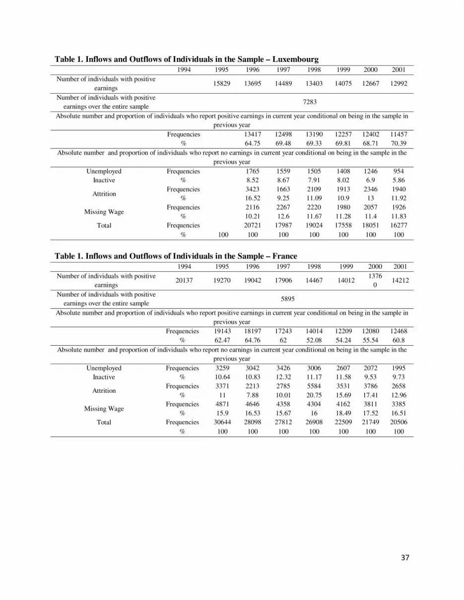
37

Table 1. Inflows and Outflows of Individuals in the Sample – Luxembourg

1994 1995 1996 1997 1998 1999 2000 2001

Number of individuals with positive

earnings 15829 13695 14489 13403 14075 12667 12992

Number of individuals with positive

earnings over the entire sample 7283

Absolute number and proportion of individuals who report positive earnings in current year conditional on being in the sample in

previous year

Frequencies

13417 12498 13190 12257 12402 11457

%

64.75 69.48 69.33 69.81 68.71 70.39

Absolute number and proportion of individuals who report no earnings in current year conditional on being in the sample in the

previous year

Unemployed

Inactive

Frequencies

1765 1559 1505 1408 1246 954

%

8.52 8.67 7.91 8.02 6.9 5.86

Attrition Frequencies

3423 1663 2109 1913 2346 1940

%

16.52 9.25 11.09 10.9 13 11.92

Missing Wage Frequencies

2116 2267 2220 1980 2057 1926

%

10.21 12.6 11.67 11.28 11.4 11.83

Total

Frequencies

20721 17987 19024 17558 18051 16277

% 100 100 100 100 100 100 100

Table 1. Inflows and Outflows of Individuals in the Sample – France

1994 1995 1996 1997 1998 1999 2000 2001

Number of individuals with positive

earnings 20137 19270 19042 17906 14467 14012

1376

0 14212

Number of individuals with positive

earnings over the entire sample 5895

Absolute number and proportion of individuals who report positive earnings in current year conditional on being in the sample in

previous year

Frequencies 19143 18197 17243 14014 12209 12080 12468

% 62.47 64.76 62 52.08 54.24 55.54 60.8

Absolute number and proportion of individuals who report no earnings in current year conditional on being in the sample in the

previous year

Unemployed

Inactive

Frequencies 3259 3042 3426 3006 2607 2072 1995

% 10.64 10.83 12.32 11.17 11.58 9.53 9.73

Attrition Frequencies 3371 2213 2785 5584 3531 3786 2658

% 11 7.88 10.01 20.75 15.69 17.41 12.96

Missing Wage Frequencies 4871 4646 4358 4304 4162 3811 3385

% 15.9 16.53 15.67 16 18.49 17.52 16.51

Total

Frequencies 30644 28098 27812 26908 22509 21749 20506

% 100 100 100 100 100 100 100

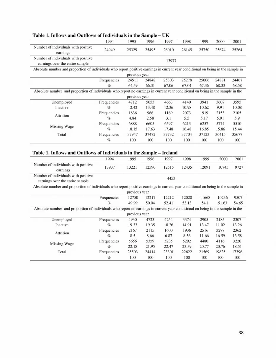
38

Table 1. Inflows and Outflows of Individuals in the Sample – UK

1994 1995 1996 1997 1998 1999 2000 2001

Number of individuals with positive

earnings 24949 25329 25495 26010 26145 25750 25674 25264

Number of individuals with positive

earnings over the entire sample 13977

Absolute number and proportion of individuals who report positive earnings in current year conditional on being in the sample in

previous year

Frequencies 24511 24848 25303 25278 25006 24881 24467

% 64.59 66.31 67.06 67.04 67.36 68.33 68.58

Absolute number and proportion of individuals who report no earnings in current year conditional on being in the sample in the

previous year

Unemployed

Inactive

Frequencies 4712 5053 4663 4140 3941 3607 3595

% 12.42 13.48 12.36 10.98 10.62 9.91 10.08

Attrition Frequencies 1836 966 1169 2073 1919 2153 2105

% 4.84 2.58 3.1 5.5 5.17 5.91 5.9

Missing Wage Frequencies 6888 6605 6597 6213 6257 5774 5510

% 18.15 17.63 17.48 16.48 16.85 15.86 15.44

Total

Frequencies 37947 37472 37732 37704 37123 36415 35677

% 100 100 100 100 100 100 100

Table 1. Inflows and Outflows of Individuals in the Sample – Ireland

1994 1995 1996 1997 1998 1999 2000 2001

Number of individuals with positive

earnings 13937 13221 12590 12515 12435 12091 10745 9727

Number of individuals with positive

earnings over the entire sample 4453

Absolute number and proportion of individuals who report positive earnings in current year conditional on being in the sample in

previous year

Frequencies 12750 12217 12212 12020 11668 10236 9507

% 49.99 50.04 52.41 53.13 54.1 51.63 54.65

Absolute number and proportion of individuals who report no earnings in current year conditional on being in the sample in the

previous year

Unemployed

Inactive

Frequencies 4930 4723 4254 3374 2905 2185 2307

% 19.33 19.35 18.26 14.91 13.47 11.02 13.26

Attrition Frequencies 2167 2115 1600 1936 2516 3288 2362

% 8.5 8.66 6.87 8.56 11.66 16.59 13.58

Missing Wage Frequencies 5656 5359 5235 5292 4480 4116 3220

% 22.18 21.95 22.47 23.39 20.77 20.76 18.51

Total

Frequencies 25503 24414 23301 22622 21569 19825 17396

% 100 100 100 100 100 100 100

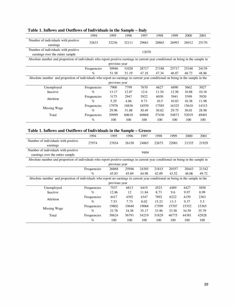
39

Table 1. Inflows and Outflows of Individuals in the Sample – Italy

1994 1995 1996 1997 1998 1999 2000 2001

Number of individuals with positive

earnings 32633 32236 32111 29661 28865 26993 26912 25170

Number of individuals with positive

earnings over the entire sample 12070

Absolute number and proportion of individuals who report positive earnings in current year conditional on being in the sample in

previous year

Frequencies 30946 31028 28717 27188 25717 25348 24139

% 51.58 51.19 47.18 47.34 46.87 48.73 48.86

Absolute number and proportion of individuals who report no earnings in current year conditional on being in the sample in the

previous year

Unemployed

Inactive

Frequencies 7900 7799 7670 6627 6890 5662 5027

% 13.17 12.87 12.6 11.54 12.56 10.88 10.18

Attrition Frequencies 3175 2947 5922 6030 5941 5399 5920

% 5.29 4.86 9.73 10.5 10.83 10.38 11.98

Missing Wage Frequencies 17978 18836 18559 17585 16325 15610 14315

% 29.96 31.08 30.49 30.62 29.75 30.01 28.98

Total

Frequencies 59999 60610 60868 57430 54873 52019 49401

% 100 100 100 100 100 100 100

Table 1. Inflows and Outflows of Individuals in the Sample – Greece

1994 1995 1996 1997 1998 1999 2000 2001

Number of individuals with positive

earnings 27974 27654 26150 24865 22675 22001 21335 21929

Number of individuals with positive

earnings over the entire sample 9404

Absolute number and proportion of individuals who report positive earnings in current year conditional on being in the sample in

previous year

Frequencies 26868 25946 24385 21815 20357 20443 21342

% 45.83 45.69 44.98 42.09 43.52 46.06 49.72

Absolute number and proportion of individuals who report no earnings in current year conditional on being in the sample in the

previous year

Unemployed

Inactive

Frequencies 7537 6813 6419 4523 4489 4427 3858

% 12.86 12 11.84 8.73 9.6 9.97 8.99

Attrition Frequencies 4417 4392 4347 7892 6222 4159 2363

% 7.53 7.73 8.02 15.23 13.3 9.37 5.5

Missing Wage Frequencies 19802 19640 19068 17599 15707 15352 15365

% 33.78 34.58 35.17 33.96 33.58 34.59 35.79

Total

Frequencies 58624 56791 54219 51829 46775 44381 42928

% 100 100 100 100 100 100 100

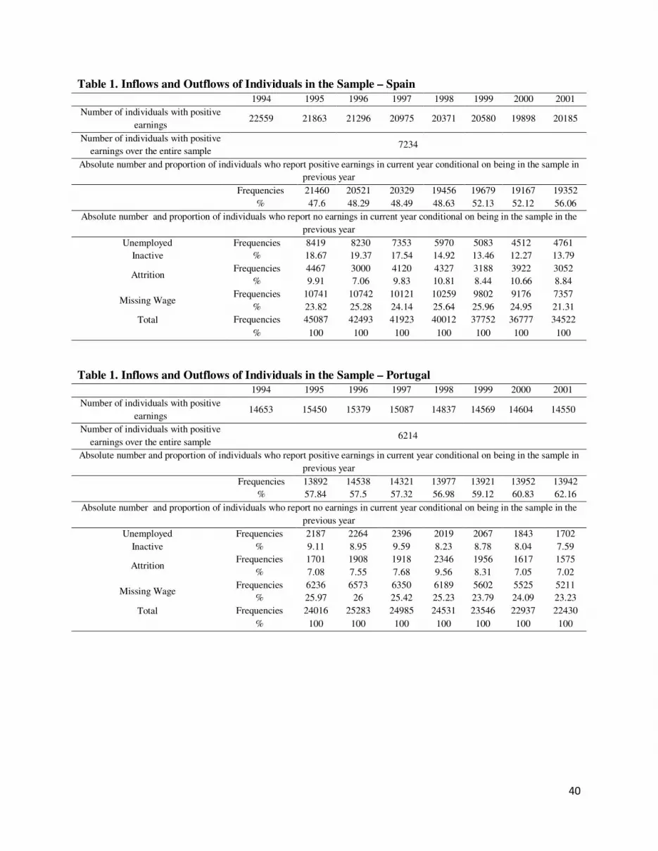
40

Table 1. Inflows and Outflows of Individuals in the Sample – Spain

1994 1995 1996 1997 1998 1999 2000 2001

Number of individuals with positive

earnings 22559 21863 21296 20975 20371 20580 19898 20185

Number of individuals with positive

earnings over the entire sample 7234

Absolute number and proportion of individuals who report positive earnings in current year conditional on being in the sample in

previous year

Frequencies 21460 20521 20329 19456 19679 19167 19352

% 47.6 48.29 48.49 48.63 52.13 52.12 56.06

Absolute number and proportion of individuals who report no earnings in current year conditional on being in the sample in the

previous year

Unemployed

Inactive

Frequencies 8419 8230 7353 5970 5083 4512 4761

% 18.67 19.37 17.54 14.92 13.46 12.27 13.79

Attrition Frequencies 4467 3000 4120 4327 3188 3922 3052

% 9.91 7.06 9.83 10.81 8.44 10.66 8.84

Missing Wage Frequencies 10741 10742 10121 10259 9802 9176 7357

% 23.82 25.28 24.14 25.64 25.96 24.95 21.31

Total

Frequencies 45087 42493 41923 40012 37752 36777 34522

% 100 100 100 100 100 100 100

Table 1. Inflows and Outflows of Individuals in the Sample – Portugal

1994 1995 1996 1997 1998 1999 2000 2001

Number of individuals with positive

earnings 14653 15450 15379 15087 14837 14569 14604 14550

Number of individuals with positive

earnings over the entire sample 6214

Absolute number and proportion of individuals who report positive earnings in current year conditional on being in the sample in

previous year

Frequencies 13892 14538 14321 13977 13921 13952 13942

% 57.84 57.5 57.32 56.98 59.12 60.83 62.16

Absolute number and proportion of individuals who report no earnings in current year conditional on being in the sample in the

previous year

Unemployed

Inactive

Frequencies 2187 2264 2396 2019 2067 1843 1702

% 9.11 8.95 9.59 8.23 8.78 8.04 7.59

Attrition Frequencies 1701 1908 1918 2346 1956 1617 1575

% 7.08 7.55 7.68 9.56 8.31 7.05 7.02

Missing Wage Frequencies 6236 6573 6350 6189 5602 5525 5211

% 25.97 26 25.42 25.23 23.79 24.09 23.23

Total

Frequencies 24016 25283 24985 24531 23546 22937 22430

% 100 100 100 100 100 100 100

41

Table 1. Inflows and Outflows of Individuals in the Sample – Austria

1994 1995 1996 1997 1998 1999 2000 2001

Number of individuals with positive

earnings 17944 17789 17199 16209 15162 13816 13056

Number of individuals with positive

earnings over the entire sample 8127

Absolute number and proportion of individuals who report positive earnings in current year conditional on being in the sample in

previous year

Frequencies 16472 16384 15634 14551 13403 12601

% 67.96 68.2 67.49 67.2 66.51 68.21

Absolute number and proportion of individuals who report no earnings in current year conditional on being in the sample in the

previous year

Unemployed

Inactive

Frequencies 1209 1231 906 790 803 843

% 4.99 5.12 3.91 3.65 3.98 4.56

Attrition Frequencies 2195 2080 2435 2470 2409 1794

% 9.06 8.66 10.51 11.41 11.95 9.71

Missing Wage Frequencies 4361 4330 4189 3842 3538 3235

% 17.99 18.02 18.08 17.74 17.56 17.51

Total

Frequencies 24237 24025 23164 21653 20153 18473

%

100 100 100 100 100 100

Table 1. Inflows and Outflows of Individuals in the Sample – Finland

1996 1997 1998 1999 2000 2001

Number of individuals with positive

earnings

15811 15845 15895 15546 13329 13057

Number of individuals with positive

earnings over the entire sample 6913

Absolute number and proportion of individuals who report positive earnings in current year conditional on being in the sample in

previous year

Frequencies

15246 15345 14753 12756 12588

%

55.95 57.2 59.29 53.83 64.16

Absolute number and proportion of individuals who report no earnings in current year conditional on being in the sample in the

previous year

Unemployed

Inactive

Frequencies

3446 2327 1657 1326 1267

%

12.65 8.67 6.66 5.6 6.46

Attrition Frequencies

1933 3219 2658 5219 1708

%

7.09 12 10.68 22.02 8.71

Missing Wage Frequencies

6623 5937 5814 4398 4057

%

24.31 22.13 23.37 18.56 20.68

Total

Frequencies

27248 26828 24882 23699 19620

%

100 100 100 100 100

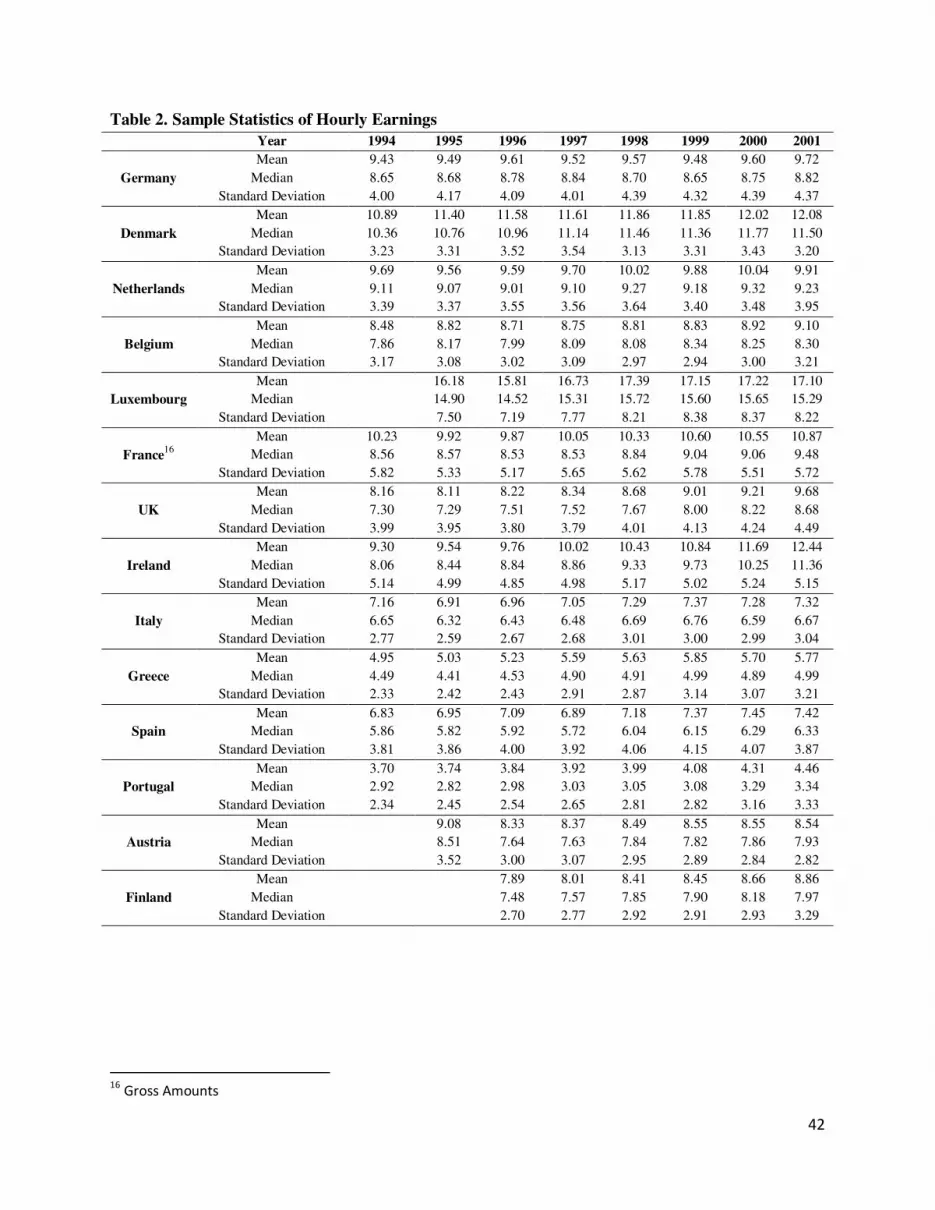
42

Table 2. Sample Statistics of Hourly Earnings

Year 1994 1995 1996 1997 1998 1999 2000 2001

Germany

Mean 9.43 9.49 9.61 9.52 9.57 9.48 9.60 9.72

Median 8.65 8.68 8.78 8.84 8.70 8.65 8.75 8.82

Standard Deviation 4.00 4.17 4.09 4.01 4.39 4.32 4.39 4.37

Denmark

Mean 10.89 11.40 11.58 11.61 11.86 11.85 12.02 12.08

Median 10.36 10.76 10.96 11.14 11.46 11.36 11.77 11.50

Standard Deviation 3.23 3.31 3.52 3.54 3.13 3.31 3.43 3.20

Netherlands

Mean 9.69 9.56 9.59 9.70 10.02 9.88 10.04 9.91

Median 9.11 9.07 9.01 9.10 9.27 9.18 9.32 9.23

Standard Deviation 3.39 3.37 3.55 3.56 3.64 3.40 3.48 3.95

Belgium

Mean 8.48 8.82 8.71 8.75 8.81 8.83 8.92 9.10

Median 7.86 8.17 7.99 8.09 8.08 8.34 8.25 8.30

Standard Deviation 3.17 3.08 3.02 3.09 2.97 2.94 3.00 3.21

Luxembourg

Mean 16.18 15.81 16.73 17.39 17.15 17.22 17.10

Median 14.90 14.52 15.31 15.72 15.60 15.65 15.29

Standard Deviation 7.50 7.19 7.77 8.21 8.38 8.37 8.22

France16

Mean 10.23 9.92 9.87 10.05 10.33 10.60 10.55 10.87

Median 8.56 8.57 8.53 8.53 8.84 9.04 9.06 9.48

Standard Deviation 5.82 5.33 5.17 5.65 5.62 5.78 5.51 5.72

UK

Mean 8.16 8.11 8.22 8.34 8.68 9.01 9.21 9.68

Median 7.30 7.29 7.51 7.52 7.67 8.00 8.22 8.68

Standard Deviation 3.99 3.95 3.80 3.79 4.01 4.13 4.24 4.49

Ireland

Mean 9.30 9.54 9.76 10.02 10.43 10.84 11.69 12.44

Median 8.06 8.44 8.84 8.86 9.33 9.73 10.25 11.36

Standard Deviation 5.14 4.99 4.85 4.98 5.17 5.02 5.24 5.15

Italy

Mean 7.16 6.91 6.96 7.05 7.29 7.37 7.28 7.32

Median 6.65 6.32 6.43 6.48 6.69 6.76 6.59 6.67

Standard Deviation 2.77 2.59 2.67 2.68 3.01 3.00 2.99 3.04

Greece

Mean 4.95 5.03 5.23 5.59 5.63 5.85 5.70 5.77

Median 4.49 4.41 4.53 4.90 4.91 4.99 4.89 4.99

Standard Deviation 2.33 2.42 2.43 2.91 2.87 3.14 3.07 3.21

Spain

Mean 6.83 6.95 7.09 6.89 7.18 7.37 7.45 7.42

Median 5.86 5.82 5.92 5.72 6.04 6.15 6.29 6.33

Standard Deviation 3.81 3.86 4.00 3.92 4.06 4.15 4.07 3.87

Portugal

Mean 3.70 3.74 3.84 3.92 3.99 4.08 4.31 4.46

Median 2.92 2.82 2.98 3.03 3.05 3.08 3.29 3.34

Standard Deviation 2.34 2.45 2.54 2.65 2.81 2.82 3.16 3.33

Austria

Mean 9.08 8.33 8.37 8.49 8.55 8.55 8.54

Median 8.51 7.64 7.63 7.84 7.82 7.86 7.93

Standard Deviation 3.52 3.00 3.07 2.95 2.89 2.84 2.82

Finland

Mean 7.89 8.01 8.41 8.45 8.66 8.86

Median 7.48 7.57 7.85 7.90 8.18 7.97

Standard Deviation 2.70 2.77 2.92 2.91 2.93 3.29

16

Gross Amounts

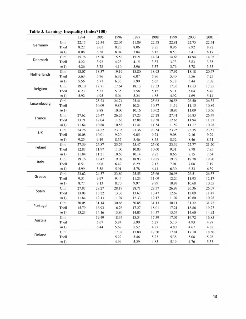
43

Table 3. Earnings Inequality (Index*100)

1994 1995 1996 1997 1998 1999 2000 2001

Germany Gini 22.15 22.34 22.04 21.89 22.58 22.81 22.75 22.54

Theil 8.22 8.61 8.23 8.06 8.85 8.96 8.92 8.72

A(1) 8.08 8.38 8.04 7.84 8.12 8.53 8.41 8.17

Denmark Gini 15.76 15.26 15.52 15.21 14.24 14.68 14.94 14.05

Theil 4.22 3.92 4.23 4.15 3.37 3.73 3.83 3.35

A(1) 4.26 3.78 4.10 3.96 3.37 3.76 3.78 3.33

Netherlands Gini 18.07 18.37 19.19 18.80 18.93 17.92 18.18 20.67

Theil 5.63 5.76 6.32 6.07 5.96 5.40 5.56 7.25

A(1) 5.56 5.77 6.33 5.90 5.65 5.18 5.44 7.08

Belgium Gini 19.10 17.71 17.64 18.13 17.53 17.33 17.13 17.85

Theil 6.23 5.37 5.35 5.58 5.15 5.11 5.04 5.48

A(1) 5.92 4.95 5.04 5.24 4.85 4.92 4.69 5.14

Luxembourg Gini 25.23 24.74 25.41 25.62 26.58 26.50 26.32

Theil 10.09 9.85 10.24 10.37 11.19 11.15 10.89

A(1) 9.88 10.00 10.16 10.02 10.95 11.09 10.66

France Gini 27.62 26.47 26.26 27.23 27.28 27.41 26.83 26.49

Theil 13.21 12.04 11.63 12.88 12.58 12.65 11.94 11.87

A(1) 11.64 10.88 10.58 11.41 11.54 11.59 11.17 10.98

UK Gini 24.26 24.22 23.35 23.36 23.54 23.25 23.35 23.51

Theil 10.08 10.01 9.20 9.05 9.24 9.08 9.16 9.29

A(1) 9.25 9.19 8.57 8.46 8.55 8.32 8.46 8.51

Ireland Gini 27.59 26.87 25.76 25.47 25.00 23.39 22.77 21.70

Theil 12.87 11.97 11.00 10.83 10.60 9.31 8.78 7.85

A(1) 11.84 11.21 10.50 10.14 9.85 8.66 8.15 7.64

Italy Gini 19.16 18.47 19.02 18.93 19.85 19.72 19.78 19.90

Theil 6.51 6.08 6.42 6.29 7.13 7.01 7.08 7.19

A(1) 5.99 5.58 5.91 5.78 6.41 6.30 6.33 6.39

Greece Gini 23.62 24.37 23.80 25.55 25.66 26.98 26.51 26.37

Theil 9.51 9.97 9.44 11.23 11.09 12.20 11.93 12.17

A(1) 8.77 9.13 8.70 9.97 9.99 10.97 10.68 10.55

Spain Gini 27.87 28.27 28.19 28.71 28.37 26.99 26.36 26.07

Theil 13.08 13.22 13.36 13.67 13.47 12.69 12.09 11.47

A(1) 11.84 12.13 11.94 12.33 12.17 11.07 10.60 10.28

Portugal Gini 30.05 31.14 30.66 30.85 31.13 30.11 31.32 31.72

Theil 15.79 16.93 16.76 17.27 18.01 17.21 18.86 19.27

A(1) 13.23 14.16 13.80 14.05 14.37 13.55 14.60 14.92

Austria Gini 19.49 18.34 18.34 17.39 17.07 16.72 16.85

Theil 6.67 5.84 5.90 5.27 5.10 4.93 4.97

A(1) 6.44 5.62 5.52 4.87 4.80 4.67 4.82

Finland Gini 17.32 17.80 17.30 17.81 17.10 18.50

Theil 5.22 5.46 5.23 5.38 5.08 5.98

A(1) 4.94 5.29 4.83 5.19 4.76 5.53

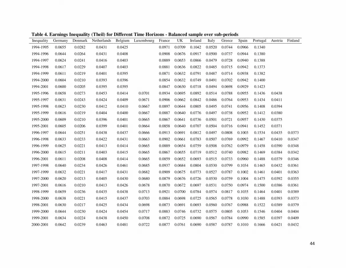
44

Table 4. Earnings Inequality (Theil) for Different Time Horizons - Balanced sample over sub-periods

Inequality Germany Denmark Netherlands Belgium Luxembourg France UK Ireland Italy Greece Spain Portugal Austria Finland

1994-1995 0.0655 0.0282 0.0431 0.0425 0.0971 0.0709 0.1042 0.0520 0.0744 0.0966 0.1340

1994-1996 0.0644 0.0264 0.0431 0.0408 0.0908 0.0676 0.0917 0.0500 0.0737 0.0944 0.1380

1994-1997 0.0624 0.0241 0.0416 0.0403 0.0889 0.0653 0.0866 0.0479 0.0728 0.0940 0.1388

1994-1998 0.0617 0.0229 0.0407 0.0403 0.0881 0.0636 0.0822 0.0485 0.0715 0.0942 0.1373

1994-1999 0.0611 0.0219 0.0401 0.0395 0.0871 0.0632 0.0791 0.0487 0.0714 0.0938 0.1382

1994-2000 0.0604 0.0210 0.0393 0.0396 0.0854 0.0632 0.0749 0.0491 0.0702 0.0942 0.1400

1994-2001 0.0600 0.0205 0.0395 0.0395 0.0847 0.0630 0.0718 0.0494 0.0698 0.0929 0.1423

1995-1996 0.0658 0.0273 0.0453 0.0414 0.0701 0.0934 0.0695 0.0892 0.0514 0.0788 0.0955 0.1436 0.0438

1995-1997 0.0631 0.0243 0.0424 0.0409 0.0671 0.0906 0.0662 0.0842 0.0486 0.0764 0.0953 0.1434 0.0411

1995-1998 0.0623 0.0230 0.0412 0.0410 0.0667 0.0897 0.0644 0.0805 0.0495 0.0741 0.0956 0.1408 0.0394

1995-1999 0.0616 0.0219 0.0404 0.0400 0.0667 0.0887 0.0640 0.0776 0.0497 0.0738 0.0952 0.1412 0.0380

1995-2000 0.0609 0.0210 0.0396 0.0401 0.0665 0.0867 0.0641 0.0736 0.0501 0.0721 0.0957 0.1430 0.0375

1995-2001 0.0605 0.0206 0.0399 0.0401 0.0664 0.0858 0.0640 0.0707 0.0504 0.0716 0.0941 0.1452 0.0371

1996-1997 0.0644 0.0251 0.0438 0.0437 0.0666 0.0913 0.0691 0.0812 0.0497 0.0808 0.1003 0.1534 0.0435 0.0373

1996-1998 0.0633 0.0233 0.0422 0.0431 0.0663 0.0902 0.0661 0.0783 0.0507 0.0769 0.0992 0.1467 0.0410 0.0347

1996-1999 0.0625 0.0221 0.0413 0.0414 0.0665 0.0889 0.0654 0.0759 0.0508 0.0762 0.0979 0.1458 0.0390 0.0348

1996-2000 0.0615 0.0211 0.0403 0.0415 0.0665 0.0867 0.0655 0.0719 0.0512 0.0740 0.0982 0.1469 0.0384 0.0342

1996-2001 0.0611 0.0208 0.0408 0.0414 0.0665 0.0859 0.0652 0.0693 0.0515 0.0733 0.0960 0.1488 0.0379 0.0346

1997-1998 0.0640 0.0234 0.0426 0.0461 0.0685 0.0937 0.0684 0.0804 0.0530 0.0799 0.1034 0.1465 0.0432 0.0361

1997-1999 0.0632 0.0221 0.0417 0.0431 0.0682 0.0909 0.0675 0.0773 0.0527 0.0787 0.1002 0.1461 0.0401 0.0363

1997-2000 0.0620 0.0213 0.0405 0.0430 0.0680 0.0879 0.0676 0.0726 0.0530 0.0759 0.1004 0.1475 0.0392 0.0355

1997-2001 0.0616 0.0210 0.0413 0.0426 0.0678 0.0870 0.0672 0.0697 0.0531 0.0750 0.0974 0.1500 0.0386 0.0361

1998-1999 0.0659 0.0236 0.0435 0.0438 0.0713 0.0921 0.0700 0.0784 0.0574 0.0817 0.1035 0.1464 0.0401 0.0389

1998-2000 0.0638 0.0221 0.0415 0.0437 0.0703 0.0884 0.0698 0.0725 0.0565 0.0778 0.1030 0.1488 0.0393 0.0373

1998-2001 0.0630 0.0217 0.0425 0.0434 0.0698 0.0873 0.0691 0.0693 0.0560 0.0767 0.0988 0.1522 0.0389 0.0379

1999-2000 0.0644 0.0230 0.0424 0.0454 0.0717 0.0883 0.0746 0.0732 0.0575 0.0805 0.1053 0.1546 0.0404 0.0404

1999-2001 0.0634 0.0224 0.0438 0.0450 0.0708 0.0872 0.0725 0.0690 0.0567 0.0784 0.0990 0.1585 0.0397 0.0409

2000-2001 0.0642 0.0239 0.0463 0.0481 0.0722 0.0877 0.0761 0.0690 0.0587 0.0787 0.1010 0.1666 0.0421 0.0432

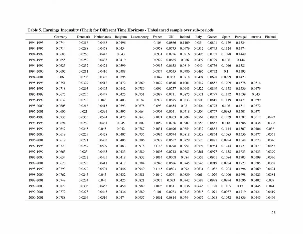
45

Table 5. Earnings Inequality (Theil) for Different Time Horizons - Unbalanced sample over sub-periods

Germany Denmark Netherlands Belgium Luxembourg France UK Ireland Italy Greece Spain Portugal Austria Finland

1994-1995 0.0744 0.0316 0.0468 0.0496 0.106 0.0866 0.1109 0.054 0.0801 0.1179 0.1524

1994-1996 0.0714 0.0288 0.0458 0.0454 0.0958 0.0775 0.0979 0.0512 0.0745 0.1124 0.1474

1994-1997 0.0688 0.0266 0.0443 0.043 0.0931 0.0726 0.0916 0.0495 0.0767 0.1078 0.1449

1994-1998 0.0655 0.0252 0.0435 0.0419 0.0929 0.0685 0.086 0.0497 0.0729 0.106 0.144

1994-1999 0.0623 0.0232 0.0424 0.0399 0.0915 0.0653 0.0819 0.049 0.0756 0.1046 0.1381

1994-2000 0.0602 0.0211 0.0416 0.0388 0.0874 0.0635 0.0786 0.0496 0.0732 0.1 0.1393

1994-2001 0.06 0.0205 0.0395 0.0395 0.0847 0.063 0.0718 0.0494 0.0698 0.0929 0.1423

1995-1996 0.0751 0.0329 0.0512 0.0472 0.0869 0.1029 0.0816 0.1001 0.0547 0.0852 0.1209 0.1578 0.0514

1995-1997 0.0718 0.0293 0.0465 0.0442 0.0786 0.099 0.0757 0.0943 0.0522 0.0849 0.1158 0.1536 0.0479

1995-1998 0.0675 0.0275 0.0449 0.0425 0.0751 0.0989 0.0711 0.0875 0.0521 0.0797 0.1132 0.1539 0.043

1995-1999 0.0632 0.0238 0.043 0.0403 0.074 0.0972 0.0675 0.0833 0.0503 0.0815 0.1119 0.1471 0.0399

1995-2000 0.0605 0.0218 0.0415 0.0393 0.0678 0.093 0.0654 0.081 0.0504 0.0795 0.106 0.1511 0.0372

1995-2001 0.0606 0.021 0.0391 0.0395 0.0664 0.0903 0.0641 0.0718 0.0504 0.0767 0.0985 0.1501 0.0371

1996-1997 0.0735 0.0353 0.0524 0.0475 0.0843 0.1071 0.0803 0.0994 0.0564 0.0933 0.1239 0.1582 0.0512 0.0422

1996-1998 0.0694 0.0282 0.0481 0.045 0.0802 0.1059 0.0736 0.0907 0.0556 0.0857 0.118 0.1586 0.0438 0.0398

1996-1999 0.0647 0.0245 0.045 0.042 0.0787 0.1031 0.0696 0.0854 0.0532 0.0882 0.1144 0.1507 0.0406 0.036

1996-2000 0.0619 0.0229 0.0428 0.0407 0.0735 0.0985 0.0674 0.0818 0.0528 0.0854 0.1085 0.1556 0.0377 0.0351

1996-2001 0.0619 0.0221 0.0403 0.0405 0.0706 0.0927 0.0657 0.0729 0.0523 0.0821 0.0994 0.1548 0.0373 0.0346

1997-1998 0.0723 0.0289 0.0509 0.0483 0.0918 0.1148 0.0798 0.0951 0.0594 0.0964 0.1244 0.1727 0.0477 0.0453

1997-1999 0.0663 0.025 0.0463 0.0433 0.0889 0.1093 0.0742 0.0881 0.0561 0.0977 0.1158 0.1633 0.0433 0.0399

1997-2000 0.0634 0.0232 0.0435 0.0418 0.0832 0.1014 0.0708 0.084 0.0557 0.0951 0.1084 0.1703 0.0399 0.0376

1997-2001 0.0628 0.0223 0.0411 0.0417 0.0784 0.0943 0.0686 0.0745 0.0546 0.0919 0.0984 0.1723 0.0385 0.0368

1998-1999 0.0793 0.0272 0.0501 0.0446 0.0949 0.1145 0.0803 0.092 0.0631 0.1082 0.1204 0.1696 0.0469 0.0424

1998-2000 0.0762 0.0245 0.045 0.0432 0.0881 0.1049 0.0761 0.0839 0.061 0.1029 0.1096 0.1698 0.0423 0.0384

1998-2001 0.0749 0.0234 0.043 0.0425 0.0821 0.0973 0.073 0.0742 0.0587 0.0998 0.0994 0.1696 0.0402 0.037

1999-2000 0.0827 0.0305 0.0453 0.0458 0.0989 0.1095 0.0811 0.0836 0.0645 0.1128 0.1105 0.171 0.0445 0.044

1999-2001 0.0772 0.0273 0.0443 0.0436 0.0889 0.101 0.0763 0.0735 0.0618 0.1071 0.0987 0.1719 0.0421 0.0419

2000-2001 0.0788 0.0294 0.0516 0.0474 0.0957 0.1061 0.0814 0.0744 0.0657 0.1098 0.1032 0.1836 0.0445 0.0466

46

Table 6. Shorrocks Mobility based on Theil for Different Time Horizons - Balanced sample over sub-periods

shor bal Germany Denmark Netherlands Belgium Luxembourg France UK Ireland Italy Greece Spain Portugal Austria Finland

1994-1995 0.0539 0.0994 0.0807 0.1044 0.0989 0.0919 0.0588 0.0741 0.1125 0.0698 0.0496

1994-1996 0.0749 0.1588 0.1002 0.1325 0.1260 0.1332 0.1054 0.1027 0.1285 0.0964 0.0689

1994-1997 0.0912 0.1922 0.1161 0.1543 0.1328 0.1471 0.1178 0.1240 0.1489 0.1096 0.0769

1994-1998 0.1021 0.2152 0.1316 0.1576 0.1313 0.1637 0.1335 0.1358 0.1601 0.1173 0.0816

1994-1999 0.1115 0.2333 0.1460 0.1698 0.1305 0.1688 0.1475 0.1418 0.1664 0.1221 0.0795

1994-2000 0.1170 0.2555 0.1580 0.1772 0.1343 0.1799 0.1655 0.1451 0.1745 0.1286 0.0800

1994-2001 0.1240 0.2670 0.1729 0.1850 0.1348 0.1857 0.1757 0.1489 0.1803 0.1321 0.0932

1995-1996 0.0451 0.1123 0.0557 0.0789 0.0581 0.0676 0.0955 0.0728 0.0635 0.0670 0.0662 0.0515 0.1159

1995-1997 0.0723 0.1592 0.0925 0.1195 0.0874 0.0895 0.1215 0.0924 0.0966 0.1088 0.0869 0.0632 0.1690

1995-1998 0.0866 0.1893 0.1157 0.1283 0.0922 0.0923 0.1409 0.1082 0.1140 0.1299 0.0991 0.0696 0.1793

1995-1999 0.0983 0.2111 0.1343 0.1461 0.0948 0.0949 0.1497 0.1259 0.1225 0.1408 0.1061 0.0687 0.1894

1995-2000 0.1051 0.2368 0.1484 0.1563 0.0992 0.1026 0.1631 0.1461 0.1273 0.1521 0.1139 0.0700 0.1932

1995-2001 0.1129 0.2479 0.1642 0.1657 0.1036 0.1060 0.1689 0.1574 0.1326 0.1598 0.1188 0.0853 0.1979

1996-1997 0.0540 0.1169 0.0724 0.0867 0.0563 0.0608 0.0811 0.0642 0.0662 0.0715 0.0644 0.0339 0.1151 0.1004

1996-1998 0.0744 0.1634 0.0994 0.1049 0.0727 0.0715 0.1155 0.0854 0.0952 0.1045 0.0855 0.0508 0.1348 0.1501

1996-1999 0.0882 0.1900 0.1206 0.1308 0.0796 0.0792 0.1301 0.1083 0.1078 0.1192 0.0957 0.0536 0.1528 0.1728

1996-2000 0.0962 0.2200 0.1360 0.1419 0.0863 0.0891 0.1471 0.1321 0.1141 0.1331 0.1049 0.0585 0.1602 0.1886

1996-2001 0.1046 0.2305 0.1526 0.1520 0.0918 0.0935 0.1546 0.1441 0.1207 0.1420 0.1115 0.0774 0.1682 0.2184

1997-1998 0.0528 0.1019 0.0597 0.0605 0.0570 0.0405 0.0662 0.0525 0.0659 0.0695 0.0585 0.0312 0.0730 0.1031

1997-1999 0.0709 0.1424 0.0914 0.1047 0.0689 0.0595 0.0926 0.0845 0.0850 0.0920 0.0810 0.0375 0.1110 0.1366

1997-2000 0.0821 0.1816 0.1151 0.1207 0.0766 0.0738 0.1162 0.1128 0.0956 0.1099 0.0926 0.0471 0.1286 0.1564

1997-2001 0.0924 0.1944 0.1349 0.1338 0.0829 0.0798 0.1269 0.1271 0.1047 0.1221 0.1024 0.0702 0.1404 0.1922

1998-1999 0.0442 0.0950 0.0691 0.0779 0.0344 0.0393 0.0696 0.0613 0.0501 0.0503 0.0524 0.0216 0.0678 0.0885

1998-2000 0.0622 0.1575 0.1025 0.1030 0.0507 0.0587 0.1014 0.1001 0.0692 0.0772 0.0738 0.0359 0.0982 0.1222

1998-2001 0.0779 0.1732 0.1243 0.1172 0.0621 0.0676 0.1134 0.1171 0.0836 0.0958 0.0894 0.0629 0.1131 0.1689

1999-2000 0.0466 0.1136 0.0843 0.0672 0.0374 0.0447 0.0609 0.0762 0.0483 0.0498 0.0539 0.0221 0.0682 0.0796

1999-2001 0.0681 0.1398 0.1122 0.0891 0.0525 0.0580 0.0844 0.1033 0.0707 0.0794 0.0809 0.0522 0.0950 0.1376

2000-2001 0.0512 0.0971 0.0794 0.0550 0.0368 0.0425 0.0543 0.0679 0.0493 0.0585 0.0623 0.0419 0.0579 0.1066

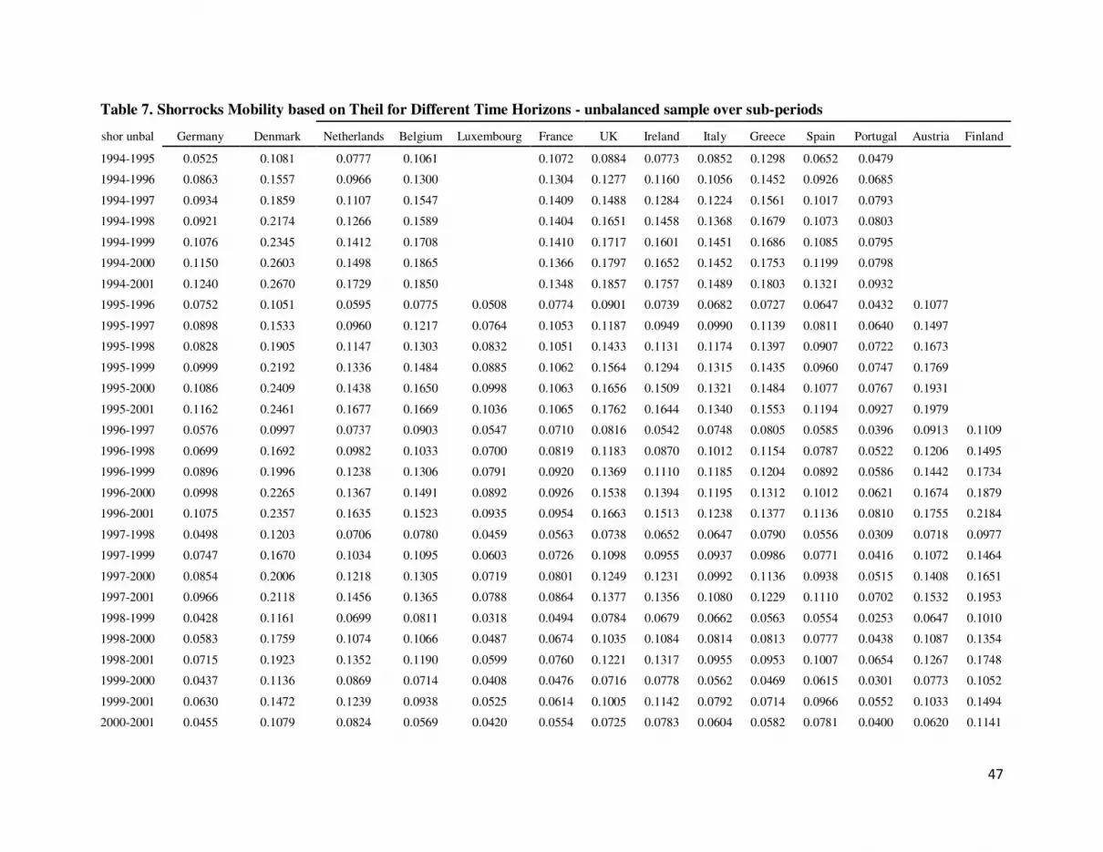
47

Table 7. Shorrocks Mobility based on Theil for Different Time Horizons - unbalanced sample over sub-periods

shor unbal Germany Denmark Netherlands Belgium Luxembourg France UK Ireland Italy Greece Spain Portugal Austria Finland

1994-1995 0.0525 0.1081 0.0777 0.1061 0.1072 0.0884 0.0773 0.0852 0.1298 0.0652 0.0479

1994-1996 0.0863 0.1557 0.0966 0.1300 0.1304 0.1277 0.1160 0.1056 0.1452 0.0926 0.0685

1994-1997 0.0934 0.1859 0.1107 0.1547 0.1409 0.1488 0.1284 0.1224 0.1561 0.1017 0.0793

1994-1998 0.0921 0.2174 0.1266 0.1589 0.1404 0.1651 0.1458 0.1368 0.1679 0.1073 0.0803

1994-1999 0.1076 0.2345 0.1412 0.1708 0.1410 0.1717 0.1601 0.1451 0.1686 0.1085 0.0795

1994-2000 0.1150 0.2603 0.1498 0.1865 0.1366 0.1797 0.1652 0.1452 0.1753 0.1199 0.0798

1994-2001 0.1240 0.2670 0.1729 0.1850 0.1348 0.1857 0.1757 0.1489 0.1803 0.1321 0.0932

1995-1996 0.0752 0.1051 0.0595 0.0775 0.0508 0.0774 0.0901 0.0739 0.0682 0.0727 0.0647 0.0432 0.1077

1995-1997 0.0898 0.1533 0.0960 0.1217 0.0764 0.1053 0.1187 0.0949 0.0990 0.1139 0.0811 0.0640 0.1497

1995-1998 0.0828 0.1905 0.1147 0.1303 0.0832 0.1051 0.1433 0.1131 0.1174 0.1397 0.0907 0.0722 0.1673

1995-1999 0.0999 0.2192 0.1336 0.1484 0.0885 0.1062 0.1564 0.1294 0.1315 0.1435 0.0960 0.0747 0.1769

1995-2000 0.1086 0.2409 0.1438 0.1650 0.0998 0.1063 0.1656 0.1509 0.1321 0.1484 0.1077 0.0767 0.1931

1995-2001 0.1162 0.2461 0.1677 0.1669 0.1036 0.1065 0.1762 0.1644 0.1340 0.1553 0.1194 0.0927 0.1979

1996-1997 0.0576 0.0997 0.0737 0.0903 0.0547 0.0710 0.0816 0.0542 0.0748 0.0805 0.0585 0.0396 0.0913 0.1109

1996-1998 0.0699 0.1692 0.0982 0.1033 0.0700 0.0819 0.1183 0.0870 0.1012 0.1154 0.0787 0.0522 0.1206 0.1495

1996-1999 0.0896 0.1996 0.1238 0.1306 0.0791 0.0920 0.1369 0.1110 0.1185 0.1204 0.0892 0.0586 0.1442 0.1734

1996-2000 0.0998 0.2265 0.1367 0.1491 0.0892 0.0926 0.1538 0.1394 0.1195 0.1312 0.1012 0.0621 0.1674 0.1879

1996-2001 0.1075 0.2357 0.1635 0.1523 0.0935 0.0954 0.1663 0.1513 0.1238 0.1377 0.1136 0.0810 0.1755 0.2184

1997-1998 0.0498 0.1203 0.0706 0.0780 0.0459 0.0563 0.0738 0.0652 0.0647 0.0790 0.0556 0.0309 0.0718 0.0977

1997-1999 0.0747 0.1670 0.1034 0.1095 0.0603 0.0726 0.1098 0.0955 0.0937 0.0986 0.0771 0.0416 0.1072 0.1464

1997-2000 0.0854 0.2006 0.1218 0.1305 0.0719 0.0801 0.1249 0.1231 0.0992 0.1136 0.0938 0.0515 0.1408 0.1651

1997-2001 0.0966 0.2118 0.1456 0.1365 0.0788 0.0864 0.1377 0.1356 0.1080 0.1229 0.1110 0.0702 0.1532 0.1953

1998-1999 0.0428 0.1161 0.0699 0.0811 0.0318 0.0494 0.0784 0.0679 0.0662 0.0563 0.0554 0.0253 0.0647 0.1010

1998-2000 0.0583 0.1759 0.1074 0.1066 0.0487 0.0674 0.1035 0.1084 0.0814 0.0813 0.0777 0.0438 0.1087 0.1354

1998-2001 0.0715 0.1923 0.1352 0.1190 0.0599 0.0760 0.1221 0.1317 0.0955 0.0953 0.1007 0.0654 0.1267 0.1748

1999-2000 0.0437 0.1136 0.0869 0.0714 0.0408 0.0476 0.0716 0.0778 0.0562 0.0469 0.0615 0.0301 0.0773 0.1052

1999-2001 0.0630 0.1472 0.1239 0.0938 0.0525 0.0614 0.1005 0.1142 0.0792 0.0714 0.0966 0.0552 0.1033 0.1494

2000-2001 0.0455 0.1079 0.0824 0.0569 0.0420 0.0554 0.0725 0.0783 0.0604 0.0582 0.0781 0.0400 0.0620 0.1141

48

Table 8. Fields Mobility based on Theil for Different Time Horizons - Balanced sample over sub-periods

Fields bal Germany Denmark Netherlands Belgium Luxembourg France UK Ireland Italy Greece Spain Portugal Austria Finland

1994-1995 0.0750 0.1419 0.1012 0.1772 0.1277 0.1178 0.1042 0.0913 0.1222 0.1155 0.0524

1994-1996 0.0917 0.1964 0.1002 0.2087 0.1843 0.1585 0.2116 0.1276 0.1307 0.1354 0.0236

1994-1997 0.1191 0.2673 0.1326 0.2192 0.2017 0.1868 0.2557 0.1634 0.1415 0.1392 0.0180

1994-1998 0.1286 0.3032 0.1513 0.2185 0.2091 0.2086 0.2930 0.1534 0.1568 0.1372 0.0286

1994-1999 0.1378 0.3347 0.1642 0.2345 0.2175 0.2126 0.3200 0.1504 0.1574 0.1405 0.0225

1994-2000 0.1476 0.3607 0.1801 0.2331 0.2331 0.2129 0.3560 0.1432 0.1726 0.1367 0.0093

1994-2001 0.1533 0.3762 0.1751 0.2349 0.2397 0.2161 0.3823 0.1379 0.1770 0.1485 -0.0067

1995-1996 0.0281 0.0862 0.0116 0.0475 0.1209 0.1036 0.0827 0.1542 0.0676 0.0500 0.0338 -0.0219 0.1255

1995-1997 0.0690 0.1866 0.0738 0.0596 0.1578 0.1303 0.1258 0.2019 0.1178 0.0788 0.0357 -0.0205 0.1790

1995-1998 0.0796 0.2302 0.1006 0.0571 0.1629 0.1383 0.1496 0.2369 0.1029 0.1064 0.0326 -0.0018 0.2120

1995-1999 0.0900 0.2670 0.1168 0.0795 0.1634 0.1485 0.1549 0.2641 0.0994 0.1108 0.0373 -0.0047 0.2410

1995-2000 0.1015 0.2961 0.1358 0.0764 0.1653 0.1679 0.1539 0.3026 0.0910 0.1311 0.0320 -0.0175 0.2508

1995-2001 0.1072 0.3108 0.1279 0.0777 0.1670 0.1760 0.1561 0.3300 0.0857 0.1374 0.0476 -0.0333 0.2590

1996-1997 0.0815 0.2055 0.1250 0.0580 0.0351 0.0504 0.1125 0.0705 0.0908 0.0593 0.0510 0.0500 0.1116 0.1168

1996-1998 0.0967 0.2619 0.1572 0.0710 0.0387 0.0614 0.1509 0.1037 0.0721 0.1047 0.0609 0.0917 0.1628 0.1775

1996-1999 0.1092 0.3017 0.1751 0.1071 0.0362 0.0752 0.1601 0.1317 0.0706 0.1129 0.0734 0.0972 0.2031 0.1754

1996-2000 0.1228 0.3310 0.1954 0.1058 0.0363 0.0981 0.1596 0.1774 0.0622 0.1381 0.0707 0.0903 0.2151 0.1905

1996-2001 0.1287 0.3432 0.1855 0.1089 0.0364 0.1062 0.1629 0.2076 0.0575 0.1458 0.0911 0.0784 0.2251 0.1797

1997-1998 0.0306 0.0753 0.0415 0.0661 0.0480 0.0460 0.0579 0.0683 -0.0221 0.0927 0.0482 0.0622 0.1247 0.1136

1997-1999 0.0436 0.1248 0.0602 0.1272 0.0529 0.0745 0.0709 0.1041 -0.0176 0.1062 0.0776 0.0650 0.1876 0.1079

1997-2000 0.0610 0.1589 0.0880 0.1293 0.0559 0.1048 0.0692 0.1583 -0.0225 0.1380 0.0763 0.0557 0.2057 0.1272

1997-2001 0.0672 0.1699 0.0704 0.1356 0.0581 0.1145 0.0746 0.1923 -0.0244 0.1483 0.1037 0.0400 0.2169 0.1130

1998-1999 0.0468 0.1193 0.0576 0.1018 0.0280 0.0513 0.0535 0.0601 0.0655 0.0241 0.0669 -0.0004 0.0861 0.0222

1998-2000 0.0768 0.1751 0.1005 0.1042 0.0407 0.0897 0.0556 0.1317 0.0794 0.0699 0.0718 -0.0172 0.1048 0.0615

1998-2001 0.0887 0.1897 0.0786 0.1090 0.0485 0.1007 0.0650 0.1701 0.0886 0.0841 0.1099 -0.0403 0.1129 0.0477

1999-2000 0.0637 0.0926 0.1034 0.0184 0.0348 0.0682 0.0238 0.1254 0.0327 0.0878 0.0213 -0.0121 0.0408 0.1128

1999-2001 0.0776 0.1151 0.0734 0.0277 0.0468 0.0793 0.0513 0.1748 0.0470 0.1115 0.0805 -0.0378 0.0579 0.1015

2000-2001 0.0314 0.1008 -0.0225 0.0582 0.0333 0.0273 0.0757 0.0812 0.0443 0.0289 0.1212 -0.0216 0.0554 -0.0216

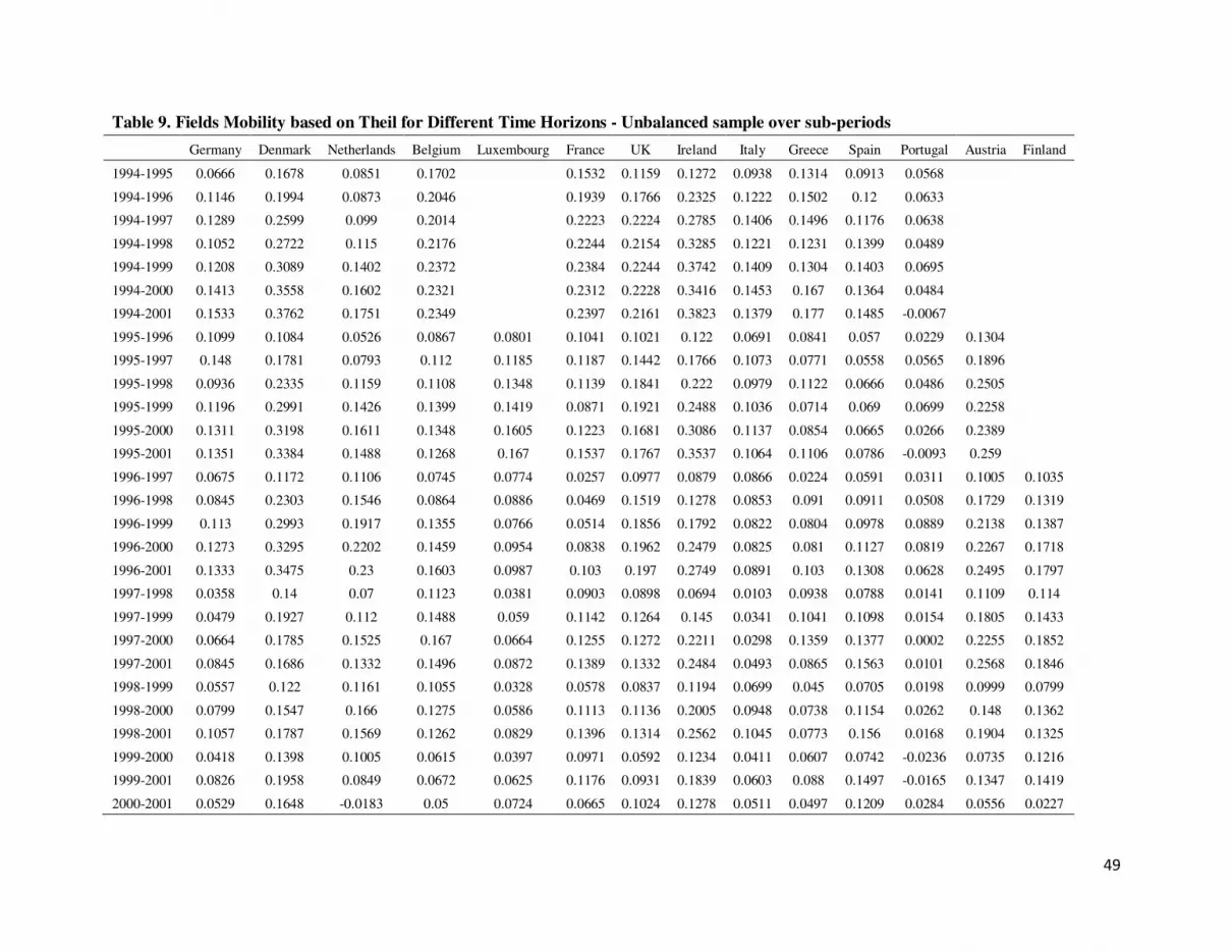
49

Table 9. Fields Mobility based on Theil for Different Time Horizons - Unbalanced sample over sub-periods

Germany Denmark Netherlands Belgium Luxembourg France UK Ireland Italy Greece Spain Portugal Austria Finland

1994-1995 0.0666 0.1678 0.0851 0.1702 0.1532 0.1159 0.1272 0.0938 0.1314 0.0913 0.0568

1994-1996 0.1146 0.1994 0.0873 0.2046 0.1939 0.1766 0.2325 0.1222 0.1502 0.12 0.0633

1994-1997 0.1289 0.2599 0.099 0.2014 0.2223 0.2224 0.2785 0.1406 0.1496 0.1176 0.0638

1994-1998 0.1052 0.2722 0.115 0.2176 0.2244 0.2154 0.3285 0.1221 0.1231 0.1399 0.0489

1994-1999 0.1208 0.3089 0.1402 0.2372 0.2384 0.2244 0.3742 0.1409 0.1304 0.1403 0.0695

1994-2000 0.1413 0.3558 0.1602 0.2321 0.2312 0.2228 0.3416 0.1453 0.167 0.1364 0.0484

1994-2001 0.1533 0.3762 0.1751 0.2349 0.2397 0.2161 0.3823 0.1379 0.177 0.1485 -0.0067

1995-1996 0.1099 0.1084 0.0526 0.0867 0.0801 0.1041 0.1021 0.122 0.0691 0.0841 0.057 0.0229 0.1304

1995-1997 0.148 0.1781 0.0793 0.112 0.1185 0.1187 0.1442 0.1766 0.1073 0.0771 0.0558 0.0565 0.1896

1995-1998 0.0936 0.2335 0.1159 0.1108 0.1348 0.1139 0.1841 0.222 0.0979 0.1122 0.0666 0.0486 0.2505

1995-1999 0.1196 0.2991 0.1426 0.1399 0.1419 0.0871 0.1921 0.2488 0.1036 0.0714 0.069 0.0699 0.2258

1995-2000 0.1311 0.3198 0.1611 0.1348 0.1605 0.1223 0.1681 0.3086 0.1137 0.0854 0.0665 0.0266 0.2389

1995-2001 0.1351 0.3384 0.1488 0.1268 0.167 0.1537 0.1767 0.3537 0.1064 0.1106 0.0786 -0.0093 0.259

1996-1997 0.0675 0.1172 0.1106 0.0745 0.0774 0.0257 0.0977 0.0879 0.0866 0.0224 0.0591 0.0311 0.1005 0.1035

1996-1998 0.0845 0.2303 0.1546 0.0864 0.0886 0.0469 0.1519 0.1278 0.0853 0.091 0.0911 0.0508 0.1729 0.1319

1996-1999 0.113 0.2993 0.1917 0.1355 0.0766 0.0514 0.1856 0.1792 0.0822 0.0804 0.0978 0.0889 0.2138 0.1387

1996-2000 0.1273 0.3295 0.2202 0.1459 0.0954 0.0838 0.1962 0.2479 0.0825 0.081 0.1127 0.0819 0.2267 0.1718

1996-2001 0.1333 0.3475 0.23 0.1603 0.0987 0.103 0.197 0.2749 0.0891 0.103 0.1308 0.0628 0.2495 0.1797

1997-1998 0.0358 0.14 0.07 0.1123 0.0381 0.0903 0.0898 0.0694 0.0103 0.0938 0.0788 0.0141 0.1109 0.114

1997-1999 0.0479 0.1927 0.112 0.1488 0.059 0.1142 0.1264 0.145 0.0341 0.1041 0.1098 0.0154 0.1805 0.1433

1997-2000 0.0664 0.1785 0.1525 0.167 0.0664 0.1255 0.1272 0.2211 0.0298 0.1359 0.1377 0.0002 0.2255 0.1852

1997-2001 0.0845 0.1686 0.1332 0.1496 0.0872 0.1389 0.1332 0.2484 0.0493 0.0865 0.1563 0.0101 0.2568 0.1846

1998-1999 0.0557 0.122 0.1161 0.1055 0.0328 0.0578 0.0837 0.1194 0.0699 0.045 0.0705 0.0198 0.0999 0.0799

1998-2000 0.0799 0.1547 0.166 0.1275 0.0586 0.1113 0.1136 0.2005 0.0948 0.0738 0.1154 0.0262 0.148 0.1362

1998-2001 0.1057 0.1787 0.1569 0.1262 0.0829 0.1396 0.1314 0.2562 0.1045 0.0773 0.156 0.0168 0.1904 0.1325

1999-2000 0.0418 0.1398 0.1005 0.0615 0.0397 0.0971 0.0592 0.1234 0.0411 0.0607 0.0742 -0.0236 0.0735 0.1216

1999-2001 0.0826 0.1958 0.0849 0.0672 0.0625 0.1176 0.0931 0.1839 0.0603 0.088 0.1497 -0.0165 0.1347 0.1419

2000-2001 0.0529 0.1648 -0.0183 0.05 0.0724 0.0665 0.1024 0.1278 0.0511 0.0497 0.1209 0.0284 0.0556 0.0227

50

Table 10. Dominance relations in long term earnings mobility: Shorrocks and Fields Index

Denmark Netherlands Belgium Luxembourg* France UK Ireland Italy Greece Spain Portugal Austria* Finland**

Germany < < < > < < < < < < > < < Shorrocks

< < < < < < < > < > > < < Fields

Denmark

> > > > > > > > > > > > Shorrocks

> > > > > < > > > > > > Fields

Netherlands

< > > < < > < > > < < Shorrocks

< >1 < < < > < > > < < Fields

Belgium

> > < > > > > > < < Shorrocks

> < > < > > > > < > Fields

Luxembourg*

< < < < < < > < < Shorrocks

< < < > <2 > > < < Fields

France

< < < < > > < < Shorrocks

> < > > > > < > Fields

UK

> > > > > < < Shorrocks

< > > > > < > Fields

Ireland

> < > > < < Shorrocks

> > > > > > Fields

Italy

< > > < < Shorrocks

< < > < < Fields

Greece

> > < < Shorrocks

> > < < Fields

Spain

> < < Shorrocks

> < < Fields

Portugal < < Shorrocks

< < Fields

Austria*

< Shorrocks

> Fields

Finland**

Note: The reading of the table goes from left to right.

(*) The comparison is based on 7-year period mobility

(**) The comparison is based on 7-year period mobility

(1) Based on the balanced approach. The reverse holds under the unbalanced approach

(2) Based on the balanced approach. Under the unbalanced approach, they are equal

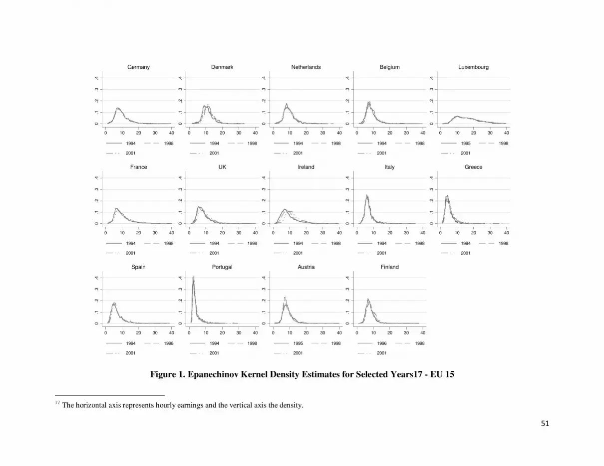
51

Figure 1. Epanechinov Kernel Density Estimates for Selected Years17 - EU 15

17 The horizontal axis represents hourly earnings and the vertical axis the density.

0.1

.2.3

.4

0 10 20 30 40

1994 1998

2001

Germany

0.1

.2.3

.4

0 10 20 30 40

1994 1998

2001

Denmark

0.1

.2.3

.4

0 10 20 30 40

1994 1998

2001

Netherlands

0.1

.2.3

.4

0 10 20 30 40

1994 1998

2001

Belgium

0.1

.2.3

.4

0 10 20 30 40

1995 1998

2001

Luxembourg

0.1

.2.3

.4

0 10 20 30 40

1994 1998

2001

France

0.1

.2.3

.4

0 10 20 30 40

1994 1998

2001

UK

0.1

.2.3

.4

0 10 20 30 40

1994 1998

2001

Ireland

0.1

.2.3

.4

0 10 20 30 40

1994 1998

2001

Italy

0.1

.2.3

.4

0 10 20 30 40

1994 1998

2001

Greece

0.1

.2.3

.4

0 10 20 30 40

1994 1998

2001

Spain

0.1

.2.3

.4

0 10 20 30 40

1994 1998

2001

Portugal0

.1.2

.3.4

0 10 20 30 40

1995 1998

2001

Austria

0.1

.2.3

.4

0 10 20 30 40

1996 1998

2001

Finland

52

Figure 2. Percentage Change in Mean Hourly Earnings by Percentiles Over The Sample

Period

Figure 3. Ratio between Mean Earnings at the 9th Decile and the 1st Decile

-20

020

40

60

10 20 30 40 50 60 70 80 90

Germany Netherlands Belgium

Luxembourg

-20

020

40

60

10 20 30 40 50 60 70 80 90

France Austria UK

Ireland Finland Denmark

-20

020

40

60

10 20 30 40 50 60 70 80 90

Italy Spain Portugal

Greece

22.5

33.5

4

Mean E

arn

ings 9

th D

ecile

/1st D

ecile

1994 1995 1996 1997 1998 1999 2000 2001

Germany Netherlands

Belgium Luxembourg

France UK

Ireland

22.5

33.5

4

Mean E

arn

ings 9

th D

ecile

/1st D

ecile

1994 1995 1996 1997 1998 1999 2000 2001

Italy Spain

Portugal Greece

Austria Finland

Denmark

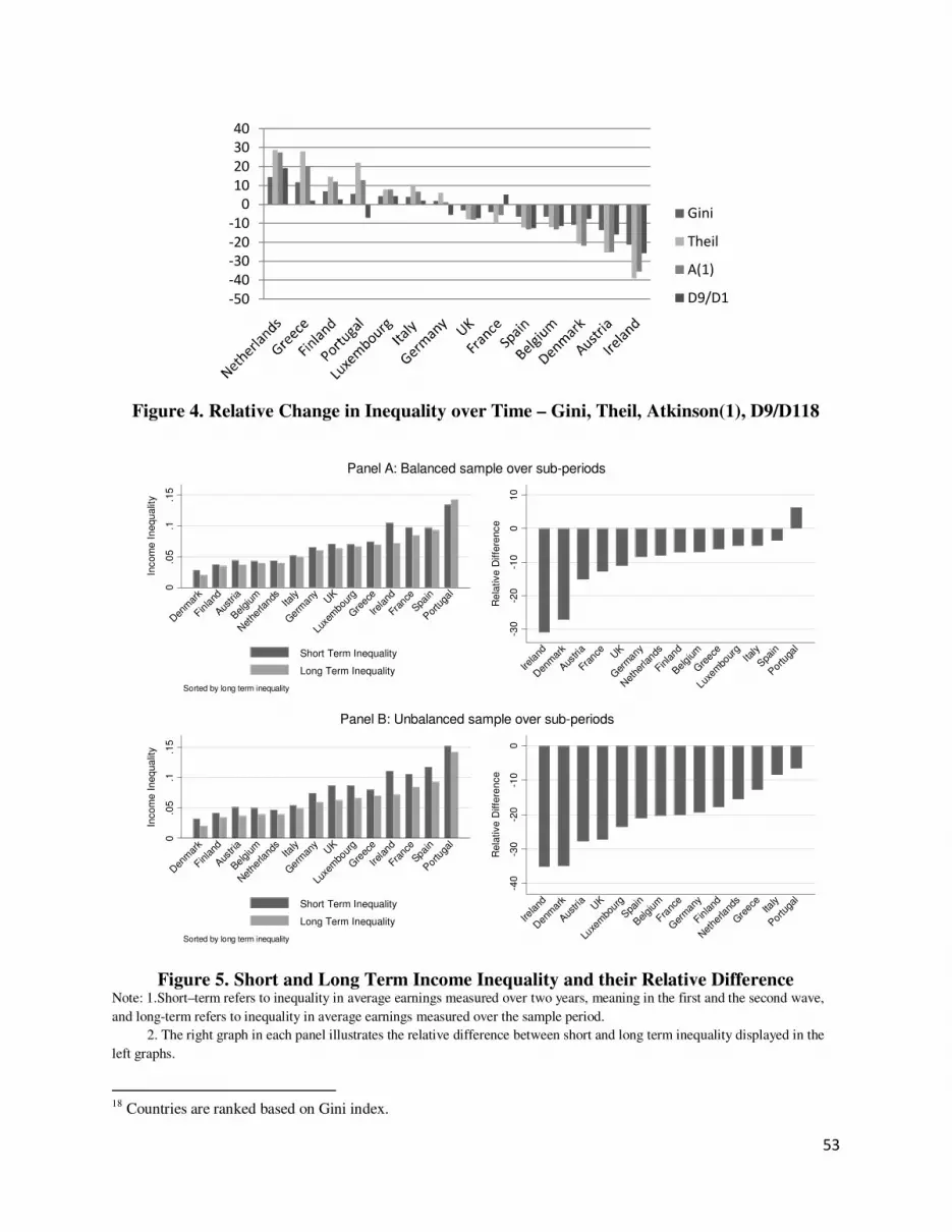
53

Figure 4. Relative Change in Inequality over Time – Gini, Theil, Atkinson(1), D9/D118

Figure 5. Short and Long Term Income Inequality and their Relative Difference

Note: 1.Short–term refers to inequality in average earnings measured over two years, meaning in the first and the second wave,

and long-term refers to inequality in average earnings measured over the sample period.

2. The right graph in each panel illustrates the relative difference between short and long term inequality displayed in the

left graphs.

18 Countries are ranked based on Gini index.

-50

-40

-30

-20

-10

0

10

20

30

40

Gini

Theil

A(1)

D9/D1

0.0

5.1

.15

Inco

me

In

eq

ua

lity

Den

mar

k

Finla

nd

Austri

a

Bel

gium

Net

herla

nds

Italy

Ger

man

yUK

Luxe

mbo

urg

Gre

ece

Irela

nd

Fran

ce

Spa

in

Por

tuga

l

Sorted by long term inequality

Short Term Inequality

Long Term Inequality

-30

-20

-10

01

0

Re

lative

Diffe

ren

ce

Irela

nd

Den

mar

k

Aus

tria

Fran

ce UK

Ger

man

y

Net

herla

nds

Finla

nd

Bel

gium

Gre

ece

Luxe

mbo

urg

Italy

Spa

in

Por

tuga

l

Panel A: Balanced sample over sub-periods

0.0

5.1

.15

Inco

me

In

eq

ua

lity

Den

mar

k

Finla

nd

Aus

tria

Belgi

um

Net

herla

nds

Italy

Ger

man

yUK

Luxe

mbo

urg

Gre

ece

Irela

nd

Fran

ce

Spain

Por

tuga

l

Sorted by long term inequality

Short Term Inequality

Long Term Inequality

-40

-30

-20

-10

0

Re

lative

Diffe

ren

ce

Irela

nd

Den

mar

k

Aus

tria

UK

Luxe

mbo

urg

Spa

in

Bel

gium

Franc

e

Ger

man

y

Finla

nd

Net

herla

nds

Gre

ece

Italy

Portu

gal

Panel B: Unbalanced sample over sub-periods

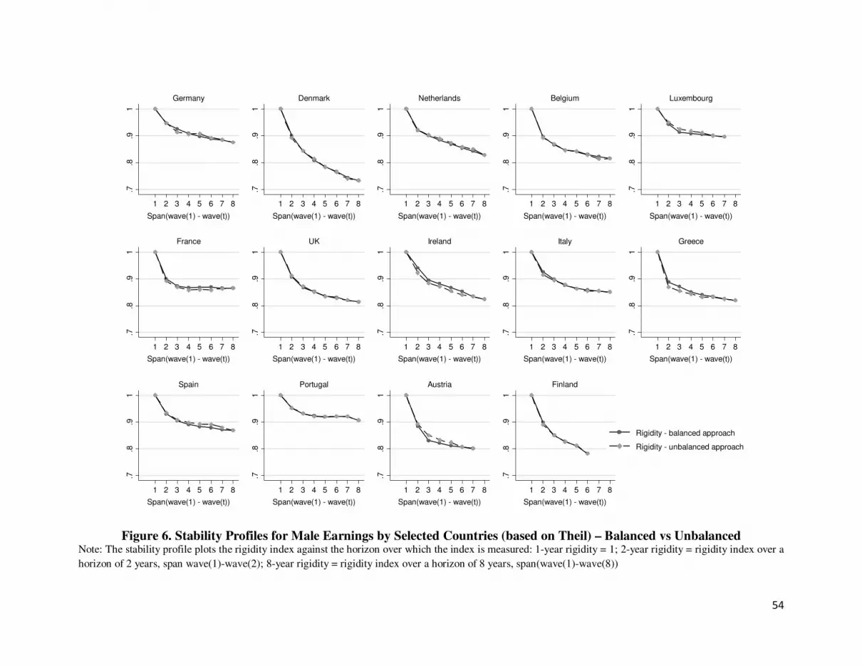
54

Figure 6. Stability Profiles for Male Earnings by Selected Countries (based on Theil) – Balanced vs Unbalanced

Note: The stability profile plots the rigidity index against the horizon over which the index is measured: 1-year rigidity = 1; 2-year rigidity = rigidity index over a

horizon of 2 years, span wave(1)-wave(2); 8-year rigidity = rigidity index over a horizon of 8 years, span(wave(1)-wave(8))

.7.8

.91

1 2 3 4 5 6 7 8

Span(wave(1) - wave(t))

Germany

.7.8

.91

1 2 3 4 5 6 7 8

Span(wave(1) - wave(t))

Denmark

.7.8

.91

1 2 3 4 5 6 7 8

Span(wave(1) - wave(t))

Netherlands

.7.8

.91

1 2 3 4 5 6 7 8

Span(wave(1) - wave(t))

Belgium

.7.8

.91

1 2 3 4 5 6 7 8

Span(wave(1) - wave(t))

Luxembourg

.7.8

.91

1 2 3 4 5 6 7 8

Span(wave(1) - wave(t))

France

.7.8

.91

1 2 3 4 5 6 7 8

Span(wave(1) - wave(t))

UK

.7.8

.91

1 2 3 4 5 6 7 8

Span(wave(1) - wave(t))

Ireland

.7.8

.91

1 2 3 4 5 6 7 8

Span(wave(1) - wave(t))

Italy

.7.8

.91

1 2 3 4 5 6 7 8

Span(wave(1) - wave(t))

Greece

.7.8

.91

1 2 3 4 5 6 7 8

Span(wave(1) - wave(t))

Spain

.7.8

.91

1 2 3 4 5 6 7 8

Span(wave(1) - wave(t))

Portugal.7

.8.9

1

1 2 3 4 5 6 7 8

Span(wave(1) - wave(t))

Austria

.7.8

.91

1 2 3 4 5 6 7 8

Span(wave(1) - wave(t))

Finland

Rigidity - balanced approach

Rigidity - unbalanced approach

55

Figure 7. Stability Profiles for Male Earnings for Selected Countries (based on Theil) - –

Balanced vs Unbalanced Note: The stability profile plots the rigidity index against the horizon over which the index is measured: 1-year

rigidity = 1; 2-year rigidity = rigidity index over a horizon of 2 years, span wave(1)-wave(2); 8-year rigidity =

rigidity index over a horizon of 8 years, span(wave(1)-wave(8))

.7.8

.91

1 2 3 4 5 6 7 8

Span(wave(1) - wave(t))

Germany Luxembourg

France Italy

Spain Portugal

.7.8

.91

1 2 3 4 5 6 7 8

Span(wave(1) - wave(t))

Denmark Netherlands Belgium

UK Ireland Greece

Austria Finland

Panel A: Balanced sample over sub-periods

.7.8

.91

1 2 3 4 5 6 7 8

Span(wave(1) - wave(t))

Germany Luxembourg

France Italy

Spain Portugal

.7.8

.91

1 2 3 4 5 6 7 8

Span(wave(1) - wave(t))

Denmark Netherlands Belgium

UK Ireland Greece

Austria Finland

Panel B: Unbalanced sample over sub-periods

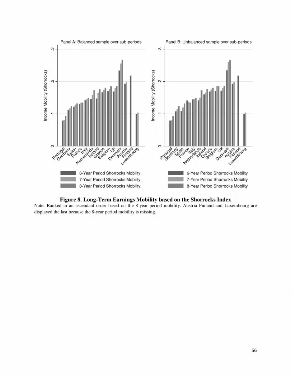
56

Figure 8. Long-Term Earnings Mobility based on the Shorrocks Index

Note: Ranked in an ascendant order based on the 8-year period mobility. Austria Finland and Luxembourg are

displayed the last because the 8-year period mobility is missing.

0.1

.2.3

Incom

e M

obili

ty (

Shorr

ocks)

Por

tuga

l

Ger

man

y

Spain

Franc

eIta

ly

Net

herla

nds

Ireland

Gre

ece

Belgi

um UK

Den

mar

k

Austri

a

Finland

Luxe

mbo

urg

Panel A: Balanced sample over sub-periods

6-Year Period Shorrocks Mobility

7-Year Period Shorrocks Mobility

8-Year Period Shorrocks Mobility

0.1

.2.3

Incom

e M

obili

ty (

Shorr

ocks)

Por

tuga

l

Ger

man

y

Spain

Franc

eIta

ly

Net

herla

nds

Ireland

Gre

ece

Belgi

um UK

Den

mar

k

Austri

a

Finland

Luxe

mbo

urg

Panel B: Unbalanced sample over sub-periods

6-Year Period Shorrocks Mobility

7-Year Period Shorrocks Mobility

8-Year Period Shorrocks Mobility

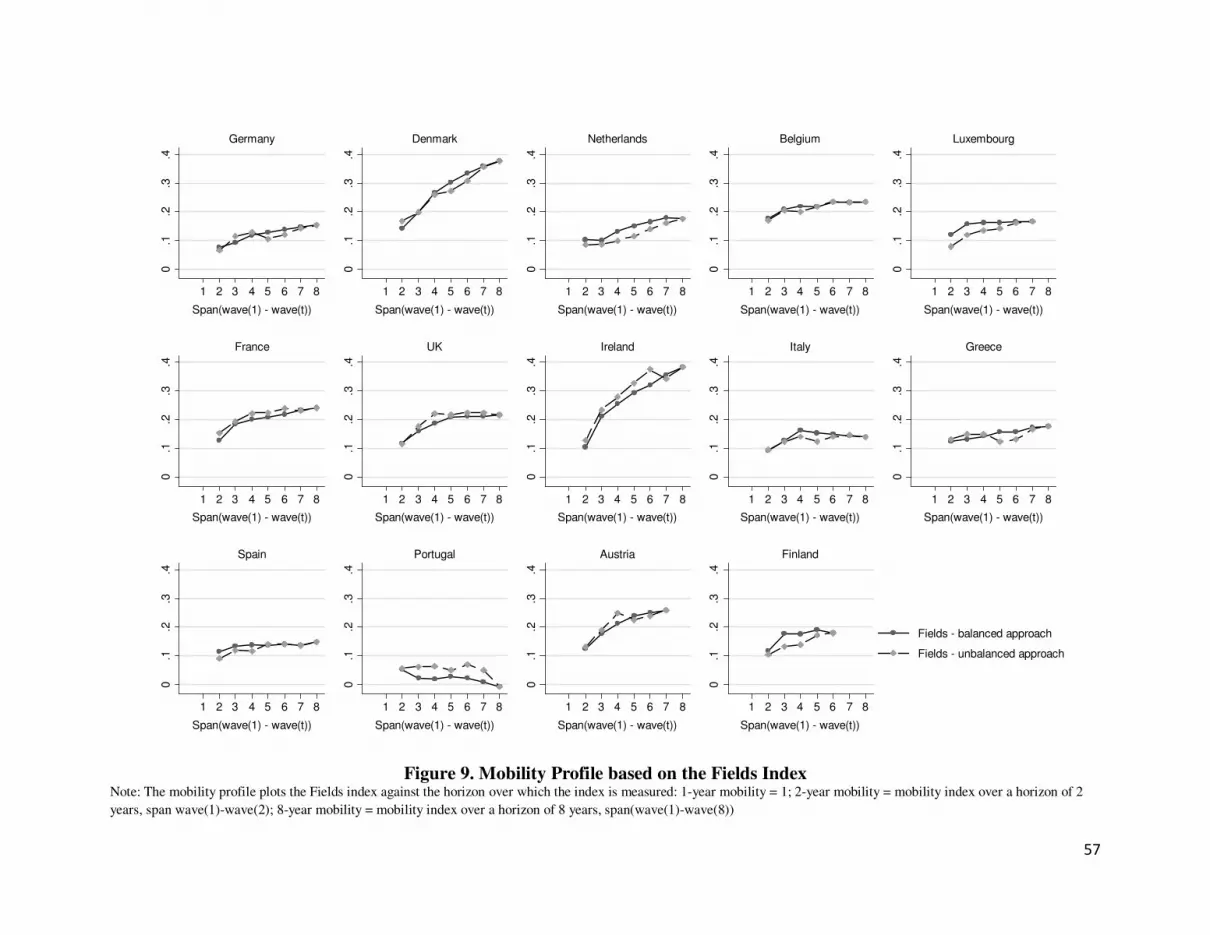
57

Figure 9. Mobility Profile based on the Fields Index

Note: The mobility profile plots the Fields index against the horizon over which the index is measured: 1-year mobility = 1; 2-year mobility = mobility index over a horizon of 2

years, span wave(1)-wave(2); 8-year mobility = mobility index over a horizon of 8 years, span(wave(1)-wave(8))

0.1

.2.3

.4

1 2 3 4 5 6 7 8

Span(wave(1) - wave(t))

Germany

0.1

.2.3

.4

1 2 3 4 5 6 7 8

Span(wave(1) - wave(t))

Denmark

0.1

.2.3

.4

1 2 3 4 5 6 7 8

Span(wave(1) - wave(t))

Netherlands

0.1

.2.3

.4

1 2 3 4 5 6 7 8

Span(wave(1) - wave(t))

Belgium

0.1

.2.3

.4

1 2 3 4 5 6 7 8

Span(wave(1) - wave(t))

Luxembourg

0.1

.2.3

.4

1 2 3 4 5 6 7 8

Span(wave(1) - wave(t))

France0

.1.2

.3.4

1 2 3 4 5 6 7 8

Span(wave(1) - wave(t))

UK

0.1

.2.3

.4

1 2 3 4 5 6 7 8

Span(wave(1) - wave(t))

Ireland

0.1

.2.3

.4

1 2 3 4 5 6 7 8

Span(wave(1) - wave(t))

Italy

0.1

.2.3

.4

1 2 3 4 5 6 7 8

Span(wave(1) - wave(t))

Greece

0.1

.2.3

.4

1 2 3 4 5 6 7 8

Span(wave(1) - wave(t))

Spain

0.1

.2.3

.4

1 2 3 4 5 6 7 8

Span(wave(1) - wave(t))

Portugal

0.1

.2.3

.4

1 2 3 4 5 6 7 8

Span(wave(1) - wave(t))

Austria

0.1

.2.3

.41 2 3 4 5 6 7 8

Span(wave(1) - wave(t))

Finland

Fields - balanced approach

Fields - unbalanced approach

58

Figure 10. Mobility Profile based on the Fields Index

Note: The mobility profile plots the Fields index against the horizon over which the index is measured: 1-year mobility = 1; 2-

year mobility = mobility index over a horizon of 2 years, span wave(1)-wave(2); 8-year mobility = mobility index over a horizon

of 8 years, span(wave(1)-wave(8))

0.1

.2.3

.4

1 2 3 4 5 6 7 8

Span(wave(1)-wave(1+t))

Germany Netherlands Luxembourg

Portugal Greece Spain

Finland

0.1

.2.3

.4

1 2 3 4 5 6 7 8

Span(wave(1)-wave(1+t))

Denmark Belgium France

UK Ireland Italy

Austria

Panel A: Balanced sample over sub-periods

0.1

.2.3

.4

1 2 3 4 5 6 7 8

Span(wave(1)-wave(1+t))

Germany Netherlands Luxembourg

Portugal Greece Spain

Finland

0.1

.2.3

.4

1 2 3 4 5 6 7 8

Span(wave(1)-wave(1+t))

Denmark Belgium France

UK Ireland Italy

Austria

Panel B: Unbalanced sample over sub-periods

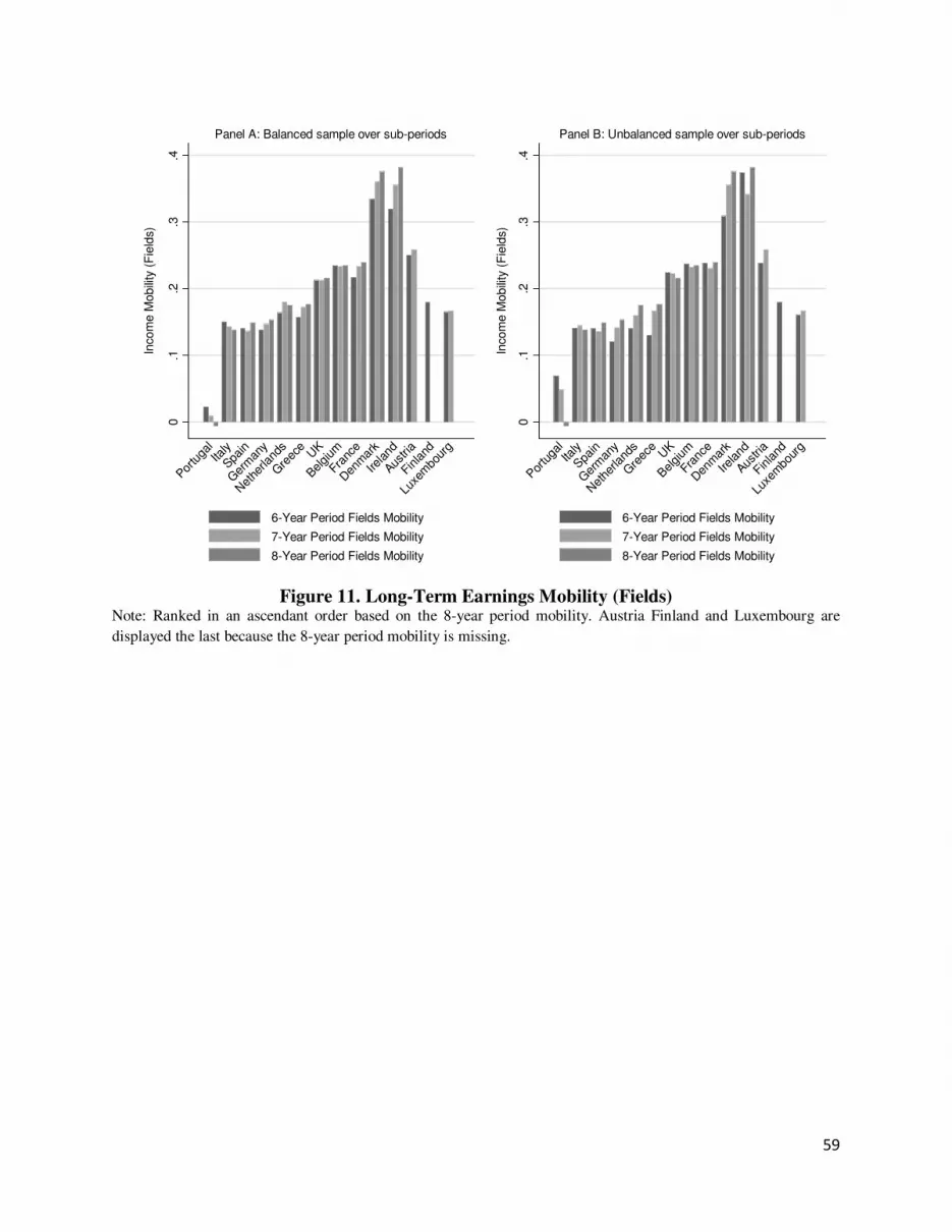
59

Figure 11. Long-Term Earnings Mobility (Fields)

Note: Ranked in an ascendant order based on the 8-year period mobility. Austria Finland and Luxembourg are

displayed the last because the 8-year period mobility is missing.

0.1

.2.3

.4

Incom

e M

obili

ty (

Fie

lds)

Portu

galIta

ly

Spain

Ger

man

y

Net

herla

nds

Gre

ece

UK

Belgium

Franc

e

Den

mar

k

Ireland

Austri

a

Finland

Luxe

mbo

urg

Panel A: Balanced sample over sub-periods

6-Year Period Fields Mobility

7-Year Period Fields Mobility

8-Year Period Fields Mobility

0.1

.2.3

.4

Incom

e M

obili

ty (

Fie

lds)

Portu

galIta

ly

Spain

Ger

man

y

Net

herla

nds

Gre

ece

UK

Belgium

Franc

e

Den

mar

k

Ireland

Austri

a

Finland

Luxe

mbo

urg

Panel B: Unbalanced sample over sub-periods

6-Year Period Fields Mobility

7-Year Period Fields Mobility

8-Year Period Fields Mobility

60

Figure 12. Scatter plot of 6-year and 7-year period mobility: Shorrocks vs. Fields

PT

GE

SP

IT

GR

NL

LU

FI

UK

F

B

AT

IR

DK.0

5.1

.15

.2.2

5

Six

-Ye

ar

Pe

rio

d S

ho

rro

cks M

ob

ility

- B

ala

nce

d

0 .1 .2 .3 .4

Six-Year Period Fields Mobility - Balanced

Panel A: Balanced sample over sub-periods

PT

GE

GR

NL

SP

IT

LU

FI

UKB

F

AT

DK

IR

.05

.1.1

5.2

.25

Six

-Ye

ar

Pe

rio

d S

ho

rro

cks M

ob

ility

0 .1 .2 .3 .4

Six-Year Period Fields Mobility

Panel B: Unbalanced sample over sub-periods

PT

SP

IT

GE

LU

GR

NL

UKB

F

AT

IR

DK

.1.1

5.2

.25

Se

ve

n-Y

ea

r P

eri

od

Sh

orr

ocks M

ob

ility

- B

ala

nce

d

0 .1 .2 .3 .4

Seven-Year Period Fields Mobility - Balanced

Panel A: Balanced sample over sub-periods

PT

SPGE

ITNL

GR

LU

UK

F

B

AT

IR

DK

.1.1

5.2

.25

Se

ve

n-Y

ea

r P

eri

od

Sh

orr

ocks M

ob

ility

0 .1 .2 .3 .4

Seven-Year Period Fields Mobility

Panel B: Unbalanced sample over sub-periods

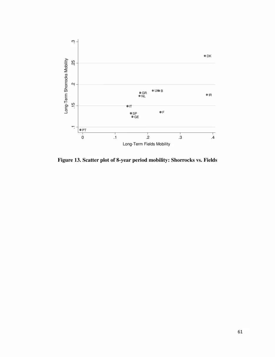
61

Figure 13. Scatter plot of 8-year period mobility: Shorrocks vs. Fields

PT

IT

SPGE

NLGR

UK B

F

DK

IR

.1.1

5.2

.25

.3

Long-T

erm

Shorr

ocks M

obili

ty

0 .1 .2 .3 .4

Long-Term Fields Mobility

62

Figure 14. The Evolution of 2-Year Period Mobility

0.0

5.1

.15

1994 1996 1998 2000

Germany

0.0

5.1

.15

1994 1996 1998 2000

Denmark

0.0

5.1

.15

1994 1996 1998 2000

Netherlands

0.0

5.1

.15

1994 1996 1998 2000

Belgium

0.0

5.1

.15

1994 1996 1998 2000

Luxembourg0

.05

.1.1

5

1994 1996 1998 2000

France

0.0

5.1

.15

1994 1996 1998 2000

UK

0.0

5.1

.15

1994 1996 1998 2000

Ireland

0.0

5.1

.15

1994 1996 1998 2000

Italy

0.0

5.1

.15

1994 1996 1998 2000

Greece

0.0

5.1

.15

1994 1996 1998 2000

Spain

0.0

5.1

.15

1994 1996 1998 2000

Portugal

0.0

5.1

.15

1994 1996 1998 2000

Austria

0.0

5.1

.15

1994 1996 1998 2000

Finland

Mobility(t, t+1)- balanced

Mobility(t, t+1)- unbalanced

2-Year Shorrocks Mobility Over Time-.

05

0.0

5.1

.15

.2

1994 1996 1998 2000

Germany

-.05

0.0

5.1

.15

.2

1994 1996 1998 2000

Denmark

-.05

0.0

5.1

.15

.2

1994 1996 1998 2000

Netherlands

-.05

0.0

5.1

.15

.2

1994 1996 1998 2000

Belgium

-.05

0.0

5.1

.15

.2

1994 1996 1998 2000

Luxembourg

-.05

0.0

5.1

.15

.2

1994 1996 1998 2000

France

-.05

0.0

5.1

.15

.2

1994 1996 1998 2000

UK

-.05

0.0

5.1

.15

.2

1994 1996 1998 2000

Ireland

-.05

0.0

5.1

.15

.2

1994 1996 1998 2000

Italy

-.05

0.0

5.1

.15

.2

1994 1996 1998 2000

Greece

-.05

0.0

5.1

.15

.2

1994 1996 1998 2000

Spain

-.05

0.0

5.1

.15

.2

1994 1996 1998 2000

Portugal

-.05

0.0

5.1

.15

.2

1994 1996 1998 2000

Austria

-.05

0.0

5.1

.15

.2

1994 1996 1998 2000

Finland

Mobility(t, t+1)- balanced

Mobility(t, t+1)- unbalanced

2-Year Fields Mobility Over Time

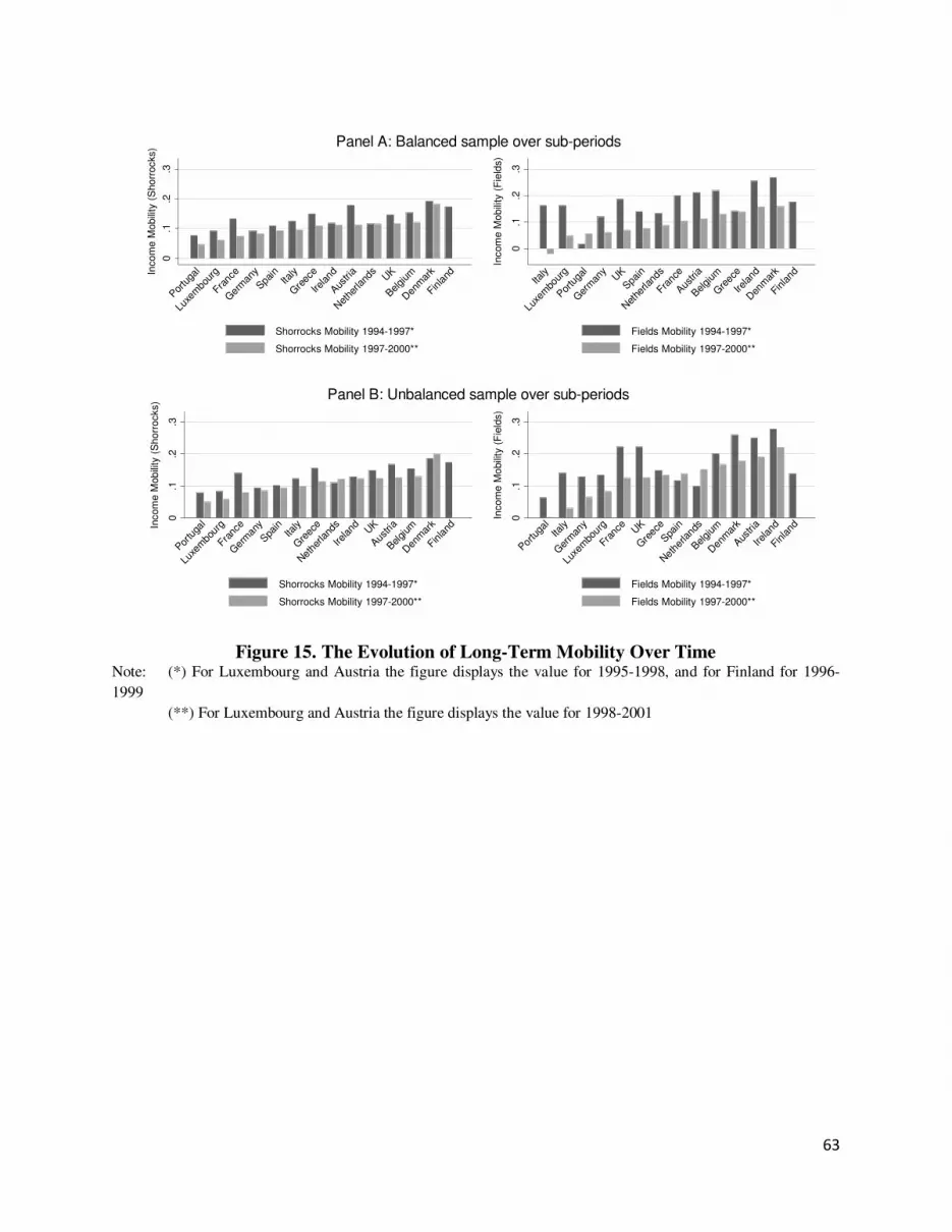
63

Figure 15. The Evolution of Long-Term Mobility Over Time

Note: (*) For Luxembourg and Austria the figure displays the value for 1995-1998, and for Finland for 1996-

1999

(**) For Luxembourg and Austria the figure displays the value for 1998-2001

0.1

.2.3

Incom

e M

obili

ty (

Shorr

ocks)

Portu

gal

Luxe

mbo

urg

Franc

e

Ger

man

y

Spain

Italy

Gre

ece

Ireland

Austri

a

Net

herla

nds

UK

Belgium

Den

mar

k

Finland

Shorrocks Mobility 1994-1997*

Shorrocks Mobility 1997-2000**

0.1

.2.3

Incom

e M

obili

ty (

Fie

lds)

Italy

Luxe

mbo

urg

Portu

gal

Ger

man

yUK

Spain

Net

herla

nds

Franc

e

Austri

a

Belgium

Gre

ece

Ireland

Den

mar

k

Finlan

d

Fields Mobility 1994-1997*

Fields Mobility 1997-2000**

Panel A: Balanced sample over sub-periods

0.1

.2.3

Incom

e M

obili

ty (

Shorr

ocks)

Portu

gal

Luxe

mbo

urg

Franc

e

Ger

man

y

Spain

Italy

Gre

ece

Nethe

rland

s

Ireland UK

Austri

a

Belgium

Den

mar

k

Finland

Shorrocks Mobility 1994-1997*

Shorrocks Mobility 1997-2000**

0.1

.2.3

Incom

e M

obili

ty (

Fie

lds)

Portu

gal

Italy

Ger

man

y

Luxe

mbo

urg

Fran

ce UK

Gre

ece

Spain

Nethe

rland

s

Belgium

Den

mar

k

Austri

a

Ireland

Finlan

d

Fields Mobility 1994-1997*

Fields Mobility 1997-2000**

Panel B: Unbalanced sample over sub-periods

64

BIBLIOGRAPHY

Aaberge, Rolf, Bjorklund, Anders, Jantti, Markus, Palme, Marten, Pedersen, Peder J., Smith, Nina, and

Wannemo, Tom. 2002. Income inequlaity and income mobility in the Scandinavian countries

compared to the United States. Review of Income and Wealth, 48(4).

Atkinson, Anthony, B., Bourguignon, Francois, and Morrisson, C. (Eds.). (1992). Empirical studies of

earnings mobility: Suisse : Harwood Academic Publishers.

Benabou, R, and Ok, E. A. 2001. Mobility and progressivity: ranking income processes according to

equality of opportunity. NBER Working Paper, 8431.

Creedy, J. 1998. The Dynamics of Inequality and Poverty. Northampton: Edward Elgar Publishing Limited.

Creedy, J., and Wilhelm, M. 2002. Income Mobility, Inequality and Social Welfare. Australian Economic

Papers, 41(2), 140-150.

Fields, Gary S. 2008. Does income mobility equalize longer-term incomes? New measures of an old

concept. Available at: http://works.bepress.com/gary_fields/23

Friedman, M. 1962. Capitalism and Freedom. Chicago: University of Chicago Press.

Friedman, Milton, and Kuznets, Simon. 1954. Income from independent professional practice. New York,

NBER

Gottschalk, Peter, and Spolaore, Enrico. 2002. On the evaluation of economic mobility. Review of

Economic Studies, 68, 191-208.

Gregg, Paul , and Vittori, Claudia 2008. Exploring Shorrocks Mobility Indices Using European Data. THE

CENTRE FOR MARKET AND PUBLIC ORGANISATION, 08(206).

Hause, John C. 1980. The fine structure of earnings and the on-the-job training hypothesis.

Econometrica, 48(4), 1013-1029.

Hofer, H., and Weber, A. 2002. Wage mobility in Austria 1986-1996? Labour Economics, 9, 563-577.

Jarvis, S., and Jenkins, S. 1998. How much income mobility is there in Britain? Economic Journal,

108(447), 428-443.

Katz, Lawrence F., and Autor, David H. 1999. Changes in the wage structure and earnings inequality. In

Handbook of Labor Economics (Vol. 3): Elsevier Science B.V.

Lillard, Lee A. 1977. The distribution of earnings and human wealth in a life-cycle context. In Cambridge

(Ed.), The Distribution of Economic Well-Being: NBER.

Mincer, Jacob. 1957. A study of income distribution. Columbia University.

Mincer, Jacob. 1958. Investment in human capital and personal income distribution. Joournal of Political

Economy, 66(4), 281-302.

Mincer, Jacob. 1962. On-the-job training: costs, returns and some implications. Journal of Political

Economy, 70(5, Part 2), S50-S79.

Mincer, Jacob. 1974. Schooling, experience and earnings. New York: NY: NBER.

OECD. 1996. Earnings inequality, low paid employment and earnings mobility. In Employment Outlook

(pp. 59-99). Paris: OECD.

OECD. 1997. Earnings mobility: taking a longer view. In Employment Outlook. Paris: OECD.

OECD. 2004. Chapter 2. Employment Protection Regulation and Labour Market Performance. In

Employment Outlook. Paris: OECD.

OECD. 2006. Labour Market Performance since 1994 and Future Challenges. In Employment Outlook.

Shorrocks, A.F. 1978. Income inequality and income mobility. Journal of Economic Theory(19), 376-393.

Sologon, Denisa M., and O'Donoghue, Cathal. 2009. Increased Opportunity to Move Up the Economic

Ladder? Earnings Mobility in EU: 1994-2001. IZA Working Series, No. 4311(July).