Advancement of Smoothness Criteria for WIM Scale Approaches

FINAL REPORT

Steven M. Kararnihas and Thomas D. Gillespie, Ph.D.

The University of Michigan Transportation Research Institute

Report UMTRI-2004- 12

June 2004

Technical Report Documentation Page 1. Report No.

UMTRI-2004- 12 2. Government Accession No. 3. Recipient's Catalog No.

4. Title and Subtitle

Advancement of Smoothness Criteria for WIM Scale Approaches

7. Author($

S. M. Karamihas and T. D. Gillespie 9. Performing Organization Name and Address

The University of Michigan Transportation Research Institute 2901 Baxter Road Ann Arbor, Michigan 48 109 12. Sponsoring Agency Name and Address

Federal Highway Administration Turner-Fairbank Highway Research Center 6300 Georgetown Pike, HRDI-13 McLean, VA 22101-2296

15. Supplementary Notes

5. Report Date

April 2004 6 . Performing Organization Code

047056lF009773 8. Performing Organization Repon No.

UMTRI-2004- 12

10. Work Unit No. (TRAIS)

,,, Contract or Grant No,

13. Type of Report and Period Covered

Final Report August 2003 - July 2004

14. Sponsoring Agency Code

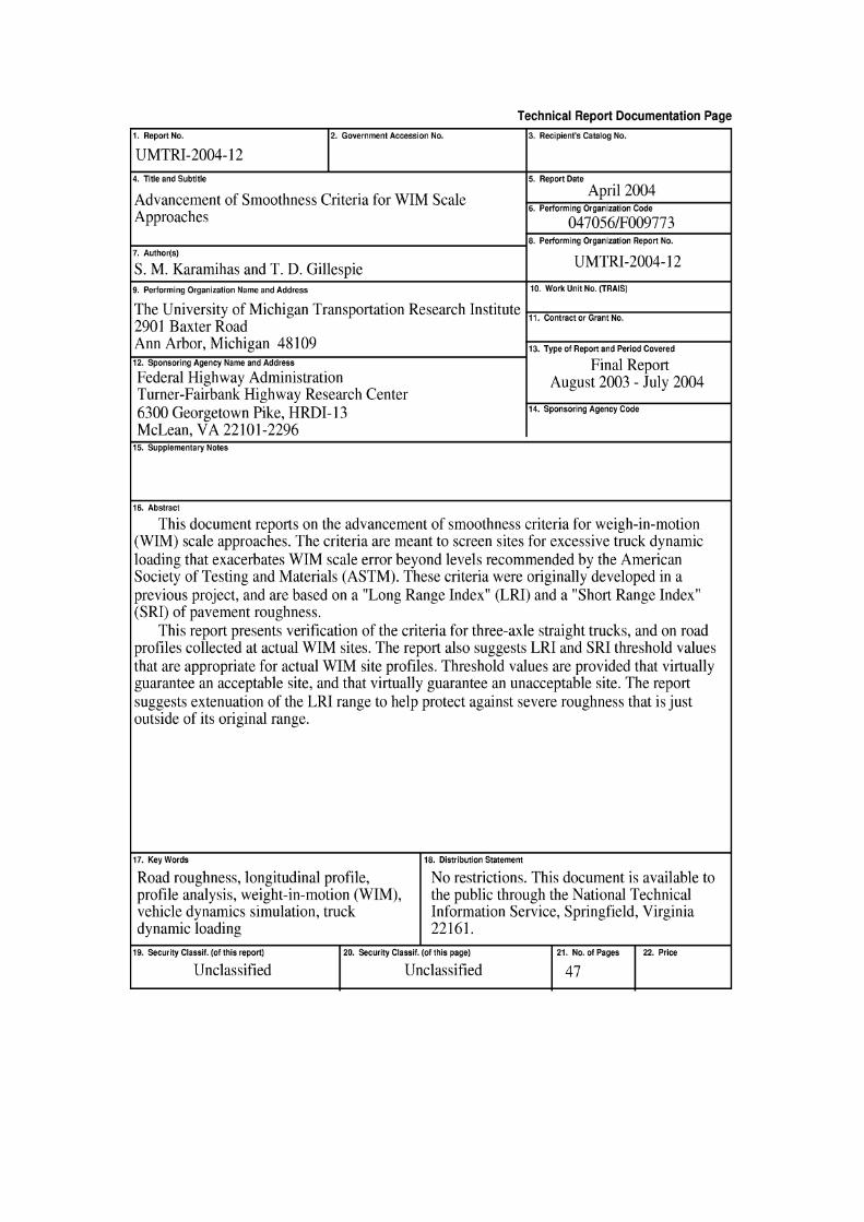
16. Abstract

This document reports on the advancement of smoothness criteria for weigh-in-motion (WIM) scale approaches. The criteria are meant to screen sites for excessive truck dynamic loading that exacerbates WIM scale error beyond levels recommended by the American Society of Testing and Materials (ASTM). These criteria were originally developed in a previous project, and are based on a "Long Range Index" (LRI) and a "Short Range Index" (SRI) of pavement roughness.

This report presents verification of the criteria for three-axle straight trucks, and on road profiles collected at actual WIM sites. The report also suggests LRI and SRI threshold values that are appropriate for actual WIM site profiles. Threshold values are provided that virtually guarantee an acceptable site, and that virtually guarantee an unacceptable site. The report suggests extenuation of the LRI range to help protect against severe roughness that is just outside of its original range.

17. Key Words

Road roughness, longitudinal profile, profile analysis, weight-in-motion (WIM), vehicle dynamics simulation, truck dynamic loading

18. Distribution Statement

No restrictions. This document is available to the public through the National Technical Information Service, Springfield, Virginia 22161.

19. Security Ciassif. (of this report)

Unclassified 20. Security Ciassif. (of this page)

Unclassified 21. NO. of Pages

47 22. Price

LIST OF FIGURES

Figure 1 . WIM error levels versus LRI and SRI ................................................... 3 Figure 2 . Development of threshold values of LRI and SRI ........................ .. .... 4 Figure 3 . Scale performance for 3-axle straight trucks vs . LRI and SRI ............... 7 Figure 4 . Narrow dips near a WIM scale .............. .. ...... ............. ........................... 9 Figure 5 . Elevation change at a WIM scale ........................................................... 9 Figure 6 . Scale performance for 5-axle tractor semitrailers on WIM sites ............ 13 Figure 7 . Scale performance compared to peak SRI ............................................. 15

............................................................................. Figure 8 . Peak SRI calculation -16 Figure 9 . Scale error caused by a step ................................................................... 18 Figure 10 . Scale error caused by a slope break ................................. .... ........ 18

............................................................................. Figure 11 . Inspection of LRI 19 Figure A-1 . Best fit logarithmic model ................. ................. ................................ 22

......................................... Figure A-2 . 95 percent confidence limits on the model 23 ............................................ Figure A-3 . 95 percent confidence limits on the data 24

........................................................................... Figure C- 1 . Degrees of freedom 35 Figure C-2 . Sample truck suspension force-deflection measurement .................... 36 Figure C-3 . Sample spring boundary tables .......................................................... 36 Figure C-4 . Four-spring suspension schematic ................................................... 37 Figure C-5 . Walking-beam suspension schematic ................................................ 38

LIST OF TABLES

.............................................................. Table 1 . WIM Scale Error Index Details 1 Table 2 . Roughness Index Thresholds. Five-Axle Tractor Semitrailers ................. 5 Table 3 . Roughness Index Thresholds. Three-Axle Straight Trucks ..................... 8

.......................................... Table 4 . WIM site profile scale performance. left side 11 Table 4 (cont) . WIM site profile scale performance. right side ........................... 12 Table 5 . Roughness Index Thresholds. WIM Site Profiles ................................... 14 Table 6 . Roughness Index Thresholds. WIM Site Profiles ........... ... .............. 15

......................................... Table 7 . Recommended Roughness Index Thresholds 20 . .................................................................................. Table B-1 WIM sites 27

.................................................. Table B-2 . WIM site profile roughness. left side 28 Table B-2 (cont) . WIM site profile roughness. right side ..................................... 29

................................................. Table D- 1 . Suspensions and Unsprung Weight 41 Table D-2 . Standard Tire Stiffness Values ............................................................ 42 Table D-3 . Vehicle Wheelbase and Weight Distribution .................... ... .......... 43 Table D-4 . Suspension Combinations and Loading Schemes ............................... 44

INTRODUCTION

The purpose of this project was to advance the development of smoothness specifications for weigh in motion (WIM) scale approaches. The smoothness specifications were originally developed for the Federal Highway Administration (FHWA) for use on WIM scales at Long-Term Pavement Performance (LTPP) study Specific Pavement Studies (SPS) sites. (1)

The original project based the smoothness criteria for acceptable WIM approach pavement on simulation of truck dynamic loading over measured road profiles. The project simulated a population of 1,232 five-axle tractor semitrailers on 61 road profiles at three speeds. The trucks were simulated in the pitch plane. The truck population included typical tractor, trailer, loading, and suspension combinations. The profiles included four surface types: jointed plain Portland cement concrete (PCC), jointed reinforced PCC, asphalt overlay on PCC, and full-depth asphalt. The entire population of trucks ran over each profile at three speeds. The distributions of WIM scale error associated with dynamic load variations were compiled for a designated scale location within each profile. Three distributions were compiled: steering axle error, tandem axle error, and gross weight error.

The original project sought a profile-based roughness index that could predict the 95th percentile error level in steering axle weight, tandem axle weight, and gross vehicle weight. The research showed that two roughness indices were needed. The first characterized the "background" roughness for a relatively long distance leading up to the scale and a short distance beyond it. This was given the name Long Range Index (LRI). The second characterized roughness directly at the scale. This was given the name Short Range Index (SRI). Both of these were based on a four-pole Butterworth band-pass filter. ( 2 ) Table 1 summarizes the index. A full description of the index is provided in a previous report. (I)

Table 1. WIM Scale Error Index Details.

Threshold values were set for both indices that would virtually ensure compliance of a site with the American Society of Testing and Materials (ASTM) standard for Type I WIM scale performance. (3) The ASTM criteria require that a WIM scale is able to measure steering axle weight within 20 percent, tandem axle weight within 15 percent, and gross vehicle weight within 10 percent with 95 percent confidence. The research showed that the tandem axle and gross vehicle weight criteria were usually violated simultaneously, and that the steering axle weight criteria was never violated unless the others were violated also.

Criterion

Long Range Short Range

In this project, the criteria were validated with further simulations, and modified to improve their relevance. This report describes the results of the following analyses:

Pavement Range Filter Cutoff Values

Examination of Index Threshold Values: The suggested threshold values for LRI and SRI in the original report were 0.789 m/km. These were established by visual inspection of the relationship between predicted scale performance and the index

Start (m) -25.8 -2.74

End (m) 3.20 0.46

Short (m) 1.08 1.56

Long (m) 11.37 16.45

values. In this project, more rigorous statistical methods are used to establish new thresholds.

Verification of the Criteria for Another Vehicle Type: The smoothness criteria were originally developed for simulated five-axle tractor semitrailers. This project compared simulated scale performance to the LRI and SRI for a population of three- axle straight trucks over the same profiles.

Study of the Criteria on Actual WIM Site Profiles: The smoothness criteria were originally developed using profiles that were not collected at actual WIM sites. Since then, data have been collected at 39 SPS WIM sites using the LTPP protocol. This project compared simulated scale performance on these sites to the LRI and SRI to demonstrate their validity on pavement that appears near WIM scales.

Revision of the LRI Range: The LRI at a given location is sensitive to profile features from 25.8 m upstream of the scale to 3.2 m beyond it. The (25.8-m) range ahead of the scale is much shorter than simple analysis of truck dynamic behavior would suggest. As a remedy, this report recommends that the LRI obey a given threshold over at least a 30-m range of pavement leading up to the scale. When this is combined with the 25.8-m "reach" of the index, a minimum of 55.8 m of pavement ahead of the scale will be considered.

EXAMINATION OF INDEX THRESHOLD VALUES

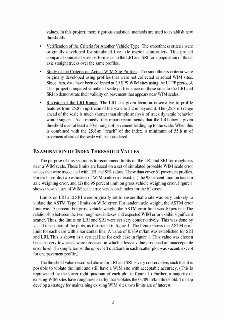
The purpose of this section is to recommend limits on the LRI and SRI for roughness near a WIM scale. These limits are based on a set of simulated probable WIM scale error values that were associated with LRI and SRI values. These data cover 61 pavement profiles. For each profile, two estimates of WIM scale error exist: (I) the 95 percent limit on tandem axle weighing error, and (2) the 95 percent limit on gross vehicle weighing error. Figure 1 shows these values of WIM scale error versus each index for the 61 cases.

Limits on LRI and SRI were originally set to ensure that a site was very unlikely to violate the ASTM Type I limits on WIM error. For tandem axle weight, the ASTM error limit was 15 percent. For gross vehicle weight, the ASTM error limit was 10 percent. The relationship between the two roughness indexes and expected WIM error exhibit significant scatter. Thus, the limits on LRI and SRI were set very conservatively. This was done by visual inspection of the plots, as illustrated in figure 1. The figure shows the ASTM error limit for each case with a horizontal line. A value of 0.789 m/km was established for SRI and LRI. This is shown as a vertical line for each case in figure 1. This value was chosen because very few cases were observed in which a lesser value produced an unacceptable error level. (In simple terms, the upper left quadrant in each scatter plot was vacant, except for one pavement profile.)

The threshold value described above for LRI and SRI is very conservative, such that it is possible to violate the limit and still have a WIM site with acceptable accuracy. (This is represented by the lower right quadrant of each plot in figure I.) Further, a majority of existing WIM sites have roughness nearby that violates the 0.789 m/km threshold. To help develop a strategy for maintaining existing WIM sites, two limits are of interest:

a lower threshold on LRI and SRI, beneath which the site is very likely to produce an acceptable level of weighing error, and

an upper threshold on LRI and SRI, above which a site is very likely to produce an unacceptable level of weighing error.

95 Percentile Tandem Axle Error 95 Percentile Gross Weight Error

a a a

% @

@.error limit

error limit

I 0 ~ I I I I I O ~ I I I I I

0.0 .5 1.0 1.5 2.0 2.5 3.0 0.0 .5 1.0 1.5 2.0 2.5 3.0 LRI (rdkm) LRI ( d m )

95 Percentile Tandem Axle Error 95 Percentile Gross Weight Error

error limit error limit

0.0 .5 1.0 1.5 2.0 2.5 3.0 3.5 0.0 .5 1.0 1.5 2.0 2.5 3.0 3.5 SRI (rdkm) SRI (rdkm)

Figure 1. WIM error levels versus LRI and SRI.

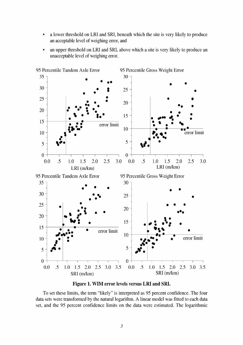
To set these limits, the term "likely" is interpreted as 95 percent confidence. The four data sets were transformed by the natural logarithm. A linear model was fitted to each data set, and the 95 percent confidence limits on the data were estimated. The logarithmic

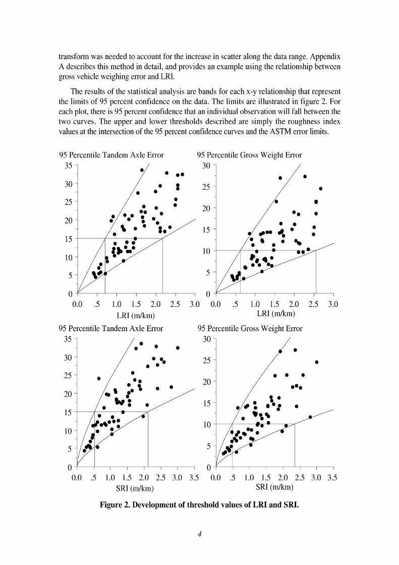
transform was needed to account for the increase in scatter along the data range. Appendix A describes this method in detail, and provides an example using the relationship between gross vehicle weighing error and LRI.

The results of the statistical analysis are bands for each x-y relationship that represent the limits of 95 percent confidence on the data. The limits are illustrated in figure 2. For each plot, there is 95 percent confidence that an individual observation will fall between the two curves. The upper and lower thresholds described are simply the roughness index values at the intersection of the 95 percent confidence curves and the ASTM error limits.

95 Percentile Tandem Axle Error 95 Percentile Gross Weight Error

0.0 .5 1.0 1.5 2.0 2.5 3.0 0.0 .5 1.0 1.5 2.0 2.5 3.0 LRI ( d k m ) LRI (mtkm)

95 Percentile Tandem Axle Error 95 Percentile Gross Weight Error

0.0 .5 1.0 1.5 2.0 2.5 3.0 3.5 0.0 .5 1.0 1.5 2.0 2.5 3.0 3.5 SRI ( d k m ) SRI ( d k m )

Figure 2. Development of threshold values of LRI and SRI.

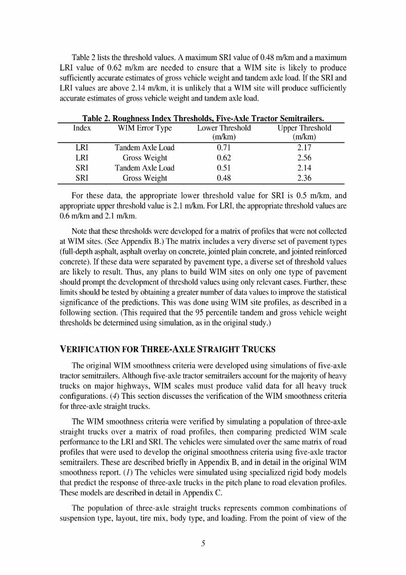
Table 2 lists the threshold values. A maximum SRI value of 0.48 dkm and a maximum LRI value of 0.62 m/km are needed to ensure that a WIM site is likely to produce sufficiently accurate estimates of gross vehicle weight and tandem axle load. If the SRI and LRI values are above 2.14 m/km, it is unlikely that a WIM site will produce sufficiently accurate estimates of gross vehicle weight and tandem axle load.

Table 2. Roughness Index Thresholds, Five-Axle Tractor Semitrailers. Index WIM Error Type Lower Threshold Upper Threshold

( h ) ( h ) LRI Tandem Axle Load 0.71 2.17 LRI Gross Weight 0.62 2.56 SRI Tandem Axle Load 0.5 1 2.14 SRI Gross Weight 0.48 2.36

For these data, the appropriate lower threshold value for SRI is 0.5 mlkm, and appropriate upper threshold value is 2.1 m/km. For LRI, the appropriate threshold values are 0.6 dkm and 2.1 dkm.

Note that these thresholds were developed for a matrix of profiles that were not collected at WIM sites. (See Appendix B.) The matrix includes a very diverse set of pavement types (full-depth asphalt, asphalt overlay on concrete, jointed plain concrete, and jointed reinforced concrete). If these data were separated by pavement type, a diverse set of threshold values are likely to result. Thus, any plans to build WIM sites on only one type of pavement should prompt the development of threshold values using only relevant cases. Further, these limits should be tested by obtaining a greater number of data values to improve the statistical significance of the predictions. This was done using WIM site profiles, as described in a following section. (This required that the 95 percentile tandem and gross vehicle weight thresholds be determined using simulation, as in the original study.)

VERIFICATION FOR THREE-AXLE STRAIGHT TRUCKS

The original WIM smoothness criteria were developed using simulations of five-axle tractor semitrailers. Although five-axle tractor semitrailers account for the majority of heavy trucks on major highways, WIM scales must produce valid data for all heavy truck configurations. (4) This section discusses the verification of the WIM smoothness criteria for three-axle straight trucks.

The WIM smoothness criteria were verified by simulating a population of three-axle straight trucks over a matrix of road profiles, then comparing predicted WIM scale performance to the LRI and SRI. The vehicles were simulated over the same matrix of road profiles that were used to develop the original smoothness criteria using five-axle tractor semitrailers. These are described briefly in Appendix B, and in detail in the original WIM smoothness report. ( I ) The vehicles were simulated using specialized rigid body models that predict the response of three-axle trucks in the pitch plane to road elevation profiles. These models are described in detail in Appendix C.

The population of three-axle straight trucks represents common combinations of suspension type, layout, tire mix, body type, and loading. From the point of view of the

models, layout, body type, and loading simply determine the location of the axle, the weight supported at each axle, and the mass distribution (i.e., pitch moment of inertia). Suspension type and tire mix determine the stiffness and damping of each compliant element. The set of trucks includes 218 combinations of vehicle properties. These are described in detail in Appendix D.

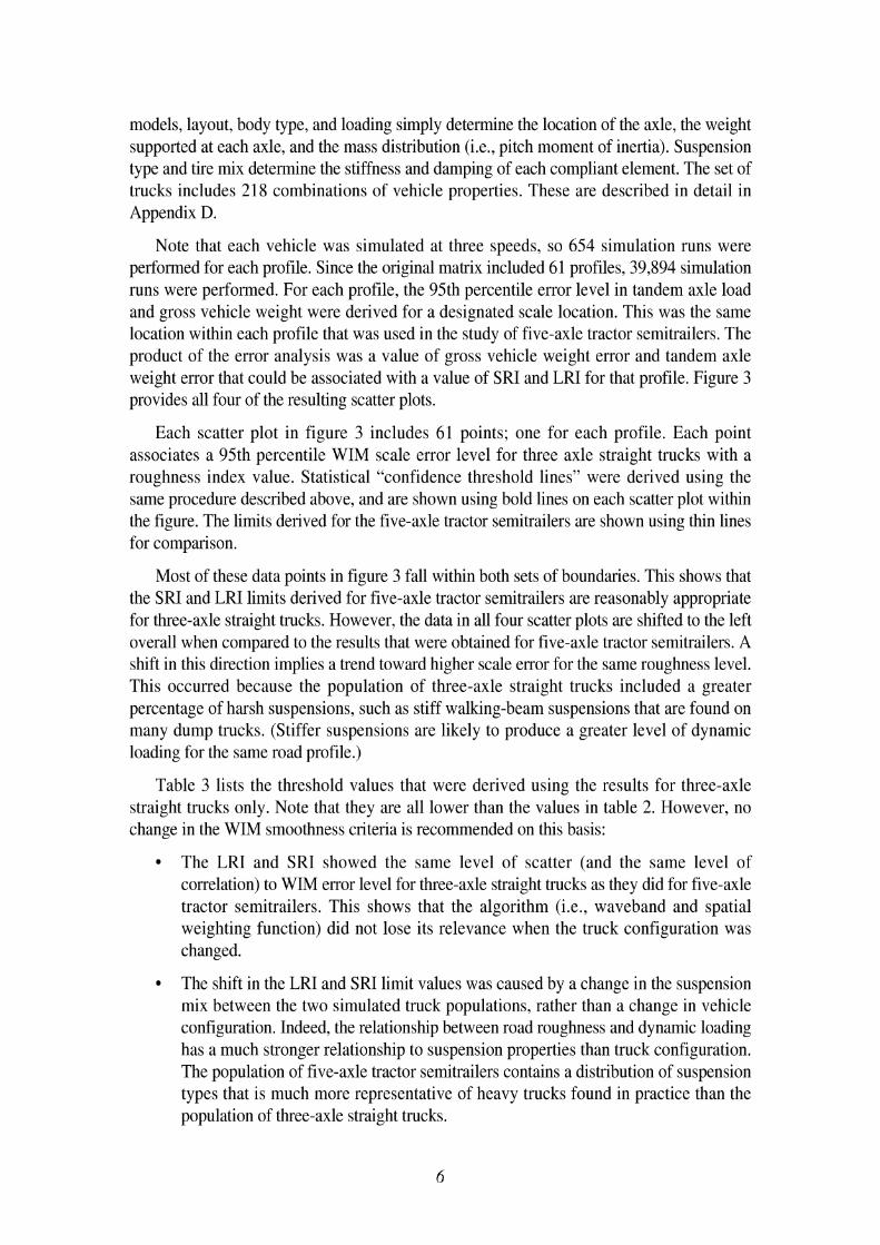
Note that each vehicle was simulated at three speeds, so 654 simulation runs were performed for each profile. Since the original matrix included 61 profiles, 39,894 simulation runs were performed. For each profile, the 95th percentile error level in tandem axle load and gross vehicle weight were derived for a designated scale location. This was the same location within each profile that was used in the study of five-axle tractor semitrailers. The product of the error analysis was a value of gross vehicle weight error and tandem axle weight error that could be associated with a value of SRI and LRI for that profile. Figure 3 provides all four of the resulting scatter plots.

Each scatter plot in figure 3 includes 61 points; one for each profile. Each point associates a 95th percentile WIM scale error level for three axle straight trucks with a roughness index value. Statistical "confidence threshold lines" were derived using the same procedure described above, and are shown using bold lines on each scatter plot within the figure. The limits derived for the five-axle tractor semitrailers are shown using thin lines for comparison.

Most of these data points in figure 3 fall within both sets of boundaries. This shows that the SRI and LRI limits derived for five-axle tractor semitrailers are reasonably appropriate for thee-axle straight tiucks. However, the data in all four scatter plots are shifted to the left overall when compared to the results that were obtained for five-axle tractor semitrailers. A shift in this direction implies a trend toward higher scale error for the same roughness level. This occurred because the population of three-axle straight trucks included a greater percentage of harsh suspensions, such as stiff walking-beam suspensions that are found on many dump trucks. (Stiffer suspensions are likely to produce a greater level of dynamic loading for the same road profile.)

Table 3 lists the threshold values that were derived using the results for three-axle straight trucks only. Note that they are all lower than the values in table 2. However, no change in the WIM smoothness criteria is recommended on this basis:

The LRI and SRI showed the same level of scatter (and the same level of correlation) to WIM error level for thee-axle straight tsucks as they did for five-axle tractor semitrailers. This shows that the algorithm (i.e., waveband and spatial weighting function) did not lose its relevance when the truck configuration was changed.

The shift in the LRI and SRI limit values was caused by a change in the suspension mix between the two simulated truck populations, rather than a change in vehicle configuration. Indeed, the relationship between road roughness and dynamic loading has a much stronger relationship to suspension properties than truck configuration. The population of five-axle tractor semitrailers contains a distribution of suspension types that is much more representative of heavy trucks found in practice than the population of three-axle straight tsucks.

Five-axle tractor semitrailers make up a much greater portion of the overall vehicle population than three-axle straight trucks, especially in terms of vehicle miles traveled. (4) If results for both truck configurations were combined and weighted to reflect their relative contribution to the truck population, the modest shift in limit value shown in table 3 would be reduced significantly.

95 Percentile Tandem Axle Error 95 Percentile Gross Weight Error

0.0 .5 1.0 1.5 2.0 2.5 3.0 0.0 .5 1.0 1.5 2.0 2.5 3.0 LRI ( d k m ) LRI (mtkm)

95 Percentile Tandem Axle Error 95 Percentile Gross Weight Error

0.0 .5 1.0 1.5 2.0 2.5 3.0 0.0 .5 1.0 1.5 2.0 2.5 3.0 3.5 SRI ( d k m ) SRI ( d k m )

Figure 3. Scale performance for 3-axle straight trucks vs. LRI and SRI.

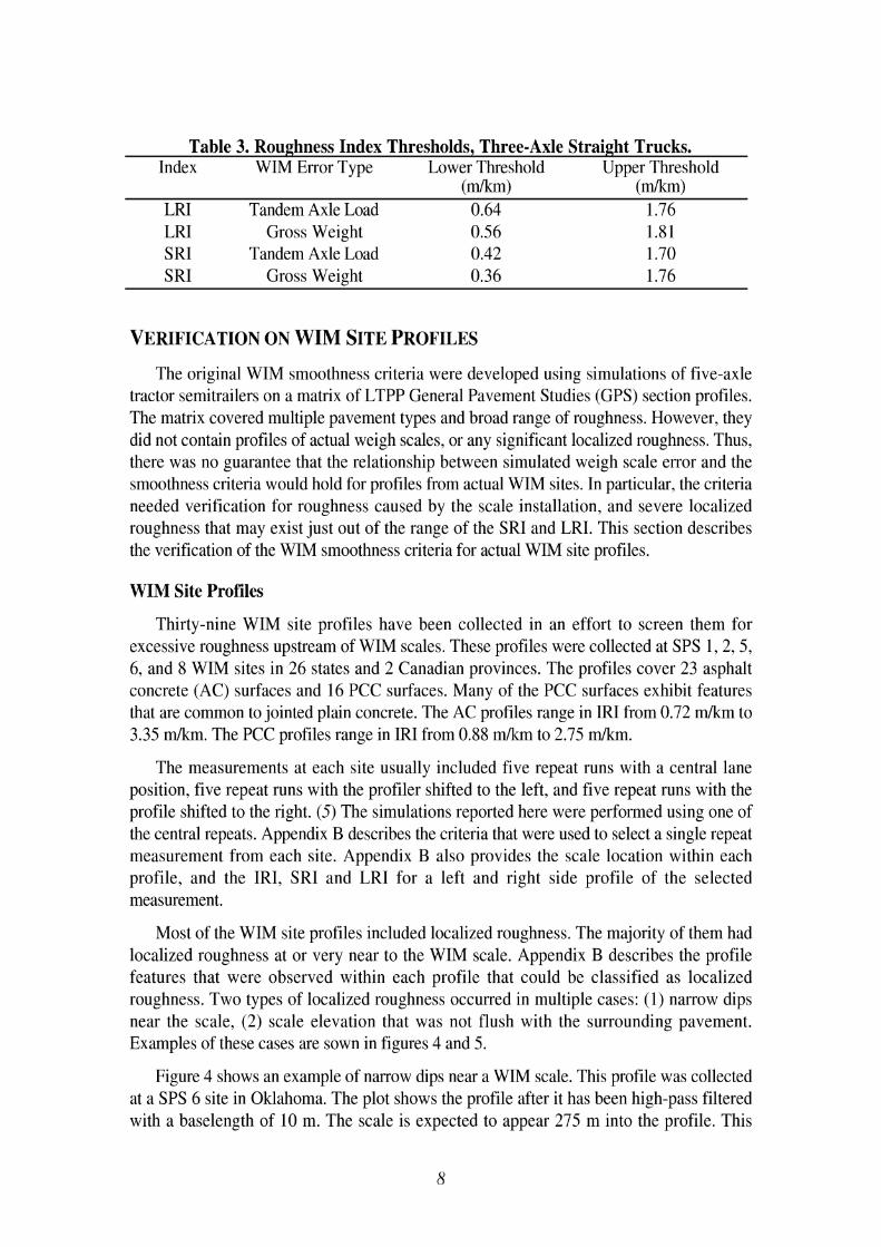
Table 3. Roughness Index Thresholds, Three-Axle Straight Trucks. Index WIM Error Type Lower Threshold Upper Threshold

(mlkm) (mlkm) LRI Tandem Axle Load 0.64 1.76 LRI Gross Weight 0.56 1.81 SRI Tandem Axle Load 0.42 1.70 SRI Gross Weight 0.36 1.76

VERIFICATION ON WIM SITE PROFILES

The original WIM smoothness criteria were developed using simulations of five-axle tractor semitrailers on a matrix of LTPP General Pavement Studies (GPS) section profiles. The matrix covered multiple pavement types and broad range of roughness. However, they did not contain profiles of actual weigh scales, or any significant localized roughness. Thus, there was no guarantee that the relationship between simulated weigh scale error and the smoothness criteria would hold for profiles from actual WIM sites. In particular, the criteria needed verification for roughness caused by the scale installation, and severe localized roughness that may exist just out of the range of the SRI and LRI. This section describes the verification of the WIM smoothness criteria for actual WIM site profiles.

WIM Site Profiles

Thirty-nine WIM site profiles have been collected in an effort to screen them for excessive roughness upstream of WIM scales. These profiles were collected at SPS 1 ,2 ,5 , 6, and 8 WIM sites in 26 states and 2 Canadian provinces. The profiles cover 23 asphalt concrete (AC) surfaces and 16 PCC surfaces. Many of the PCC surfaces exhibit features that are common to jointed plain concrete. The AC profiles range in IRI from 0.72 d k m to 3.35 m/km. The PCC profiles range in IRI from 0.88 m/km to 2.75 mkm.

The measurements at each site usually included five repeat runs with a central lane position, five repeat runs with the profiler shifted to the left, and five repeat runs with the profile shifted to the right. (5) The simulations reported here were performed using one of the central repeats. Appendix B describes the criteria that were used to select a single repeat measurement from each site. Appendix B also provides the scale location within each profile, and the IRI, SRI and LRI for a left and right side profile of the selected measurement.

Most of the WIM site profiles included localized roughness. The majority of them had localized roughness at or very near to the WIM scale. Appendix B describes the profile features that were observed within each profile that could be classified as localized roughness. Two types of localized roughness occurred in multiple cases: (1) narrow dips near the scale, (2) scale elevation that was not flush with the surrounding pavement. Examples of these cases are sown in figures 4 and 5.

Figure 4 shows an example of narrow dips near a WIM scale. This profile was collected at a SPS 6 site in Oklahoma. The plot shows the profile after it has been high-pass filtered with a baselength of 10 m. The scale is expected to appear 275 m into the profile. This

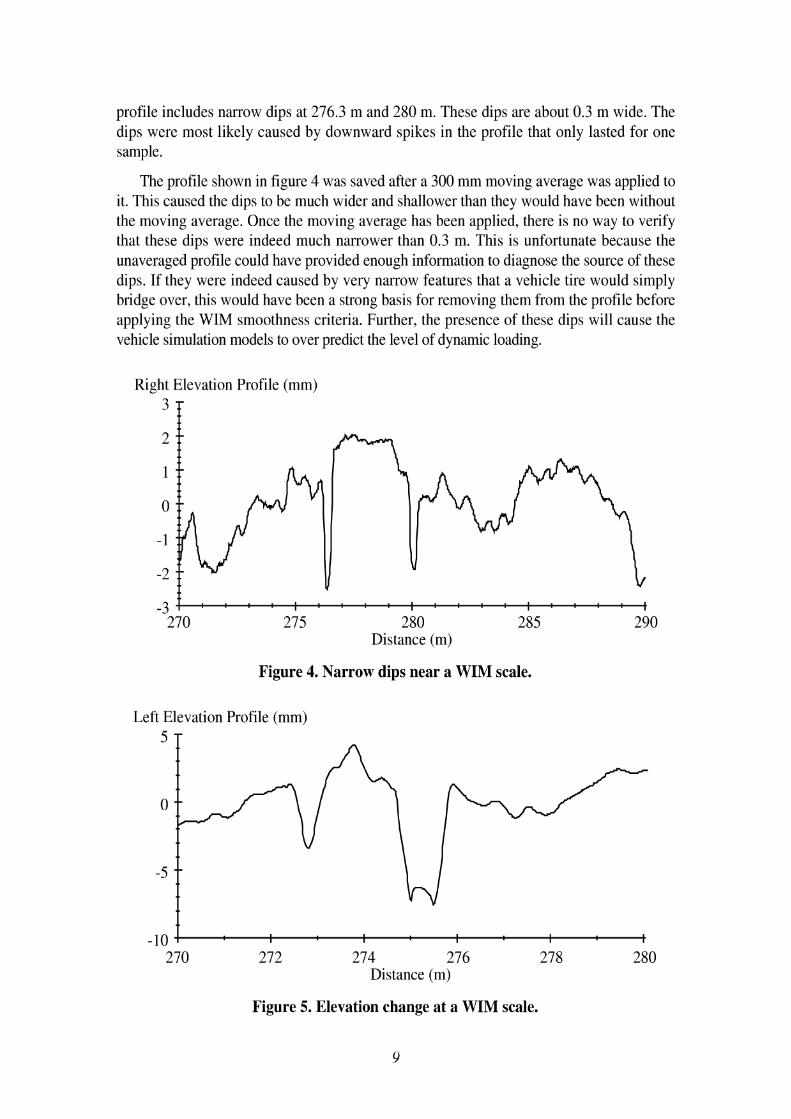
profile includes narrow dips at 276.3 m and 280 m. These dips are about 0.3 m wide. The dips were most likely caused by downward spikes in the profile that only lasted for one sample.

The profile shown in figure 4 was saved after a 300 mm moving average was applied to it. This caused the dips to be much wider and shallower than they would have been without the moving average. Once the moving average has been applied, there is no way to verify that these dips were indeed much narrower than 0.3 m. This is unfortunate because the unaveraged profile could have provided enough information to diagnose the source of these dips. If they were indeed caused by very narrow features that a vehicle tire would simply bridge over, this would have been a strong basis for removing them from the profile before applying the WIM smoothness criteria. Further, the presence of these dips will cause the vehicle simulation models to over predict the level of dynamic loading.

Right Elevation Profile (mm)

T

270 275 280 285 290 Distance (m)

Figure 4. Narrow dips near a WIM scale.

Left Elevation Profile (mm) 5 -

-5 --

-10 I I I I t 270 272 274 276 278 280

Distance (m)

Figure 5. Elevation change at a WIM scale.

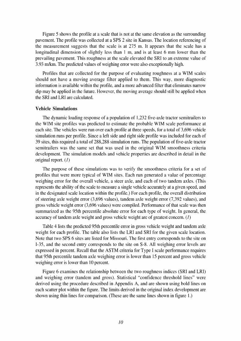
Figure 5 shows the profile at a scale that is not at the same elevation as the surrounding pavement. The profile was collected at a SPS 2 site in Kansas. The location referencing of the measurement suggests that the scale is at 275 m. It appears that the scale has a longitudinal dimension of slightly less than 1 m, and is at least 6 mm lower than the prevailing pavement. This roughness at the scale elevated the SRI to an extreme value of 3.93 d k m . The predicted values of weighing error were also exceptionally high.

Profiles that are collected for the purpose of evaluating roughness at a WIM scales should not have a moving average filter applied to them. This way, more diagnostic information is available within the profile, and a more advanced filter that eliminates narrow dip may be applied in the future. However, the moving average should still be applied when the SRI and LRI are calculated.

Vehicle Simulations

The dynamic loading response of a population of 1,232 five-axle tractor semitrailers to the WIM site profiles was predicted to estimate the probable WIM scale performance at each site. The vehicles were run over each profile at three speeds, for a total of 3,696 vehicle simulation runs per profile. Since a left side and right side profile was included for each of 39 sites, this required a total of 288,288 simulation runs. The population of five-axle tractor semitrailers was the same set that was used in the original WIM smoothness criteria development. The simulation models and vehicle properties are described in detail in the original report. ( I )

The purpose of these simulations was to verify the smoothness criteria for a set of profiles that were more typical of WIM sites. Each run generated a value of percentage weighing error for the overall vehicle, a steer axle, and each of two tandem axles. (This represents the ability of the scale to measure a single vehicle accurately at a given speed, and in the designated scale location within the profile.) For each profile, the overall distribution of steering axle weight error (3,696 values), tandem axle weight error (7,392 values), and gross vehicle weight error (3,696 values) were compiled. Performance of that scale was then summarized as the 95th percentile absolute error for each type of weight. In general, the accuracy of tandem axle weight and gross vehicle weight are of greatest concern. ( I )

Table 4 lists the predicted 95th percentile error in gross vehicle weight and tandem axle weight for each profile. The table also lists the LRI and SRI for the given scale location. Note that two SPS 6 sites are listed for Missouri. The first entry corresponds to the site on 1-35, and the second entry corresponds to the site on S-8. All weighing error levels are expressed in percent. Recall that the ASTM criteria for Type I scale performance requires that 95th percentile tandem axle weighing error is lower than 15 percent and gross vehicle weighing error is lower than 10 percent.

Figure 6 examines the relationship between the two roughness indices (SRI and LRI) and weighing error (tandem and gross). Statistical "confidence threshold lines" were derived using the procedure described in Appendix A, and are shown using bold lines on each scatter plot within the figure. The limits derived in the original index development are shown using thin lines for comparison. (These are the same lines shown in figure 1 .)

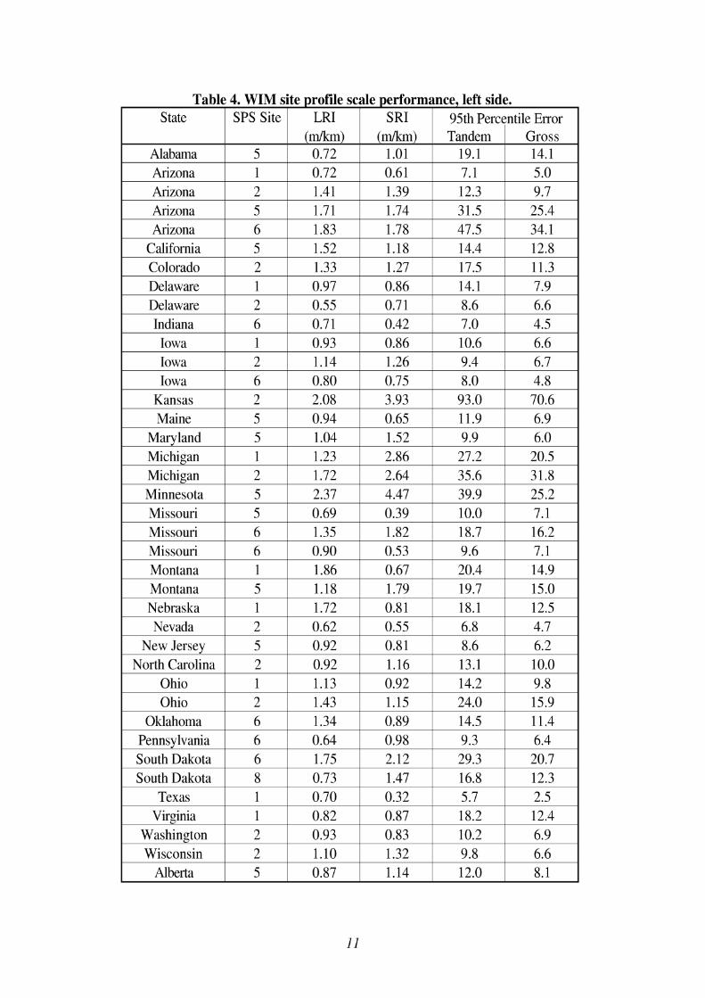
Table 4. WIM site profile scale performance, left side.

Arizona 2 1.41 1.39 12.3 9.7 1

State SPS Site ~ LRI

Alabama Arizona

SRI 95th Percentile Error

California 5 1.52 1.18 14.4 12.8 1

5 1

Arizona Arizona

Delaware 2 0.55 0.71 8.6 6.6 1

(m/km) 0.72 0.72

5 6

Colorado Delaware

Iowa 1 2 1.14 1.26 9.4 6.7 1

(m/km) 1.01 0.61

1.71 1.83

2 1

Indiana Iowa

Tandem 19.1 7.1

1.74 1.78

1.33 0.97

6 1

Iowa

Marvland 5 1.04 1.52 9.9 6.0 1

Gross 14.1 5.0

Kansas Maine

3 1.5 47.5

1.27 0.86

0.71 0.93

6

Minnesota 5 2.37 4.47 39.9 25.2 1

25.4 34.1

2 5

Michigan Michigan

17.5 14.1

0.42 0.86

0.80

Missouri 6 0.90 0.53 9.6 7.1 1

11.3 7.9

2.08 0.94

1 2

Missouri Missouri

7.0 10.6

0.75

Montana 5 1.18 1.79 19.7 15.0 1

4.5 6.6

3.93 0.65

1.23 1.72

5 6

Montana

Nebraska 1 1.72 0.81 18.1 12.5 1

8.0

Nevada 2 0.62 0.55 6.8 4.7 1

4.8 93.0 11.9

2.86 2.64

0.69 1.35

1

70.6 6.9

Ohio 1 1 1.13 0.92 14.2 9.8 1

27.2 35.6

0.39 1.82

1.86

New Jersey North Carolina

20.5 31.8

Pennsvlvania 6 0.64 0.98 9.3 6.4 1

10.0 18.7

0.67

5 2

Ohio Oklahoma

7.1 16.2

Texas 1 1 0.70 0.32 5.7 2.5 1

20.4

0.92 0.92

2 6

South Dakota South Dakota

14.9

0.81 1.16

1.43 1.34

6 8

Virginia

Wisconsin 2 1.10 1.32 9.8 6.6 1 Washington ~ 2

8.6 13.1

1.15 0.89

1.75 0.73

1

6.2 10.0

0.93

Alberta

24.0 14.5

2.12 1.47

0.82

15.9 11.4

0.83

5

29.3 16.8

0.87

20.7 12.3

10.2

0.87

18.2 6.9 12.4

1.14 12.0 8.1

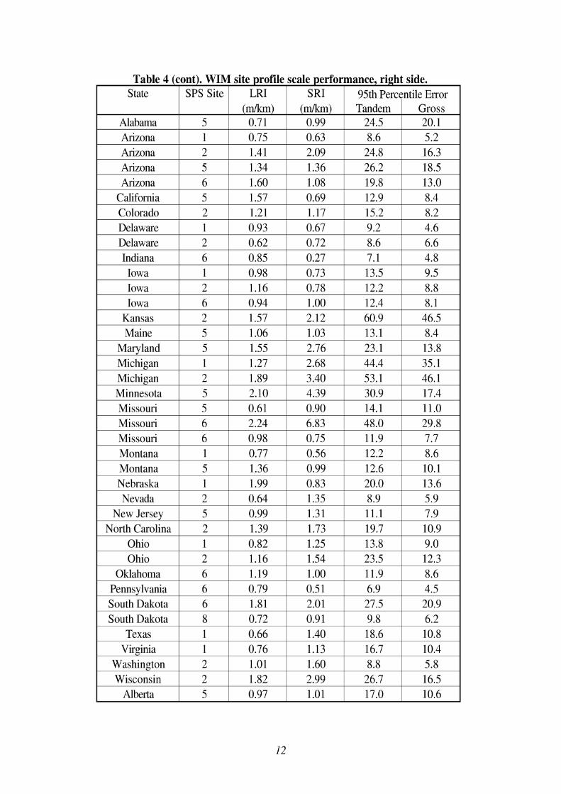
Table 4 (cont). WIM site profile scale performance, right side.

Arizona 2 1.41 2.09 24.8 16.3 1

State SPS Site ~ LRI

Alabama Arizona

SRI 95th Percentile Error

California 5 1.57 0.69 12.9 8.4 1

5 1

Arizona Arizona

Delaware 2 0.62 0.72 8.6 6.6 1

(m/km) 0.71 0.75

5 6

Colorado Delaware

Iowa 1 2 1 . 1 6 0 . 7 8 1 2 . 2 8.8 1

(m/km) 0.99 0.63

1.34 1.60

2 1

Indiana Iowa

Tandem 24.5 8.6

1.36 1.08

1.21 0.93

6 1

Iowa

Marvland 5 1.55 2.76 23.1 13.8 1

Gross 20.1 5.2

Kansas Maine

26.2 19.8

1.17 0.67

0.85 0.98

6

Minnesota 5 2.10 4.39 30.9 17.4 1

18.5 13 .O

2 5

Michigan Michigan

15.2 9.2

0.27 0.73

0.94

Missouri 6 0.98 0.75 11.9 7.7 1

8.2 4.6

1.57 1.06

1 2

Missouri Missouri

7.1 13.5

1 .OO

Nebraska 1 1.99 0.83 20.0 13.6 1

4.8 9.5

2.12 1.03

1.27 1.89

5 6

Montana Montana

Nevada 2 0.64 1.35 8.9 5.9 1

12.4 8.1 60.9 13.1

2.68 3.40

0.61 2.24

1 5

Ohio 1 1 0.82 1.25 13.8 9.0 1

46.5 8.4

New Jersey North Carolina

44.4 53.1

0.90 6.83

0.77 1.36

Pennsvlvania 6 0.79 0.51 6.9 4.5 1

35.1 46.1

5 2

Ohio Oklahoma

14.1 48.0

0.56 0.99

Texas 1 1 0.66 1.40 18.6 10.8 1

11.0 29.8

0.99 1.39

2 6

South Dakota South Dakota

12.2 12.6

Washington 2 1.01 1.60 8.8 5.8 1

8.6 10.1

1.31 1.73

1.16 1.19

6 8

Virginia

Wisconsin 2 1.82 2.99 26.7 16.5 1

11.1 19.7

1.54 1 .OO

1.81 0.72

1

7.9 10.9

Alberta

23.5 11.9

2.01 0.91

0.76

12.3 8.6

5

27.5 9.8

1.13

20.9 6.2

0.97

16.7 10.4

1.01 17.0 10.6

95 Percentile Tandem Axle Error 95 100 1

Percentile Gross Weight Error 80 1

0.0 .5 1.0 1.5 2.0 2.5 0.0 .5 1.0 1.5 2.0 2.5 LRI ( d k m ) LRI ( d m )

95 Percentile Tandem Axle Error 95 Percentile Gross Weight Error 100

90

80

70

60

5 0

40

3 0

20

10

0 0 1 2 3 4 5 6 7 0 1 2 3 4 5 6 7

SRI ( d k m ) SRI (mlkm)

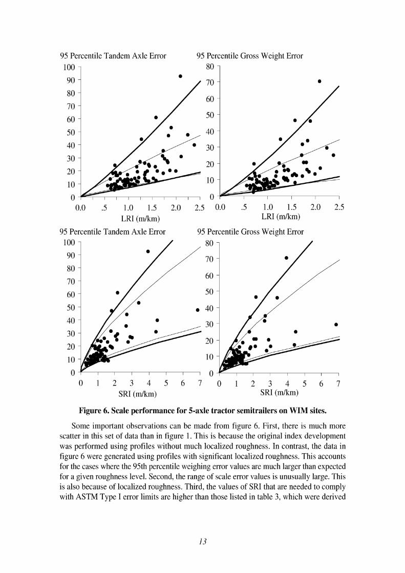
Figure 6. Scale performance for 5-axle tractor semitrailers on WIM sites.

Some important observations can be made from figure 6. First, there is much more scatter in this set of data than in figure 1. This is because the original index development was performed using profiles without much localized roughness. In contrast, the data in figure 6 were generated using profiles with significant localized roughness. This accounts for the cases where the 95th percentile weighing error values are much larger than expected for a given roughness level. Second, the range of scale error values is unusually large. This is also because of localized roughness. Third, the values of SRI that are needed to comply with ASTM Type I error limits are higher than those listed in table 3, which were derived

using a different set of profiles. (Recall that the ASTM limits are 15 percent for tandem axles and 10 percent for gross vehicle weight.)

Table 5 lists the roughness index thresholds that would be appropriate for the data in figure 6. For each index, the suggested threshold values should be the lowest among the two types of scale error. (For example, the value of 2.09 m/km would take priority over 2.20 mlkm for LRI, so that both types of scale reading would meet the necessary requirements.) Thus, the lower threshold for LRI would be about 0.5 m/km, and the upper threshold would be about 2.1 m/km. Recall that the lower threshold virtually guarantees acceptable scale performance and the upper threshold virtually guarantees unacceptable scale performance. These limits on LRI are very similar to the limits that were derived using data from the original index development. (See table 3.)

Table 5. Roughness Index Thresholds, WIM Site Profiles. Index WIM Error Type Lower Threshold Upper Threshold

(h) (mb) LRI Tandem Axle Load 0.53 2.09 LRI Gross Weight 0.51 2.20 SRI Tandem Axle Load 0.43 2.70 SRI Gross Weight 0.39 2.86

The lower threshold for SRI indicated by this data set is about 0.4 rnlkm and the upper threshold is 2.7 mlkm. This upper threshold is quite different than the one suggested in table 3. This is because the data set used to derive table 5 included significant localized roughness, and the data set used to derive table 3 did not. Primarily, this is because localized roughness that is just outside of the range of the SRI elevated the simulated WIM error level severely in some cases without a commensurate impact on the SRI. This is depicted by some very high values in figure 6 that are not very far to the right.

To help correct this, and to tighten up the correlation between SRI and predicted scale error, the SRI needs to be altered to include a wider range of pavement near the scale. However, changing the weighting function width of 3.2 m would alter the meaning of the index. Thus, this was done by replacing the SRI for a specific location with the maximum value that occurs for a range near the scale. A search for the optimal range was performed that would minimize the residuals for the correlation between scale error and SRI, using a logarithmic model. (This model, and the way residuals are used is described in Appendix A,) Note that the residuals determine the separation between the boundaries of the "confidence curves" shown in figure 6. The optimal range was found to be 2.45 m ahead of the scale through 1.5 m behind the scale. (Do not confuse this with the spatial weighting function limits of 2.74 m ahead of a point of interest through 0.46 m afterward. These are not altered.)

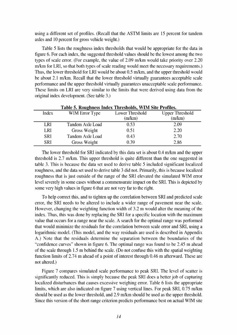
Figure 7 compares simulated scale performance to peak SRI. The level of scatter is significantly reduced. This is simply because the peak SRI does a better job of capturing localized disturbances that causes excessive weighing error. Table 6 lists the appropriate limits, which are also indicated on figure 7 using vertical lines. For peak SRI, 0.75 m/km should be used as the lower threshold, and 2.9 m/km should be used as the upper threshold. Since this version of the short range criterion predicts performance best on actual WIM site

profiles, it is recommended as a replacement to the original criterion. (This is really the original criterion, with a simple step added to it.)

95 Percentile Tandem Axle Error 95 Percentile Gross Weight Error

0 1 2 3 4 5 6 7 8 0 1 2 3 4 5 6 7 8 Peak SRI (dk rn ) Peak SRI (mtkm)

Figure 7. Scale performance compared to peak SRI.

Table 6. Roughness Index Thresholds, WIM Site Profiles. Index WIM Error Type Lower Threshold Upper Threshold - A A A

( h ) ( h ) Peak SRI Tandem Axle Load 0.82 2.90 Peak SRI Gross Weight 0.75 3.04

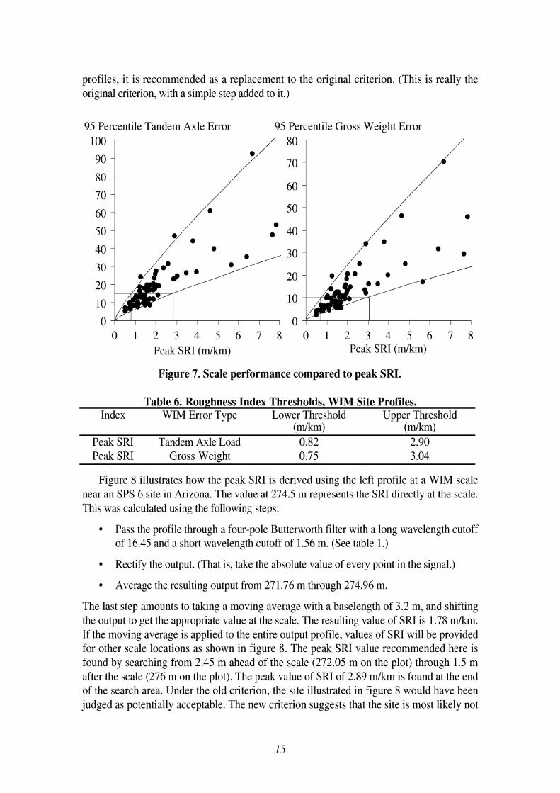
Figure 8 illustrates how the peak SRI is derived using the left profile at a WIM scale near an SPS 6 site in Arizona. The value at 274.5 m represents the SRI directly at the scale. This was calculated using the following steps:

Pass the profile through a four-pole Butterworth filter with a long wavelength cutoff of 16.45 and a short wavelength cutoff of 1.56 m. (See table I.)

Rectify the output. (That is, take the absolute value of every point in the signal.)

Average the resulting output from 271 -76 m through 274.96 m.

The last step amounts to taking a moving average with a baselength of 3.2 m, and shifting the output to get the appropriate value at the scale. The resulting value of SRI is 1.78 d k m . If the moving average is applied to the entire output profile, values of SRI will be provided for other scale locations as shown in figure 8. The peak SRI value recommended here is found by searching from 2.45 m ahead of the scale (272.05 m on the plot) through 1.5 m after the scale (276 m on the plot). The peak value of SRI of 2.89 m/km is found at the end of the search area. Under the old criterion, the site illustrated in figure 8 would have been judged as potentially acceptable. The new criterion suggests that the site is most likely not

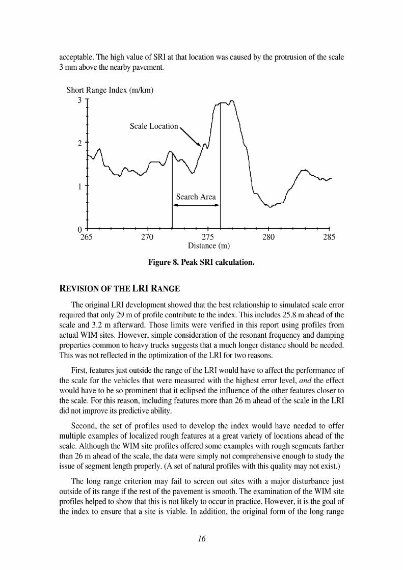
acceptable. The high value of SRI at that location was caused by the protrusion of the scale 3 mm above the nearby pavement.

Short Range Index (dkm)

I - - - - , - - - - I

265 270 275 280 Distance (m)

Figure 8. Peak SRI calculation.

REVISION OF THE LRI RANGE

The original LRI development showed that the best relationship to simulated scale error required that only 29 m of profile contribute to the index. This includes 25.8 m ahead of the scale and 3.2 m afterward. Those limits were verified in this report using profiles from actual WIM sites. However, simple consideration of the resonant frequency and damping properties common to heavy trucks suggests that a much longer distance should be needed. This was not reflected in the optimization of the LRI for two reasons.

First, features just outside the range of the LRI would have to affect the performance of the scale for the vehicles that were measured with the highest error level, and the effect would have to be so prominent that it eclipsed the influence of the other features closer to the scale. For this reason, including features more than 26 m ahead of the scale in the LRI did not improve its predictive ability.

Second, the set of profiles used to develop the index would have needed to offer multiple examples of localized rough features at a great variety of locations ahead of the scale. Although the WIM site profiles offered some examples with rough segments farther than 26 m ahead of the scale, the data were simply not comprehensive enough to study the issue of segment length properly. (A set of natural profiles with this quality may not exist.)

The long range criterion may fail to screen out sites with a major disturbance just outside of its range if the rest of the pavement is smooth. The examination of the WIM site profiles helped to show that this is not likely to occur in practice. However, it is the goal of the index to ensure that a site is viable. In addition, the original form of the long range

criterion may create the false impression that only 26 m of pavement must be resurfaced or rehabilitated to create an acceptable WIM site. This could have disastrous results if the rough transition between pavement types is placed only slightly more than 26 m ahead of a scale.

To help study the sensitivity of scale performance to rough profile features, three artificial profile "disturbances" were examined:

1. Cleat: This is a very narrow, upward spike in the profile.

2. Step: This is a step change in elevation. Examples of upward and downward steps were examined.

3. Slope Break: This is a sudden change in grade.

These represent elevation, slope. and curvature impulses, respectively. Each type of disturbance was studied with perfectly smooth profile surrounding it. The response of the population of five-axle tractor semitrailers to each feature was calculated. The sensitivity of the vehicles to these disturbances were summarized by deriving the 95th percentile tandem axle weighing error a multiple locations after they were encountered. The cleat was found to impact scale performance for only a short distance. For example, a cleat that was 50 mm high caused only a 2 percent scale error level when it was outside of the range of the LRI. This is because a cleat provides much more excitation to high frequency motion than to low frequency motion. The result is a high level of axle hop, but that damps out after a relatively short distance.

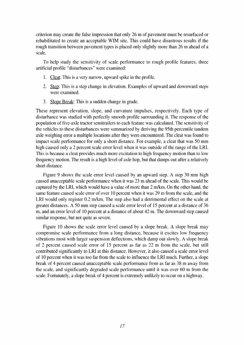
Figure 9 shows the scale error level caused by an upward step. A step 30 mm high caused unacceptable scale performance when it was 23 m ahead of the scale. This would be captured by the LRI, which would have a value of more than 2 mlkm. On the other hand, the same feature caused scale error of over 10 percent when it was 29 m from the scale, and the LRI would only register 0.2 mlkm. The step also had a detrimental effect on the scale at greater distances. A 50 mm step caused a scale error level of 15 percent at a distance of 36 m, and an error level of 10 percent at a distance of about 42 m. The downward step caused similar response, but not quite as severe.

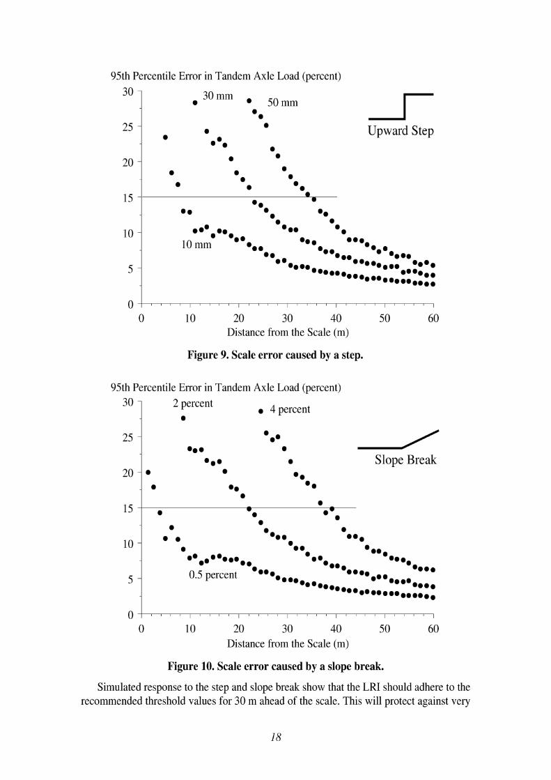
Figure 10 shows the scale error level caused by a slope break. A slope break may compromise scale performance from a long distance, because it excites low frequency vibrations most with larger suspension deflections, which damp out slowly. A slope break of 2 percent caused scale error of 15 percent as far as 22 m from the scale. but still contributed significantly to LRI at this distance. However, it also caused a scale error level of 10 percent when it was too far from the scale to influence the LRI much. Further, a slope break of 4 percent caused unacceptable scale performance from as far as 38 m away from the scale, and significantly degraded scale performance until it was over 60 m from the scale. Fortunately, a slope break of 4 percent is extremely unlikely to occur on a highway.

95th Percentile Error in Tandem Axle Load (percent)

Upward Step

0 ~ " " l " l " " l " " l " " l " " l

0 10 20 3 0 40 5 0 60 Distance from the Scale (m)

Figure 9. Scale error caused by a step.

95th Percentile Error in Tandem Axle Load (percent) 2 percent 4 percent

me* • Slope Break *.

*e a.

. e*e..*a..

0.5 percent ***ee **a

o ~ l l l l l l l 1 1 1 1 ' 1 1 1 1 1 1 1 1 1 1 1 1 1 1 1 1

0 10 20 3 0 40 5 0 60 Distance from the Scale (m)

Figure 10. Scale error caused by a slope break.

Simulated response to the step and slope break show that the LRI should adhere to the recommended threshold values for 30 m ahead of the scale. This will protect against very

rough features that are outside of the range of influence of the LRI for the precise scale location. This will also help motivate a more rational approach to corrective action, such as grinding, at WIM scale approaches. In addition, it may eliminate cases where the pavement is sufficient when the profiles are measured, but may deteriorate rapidly in the near future. The search area of 30 m is considered an absolute minimum. For example, when a plan for corrective action is developed for an existing WIM site, a search area of at least 30 m must be used. When the LRI is used to search a pavement for an ideal WIM scale location, a value of 30 m is required, but a value of 60 m is suggested.

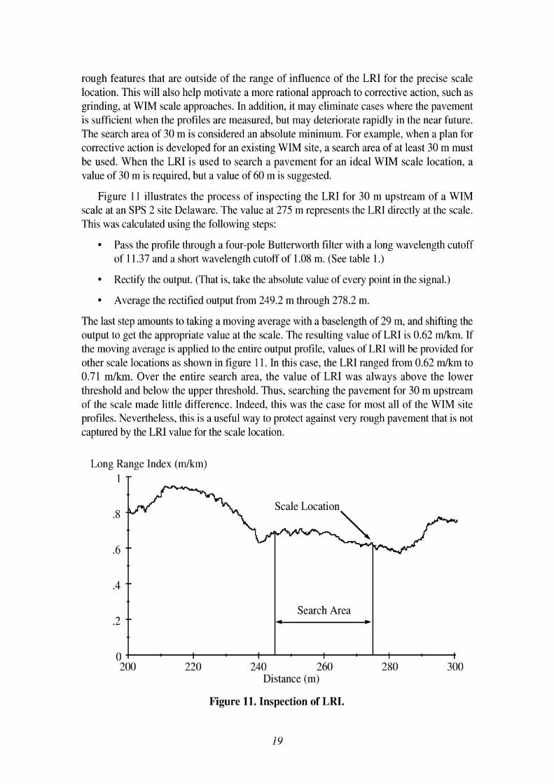
Figure 11 illustrates the process of inspecting the LRI for 30 m upstream of a WIM scale at an SPS 2 site Delaware. The value at 275 m represents the LRI directly at the scale. This was calculated using the following steps:

Pass the profile through a four-pole Butterwosth filter with a long wavelength cutoff of 11.37 and a short wavelength cutoff of 1.08 m. (See table 1.)

Rectify the output. (That is, take the absolute value of every point in the signal.)

Average the rectified output from 249.2 m through 278.2 m.

The last step amounts to taking a moving average with a baselength of 29 m, and shifting the output to get the appropriate value at the scale. The resulting value of LRI is 0.62 d k m . If the moving average is applied to the entire output profile, values of LRI will be provided for other scale locations as shown in figure 1 1. In this case, the LRI ranged from 0.62 d k m to 0.71 mlkm. Over the entire search area, the value of LRI was always above the lower threshold and below the upper threshold. Thus, searching the pavement for 30 m upstream of the scale made little difference. Indeed, this was the case for most all of the WIM site profiles. Nevertheless, this is a useful way to protect against very rough pavement that is not captured by the LRI value for the scale location.

Long Range Index ( d k m ) 1 T

200 220 240 260 280 300 Distance (m)

Figure 11. Inspection of LRI.

RECOMMENDATIONS

This research verified the SRI and LRI for predicting WIM scale error on five-axle tractor semitrailers and three-axle straight trucks. The research also verified them for a set of profiles collected at actual WIM sites. However, the research discovered that some enhancements in the way the indices are used would improve their ability to screen WIM sites for excessive road roughness.

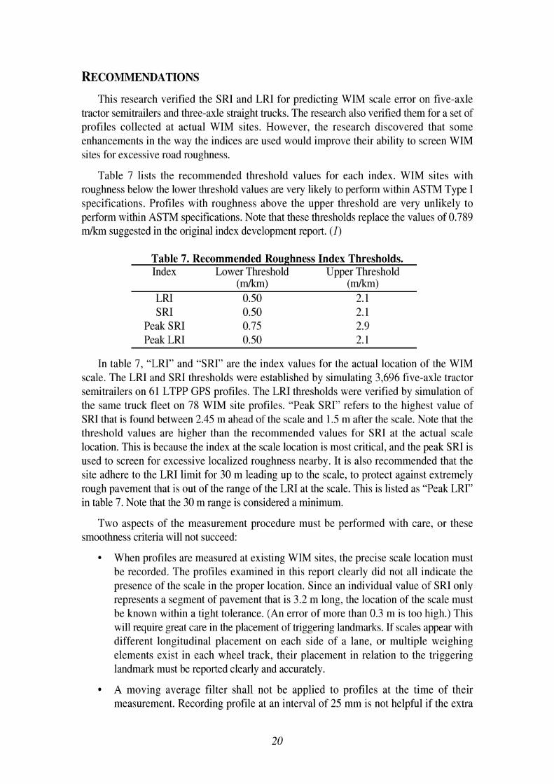
Table 7 lists the recommended threshold values for each index. WIM sites with roughness below the lower threshold values are very likely to perform within ASTM Type I specifications. Profiles with roughness above the upper threshold are very unlikely to perform within ASTM specifications. Note that these thresholds replace the values of 0.789 rntkrn suggested in the original index development report. ( I )

Table 7. Recommended Roughness Index Thresholds. Index Lower Threshold Upper Threshold

(h) (dkm) LRI 0.50 SRI 0.50

Peak SRI 0.75 Peak LRI 0.50

In table 7, "LRI" and "SRI" are the index values for the actual location of the WIM scale. The LRI and SRI thresholds were established by simulating 3,696 five-axle tractor semitrailers on 61 LTPP GPS profiles. The LRI thresholds were verified by simulation of the same truck fleet on 78 WIM site profiles. "Peak SRI" refers to the highest value of SRI that is found between 2.45 m ahead of the scale and 1.5 m after the scale. Note that the threshold values are higher than the recommended values for SRI at the actual scale location. This is because the index at the scale location is most critical, and the peak SRI is used to screen for excessive localized roughness nearby. It is also recommended that the site adhere to the LRI limit for 30 m leading up to the scale, to protect against extremely rough pavement that is out of the range of the LRI at the scale. This is listed as "Peak LRI'' in table 7. Note that the 30 m range is considered a minimum.

Two aspects of the measurement procedure must be performed with care, or these smoothness criteria will not succeed:

When profiles are measured at existing WIM sites, the precise scale location must be recorded. The profiles examined in this report clearly did not all indicate the presence of the scale in the proper location. Since an individual value of SRI only represents a segment of pavement that is 3.2 m long, the location of the scale must be known within a tight tolerance. (An error of more than 0.3 m is too high.) This will require great care in the placement of triggering landmarks. If scales appear with different longitudinal placement on each side of a lane, or multiple weighing elements exist in each wheel track, their placement in relation to the triggering landmark must be reported clearly and accurately.

A moving average filter shall not be applied to profiles at the time of their measurement. Recording profile at an interval of 25 mm is not helpful if the extra

information it would provide is eliminated by a 300 mm moving average. The moving average must remain a part of the procedure for calculating the SRI and LRI, but only as a post-processing step. Reporting profile without the moving average will allow further analysis of profiles with severe spikes near the scale in the future. In particular, it will permit the application of a replacement for the moving average with a more accurate representation of the way tires bridge over narrow dips.

The majority of WIM site profiles included localized roughness at the scale, which consistently impacted the LRI, the SRI, and the level of dynamic loading predicted by the vehicle simulations. Two types of roughness were common: (1) narrow, downward spikes that were most likely caused by surface scarring at the inductive loops or gaps between the scales and their housing, and (2) scales that were not at the same elevation as the surrounding pavement. Some of the profiles also had upward spikes without an obvious source. Agencies in charge of WIM scales should be encouraged to inspect their WIM site profiles for these features, and all candidate SPS traffic study site profiles should be carefully inspected. (The SRI will estimate the effect of localized scale roughness, but profile inspection is needed to find the cause.) Appendix B provides an example of this process for the WIM site profiles. This will help address obvious problems that may require more careful scale installation.

All of the findings presented in this report are the result of simulations. Validation is strongly recommended. It is not practical to perform tests over as diverse a range of trucks as were covered in the simulations. However, measurements of WIM scale error for a limited number of vehicles of known configuration and suspension properties may be performed. This would provide a basis for comparison to simulations of those vehicles over measure approach pavement profiles.

REFERENCES

1. Karamihas, S. M. and Gillespie, T. D.? "Smoothness Criteria for WIM Scale Approaches." University of Michigan Transportation Research Institute Report UMTRI-2002-37 (2002) 81 p.

2. Sayers, M. W, and Karamihas, S. M., "Interpretation of Road Roughness Profile Data.'' Federal Highway Administration Report FHWAIRD-961101 (1996) 177 p.

3. American Society of Testing and Materials, Annual Book of ASTM Standards, Volume 4.03, Road and Paving Materials; Vehicle-Pavement Systems, Philadelphia, 1999.

4. Massie, D. L. "Large-Truck Population Estimates Based on the 1987 Truck Inventory and Use Survey. Special Report." Great Lakes Center for Truck Transportation Research Report No. GLCTTR 04-92/11 UMTRI-92-5 (1992).

5. Long Term Pavement Performance Program Directive P-30, August 2003.

Appendix A: Index Threshold Development

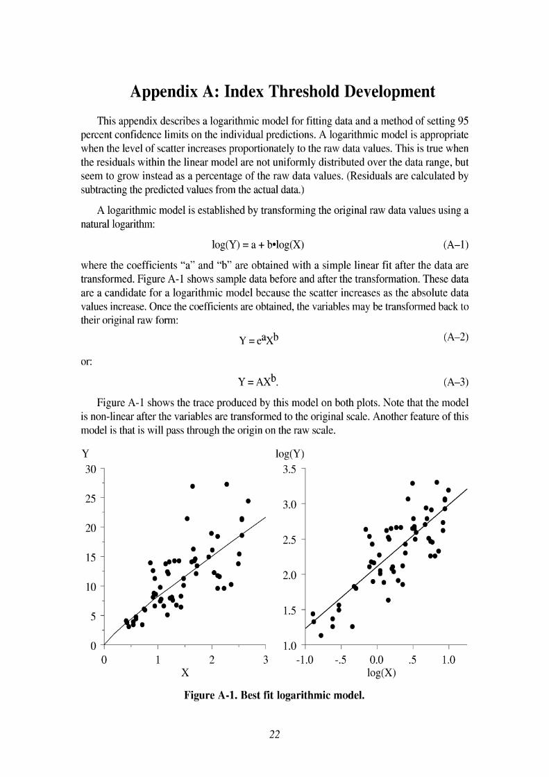
This appendix describes a logarithmic model for fitting data and a method of setting 95 percent confidence limits on the individual predictions. A logarithmic model is appropriate when the level of scatter increases proportionately to the raw data values. This is true when the residuals within the linear model are not uniformly distributed over the data range, but seem to grow instead as a percentage of the raw data values. (Residuals are calculated by subtracting the predicted values from the actual data.)

A logarithmic model is established by transforming the original raw data values using a natural logarithm:

where the coefficients "a" and "b" are obtained with a simple linear fit after the data are transformed. Figure A-1 shows sample data before and after the transformation. These data are a candidate for a logarithmic model because the scatter increases as the absolute data values increase. Once the coefficients are obtained, the variables may be transformed back to their original raw form:

Y = e a ~ b (A-2)

or:

Figure A-1 shows the trace produced by this model on both plots. Note that the model is non-linear after the variables are transformed to the original scale. Another feature of this model is that is will pass through the origin on the raw scale.

Figure A-1. Best fit logarithmic model.

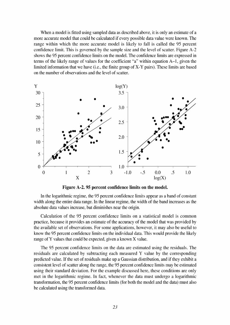
When a model is fitted using sampled data as described above, it is only an estimate of a more accurate model that could be calculated if every possible data value were known. The range within which the more accurate model is likely to fall is called the 95 percent confidence limit. This is governed by the sample size and the level of scatter. Figure A-2 shows the 95 percent confidence limits on the model. The confidence limits are expressed in terms of the likely range of values for the coefficient "a" within equation A-1, given the limited information that we have (i.e., the finite group of X-Y pairs). These limits are based on the number of observations and the level of scatter.

Figure A-2.95 percent confidence limits on the model.

In the logarithmic regime, the 95 percent confidence limits appear as a band of constant width along the entire data range. In the linear regime, the width of the band increases as the absolute data values increase, but diminishes near the origin.

Calculation of the 95 percent confidence limits on a statistical model is common practice, because it provides an estimate of the accuracy of the model that was provided by the available set of observations. For some applications, however, it may also be useful to know the 95 percent confidence limits on the individual data. This would provide the likely range of Y values that could be expected, given a known X value.

The 95 percent confidence limits on the data are estimated using the residuals. The residuals are calculated by subtracting each measured Y value by the corresponding predicted value. If the set of residuals make up a Gaussian distribution, and if they exhibit a consistent level of scatter along the range, the 95 percent confidence limits may be estimated using their standard deviation. For the example discussed here, these conditions are only met in the logarithmic regime. In fact, whenever the data must undergo a logarithmic transformation, the 95 percent confidence limits (for both the model and the data) must also be calculated using the transformed data.

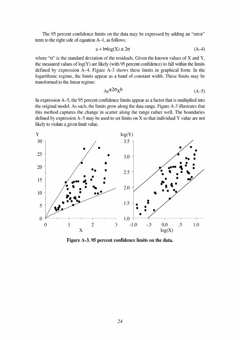
The 95 percent confidence limits on the data may be expressed by adding an "error" term to the right side of equation A-1, as follows:

where "o" is the standard deviation of the residuals. Given the known values of X and Y, the measured values of log(Y) are likely (with 95 percent confidence) to fall within the limits defined by expression A-4. Figure A-3 shows these limits in graphical form. In the logarithmic regime, the limits appear as a band of constant width. These limits may be transformed to the linear regime:

In expression A-5, the 95 percent confidence limits appear as a factor that is multiplied into the original model. As such, the limits grow along the data range. Figure A-3 illustrates that this method captures the change in scatter along the range rather well. The boundaries defined by expression A-5 may be used to set limits on X so that individual Y value are not likely to violate a given limit value.

Figure A-3.95 percent confidence limits on the data.

Appendix B: Road Profiles

This appendix describes the road profiles used as input to vehicle simulations for this research. The matrix of profiles from the original weigh in motion (WIM) simulation study are briefly described, then the profiles collected at WIM sites are described in detail.

SIMULATION MATRIX

A matrix of road profile measurements was extracted from the Long-Term Pavement Performance (LTPP) Study Database for the original WIM simulation study. The matrix covers four pavement construction types: asphalt concrete, jointed plain concrete, jointed reinforced concrete, and asphalt overlay on concrete. These profiles were measured on sites from General Pavement Studies 1, 3, 4, and 7, respectively. For each construction type, profiles were assembled that span as large a range of International Roughness Index (IRI) as possible, with uniform representation over the range. To accomplish this, target roughness levels in multiples of 0.16 d k r n were covered from 0.47 d k r n to 3.47 d k r n . Thus, the matrix consists of up to 20 profile measurements for each construction type. Profile data were selected using the following criteria:

Only profiles from the left wheel path were considered.

Profiles were selected with IRI values near multiples of 0.16 m/km.

Profiles were avoided if Evans found them to have measurement errors. ( I )

Sites were avoided if the progression of IRI values over time could not be justified by the reported construction and maintenance history. (2, 3)

No more than one profile was used from a given site.

Sites without concentrated roughness were favored.

Profiles were favored from groups of repeat measurements with IRI values that have a low standard deviation.

Profiles were favored that showed good subjective visual agreement with other repeat measurements. Agreement was confirmed objectively by cross-correlating IRI filter output. (4)

Sites were selected to be as geographically diverse as possible.

All of the profile measurements covered a length of 152.4 meters. All of the measurements were also collected at a sample interval of 25.4 mm, averaged with a 304.8- mm baselength, and decimated to an interval of 152.4 mm. Note that the entire roughness range could not be covered for each pavement type, because profiles often did not exist within the LTPP database at both extremes. Thus, the IRI ranged from 0.50 to 3.90 d k r n for asphalt concrete, 0.78 to 3.43 mlkm for jointed plain concrete, 1.09 to 3.17 m/km for jointed reinforced concrete, and 0.48 to 2.09 mlkm for asphalt overlay on concrete.

WIM SITE PROFILES

These data were collected at 40 WIM sites. At each site, profile was measured at least 15 times, according to directive P-30: 5 times with the profiler in the center of the lane, 5 times with the profiler shifted to the left, and 5 times with the profiler shifted to the right. (5) The profile measurements were triggered so that they are at least 305 m long, and the scale appears at a location near 275 m. Most of the profiles collected before September 2002 are exactly 305 m long. Profiles collected after September 2002 are typically longer, but are still lined up with the scale as described above. Note that the profiles are automatically triggered, so no synchronization was necessary.

Table B-1 lists the WIM sites. K.J. Law T-6600 profilers measured about half of these profiles. These profiles were stored at a sample interval of 25 mm. No moving average was applied to these profiles before they were stored. Thus, a 300 mm moving average was applied to them before they were entered into the vehicle simulations. This filter was needed as a crude representation of tire envelopment. The rest of the profiles were measured with ICC profilers. These profilers also stored data at a sample interval of 25 mm, but a moving average with a 300 mm baselength was applied first.

Application of a tire envelopment filter is an important part of producing valid predictions of truck dynamic loads. However, the moving average should not be applied at the time of the measurement. Instead, the profiles should be stored without the averaging. Then the moving average may be applied later to condition profiles for vehicle simulations. This way, more detail is present within the profile for study of localized roughness and diagnosis of measurement errors. In particular, narrow, downward spikes may be more easily eliminated if they are viewed without the averaging. In addition, the un-averaged profiles are still compatible with improved tire envelopment filters.

A single profile was selected from each site for input to vehicle simulations. In every case, a measurement from the center of the lane was selected. In the majority of cases, the first repeat was selected. However, if the first repeat was found to include spikes that did not appear in other measurements, it was excluded in favor of another measurement.

Many of the measurements included an event marker at the location of the WIM scale. These always appeared very close to 275 m into the profile. Others did not. In most of these cases, an event marker appears 305 m into the profile, which signifies the end of the segment. (The exceptions are the sections in Nevada and California.) When no event marker appeared at the scale, it was assumed to be exactly 275 m into the profile. Table B-2 lists the scale location that was associated with each profile.

Several of these profiles include localized roughness that is associated with the presence of the scale. The roughness has several causes: (1) downward spikes caused by narrow dips at triggering loops upstream of the sensor, (2) narrow dips at the sensor itself, (3) scale mounting "error" (i.e., the scale failing to be flush with the pavement), and (4) conventional localized pavement roughness. Unfortunately, a moving average does not properly represent tire envelopment for narrow, downward spikes. Thus, the predicted dynamic tire loads will be artificially high, as well as the roughness index values. This will impose an upward bias in roughness at some scales, and may compromise the relationship between simulated axle weight error and roughness.

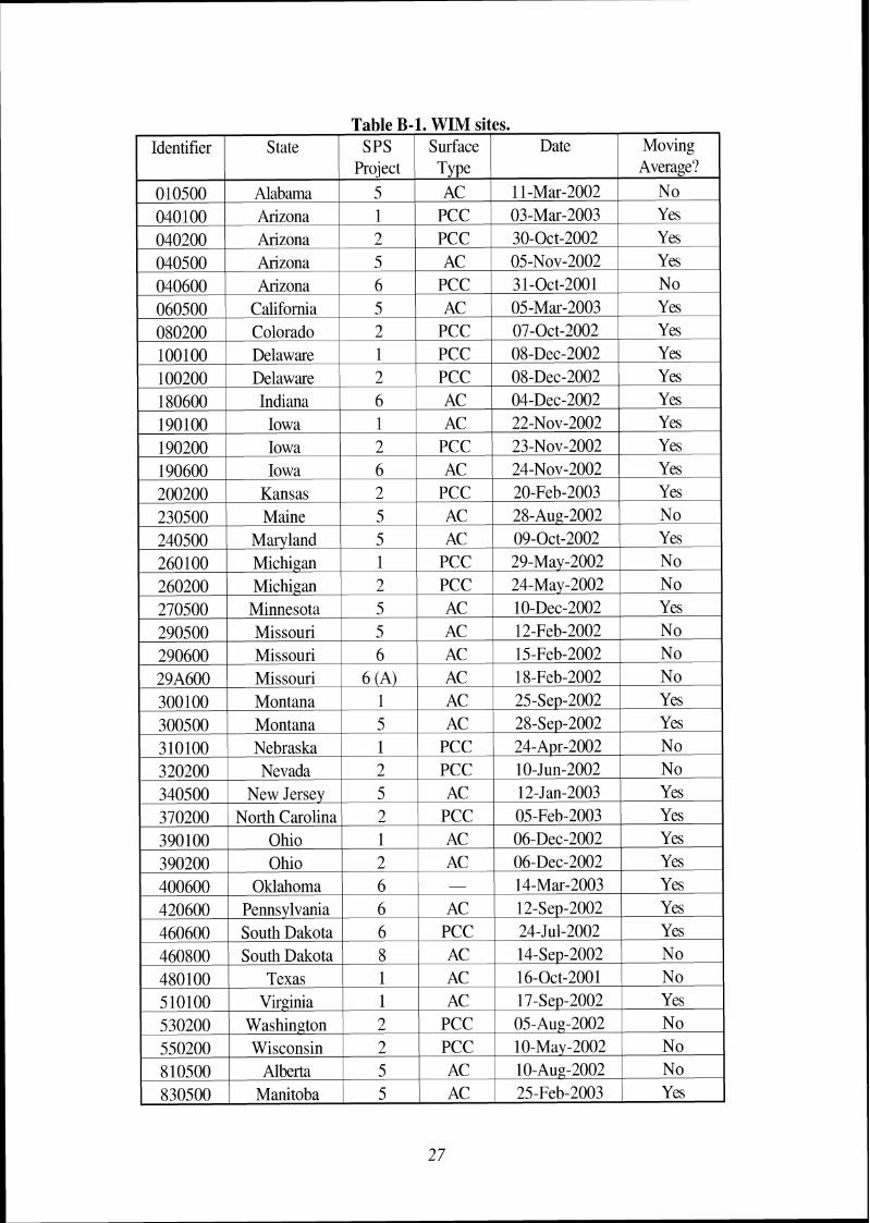
Table B-1. WIM sites. 1 Identifier I State 1 SPS 1 Surface 1 Date 1 Moving I

010500 040 100 040200 040500 040600 060500 080200 100100 100200 180600 190100 190200

Alabama

190600 200200

Arizona Arizona Arizona h z o n a

California Colorado Delaware Delaware Indiana

Iowa Iowa

550200 810500

1 830500

Proj ect 5

Iowa Kansas

1 2 5 6 5 2 1 2 6 1 2

Wisconsin Alberta

Manitoba

Type AC

6 2

PCC PCC AC

PCC AC

PCC PCC PCC AC AC

PCC

2 5 5

1 1-Mx-2002

AC PCC

Average? No

03-Mx-2003 30-Oct-2002 05-Nov-2002 3 1-Oct-2001 05-Mx-2003 07-Oct-2002 08-Dec-2002 08-Dec-2002 04-Dec-2002 22-Nov-2002 23-Nov-2002

PCC AC AC

Yes Yes Yes No Yes Yes Yes Yes Yes Yes Yes

24-Nov-2002 20-Feb-2003

Yes Yes

10-May-2002 10-Aug-2002 25-Feb-2003

No No Yes

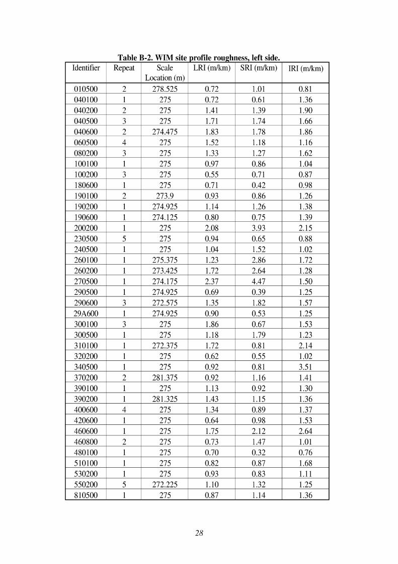
Table B-2. WIM site profile roughness, left side. I Identifier Repeat ~ Scale LRI (mikm) SRI (mikm) IRI (rnkm) I

010500 2 Location (m)

278.525 0.72 1.01 0.81

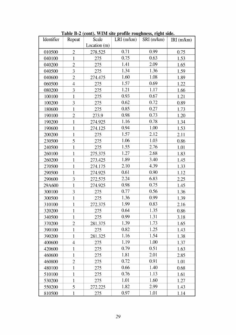
Table B-2 (cont). WIM site profile roughness, right side. I Identifier Repeat ~ Scale LRI (mikm) SRI (*) IRI (mkm) I

010500 040 100 040200 040500 040600 060500

2 1 2 3 2 4

Location (m) 278.525

275 275 275

274.475 275

0.71 0.75 1.41 1.34 1.60 1.57

0.99 0.63 2.09 1.36 1.08 0.69

0.75 1.53 1.65 1.59 1.89 1.22

Table B-2 provides the Long Range Index (LRI) and Short Range Index (SRI) for the listed scale location in each profile that was selected for simulation. The table also provides the IRI of the profiles from 155 m to 305 m into the segment. Section 830500 is not listed, because the run was terminated before the scale was reached. Special observations about each set of profiles are listed here, because they may help explain elevated roughness values, and unusual simulation results. Note that 22 of the 39 segments have obvious localized roughness at or near the WIM scale. In many cases the roughness is genuine, but in some cases the roughness is caused by narrow, downward spikes that a vehicle tire would bridge over.

010500: This site has localized roughness at the scale. Spikes appear in all repeats. They are the least severe in repeat 2. A downward spike appears in the profile at 278.4 m that is 112 mm deep on the left side and 6 mm deep on the right side. Spikes appear in most of the repeats at about 60 m and 230 m. These may be caused by pavement markings at the ends of a conventional test section near the scale.

040100: A rough patch appears from 60 m to 80 m, including a rise and fall in elevation of 35 mm over the 20 m. (This is most likely at a transition from asphalt to concrete within the section.) There is lesser agreement between repeat measurements near the scale.

040200: Some of the measurements show drift relative to the others early in the segment. The first half of this segment has significant upward curl, with slab lengths that vary from 3.5 m to 4.6 m.

040500: There is clear evidence in the profile that the section has transverse cracking. Although the averaging make this less visible, many of the cracks have narrow downward spikes. The joints do not have a consistent spacing. A dip appears at 275 m in the left profile that is about 0.5 m wide and 4 mm deep. Four dips appear in the right profile between 270 m and 275 m.

040600: The second half of the profile, including the vicinity of the scale, has narrow downward spikes 2-5 mm deep every 4.6 m (approximately). There is not strong evidence of slab curling. On the left side, the profile is elevated about 3 mm between 274 m and 275 m. On the right side, this is preceded by a narrow dip 5 mm deep.

060500: A sharp spike 6 mm high is followed directly by a sharp dip 6 mm high at 260 m in the profiles of both sides. A dip appears in the right profile that is 1 m wide and 8 mm deep at 42 m. A similar, but less severe, dip appears in some repeats at 73 m.

080200: Downward spikes appear in the profiles at 238 m and 256 m in all of the repeats. They are the least severe in repeat 3.

100100: Some of the measurements show drift relative to the others early in the segment. The right side shows a 10 mm drop in 1 m of profile at 228 m. It is not as severe on the left side.

100200: There is obvious upward curl in the first half of the segment. The slabs are 6.1 m long. The performance of this site probably changes throughout the day.

180600: This profile has a large triangular bump on both sides that is 20 mm high and 2 m wide, centered at 57 m. Large dips, 0.3 m wide and 12 mm deep, appear at 278.3 m and 280.5 m in the right profile.

190100: There are multiple (genuine) narrow bumps and dips in this profile. None of them appear at the scale.

190200: This site has significant upward curl. The slabs are 4.6 m long.

190600: Multiple narrow dips appear in the first 200 m of this segment.

200200: Comparison to the measurements from April 2002 showed that the longitudinal distance referencing in the February 2003 measurement was incorrect, such that the scale was actually at 0 m. The profile was shifted to correct this. On both sides, the scale is 6-8 mm beneath the prevailing profile elevation. This caused a dip that is about 0.8 m wide, at least 6 mm deep, and flat in the center.

230500: This segment has a negative swell 3 m wide and 8 mm deep centered at 265 m. The left side profile has a spike at 273 m.

240500: Narrow dips appear in the right side profile at 251 m, 256 m, and 273 m. They are about 5 mm deep.

260100: A segment within this profile from 274.5 m to 278.5 m is elevated more than 5 mm from the surrounding pavement. A narrow dip also appears at 278.5 m that is about 10 mm deep on the left side and 5 mm deep on the right side.

260200: Narrow, shallow dips (about 1-2 mm deep) appear throughout the left and right side profiles with a spacing of 4.6 m. A severe dip appears from 272 m to 275 m. It is more than 15 mm deep, and has a narrow dip at the leading and trailing end.

270500: This segment is roughest, by far, from 230 m to 290 m. The scale appears to be elevated about 5 mm compared to the surrounding profile at the scale on the left side.

290500: Repeat numbers 2 and 3 have large downward spikes on the right side. No localized roughness was detected in the vicinity of the scale.

290600: This segment has extreme roughness at the scale on the right side. Further, the repeat measurements do not agree well on the shape of the disturbances. The profile has a wide dip from 268 m to 271 m, then another from 276.5 m to 279 m. Each dip about 15 mm deep, and flat in the center. (In other words, there is a downward fault on the leading end, and an upward step on the trailing end.) Both dips have very narrow dips at either end. On the left side, narrow dips (3-5 mm deep) appear at 268.8 m, 270.6 m, 276.6 m, and 278.6 m. Narrow upward spikes (2 mm high) appear on the left and right side at 272.4 m and 274.4 m.

29A600: This segment has no obvious localized roughness at the scale.

300100: A narrow dip appears in all repeat measurements on the right side except number 3. Narrow dips more than 3 mm deep appear in the right side profile at 13 1

m, 142 m, 158 m, 233 m, 237 m, 253 m, 265 m, and 269 m, and in the left side profile at 158 m.

300500: Repeat measurements do not agree well on the shape of the localized roughness near the scale. A narrow dip about 3 mm deep appears in the left profile at 276 m and 289.5 m.

310100: This segment has concrete that is curled upward with some faulting. The slabs are 5 m long. A severely tilted slab appears from 231 m to 237 m, with a 7 mm fault at the leading edge and a 4 mm fault at the trailing edge. Some of the more aggressive faulting appears from 250 m through 280 m (near the scale). The profile also contains a 4-mm drop-off at 272.4 m, followed by a 4-6 mm upward step at 274.6 m, followed by a 4-6 mm drop-off at 275.4 m.

320200: The segment is jointed concrete with upward curling and a joint spacing of 4.6 m. The performance of the scale may change throughout the day. A dip 0.6 m wide and 2 mm deep appears from 277.4 m to 278 m of the left side. A bump 0.8 m wide and 3 mm high appears from 272.4 m to 273.2 m on the right side.

340500: This segment is extremely rough from 150 m through 220 m.

370200: A huge spike appears on the right profile of repeat 1 at 270 m.

390100: Dips 2 mm deep appear near 275 m on both sides. On the right side, a triangular dip 5 m wide and 10 mm deep appears centered at 216 m. A dip appears on both sides at 233 m that is more than 15 mm deep.

390200: Repeat 5 is not synchronized with the others, and repeat 2 terminated too early. Upward curling is evident throughout the site. The slab length is 4.6 m. A dip appears in the left side profile from 281.4 m to 282.4 m that is about 3 mm deep, and on the right side from 280.2 m to 218.2 m that is about 4 mm deep.

400600: Repeats 2 and 3 are not synchronized with 4, 5, and 6. All of these measurements were stored without a high-pass filter applied to them. The level of drift in the profiles would have confounded the simulation, so a 91.4-m high-pass filter was applied. A 0.5-m wide dip appears on both sides. It is 6 mm deep on the left and 14 mm deep on the right. Dips also appear on both sides at 276 m (3-5 mm deep) and 280 m (1.5 mm deep).

420600: Repeat measurements agree well. No localized roughness was detected near the scale.

460600: The first half of this segment is an extreme case of faulting and slab tilt. Faults are 5-10 mm high. The spacing between faults varies from 4 to 7 m. The right side has three deep narrow dips: 40 mm deep at 82 m, 30 mm deep at 134 m, and 20 mm deep at 173.5 m.

460800: A dip 0.4 m wide and 6 mm deep appears in the right profile at 246.5 m. A narrow dip 5 mm deep appears on both sides between 272 m and 273 m.

480100: A dip 2 m wide and 10 mm deep appears from 108 m to 110 m on both sides. A dip appears in the right side at 273 m that is 0.6 m wide and 2 mm deep, and on

the left side at 278 m that is 0.5 m wide and 3 mm deep. A spike appears in the left profile at 278.5 m that is 4 mm high.

510100: No obvious localized roughness found near the scale.

530200: Upward spikes about 2 mm high appear on both sides at 272 m and 277 m.

550200: Downward spikes at joints and evidence of faulting appear throughout the profile. Severe roughness appears near the scale, including swells that are 2 m wide and 4-6 mm high near 274.5 m on the right side and 277 m on the left side.

810500: A narrow dip 8 mm deep appears near 12 m on both sides. Both sides also have a 6 mm downward step at 216.5 m. (This is most likely the result of the end of a chip seal leading into the section.) Three dips appear on the left side from 272 m to 276 m (2 mm deep). A dip 3 mm deep appears on the right side at 270 m.

830500: These profiles appear to have terminated before the scale was reached. Thus, this site was eliminated from the analysis.

REFERENCES

1. Evans, L. D, and Eltahan, A., "LTPP Profile Variability." Federal Highway Administration Report FHWA-RD-00-113 (2000) 178 p.

2. Datapave, Release 3.0, <http://www.tfhrc.gov/pavement/ltpp/datapave.htm>

3. Perera, R. W., et. al., "Investigation of the Development of Pavement Roughness." Federal Highway Administration Report FHWA-RD-97-147 (1998) 244 p.

4. Sayers, M. W, and Karamihas, S. M., "Interpretation of Road Roughness Profile Data." Federal Highway Administration Report FHWAIRD-961101 (1996) 177 p.

5. Long Term Pavement Performance Program Directive P-30, August 2003.

Appendix C: Simulation Models

This appendix provides a description of the simulation models used to predict the vertical wheel loads imposed on the pavement by virtual trucks running on measured profiles. This study examined three-axle straight trucks with common suspension configurations. The study was also confined to rigid body models of behavior in the pitch plane. These models are defined by the inertial elements (parts with mass), compliant elements (tires and suspensions), and specific kinematics and compliance needed to capture relevant suspension behavior. Two multi-body models were needed for this study. One model was needed for vehicles with four-spring and air-suspended drive axles, and another was needed for vehicles with the less common walking-beam suspension. These models require a modest list of specific parameters to describe individual trucks. Thus, while only two models were needed for the study, hundreds of parameter combinations were used to represent the broad range of vehicles operating on U.S. highways.

Two-dimensional (pitch-plane) rigid-body models are the most common type used for predicting vertical wheel loads imposed by heavy vehicles. (1, 2) In most instances they have been found to be sufficient for prediction of vehicle wheel loads. (3) For this study, the equations of motion for the simulation models used were written using the AUTOSIMTM software package. AUTOSIM automatically generates efficient simulation programs for mechanical systems composed of multiple rigid bodies. (4, 5) In AUTOSIM, an engineer describes the vehicle system in terms of the rigid bodies, the manner in which they are connected, compliant elements (linear or non-linear) within the system, and disturbance inputs. AUTOSIM formulates the equations of motion symbolically, and then writes a file containing the source code for a FORTRAN or C program that can numerically integrate the equations of motion. When the program is compiled and executed, it produces ready-to- plot data files of time histories of output variables of interest, such as wheel loads. AUTOSIM has been used to generate models for similar studies in the past. (1, 6) As such, it contains specialized modeling options needed to properly represent vehicle dynamic behavior such as truck suspension system friction and tandem axle load sharing. (7, 8)

The assumptions made in modeling three-axle straight trucks for this study are described here. Much of the material used in the description is paraphrased from existing literature. (1, 9, 10) Some improvements to the models should be considered for use in future studies. In particular, a better representation of tire envelopment may be needed to simulate truck response over narrow, concave profile features such as wide expansion joints. This may be especially important if the roughness at a weigh-in-motion scale is included in the profile.

The pitch-plane model, illustrated in figure C-1, includes a sprung mass for the vehicle body and three unsprung masses (one for each axle). The sprung mass translates vertically and longitudinally, and rotates in pitch. Thus, the sprung mass has three degrees of freedom. Each unsprung mass translates vertically relative to the sprung mass. This adds

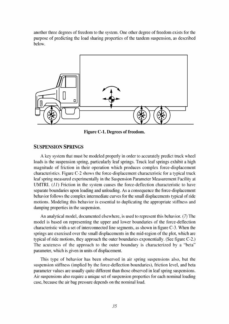
another three degrees of freedom to the system. One other degree of freedom exists for the purpose of predicting the load sharing properties of the tandem suspension, as described below.

Figure C-1. Degrees of freedom.

A key system that must be modeled properly in order to accurately predict truck wheel loads is the suspension spring, particularly leaf springs. Truck leaf springs exhibit a high magnitude of friction in their operation which produces complex force-displacement characteristics. Figure C-2 shows the force-displacement characteristic for a typical truck leaf spring measured experimentally in the Suspension Parameter Measurement Facility at UMTRI. (11) Friction in the system causes the force-deflection characteristic to have separate boundaries upon loading and unloading. As a consequence the force-displacement behavior follows the complex intermediate curves for the small displacements typical of ride motions. Modeling this behavior is essential to duplicating the appropriate stiffness and damping properties in the suspension.

An analytical model, documented elsewhere, is used to represent this behavior. (7) The model is based on representing the upper and lower boundaries of the force-deflection characteristic with a set of interconnected line segments, as shown in figure C-3. When the springs are exercised over the small displacements in the mid-region of the plot, which are typical of ride motions, they approach the outer boundaries exponentially. (See figure C-2.) The acuteness of the approach to the outer boundary is characterized by a "beta" parameter, which is given in units of displacement.

This type of behavior has been observed in air spring suspensions also, but the suspension stiffness (implied by the force-deflection boundaries), friction level, and beta parameter values are usually quite different than those observed in leaf spring suspensions. Air suspensions also require a unique set of suspension properties for each nominal loading case, because the air bag pressure depends on the nominal load.

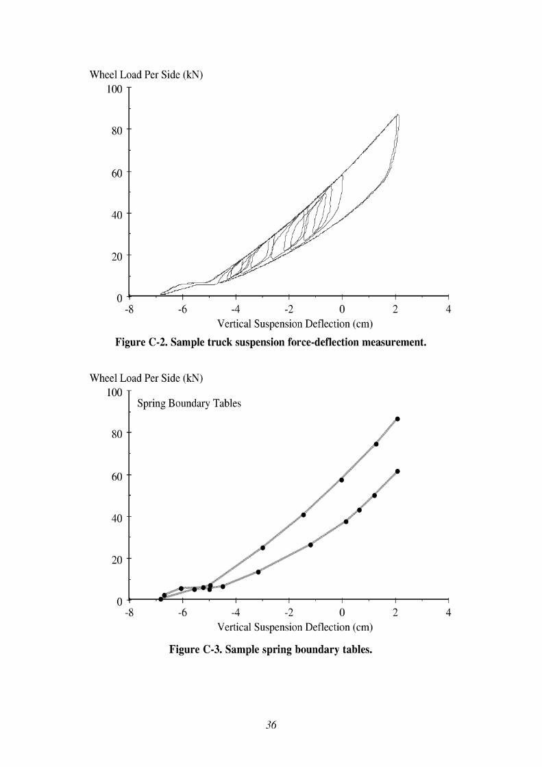
Wheel Load Per Side (kN)

loo T

- 8 -6 -4 -2 0 2 4 Vertical Suspension Deflection (cm)

Figure C-2. Sample truck suspension force-deflection measurement.

- 8 -6 -4 -2 0 2 4 Vertical Suspension Deflection (cm)

Wheel Load Per Side (kN)

Figure C-3. Sample spring boundary tables.

100

80

-

Spring Boundary Tables b

/\

-- I 4

@@ $#* 8

f 60 --

40 --

20 --

0 -' I I I I I

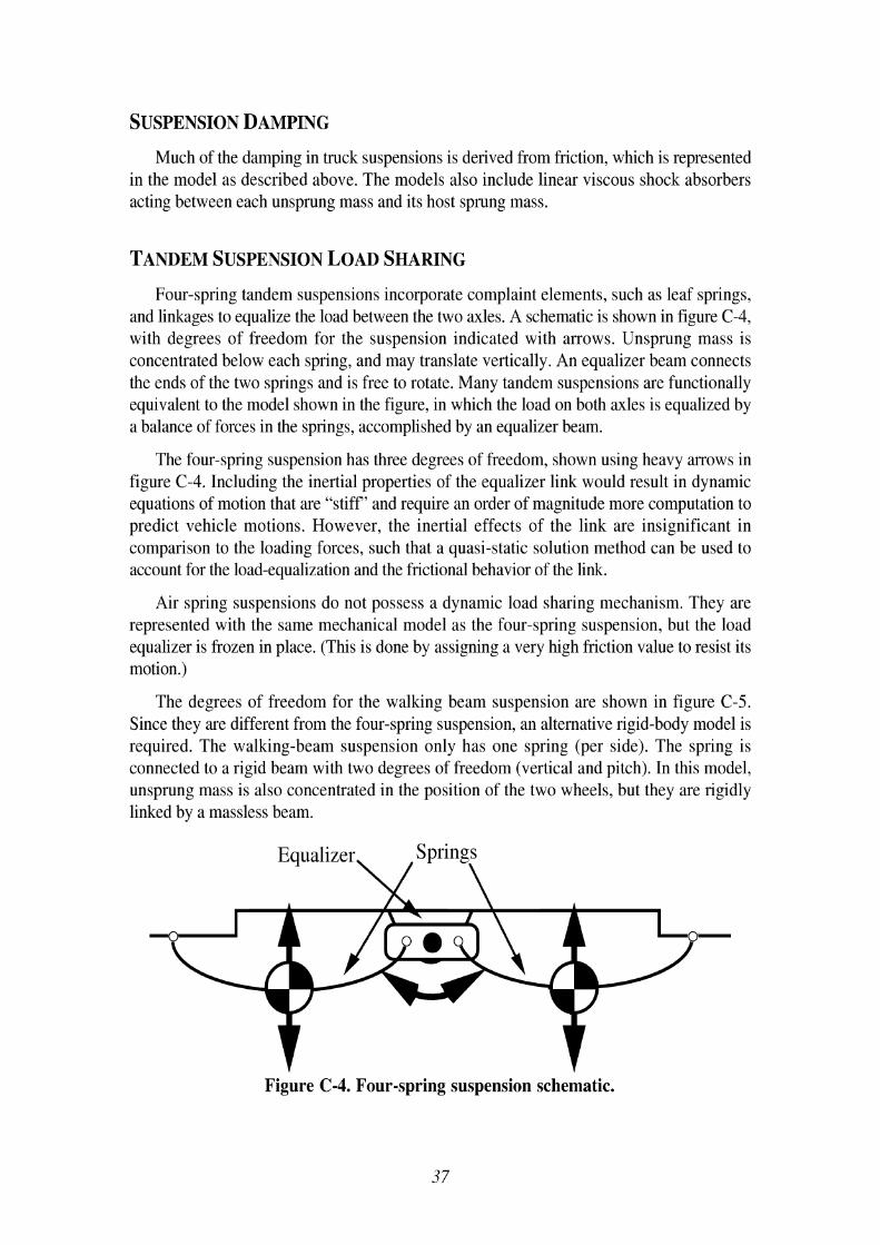
SUSPENSION DAMPING

Much of the damping in truck suspensions is derived from friction, which is represented in the model as described above. The models also include linear viscous shock absorbers acting between each unsprung mass and its host sprung mass.

TANDEM SUSPENSION LOAD SHARING

Four-spring tandem suspensions incorporate complaint elements, such as leaf springs, and linkages to equalize the load between the two axles. A schematic is shown in figure C-4, with degrees of freedom for the suspension indicated with arrows. Unsprung mass is concentrated below each spring, and may translate vertically. An equalizer beam connects the ends of the two springs and is free to rotate. Many tandem suspensions are functionally equivalent to the model shown in the figure, in which the load on both axles is equalized by a balance of forces in the springs, accomplished by an equalizer beam.

The four-spring suspension has three degrees of freedom, shown using heavy arrows in figure C-4. Including the inertial properties of the equalizer link would result in dynamic equations of motion that are "stiff' and require an order of magnitude more computation to predict vehicle motions. However, the inertial effects of the link are insignificant in comparison to the loading forces, such that a quasi-static solution method can be used to account for the load-equalization and the frictional behavior of the link.

Air spring suspensions do not possess a dynamic load sharing mechanism. They are represented with the same mechanical model as the four-spring suspension, but the load equalizer is frozen in place. (This is done by assigning a very high friction value to resist its motion.)

The degrees of freedom for the walking beam suspension are shown in figure C-5. Since they are different from the four-spring suspension, an alternative rigid-body model is required. The walking-beam suspension only has one spring (per side). The spring is connected to a rigid beam with two degrees of freedom (vertical and pitch). In this model, unsprung mass is also concentrated in the position of the two wheels, but they are rigidly linked by a massless beam.

Figure C-4. Four-spring suspension schematic.

37

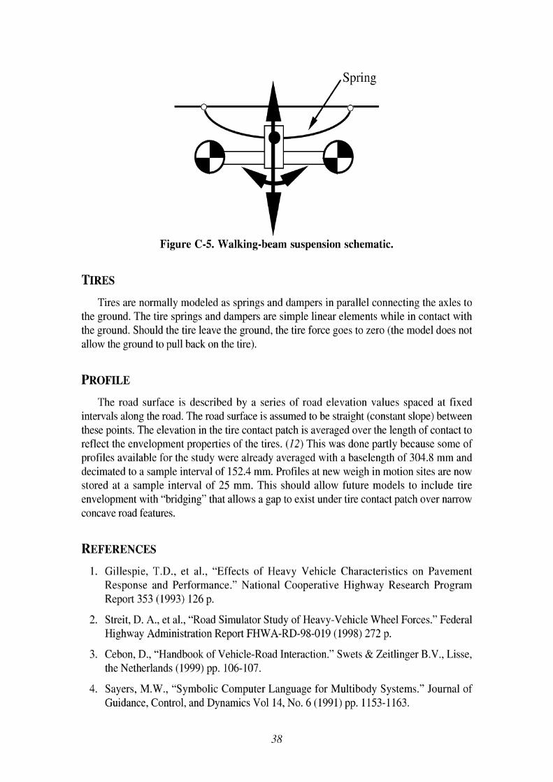
Figure C-5. Walking-beam suspension schematic.

TIRES

Tires are normally modeled as springs and dampers in parallel connecting the axles to the ground. The tire springs and dampers are simple linear elements while in contact with the ground. Should the tire leave the ground, the tire force goes to zero (the model does not allow the ground to pull back on the tire).

PROFILE

The road surface is described by a series of road elevation values spaced at fixed intervals along the road. The road surface is assumed to be straight (constant slope) between these points. The elevation in the tire contact patch is averaged over the length of contact to reflect the envelopment properties of the tires. (12) This was done partly because some of profiles available for the study were already averaged with a baselength of 304.8 mm and decimated to a sample interval of 152.4 mm. Profiles at new weigh in motion sites are now stored at a sample interval of 25 mm. This should allow future models to include tire envelopment with "bridging" that allows a gap to exist under tire contact patch over narrow concave road features.

REFERENCES

1. Gillespie, T.D., et al., "Effects of Heavy Vehicle Characteristics on Pavement Response and Performance." National Cooperative Highway Research Program Report 353 (1993) 126 p.

2. Streit, D. A,, et al., "Road Simulator Study of Heavy-Vehicle Wheel Forces." Federal Highway Administration Report FHWA-RD-98-019 (1998) 272 p.

3. Cebon, D., "Handbook of Vehicle-Road Interaction." Swets & Zeitlinger B.V., Lisse, the Netherlands (1999) pp. 106- 107.

4. Sayers, M.W., "Symbolic Computer Language for Multibody Systems." Journal of Guidance, Control, and Dynamics Vol 14, No. 6 (1991) pp. 1153-1 163.

5. Sayers, M.W., "Symbolic VectorJDyadic Multibody Formalism for Tree-Topology Systems." Journal of Guidance, Control, and Dynamics Vol 14, No. 6 (1991) pp. 1240- 1250.

6. Gillespie, T. D., and Karamihas, S. M., "The Feasibility of Multi-Sensor Weighing for Increased Accuracy of WIM." International Journal of Vehicle Design: Heavy Vehicle Systems, Vol. 3, Nos. 1-4 (1996) pp. 149-164.

7. Fancher, P.F., et al., "Measurement and Representation of the Mechanical Properties of Truck Leaf springs." Society of Automotive Engineers Paper 800905 (1980) 16 p.

8. Sayers, M. W. and Gillespie, T. D., "Dynamic Pavement Wheel Loading for Trucks with Tandem Suspensions." Proceedings, Symposium on the Dynamics of Vehicles on Roads and Tracks, Lisse, Swets and Zeitlinger (1984) pp. 517-533.

9. Gillespie, T. D., and Karamihas, S. M., "Characterizing the Road Damaging Dynamics of Truck Tandem Suspensions." Society of Automotive Engineers Paper No. 932994 (1993) 8 p.

10. Cole, D. J., and Cebon, D., "Validation of an Articulated Vehicle Simulation." Vehicle System Dynamics, Vol. 21, No. 4 (1992) pp. 197-224.

11. Winkler, C. B. and Hagan, M., "A Test Facility for Measurement of Heavy Vehicle Suspension Parameters." Transactions of the Society of Automotive Engineers, Vol. 89, Paper No. 800906 (1980) 29 p.

12. Gillespie, T.D., et al., "Calibration of Response-Type Road Roughness Measuring Systems." National Cooperative Highway Research Program Report 228 (1980) 81 p.

Appendix D: Truck Simulation Fleet

This appendix describes the mix of three-axle straight truck properties covered in the "simulation fleet" for verification of roughness criteria at weigh-in-motion (WIM) scale approaches. Overall, 109 combinations of suspension, tire, loading scheme, and body style appear in this fleet. These combinations do not represent a simple factorial matrix of possible parameter values. Rather, they are a set of typical three-axle straight trucks loaded in typical ways. Some combinations are somewhat unusual, so they were excluded. In addition, certain options are much more common than others, so they were combined with a greater number of loading schemes.

Certain parameters have a major influence on the results. These were drive axle suspension force-deflection characteristics, suspension damping, gross vehicle weight, and speed. (1) Care was taken to cover a reasonable range of these properties and include some diversity in them. Other parameters influenced the statistical performance of a simulated weigh scale very little. This was true of parameter values that simply do not vary much in practice, and of parameters that vary somewhat but do not have much impact on truck wheel loads. In these cases, variations in the parameter values were not allowed to increase the number of trucks in the virtual fleet. Often, a single standard value was chosen for the parameter.

Overall, the fleet included four body types, five steer axle suspensions, seven drive axle suspensions, and six loading schemes. Each vehicle was given an appropriate set of standard truck tires, and a small subset of the vehicles was fitted with wide-based single tires.

BODY TYPE

Four body types were included in the population of three axle straight trucks: (1) box, (2 ) flatbed and stake, (3) dump, and (4) refuse. Body type is not an explicit input to the simulation models. However, each body type is associated with a typical range of wheelbase and typical suspension mixes, as well as the likelihood of overload. Further, the body type helps determine the pitch moment of inertia of the empty vehicle and the mass distribution of the load.

Typical sets of steering axle and drive axle suspension were mounted to each body type. Overall, eleven mixes of suspension were assembled from five steering axle suspensions and seven drive axle suspensions in typical combinations. Table D-1 lists the suspensions and the associated unsprung weight for each.

All of the suspensions assigned to these vehicles were represented by parameters measured on real vehicles in the UMTRI Suspension Parameter Measurement Facility. (2) They were chosen from a database of over 160 heavy truck suspensions that were tested at UMTRI since 1984. Few of these data are published. (3-5) The suspensions listed in table

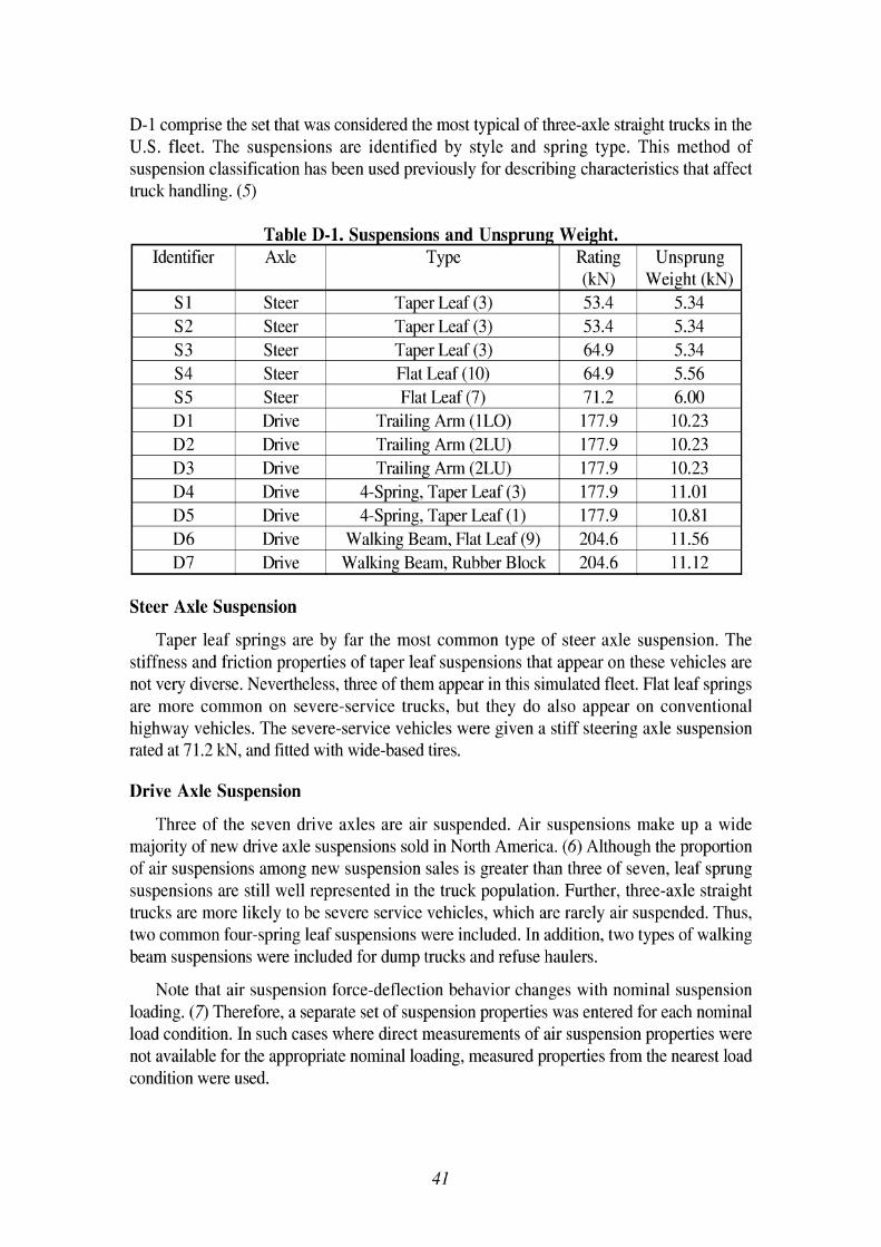
D-1 comprise the set that was considered the most typical of three-axle straight trucks in the U.S. fleet. The suspensions are identified by style and spring type. This method of suspension classification has been used previously for describing characteristics that affect truck handling. (5)

Steer Axle Suspension

Table D-1. Suspensions and Unsprung Weight.

Taper leaf springs are by far the most common type of steer axle suspension. The stiffness and friction properties of taper leaf suspensions that appear on these vehicles are not very diverse. Nevertheless, three of them appear in this simulated fleet. Flat leaf springs are more common on severe-service trucks, but they do also appear on conventional highway vehicles. The severe-service vehicles were given a stiff steering axle suspension rated at 7 1.2 kN, and fitted with wide-based tires.

Identifier

Drive Axle Suspension

Three of the seven drive axles are air suspended. Air suspensions make up a wide majority of new drive axle suspensions sold in North America. (6) Although the proportion of air suspensions among new suspension sales is greater than three of seven, leaf sprung suspensions are still well represented in the truck population. Further, three-axle straight trucks are more likely to be severe service vehicles, which are rarely air suspended. Thus, two common four-spring leaf suspensions were included. In addition, two types of walking beam suspensions were included for dump trucks and refuse haulers.

Axle

Note that air suspension force-deflection behavior changes with nominal suspension loading. (7) Therefore, a separate set of suspension properties was entered for each nominal load condition. In such cases where direct measurements of air suspension properties were not available for the appropriate nominal loading, measured properties from the nearest load condition were used.

TY pe Rating (kN)

Unsprung Weight (kN)

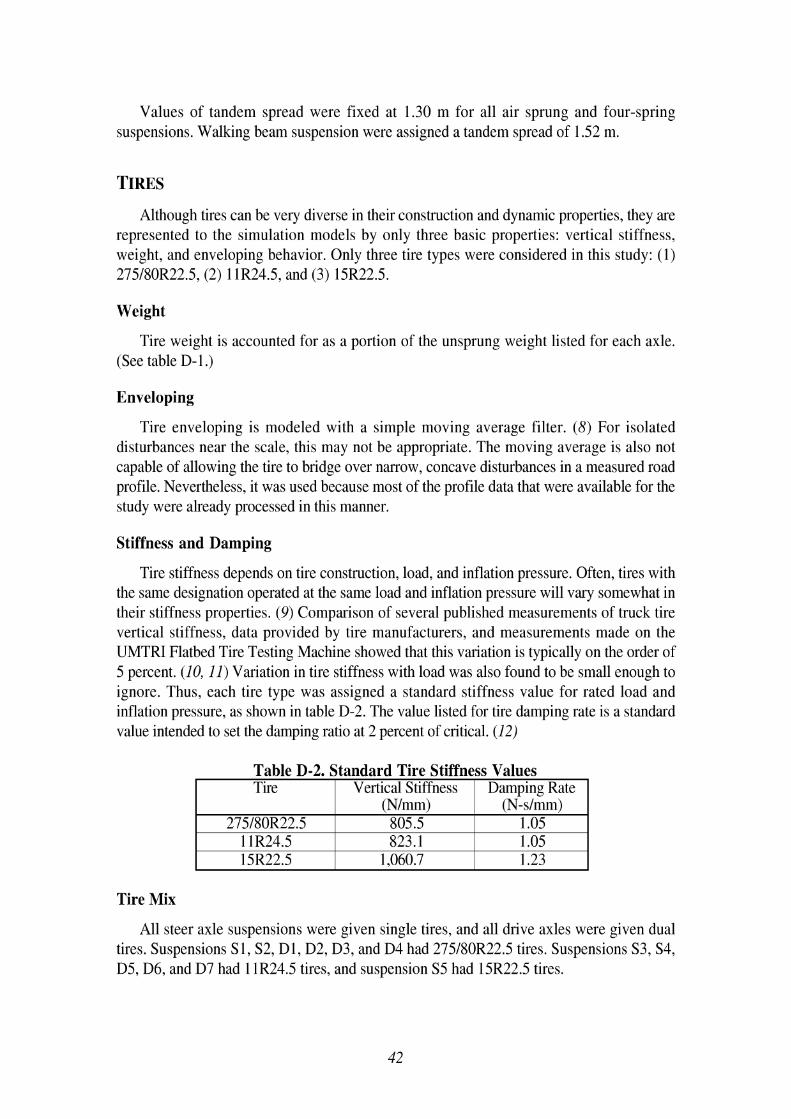
Values of tandem spread were fixed at 1.30 m for all air sprung and four-spring suspensions. Walking beam suspension were assigned a tandem spread of 1.52 m.

TIRES

Although tires can be very diverse in their construction and dynamic properties, they are represented to the simulation models by only three basic properties: vertical stiffness, weight, and enveloping behavior. Only three tire types were considered in this study: (1) 2751801322.5, (2) 11R24.5, and (3) 151322.5.

Weight

Tire weight is accounted for as a portion of the unsprung weight listed for each axle. (See table D- 1 .)

Enveloping

Tire enveloping is modeled with a simple moving average filter. (8) For isolated disturbances near the scale, this may not be appropriate. The moving average is also not capable of allowing the tire to bridge over narrow, concave disturbances in a measured road profile. Nevertheless, it was used because most of the profile data that were available for the study were already processed in this manner.

Stiffness and Damping

Tire stiffness depends on tire construction, load, and inflation pressure. Often, tires with the same designation operated at the same load and inflation pressure will vary somewhat in their stiffness properties. (9) Comparison of several published measurements of truck tire vertical stiffness, data provided by tire manufacturers, and measurements made on the UMTRI Flatbed Tire Testing Machine showed that this variation is typically on the order of 5 percent. (10, 11) Variation in tire stiffness with load was also found to be small enough to ignore. Thus, each tire type was assigned a standard stiffness value for rated load and inflation pressure, as shown in table D-2. The value listed for tire damping rate is a standard value intended to set the damping ratio at 2 percent of critical. (12)

Table D-2. Standard Tire Stiffness Values

(Nlmm) (N-slmm) 2751801322.5 805.5

1 lR24.5 823.1 15R22.5 1,060.7

Tire Mix

All steer axle suspensions were given single tires, and all drive axles were given dual tires. Suspensions S1, S2, D l , D2, D3, and D4 had 275180R22.5 tires. Suspensions S3, S4, D5, D6, and D7 had 111324.5 tires, and suspension S5 had 15R22.5 tires.

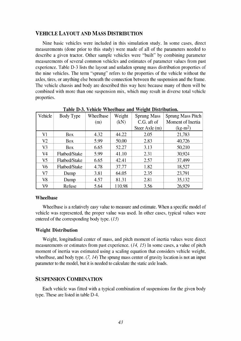
VEHICLE LAYOUT AND MASS DISTRIBUTION

Nine basic vehicles were included in this simulation study. In some cases, direct measurements (done prior to this study) were made of all of the parameters needed to describe a given tractor. Other sample vehicles were "built" by combining parameter measurements of several common vehicles and estimates of parameter values from past experience. Table D-3 lists the layout and unladen sprung mass distribution properties of the nine vehicles. The term "sprung" refers to the properties of the vehicle without the axles, tires, or anything else beneath the connection between the suspension and the frame. The vehicle chassis and body are described this way here because many of them will be combined with more than one suspension mix, which may result in diverse total vehicle properties.

Wheelbase

Table D-3. Vehicle Wheelbase and Weight Distribution.

Wheelbase is a relatively easy value to measure and estimate. When a specific model of vehicle was represented, the proper value was used. In other cases, typical values were entered of the corresponding body type. (1 3)

Vehicle

V1 V2 V3 V4 V5 V6 V7 V8 V9

Weight Distribution

Weight, longitudinal center of mass, and pitch moment of inertia values were direct measurements or estimates from past experience. (14, 15) In some cases, a value of pitch moment of inertia was estimated using a scaling equation that considers vehicle weight, wheelbase, and body type. (7, 14) The sprung mass center of gravity location is not an input parameter to the model, but it is needed to calculate the static axle loads.

Body Type

Box Box Box

FlatbedIStake FlatbedIStake FlatbedIStake

Dump Dump Refuse

SUSPENSION COMBINATION

Each vehicle was fitted with a typical combination of suspensions for the given body type. These are listed in table D-4.

Wheelbase (m)

4.32 5.99 6.65 5.99 6.65 4.78 3.81 4.57 5.64

Weight (kN)

44.22 50.00 52.27 41.10 42.4 1 37.77 64.05 81.31 110.98

Sprung Mass C.G. aft of

Steer Axle (m) 2.05 2.83 3.13 2.3 1 2.57 1.82 2.35 2.81 3.56

Sprung Mass Pitch Moment of Inertia

(kg-m2) 21,783 40,726 50,210 30,924 37,499 18,527 23,791 35,132 26,929

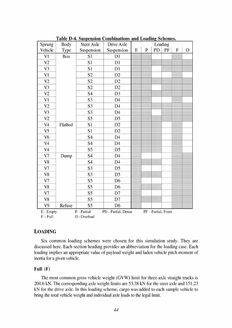
E - Empty F - Full

P - Partial PD - Partial, Dense PF - Partial, Front 0 - Overload

LOADING

Six common loading schemes were chosen for this simulation study. They are discussed here. Each section heading provides an abbreviation for the loading case. Each loading implies an appropriate value of payload weight and laden vehicle pitch moment of inertia for a given vehicle.

Full (F)

The most common gross vehicle weight (GVW) limit for three-axle straight trucks is 204.6 kN. The corresponding axle weight limits are 53.38 kN for the steer axle and 151.23 kN for the drive axle. In this loading scheme, cargo was added to each sample vehicle to bring the total vehicle weight and individual axle loads to the legal limit.

All vehicles were simulated in the full condition. In the case of box trucks, the load was assumed to extend most of the length of the box, and was about 1.8 m high. For dump trucks, flatbed and stake trucks, and refuse haulers, the load was assumed to be about 1.2 m high.

Overloaded ( 0 )

Overloaded box trucks were given 4.45 kN of extra payload, with the same mass distribution as the payload for the full condition. Overloaded dump trucks were given 3.56 kN of extra payload, with the same mass distribution as the payload for the full condition. The overloaded refuse hauler was given 6.22 kN of extra payload, which was added to the top of the full condition by extending the load height to about 1.8 m. Flatbed trucks were not simulated with overload.

Empty vehicles make up a significant portion of the trucks measured at WIM scales. (16, 17) In this loading scheme, each vehicle was simply combined with no payload. Each vehicle was simulated in the empty condition.

Partial (P)

Partial loading was simulated by cutting the load used for the full case in half, but retaining the load distribution. This is meant to simulate load that is not dense enough to full load a vehicle. This loading scheme was avoided on some dump trucks and refuse haulers, because they commonly carry dense load.

Partial, Forward (PF)

Another version of partial loading was simulated in which the load was concentrated at the from half of the cargo area. Only box trucks were simulated this way, and only some those with a long wheelbase.

Partial, Dense

Yet another version of partial loading was included in which the load was assumed to be very dense, so it was distributed along the length of the vehicle, but the load was given a low overall height. This loading was applied to all of the flatbed tmcks, and some of the others.

SUSPENSION DAMPING

Suspension shock absorber damping was found in preliminary vehicle simulations to have a significant impact on the dynamic loading experienced at the weight scales. Unfortunately, little data on measured truck shock absorber force-velocity appear in the literature. The shock absorber damping coefficient values that were used represent the experience of the engineers at UMTRI. The relative contribution of the shock absorbers to overall suspension damping depends on the level of friction present in the suspension force- deflection characteristic. In general, the drive and trailer axle suspension exhibited damping

ratio values of 15-20 percent under the crude characterization provided by simulating truck vibration after passing over a large step.

Since shock absorber damping was found to be so important to the results, all vehicles were simulated with two damping cases. The first case, with new shock absorbers, is covered by the 15-20 percent overall damping ratio. The second case is worn shock absorbers. This case is approximated by reducing the trailer axle damping coefficient values to 25 percent of their original values and the tractor shock absorber damping coefficient values to 50 percent of the original values. The tractor is not allowed to lose as much of its damping power as the trailer, because the driver is expected to complain if the damping gets too low.

All vehicles were simulated at three speeds: 72.4,88.5, and 104.6 kph.

Of the 109 vehicles in the "fleet". 25 were full, 25 were empty, 17 were overloaded, and 42 were partially loaded. Of the 42 partially loaded vehicles, 8 had loading that was biased toward the front, 14 had dense loads, and 20 had loading that filled the cargo compartment. The 109 vehicles included 54 box trucks, 20 flatbed and stake trucks, 32 dump trucks, and 3 refuse haulers. These vehicles also included 58 taper leaf steer axle suspensions and 41 flat leaf steer axle suspensions. The drive axles included 42 air suspensions, 48 four-spring suspensions, and 19 walking-beam suspensions.

When the vehicle, damping, and speed options were all combined, the total number of simulation runs per profile was 654.

REFERENCES

1. Karamihas, S. M. and Gillespie, T. D., "Smoothness Criteria for WIM Scale Approaches." University of Michigan Transportation Research Institute Report UMTRI-2002-37 (2002) 81 p.

2. Winkler, C. B. and Hagan, M., "A Test Facility for Measurement of Heavy Vehicle Suspension Parameters." Transactions of the Society of Automotive Engineers, Vol. 89, Paper No. 800906 (1980) 29 p.

3. Winkler, C. B, et, al., "Parameter Measurements of a Highway Tractor Semitrailer." National Highway Traffic Safety Administration Vehicle Research and Test Center Report (1995) 159 p.

4. Ervin, R., et, al., "Two Active Systems for Enhancing Dynamic Stability in Heavy Truck Operations." University of Michigan Transportation Research Institute Report UMTRI-98-39 (1998) 216 p.

5. Winkler, C. B., et. al., "Roll Stability Performance of Heavy Vehicle Suspensions.'' Transactions of the Society of Automotive Engineers, Vol. 101, Paper No. 922426 (1992) 9 p.

6. Hajek, J. J. and Selezneva, 0. I., "Estimating Cumulative Traffic Loads, Final Report for Phase I." Federal Highway Administration Publication No. FHWA-RD-00-054 (2000) 202 p.

7. Segel, L., et. al., "Mechanics of Heavy-Duty Trucks and Truck Combinations." Engineering Summer Conferences, University of Michigan College of Engineering (2002).

8. Gillespie, T. D., et. al., "Effect of Heavy Vehicle Characteristics on Pavement Response and Performance." National Cooperative Highway Research Program Report 353 (1993) 126 p.

9. Pottinger, M. G., et. al. "Force and Moment Properties of a Small Sample of Tire Specifications: Drive, Steer, and Trailer with Evolution from New to Naturally Worn- out to Retreaded considered." Society of Automotive Report No. SAE 982748. (1998) 13 P.

10. Pezo, R. F., et. al., "Truck Tire Pavement Contact Pressure Distribution Characteristics for the Bias Goodyear 18-22.5, the Radial Michelin 275180W24.5, the Radial Michelin 255170W22.5, and the Radial Goodyear 11R24.5 Tires" Center for Transportation Research at the University of Texas at Austin, Research Report 1190- 2F (1989) 56 p.

11. Streit, D. A., et. al. "Road Simulator Study of Heavy-Vehicle Wheel Forces." Federal Highway Administration Report FHWA-RD-98-019 (1998) 272 p.

12. Karamihas, S. M. and Gillespie, T. D., "Characterizing Trucks for Dynamic Load Prediction." International Journal of Vehicle Design, Heavy Vehicle Systems, Vol. 1, No. 1 (1993) pp. 3-19.

13. "2001 Diesel Truck Index." Truck Index, Inc., Santa Ana, CA (2001) 300 p.

14. Fancher, P. S., et, al., "A Factbook of the Mechanical Properties of the Components for Single Unit and Articulated Heavy Trucks." National Highway Traffic Safety Administration Report DOT HS 807 125 (1986) 190 p.

15. Winkler, C. B., "Inertial Properties of Commercial Vehicles." University of Michigan Transportation Research Institute Report UMTRI-83-17, Volume 2 (1983) 25 p.

16. Ott, W. C. and Papagiannakis, A. T., "Weigh-in-Motion Data Quality Assurance Based on 3-S2 Steer Axle Load Analysis." Transportation Research Record 1536 (1996) pp. 12-18.

17. Schmoyer, R., et. al., "Analysis of Vehicle Classification and Truck Weight Data of the New England States." Oak Ridge National Laboratories Report (1998) 125 p.