A seismic hazard scenario in the Sikkim Himalaya from seismotectonics, spectral amplification, source parameterization, and spectral attenuation laws using strong motion seismometry

A seismic hazard scenario in the Sikkim Himalaya from

seismotectonics, spectral amplification, source

parameterization, and spectral attenuation

laws using strong motion seismometry

Sankar Kumar Nath, Madhav Vyas, Indrajit Pal, and Probal SenguptaDepartment of Geology and Geophysics, Indian Institute of Technology, Kharagpur, India

Received 1 June 2004; revised 6 October 2004; accepted 13 October 2004; published 6 January 2005.

[1] In this paper, we present a seismic hazard map of the Indian Himalayan State ofSikkim, lying between Nepal and Bhutan Himalaya, in terms of horizontal peak groundaccelerations with 10% exceedance probability over the next 50 years. These figures,the first for the region, were calculated through a stepwise process based on (1) anestimation of the maximum credible earthquake (MCE) from the seismicity of the regionand Global Seismic Hazard Assessment Program considerations and (2) fourseismotectonic parameters abstracted from accelerograms recorded at nine stations of theSikkim Strong Motion Array, specifically installed for this study. The latter include (1) thefrequency-dependent power law for the shear wave quality factor, QS, (2) the site responsefunction at each station using receiver function analysis and generalized inversion,(3) source parameterization of various events recorded by the array and application of theresulting relationships between M0 and MW, and corner frequency, fc and MW to simulatespectral accelerations due to higher-magnitude events corresponding to the estimatedMCE, and (4) abstraction of regional as well as site specific local spectral attenuation laws atdifferent geometrically central frequencies in low-, moderate-, and high-frequency bands.

Citation: Nath, S. K., M. Vyas, I. Pal, and P. Sengupta (2005), A seismic hazard scenario in the Sikkim Himalaya from

seismotectonics, spectral amplification, source parameterization, and spectral attenuation laws using strong motion seismometry,

J. Geophys. Res., 110, B01301, doi:10.1029/2004JB003199.

1. Introduction

[2] The Sikkim Himalaya shares high seismicity of thenortheast India and is currently bracing up to develop itsnatural resources toward improving the quality of life of thepeople, in a high earthquake prone environment. An im-portant scientific component of these endeavors is thereforethe creation of hazard mitigation knowledge products,notably, seismic hazard maps, which is the subject ofresearch reported in this paper.[3] The State of Sikkim lies at the eastern edge of the

rupture zone of the 1934 M = 8.4 Bihar Nepal earthquakewhich claimed about 11,000 lives and caused an intensity ofVIII in the Sikkim Himalaya [Geological Survey of India(GSI), 1939]. It was severely shaken again by the 1988Ms =6.6 earthquake which ruptured a deeper part of the samezone, the isoseismal VII passing through its capital town ofGangtok in an approximately NE-SW direction. Severalhouses in the town were badly damaged, while power andother communication system installations suffered subsi-dence and there occurred a series of disrupting landslides.Earthquake activity attests to the progress of a continuingepoch of high seismicity in the region, characterized by analmost continuous burst of seismic energy.

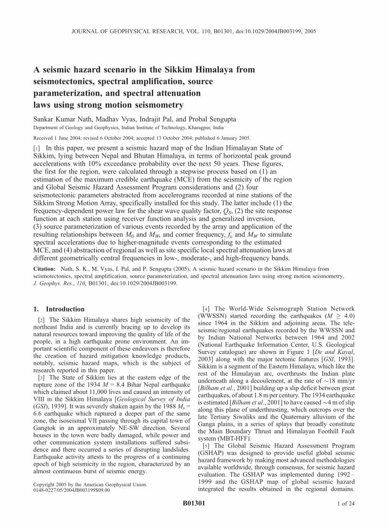
[4] The World-Wide Seismograph Station Network(WWSSN) started recording the earthquakes (M � 4.0)since 1964 in the Sikkim and adjoining areas. The tele-seismic/regional earthquakes recorded by the WWSSN andby Indian National Networks between 1964 and 2002(National Earthquake Information Center, U.S. GeologicalSurvey catalogue) are shown in Figure 1 [De and Kayal,2003] along with the major tectonic features [GSI, 1993].Sikkim is a segment of the Eastern Himalaya, which like therest of the Himalayan arc, overthrusts the Indian plateunderneath along a decoulement, at the rate of �18 mm/yr[Bilham et al., 2001] building up a slip deficit between greatearthquakes, of about 1.8m per century. The 1934 earthquakeis estimated [Bilham et al., 2001] to have caused�4 m of slipalong this plane of underthrusting, which outcrops over thelate Tertiary Siwaliks and the Quaternary alluvium of theGanga plains, in a series of splays that broadly constitutethe Main Boundary Thrust and Himalayan Foothill Faultsystem (MBT-HFF).[5] The Global Seismic Hazard Assessment Program

(GSHAP) was designed to provide useful global seismichazard framework by making most advanced methodologiesavailable worldwide, through consensus, for seismic hazardevaluation. The GSHAP was implemented during 1992–1999 and the GSHAP map of global seismic hazardintegrated the results obtained in the regional domains.

JOURNAL OF GEOPHYSICAL RESEARCH, VOL. 110, B01301, doi:10.1029/2004JB003199, 2005

Copyright 2005 by the American Geophysical Union.0148-0227/05/2004JB003199$09.00

B01301 1 of 24

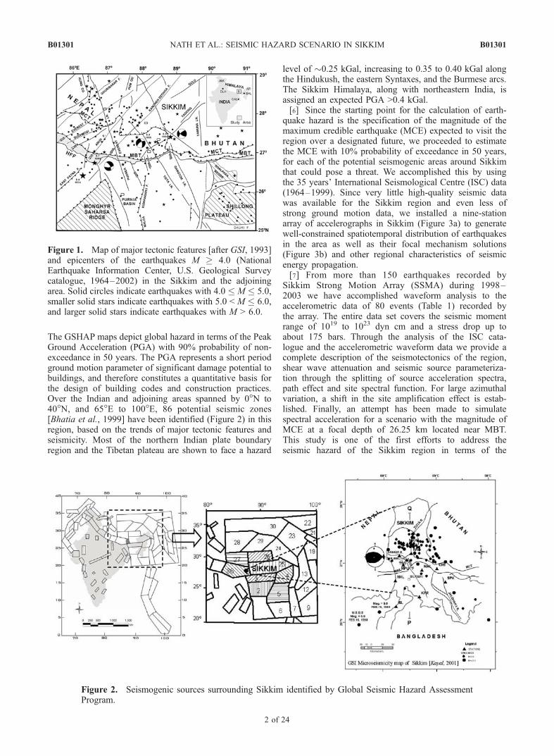
The GSHAP maps depict global hazard in terms of the PeakGround Acceleration (PGA) with 90% probability of non-exceedance in 50 years. The PGA represents a short periodground motion parameter of significant damage potential tobuildings, and therefore constitutes a quantitative basis forthe design of building codes and construction practices.Over the Indian and adjoining areas spanned by 0�N to40�N, and 65�E to 100�E, 86 potential seismic zones[Bhatia et al., 1999] have been identified (Figure 2) in thisregion, based on the trends of major tectonic features andseismicity. Most of the northern Indian plate boundaryregion and the Tibetan plateau are shown to face a hazard

level of �0.25 kGal, increasing to 0.35 to 0.40 kGal alongthe Hindukush, the eastern Syntaxes, and the Burmese arcs.The Sikkim Himalaya, along with northeastern India, isassigned an expected PGA >0.4 kGal.[6] Since the starting point for the calculation of earth-

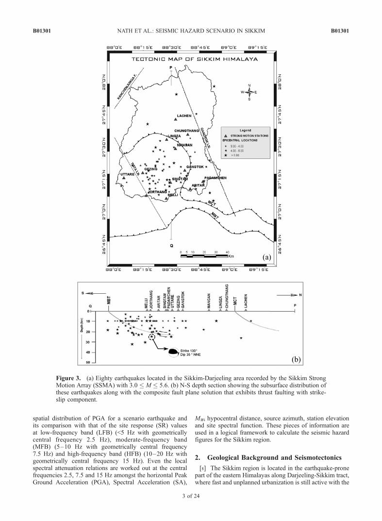
quake hazard is the specification of the magnitude of themaximum credible earthquake (MCE) expected to visit theregion over a designated future, we proceeded to estimatethe MCE with 10% probability of exceedance in 50 years,for each of the potential seismogenic areas around Sikkimthat could pose a threat. We accomplished this by usingthe 35 years’ International Seismological Centre (ISC) data(1964–1999). Since very little high-quality seismic datawas available for the Sikkim region and even less ofstrong ground motion data, we installed a nine-stationarray of accelerographs in Sikkim (Figure 3a) to generatewell-constrained spatiotemporal distribution of earthquakesin the area as well as their focal mechanism solutions(Figure 3b) and other regional characteristics of seismicenergy propagation.[7] From more than 150 earthquakes recorded by

Sikkim Strong Motion Array (SSMA) during 1998–2003 we have accomplished waveform analysis to theaccelerometric data of 80 events (Table 1) recorded bythe array. The entire data set covers the seismic momentrange of 1019 to 1023 dyn cm and a stress drop up toabout 175 bars. Through the analysis of the ISC cata-logue and the accelerometric waveform data we provide acomplete description of the seismotectonics of the region,shear wave attenuation and seismic source parameteriza-tion through the splitting of source acceleration spectra,path effect and site spectral function. For large azimuthalvariation, a shift in the site amplification effect is estab-lished. Finally, an attempt has been made to simulatespectral acceleration for a scenario with the magnitude ofMCE at a focal depth of 26.25 km located near MBT.This study is one of the first efforts to address theseismic hazard of the Sikkim region in terms of the

Figure 2. Seismogenic sources surrounding Sikkim identified by Global Seismic Hazard AssessmentProgram.

Figure 1. Map of major tectonic features [after GSI, 1993]and epicenters of the earthquakes M � 4.0 (NationalEarthquake Information Center, U.S. Geological Surveycatalogue, 1964–2002) in the Sikkim and the adjoiningarea. Solid circles indicate earthquakes with 4.0 � M � 5.0,smaller solid stars indicate earthquakes with 5.0 < M � 6.0,and larger solid stars indicate earthquakes with M > 6.0.

B01301 NATH ET AL.: SEISMIC HAZARD SCENARIO IN SIKKIM

2 of 24

B01301

spatial distribution of PGA for a scenario earthquake andits comparison with that of the site response (SR) valuesat low-frequency band (LFB) (<5 Hz with geometricallycentral frequency 2.5 Hz), moderate-frequency band(MFB) (5–10 Hz with geometrically central frequency7.5 Hz) and high-frequency band (HFB) (10–20 Hz withgeometrically central frequency 15 Hz). Even the localspectral attenuation relations are worked out at the centralfrequencies 2.5, 7.5 and 15 Hz amongst the horizontal PeakGround Acceleration (PGA), Spectral Acceleration (SA),

MW, hypocentral distance, source azimuth, station elevationand site spectral function. These pieces of information areused in a logical framework to calculate the seismic hazardfigures for the Sikkim region.

2. Geological Background and Seismotectonics

[8] The Sikkim region is located in the earthquake-pronepart of the eastern Himalayas along Darjeeling-Sikkim tract,where fast and unplanned urbanization is still active with the

Figure 3. (a) Eighty earthquakes located in the Sikkim-Darjeeling area recorded by the Sikkim StrongMotion Array (SSMA) with 3.0 � M � 5.6. (b) N-S depth section showing the subsurface distribution ofthese earthquakes along with the composite fault plane solution that exhibits thrust faulting with strike-slip component.


3 of 24

B01301

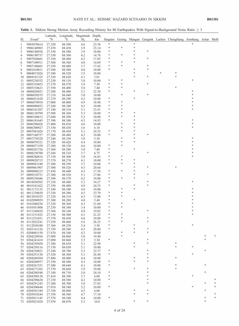
Table 1. Sikkim Strong Motion Array Recording History for 80 Earthquakes With Signal-to-Background Noise Ratio � 3

Sl. EventaLatitude,

�NLongitude,

�EMagnitude

ML

Depth,km Singtam Gezing Mangan Gangtok Lachen Chungthang Jorethang Aritar Melli

1 9903070614 27.250 88.390 4.6 23.58 * * *2 9906140903 27.470 88.430 3.9 23.14 * * *3 9906180936 27.350 88.580 3.9 10.00 * * *4 9906190757 27.350 88.360 4.2 14.76 * * *5 9907020601 27.250 88.480 4.2 17.85 * * *6 9907100911 27.360 88.360 4.0 14.69 * * *7 9907140601 27.250 88.480 3.7 17.43 * * *8 0001010011 27.300 88.580 4.0 10.00 * * *9 0004071026 27.380 88.520 3.5 10.00 * * *10 0004181325 27.520 88.630 4.1 3.01 * * *11 0005230352 27.230 88.110 3.0 10.00 * * *12 0005310453 27.270 88.570 3.8 7.50 * * *13 0005310621 27.550 88.400 5.0 7.40 * * *14 0006020851 27.200 88.480 5.1 22.30 * * *15 0006030555 27.210 88.440 3.0 10.00 * * *16 0006031628 27.270 88.290 4.2 10.00 * * *17 0006070910 27.000 88.000 4.9 18.98 * * *18 0006080832 27.240 88.340 4.2 10.00 * * *19 0006101207 27.180 88.310 5.1 23.41 * * *20 0006130709 27.500 88.360 5.3 10.00 * * *21 0006160612 27.680 88.290 5.2 10.00 * * *22 0006181645 27.390 88.380 4.3 14.92 * * *23 0006290426 27.400 88.830 4.6 10.00 * * *24 0006300927 27.330 88.430 3.6 6.10 * * *25 0007041026 27.170 88.450 5.1 24.52 * * *26 0007160757 27.200 88.480 4.2 10.00 * * *27 0007270320 27.240 88.250 3.8 5.30 * * *28 0008070321 27.320 88.420 4.4 10.00 * * *29 0008071359 27.280 88.330 4.6 10.00 * * *30 0008201726 27.360 88.280 3.0 7.80 * * *31 0008230700 27.260 88.310 3.7 6.75 * * *32 0008280816 27.150 88.300 3.9 16.83 * * *33 0009020715 27.370 88.270 4.1 10.00 * * *34 0009041248 27.280 88.350 3.7 10.00 * * *35 0009061907 27.500 88.520 4.5 20.64 * * *36 0009080215 27.430 88.440 4.3 17.58 * * *37 0009210751 27.380 88.520 5.1 17.86 * * *38 0009250446 27.390 88.370 4.2 10.00 * * *39 0010030502 27.230 88.480 5.3 34.27 * * *40 0010181422 27.350 88.480 4.9 24.53 * * *41 0011172135 27.240 88.540 4.8 10.00 * * *42 0011230650 27.250 88.300 4.5 23.79 * * *43 0012010355 27.220 88.310 4.3 13.00 * * *44 0102090959 27.300 88.280 4.0 5.40 * * *45 0101040236 27.220 88.360 4.3 21.60 * * *46 0101051808 27.230 88.380 3.4 10.00 * * *47 0111160424 27.360 88.160 4.8 19.02 * * *48 0111151432 27.150 88.300 4.1 21.23 * * *49 0111231031 27.370 88.430 4.8 10.00 * * *50 0112022241 27.250 88.460 5.6 26.25 * * *51 0112030100 27.360 88.230 3.4 3.50 * * *52 0203161126 27.350 88.580 4.5 20.00 * * *53 0204081150 27.470 88.340 4.3 10.00 * * *54 0204220936 27.090 88.860 5.0 19.40 * * *55 0204241418 27.090 88.860 3.5 5.30 * * *56 0204250458 27.280 88.630 5.1 22.90 * * *57 0204250116 27.150 88.830 5.1 10.00 * * *58 0204250821 27.240 88.780 5.3 32.37 * * *59 0204251130 27.320 88.300 5.1 26.40 * * *60 0204260304 27.480 88.400 4.4 10.00 * * *61 0204260957 27.350 88.580 4.3 10.00 * * *62 0204261551 27.300 88.640 4.1 10.00 * * *63 0204271203 27.570 88.660 3.9 10.00 * * *64 0204280548 27.180 88.710 5.0 24.10 * * *65 0204290138 27.410 88.390 3.7 6.00 * * *66 0204290628 27.230 88.580 4.2 10.00 * * *67 0204291243 27.200 88.700 5.0 27.83 * * *68 0204300646 27.910 88.540 5.2 10.00 * * *69 0204301349 27.350 88.800 4.5 6.00 * * *70 0205010244 27.350 88.580 4.7 17.10 * * *71 0205011145 27.570 88.540 4.4 10.00 * * *72 0205021028 27.970 88.870 5.3 10.0 * * *


4 of 24

B01301

incidence of a good number of large earthquakes. Mostworkers have divided the Himalayas into a series of longi-tudinal tectonostratigraphic domains, such as, (1) Sub Hima-layas, (2) Lesser Himalayas, (3) Higher Himalayas, and(4) Tethys Himalayas (Figure 4a), which are separated bymajor dislocation zones. In the Sikkim region, the differentlithological units are disposed in an arcuate regional foldpattern. The ‘‘core’’ of the region is occupied by the LesserHimalayan low-grade metapelites, interbanded psammitebelonging to Daling Group (Proterozoic to Mesozoic). TheLingtse-granitoid gneiss occurs within the Daling Groupof rocks. The distal parts of the region are characterizedby medium- to high-grade crystalline rocks of the HigherHimalayan Belt (Higher Himalayan Crystalline Complex,HHC). A prominent ductile shear zone, the Main CentralThrust, separates the two belts. In this region, the MainCentral Thrust (MCT) is the southernmost one of a numberof northward dipping ductile shear zones within the HigherHimalayan Crystalline Complex. Gondwana (Carboniferous-Permian) and molasse-type Siwalik (Miocene-Pliocene)sedimentary rocks of the Sub-Himalayan Zone occur inthe southern part of the region. In the extreme north, a thickpile of Cambrian to Eocene fossiliferous sediments of theTethyan Zone (Tethyan sedimentary sequence, Figure 4a)overlies the HHC on the hanging wall side of a series ofnorth dipping normal faults constituting the South TibetanDetachment System (STDS) [Gansser, 1964]. The HHCconsists predominantly of high-grade pelitic migmatiteswith numerous layers of calc-silicate rocks and quartzites.Small bodies of metabasites and granites are also present inHHC. At places, several subsidiary thrusts are presentbetween MCT and MBT. Besides these thrusts, severalapproximately N-S trending gravity faults are also present.The structural configuration of this foredeep region isarchitectured by a set of near N-S faults, resulting in thedevelopment of alternate horst and graben structures. Alongwith the transverse faults, several lineaments cutting acrossthe Himalayan belt are also present. These exhibit north-easterly and northwesterly trends. The Kanchanjunga line-ament extends from the foredeep to inside the Himalayanbelt. Other prominent lineaments include NW-SE trendingTista and Gangtok lineaments [Narula et al., 2000]. Thoughthe MCT has been identified as a single tectonic plane inNepal Himalaya [Bordet, 1973] there are differences ofopinion about the definition of MCT in the eastern Hima-laya. Raina and Srivastava [1980] considered the MCT tobe tectonic plane between the Kanchenjunga gneiss andParo group of Bhutan on one side and the Darjeeling gneissand the Thimpu gneiss on the other (MCT-I) as proposedby Jangpangi [1979]. This tectonic plane extends eastward

in Arunachal Himalaya and demarcates the boundary be-tween the Lumla/Sela Group in the north and BomdilaGroup to the south. The other dislocation plane, consideredas MCT-II, separates the Darjeeling gneiss/Chungthan for-mation/Bomdila Group from the Daling and Shumar forma-tion [Acharyya and Ray, 1977; Sinha Roy, 1988]. Because ofthe nature of tectonic transport and topography, the outcroppattern of all these regional thrust surfaces has assumed asinuous shape in the map. All along the eastern Himalayamobile belt, there are many cross anticlinal/antiformal struc-tures, namely, Arun anticline in east Nepal, Rangit anticlinein Sikkim, Shumar antiform in Bhutan and Shyom antiforminArunachal Pradesh. All the Himalayan thrusts are traceablearound these anticlines [Nandy, 2001]. Deep erosion alongsome of the anticlines/antiforms has generated some well-known window structures in Himalayan fold-thrust belt.These are Rangit window in Sikkim, Kuru half window inBhutan and Siang window in Arunachal Pradesh. In Rangitwindow the para-autochthonous Gondwana and Buxa aresurrounded by allochthonous Daling rocks and Darjeelinggneiss over the MCT-II. The detailed petrographic provincesalong with the geomorphotectonic features are given inFigure 4b [Narula et al., 2000].[9] The focal mechanism solutions and other regional

characteristics of seismic energy propagation are alsoworked out for the earthquakes (Table 1) recorded bySSMA. The depth section as given in Figure 3b exhibitsmajor concentration of events surrounding MBT, the highestmagnitude being 5.6 for event 50 just below MBT at a focaldepth of 26.25 km. This earthquake is centrally located withrespect to the recording stations, thereby having a goodsource azimuthal coverage. The composite fault planesolution of this event along with others in the proximityof MBT suggests thrust faulting with strike-slip componentwith a dip of 35�NNE striking at 130�.

3. Data and Methodology

[10] A semipermanent nine-station strong motion array inSikkim established by Indian Institute of Technology (IIT),Kharagpur, India has been operative since 1998. One Kine-metrics Altus K2 and eight Kinemetrics Altus ETNA highdynamic range strong motion accelerographs have beeninstalled to continuously monitor the signals that satisfyevent detection criteria. A trigger level of 0.02% of the fullscale (2 kGal) and a sampling of 200 samples/s is set forthe data recording. The dynamic range of the systems is108 dB at 200 samples/s with 18-bit resolution. The data for80 local earthquakes (3 � M � 5.6) have been recordedduring 1998–2003 shown in Figure 3a with a N-S depth

Table 1. (continued)

Sl. EventaLatitude,

�NLongitude,

�EMagnitude

ML

Depth,km Singtam Gezing Mangan Gangtok Lachen Chungthang Jorethang Aritar Melli

73 0206150914 27.757 88.714 4.2 20.31 * * *74 0206181021 27.216 88.774 3.5 12.20 * * *75 0206260505 27.183 88.359 3.8 10.00 * * *76 0206301522 27.429 88.664 4.0 16.32 * * *77 0207081125 27.157 88.478 3.1 10.00 * * *78 0208061916 27.462 88.701 3.0 23.10 * * *79 0208210123 27.265 88.611 3.6 10.00 * * *80 0208221612 27.135 88.388 4.8 16.48 * * *

aEvent number is two-digit year, month, day, hour, minutes (time is LT, Indian Standard Time).


5 of 24

B01301

Figure 4. (a) Generalized geological map of the Himalayas, showing the different geotectonic domainsand lithological units. Inset shows the location of the Sikkim Himalaya. MBT, Main Boundary Thrust;NP, Nanga Parbat; ND, Nanda Devi [after Gansser, 1964]. (b) Schematic Geological map of the SikkimHimalaya displaying detail petrographic provinces, morphotectonic features and drainage patterns. Thelocations of strong motion stations are shown as solid triangles.


6 of 24

B01301

section in Figure 3b. The present analysis is based on80 earthquakes, which are recorded with good signal-to-noise ratio (signal-to-background noise ratio � 3). The datarecording history for 80 events is given in Table 1 withepicentral distance ranging from 10 to 100 km.[11] The uncorrected acceleration time series, x(n),

recorded by a given station, were corrected for the instru-ment response and baseline following the standard algo-rithm as outlined in the software package of KinemetricsInc. The onset of S wave arrival time (to) was estimated inx(n). Then, x(n) was band-pass filtered between 0.1 and30.0 Hz. From the filtered data set b(n), a time window of5.0 s duration, starting from to and containing the maximumof S wave arrival was selected for all the analysis under-taken in this study.

4. Estimation of Maximum Credible Earthquake

[12] To estimate the magnitude of MCEs in variousareas surrounding Sikkim, which constitute possible earth-quake threats to this region, we first identify the latter aszones 2, 3, 4, 5, 25, 26, 27, and 86 of the GSHAP map(Figure 2). Of these, zone 2 is part of the comparativelyless seismic Indian shield. Zones 4 and 5 cover the Indo-Burman arc, a region of intraplate fold and thrust beltoverlying a nearly extinct subduction front, while zone 3lies west of these encompassing the Shillong plateau.Zones 27 and 28 lie on the southern margin of theTibetan plateau characterized by an extensional regimemanifested both by the development of grabens in thearea as well as fault plane solutions of earthquakes[Molnar, 1992], and GPS Geodesy [Sridevi et al.,2004]. The remaining zones 25 and 86 correspond tothe well-known elements of Himalayan tectonics. Magni-tude of MCE for each of these zones with 10% proba-bility of exceedance in 50 years was determined, usingthe ISC catalogue of 35 years (1964–1999). Choice ofthe figures for probability percentage and future timewindow, equivalent to a return period of 475 years, wasmade on the assumption that a great M > 8, earthquakecapable of producing a slip of �8 m would require aboutthat many years to mature at the rate of �1.8 cm/yearslip constrained by GPS geodesy [Sridevi et al., 2004].[13] Computation of MCEs was made using two different

approaches: the Gutenberg-Richter, b value, and Gumbel’sextreme value statistics [Vyas et al., 2004]. The formerexploits ubiquitous power law of natural phenomenaexpressed as the logarithmic relationship between the fre-quency of earthquakes up to a given magnitude and themagnitude itself. Here, for a given probability of exceed-ance, the frequency of occurrence of earthquakes can becalculated assuming Poisson’s distribution. The b value isestimated by maximum likelihood method and hence thecorresponding magnitude. On the other hand, Gumbel’smethod involves the concept of extreme value distributionsin which we can calculate probability of occurrence of anextreme value event given the mean and standard deviationof a distribution. The results of both the methods are highlycomparable for all the source zones as shown in Figure 5and Table 2. The MCE as estimated by both these methodsare above 6, except for zone 26, the highest being in theBurmese Arc with a magnitude of 8.5 by b value approach

and 7.7 by Gumbel’s method [Ponce, 1989]. For sourcezones 26 and 27, Gumbel’s method could not be applied dueto paucity of data. It is evident from Table 2 that the sourcezones 25 and 86 belonging to the Himalayan seismogenicregime are the potential sources of earthquake hazard to thestate of Sikkim being situated in the close proximity, withan MCE of 8.3 (MW). As most regional catalogues cover arelatively short observation period, it is difficult, in mostcases, to empirically determine the recurrence time of largeearthquakes or maximum magnitude expected for a givenregion. If equations obeyed the Gutenberg-Richter relationor the Gumbel’s distribution, then an indication of recur-rence times for large earthquakes could be obtained fromthe catalogue of smaller events also. This practice hasbecome common in earthquake hazard analysis and ourattempt is not a maiden one in this direction. We havereclassified the catalogue having a threshold magnitude of 4,so that a confidence level is fixed toward the recording ofthe event. However, historical and instrumental records ofseismicity with a short span may not define clearly themagnitude-frequency distribution for large earthquakes. Wehave recorded the highest-magnitude MW of 5.6 by SSMAin a span of 5 years (event 50 in Table 1) with a focal depthof 26.25 km going all the way below MBT, the seismogeniczone in the Sikkim Himalaya. We considered the focus ofMW 5.6 as the point source regime of a scenario earthquakefrom where an omega-squared circular crack source model[Brune, 1970] will emanate with the magnitude of MCE.This may be considered as the characteristic earthquake ofMBT for the Sikkim Himalaya, in the absence of strongpaleoseismic evidence.

5. Analysis of Strong Motion Data

5.1. Convolution Model

[14] Following Andrews [1986], the amplitude spectrumof the ith event recorded at the jth station for the kthfrequency, A(rij, fk) can be written in the frequency domainas a product of a source spectral function SOi( fk), apropagation path term P(rij, fk), and a site spectral functionSIj( fk), [Lermo and Chavez-Garcia, 1993; Nath et al.,2002a, 2002b]:

A rij; fk� �

¼ SOi fkð Þ:SIj fkð Þ:P rij; fk� �

ð1Þ

The propagation path term can be expressed as

P rij; fk� �

¼ G rij� �

exp� pfk rij� �QS fkð Þb

� �ð2Þ

where G(rij) accounts for geometrical spreading, QS( fk), andb are S wave frequency-dependent quality factor of themedium in the study region and velocity, respectively. Weassumed b = 4.0 km/s as an average shear velocity onthe basis of the velocity models for the Sikkim Himalayaand a/b = 1.73, where a is the P wave velocity [De, 2000].Following Ordaz and Singh [1992], Castro et al. [1996],and others, we considered

G rij� �

¼ 1

rijr < 100 km ð3aÞ


7 of 24

B01301

Figure 5. Comparative plots for Gumbel’s method and Gutenberg-Richter approach for the GSHAPsource zones considered for the prediction of MCE in the Sikkim Himalaya.


8 of 24

B01301

or

G rij� �

¼ rij*100� ��0:5

r > 100 km ð3bÞ

to take into account possible arrival of surface waves in thewindowed data.

5.2. Path Effect

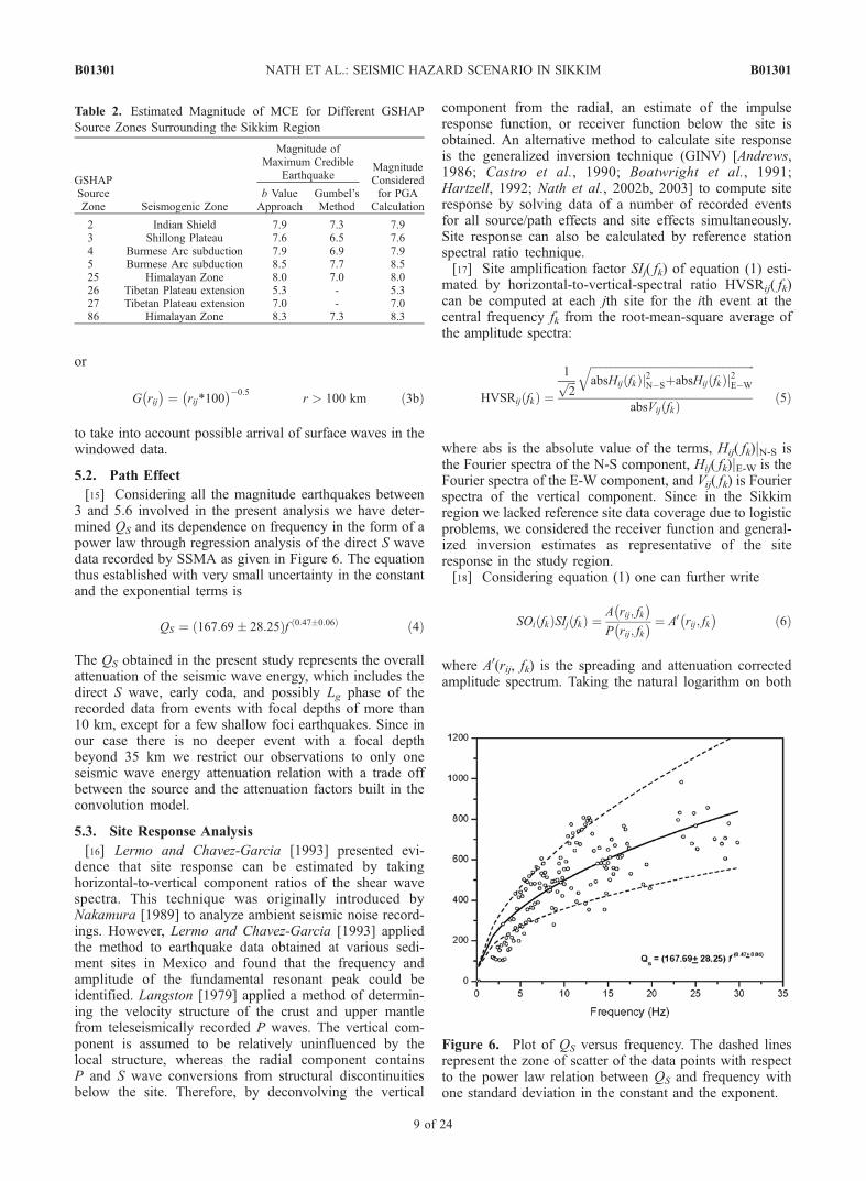
[15] Considering all the magnitude earthquakes between3 and 5.6 involved in the present analysis we have deter-mined QS and its dependence on frequency in the form of apower law through regression analysis of the direct S wavedata recorded by SSMA as given in Figure 6. The equationthus established with very small uncertainty in the constantand the exponential terms is

QS ¼ 167:69� 28:25ð Þf 0:47�0:06ð Þ ð4Þ

The QS obtained in the present study represents the overallattenuation of the seismic wave energy, which includes thedirect S wave, early coda, and possibly Lg phase of therecorded data from events with focal depths of more than10 km, except for a few shallow foci earthquakes. Since inour case there is no deeper event with a focal depthbeyond 35 km we restrict our observations to only oneseismic wave energy attenuation relation with a trade offbetween the source and the attenuation factors built in theconvolution model.

5.3. Site Response Analysis

[16] Lermo and Chavez-Garcia [1993] presented evi-dence that site response can be estimated by takinghorizontal-to-vertical component ratios of the shear wavespectra. This technique was originally introduced byNakamura [1989] to analyze ambient seismic noise record-ings. However, Lermo and Chavez-Garcia [1993] appliedthe method to earthquake data obtained at various sedi-ment sites in Mexico and found that the frequency andamplitude of the fundamental resonant peak could beidentified. Langston [1979] applied a method of determin-ing the velocity structure of the crust and upper mantlefrom teleseismically recorded P waves. The vertical com-ponent is assumed to be relatively uninfluenced by thelocal structure, whereas the radial component containsP and S wave conversions from structural discontinuitiesbelow the site. Therefore, by deconvolving the vertical

component from the radial, an estimate of the impulseresponse function, or receiver function below the site isobtained. An alternative method to calculate site responseis the generalized inversion technique (GINV) [Andrews,1986; Castro et al., 1990; Boatwright et al., 1991;Hartzell, 1992; Nath et al., 2002b, 2003] to compute siteresponse by solving data of a number of recorded eventsfor all source/path effects and site effects simultaneously.Site response can also be calculated by reference stationspectral ratio technique.[17] Site amplification factor SIj( fk) of equation (1) esti-

mated by horizontal-to-vertical-spectral ratio HVSRij( fk)can be computed at each jth site for the ith event at thecentral frequency fk from the root-mean-square average ofthe amplitude spectra:

HVSRij fkð Þ ¼

1ffiffiffi2

pffiffiffiffiffiffiffiffiffiffiffiffiffiffiffiffiffiffiffiffiffiffiffiffiffiffiffiffiffiffiffiffiffiffiffiffiffiffiffiffiffiffiffiffiffiffiffiffiffiffiffiffiffiffiffiffiffiffiffiffiabsHij fkð Þj2N�SþabsHij fkð Þj2E�W

q

absVij fkð Þ ð5Þ

where abs is the absolute value of the terms, Hij( fk)jN-S isthe Fourier spectra of the N-S component, Hij( fk)jE-W is theFourier spectra of the E-W component, and Vij( fk) is Fourierspectra of the vertical component. Since in the Sikkimregion we lacked reference site data coverage due to logisticproblems, we considered the receiver function and general-ized inversion estimates as representative of the siteresponse in the study region.[18] Considering equation (1) one can further write

SOi fkð ÞSIj fkð Þ ¼A rij; fk� �

P rij; fk� � ¼ A0 rij; fk

� �ð6Þ

where A0(rij, fk) is the spreading and attenuation correctedamplitude spectrum. Taking the natural logarithm on both

Table 2. Estimated Magnitude of MCE for Different GSHAP

Source Zones Surrounding the Sikkim Region

GSHAPSourceZone Seismogenic Zone

Magnitude ofMaximum Credible

EarthquakeMagnitudeConsideredfor PGA

Calculationb ValueApproach

Gumbel’sMethod

2 Indian Shield 7.9 7.3 7.93 Shillong Plateau 7.6 6.5 7.64 Burmese Arc subduction 7.9 6.9 7.95 Burmese Arc subduction 8.5 7.7 8.525 Himalayan Zone 8.0 7.0 8.026 Tibetan Plateau extension 5.3 - 5.327 Tibetan Plateau extension 7.0 - 7.086 Himalayan Zone 8.3 7.3 8.3

Figure 6. Plot of QS versus frequency. The dashed linesrepresent the zone of scatter of the data points with respectto the power law relation between QS and frequency withone standard deviation in the constant and the exponent.


9 of 24

B01301

the sides of equation (6) and multiplying by sijk [Hartzell,1992], we can write

Si fkð Þ þ Rj fkð Þ ¼ Dij fkð Þ ð7Þ

where, for the kth frequency fk, Si = sijk lnSOi(fk), Rj =sijk lnSIj(fk) and Dij = sijk lnA0(rij, fk); s is a weightedfactor and an estimate of the standard deviation of thedata given by the ratio of the signal spectrum to a noisesample spectrum, Nij(fk). The algorithm for estimating stried in this analysis is

sijk ¼ max min A rij; fk� �

=N rij; fk� �

; 5:0� �

; 1:0

=5:0 ð8Þ

where s is normalized and limited to the range of 1.0 to0.2. This imposes a balance in the quality of the data withthe need to include as many observations as possible toaverage out radiation pattern and source directivity effects.Nij(fk) is obtained from a 2.0 s or less duration noisesample immediately preceding the shear wave arrival.Equation (7) is written in the matrix form following thenotation of Menke [1989] and solved by generalizedinversion scheme using singular value decomposition[Nath et al., 2002b] for computing the site response. Themethod requires a reference site with known responsevalue in the frequency range of interest to minimize thetrade-off between the source and site parameter values asobserved by Andrews [1986]. In the present study, in theabsence of a reference site, we consider GINV results to bean average site response spectral function estimating thepattern of site amplification variation at different frequen-cies, whereas HVSR represents the true nonreference sitespectral amplification.[19] Station site amplification has been computed from

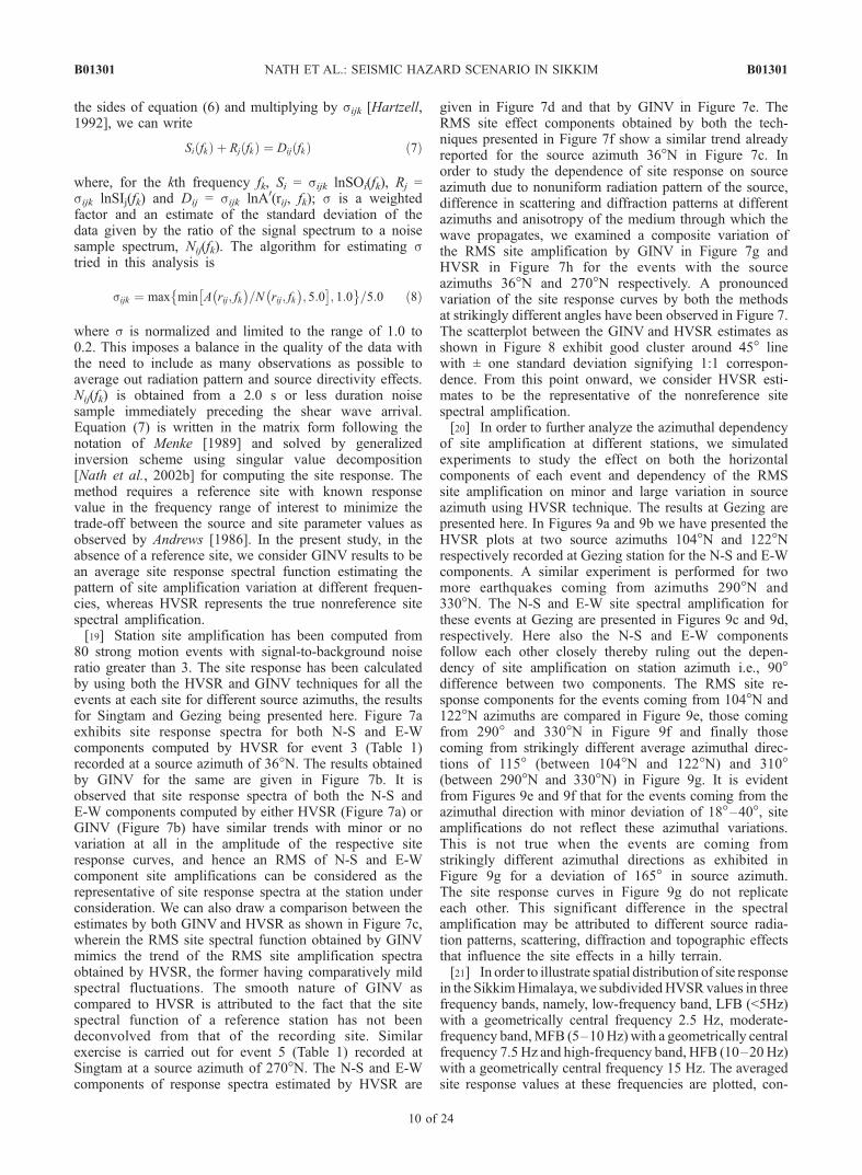
80 strong motion events with signal-to-background noiseratio greater than 3. The site response has been calculatedby using both the HVSR and GINV techniques for all theevents at each site for different source azimuths, the resultsfor Singtam and Gezing being presented here. Figure 7aexhibits site response spectra for both N-S and E-Wcomponents computed by HVSR for event 3 (Table 1)recorded at a source azimuth of 36�N. The results obtainedby GINV for the same are given in Figure 7b. It isobserved that site response spectra of both the N-S andE-W components computed by either HVSR (Figure 7a) orGINV (Figure 7b) have similar trends with minor or novariation at all in the amplitude of the respective siteresponse curves, and hence an RMS of N-S and E-Wcomponent site amplifications can be considered as therepresentative of site response spectra at the station underconsideration. We can also draw a comparison between theestimates by both GINV and HVSR as shown in Figure 7c,wherein the RMS site spectral function obtained by GINVmimics the trend of the RMS site amplification spectraobtained by HVSR, the former having comparatively mildspectral fluctuations. The smooth nature of GINV ascompared to HVSR is attributed to the fact that the sitespectral function of a reference station has not beendeconvolved from that of the recording site. Similarexercise is carried out for event 5 (Table 1) recorded atSingtam at a source azimuth of 270�N. The N-S and E-Wcomponents of response spectra estimated by HVSR are

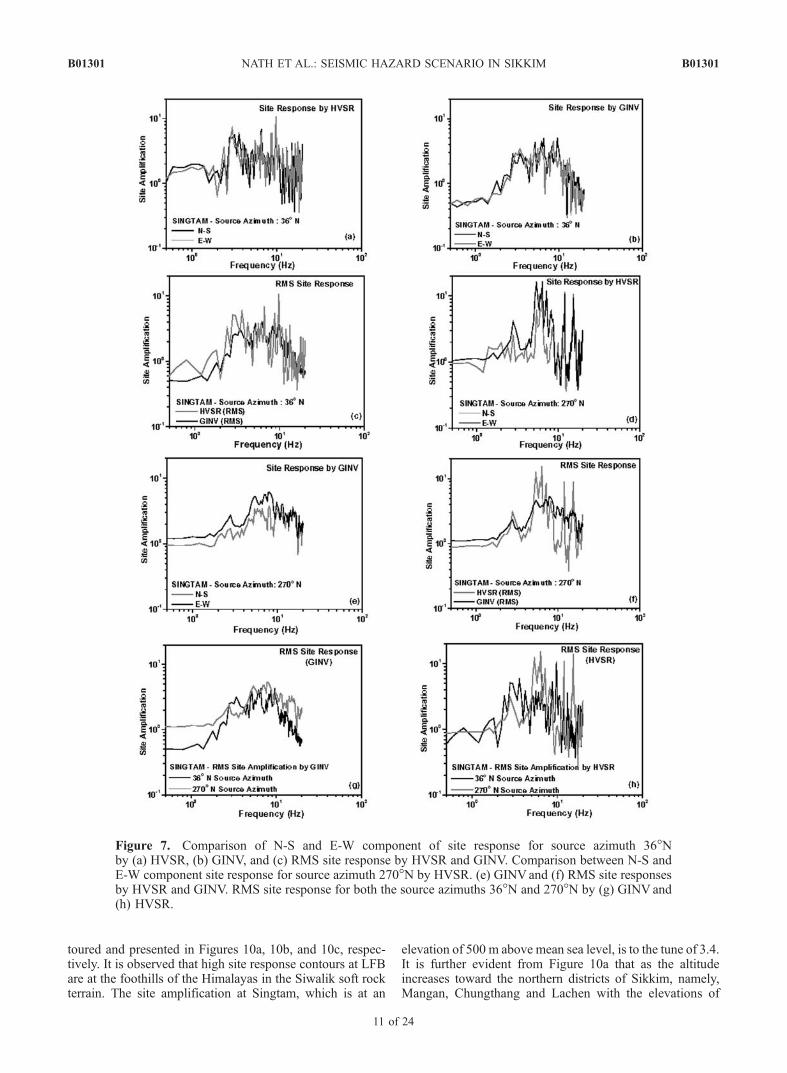
given in Figure 7d and that by GINV in Figure 7e. TheRMS site effect components obtained by both the tech-niques presented in Figure 7f show a similar trend alreadyreported for the source azimuth 36�N in Figure 7c. Inorder to study the dependence of site response on sourceazimuth due to nonuniform radiation pattern of the source,difference in scattering and diffraction patterns at differentazimuths and anisotropy of the medium through which thewave propagates, we examined a composite variation ofthe RMS site amplification by GINV in Figure 7g andHVSR in Figure 7h for the events with the sourceazimuths 36�N and 270�N respectively. A pronouncedvariation of the site response curves by both the methodsat strikingly different angles have been observed in Figure 7.The scatterplot between the GINV and HVSR estimates asshown in Figure 8 exhibit good cluster around 45� linewith ± one standard deviation signifying 1:1 correspon-dence. From this point onward, we consider HVSR esti-mates to be the representative of the nonreference sitespectral amplification.[20] In order to further analyze the azimuthal dependency

of site amplification at different stations, we simulatedexperiments to study the effect on both the horizontalcomponents of each event and dependency of the RMSsite amplification on minor and large variation in sourceazimuth using HVSR technique. The results at Gezing arepresented here. In Figures 9a and 9b we have presented theHVSR plots at two source azimuths 104�N and 122�Nrespectively recorded at Gezing station for the N-S and E-Wcomponents. A similar experiment is performed for twomore earthquakes coming from azimuths 290�N and330�N. The N-S and E-W site spectral amplification forthese events at Gezing are presented in Figures 9c and 9d,respectively. Here also the N-S and E-W componentsfollow each other closely thereby ruling out the depen-dency of site amplification on station azimuth i.e., 90�difference between two components. The RMS site re-sponse components for the events coming from 104�N and122�N azimuths are compared in Figure 9e, those comingfrom 290� and 330�N in Figure 9f and finally thosecoming from strikingly different average azimuthal direc-tions of 115� (between 104�N and 122�N) and 310�(between 290�N and 330�N) in Figure 9g. It is evidentfrom Figures 9e and 9f that for the events coming from theazimuthal direction with minor deviation of 18�–40�, siteamplifications do not reflect these azimuthal variations.This is not true when the events are coming fromstrikingly different azimuthal directions as exhibited inFigure 9g for a deviation of 165� in source azimuth.The site response curves in Figure 9g do not replicateeach other. This significant difference in the spectralamplification may be attributed to different source radia-tion patterns, scattering, diffraction and topographic effectsthat influence the site effects in a hilly terrain.[21] In order to illustrate spatial distribution of site response

in the SikkimHimalaya, we subdividedHVSR values in threefrequency bands, namely, low-frequency band, LFB (<5Hz)with a geometrically central frequency 2.5 Hz, moderate-frequency band,MFB (5–10Hz) with a geometrically centralfrequency 7.5Hz and high-frequency band, HFB (10–20Hz)with a geometrically central frequency 15 Hz. The averagedsite response values at these frequencies are plotted, con-


10 of 24

B01301

toured and presented in Figures 10a, 10b, and 10c, respec-tively. It is observed that high site response contours at LFBare at the foothills of the Himalayas in the Siwalik soft rockterrain. The site amplification at Singtam, which is at an

elevation of 500 m above mean sea level, is to the tune of 3.4.It is further evident from Figure 10a that as the altitudeincreases toward the northern districts of Sikkim, namely,Mangan, Chungthang and Lachen with the elevations of

Figure 7. Comparison of N-S and E-W component of site response for source azimuth 36�Nby (a) HVSR, (b) GINV, and (c) RMS site response by HVSR and GINV. Comparison between N-S andE-W component site response for source azimuth 270�N by HVSR. (e) GINVand (f) RMS site responsesby HVSR and GINV. RMS site response for both the source azimuths 36�N and 270�N by (g) GINV and(h) HVSR.


11 of 24

B01301

1000, 2200 and 3800 m, respectively, the site responsediminishes at 2.5 Hz. For the MFB with the geometricallycentral frequency of 7.5 Hz we observe in Figure 10b adifferent scenario of spatial variation of site amplification incontrast to that at low-frequency band. Here, the higherHVSR values peak near Mangan at an elevation of 1000 m.In this region, the hillslope is much steeper, the maximum siteamplification observed in this case is 4.6. In the HFB withgeometrically central frequency 15 Hz, the spatial variationpattern (Figure 10c) of site amplification shifts further north-east toward Chungthang with an altitude of 2200 m, siteresponse peaking to a value of 5.8 on the high hill scarpbetween Mangan and Chungthang. It is to be noted that theGangtok lineament passes very close to Chungthang and isseismogenic in the area. This side of the hill is also very steep,thereby contributing to the diffraction wave trains in the codapart of the S wave. This variation in the SR contourpattern at three distinct frequency bands seems to followthe topography for the moderate- to high-frequency re-gime and is consistent with the findings of Bouchon andBarker [1996], when they simulated an experiment toobserve ground motion amplification at or near the top ofthe hill depending on the slope and the resonance frequencyof the respective morphometric signature of the terrain. Eventhe experiment simulated by Pedersen et al. [1994] showsthat the level of amplification can be significantly higherexceeding a factor of 10 at the slopes and base of themountain as a function of frequency. In our case, we seethe amplification variation from low- to high-frequencybands at different topographic platforms with low to higherresonance frequency in line with the works of Bouchon andBarker [1996] and Pedersen et al. [1994].

5.4. Source Spectra and Simulation of SpectralAcceleration

[22] Since we have estimated propagation path term P(rij,fk), and site effect term SIj(fk) for equation (1), our task willnow be to determine source term SOi(fk). The sourcespectral function SOi(fk) of the ith event used in this studyis the acceleration source spectrum defined as the Brune’ssource model [Dutta et al., 2003; Hwang and Huo, 1997],

alternately termed as omega (wk = 2pfk) squared circularcrack source model [Brune, 1970], given as

SOi fkð Þ ¼RqfF 2pfkð Þ2h i

ffiffiffi2

p4prb3� � _Moi fkð Þ ð9Þ

where Rqf(=0.63) is the radiation pattern averaged over anappropriate range of azimuths and takeoff angles, F(=2.0)accounts for the amplification of the seismic wave at thefree surface, r is the crustal density of the continental crustat the focal depth, b is the shear wave velocity at the sourceregion and _Moi(fk) is the moment rate spectrum. The factorffiffiffi2

paccounts for the partition of S wave energy into

transverse components. We have assumed r to be equal to2.7 g/cm3 (crustal density) and b = 4.0 km/s [De, 2000]. Themoment rate spectrum _Moi(fk) can be expressed as

_Moi fkð Þ ¼ Moi

1þ fk=fcið Þgi ð10Þ

where Moi, fci, and gi respectively are the scalar moment,corner frequency and the high-frequency spectral fall-offassociated with the ith earthquake. Substituting this inequation (9), we get

SOi fkð Þ ¼RqfF 2pfkð Þ2

h iffiffiffi2

p4prb3� � Moi

1þ fk=fcið Þgi ð11Þ

Since Moi, fci and gi control the Brune’s source model, wefix up the initial values for these parameters. We initializeMoi by computing the value of M0 for a given MW usingKanamori’s relation [Hanks and Kanamori, 1979], which isgiven as,

MW ¼ 2=3 log M0ð Þ � 10:73 ð12Þ

(M0 in dyn cm). The initial values of fci and gi are assumed tobe 0.1 Hz [Dutta et al., 2003] and 2 [Hwang and Huo, 1997],respectively. Estimation of these values is carried out in aniterative fashion. Iteration continues until the differencebetween the observed and the simulated source spectra tendsto approach a minimum value. This exercise was carried outfor more than 25 events. In most of the cases we obtainedconvergence and hence the best fit solution. However, insome, where convergence was not achieved, we have takenthe results yielded at the last step of iteration [Dutta et al.,2003]. The values of gi for the analyzed events as obtainedfrom above stated procedure vary from 1.6 to 2.4. Using theBrune’s model of equation (9) the source spectra has beenestimated and compared with the deconvolved source spectrafrom the observed data at all the recording stations in theSikkimHimalaya. The simulatedmoment rate spectra and thespectral acceleration have also been compared with thoseextracted from observed data at the respective stations. Thesite response, source spectra, moment rate spectra and thespectral acceleration for the recording station Singtam,Gezing, Mangan and the state capital Gangtok are presentedin Figures 11, 12, 13, and 14 respectively. At Singtam inFigure 11, the source spectra have been computed for theevent coming at an azimuthal direction of 270�N. The

Figure 8. Scatterplot between HVSR and GINV depictingdata clustering around the 45� 1:1 correspondence line.


12 of 24

B01301

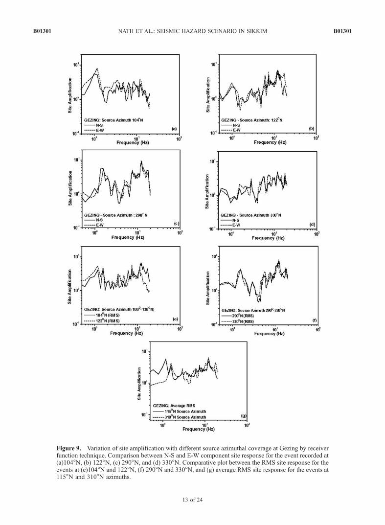
Figure 9. Variation of site amplification with different source azimuthal coverage at Gezing by receiverfunction technique. Comparison between N-S and E-W component site response for the event recorded at(a)104�N, (b) 122�N, (c) 290�N, and (d) 330�N. Comparative plot between the RMS site response for theevents at (e)104�N and 122�N, (f) 290�N and 330�N, and (g) average RMS site response for the events at115�N and 310�N azimuths.


13 of 24

B01301

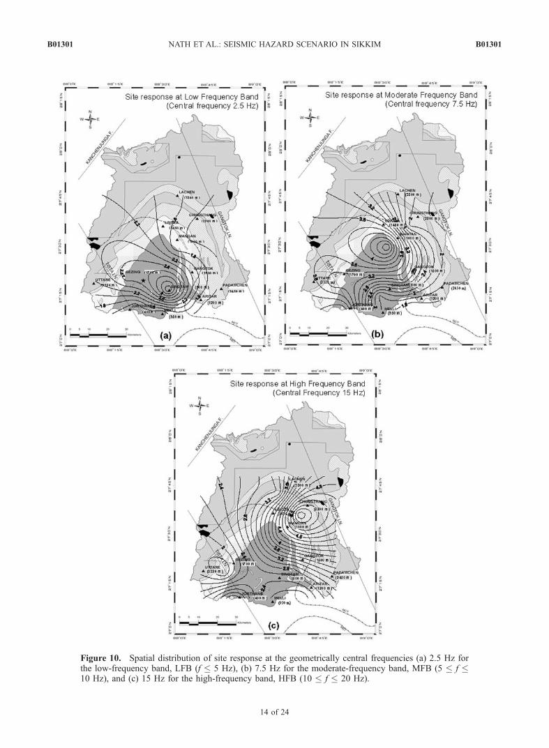
Figure 10. Spatial distribution of site response at the geometrically central frequencies (a) 2.5 Hz forthe low-frequency band, LFB (f � 5 Hz), (b) 7.5 Hz for the moderate-frequency band, MFB (5 � f �10 Hz), and (c) 15 Hz for the high-frequency band, HFB (10 � f � 20 Hz).


14 of 24

B01301

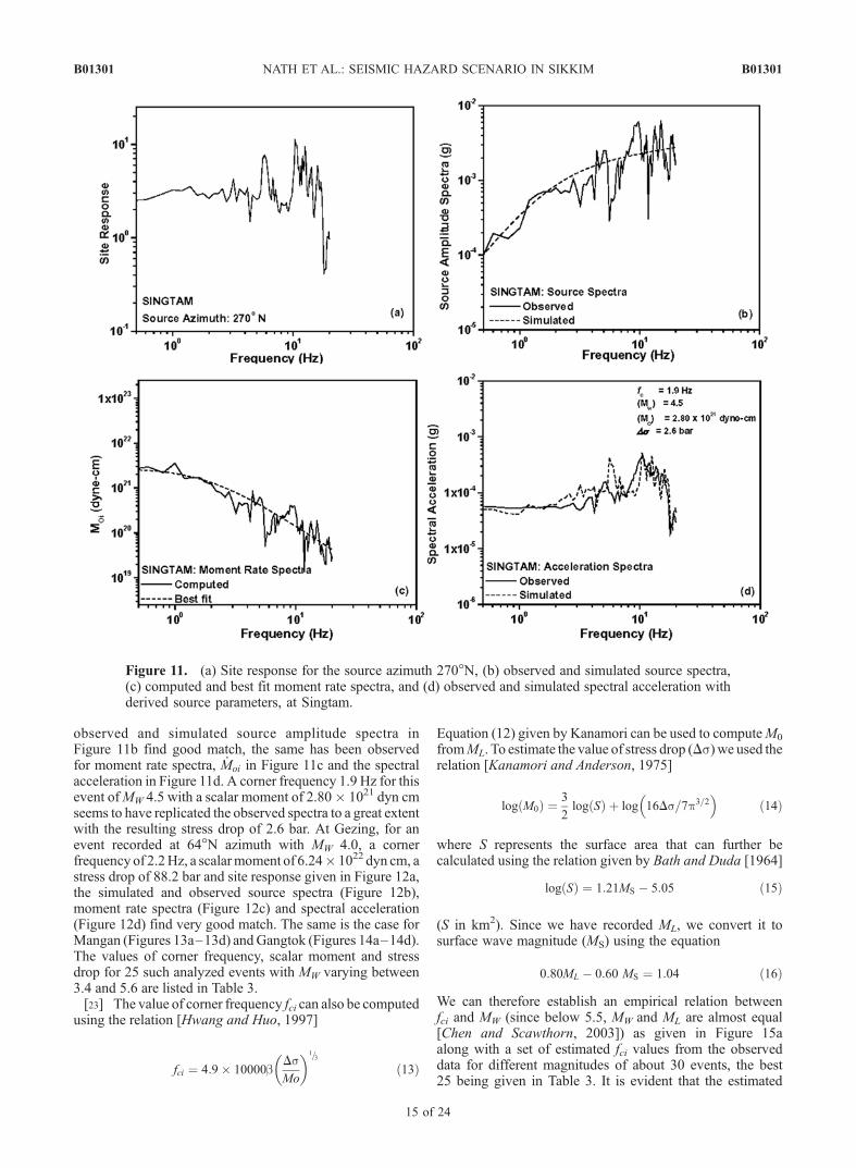
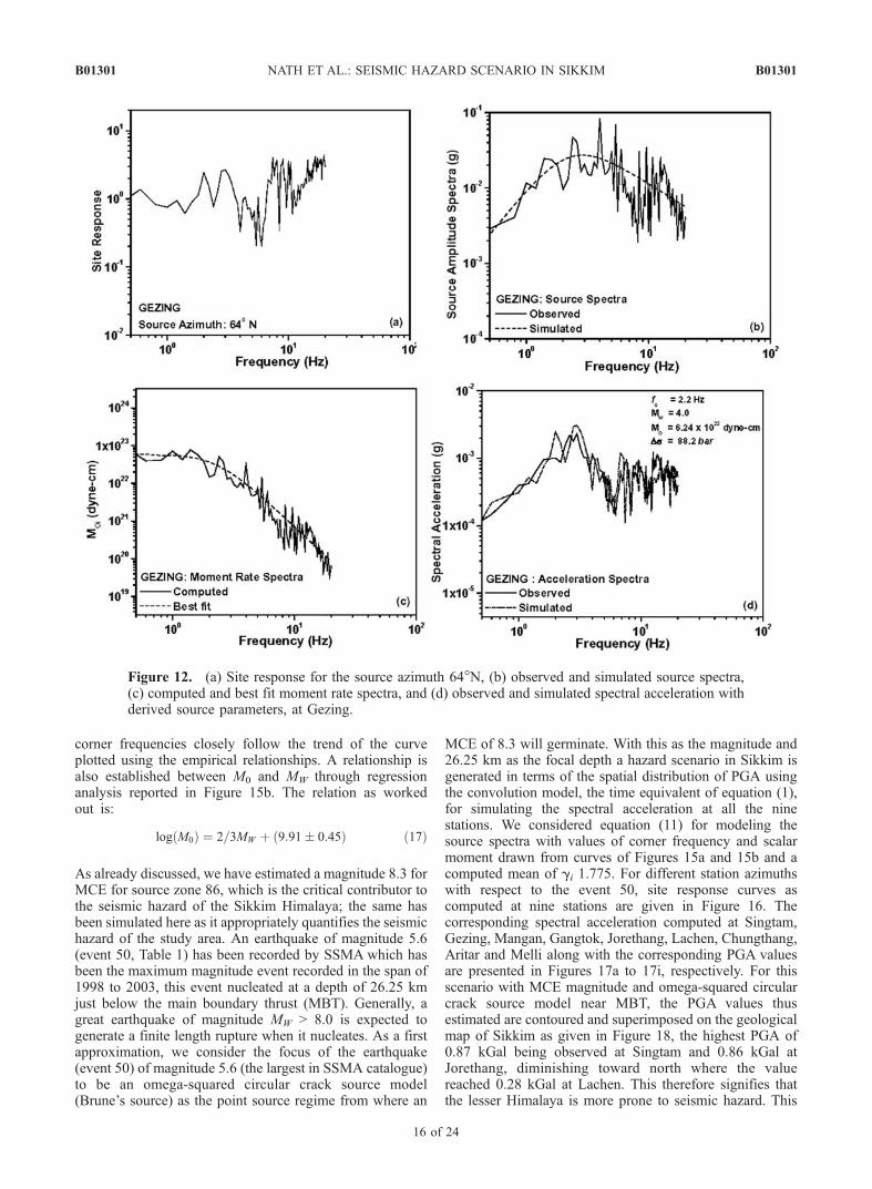
observed and simulated source amplitude spectra inFigure 11b find good match, the same has been observedfor moment rate spectra, _Moi in Figure 11c and the spectralacceleration in Figure 11d. A corner frequency 1.9 Hz for thisevent ofMW 4.5 with a scalar moment of 2.80 1021 dyn cmseems to have replicated the observed spectra to a great extentwith the resulting stress drop of 2.6 bar. At Gezing, for anevent recorded at 64�N azimuth with MW 4.0, a cornerfrequency of 2.2Hz, a scalarmoment of 6.24 1022 dyn cm, astress drop of 88.2 bar and site response given in Figure 12a,the simulated and observed source spectra (Figure 12b),moment rate spectra (Figure 12c) and spectral acceleration(Figure 12d) find very good match. The same is the case forMangan (Figures 13a–13d) andGangtok (Figures 14a–14d).The values of corner frequency, scalar moment and stressdrop for 25 such analyzed events with MW varying between3.4 and 5.6 are listed in Table 3.[23] The value of corner frequency fci can also be computed

using the relation [Hwang and Huo, 1997]

fci ¼ 4:9 10000bDsMo

�1=3

ð13Þ

Equation (12) given by Kanamori can be used to computeM0

fromML. To estimate the value of stress drop (Ds) we used therelation [Kanamori and Anderson, 1975]

log M0ð Þ ¼ 3

2log Sð Þ þ log 16Ds=7p3=2

� �ð14Þ

where S represents the surface area that can further becalculated using the relation given by Bath and Duda [1964]

log Sð Þ ¼ 1:21MS � 5:05 ð15Þ

(S in km2). Since we have recorded ML, we convert it tosurface wave magnitude (MS) using the equation

0:80ML � 0:60 MS ¼ 1:04 ð16Þ

We can therefore establish an empirical relation betweenfci and MW (since below 5.5, MW and ML are almost equal[Chen and Scawthorn, 2003]) as given in Figure 15aalong with a set of estimated fci values from the observeddata for different magnitudes of about 30 events, the best25 being given in Table 3. It is evident that the estimated

Figure 11. (a) Site response for the source azimuth 270�N, (b) observed and simulated source spectra,(c) computed and best fit moment rate spectra, and (d) observed and simulated spectral acceleration withderived source parameters, at Singtam.


15 of 24

B01301

corner frequencies closely follow the trend of the curveplotted using the empirical relationships. A relationship isalso established between M0 and MW through regressionanalysis reported in Figure 15b. The relation as workedout is:

log M0ð Þ ¼ 2=3MW þ 9:91� 0:45ð Þ ð17Þ

As already discussed, we have estimated a magnitude 8.3 forMCE for source zone 86, which is the critical contributor tothe seismic hazard of the Sikkim Himalaya; the same hasbeen simulated here as it appropriately quantifies the seismichazard of the study area. An earthquake of magnitude 5.6(event 50, Table 1) has been recorded by SSMA which hasbeen the maximum magnitude event recorded in the span of1998 to 2003, this event nucleated at a depth of 26.25 kmjust below the main boundary thrust (MBT). Generally, agreat earthquake of magnitude MW > 8.0 is expected togenerate a finite length rupture when it nucleates. As a firstapproximation, we consider the focus of the earthquake(event 50) of magnitude 5.6 (the largest in SSMA catalogue)to be an omega-squared circular crack source model(Brune’s source) as the point source regime from where an

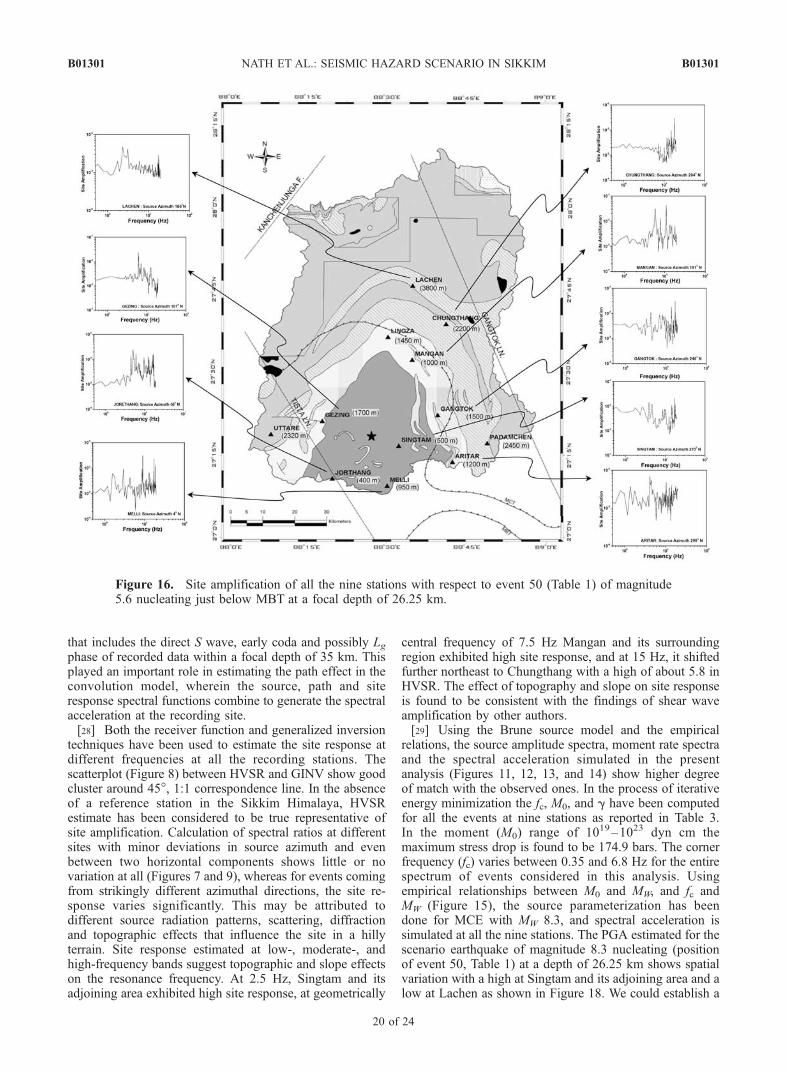
MCE of 8.3 will germinate. With this as the magnitude and26.25 km as the focal depth a hazard scenario in Sikkim isgenerated in terms of the spatial distribution of PGA usingthe convolution model, the time equivalent of equation (1),for simulating the spectral acceleration at all the ninestations. We considered equation (11) for modeling thesource spectra with values of corner frequency and scalarmoment drawn from curves of Figures 15a and 15b and acomputed mean of gi 1.775. For different station azimuthswith respect to the event 50, site response curves ascomputed at nine stations are given in Figure 16. Thecorresponding spectral acceleration computed at Singtam,Gezing, Mangan, Gangtok, Jorethang, Lachen, Chungthang,Aritar and Melli along with the corresponding PGA valuesare presented in Figures 17a to 17i, respectively. For thisscenario with MCE magnitude and omega-squared circularcrack source model near MBT, the PGA values thusestimated are contoured and superimposed on the geologicalmap of Sikkim as given in Figure 18, the highest PGA of0.87 kGal being observed at Singtam and 0.86 kGal atJorethang, diminishing toward north where the valuereached 0.28 kGal at Lachen. This therefore signifies thatthe lesser Himalaya is more prone to seismic hazard. This

Figure 12. (a) Site response for the source azimuth 64�N, (b) observed and simulated source spectra,(c) computed and best fit moment rate spectra, and (d) observed and simulated spectral acceleration withderived source parameters, at Gezing.


16 of 24

B01301

aspect is further analyzed through attenuation study fromstrong motion accelerometric data.

6. Attenuation Law in the Sikkim Himalaya

[24] An evaluation of seismic hazard requires an estimateof expected ground motion at the site of interest. The mostcommon means of estimating ground motion in engineeringpractice is the use of an attenuation relationship. Anattenuation relation can be described by its more commonlogarithmic form [Chen and Scawthorn, 2003] as

ln Yð Þ ¼ C1 þ C2 M � C3 ln rð Þ � C4 r þ C5 F þ C6 S þ e ð18Þ

where Y is the strong motion parameter of interest (PGA inour case), M is earthquake magnitude, r is a measure ofsource-to-site distance, F is a parameter characterizing typeof faulting, S is the parameter characterizing local sitecondition, and e is the random error term. Ignoring the site,topography, and fault parameter, the generalized attenuationlaw takes the form

ln Yð Þ ¼ C1 þ C2 M � C3 ln rð Þ � C4 r ð19Þ

We have used a semiempirical approach by selecting tominimize the difference between observed and estimatedvalues of ground motion and obtained the followingattenuation law:

ln Yð Þ ¼ �3:6þ 0:72M � 1:08 ln r þ 0:007r ð20Þ

Equation (20) is the first-order attenuation law for theSikkim Himalaya. This is a mean attenuation relationshipwithout considering local site conditions and for hypo-central distances less than 100 km. A comparative plotbetween our first-order relationship, Joyner and Boore’s[1981, 1988] relationship, Campbell’s [1988] relation andFukushima and Tanaka [1990] relationship for MW = 7and varying hypocentral distances from 0 to 100 km isshown in Figure 19. Our first-order relation fits well into thisset of attenuation laws. Since we have used a functional formto start with, which has a theoretical basis, the attenuationrelation is expected to be more realistic devoid of local siteconditions. Since we have already observed in our previousanalysis that the spectral acceleration depends on siteamplification, topography, the source azimuth and the local

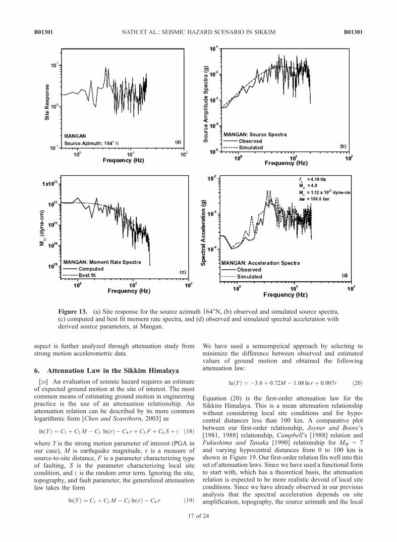
Figure 13. (a) Site response for the source azimuth 164�N, (b) observed and simulated source spectra,(c) computed and best fit moment rate spectra, and (d) observed and simulated spectral acceleration withderived source parameters, at Mangan.


17 of 24

B01301

site conditions, it became necessary for us to work out a localattenuation relation by modifying our first-order attenuationlaw.[25] We started with the general form of equation given

by Campbell’s attenuation law for spectral acceleration as[Campbell, 1997]

ln SAHð Þ ¼ ln AHð Þ þ c1 þ c2 tanh c3 M � 4:7ð Þ½ � þ c4 þ c5Mð Þrþ 0:5c6SSR þ c7 tanh c8Dð Þ 1� SHRð Þ þ fSA Dð Þ þ e

ð21Þ

where SAH is the horizontal spectral acceleration, AH is thehorizontal PGA, SSR and SHR are variables representinglocal site conditions for soft rock and hard rock,respectively, D is the depth to the basement rock, and fSAis a function of D.[26] Since in our study region, the sediment cover is very

thin, we neglected the terms relating to hard rock and softrock; instead we introduced a term of site amplification totake into account local site conditions. Moreover, beingsituated in a hilly terrain, dependence on topography is

expected, and to account for this, we have introduced a termfor station elevation. Our established second-order attenua-tion relation therefore takes the following shape:

ln PGAð Þ ¼ ln SAð Þ � a1� a2þ a3 Mð Þr � a4 h� a5 ln SRð Þð22Þ

where h is the site elevation, SR the site response, and SA isthe spectral acceleration at respective frequencies for whichthe relation holds well. A set of spectral attenuationrelations has been determined at different source azimuthsas given in Table 4. It is to be noted that due to the paucityof data within the magnitude range 5.6 to 8.5 we simulatedthe spectral acceleration at these magnitudes and clubbed itwith the recorded spectra. This relation therefore uses boththe recorded and simulated events, with local site conditionsincorporated in the simulation. As shown in Table 4 forgeometrically central frequencies 2.5, 7.5 and 15 Hzrepresenting the already discussed LFB, MFB and HFBfrequency regimes, the difference in values of respectivecoefficients for different azimuths is not conspicuous. As

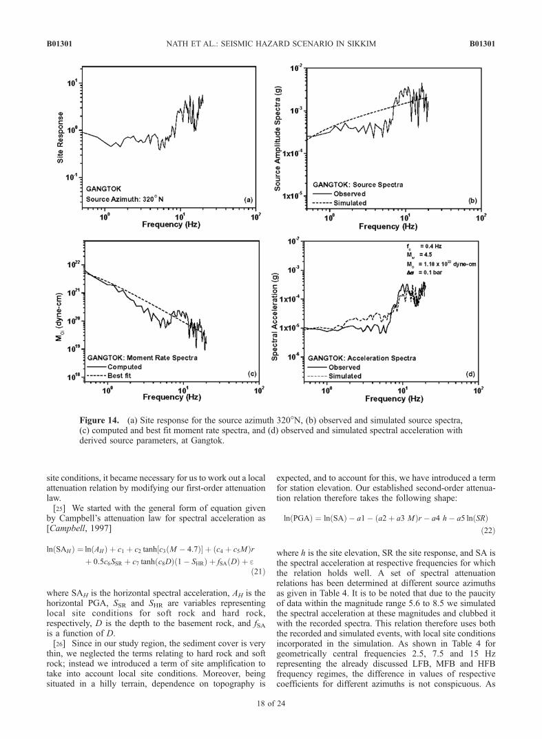
Figure 14. (a) Site response for the source azimuth 320�N, (b) observed and simulated source spectra,(c) computed and best fit moment rate spectra, and (d) observed and simulated spectral acceleration withderived source parameters, at Gangtok.


18 of 24

B01301

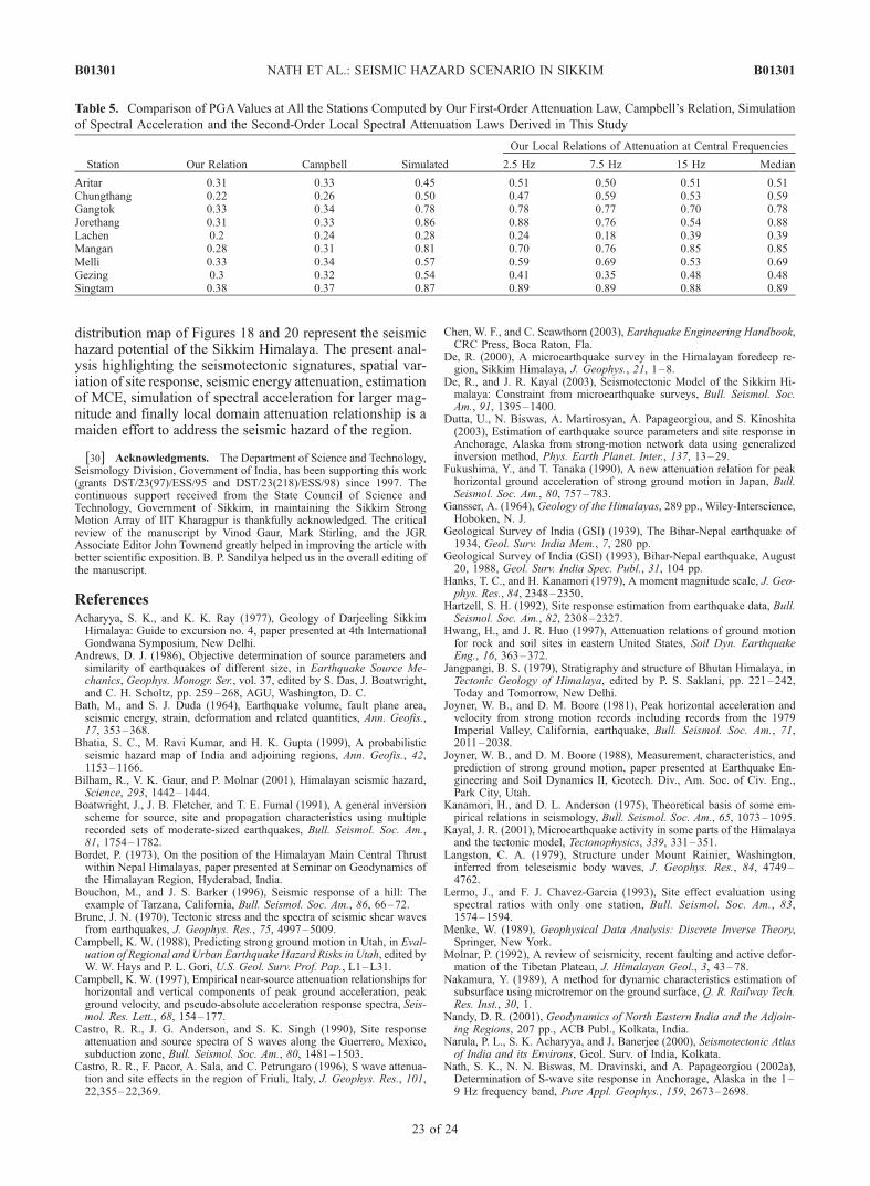
expected, the site amplification and spectral accelerationbalance the azimuthal changes in the attenuation relations,thereby, largely stabilizing the coefficients. We thereforehave a composite relation for each of the three centralfrequencies. Using this set of attenuation laws, wecomputed the PGA for the scenario earthquake justdiscussed. The median PGA contour map constructed andpresented in Figure 20 from the attenuation laws showsa similar trend in the spatial distribution, the highest of0.89 kGal being observed at Singtam, 0.88 kGal atJorethang and 0.85 kGal at Mangan. The value diminishestoward north as is also observed in Figure 18. A comparisonbetween PGA computed by our first-order attenuation law,Campbell’s relation, simulation, second-order spectralattenuation relation at different central frequencies and themedian is presented in Table 5. Since our first-order relationand that of Campbell do not consider the local siteconditions, the estimated PGA values were found verylow. The PGA estimated through simulation and spectralattenuation relations closely follow each other, both beingconsistent with the occurrence of a scenario earthquake ofgreat magnitude in the Sikkim region.

7. Summary and Conclusions

[27] The Darjeeling-Sikkim Himalayas are well known tobe seismically active. The strong motion recordings anddepth profile in the SikkimHimalaya are shown in Figures 3aand 3b. The composite fault plane solution from the strongmotion events suggests thrust faulting with strike slipcomponent along MBT. Global Seismic Hazard AssessmentProgram also characterized Sikkim region as surrounded by8 seismic source zones, established in the present study asthe potential seismogenic zones, of which the Himalayanbelt comprising GSHAP sources 25 and 86 is the critical

contributor to the seismic hazard potential of the region. Themagnitude of MCE by b value approach for the Sikkimregion is estimated to be 8.3 (Figure 5 and Table 2) with10% probability of exceedance in 50 years using the ISCcatalogue of 35 years. Considering the widespread damagescaused in the state capital of Sikkim due to earthquakes of1934 (MW 8) and 1988 (MW 7.2), a 50-year estimationseemed reasonable, fixing a return period of 475 years. Ofthe 150 earthquakes recorded by SSMA in a span of 5 years(1998–2003) the highest-magnitude MW of 5.6 has beenrecorded for an event (event 50, Table 1) that nucleated at afocal depth of 26.25 km just below MBT. The S wave Qfactor has been determined as a function of frequency in theform of a power law (Figure 6) using 80 well-recordedstrong motion events (Table 1). The seismic energy atten-uation law is considered to represent an overall attenuation

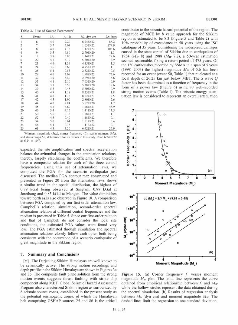
Table 3. List of Source Parametersa

Sl Event Mw fc, Hz M0, dyn cm Ds, bars

1 6 4.0 2.20 6.24E+22 88.22 7 3.7 5.04 1.03E+22 174.93 8 4.0 4.18 1.12E+22 108.64 9 3.5 6.80 2.70E+20 11.35 12 3.8 5.80 1.14E+21 29.66 22 4.3 3.70 5.80E+20 3.97 23 4.6 1.39 4.15E+21 1.58 24 3.6 5.60 4.75E+19 1.19 25 5.1 0.53 2.32E+22 0.510 29 4.6 3.09 1.98E+22 77.611 32 3.9 5.40 2.69E+20 5.612 33 4.1 2.10 7.03E+20 0.913 34 3.7 6.50 5.38E+20 19.614 39 5.3 0.48 5.80E+22 0.915 40 4.9 1.18 8.23E+21 1.816 41 4.8 1.33 8.02E+21 2.517 42 4.5 1.90 2.80E+21 2.618 44 4.0 2.84 5.62E+20 1.719 45 4.3 6.60 1.28E+21 48.920 46 3.4 4.16 1.41E+21 13.521 50 5.6 0.35 1.88E+23 1.122 52 4.5 0.40 1.18E+22 0.123 54 5.0 0.64 1.01E+22 0.424 56 5.1 0.38 1.11E+22 0.125 61 4.3 3.20 6.42E+21 27.9

aMoment magnitude (MW), corner frequency (fc), scalar moment (M0),and stress drop (Ds) determined for 25 events in this study. Read 6.24E+22as 6.24 1022.

Figure 15. (a) Corner frequency fc verses momentmagnitude MW plot. The solid line represents the curveobtained from empirical relationship between fc and MW

while the hollow circles represent the data obtained duringthe spectral simulation. (b) Results of regression analysisbetween M0 (dyn cm) and moment magnitude MW. Thedashed lines limit the regression to one standard deviation.


19 of 24

B01301

that includes the direct S wave, early coda and possibly Lgphase of recorded data within a focal depth of 35 km. Thisplayed an important role in estimating the path effect in theconvolution model, wherein the source, path and siteresponse spectral functions combine to generate the spectralacceleration at the recording site.[28] Both the receiver function and generalized inversion

techniques have been used to estimate the site response atdifferent frequencies at all the recording stations. Thescatterplot (Figure 8) between HVSR and GINV show goodcluster around 45�, 1:1 correspondence line. In the absenceof a reference station in the Sikkim Himalaya, HVSRestimate has been considered to be true representative ofsite amplification. Calculation of spectral ratios at differentsites with minor deviations in source azimuth and evenbetween two horizontal components shows little or novariation at all (Figures 7 and 9), whereas for events comingfrom strikingly different azimuthal directions, the site re-sponse varies significantly. This may be attributed todifferent source radiation patterns, scattering, diffractionand topographic effects that influence the site in a hillyterrain. Site response estimated at low-, moderate-, andhigh-frequency bands suggest topographic and slope effectson the resonance frequency. At 2.5 Hz, Singtam and itsadjoining area exhibited high site response, at geometrically

central frequency of 7.5 Hz Mangan and its surroundingregion exhibited high site response, and at 15 Hz, it shiftedfurther northeast to Chungthang with a high of about 5.8 inHVSR. The effect of topography and slope on site responseis found to be consistent with the findings of shear waveamplification by other authors.[29] Using the Brune source model and the empirical

relations, the source amplitude spectra, moment rate spectraand the spectral acceleration simulated in the presentanalysis (Figures 11, 12, 13, and 14) show higher degreeof match with the observed ones. In the process of iterativeenergy minimization the fc, M0, and g have been computedfor all the events at nine stations as reported in Table 3.In the moment (M0) range of 1019–1023 dyn cm themaximum stress drop is found to be 174.9 bars. The cornerfrequency (fc) varies between 0.35 and 6.8 Hz for the entirespectrum of events considered in this analysis. Usingempirical relationships between M0 and MW, and fc andMW (Figure 15), the source parameterization has beendone for MCE with MW 8.3, and spectral acceleration issimulated at all the nine stations. The PGA estimated for thescenario earthquake of magnitude 8.3 nucleating (positionof event 50, Table 1) at a depth of 26.25 km shows spatialvariation with a high at Singtam and its adjoining area and alow at Lachen as shown in Figure 18. We could establish a

Figure 16. Site amplification of all the nine stations with respect to event 50 (Table 1) of magnitude5.6 nucleating just below MBT at a focal depth of 26.25 km.


20 of 24

B01301

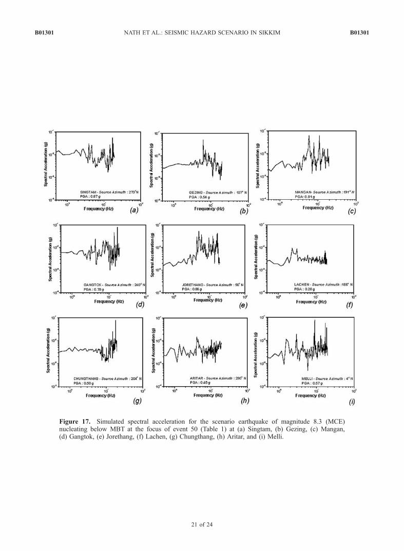
Figure 17. Simulated spectral acceleration for the scenario earthquake of magnitude 8.3 (MCE)nucleating below MBT at the focus of event 50 (Table 1) at (a) Singtam, (b) Gezing, (c) Mangan,(d) Gangtok, (e) Jorethang, (f) Lachen, (g) Chungthang, (h) Aritar, and (i) Melli.


21 of 24

B01301

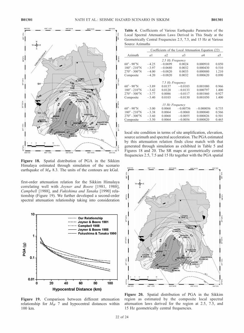
first-order attenuation relation for the Sikkim Himalayacorrelating well with Joyner and Boore [1981, 1988],Campbell [1988], and Fukishima and Tanaka [1990] rela-tionship (Figure 19). We further developed a second-orderspectral attenuation relationship taking into consideration

local site condition in terms of site amplification, elevation,source azimuth and spectral acceleration. The PGA estimatedby this attenuation relation finds close match with thatgenerated through simulation as exhibited in Table 5 andFigures 18 and 20. The SR maps at geometrically centralfrequencies 2.5, 7.5 and 15 Hz together with the PGA spatial

Figure 18. Spatial distribution of PGA in the SikkimHimalaya estimated through simulation of the scenarioearthquake of MW 8.3. The units of the contours are kGal.

Figure 19. Comparison between different attenuationrelationship for MW 7 and hypocentral distances within100 km.

Table 4. Coefficients of Various Earthquake Parameters of the

Local Spectral Attenuation Laws Derived in This Study at the

Geometrically Central Frequencies 2.5, 7.5, and 15 Hz at Various

Source Azimuths

Azimuth

Coefficients of the Local Attenuation Equation (22)

a1 a2 a3 a4 a5

2.5 Hz Frequency60�–90�N �4.25 �0.0699 0.0024 0.000910 0.850180�–210�N �3.97 �0.0680 0.0032 0.000430 0.510270�–300�N �4.00 �0.0820 0.0033 0.000880 1.210Composite �4.20 �0.0820 0.0032 0.000620 0.890

7.5 Hz Frequency60�–90�N �3.89 0.0137 �0.0103 0.001080 0.966180�–210�N �3.42 0.0120 �0.0133 0.000797 1.400270�–300�N �3.77 0.0086 �0.0117 0.001860 0.927Composite �3.40 0.0103 �0.0130 0.001050 1.400

15 Hz Frequency60�–90�N �3.00 0.0068 �0.00756 �0.000056 0.735180�–210�N �3.38 0.0064 �0.0060 0.000040 0.566270�–300�N �3.60 0.0068 �0.0055 0.000026 0.501Composite �3.50 0.0064 �0.0056 0.000020 0.465

Figure 20. Spatial distribution of PGA in the Sikkimregion as estimated by the composite local spectralattenuation laws derived for the region at 2.5, 7.5, and15 Hz geometrically central frequencies.


22 of 24

B01301

distribution map of Figures 18 and 20 represent the seismichazard potential of the Sikkim Himalaya. The present anal-ysis highlighting the seismotectonic signatures, spatial var-iation of site response, seismic energy attenuation, estimationof MCE, simulation of spectral acceleration for larger mag-nitude and finally local domain attenuation relationship is amaiden effort to address the seismic hazard of the region.

[30] Acknowledgments. The Department of Science and Technology,Seismology Division, Government of India, has been supporting this work(grants DST/23(97)/ESS/95 and DST/23(218)/ESS/98) since 1997. Thecontinuous support received from the State Council of Science andTechnology, Government of Sikkim, in maintaining the Sikkim StrongMotion Array of IIT Kharagpur is thankfully acknowledged. The criticalreview of the manuscript by Vinod Gaur, Mark Stirling, and the JGRAssociate Editor John Townend greatly helped in improving the article withbetter scientific exposition. B. P. Sandilya helped us in the overall editing ofthe manuscript.

ReferencesAcharyya, S. K., and K. K. Ray (1977), Geology of Darjeeling SikkimHimalaya: Guide to excursion no. 4, paper presented at 4th InternationalGondwana Symposium, New Delhi.

Andrews, D. J. (1986), Objective determination of source parameters andsimilarity of earthquakes of different size, in Earthquake Source Me-chanics, Geophys. Monogr. Ser., vol. 37, edited by S. Das, J. Boatwright,and C. H. Scholtz, pp. 259–268, AGU, Washington, D. C.

Bath, M., and S. J. Duda (1964), Earthquake volume, fault plane area,seismic energy, strain, deformation and related quantities, Ann. Geofis.,17, 353–368.

Bhatia, S. C., M. Ravi Kumar, and H. K. Gupta (1999), A probabilisticseismic hazard map of India and adjoining regions, Ann. Geofis., 42,1153–1166.

Bilham, R., V. K. Gaur, and P. Molnar (2001), Himalayan seismic hazard,Science, 293, 1442–1444.

Boatwright, J., J. B. Fletcher, and T. E. Fumal (1991), A general inversionscheme for source, site and propagation characteristics using multiplerecorded sets of moderate-sized earthquakes, Bull. Seismol. Soc. Am.,81, 1754–1782.

Bordet, P. (1973), On the position of the Himalayan Main Central Thrustwithin Nepal Himalayas, paper presented at Seminar on Geodynamics ofthe Himalayan Region, Hyderabad, India.

Bouchon, M., and J. S. Barker (1996), Seismic response of a hill: Theexample of Tarzana, California, Bull. Seismol. Soc. Am., 86, 66–72.

Brune, J. N. (1970), Tectonic stress and the spectra of seismic shear wavesfrom earthquakes, J. Geophys. Res., 75, 4997–5009.

Campbell, K. W. (1988), Predicting strong ground motion in Utah, in Eval-uation of Regional and Urban Earthquake Hazard Risks in Utah, edited byW. W. Hays and P. L. Gori, U.S. Geol. Surv. Prof. Pap., L1–L31.

Campbell, K. W. (1997), Empirical near-source attenuation relationships forhorizontal and vertical components of peak ground acceleration, peakground velocity, and pseudo-absolute acceleration response spectra, Seis-mol. Res. Lett., 68, 154–177.

Castro, R. R., J. G. Anderson, and S. K. Singh (1990), Site responseattenuation and source spectra of S waves along the Guerrero, Mexico,subduction zone, Bull. Seismol. Soc. Am., 80, 1481–1503.

Castro, R. R., F. Pacor, A. Sala, and C. Petrungaro (1996), S wave attenua-tion and site effects in the region of Friuli, Italy, J. Geophys. Res., 101,22,355–22,369.

Chen, W. F., and C. Scawthorn (2003), Earthquake Engineering Handbook,CRC Press, Boca Raton, Fla.

De, R. (2000), A microearthquake survey in the Himalayan foredeep re-gion, Sikkim Himalaya, J. Geophys., 21, 1–8.

De, R., and J. R. Kayal (2003), Seismotectonic Model of the Sikkim Hi-malaya: Constraint from microearthquake surveys, Bull. Seismol. Soc.Am., 91, 1395–1400.

Dutta, U., N. Biswas, A. Martirosyan, A. Papageorgiou, and S. Kinoshita(2003), Estimation of earthquake source parameters and site response inAnchorage, Alaska from strong-motion network data using generalizedinversion method, Phys. Earth Planet. Inter., 137, 13–29.

Fukushima, Y., and T. Tanaka (1990), A new attenuation relation for peakhorizontal ground acceleration of strong ground motion in Japan, Bull.Seismol. Soc. Am., 80, 757–783.

Gansser, A. (1964), Geology of the Himalayas, 289 pp., Wiley-Interscience,Hoboken, N. J.

Geological Survey of India (GSI) (1939), The Bihar-Nepal earthquake of1934, Geol. Surv. India Mem., 7, 280 pp.

Geological Survey of India (GSI) (1993), Bihar-Nepal earthquake, August20, 1988, Geol. Surv. India Spec. Publ., 31, 104 pp.

Hanks, T. C., and H. Kanamori (1979), A moment magnitude scale, J. Geo-phys. Res., 84, 2348–2350.

Hartzell, S. H. (1992), Site response estimation from earthquake data, Bull.Seismol. Soc. Am., 82, 2308–2327.

Hwang, H., and J. R. Huo (1997), Attenuation relations of ground motionfor rock and soil sites in eastern United States, Soil Dyn. EarthquakeEng., 16, 363–372.

Jangpangi, B. S. (1979), Stratigraphy and structure of Bhutan Himalaya, inTectonic Geology of Himalaya, edited by P. S. Saklani, pp. 221–242,Today and Tomorrow, New Delhi.

Joyner, W. B., and D. M. Boore (1981), Peak horizontal acceleration andvelocity from strong motion records including records from the 1979Imperial Valley, California, earthquake, Bull. Seismol. Soc. Am., 71,2011–2038.

Joyner, W. B., and D. M. Boore (1988), Measurement, characteristics, andprediction of strong ground motion, paper presented at Earthquake En-gineering and Soil Dynamics II, Geotech. Div., Am. Soc. of Civ. Eng.,Park City, Utah.

Kanamori, H., and D. L. Anderson (1975), Theoretical basis of some em-pirical relations in seismology, Bull. Seismol. Soc. Am., 65, 1073–1095.

Kayal, J. R. (2001), Microearthquake activity in some parts of the Himalayaand the tectonic model, Tectonophysics, 339, 331–351.

Langston, C. A. (1979), Structure under Mount Rainier, Washington,inferred from teleseismic body waves, J. Geophys. Res., 84, 4749–4762.

Lermo, J., and F. J. Chavez-Garcia (1993), Site effect evaluation usingspectral ratios with only one station, Bull. Seismol. Soc. Am., 83,1574–1594.

Menke, W. (1989), Geophysical Data Analysis: Discrete Inverse Theory,Springer, New York.

Molnar, P. (1992), A review of seismicity, recent faulting and active defor-mation of the Tibetan Plateau, J. Himalayan Geol., 3, 43–78.

Nakamura, Y. (1989), A method for dynamic characteristics estimation ofsubsurface using microtremor on the ground surface, Q. R. Railway Tech.Res. Inst., 30, 1.

Nandy, D. R. (2001), Geodynamics of North Eastern India and the Adjoin-ing Regions, 207 pp., ACB Publ., Kolkata, India.

Narula, P. L., S. K. Acharyya, and J. Banerjee (2000), Seismotectonic Atlasof India and its Environs, Geol. Surv. of India, Kolkata.

Nath, S. K., N. N. Biswas, M. Dravinski, and A. Papageorgiou (2002a),Determination of S-wave site response in Anchorage, Alaska in the 1–9 Hz frequency band, Pure Appl. Geophys., 159, 2673–2698.

Table 5. Comparison of PGAValues at All the Stations Computed by Our First-Order Attenuation Law, Campbell’s Relation, Simulation

of Spectral Acceleration and the Second-Order Local Spectral Attenuation Laws Derived in This Study

Station Our Relation Campbell Simulated

Our Local Relations of Attenuation at Central Frequencies

2.5 Hz 7.5 Hz 15 Hz Median

Aritar 0.31 0.33 0.45 0.51 0.50 0.51 0.51Chungthang 0.22 0.26 0.50 0.47 0.59 0.53 0.59Gangtok 0.33 0.34 0.78 0.78 0.77 0.70 0.78Jorethang 0.31 0.33 0.86 0.88 0.76 0.54 0.88Lachen 0.2 0.24 0.28 0.24 0.18 0.39 0.39Mangan 0.28 0.31 0.81 0.70 0.76 0.85 0.85Melli 0.33 0.34 0.57 0.59 0.69 0.53 0.69Gezing 0.3 0.32 0.54 0.41 0.35 0.48 0.48Singtam 0.38 0.37 0.87 0.89 0.89 0.88 0.89


23 of 24

B01301

Nath, S. K., P. Sengupta, and J. R. Kayal (2002b), Determination of siteresponse at Garhwal Himalaya from the aftershock sequence of 1999Chamoli earthquake, Bull. Seismol. Soc. Am., 92, 1071–1081.

Nath, S. K., P. Sengupta, S. K. Srivastav, S. N. Bhattachayra, R. S.Dattatrayam, R. Prakash, and H. V. Gupta (2003), Estimation of S-wavesite response in and around Delhi region from weak motion data, Proc.Indian Acad. Sci. Earth Planet. Sci., 112, 441–462.

Ordaz, M., and S. K. Singh (1992), Source spectra attenuation of seismicwaves from Mexican earthquakes and evidence of amplification in thehill zone of Mexico City, Bull. Seismol. Soc. Am., 82, 24–43.

Pedersen, H., B. Le Brun, D. Hatzfeld, M. Campillo, and P. Y. Bard (1994),Ground-motion amplitude across ridges, Bull. Seismol. Soc. Am., 84,1786–1800.

Ponce, V. M. (1989), Engineering Hydrology, Principles and Practices,pp. 205–227, Prentice-Hall, Englewood Cliffs, N. J.

Raina, V. K., and B. S. Srivastava (1980), A reappraisal of the geology ofthe Sikkim lesser Himalaya, in Stratigraphy and Correlation of Lesser

Himalayan Formation, edited by K. S. Valdiya and S. B. Bhatia, pp. 201–220, Hindustan Publ., Delhi.

Sinha Roy, S. (1988), Metamorphic implications for intercontinental under-thrusting-models for inverted metamorphism in the Himalayas, IndianMiner., 42, 214–231.

Sridevi, J., B. C. Bhatt, Z. Yang, R. Bendick, V. K. Gaur, P. Molnar, M. B.Anand, and D. Kumar (2004), GPS measurements from the LadakhHimalaya, India: Preliminary tests of plate-like or continuous deforma-tion in Tibet, Geol. Soc. Am. Bull., 116, 1385–1391.

Vyas, M., S. K. Nath, I. Pal, P. Sengupta, and W. K. Mohanty (2004),GSHAP Revisited for the Prediction of Maximum Credible Earthquakein the Sikkim Region, Acta Geophys. Pol., 52, in press.

��S. K. Nath, I. Pal, P. Sengupta, and M. Vyas, Department of Geology and

Geophysics, Indian Institute of Technology, Kharagpur, West Bengal 721302, India. ([email protected])


24 of 24

B01301

Documents

A seismic hazard scenario in the Sikkim Himalaya from seismotectonics, spectral amplification, source parameterization, and spectral attenuation laws using strong motion seismometry