A Report On Wind Data from Automatic Weather Station (AWS) of 2013 at Nit Hamirpur

1

A

Report

On

Wind Data

from

Automatic Weather Station (AWS)

of

2013

at

Nit Hamirpur

--------------------------------------------------------------------

Submitted by

Sohanpal Bansal

(14M708 )

CENTRE FOR ENERGY AND ENVIRONMENT

NATIONAL INSTITUTE OF TECHNOLOGY

HAMIRPUR – 177005 (INDIA)

2

Abstract:Analysis of wind meteorological data from Automatic Weather Station

(AWS) for Nit Hamirpur latitude (31.7070° N, 76.5263° E) of year- 2013

Object:

To calculate average wind speed, Standard Deviation, and wind power by

using 1 Minute, 10 Minute, Hourly and Daily wind data and NASA wind daily

data of year 2013 by using software named as WAsP (Wind Atlas analysis

and application Program), and Excel spread sheet yearly and season wise

based on method of bins.

Develop wind rose from AWS 1-Minute data by using WAsPand generate

report.

Software Used: WAsP (Wind Atlas analysis and application Program) Microsoft excel

Introduction: Typically, due to aerodynamic drag, there is a wind gradient in the wind flow just a

few hundred meters above the Earth's surface—the surface layer of the planetary

boundary layer. Wind speed increases with increasing height above the ground,

starting from zero due to the no-slip condition .Flow near the surface encounters

obstacles that reduce the wind speed, and introduce random vertical and horizontal

velocity components at right angles to the main direction of flow. This turbulence

causes vertical mixing between the air moving horizontally at one level and the air at

those levels immediately above and below it, which is important in dispersion of

pollutants and in soil erosion.

The reduction in velocity near the surface is a function of surface roughness, so wind

velocity profiles are quite different for different terrain types. Rough, irregular

ground, and man-made obstructions on the ground, retard movement of the air near

the surface, reducing wind velocity. Because of low surface roughness on the

relatively smooth water surface, wind speeds do not increase as much with height

above sea level as they do on land. Over a city or rough terrain, the wind gradient

effect could cause a reduction of 40% to 50% of the geostrophic wind speed aloft;

while over open water or ice, the reduction may be only 20% to 30%.

For engineering purposes, the wind gradient is modelled as a simple shear exhibiting a

vertical velocity profile varying according to a power law. The height above ground

where surface friction has a negligible effect on wind speed is called the "gradient

height" and the wind speed above this height is assumed to be a constant called the

"gradient wind speed". For example, typical values for the predicted gradient height

are 457 m for large cities, 366 m for suburbs, 274 m for open terrain, and 213 m for

open sea.

The shearing of the wind is usually three-dimensional, that is, there is also a change in

direction. After sundown the wind gradient near the surface increases, with the

increasing stability. Atmospheric stability occurring at night with radiative cooling

tends to contain turbulent eddies vertically, increasing the wind gradient. The

magnitude of the wind gradient is largely influenced by the height of the convective

boundary layer and this effect is even larger over the sea.

3

Measuring Wind On-site wind measurements should be taken prior to deciding to purchase a wind

turbine. The data collected will determine the wind resource and help with wind

turbine selection and economic value. Before answering any of these questions, you

need to back up and examine how the collected data will be used. This depends on the

intended purpose of the wind turbine. If a wind turbine is being considered for annual

electric power production, then the wind data will be used to estimate that production.

Instruments used: Anemometer: It measures wind speed. The anemometer rotates due to wind and

generates a signal proportional to wind speed. In most cases the signal is electrical,

although some anemometers produce mechanical signals. Wires lead from the

anemometer to an indicator (display) or recorder that is made for indoor or outdoor

use.

Indicators give current information on a dial or digital display or with blinking lights.

They present only visual wind values and do not have any storage capability. If data

are to be collected, they require a person to monitor the system and manually record

the data into a logbook. Indicators are impractical for most wind feasibility studies

and in general are not recommended.

Wind Vane:It senses direction of wind, which also sends a signal to an indicator or

recorder. Some wind equipment is designed to measure speed and direction.

4

System Description: AWS stands for Automatic Weather Station.

It is a data logging system for logging various environmental parameter

namely:

1. Global Solar Radiation

2. Wind Speed and Direction

3. Air Temperature

4. Rain

5. Pressure

6. Relative Humidity

It is installed at NIT Hamirpur Himachal Pradesh.

Latitude- 31.7070 N

Longitude- 76.5263 E

Altitude- 875 m

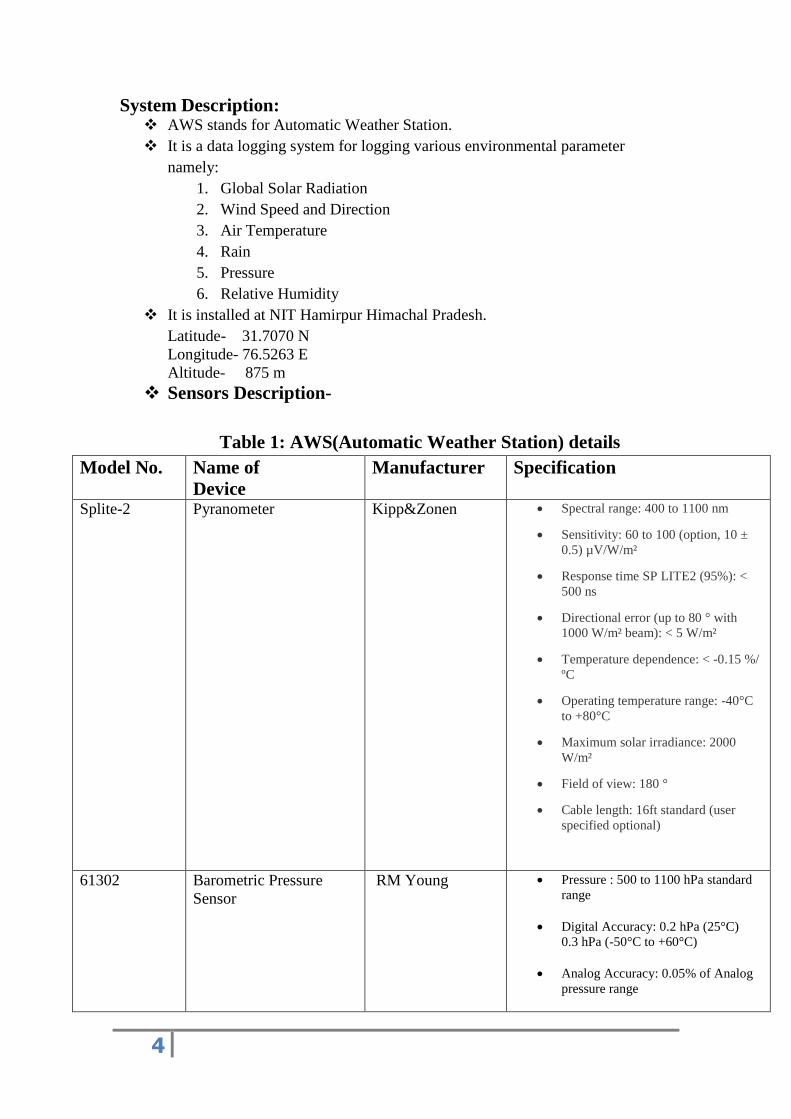
Sensors Description-

Table 1: AWS(Automatic Weather Station) details

Model No. Name of

Device

Manufacturer Specification

Splite-2 Pyranometer Kipp&Zonen Spectral range: 400 to 1100 nm

Sensitivity: 60 to 100 (option, 10 ±

0.5) µV/W/m²

Response time SP LITE2 (95%): <

500 ns

Directional error (up to 80 ° with

1000 W/m² beam): < 5 W/m²

Temperature dependence: < -0.15 %/

ºC

Operating temperature range: -40°C

to +80°C

Maximum solar irradiance: 2000

W/m²

Field of view: 180 °

Cable length: 16ft standard (user

specified optional)

61302 Barometric Pressure

Sensor

RM Young Pressure : 500 to 1100 hPa standard

range

Digital Accuracy: 0.2 hPa (25°C)

0.3 hPa (-50°C to +60°C)

Analog Accuracy: 0.05% of Analog

pressure range

5

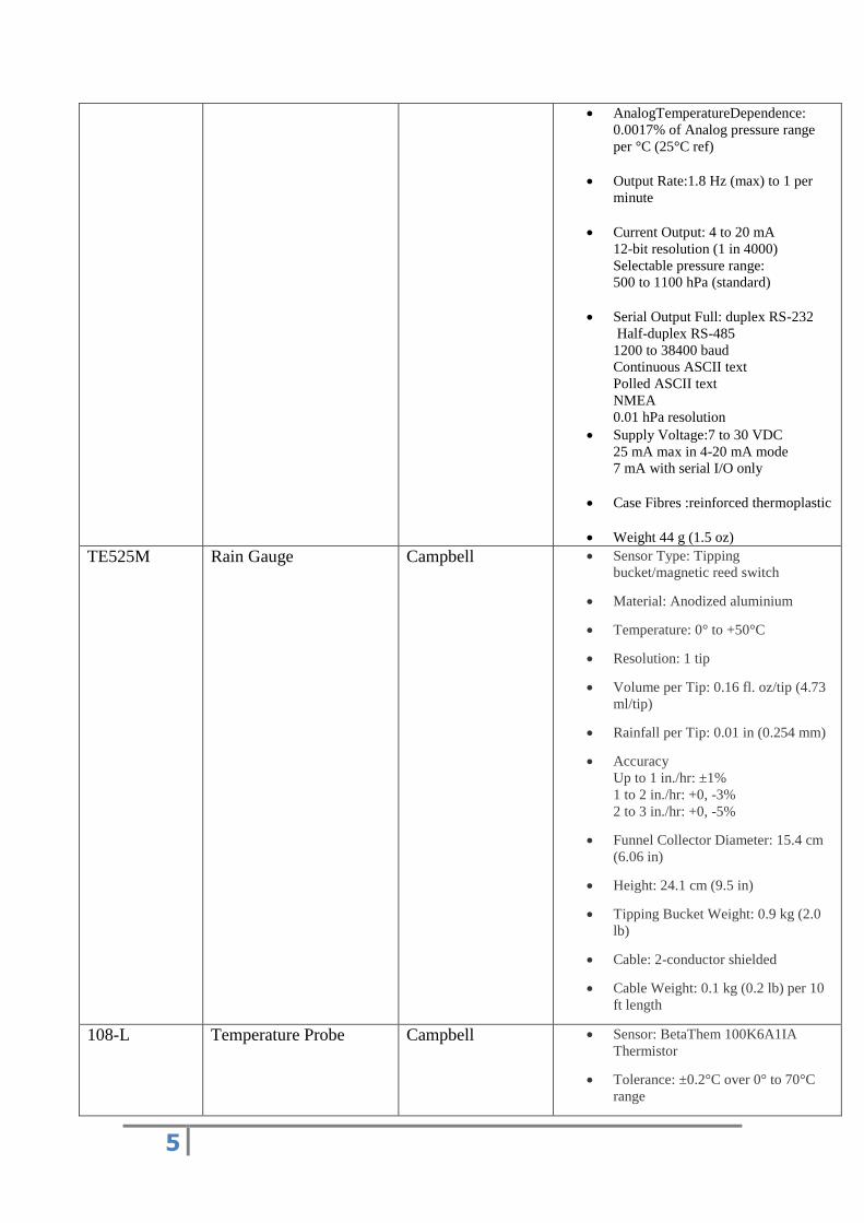
AnalogTemperatureDependence:

0.0017% of Analog pressure range

per °C (25°C ref)

Output Rate:1.8 Hz (max) to 1 per

minute

Current Output: 4 to 20 mA

12-bit resolution (1 in 4000)

Selectable pressure range:

500 to 1100 hPa (standard)

Serial Output Full: duplex RS-232

Half-duplex RS-485

1200 to 38400 baud

Continuous ASCII text

Polled ASCII text

NMEA

0.01 hPa resolution

Supply Voltage:7 to 30 VDC

25 mA max in 4-20 mA mode

7 mA with serial I/O only

Case Fibres :reinforced thermoplastic

Weight 44 g (1.5 oz)

TE525M Rain Gauge Campbell Sensor Type: Tipping

bucket/magnetic reed switch

Material: Anodized aluminium

Temperature: 0° to +50°C

Resolution: 1 tip

Volume per Tip: 0.16 fl. oz/tip (4.73

ml/tip)

Rainfall per Tip: 0.01 in (0.254 mm)

Accuracy

Up to 1 in./hr: ±1%

1 to 2 in./hr: +0, -3%

2 to 3 in./hr: +0, -5%

Funnel Collector Diameter: 15.4 cm

(6.06 in)

Height: 24.1 cm (9.5 in)

Tipping Bucket Weight: 0.9 kg (2.0

lb)

Cable: 2-conductor shielded

Cable Weight: 0.1 kg (0.2 lb) per 10

ft length

108-L Temperature Probe Campbell Sensor: BetaThem 100K6A1IA

Thermistor

Tolerance: ±0.2°C over 0° to 70°C

range

6

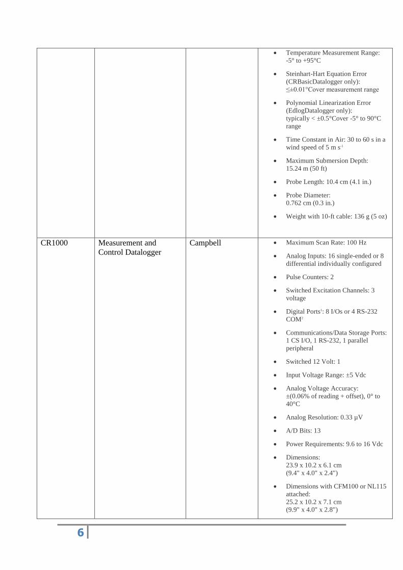
Temperature Measurement Range:

-5° to +95°C

Steinhart-Hart Equation Error

(CRBasicDatalogger only):

≤±0.01°Cover measurement range

Polynomial Linearization Error

(EdlogDatalogger only):

typically < ±0.5°Cover -5° to 90°C

range

Time Constant in Air: 30 to 60 s in a

wind speed of 5 m s-1

Maximum Submersion Depth:

15.24 m (50 ft)

Probe Length: 10.4 cm (4.1 in.)

Probe Diameter:

0.762 cm (0.3 in.)

Weight with 10-ft cable: 136 g (5 oz)

CR1000 Measurement and

Control Datalogger

Campbell Maximum Scan Rate: 100 Hz

Analog Inputs: 16 single-ended or 8

differential individually configured

Pulse Counters: 2

Switched Excitation Channels: 3

voltage

Digital Ports1: 8 I/Os or 4 RS-232

COM2

Communications/Data Storage Ports:

1 CS I/O, 1 RS-232, 1 parallel

peripheral

Switched 12 Volt: 1

Input Voltage Range: ±5 Vdc

Analog Voltage Accuracy:

±(0.06% of reading + offset), 0° to

40°C

Analog Resolution: 0.33 µV

A/D Bits: 13

Power Requirements: 9.6 to 16 Vdc

Dimensions:

23.9 x 10.2 x 6.1 cm

(9.4" x 4.0" x 2.4")

Dimensions with CFM100 or NL115

attached:

25.2 x 10.2 x 7.1 cm

(9.9" x 4.0" x 2.8")

7

Weight: 1.0 kg (2.1 lb)

Protocols Supported: PakBus,

Modbus, DNP3, FTP, HTTP, XML,

POP3, SMTP, Telnet, NTCIP, NTP,

SDI-12, SDM

CE Compliance Standards to which

Conformity is Declared:

IEC61326:2002

Warranty: 3 years

Temperature Range

Standard: -25° to +50°C

Extended: -55° to +85°C

Memory

Operating System: 2 MB flash

Battery-Backed SRAM for CPU

Usage and Final Storage: 4 MB

Flash Disk (CPU) for Program Files:

512 kB

Typical Current Drain @ 12 Vdc

Sleep Mode: < 1mA

Active (w/o RS-232

communication):

1 to 16 mA typical

Active (w/RS-232 communication):

17 to 28 mA typical

05103-10-L Wind Monitor RM Young Operating Temperature: -50° to

+50°C, assuming non-riming

conditions

Overall Height: 37 cm (14.6 in.)

Overall Length: 55 cm (21.7 in.)

Main Housing Diameter: 5 cm (2.0

in.)

Propeller Diameter: 18 cm (7.1 in.)

Mounting Pipe Description:

34 mm (1.34 in.) OD; standard 1.0-

in. IPS schedule 40

Weight: 1.5 kg (3.2 lb)

Wind Speed

8

Range: 0 to 100 m/s (0 to 224 mph)

Accuracy:

±0.3 m/s (0.6 mph) or 1% of reading

Starting Threshold: 1.0 m/s (2.2 mph)

Distance Constant (63% recovery):

2.7 m (8.9 ft)

Output:

ac voltage (three pulses per

revolution);

90 Hz (1800 rpm) = 8.8 m/s (19.7

mph)

Wind Direction

Range:

Mechanical: 0 to 360°

Electrical: 355° (5° open)

Accuracy: ±3°

Starting Threshold at 10°

Displacement:

1.1 m/s (2.4 mph)

Damping Ratio: 0.3

Damped Natural Wavelength:

7.4 m (24.3 ft)

Undamped Natural Wavelength:

7.2 m (23.6 ft)

Output: Analog dc voltage from

potentiometer—resistance 10kohms;

linearity 0.25%; life expectancy 50

million revolutions

Power switched excitation voltage

supplied by Datalogger.

HC-S3 Relative Humidity and

Temperature Probe

Rotronic

Instrument Corp.

Relative Humidity Operating range: 0

to 100%

RH Accuracy at 23°C: ±1.5%

RH Output: 0 - 1 VDC

Typical Long-Term Stability: Better

than ±1% RH per year

Temperature Measurement Range: -

40° to +60°C or -50° to +50°C

(model HC-S3-XT)

Temperature Accuracy: -30°C -

+60°C: ±0.2°C or -50°C - +60°C:

±0.6°C (worst case)

9

Output: 0 - 1 VDC

General Supply Voltage: 3.5 to 50

VDC (typically powered by data

logger’s 12 VDC supply)

Current Consumption: < 4 mA

Diameter: 0.6” (15.25 mm)

Length: 6.6” (168 mm)

Methodology

Method of Bins

First Separate data into wind speed intervals or bins.

Let there are NB no of bins with bin width Wj , mjmean speed in bin duration,

with fi no of occurrences or frequency in each bin

Then

Total Occurrence:

Average Wind Speed:

Standard deviation:

Average Wind Power:

10

Analysis By Using WAsP

‘AWS 1min-2013’ Observed Wind Climate

Produced on 09-02-2015 at 15:02:35 by using WAsP version: 11.02.0062.

Site description: 'CEEE Nit Hamirpur'; Position: 31.63°N 76.51°E; Anemometer

height: 18.5 m from roof top of centre.

Table2: Mean wind speed and power density using WAsP

Parameter Measure

d

Emergen

t

Discrepanc

y

Mean wind speed [m/s] unknown 1.89 unknown

Mean power density

[W/m²]

unknown 9 W/m² unknown

Fig 1: Wind Rose Fig 2: Weibull PDF curve

Table3: Using WAsP Weibull distribution parameter

0 30 60 90 120 150 180 210 240 270 300 330

A 2.3 2.3 2.2 1.8 1.7 1.8 2.0 1.8 1.7 1.9 2.4 2.6

k 1.94 1.97 1.64 1.28 1.21 1.64 2.23 1.70 1.40 1.49 1.97 2.29

U 2.06 2.05 1.95 1.67 1.60 1.62 1.80 1.58 1.57 1.70 2.17 2.34

P 10 10 11 10 10 6 6 6 7 8 12 13

f 9.6 9.8 10.4 6.9 6.0 9.2 13.1 6.2 4.9 4.6 8.0 11.3

Table 4: Wind Rose data table

U 0 30 60 90 120 150 180 210 240 270 300 330 All

1.0 215 209 213 329 374 286 201 348 399 369 224 162 255

2.0 312 320 372 405 388 453 415 365 323 294 268 249 349

3.0 307 319 287 161 129 203 323 219 185 213 299 352 266

4.0 119 110 81 53 52 33 52 53 67 86 153 178 90

5.0 33 29 26 26 29 13 7 11 17 27 41 43 25

6.0 9 9 11 13 16 7 2 2 5 8 10 11 8

7.0 2 3 5 7 7 3 1 1 1 2 3 3 3

8.0 1 1 3 4 3 1 0 1 1 1 1 1 1

9.0 0 0 1 2 1 1 0 0 0 1 1 0 1

11

10. 0 0 1 1 0 0 0 0 0 0 0 0 0

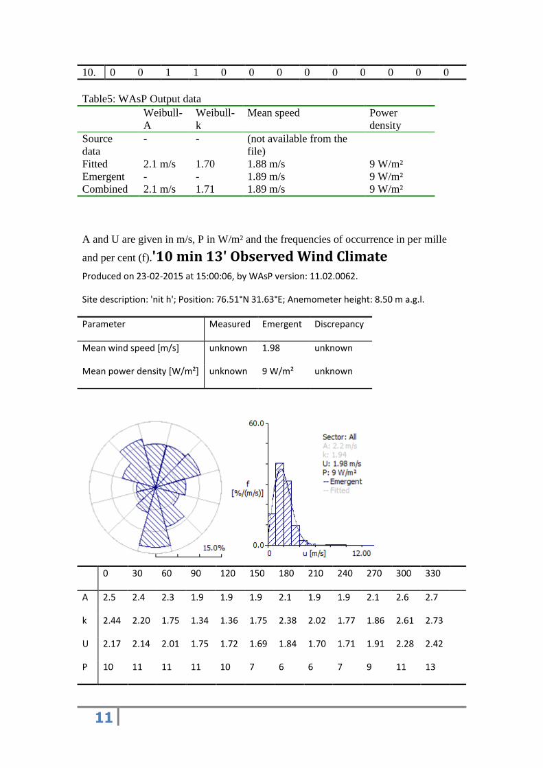
Table5: WAsP Output data

Weibull-

A

Weibull-

k

Mean speed Power

density

Source

data

- - (not available from the

file)

Fitted 2.1 m/s 1.70 1.88 m/s 9 W/m²

Emergent - - 1.89 m/s 9 W/m²

Combined 2.1 m/s 1.71 1.89 m/s 9 W/m²

A and U are given in m/s, P in W/m² and the frequencies of occurrence in per mille

and per cent (f).'10 min 13' Observed Wind Climate Produced on 23-02-2015 at 15:00:06, by WAsP version: 11.02.0062.

Site description: 'nit h'; Position: 76.51°N 31.63°E; Anemometer height: 8.50 m a.g.l.

Parameter Measured Emergent Discrepancy


Mean power density [W/m²] unknown 9 W/m² unknown

0 30 60 90 120 150 180 210 240 270 300 330

A 2.5 2.4 2.3 1.9 1.9 1.9 2.1 1.9 1.9 2.1 2.6 2.7

k 2.44 2.20 1.75 1.34 1.36 1.75 2.38 2.02 1.77 1.86 2.61 2.73

U 2.17 2.14 2.01 1.75 1.72 1.69 1.84 1.70 1.71 1.91 2.28 2.42

P 10 11 11 11 10 7 6 6 7 9 11 13

12

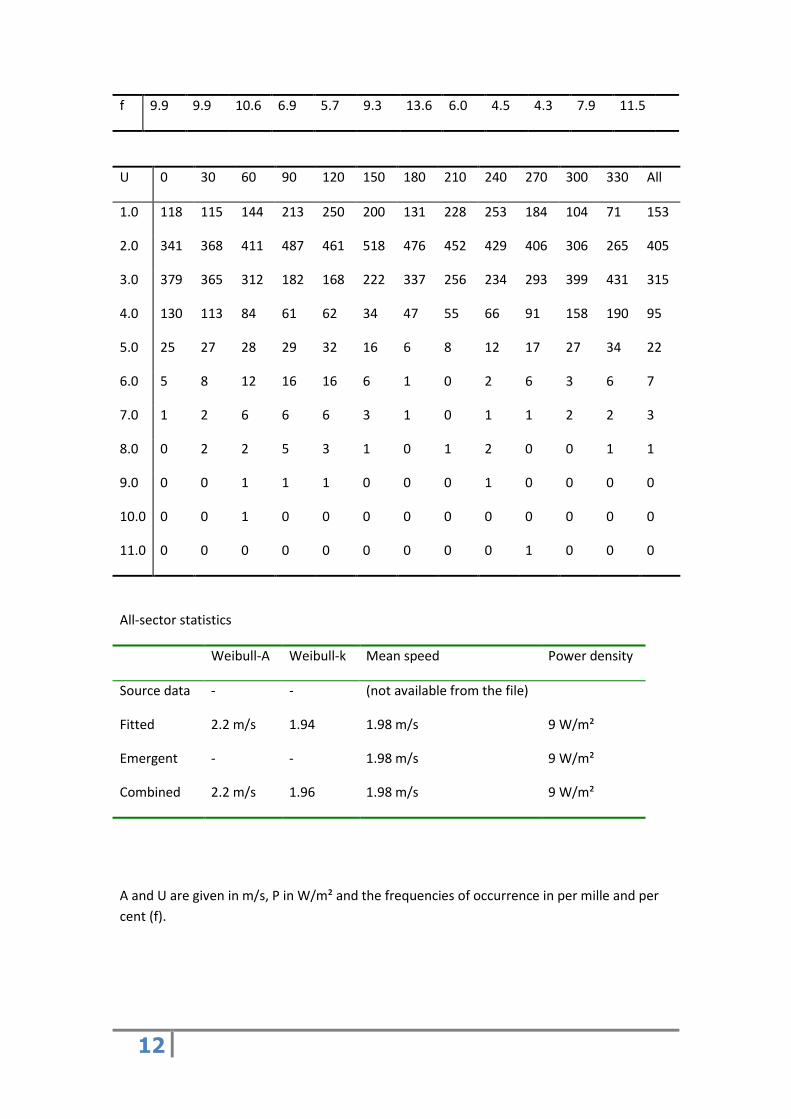
f 9.9 9.9 10.6 6.9 5.7 9.3 13.6 6.0 4.5 4.3 7.9 11.5

U 0 30 60 90 120 150 180 210 240 270 300 330 All

1.0 118 115 144 213 250 200 131 228 253 184 104 71 153

2.0 341 368 411 487 461 518 476 452 429 406 306 265 405

3.0 379 365 312 182 168 222 337 256 234 293 399 431 315

4.0 130 113 84 61 62 34 47 55 66 91 158 190 95

5.0 25 27 28 29 32 16 6 8 12 17 27 34 22

6.0 5 8 12 16 16 6 1 0 2 6 3 6 7

7.0 1 2 6 6 6 3 1 0 1 1 2 2 3

8.0 0 2 2 5 3 1 0 1 2 0 0 1 1

9.0 0 0 1 1 1 0 0 0 1 0 0 0 0

10.0 0 0 1 0 0 0 0 0 0 0 0 0 0

11.0 0 0 0 0 0 0 0 0 0 1 0 0 0

All-sector statistics

Weibull-A Weibull-k Mean speed Power density

Source data - - (not available from the file)

Fitted 2.2 m/s 1.94 1.98 m/s 9 W/m²


Combined 2.2 m/s 1.96 1.98 m/s 9 W/m²

A and U are given in m/s, P in W/m² and the frequencies of occurrence in per mille and per

cent (f).

13

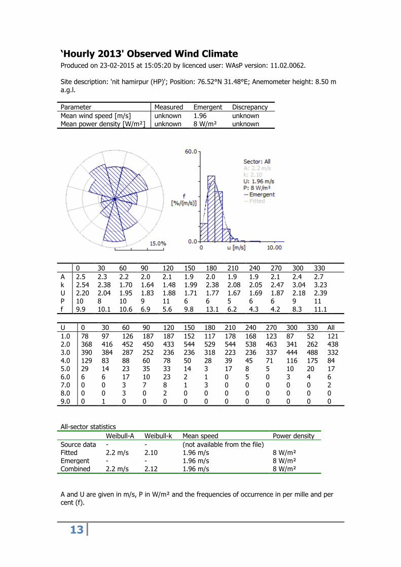
‘Hourly 2013' Observed Wind Climate Produced on 23-02-2015 at 15:05:20 by licenced user: WAsP version: 11.02.0062.

Site description: 'nit hamirpur (HP)'; Position: 76.52°N 31.48°E; Anemometer height: 8.50 m

a.g.l.




0 30 60 90 120 150 180 210 240 270 300 330

A 2.5 2.3 2.2 2.0 2.1 1.9 2.0 1.9 1.9 2.1 2.4 2.7 k 2.54 2.38 1.70 1.64 1.48 1.99 2.38 2.08 2.05 2.47 3.04 3.23

U 2.20 2.04 1.95 1.83 1.88 1.71 1.77 1.67 1.69 1.87 2.18 2.39 P 10 8 10 9 11 6 6 5 6 6 9 11

f 9.9 10.1 10.6 6.9 5.6 9.8 13.1 6.2 4.3 4.2 8.3 11.1

U 0 30 60 90 120 150 180 210 240 270 300 330 All

1.0 78 97 126 187 187 152 117 178 168 123 87 52 121 2.0 368 416 452 450 433 544 529 544 538 463 341 262 438

3.0 390 384 287 252 236 236 318 223 236 337 444 488 332

4.0 129 83 88 60 78 50 28 39 45 71 116 175 84 5.0 29 14 23 35 33 14 3 17 8 5 10 20 17

6.0 6 6 17 10 23 2 1 0 5 0 3 4 6 7.0 0 0 3 7 8 1 3 0 0 0 0 0 2

8.0 0 0 3 0 2 0 0 0 0 0 0 0 0

9.0 0 1 0 0 0 0 0 0 0 0 0 0 0



Source data - - (not available from the file) Fitted 2.2 m/s 2.10 1.96 m/s 8 W/m²

Emergent - - 1.96 m/s 8 W/m² Combined 2.2 m/s 2.12 1.96 m/s 8 W/m²

A and U are given in m/s, P in W/m² and the frequencies of occurrence in per mille and per cent (f).

14

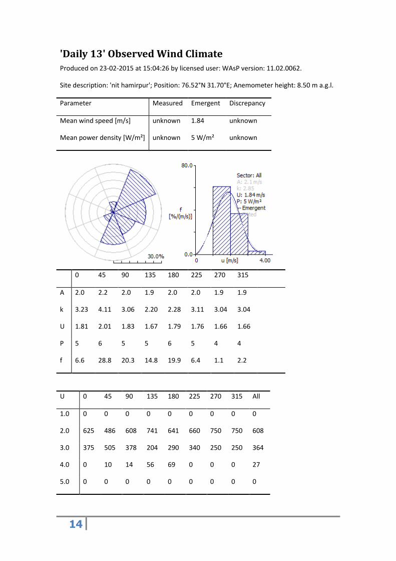
'Daily 13' Observed Wind Climate Produced on 23-02-2015 at 15:04:26 by licensed user: WAsP version: 11.02.0062.

Site description: 'nit hamirpur'; Position: 76.52°N 31.70°E; Anemometer height: 8.50 m a.g.l.




0 45 90 135 180 225 270 315

A 2.0 2.2 2.0 1.9 2.0 2.0 1.9 1.9

k 3.23 4.11 3.06 2.20 2.28 3.11 3.04 3.04

U 1.81 2.01 1.83 1.67 1.79 1.76 1.66 1.66

P 5 6 5 5 6 5 4 4

f 6.6 28.8 20.3 14.8 19.9 6.4 1.1 2.2

U 0 45 90 135 180 225 270 315 All

1.0 0 0 0 0 0 0 0 0 0

2.0 625 486 608 741 641 660 750 750 608

3.0 375 505 378 204 290 340 250 250 364

4.0 0 10 14 56 69 0 0 0 27

5.0 0 0 0 0 0 0 0 0 0

15



Source data - - (not available from the file)

Fitted 2.1 m/s 2.85 1.83 m/s 5 W/m²


Combined 2.1 m/s 2.88 1.84 m/s 5 W/m²

A and U are given in m/s, P in W/m² and the frequencies of occurrence in per mille and per cent (f).

Analysis by using ‘Method of Bins’

Table6: Yearly Average Comparison table

Parameters AWS Data 2013 NASA Data

2013

1 min 10 Min Hourly Daily Daily

Average

Wind Speed

(U) (m/s)

1.9639 1.9648 1.9641 1.9663 2.3801

Standard

Deviation

1.0651 0.9671 0.8524 0.3744 0.5518

Average

Wind Power

Density (P/A)

9.7384 8.7357 7.7235 5.2120 9.7641

Table7: Season wise analysis

Parameters

10 Minute data 2013

Winter Summer Rainy Spring

Average Wind

Speed (U)

(m/s)

2.0056 2.2280 1.6884 1.7464

Standard

Deviation

0.9782 0.9576 0.9764 0.9673

Average Wind

Power Density

(P/A)

8.4592 8.9843 8.1532 8.2983

16

Table8: Season Classification

Season Months

Winter Jan, Feb, March, November, December.

Summer April, May June

Rainy July, August

Spring September, October

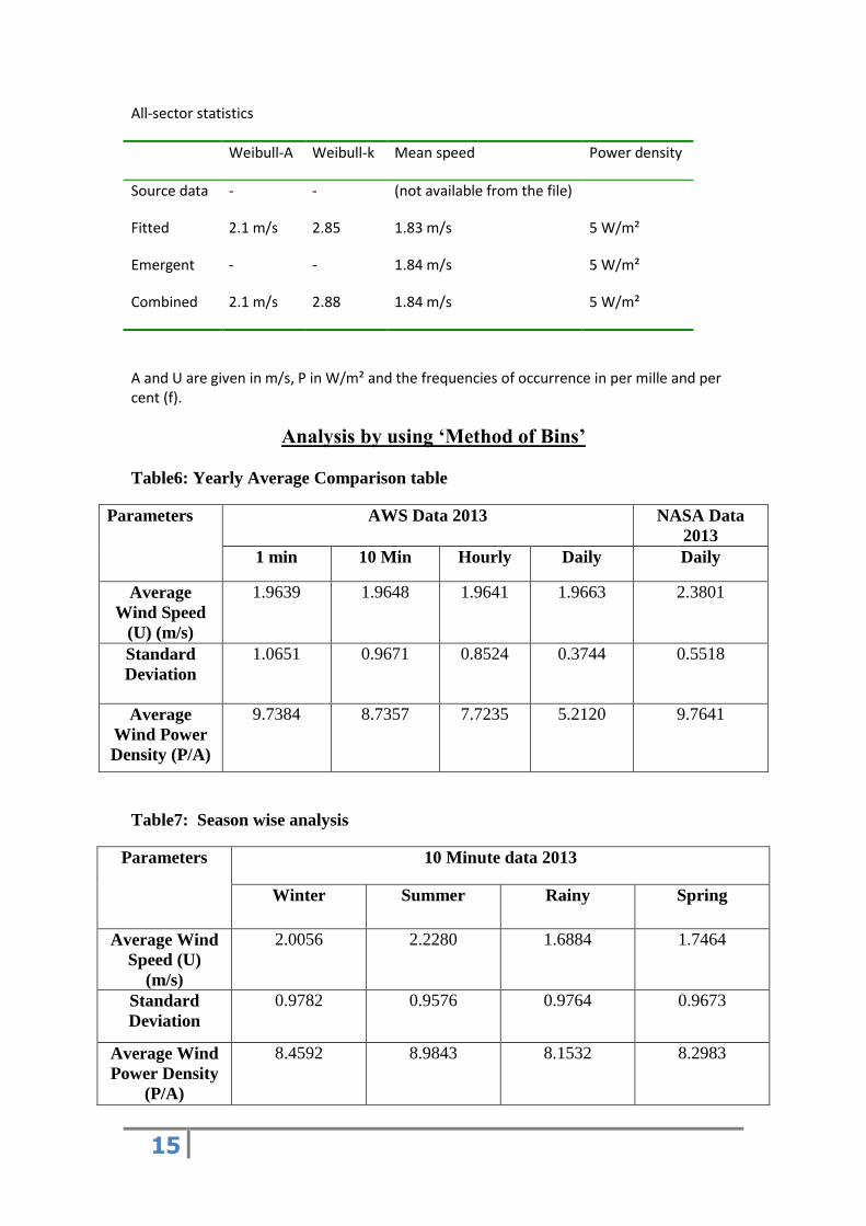
Figure3:Manual Histogram 1-min Data

17

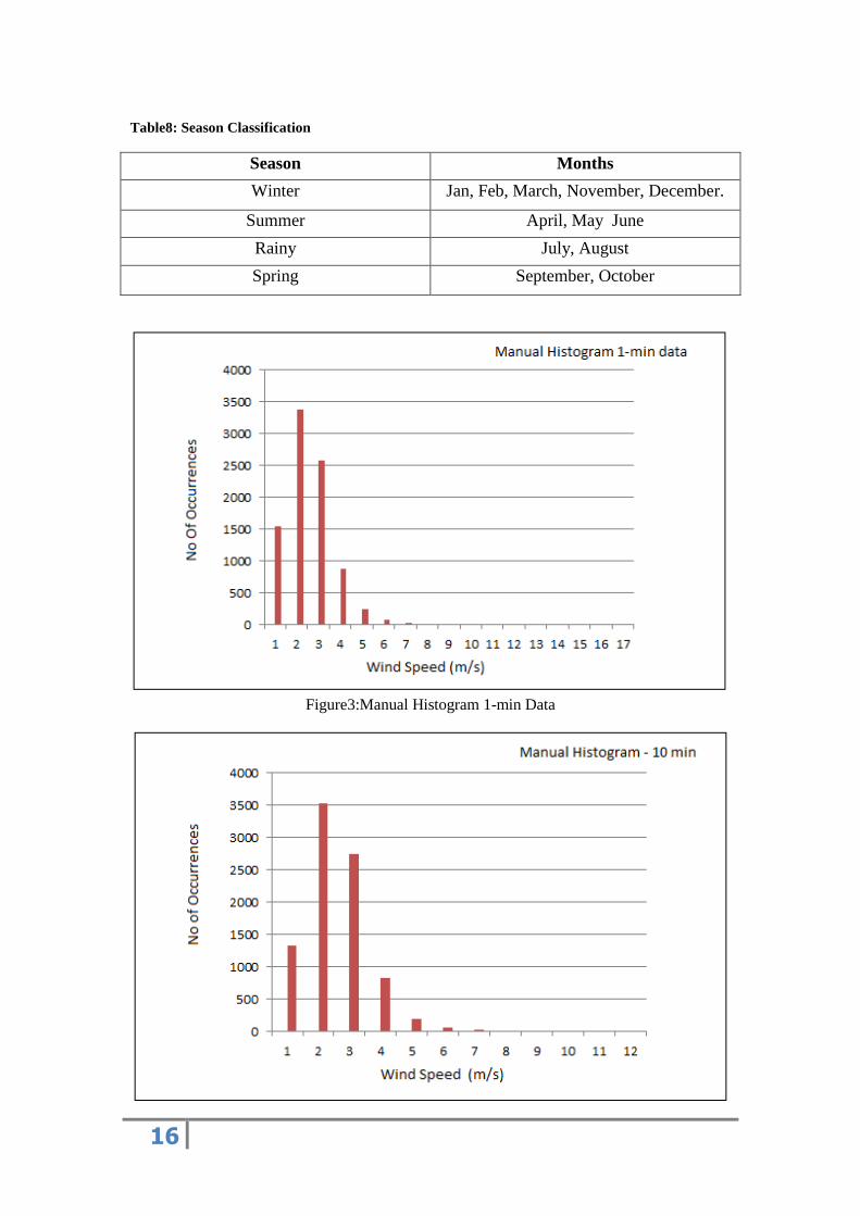
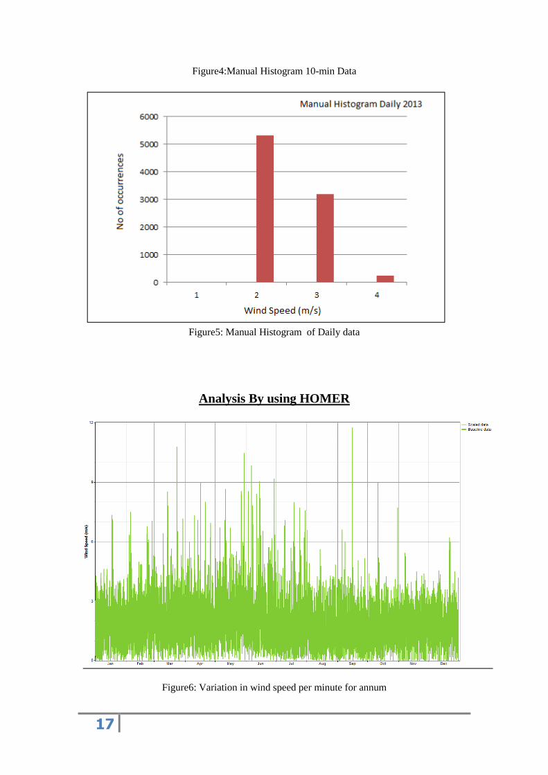
Figure4:Manual Histogram 10-min Data

Figure5: Manual Histogram of Daily data

Analysis By using HOMER

Figure6: Variation in wind speed per minute for annum

18

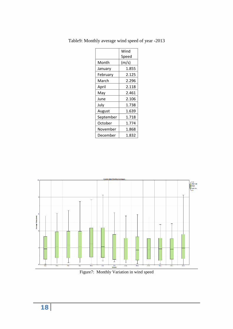
Table9: Monthly average wind speed of year -2013

Wind Speed

Month (m/s)

January 1.855

February 2.125

March 2.296

April 2.118

May 2.461

June 2.106

July 1.738

August 1.639

September 1.718

October 1.774

November 1.868

December 1.832

Figure7: Monthly Variation in wind speed

19

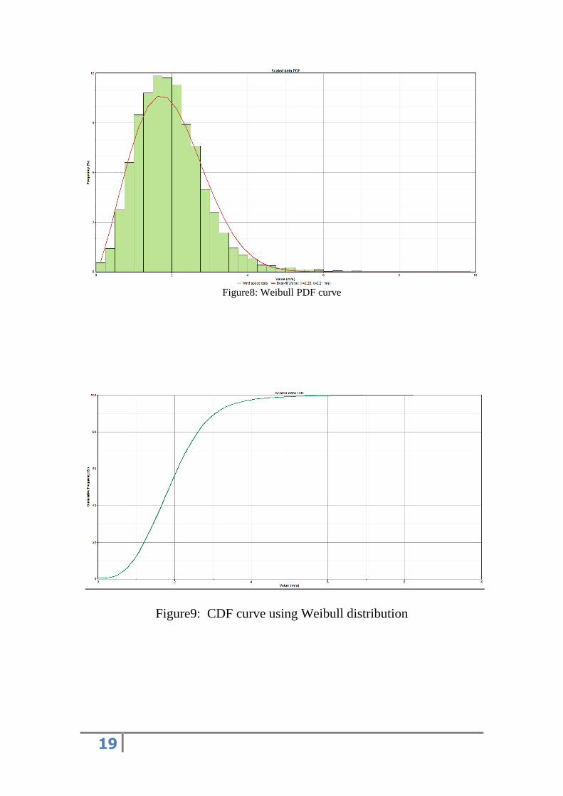
Figure8: Weibull PDF curve

Figure9: CDF curve using Weibull distribution

20

Results and Analysis:

From the monthly average wind speed (Refer table no. 9 ) we can see that-

o Maximum average wind speed is in the month of May, in the

summer season.

o Minimum average wind speed is in the month of August, the rainy

season.

From the Bins method (Refer table no. 6 ) we can see that-

o Maximum occurrence of wind speed is between the range of

2-3 m/s throughout a year-2013

o This range varies based on observation frequency. For example

o If we are taking wind data in 1 minute interval, the range is

1- 2 m/s.(see figure 3)

o If the wind data interval is 10 minute then this range is

2-3 m/s.(See figure 4)

o If the wind data interval is hourly average data then this

range is also 2-3 m/s with more occurrences.(See figure 5)

From HOMER analysis of 2013 year wind data we can see that:

o The wind speed variation minute wise for full year in figure 6.

o The monthly variation of wind speed for year 2013 in figure 7.

o Weibull distribution curve using Homer is shown in figure 8.

Documents

A Report On Wind Data from Automatic Weather Station (AWS) of 2013 at Nit Hamirpur