A regional-scale particle-tracking method for nonstationary fractured media

$Page 1: A regional-scale particle-tracking method for nonstationary fractured media$
A regional-scale particle-tracking method for nonstationary

fractured media

Johan Ohman and Auli Niemi

Air and Water Science, Department of Earth Sciences, Uppsala University, Uppsala, Sweden

Chin-Fu Tsang

Earth Sciences Division, Lawrence Berkeley National Laboratory, Berkeley, California, USA

Received 16 July 2004; revised 13 December 2004; accepted 17 January 2005; published 18 March 2005.

[1] A regional-scale transport model is introduced that is applicable to nonstationary andstatistically inhomogeneous fractured media, provided that hydraulic flow, but notnecessarily solute transport, can be approximated by equivalent continuum properties atsome block scale. Upscaled flow and transport block properties are transferred frommultiple fracture network realizations to a regional model with grid elements of size equalto that found valid for continuum approximation of flow. In the regional-scale model,flow is solved in a stochastic continuum framework, whereas the transport calculationsemploy a random walk procedure. Block-wise transit times are sampled from distributionslinked to each block based on its underlying fracture network. To account for channeledtransport larger than the block scale, several alternative sampling algorithms areintroduced and compared. The most reasonable alternative incorporates a spatialpersistence length in sampling the particle transit times; this tracer transport persistencelength is related to interblock channeling, and is quantified by the number N of blocks.The approach is demonstrated for a set of field data, and the obtained regional-scaleparticle breakthroughs are analyzed. These are fitted to the one-dimensional advective-dispersive equation to determine an effective macroscale dispersion coefficient for theregional scale. An interesting finding is that this macroscale dispersion coefficient is foundto be a linear function of the transport persistence, N, with a slope equal to a representativemean block-scale dispersion coefficient and a constant that incorporates backgrounddispersion arising from the regional heterogeneous conductivity field.

Citation: Ohman, J., A. Niemi, and C.-F. Tsang (2005), A regional-scale particle-tracking method for nonstationary fractured media,

Water Resour. Res., 41, W03016, doi:10.1029/2004WR003498.

1. Introduction

[2] Modeling flow and transport in fractured rock iscomplicated by strong heterogeneity. This makes predic-tions of tracer transport from local observations and theirupscaling for large-scale models a challenging task. Never-theless, it is often necessary to use small-scale data asregional-scale data for fractured rock are rare, owing tothe slow responses of hydraulic cross-hole tests and tracertransport experiments.[3] Tsang and Neretnieks [1998] reviewed available field

experiments and analysis methods. More recently, tracerexperiments for transport characterization in fracturedmedia have been carried out at small scale [e.g., Sidle etal., 1998], intermediate scale [Kosakowski, 2004], andkilometer scale [Becker and Shapiro, 2000; Shapiro,2001]. As pointed out by Tsang and Neretnieks [1998]the tracer breakthrough curves typically display anomalousbreakthrough curves that are characterized by early initialarrival and extraordinarily long tails exhibiting slow decay.The impossibility of fitting the analytical one-dimensional

advection-dispersion equation (ADE) to the breakthroughcurves indicates that this tailing may result from variableadvective velocity among different flow paths (Kosakowski[2004]; Becker and Shapiro [2000]; Shapiro [2001]; seealso Tsang and Tsang [1987] and Moreno and Tsang[1994]) and/or diffusive mass transfer between flow pathsand either stagnant water or an essentially infinite rockmatrix [Cvetkovic et al., 1999; Andersson et al., 2004].[4] In terms of modeling, three basic approaches are

commonly adopted: (1) the deterministic equivalent porousmedium approach, (2) the stochastic continuum approach,and (3) the fracture network approach. The range ofapplicability of these alternative approaches depends onthe scale of the heterogeneity in relation to the scale ofthe region of interest. The deterministic-porous mediumapproach is applicable to the largest of scales, and thefracture network approach is applicable to the smallest ofscales where flow and transport in individual fractures maybe important. The applicability range of the stochasticcontinuum approach falls in between these cases, i.e., atscales where the heterogeneity effects are of interest but canbe represented by stochastic continuum properties. A moredetailed review of different approaches to modeling flow infractured media is given by Ohman and Niemi [2003].

Copyright 2005 by the American Geophysical Union.0043-1397/05/2004WR003498

W03016

WATER RESOURCES RESEARCH, VOL. 41, W03016, doi:10.1029/2004WR003498, 2005

1 of 16

Several recent works also employ some hybrid approachwhere fracture network models are used to derive input forstochastic continuum models. In such cases, the scale atwhich the continuum approximation can be adopted must beproperly determined [Long et al., 1982; Cacas et al., 1990a;National Research Council (NRC), 1996].[5] A variety of experiments have demonstrated [e.g.,

Neretnieks, 1993] that the distribution of transport pathwaysin fractured rocks can be very different from observed flowpatterns. Therefore transport does not necessarily exhibitcontinuum behavior at the same support scale for whichcontinuum conductivity tensors can be determined for flow[Endo et al., 1984; Cacas et al., 1990b; Abelin et al., 1991].Furthermore, even if an effective transport property can bedetermined at some meaningful support scale to justify theuse of a stochastic continuum analysis for transport, thefinite difference and finite element solutions of the ADE instrongly heterogeneous conductivity fields can show severenumerical dispersion [e.g., Hoffman, 2001].[6] Because of the difficulties in applying continuum

models for transport, on the one hand, and the limits ofapplicability of fracture network models on the other, newinnovative methods are needed to solve regional-scaleproblems [NRC, 1996; Berkowitz, 2002]. Many of the recentapproaches rely on various forms of stochastic Lagrangianmethods [e.g., Xu et al., 2001; Bruderer and Bernabe, 2001;Cvetkovic et al., 2004]. Typically, they use a combination ofparticle tracking and random walk [e.g., Scher et al., 2002].In their pioneering work, Schwartz and Smith [1988]introduced a hybrid method to upscale fracture network-based transport to be used as input for a large-scaleequivalent-porous-medium model, and owing to its feasi-bility, their approach is still in use [e.g., Abbo et al., 2003;Carneiro, 2003]. In this approach, stochastic particle motionis learned from particle tracking in a ‘‘subdomain’’ fracturenetwork which is exposed to a gradually rotated hydraulicgradient. Assuming statistical homogeneity, fitted particle-motion distributions are then sampled in a random walkthrough a regional-scale head field, which is solved bydeterministic continuum modeling. This approach was laterimproved by accounting for preferential flow [Parney andSmith, 1995], by including correlation between particlevelocity and path length that is also determined from the‘‘subdomain.’’ Recently, the linear Boltzmann transportequation was used in a rather similar hybrid approach todescribe particle motion in fractured media [Benke andPainter, 2003]. Fracture intersections are represented by‘‘molecule collisions’’ in a fluid, in the sense that they maycause abrupt changes in the direction and velocity of aparticle during a random walk. Preferential flow isaccounted for by fracture-intersection-transition probabili-ties which are obtained from particle tracking in smallfracture networks.[7] In spite of the great progress made during the last

20 years in characterizing and describing flow and transportin fractured media, models for field-scale transport are stillpreliminary in character in terms of their capability to takesite-specific heterogeneity into account. The present workintroduces a new approach to this problem. We start fromthe detailed-scale geological and hydraulic data and employfracture network modeling to obtain the relevant flow andtransport statistics at some support scale, for which flow,

but not necessarily transport, can be represented by meansof a continuum. We then use stochastic continuum flowsimulation in combination with particle tracking to modellarge-scale transport. Here particle velocities determinedfrom the network realizations are transferred to a large-scale model via a specific scaling method. Special attentionis given to transport channeling characteristics; this ismodeled by a superimposed ‘‘tracer transport persistence,’’N, in our sampling algorithm. Furthermore, to demonstratethe feasibility of allowing for realistic field conditions thatoften exhibit nonstationarity, we include a depth trend inflow and transport characteristics caused by the closing offractures with increasing stress. To keep the focus on thetheoretical development of upscaling of flow and transportfrom local fracture networks to the regional model, we donot include matrix diffusion in the present model. Exten-sions to account for this would be rather straightforward toimplement in the particle-tracking scheme embedded in ourmethod. Delayed breakthrough times that account formatrix diffusion and linear sorption could be calculatedusing methods by Tsang and Tsang [2001] and Tsang andDoughty [2003] and be transferred into the regional-scalemodel using our scheme.[8] In the following, we will first present our approach,

and then apply it to a set of field data to study a hypotheticalscenario related to deep disposal of high-level nuclearwaste. We use data from Sellafield, England, as an example[Andersson and Knight, 2000]. Sellafield is a fractured rocksite that has been intensively investigated by Nirex [e.g.,Nirex, 1997a, 1997b, 1997c, 1997d] in connection withnuclear waste disposal. The database we use is not completeand is not intended to reflect the characteristics of the site ingeneral, but is taken merely as an example of a realisticfractured rock database to demonstrate our method.

2. Model for Regional-Scale Transport inFractured Media

2.1. Overview of the Model

[9] Our objective is to introduce a model for regional-scale solute transport in fracture media that properly honorsthe fracture-related heterogeneity observed in boreholes viaa fracture network-based upscaling. The approach adoptedis inspired by Nordqvist et al. [1992], who transferredstatistics of within-fracture plane channeled transportevoked by variable aperture, onto a flow field solved for aconstant-aperture fracture network. In their approach, transittime distributions are first determined by particle tracking inindividual fracture planes with variable aperture. Transportis then modeled by a random walk through a three-dimen-sional fracture network [Dverstorp and Andersson, 1989],where at each fracture, the previously obtained distributionsare sampled with appropriate rescaling for local gradients[Tsang, 1993]. In this paper we seek to utilize theirinnovative concept, but at a larger scale, as explained below.[10] The three different scales being addressed here are

regional scale, block scale, and detailed scale. We define theregional scale by a kilometer-scale domain for whichtransport is ultimately to be solved. The block scale isdefined by a cubic domain, for which fracture network flowcan be represented by conductivity tensors of equivalentporous media (i.e., it is the scale for valid ‘‘continuum

2 of 16

W03016 OHMAN ET AL.: REGIONAL-SCALE TRANSPORT IN FRACTURED MEDIA W03016

approximation’’ of hydraulic flow). For the current data set,an earlier study [Ohman and Niemi, 2003] found the blockscale to have side length 7.5 m. The detailed scale refers tofracture network geometry and individual fractures thatgovern the transport properties of the medium (and inparticular of the blocks). Our approach relies on a ‘‘hybrid’’concept where the detailed fracture-scale properties aretransferred via the block scale to the regional scale. It canbriefly be summarized as follows:[11] 1. The hydraulic characteristics of a large number

of fracture network realizations are studied to determinecontinuum tensors for hydraulic conductivity at the blockscale, which is then used as a support scale [Neuman,1987] in a regional-scale stochastic continuum model.[12] 2. Tracer-transport behavior is learned from the same

block-scale fracture networks as were used to determine thecontinuum conductivity tensors. A large number of particlesare released within the fracture network blocks, and thedistributions of particle transit times are measured andcollected in probability distributions. It can be expected(as demonstrated later) that transport does not exhibitcontinuum characteristics at the block scale, and hence anequivalent dispersion tensor approach cannot be used.Consequently, distributions of particle transit times at blockscale will be used directly in the subsequent regional-scalesimulations.[13] 3. Regional-scale flow fields are simulated with a

stochastic continuum model. This model is discretized to theblock scale, and the distribution of upscaled conductivity,determined in step 1, is used as input.[14] 4. Regional-scale transport is modeled in terms of

particle steps by sampling from the previously obtainedblock-scale transit times. Each upscaled block conductivityvalue is linked to its own transit time distribution, sincesteps 1 and 2 are conducted for the same network realiza-tions, representing the same block. Special emphasis isgiven to how this sampling is done, as will be discussedin more detail later. Furthermore, to obtain the proper transittime at each step in the regional-scale model, the sampledtransit times need to be scaled according to the localambient hydraulic gradient.[15] Step 1 uses fracture network modeling to provide

block conductivities for the regional-scale model (rather thanusing hydraulic data directly). This allows (1) the continuumapproximation for flow to be shown as indeed valid for thesupport scale used, (2) an estimate of anisotropy effects, and(3) the systematic linkage between flow and transportbehaviors of individual fracture network realizations.[16] It should be pointed out that the suggested approach

is highly dependent on the possibility of creating equivalentcontinuum representation of flow for the medium at someblock scale. This is not always attainable, for example, incases where a medium displays certain types of multiscaleor fractal heterogeneity [e.g., Odling, 1997; Le Borgne etal., 2004]. It has been shown that multiscale heterogeneityis to be expected for fracture networks that exhibit particularfractal relationships in the spatial distribution of fractures[Bour and Davy, 1999; Darcel et al., 2003], their fracturelength distribution [Odling, 1997; Bour and Davy, 1998],and/or in aperture correlation to fracture lengths [de Dreuzyet al., 2002]. How our method should be extended for suchdata is a topic for a separate study. It should be noted,

however, that some approaches for fractal-scaled media doemploy continuum approximation at some support scale[e.g., Liu et al., 2004].[17] The software used for the fracture network modeling

are FracMan [Dershowitz et al., 1998], to generate thecomplex three-dimensional fracture network geometries,and MAFIC [Miller et al., 1999], to solve the flow equa-tions and particle transport within these networks. At theregional scale, the GSLIB software [Deutsch and Journel,1998] is used to generate correlated stochastic conductivityfields, and TOUGH [Pruess et al., 1999], an integral finitedifference-based code, is used to solve the flow fields. Theregional-scale transport was modeled by a particle randomwalk code developed to demonstrate the present transportanalysis. The following sections describe the various stepsin more detail.

2.2. Upscaling Fracture Network Properties atBlock Scale

2.2.1. Block-Scale Hydraulic Conductivity[18] For upscaling hydraulic conductivities, we use the

classical upscaling of fractured media introduced by Long etal. [1982], and later implemented by, for example, Cacas etal. [1990a]. This analysis was carried out for the presentdata as described by Ohman and Niemi [2003]; hence onlythe main points will be repeated here. In this approach, animposed hydraulic gradient is gradually rotated with respectto the fracture network to determine the equivalent conduc-tivity K in each direction. If the shape of this conductivity(as 1/

p(K)) versus rotational angle resembles a smooth

ellipse, its conductivity can be represented by means of acontinuum conductivity tensor. The earlier study foundmost of the fracture network realizations to be sufficientlywell represented by a continuum with a block size of 7.5 m.One reason is that the medium studied here is characterizedby high fracture density, impervious matrix, and low,lognormally distributed fracture transmissivity [Nirex,1997a, 1997b, 1997c, 1997d; Ohman and Niemi, 2003].Note that, in general, the size (and even the existence) ofthis block for continuum approximation depends entirely onthe properties of the fracture network.[19] Flow is simulated at this block scale for multiple

stochastic realizations, i, to determine distributions of con-tinuum conductivity tensors. Only the horizontal and verti-cal components of conductivity are used below as input forgenerating stochastic continuum realizations for the two-dimensional finite difference–based regional-scale model.[20] The hydraulic conductivity of fractured rock is often

found to decrease with increasing depth, due to fracturesclosing with increasing stress. Such a depth trend is incor-porated into the model, based on a hydromechanicalcoupling described in detail by Ohman et al. [2005]. Inprinciple, this approach accounts for fracture closure byusing laboratory data on stress-induced aperture closure. Inthe present work, the rock is divided into four differentdepth intervals j for which the principal stresses are known.Separate statistical distributions of conductivity are thenobtained from fracture networks subject to fracture closureinduced by the stress regime at each depth interval j.2.2.2. Block-Scale Transport Properties[21] Particle transport is then studied at the block scale at

which the continuum representation of flow is found valid.

W03016 OHMAN ET AL.: REGIONAL-SCALE TRANSPORT IN FRACTURED MEDIA

3 of 16

W03016

It would have been convenient, if equivalent continuumdispersivity could be found in a similar way and at the samescale. This is studied by analyzing particle breakthrough asa function of rotational angle. The criteria set for validcontinuum approximation of transport are (1) particlebreakthrough must follow the analytical solution of theadvective-dispersive equation (ADE) and (2) its deriveddispersivity must, as a function of rotational angle, follow atensorial transformation. As will be shown later, the resultsindicate that a dispersion tensor representation is not valid atthe block scale studied. We therefore use another approachto transfer block-scale particle transit times, t, to theregional-scale stochastic continuum model. The transit timeis defined as

t sð Þ ¼Zs0

ds

v sð Þ ; ð1Þ

where v is the spatially varying fluid velocity along thetrajectory at a distance s from the release point.[22] To obtain particle transit times for each fracture

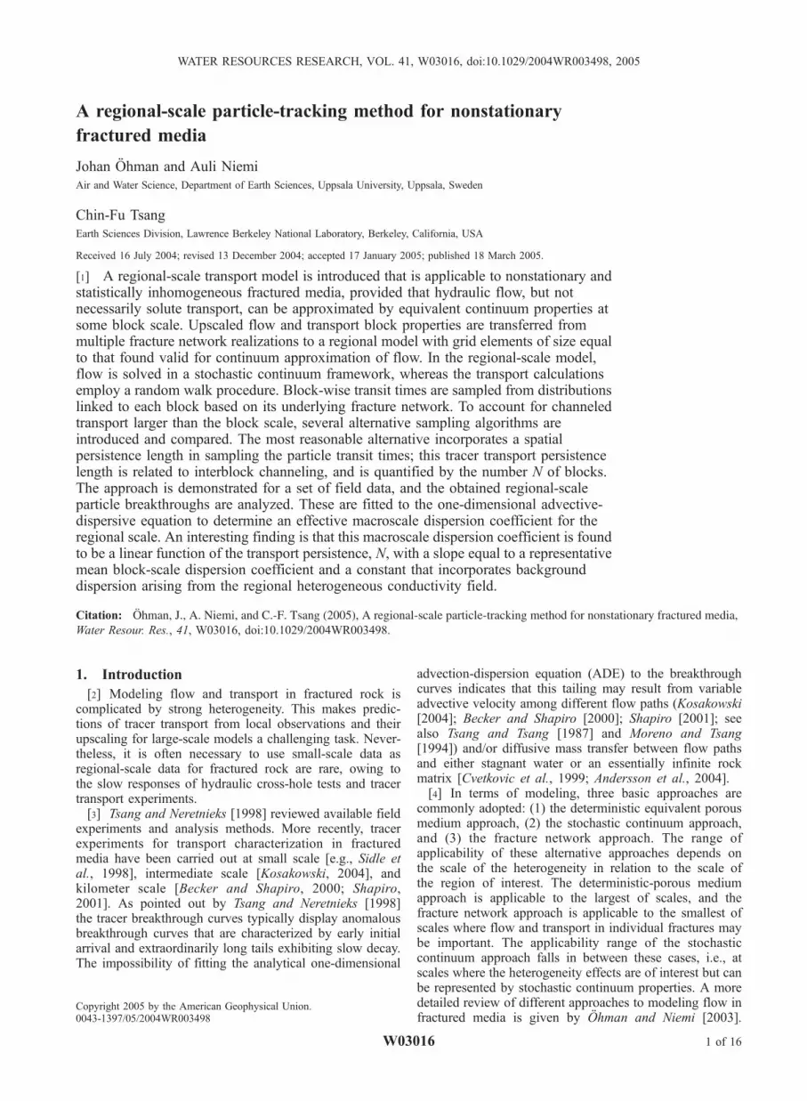
network realization i at the block scale, a large number ofparticles, typically 10,000, are released and their transit timedistributions gi(tp) are determined, where p refers to particlenumber. Because of the structure of the numerical simulatorused in the regional-scale model, separate transit timestatistics are needed for the ‘‘upstream’’ and ‘‘downstream’’sections of a fracture-network block. The reason for this isthat to attain consistency in the configuration of boundaryconditions for the integral finite difference model and forthe fracture network model, particles must move from onenodal point to another in the regional-scale model. Asexplained in section 2.3.2, these nodal points are locatedat the centers of numerical elements. Therefore transit timesare determined separately for the ‘‘upstream section’’ (i.e.,from the boundary with higher hydraulic head to the centerof the block) and for the ‘‘downstream section’’ (i.e., fromthe center of the block to the boundary with lower hydraulichead) and are denoted as At and Bt, respectively (Figure 1).Similarly as for upscaling conductivity, the particle-tracking

procedure is conducted for networks subject to fractureclosure of the stress regime at each depth interval, j.[23] The results are organized to enable a correct linkage

between block-scale transport properties and block conduc-tivities in the following regional-scale simulations. In otherwords, for each network realization i, we save the verticaland horizontal components of conductivity, Kiv and Kih, andfour distributions of transit times, giv(

Atp), giv(Btp), gih(

Atp),and gih(

Btp), and denote them with the same index i. Also,the calculated transit times in each distribution are ranked inascending order, from shortest transit time to longest, andgiven a rank m that varies from 1 to the total number ofparticles released (the smallest value of m corresponds to thefastest pathway and the largest m corresponds to the slowestpathway through the block element). The reason for savingthis information is that we shall use it to carry pathwayinformation between block elements in the regional-scaleparticle-tracking model, as will be explained later in section2.3.3. When this ranking m is discussed, we use the notationgi(

Atm) and gi(Btm).

2.3. Regional-Scale Stochastic Continuum Model

2.3.1. Stochastic Flow Model[24] Multiple stochastic continuum realizations of

regional-scale flow fields are generated based on conduc-tivity distributions at the block scale (section 2.2.1).These conductivity fields are correlated using an expo-nential variogram for borehole data that was upscaled tobe valid for block scale conductivity [Ohman et al.,2004]. Each block element in the regional model has aconductivity value Ki and is linked to its correspondingparticle transit time distribution gi(t). The regional-scaleflow fields are solved using the integral finite differencemethod. In this numerical method, property values arecalculated at nodal points located at the centers ofelements. This poses an additional complication whenimporting the upscaled values to the regional-scale model,because the transport between two nodal points actuallyinvolves properties of two block elements.2.3.2. Rules of Particle Movement[25] The particle transport in these regional-scale stochas-

tic continuum realizations is then modeled by first solvingthe flow fields and then releasing a large number of particles(we used 106) and observing their transport. The particlemovement is simulated according to the following:[26] 1. A particle moves from its present block element,

in direction k, to an adjacent element with probability, Pk,which is proportional to the outward directed flux in thatdirection, Qk

out, as defined by

Pk ¼Qout

kXk

Qoutk

; ð2Þ

wherePk

Qkout is the sum of all fluxes out of the element

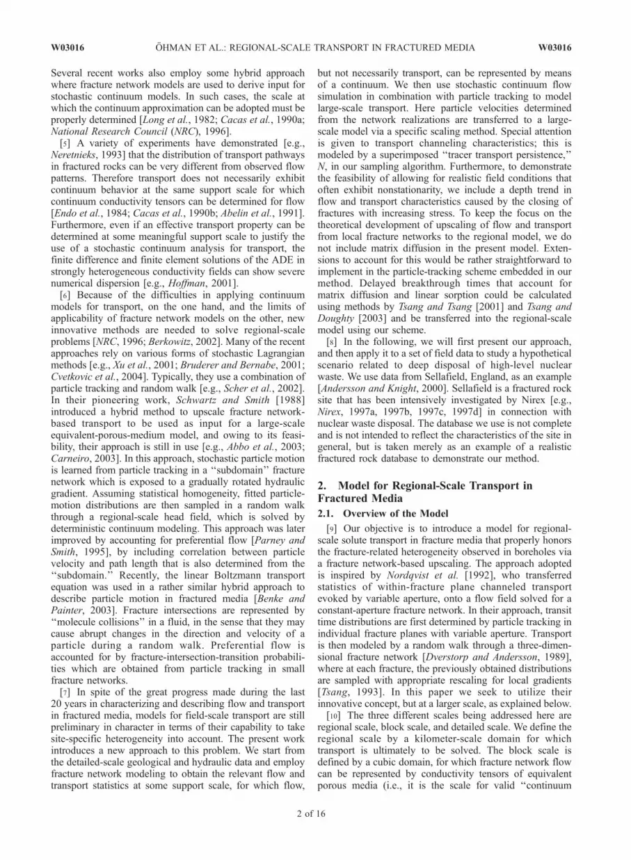
(Figure 2a).[27] 2. The particle first moves from the node situated at

the center of the present block element, through section B ofthat element, crosses the element interface, and movesthrough section A of an adjacent element, until it reachesthe neighboring element node (Figure 2b). Transport timesfor both sections (sections B and A0) are sampled from the

Figure 1. Geometry and boundary conditions of theblock-scale particle-tracking domain, divided into twohalves, an ‘‘upstream’’ section A and a ‘‘downstream’’section B, with imposed constant head boundary conditionsH0 > H1.

4 of 16


block-specific transit time distributions, gi(Btm) and

gi0(A0tm), associated with each element. The prescription

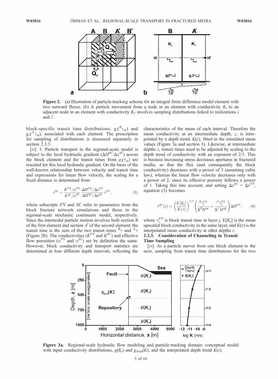
for sampling of distributions is discussed separately insection 2.3.3.[28] 3. Particle transport in the regional-scale model is

subject to the local hydraulic gradient (DHSC/DxSC) acrossthe block element and the transit times from gi(tm) arerescaled for this local hydraulic gradient. On the basis of thewell-known relationship between velocity and transit timeand expressions for linear flow velocity, the scaling for afixed distance is determined from

tSC ¼ KFN=fFN

KSC=fSC

DHFN=DxFN

DHSC=DxSCtFN ; ð3Þ

where subscripts FN and SC refer to parameters from theblock fracture network simulations and those in theregional-scale stochastic continuum model, respectively.Since the internodal particle motion involves both section Bof the first element and section A0 of the second element, thetransit time is the sum of the two transit times Bt and A0

t(Figure 2b). The conductivities (KFN and KSC) and effectiveflow porosities (fFN and fSC) are by definition the same.However, block conductivity and transport statistics aredetermined at four different depth intervals, reflecting the

characteristics of the mean of each interval. Therefore themean conductivity at an intermediate depth, z, is inter-polated by a depth trend, K(z), fitted to the simulated meanvalues (Figure 3a and section 3). Likewise, at intermediatedepths z, transit times need to be adjusted by scaling to thedepth trend of conductivity with an exponent of 2/3. Thisis because increasing stress decreases apertures in fracturedmedia, so that the flux (and consequently the blockconductivity) decreases with a power of 3 (assuming cubiclaw), whereas the linear flow velocity decreases only witha power of 2, since its effective porosity follows a powerof 1. Taking this into account, and setting DxSC = DxFN,equation (3) becomes

tSC zð Þ ¼E Kj

� �K zð Þ

� �2=3 BtFNjDBHSC

þA0tFNj

DA0HSC

!DHFN ; ð4Þ

where tjFN is block transit time in layer j, E[Kj] is the mean

upscaled block conductivity in the same layer, and K(z) is theinterpolated mean conductivity at other depths z.2.3.3. Consideration of Channeling in TransitTime Sampling[29] As a particle moves from one block element to the

next, sampling from transit time distributions for the two

Figure 2. (a) Illustration of particle-tracking scheme for an integral finite difference model element withtwo outward fluxes. (b) A particle movement from a node in an element with conductivity Ki to anadjacent node in an element with conductivity Ki0 involves sampling distributions linked to realizations iand i0.

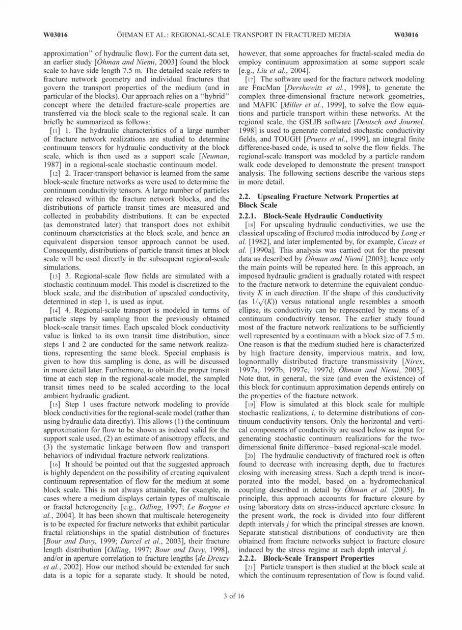
Figure 3a. Regional-scale hydraulic flow modeling and particle-tracking domain: conceptual modelwith input conductivity distributions, g(Kj) and g45m(K), and the interpolated depth trend K(z).


5 of 16

W03016

neighboring blocks are commonly assumed to be indepen-dent random processes. However, one could also expectsome correlation between neighboring elements, so thatparticles traveling along a fast path in one element wouldalso travel along a fast path in the next [cf. Parney andSmith, 1995; Benke and Painter, 2003]. In our model,spatial correlation is introduced into the regional stochasticconductivity field, but while this affects the regional-scaleflow field, it does not consider the possibility of channeledtransport pathways at the subblock scale persisting over adistance of several blocks.[30] To consider such a possibility, the block-scale

transit times (i.e., time from the inflow boundary to theoutflow boundary) are ranked from the slowest to thefastest, with index m ranging from 1 to 10,000, asdescribed earlier. In transit time sampling, possibilitiescan then range from autonomous random sampling withoutregard to the previous transit time, to a situation where mis maintained all along a regional particle trajectory. Thelatter implies that a particle which has followed a fasttrajectory in the previous block element also continueswith a fast trajectory in the next block element, and viceversa. Intermediate alternatives include allowing a smallchange in the rank, or introducing some type of transportpersistence length d where the rank is maintained only forthe distance d.[31] To implement this idea in the regional-scale simu-

lations, each particle is assigned an initial rank m at itsrelease, where m is randomly sampled from a uniformdistribution and used to identify a transit time in theblock-specific distributions. Given the particle rank in anupstream element being m, entering the next element theparticle is assigned a new rank m0; then the alternatives fordetermining m0 are given in Table 1.[32] The first alternative reflects a minimum level of

channeled transport, i.e., only the channeling arising from

the regional correlated conductivity field. This sampling isnot linked to previously sampled transit times for the blockelement; rather, the new rank m0 is randomly sampled froma uniform distribution.[33] The second alternative is the other extreme and

reflects the maximum level of channeled transport. Thesampling rank m randomly assigned to each particle at theonset is maintained during the entire particle trajectory andis used for selecting transit times in block-specific distribu-tions of each successive block element. Thus a particle borninto a fast or slow lane is kept on such, even though itsvelocity may vary along the route.[34] Neither of the two extremes above seems very

realistic, and hence two additional transitional concepts,the alternatives 3 and 4 in Table 1, are used to examineintermediate levels of transport channeling. These transi-tional concepts are based on alternative 2, but modified soas to introduce various levels of randomness, in order toregulate the level of transport channeling.[35] In alternative 3, the sampling rank is increased by

Dm (which can be positive or negative) each time a particlecrosses an element interface. The change Dm is determinedfrom a triangular probability distribution, which has anexpected value of zero and is bounded by a maximumchange, ±jDmmaxj. This maximum change, jDmmaxj, isvaried with values 0.01, 0.1, 0.25, 0.5, and 1.0 M, whereM is the maximum rank and thus represents high to lowlevels of channelized transport, respectively.[36] Alternative 4 in Table 1, is the case for ‘‘tracer-

transport persistence length’’ d, which is longer than theblock scale Dx, so that d = N � Dx, where we define N as‘‘tracer-transport persistence.’’ In this alternative, the sam-pling rank m is kept fixed over a distance of N successiveelements. After N elements have been traversed, a new rankm0 is sampled independently, as in alternative 1. The particlethen moves along the next set of N successive block

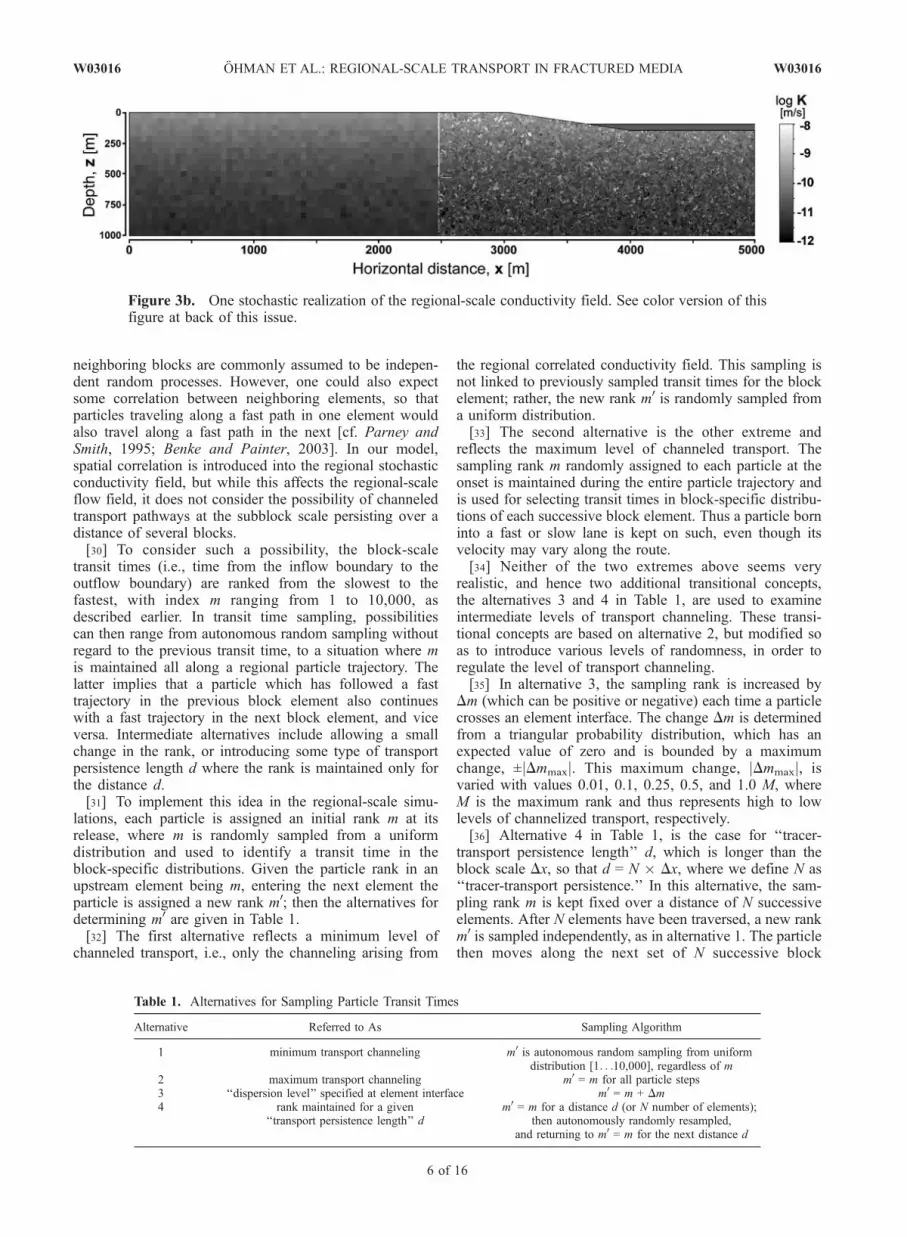
Figure 3b. One stochastic realization of the regional-scale conductivity field. See color version of thisfigure at back of this issue.

Table 1. Alternatives for Sampling Particle Transit Times

Alternative Referred to As Sampling Algorithm

1 minimum transport channeling m0 is autonomous random sampling from uniformdistribution [1. . .10,000], regardless of m

2 maximum transport channeling m0 = m for all particle steps3 ‘‘dispersion level’’ specified at element interface m0 = m + Dm4 rank maintained for a given

‘‘transport persistence length’’ dm0 = m for a distance d (or N number of elements);

then autonomously randomly resampled,and returning to m0 = m for the next distance d

6 of 16


elements with a fixed m value. For a given simulation ofregional tracer transport (106 particles), N is treated as arandom variable sampled from a uniform distribution,ranging from 1 to 2N*A 1, with mean N*A. However, toavoid cases where a choice of N steps would lead theparticle to go beyond the exit boundary, N is cut back sothat it always ends at the boundary. Thus the mean of therandom N values, NA, is always less than intended for largecases of N*A. Channelized transport is examined for variousaverage ‘‘transport persistence,’’ NA, ranging from 390.4 to1.0, which represent maximum to minimum channelinglevels, respectively.

3. Example Application to Field Data

[37] The use of the model developed is demonstratedas part of a model cross-comparison study within theinternational DECOVALEX project [Tsang et al., 2004].The database used for this comes from the Sellafield sitein England, as summarized by Andersson and Knight[2000]. Particle transport from a potential deep nuclearwaste repository is simulated in a vertical cross section(Figure 3a). The range of particle transit times from theunderground repository to the sea is to be simulated.No-flow boundaries are assigned at x = 5000 m, x = 0 m,based on symmetry considerations at water divide, and atz = 1000 m, based on the very low conductivity at thisdepth, as often assumed in fractured media. Constant-head boundary conditions are assigned at the top of themodel, corresponding to the mean levels of the ground-water table and the sea. Other than a vertical fault in themiddle of the domain, the medium is ‘‘average’’ fracturedrock. This rock also has a depth trend in conductivitycaused by fractures closing depth increases. It is thehydraulic and transport properties of this ‘‘average’’ frac-tured rock that need upscaling for the regional-scaletransport model. Because of the domain geometry, theseproperties are characterized at four depth levels (e.g., g(Kj)where j refers to the depth level in Figure 3a), and at alarger support scale in a region having less influence ontransport (e.g., g45m(K)), which will be explained in thefollowing sections.

3.1. Upscaling of Fracture Networks

3.1.1. Data[38] Our approach is based on three-dimensional fracture

network modeling at the block scale. Multiple frac-ture network realizations are generated, and input data forthese network realizations are statistical distributions ofgeologically observed fracture orientations, lengths, density,and intersection termination percentage, taken from theNirex databases as summarized by Andersson and Knight[2000]. Statistical fracture transmissivity distributions areestimated using a probabilistic analysis of hydraulic welltest data, according to the method introduced by Osnes et al.[1988]. Details of these fracture and hydraulic conductivitydata and their analysis for hydraulic fracture networkmodeling are given by Ohman and Niemi [2003] and willnot be repeated here.[39] To account for decreasing conductivity with depth,

principal stresses, as reported by Nirex [1997d], are used tocalculate the stress regimes at various depths. These in turn

are used to calculate the fracture transmissivities at thesedepths, as hydraulic data are only available at a limiteddepth interval (from 635 to 790 m). In doing so, fracturetransmissivities are adjusted, such that the relation betweenfracture aperture and the stress-regime satisfies an empiricalfracture-closure relationship based on an analysis of coreloading-unloading data. These latter data come fromNorwegian Geotechnical Institute (NGI) [1993]. The stepof adjusting fracture transmissivity depending on its orien-tation in an ambient stress-field is further explained byOhman et al. [2005].3.1.2. Hydraulic Upscaling at Block Scale[40] Block-scale flow modeling was conducted for 4 �

100 ( j � i) fracture network realizations to generatehydraulic conductivity distributions as input to the two-dimensional regional-scale flow calculations. The simula-tions were carried out as discussed in section 2.3.1 and arefurther described by Ohman and Niemi [2003]. Thehorizontal and vertical components of equivalent conduc-tivity were extracted from each simulated conductivitytensor to form input conductivity distributions for gener-ating the regional-scale stochastic continuum flow model.Four different block-scale conductivity distributions weredetermined, g(Kj), which correspond to the four differentdepth levels j = 100, 400, 713, and 1000 m.[41] For computational reasons, a statistical conductivity

distribution was also determined at 45-m block scale,g45m(K). This distribution is intended for regions wherethe heterogeneity effects are of less importance (Figures 3aand 3b) because particles are not expected to pass throughthem. For this reason, an additional upscaling was carriedout to further upscale the 7.5-m scale conductivities toeffective conductivities at 45-m scale. This upscaling wasbased on stochastic continuum modeling and is presented indetail by Ohman et al. [2004].3.1.3. Testing for Continuum Dispersivity atBlock Scale[42] First, to establish the necessity of our random

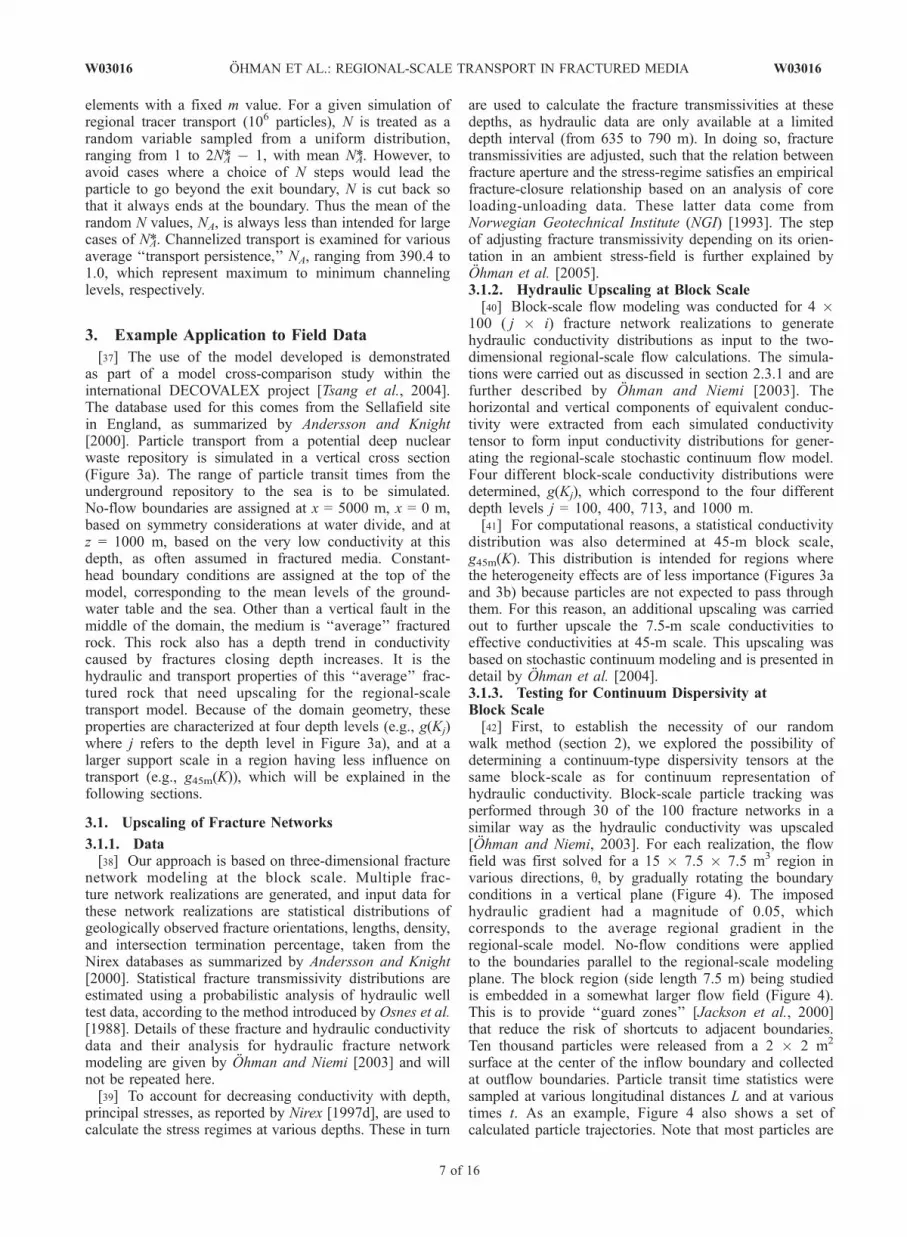
walk method (section 2), we explored the possibility ofdetermining a continuum-type dispersivity tensors at thesame block-scale as for continuum representation ofhydraulic conductivity. Block-scale particle tracking wasperformed through 30 of the 100 fracture networks in asimilar way as the hydraulic conductivity was upscaled[Ohman and Niemi, 2003]. For each realization, the flowfield was first solved for a 15 � 7.5 � 7.5 m3 region invarious directions, q, by gradually rotating the boundaryconditions in a vertical plane (Figure 4). The imposedhydraulic gradient had a magnitude of 0.05, whichcorresponds to the average regional gradient in theregional-scale model. No-flow conditions were appliedto the boundaries parallel to the regional-scale modelingplane. The block region (side length 7.5 m) being studiedis embedded in a somewhat larger flow field (Figure 4).This is to provide ‘‘guard zones’’ [Jackson et al., 2000]that reduce the risk of shortcuts to adjacent boundaries.Ten thousand particles were released from a 2 � 2 m2

surface at the center of the inflow boundary and collectedat outflow boundaries. Particle transit time statistics weresampled at various longitudinal distances L and at varioustimes t. As an example, Figure 4 also shows a set ofcalculated particle trajectories. Note that most particles are


7 of 16

W03016

channeled along a high-velocity path and generate transittimes around 30 years, whereas for others it can exceed80 years.[43] The results of this study showed, in agreement with

earlier studies, for example, of Endo et al. [1984], that thesimulated particle breakthroughs were much more hetero-geneous than the results from the corresponding flowsimulations. On the basis of two criteria for the validity ofcontinuum behavior for transport (section 2.2.2), none ofthe 30 fracture networks examined could be classified as acontinuum-type medium for transport.[44] As an example, the obtained transit time percentiles,

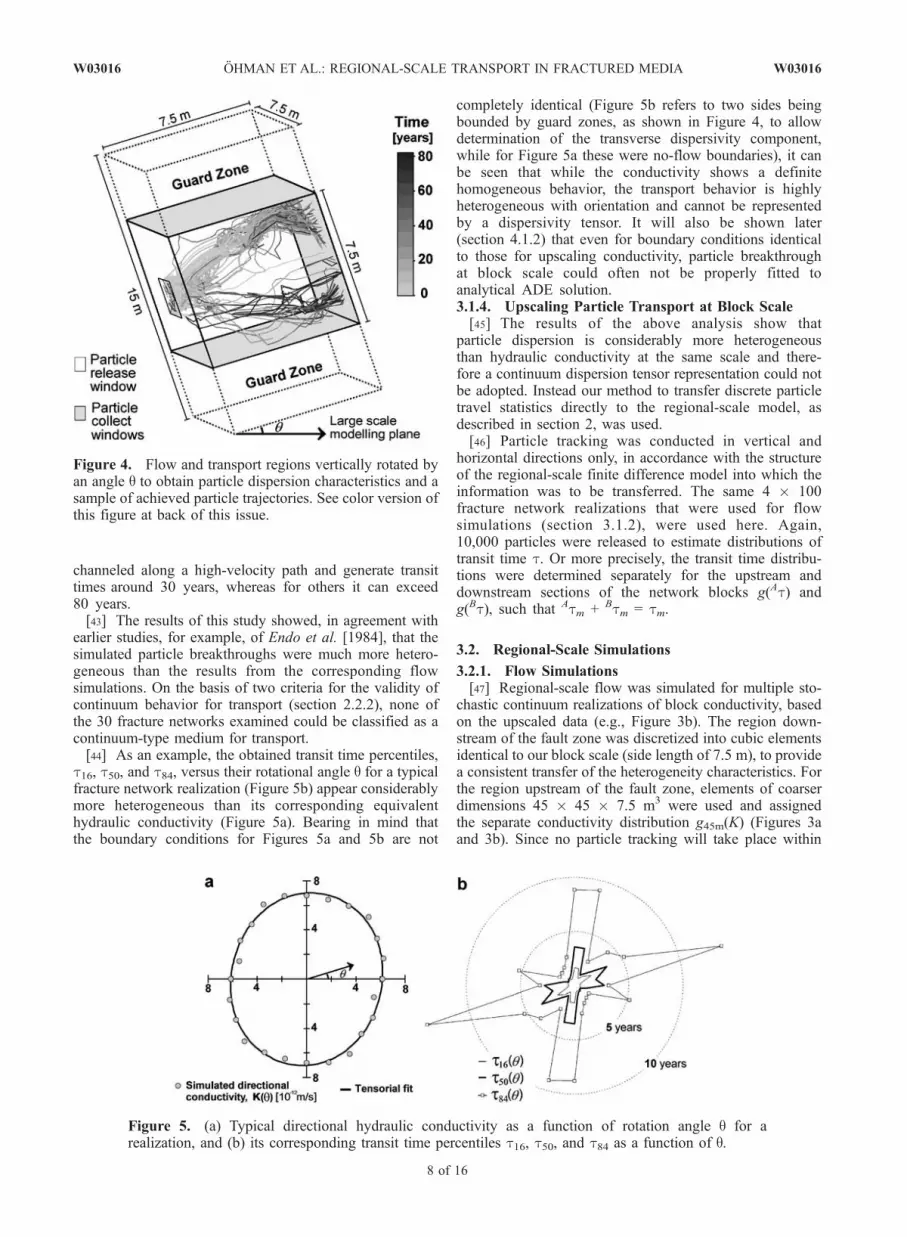
t16, t50, and t84, versus their rotational angle q for a typicalfracture network realization (Figure 5b) appear considerablymore heterogeneous than its corresponding equivalenthydraulic conductivity (Figure 5a). Bearing in mind thatthe boundary conditions for Figures 5a and 5b are not

completely identical (Figure 5b refers to two sides beingbounded by guard zones, as shown in Figure 4, to allowdetermination of the transverse dispersivity component,while for Figure 5a these were no-flow boundaries), it canbe seen that while the conductivity shows a definitehomogeneous behavior, the transport behavior is highlyheterogeneous with orientation and cannot be representedby a dispersivity tensor. It will also be shown later(section 4.1.2) that even for boundary conditions identicalto those for upscaling conductivity, particle breakthroughat block scale could often not be properly fitted toanalytical ADE solution.3.1.4. Upscaling Particle Transport at Block Scale[45] The results of the above analysis show that

particle dispersion is considerably more heterogeneousthan hydraulic conductivity at the same scale and there-fore a continuum dispersion tensor representation could notbe adopted. Instead our method to transfer discrete particletravel statistics directly to the regional-scale model, asdescribed in section 2, was used.[46] Particle tracking was conducted in vertical and

horizontal directions only, in accordance with the structureof the regional-scale finite difference model into which theinformation was to be transferred. The same 4 � 100fracture network realizations that were used for flowsimulations (section 3.1.2), were used here. Again,10,000 particles were released to estimate distributions oftransit time t. Or more precisely, the transit time distribu-tions were determined separately for the upstream anddownstream sections of the network blocks g(At) andg(Bt), such that Atm + Btm = tm.

3.2. Regional-Scale Simulations

3.2.1. Flow Simulations[47] Regional-scale flow was simulated for multiple sto-

chastic continuum realizations of block conductivity, basedon the upscaled data (e.g., Figure 3b). The region down-stream of the fault zone was discretized into cubic elementsidentical to our block scale (side length of 7.5 m), to providea consistent transfer of the heterogeneity characteristics. Forthe region upstream of the fault zone, elements of coarserdimensions 45 � 45 � 7.5 m3 were used and assignedthe separate conductivity distribution g45m(K) (Figures 3aand 3b). Since no particle tracking will take place within

Figure 4. Flow and transport regions vertically rotated byan angle q to obtain particle dispersion characteristics and asample of achieved particle trajectories. See color version ofthis figure at back of this issue.

Figure 5. (a) Typical directional hydraulic conductivity as a function of rotation angle q for arealization, and (b) its corresponding transit time percentiles t16, t50, and t84 as a function of q.

8 of 16


this region, the particle transport characteristics were notupscaled to this support scale.[48] First, four correlated stochastic conductivity fields

for the region were generated for the four different depthintervals (0–250, 250–550, 550–856, and 856–1000 m),using the upscaled conductivity statistics g(Kj) and anexponential variogram with a correlation length of 18 m,based on a separate variogram upscaling study presented byOhman et al. [2004]. Then, the mean conductivity of thefields was adjusted to the interpolated depth trend, K(z) inFigure 3a, to obtain smoothly varying mean conductivity atall intermediate depths, z. Finally, each generated conduc-tivity value was indexed to its actual network realization oforigin, in order to link each element to its correspondingparticle transit time distribution. The procedure describedwas repeated, and 30 regional-scale realizations were gen-erated. Then the steady state flow field was solved for each.3.2.2. Regional-Scale Particle Tracking[49] Regional-scale particle tracking was then carried out

for steady state flow fields of the 30 realizations. For eachrealization, 106 particles were released at the repository(Figure 3a), and their breakthrough at the sea was observedand analyzed. The impact of different levels of superim-posed channelized transport, represented by the four alter-natives in the sampling algorithms (Table 1, section 2.3.3),was then explored.

4. Results

4.1. Upscaling Network Characteristics

[50] The results of upscaling the flow in the block-scalefracture networks are discussed in detail by Ohman andNiemi [2003] and will not be repeated here. Those resultsshowed that most block conductivities could be reasonablywell represented by means of a continuum conductivitytensor at the 7.5-m block scale. The criterion for thiswas that the directional conductivity as a function oforientation must smoothly follow the transformation of atensor [Harrison and Hudson, 2000].4.1.1. Particle Transit Time Distributions[51] A conclusion drawn in the previous section was

that solute transport cannot be represented by means of

dispersion tensors at the 7.5-m block scale. Thus weemploy our approach to transfer particle transit times fromfracture networks to the regional-scale model with the useof block-scale distributions.[52] Inspection of the results shows that the transit

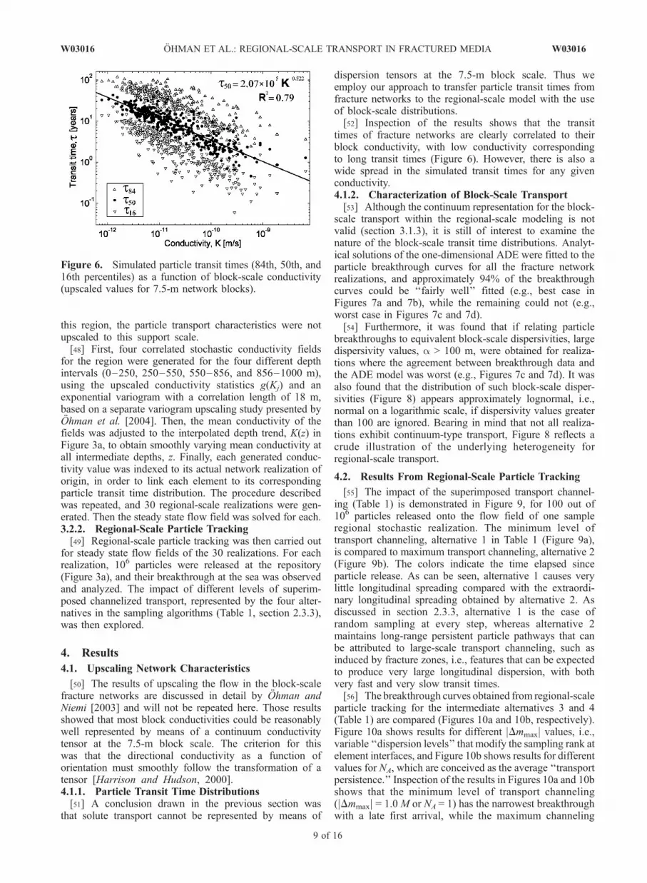
times of fracture networks are clearly correlated to theirblock conductivity, with low conductivity correspondingto long transit times (Figure 6). However, there is also awide spread in the simulated transit times for any givenconductivity.4.1.2. Characterization of Block-Scale Transport[53] Although the continuum representation for the block-

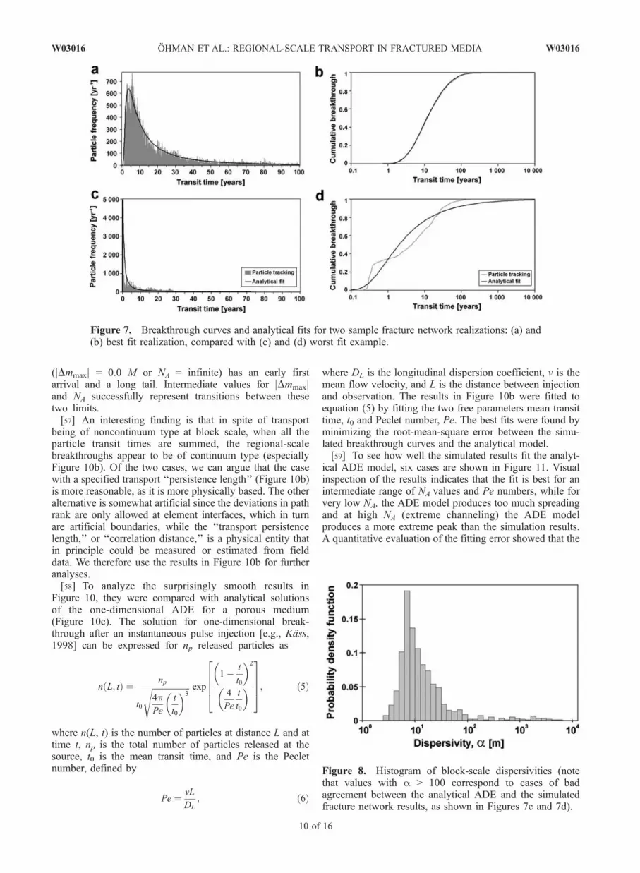
scale transport within the regional-scale modeling is notvalid (section 3.1.3), it is still of interest to examine thenature of the block-scale transit time distributions. Analyt-ical solutions of the one-dimensional ADE were fitted to theparticle breakthrough curves for all the fracture networkrealizations, and approximately 94% of the breakthroughcurves could be ‘‘fairly well’’ fitted (e.g., best case inFigures 7a and 7b), while the remaining could not (e.g.,worst case in Figures 7c and 7d).[54] Furthermore, it was found that if relating particle

breakthroughs to equivalent block-scale dispersivities, largedispersivity values, a > 100 m, were obtained for realiza-tions where the agreement between breakthrough data andthe ADE model was worst (e.g., Figures 7c and 7d). It wasalso found that the distribution of such block-scale disper-sivities (Figure 8) appears approximately lognormal, i.e.,normal on a logarithmic scale, if dispersivity values greaterthan 100 are ignored. Bearing in mind that not all realiza-tions exhibit continuum-type transport, Figure 8 reflects acrude illustration of the underlying heterogeneity forregional-scale transport.

4.2. Results From Regional-Scale Particle Tracking

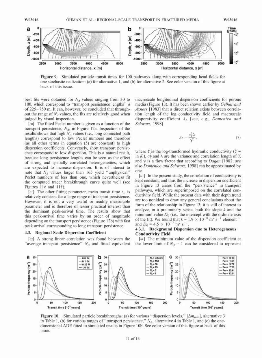
[55] The impact of the superimposed transport channel-ing (Table 1) is demonstrated in Figure 9, for 100 out of106 particles released onto the flow field of one sampleregional stochastic realization. The minimum level oftransport channeling, alternative 1 in Table 1 (Figure 9a),is compared to maximum transport channeling, alternative 2(Figure 9b). The colors indicate the time elapsed sinceparticle release. As can be seen, alternative 1 causes verylittle longitudinal spreading compared with the extraordi-nary longitudinal spreading obtained by alternative 2. Asdiscussed in section 2.3.3, alternative 1 is the case ofrandom sampling at every step, whereas alternative 2maintains long-range persistent particle pathways that canbe attributed to large-scale transport channeling, such asinduced by fracture zones, i.e., features that can be expectedto produce very large longitudinal dispersion, with bothvery fast and very slow transit times.[56] The breakthrough curves obtained from regional-scale

particle tracking for the intermediate alternatives 3 and 4(Table 1) are compared (Figures 10a and 10b, respectively).Figure 10a shows results for different jDmmaxj values, i.e.,variable ‘‘dispersion levels’’ that modify the sampling rank atelement interfaces, and Figure 10b shows results for differentvalues for NA, which are conceived as the average ‘‘transportpersistence.’’ Inspection of the results in Figures 10a and 10bshows that the minimum level of transport channeling(jDmmaxj = 1.0M or NA = 1) has the narrowest breakthroughwith a late first arrival, while the maximum channeling

Figure 6. Simulated particle transit times (84th, 50th, and16th percentiles) as a function of block-scale conductivity(upscaled values for 7.5-m network blocks).


9 of 16

W03016

(jDmmaxj = 0.0 M or NA = infinite) has an early firstarrival and a long tail. Intermediate values for jDmmaxjand NA successfully represent transitions between thesetwo limits.[57] An interesting finding is that in spite of transport

being of noncontinuum type at block scale, when all theparticle transit times are summed, the regional-scalebreakthroughs appear to be of continuum type (especiallyFigure 10b). Of the two cases, we can argue that the casewith a specified transport ‘‘persistence length’’ (Figure 10b)is more reasonable, as it is more physically based. The otheralternative is somewhat artificial since the deviations in pathrank are only allowed at element interfaces, which in turnare artificial boundaries, while the ‘‘transport persistencelength,’’ or ‘‘correlation distance,’’ is a physical entity thatin principle could be measured or estimated from fielddata. We therefore use the results in Figure 10b for furtheranalyses.[58] To analyze the surprisingly smooth results in

Figure 10, they were compared with analytical solutionsof the one-dimensional ADE for a porous medium(Figure 10c). The solution for one-dimensional break-through after an instantaneous pulse injection [e.g., Kass,1998] can be expressed for np released particles as

n L; tð Þ ¼ np

t0

ffiffiffiffiffiffiffiffiffiffiffiffiffiffiffiffiffiffiffi4pPe

t

t0

� �3s exp

1 t

t0

� �2

4

Pe

t

t0

� �26664

37775; ð5Þ

where n(L, t) is the number of particles at distance L and attime t, np is the total number of particles released at thesource, t0 is the mean transit time, and Pe is the Pecletnumber, defined by

Pe ¼ vL

DL

; ð6Þ

where DL is the longitudinal dispersion coefficient, v is themean flow velocity, and L is the distance between injectionand observation. The results in Figure 10b were fitted toequation (5) by fitting the two free parameters mean transittime, t0 and Peclet number, Pe. The best fits were found byminimizing the root-mean-square error between the simu-lated breakthrough curves and the analytical model.[59] To see how well the simulated results fit the analyt-

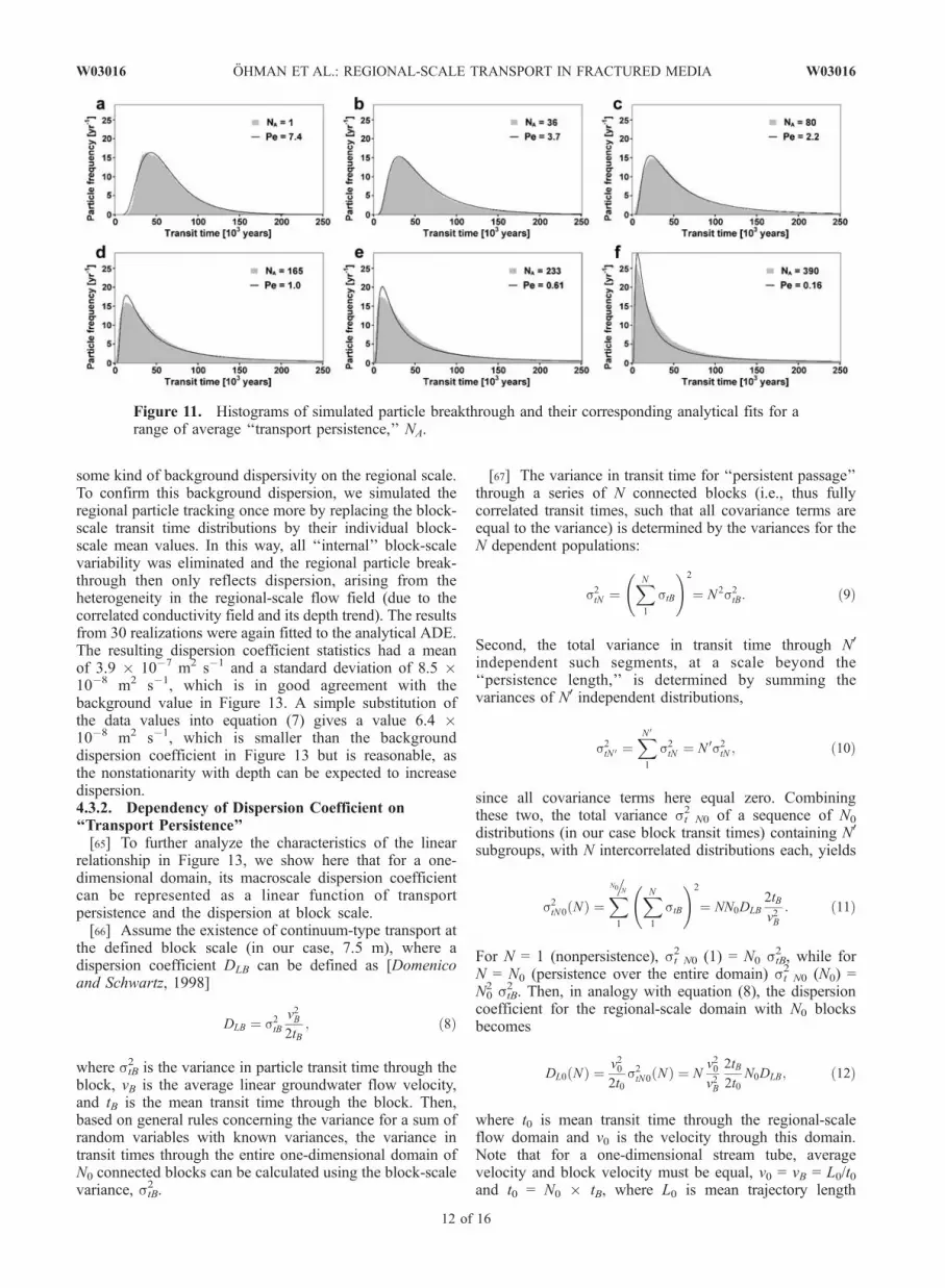
ical ADE model, six cases are shown in Figure 11. Visualinspection of the results indicates that the fit is best for anintermediate range of NA values and Pe numbers, while forvery low NA, the ADE model produces too much spreadingand at high NA (extreme channeling) the ADE modelproduces a more extreme peak than the simulation results.A quantitative evaluation of the fitting error showed that the

Figure 7. Breakthrough curves and analytical fits for two sample fracture network realizations: (a) and(b) best fit realization, compared with (c) and (d) worst fit example.

Figure 8. Histogram of block-scale dispersivities (notethat values with a > 100 correspond to cases of badagreement between the analytical ADE and the simulatedfracture network results, as shown in Figures 7c and 7d).

10 of 16


best fits were obtained for NA values ranging from 30 to100, which correspond to ‘‘transport persistence lengths’’ dof 225–750 m. It can, however, be concluded that through-out the range of NA values, the fits are relatively good whenjudged by visual inspection.[60] The fitted Peclet number is given as a function of the

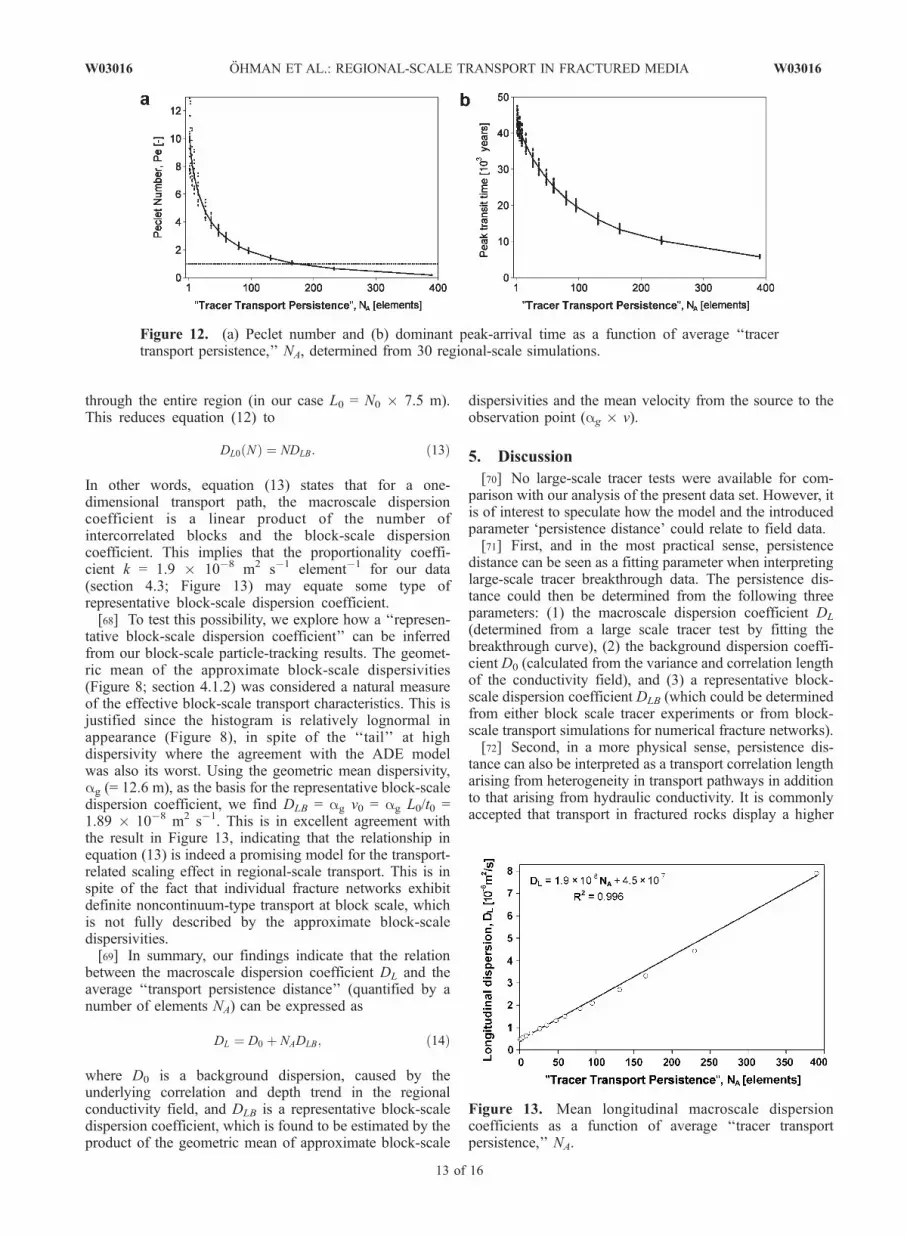
transport persistence, NA, in Figure 12a. Inspection of theresults shows that high NA values (i.e., long connected pathlengths) correspond to low Peclet numbers and therefore(as all other terms in equation (5) are constant) to highdispersion coefficients. Conversely, short transport persist-ence correspond to low dispersion. This is a natural result,because long persistence lengths can be seen as the effectof strong and spatially correlated heterogeneities, whichare expected to increase dispersion. It is of interest tonote that NA values larger than 165 yield ‘‘unphysical’’Peclet numbers of less than one, which nevertheless fitthe computed tracer breakthrough curve quite well (seeFigures 11e and 11f ).[61] The other fitting parameter, mean transit time t0, is

relatively constant for a large range of transport persistence.However, it is not a very useful or readily measurableparameter and is therefore of lesser practical interest thanthe dominant peak-arrival time. The results show thatthis peak-arrival time varies by an order of magnitudedepending on the transport persistence (Figure 12b) with fastpeak arrival corresponding to long transport persistence.

4.3. Regional-Scale Dispersion Coefficient

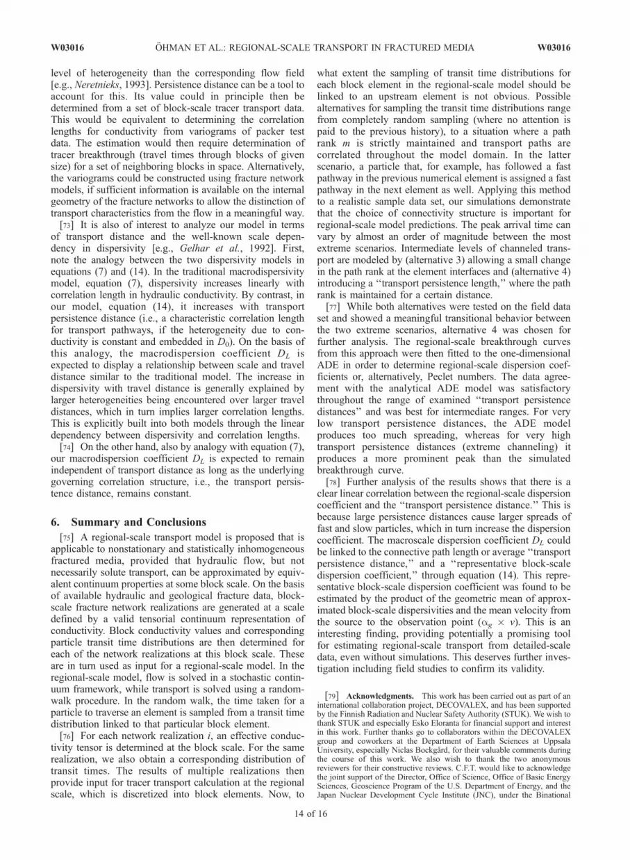
[62] A strong linear correlation was found between the‘‘average transport persistence’’ NA and fitted equivalent

macroscale longitudinal dispersion coefficients for porousmedia (Figure 13). It has been shown earlier by Gelhar andAxness [1983] that a direct relation exists between correla-tion length of the log conductivity field and macroscaledispersivity coefficient AL [see, e.g., Domenico andSchwarz, 1998]

AL ¼ s2Ylg2

; ð7Þ

where Y is the log-transformed hydraulic conductivity (Y =ln K ), sY

2 and l are the variance and correlation length of Y,and g is a flow factor that according to Dagan [1982; seealso Domenico and Schwarz, 1998] can be approximated byone.[63] In the present study, the correlation of conductivity is

kept constant, and thus the increase in dispersion coefficientin Figure 13 arises from the ‘‘persistence’’ in transportpathways, which are superimposed on the correlated con-ductivity field. While the present data with their depth trendare too nonideal to draw any general conclusions about theform of the relationship in Figure 13, it is still of interest toanalyze, in a preliminary sense, both the slope k and theminimum value D0 (i.e., the intercept with the ordinate axisof the fit). We found that k = 1.9 � 108 m2 s1 element1

and D0 = 4.5 � 107 m2 s1.4.3.1. Background Dispersion due to HeterogeneousConductivity Field[64] The minimum value of the dispersion coefficient at

the lower limit of NA = 1 can be considered to represent

Figure 9. Simulated particle transit times for 100 pathways along with corresponding head fields forone stochastic realization: (a) for alternative 1, and (b) for alternative 2. See color version of this figure atback of this issue.

Figure 10. Simulated particle breakthroughs: (a) for various ‘‘dispersion levels,’’ jDmmaxj, alternative 3in Table 1, (b) for various ranges of ‘‘transport persistence,’’ NA, alternative 4 in Table 1, and (c) the one-dimensional ADE fitted to simulated results in Figure 10b. See color version of this figure at back of thisissue.


11 of 16

W03016

some kind of background dispersivity on the regional scale.To confirm this background dispersion, we simulated theregional particle tracking once more by replacing the block-scale transit time distributions by their individual block-scale mean values. In this way, all ‘‘internal’’ block-scalevariability was eliminated and the regional particle break-through then only reflects dispersion, arising from theheterogeneity in the regional-scale flow field (due to thecorrelated conductivity field and its depth trend). The resultsfrom 30 realizations were again fitted to the analytical ADE.The resulting dispersion coefficient statistics had a meanof 3.9 � 107 m2 s1 and a standard deviation of 8.5 �108 m2 s1, which is in good agreement with thebackground value in Figure 13. A simple substitution ofthe data values into equation (7) gives a value 6.4 �108 m2 s1, which is smaller than the backgrounddispersion coefficient in Figure 13 but is reasonable, asthe nonstationarity with depth can be expected to increasedispersion.4.3.2. Dependency of Dispersion Coefficient on‘‘Transport Persistence’’[65] To further analyze the characteristics of the linear

relationship in Figure 13, we show here that for a one-dimensional domain, its macroscale dispersion coefficientcan be represented as a linear function of transportpersistence and the dispersion at block scale.[66] Assume the existence of continuum-type transport at

the defined block scale (in our case, 7.5 m), where adispersion coefficient DLB can be defined as [Domenicoand Schwartz, 1998]

DLB ¼ s2tBv2B2tB

; ð8Þ

where stB2 is the variance in particle transit time through the

block, vB is the average linear groundwater flow velocity,and tB is the mean transit time through the block. Then,based on general rules concerning the variance for a sum ofrandom variables with known variances, the variance intransit times through the entire one-dimensional domain ofN0 connected blocks can be calculated using the block-scalevariance, stB

2 .

[67] The variance in transit time for ‘‘persistent passage’’through a series of N connected blocks (i.e., thus fullycorrelated transit times, such that all covariance terms areequal to the variance) is determined by the variances for theN dependent populations:

s2tN ¼XN1

stB

!2

¼ N2s2tB: ð9Þ

Second, the total variance in transit time through N0

independent such segments, at a scale beyond the‘‘persistence length,’’ is determined by summing thevariances of N0 independent distributions,

s2tN 0 ¼XN 0

1

s2tN ¼ N 0s2tN ; ð10Þ

since all covariance terms here equal zero. Combiningthese two, the total variance st N0

2 of a sequence of N0

distributions (in our case block transit times) containing N0

subgroups, with N intercorrelated distributions each, yields

s2tN0 Nð Þ ¼XN0�N1

XN1

stB

!2

¼ NN0DLB

2tB

v2B: ð11Þ

For N = 1 (nonpersistence), st N02 (1) = N0 stB

2 , while forN = N0 (persistence over the entire domain) st N0

2 (N0) =N02 stB

2 . Then, in analogy with equation (8), the dispersioncoefficient for the regional-scale domain with N0 blocksbecomes

DL0 Nð Þ ¼ v202t0

s2tN0 Nð Þ ¼ Nv20v2B

2tB

2t0N0DLB; ð12Þ

where t0 is mean transit time through the regional-scaleflow domain and v0 is the velocity through this domain.Note that for a one-dimensional stream tube, averagevelocity and block velocity must be equal, v0 = vB = L0/t0and t0 = N0 � tB, where L0 is mean trajectory length

Figure 11. Histograms of simulated particle breakthrough and their corresponding analytical fits for arange of average ‘‘transport persistence,’’ NA.

12 of 16


through the entire region (in our case L0 = N0 � 7.5 m).This reduces equation (12) to

DL0 Nð Þ ¼ NDLB: ð13Þ

In other words, equation (13) states that for a one-dimensional transport path, the macroscale dispersioncoefficient is a linear product of the number ofintercorrelated blocks and the block-scale dispersioncoefficient. This implies that the proportionality coeffi-cient k = 1.9 � 108 m2 s1 element1 for our data(section 4.3; Figure 13) may equate some type ofrepresentative block-scale dispersion coefficient.[68] To test this possibility, we explore how a ‘‘represen-

tative block-scale dispersion coefficient’’ can be inferredfrom our block-scale particle-tracking results. The geomet-ric mean of the approximate block-scale dispersivities(Figure 8; section 4.1.2) was considered a natural measureof the effective block-scale transport characteristics. This isjustified since the histogram is relatively lognormal inappearance (Figure 8), in spite of the ‘‘tail’’ at highdispersivity where the agreement with the ADE modelwas also its worst. Using the geometric mean dispersivity,ag (= 12.6 m), as the basis for the representative block-scaledispersion coefficient, we find DLB = ag v0 = ag L0/t0 =1.89 � 108 m2 s1. This is in excellent agreement withthe result in Figure 13, indicating that the relationship inequation (13) is indeed a promising model for the transport-related scaling effect in regional-scale transport. This is inspite of the fact that individual fracture networks exhibitdefinite noncontinuum-type transport at block scale, whichis not fully described by the approximate block-scaledispersivities.[69] In summary, our findings indicate that the relation

between the macroscale dispersion coefficient DL and theaverage ‘‘transport persistence distance’’ (quantified by anumber of elements NA) can be expressed as

DL ¼ D0 þ NADLB; ð14Þ

where D0 is a background dispersion, caused by theunderlying correlation and depth trend in the regionalconductivity field, and DLB is a representative block-scaledispersion coefficient, which is found to be estimated by theproduct of the geometric mean of approximate block-scale

dispersivities and the mean velocity from the source to theobservation point (ag � v).

5. Discussion

[70] No large-scale tracer tests were available for com-parison with our analysis of the present data set. However, itis of interest to speculate how the model and the introducedparameter ‘persistence distance’ could relate to field data.[71] First, and in the most practical sense, persistence

distance can be seen as a fitting parameter when interpretinglarge-scale tracer breakthrough data. The persistence dis-tance could then be determined from the following threeparameters: (1) the macroscale dispersion coefficient DL

(determined from a large scale tracer test by fitting thebreakthrough curve), (2) the background dispersion coeffi-cient D0 (calculated from the variance and correlation lengthof the conductivity field), and (3) a representative block-scale dispersion coefficient DLB (which could be determinedfrom either block scale tracer experiments or from block-scale transport simulations for numerical fracture networks).[72] Second, in a more physical sense, persistence dis-

tance can also be interpreted as a transport correlation lengtharising from heterogeneity in transport pathways in additionto that arising from hydraulic conductivity. It is commonlyaccepted that transport in fractured rocks display a higher

Figure 12. (a) Peclet number and (b) dominant peak-arrival time as a function of average ‘‘tracertransport persistence,’’ NA, determined from 30 regional-scale simulations.

Figure 13. Mean longitudinal macroscale dispersioncoefficients as a function of average ‘‘tracer transportpersistence,’’ NA.


13 of 16

W03016

level of heterogeneity than the corresponding flow field[e.g., Neretnieks, 1993]. Persistence distance can be a tool toaccount for this. Its value could in principle then bedetermined from a set of block-scale tracer transport data.This would be equivalent to determining the correlationlengths for conductivity from variograms of packer testdata. The estimation would then require determination oftracer breakthrough (travel times through blocks of givensize) for a set of neighboring blocks in space. Alternatively,the variograms could be constructed using fracture networkmodels, if sufficient information is available on the internalgeometry of the fracture networks to allow the distinction oftransport characteristics from the flow in a meaningful way.[73] It is also of interest to analyze our model in terms

of transport distance and the well-known scale depen-dency in dispersivity [e.g., Gelhar et al., 1992]. First,note the analogy between the two dispersivity models inequations (7) and (14). In the traditional macrodispersivitymodel, equation (7), dispersivity increases linearly withcorrelation length in hydraulic conductivity. By contrast, inour model, equation (14), it increases with transportpersistence distance (i.e., a characteristic correlation lengthfor transport pathways, if the heterogeneity due to con-ductivity is constant and embedded in D0). On the basis ofthis analogy, the macrodispersion coefficient DL isexpected to display a relationship between scale and traveldistance similar to the traditional model. The increase indispersivity with travel distance is generally explained bylarger heterogeneities being encountered over larger traveldistances, which in turn implies larger correlation lengths.This is explicitly built into both models through the lineardependency between dispersivity and correlation lengths.[74] On the other hand, also by analogy with equation (7),

our macrodispersion coefficient DL is expected to remainindependent of transport distance as long as the underlyinggoverning correlation structure, i.e., the transport persis-tence distance, remains constant.

6. Summary and Conclusions

[75] A regional-scale transport model is proposed that isapplicable to nonstationary and statistically inhomogeneousfractured media, provided that hydraulic flow, but notnecessarily solute transport, can be approximated by equiv-alent continuum properties at some block scale. On the basisof available hydraulic and geological fracture data, block-scale fracture network realizations are generated at a scaledefined by a valid tensorial continuum representation ofconductivity. Block conductivity values and correspondingparticle transit time distributions are then determined foreach of the network realizations at this block scale. Theseare in turn used as input for a regional-scale model. In theregional-scale model, flow is solved in a stochastic contin-uum framework, while transport is solved using a random-walk procedure. In the random walk, the time taken for aparticle to traverse an element is sampled from a transit timedistribution linked to that particular block element.[76] For each network realization i, an effective conduc-

tivity tensor is determined at the block scale. For the samerealization, we also obtain a corresponding distribution oftransit times. The results of multiple realizations thenprovide input for tracer transport calculation at the regionalscale, which is discretized into block elements. Now, to

what extent the sampling of transit time distributions foreach block element in the regional-scale model should belinked to an upstream element is not obvious. Possiblealternatives for sampling the transit time distributions rangefrom completely random sampling (where no attention ispaid to the previous history), to a situation where a pathrank m is strictly maintained and transport paths arecorrelated throughout the model domain. In the latterscenario, a particle that, for example, has followed a fastpathway in the previous numerical element is assigned a fastpathway in the next element as well. Applying this methodto a realistic sample data set, our simulations demonstratethat the choice of connectivity structure is important forregional-scale model predictions. The peak arrival time canvary by almost an order of magnitude between the mostextreme scenarios. Intermediate levels of channeled trans-port are modeled by (alternative 3) allowing a small changein the path rank at the element interfaces and (alternative 4)introducing a ‘‘transport persistence length,’’ where the pathrank is maintained for a certain distance.[77] While both alternatives were tested on the field data

set and showed a meaningful transitional behavior betweenthe two extreme scenarios, alternative 4 was chosen forfurther analysis. The regional-scale breakthrough curvesfrom this approach were then fitted to the one-dimensionalADE in order to determine regional-scale dispersion coef-ficients or, alternatively, Peclet numbers. The data agree-ment with the analytical ADE model was satisfactorythroughout the range of examined ‘‘transport persistencedistances’’ and was best for intermediate ranges. For verylow transport persistence distances, the ADE modelproduces too much spreading, whereas for very hightransport persistence distances (extreme channeling) itproduces a more prominent peak than the simulatedbreakthrough curve.[78] Further analysis of the results shows that there is a

clear linear correlation between the regional-scale dispersioncoefficient and the ‘‘transport persistence distance.’’ This isbecause large persistence distances cause larger spreads offast and slow particles, which in turn increase the dispersioncoefficient. The macroscale dispersion coefficient DL couldbe linked to the connective path length or average ‘‘transportpersistence distance,’’ and a ‘‘representative block-scaledispersion coefficient,’’ through equation (14). This repre-sentative block-scale dispersion coefficient was found to beestimated by the product of the geometric mean of approx-imated block-scale dispersivities and the mean velocity fromthe source to the observation point (ag � v). This is aninteresting finding, providing potentially a promising toolfor estimating regional-scale transport from detailed-scaledata, even without simulations. This deserves further inves-tigation including field studies to confirm its validity.

[79] Acknowledgments. This work has been carried out as part of aninternational collaboration project, DECOVALEX, and has been supportedby the Finnish Radiation and Nuclear Safety Authority (STUK). We wish tothank STUK and especially Esko Eloranta for financial support and interestin this work. Further thanks go to collaborators within the DECOVALEXgroup and coworkers at the Department of Earth Sciences at UppsalaUniversity, especially Niclas Bockgard, for their valuable comments duringthe course of this work. We also wish to thank the two anonymousreviewers for their constructive reviews. C.F.T. would like to acknowledgethe joint support of the Director, Office of Science, Office of Basic EnergySciences, Geoscience Program of the U.S. Department of Energy, and theJapan Nuclear Development Cycle Institute (JNC), under the Binational

14 of 16


Research Cooperative Program between JNC and U.S. Department ofEnergy, Office of Environmental Management, Office of Science andTechnology (EM-50), under contract DE-AC03-76SF00098 with the Law-rence Berkeley National Laboratory. Finally, we wish to thank GolderAssociates for access to the FracMan and MAFIC software packages.

ReferencesAbbo, H., U. Shavit, D. Markel, and A. Rimmer (2003), A numerical studyon the influence of fractured regions on lake/groundwater interaction; theLake Kinneret (Sea of Galilee) case, J. Hydrol., 283, 225–243.

Abelin, H., L. Birgersson, L. Moreno, H. Widen, T. Agren, and I. Neretnieks(1991), A large-scale flow and tracer experiment in granite: 2. Results andinterpretation, Water Resour. Res., 27(12), 3119–3135.

Andersson, J., and J. L. Knight (2000), The THM upscaling bench marktest 2—Test case description, edited by J. L. Knight, UK Nirex Ltd.,Harwell. (Available at www.decovalex.com.)

Andersson, P., J. Byegard, E.-L. Tullborg, T. Doe, J. Hermanson, andA. Winberg (2004), In situ tracer tests to determine retention propertiesof a block-scale fracture network in granitic rock at the Aspo HardRock Laboratory, Sweden, J. Contam. Hydrol., 70, 271–297.

Becker, M. W., and A. M. Shapiro (2000), Tracer transport in fracturedcrystalline rock: Evidence of nondiffusive breakthrough tailing, WaterResour. Res., 36(7), 1677–1686.

Benke, R., and S. Painter (2003), Modeling conservative tracer transportin fracture networks with a hybrid approach based on the Boltzmanntransport equation, Water Resour. Res., 39(11), 1324, doi:10.1029/2003WR001966.

Berkowitz, B. (2002), Characterizing flow and transport in fractured geo-logical media: A review, Adv. Water Resour., 25, 861–884.

Bour, O., and P. Davy (1998), On the connectivity of three-dimensionalfault networks, Water Resour. Res., 34(10), 2611–2622.

Bour, O., and P. Davy (1999), Clustering and size distributions of faultparameters: Theory and measurements, Geophys. Res. Lett., 26(13),2001–2004.

Bruderer, C., and Y. Bernabe (2001), Network modeling of dispersion:Transition from Taylor dispersion in homogeneous networks tomechanical dispersion in very heterogeneous ones, Water Resour. Res.,37(4), 897–908.

Cacas, M. C., E. Ledoux, G. de Marsily, B. Tillie, A. Barbreau, E. Durand,B. Feuga, and P. Peaudecerf (1990a), Modeling fracture flow with astochastic discrete fracture network: Calibration and validation: 1. Theflow model, Water Resour. Res., 26(3), 479–489.

Cacas, M. C., E. Ledoux, G. de Marsily, A. Barbreau, P. Camels, B. Gaillard,and R. Margritta (1990b), Modeling fracture flow with a stochasticdiscrete fracture network: Calibration and validation: 2. The transportmodel, Water Resour. Res., 26(3), 491–500.

Carneiro, J. F. (2003), Probabilistic delineation of groundwater protectionzones in fractured-rock aquifers, in Groundwater in Fractured Rocks:Proceedings of the International Conference, Ser. on Groundwater,vol. 7, edited by J. Krasny et al., pp. 15–19, U.N. Educ., Sci., andCult. Organ., Paris.

Cvetkovic, V., J. O. Selroos, and H. Cheng (1999), Transport of reactivetracers in rock fractures, J. Fluid Mech., 378, 335–356.

Cvetkovic, V., S. Painter, N. Outters, and J. O. Selroos (2004), Stochasticsimulation of radionuclide migration in discretely fractured rock near theAspo Hard Rock Laboratory, Water Resour. Res., 40, W02404,doi:10.1029/2003WR002655.

Dagan, G. (1982), Stochastic modeling of groundwater flow by uncondi-tional and conditional probabilities: 2. The solute transport, WaterResour. Res., 18(4), 835–848.

Darcel, C., O. Bour, P. Davy, and J.-R. de Dreuzy (2003), Connec-tivity properties of two-dimensional fracture networks with stochasticfractal correlation, Water Resour. Res., 39(10), 1272, doi:10.1029/2002WR001628.

de Dreuzy, J.-R., P. Davy, and O. Bour (2002), Hydraulic properties of two-dimensional random fracture networks following power law distributionsof length and aperture, Water Resour. Res., 38(12), 1276, doi:10.1029/2001WR001009.

Dershowitz, W., G. Lee, J. Geier, T. Foxford, P. LaPointe, and A. Thomas(1998), FracMan Interactive Discrete Feature Data Analysis, GeometricModeling and Exploration Simulation: User Documentation, GolderAssoc., Inc., Redmond, Wash.

Deutsch, C. V., and A. G. Journel (1998), Geostatistical Software Libraryand User’s Guide, 2nd ed., Oxford Univ. Press, New York.

Domenico, P. A., and F. W. Schwarz (1998), Physical and ChemicalHydrogeology, 2nd ed., p. 230, John Wiley, Hoboken, N. J.

Dverstorp, B., and J. Andersson (1989), Application of the discrete fracturenetwork concept with field data: Possibilities of model calibration andvalidation, Water Resour. Res., 25(3), 540–550.

Endo, H. K., J. C. S. Long, C. K. Wilson, and P. A. Witherspoon (1984), Amodel for investigating mechanical transport in fractured media, WaterResour. Res., 20(10), 1390–1400.

Gelhar, L. W., and C. L. Axness (1983), Three-dimensional stochasticanalysis of macrodispersion in aquifers, Water Resour. Res., 19(1),161–180.

Gelhar, L. W., C. Welty, and Y. Rehfeldt (1992), A critical review of data onfield-scale dispersion in aquifers, Water Resour. Res., 28(7), 1955–1974.

Harrison, J. P., and J. A. Hudson (2000), Engineering Rock Mechanics:Part 2. Illustrative Worked Examples, Elsevier, New York.

Hoffman, J. D. (2001), Numerical Methods for Engineers and Scientists,2nd ed., CRC Press, Boca Raton, Fla.

Jackson, C. P., A. R. Hoch, and S. Todman (2000), Self-consistency of aheterogeneous continuum porous medium representation of fracturedmedia, Water Resour. Res., 36(1), 189–202.

Kass, W. (1998), Tracing Technique in Geohydrology, p. 376, A. A.Balkema, Brookfield, Vt.

Kosakowski, G. (2004), Anomalous transport of colloids and solutes in ashear zone, J. Contam. Hydrol., 72, 23–46.

Le Borgne, T., O. Bour, J.-R. de Dreuzy, P. Davy, and F. Touchard (2004),Equivalent mean flow models for fractured aquifers: Insights from apumping tests scaling interpretation, Water Resour. Res., 40, W03512,doi:10.1029/2003WR002436.

Liu, H. H., G. S. Bodvarsson, S. Lu, and F. J. Molz (2004), A correctedand generalized successive random additions algorithm for simulatingfractional Levy motions, Math. Geol., 36(3), 361–378.

Long, J. C. S., J. S. Remer, C. R. Wilson, and P. A. Witherspoon (1982),Porous media equivalents for networks of discontinuous fractures, WaterResour. Res., 18(3), 645–658.

Miller, I., G. Lee, and W. Dershowitz (1999), MAFIC Matrix/FractureInteraction Code With Heat and Solute Transport: User Documentation,Version 1.6, Golder Assoc., Inc., Redmond, Wash., Nov. 30.

Moreno, L., and C.-F. Tsang (1994), Flow channeling in strongly hetero-geneous porous media: A numerical study, Water Resour. Res., 30(5),1421–1430.

National Research Council (1996), Rock Fractures and Fluid Flow:Contemporary Understanding and Applications, pp. 356–358, Comm.on Fract. Characterization and Fluid Flow, U.S. Natl. Comm. for RockMech., Natl. Acad. Press, Washington, D. C.

Neretnieks, I. (1993), Transport and radionuclide waste, in Flow andContaminant Transport in Fractured Rock, edited by J. Bear et al.,pp. 39–127, Elsevier, New York.

Neuman, S. P. (1987), Stochastic continuum representation of fracturedrock permeability as an alternative to REV and fracture network con-cepts, in Proceedings of the 28th U.S. Symposium on Rock Mechanics,edited by I. W. Farmer et al., pp. 533–561, A. A. Balkema, Brookfield,Vt.

Nirex (1997a), The lithological and discontinuity characteristics of theBorrowdale Volcanic group at outcrop in the Craghouse Park andLatterbarrow areas, Rep. SA/97/029, Harwell, UK.

Nirex (1997b), Evaluation of heterogeneity and scaling of fractures in theBorrowdale Volcanic group in the Sellafield area, Rep. SA/97/028,Harwell, UK.

Nirex (1997c), Data summary sheets in support of gross geotechnicalpredictions, Rep. SA/97/052, Harwell, UK.

Nirex (1997d), Assessment of the in situ stress field at Sellafield, Rep.SA/97/003, Harwell, UK.

Nordqvist, W., Y. W. Tsang, C.-F. Tsang, B. Dverstorp, and J. Andersson(1992), A variable aperture fracture network model for flow and transportin fractured rocks, Water Resour. Res., 28(6), 1703–1713.

Norwegian Geotechnical Institute (1993), Geotechnical (CSFT) laboratorytesting of BVG joint samples from boreholes RCF1 and RCF3, Rep.931005-102/2, Oslo, Norway.

Odling, N. (1997), Scaling and connectivity of joint systems in sandstonesfrom western Norway, J. Struct. Geol., 19(10), 1257–1271.

Ohman, J., and A. Niemi (2003), Upscaling of fracture hydraulics by meansof an oriented correlated stochastic continuum model, Water Resour.Res., 39(10), 1277, doi:10.1029/2002WR001776.

Ohman, J., A. Niemi, and J. Antikainen (2004), DECOVALEX III: TheTHM upscaling bench mark test, in DECOVALEX III, 1999–2003:An International Project for the Modeling of Coupled Thermo-Hydro-Mechanical Processes for Spent Fuel Disposal, edited by E. Eloranta,Rep. STUK-YTO-TR 209, Appendix II, pp. 1–36, Radiat. and Nucl.Safety Auth. of Finland, Helsinki.


15 of 16

W03016

Ohman, J., A. Niemi, and C.-F. Tsang (2005), Probabilistic estimation offracture transmissivity from wellbore hydraulic data accounting fordepth-dependent anisotropic rock stress, Int. J. Rock Mech. Min. Sci.,in press.

Osnes, J. D., A. Winberg, and J. Andersson (1988), Analysis of well testdata—Application of probabilistic models to infer hydraulic properties offractures, Top. Rep. RSI-0338, RESPEC, Inc., Rapid City, S. D.

Parney, R., and L. Smith (1995), Fluid velocity and path-length in fracturedmedia, Geophys. Res. Lett., 22(11), 1437–1440.

Pruess, K., C. Oldenburg, and G. Moridis (1999), TOUGH2 User’s Guide,Version 2.0, Earth Sci. Div., Lawrence Berkeley Natl. Lab., Univ. ofCalif., Berkeley.

Scher, H., G. Margolin, and B. Berkowitz (2002), Towards a unified frame-work for anomalous transport in heterogeneous media, Chem. Phys., 284,349–359.

Schwartz, F. W., and L. Smith (1988), A continuum approach for modelingmass transport in fractured media, Water Resour. Res., 24(8), 1360–1372.

Shapiro, A. M. (2001), Effective matrix diffusion in kilometer-scale trans-port in fractured crystalline rock, Water Resour. Res., 37(3), 507–522.

Sidle, C. R., B. Nilsson, M. Hansen, and J. Fredericia (1998), Spatiallyvarying hydraulic and solute transport characteristics of a fractured tilldetermined by field tracer tests, Funen, Denmark, Water Resour. Res.,34(10), 2515–2527.

Tsang, C.-F. (1993), Tracer transport in fracture systems, in Flow andContaminant Transport in Fractured Rock, edited by J. Bear et al.,pp. 237–266, Elsevier, New York.

Tsang, C.-F., and C. Doughty (2003), A particle-tracking approach tosimulating transport in a complex fracture, Water Resour. Res., 39(7),1174, doi:10.1029/2002WR001614.

Tsang, C.-F., and I. Neretnieks (1998), Flow channeling in heterogeneousfractured rocks, Rev. Geophys., 36(2), 275–298.

Tsang, C.-F., and Y. W. Tsang (1987), Channel model of flow throughfractured media, Water Resour. Res., 23(3), 467–479.

Tsang, Y. W., and C.-F. Tsang (2001), A particle-tracking method for ad-vective transport in fractures with diffusion into finite matrix blocks,Water Resour. Res., 37(3), 831–835.

Tsang, C.-F., O. Stephansson, F. Kautsky, and L. Jing (2004), CoupledTHM processes in geological systems and the DECOVALEX project,in Coupled Thermo-Hydro-Mechanical-Chemical Processes in Geo-Systems: Fundamentals, Modeling, Experiments and Applications,Geo-Eng. Ser., vol. 2, edited by O. Stephansson et al., pp. 3–18,Elsevier, New York.

Xu, S., A. Worman, and B. Dverstorp (2001), Heterogeneous matrix diffu-sion in crystalline rock—Implications for geosphere retardation of mi-grating radionuclides, J. Contam. Hydrol., 47, 365–378.

A. Niemi and J. Ohman, Air and Water Science, Department of Earth

Sciences, Uppsala University, Villavagen 16, Uppsala 752-36, Sweden.( [email protected])

C.-F. Tsang, Earth Sciences Division, Lawrence Berkeley NationalLaboratory, 1 Cyclotron Road, Berkeley, CA 94720, USA.

16 of 16


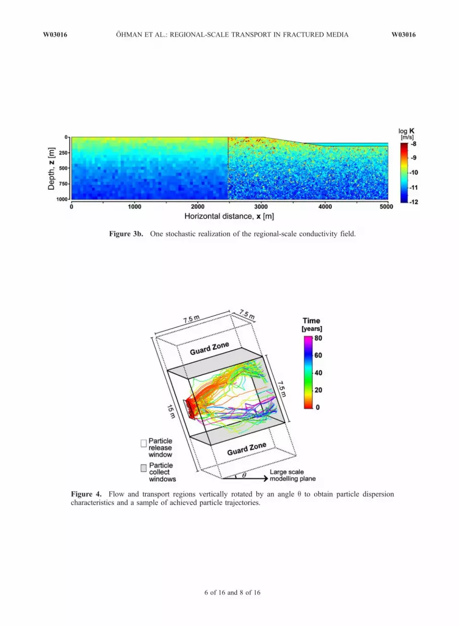
Figure 3b. One stochastic realization of the regional-scale conductivity field.

Figure 4. Flow and transport regions vertically rotated by an angle q to obtain particle dispersioncharacteristics and a sample of achieved particle trajectories.


6 of 16 and 8 of 16

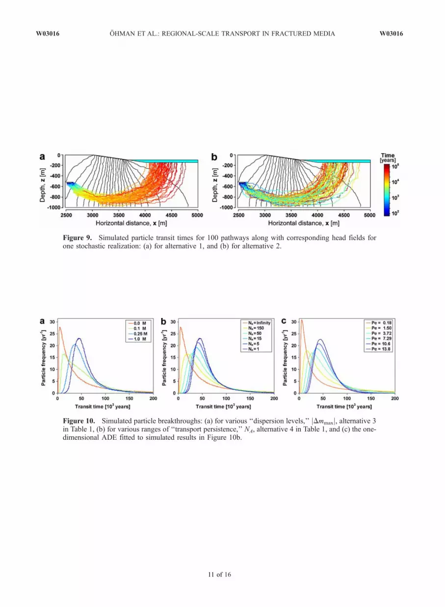
Figure 9. Simulated particle transit times for 100 pathways along with corresponding head fields forone stochastic realization: (a) for alternative 1, and (b) for alternative 2.

Figure 10. Simulated particle breakthroughs: (a) for various ‘‘dispersion levels,’’ jDmmaxj, alternative 3in Table 1, (b) for various ranges of ‘‘transport persistence,’’ NA, alternative 4 in Table 1, and (c) the one-dimensional ADE fitted to simulated results in Figure 10b.


11 of 16

Documents

A regional-scale particle-tracking method for nonstationary fractured media