Iterative image restoration using nonstationary priors

Iterative image restoration using nonstationary priors

Esteban Vera,1,* Miguel Vega,2 Rafael Molina,3 and Aggelos K. Katsaggelos4

1Department of Electrical and Computer Engineering, University of Arizona, Tucson, Arizona 85721, USA2Departamento de Lenguajes y Sistemas Informáticos, Universidad de Granada, Granada 18071, Spain3Departamento de Ciencias de la Computación e I.A., Universidad de Granada, Granada 18071, Spain

4Department of Electrical Engineering and Computer Science, Northwestern University, Evanston, Illinois 60208, USA

*Corresponding author: [email protected]

Received 16 November 2012; revised 11 February 2013; accepted 11 February 2013;posted 12 February 2013 (Doc. ID 179373); published 29 March 2013

In this paper, we propose an algorithm for image restoration based on fusing nonstationary edge-preserving priors. We develop a Bayesian modeling followed by an evidence approximation inferenceapproach for deriving the analytic foundations of the proposed restoration method. Through a seriesof approximations, the final implementation of the proposed image restoration algorithm is iterativeand takes advantage of the Fourier domain. Simulation results over a variety of blurred and noisy stan-dard test images indicate that the presented method comfortably surpasses the current state-of-the-artimage restoration for compactly supported degradations. We finally present experimental results bydigitally refocusing images captured with controlled defocus, successfully confirming the ability ofthe proposed restoration algorithm in recovering extra features and rich details, while still preservingedges. © 2013 Optical Society of AmericaOCIS codes: 100.3020, 100.1830, 100.3190, 110.3010.

1. Introduction

Imaging systems are often affected by several degra-dation sources, leading to blurry and noisy imagesthat are not necessarily a faithful representationof the desired targets. Therefore, and regardless ofthe employed modality, image restoration is a criticaltask for recovering useful imagery for a variety ofapplications, for example, remote sensing, surveil-lance, medical diagnosis, and astronomy [1]. Forinstance, optical imaging systems, such as digitalphotographic or scientific cameras, are not exemptfrom producing degraded imagery, despite the avail-ability of modern CCD or CMOS imaging detectorswith improved resolution, extended dynamic range,and increased quantum efficiency. In digital images,blurring-like degradations can be produced byoptical aberrations or misalignments (optical blur),turbulence (atmospheric blur), or motion due to the

nonzero aperture time (motion blur) [2]. In addition,noise can appear due to quantum and thermal ef-fects, detector nonuniformity, aliasing, electronicsreadout, and quantization.

Unfortunately, the restoration of blurred and noisyimages is an ill-posed inverse problem [3]. Hence-forth, it has to be typically solved by constrained op-timization yielding iterative regularization methods[4]. Nonetheless, regularized image restoration hasto solve two main problems: the choice of the regu-larization function and the regularization parameter,or Lagrange multiplier. The use of Bayesian methodsfor image restoration has emerged as an elegant wayof describing the regularization term by means of aprior distribution, with the additional ability ofallowing estimation of both the regularization andnoise variance weights. Although it has been success-fully applied to smoothness promoting priors [5,6],Bayesianmodeling imposes restrictions on the choiceof the prior function, since some arbitrary priors maylead to intractable inference problems. Nevertheless,the variational Bayes approximation [7] has allowed

1559-128X/13/10D102-09$15.00/0© 2013 Optical Society of America

D102 APPLIED OPTICS / Vol. 52, No. 10 / 1 April 2013

successful use of nonstationary sparsity promotingpriors within the Bayesian framework, such as totalvariation (TV) in [8], Gaussian scale mixtures in [9],and the product of student-t experts in [10,11].

In this paper we propose a new approach to thecombination of nonstationary edge-preserving imagepriors. The novel approach follows the spirit of theprior model based on the product experts first pro-posed in [12], but this time without the need formodifying the observation model, or the need forusing or setting any weighting parameters. Theinference procedure is now based on the evidenceapproximation, or type-II maximum likelihood, con-tinuing the same avenue introduced in [5] for station-ary Bayesian image restoration. However, in thisparticular case, the resulting iterative parameter es-timation update algorithm is computationally intrac-table. Consequently, we propose a series of empiricalapproximations. In this way, the resulting iterativerestoration algorithm is not only effective, but alsoefficient, as it can also be implemented in the Fourierdomain.

We provide simulations for testing the proposedrestoration algorithm and compare its performancewith state-of-the-art Bayesian restoration algorithms.We also present results from a digital refocusingexperiment for images captured with different out-of-focus levels. Quantitative and qualitative evalu-ation of both simulated and real experimental resultsconfirms the extended capabilities of the proposedrestoration method in recovering more appealingimages with enhanced details.

The paper is organized as follows. Section 2presents the Bayes modeling and introduces the pro-posed new prior for the image restoration problem.In Section 3, the inference procedure for image andparameter estimation is derived. Empirical approx-imations are explained in Section 4, leading to anefficient implementation. Sections 5 and 6 presentthe results obtained for the simulations and the dig-ital refocusing experiment. Finally, conclusions aredrawn in Section 7.

2. Bayesian Modeling

A. Observation Model

A typical linear model for image degradation con-siders that the observed image y, in lexicographicalorder, is the result of the convolution of the originaland unknown image x with a blurring kernel opera-tor H plus some additive noise n; that is,

y � Hx� n: (1)

Assuming the noise component n follows aGaussian distribution, the probability density func-tion of the observation model is expressed as

p�yjx; β� ∝ βN∕2 exp�−

β

2‖y −Hx‖2

�; (2)

with β the inverse of the noise variance, and N thetotal number of pixels in the image.

B. Prior Model

Inspired by the results obtained when combiningmore than one single prior, as in the Markov randomfields (MRF) experts used for image denoising in [13],or the sparse prior approach used for image deconvo-lution in [14] and the references therein, we continuedown the path of the product of experts used in [12],but now following a different inference procedurewithout approximating the covariance matrix forthe prior prematurely.

Therefore, as an image prior we define a zero-meanmultivariate Gaussian distribution that combinesthe constraints given by a set of L filtersCi as follows:

p�xja1;…;aL�∝��XLi�1

CtiAiCi

��1∕2

exp�−

12

XLi�1

‖A1∕2i Cix‖

2�;

(3)

where Ai is an N ×N diagonal matrix containing thehyperparameters aj

i associated with the inverse vari-ance (precision) of the response of each correspond-ing filter operator Ci for any given pixel j. Thus,Ai � DIAG�ai�, and ai � �a1

i ; a2i ;…; aN

i �t.The advantage of using the proposed prior model-

ing is twofold. First, we avoid the election of anyspecific sparsity promoting shape for the prior distri-bution, as is done in [10]. Second, by choosing amultivariate Gaussian distribution, we are able toseek a tractable inference mechanism.

3. Bayesian Inference

The joint probability density function is written as

p�y; x; β; a1;…; aL� ∝ p�yjx; β�p�xja1;…; aL�

∝��XLi�1

CtiAiCi

��1∕2

βN∕2

× exp�−

12

XLi�1

‖A1∕2i Cix‖

2�

× exp�−

β

2‖y −Hx‖2

�: (4)

We choose to perform the inference for the desiredhyperparameters based on the evidence analysis—also known as empirical Bayes or type-II maximumlikelihood—previously used in image restorationwith stationary priors in [5,6]. Then, by marginal-izing over x we have that

p�yjβ; a1;…; aL� ∝Zxp�y; x; β; a1;…; aL�dx; (5)

and thus

1 April 2013 / Vol. 52, No. 10 / APPLIED OPTICS D103

ln p�yjβ; a1;…; aL; � �12

ln��XLi�1

CtiAiCi

��N2

ln β

−

12

XLi�1

‖A1∕2i Cix̄‖

2

−

β

2‖y −Hx̄‖2

−

12

ln��XLi�1

CtiAiCi � βHtH

��:(6)

Now, by taking the derivative with respect to thehyperparameter aj

i, we have

δ ln p�yjβ;a1;…;aL�δaj

i

�12

�trace

��XLi�1

CtiAiCi

�−1

CtiJ

jjCi

�

− x̄tCtiJ

jjCix̄−trace��XL

i�1

CtiAiCi�βHtH

�−1

CtiJ

jjCi

��;

(7)

where x̄ is the maximum a posteriori estimate for theunknown image obtained by solving

x̄ ��XL

i�1

CtiAiCi � βHtH

�−1

Hty; (8)

and Jjj is a special selection matrix that is zero every-where except for the entry � jj�. Note that Eq. (8) canbe iteratively solved using a conjugate gradient (CG)minimization algorithm.

Now, by setting the derivative in Eq. (7) equalto zero, and defining ΣP � PL

i�1 CtiAiCi, ΣT �PL

i�1 CtiAiCi � βHtH, and νi � Cix̄, Eq. (7) can be

rewritten as

trace�Σ−1P Ct

iJjjCi� � �νji�2 � trace

�Σ−1T Ct

iJjjCi

: (9)

Then, following a similar approach for updating thehyperparameters to the one in [5], we derived thefollowing iterative formula for any of the hyperpara-meters aj

i at iteration �k� 1�:

aj�k�1�i � trace�Σ�k�−1

P CtiJ

jjCi��ν j�k�

i �2 � trace�Σ�k�−1T Ct

iJjjCi�

aj�k�i ; (10)

where x̄�k� (needed to calculate ν�k�i ) is computed ateach iteration �k� using Eq. (8) with the requiredhyperparameter matrices A�k�

i obtained from theprevious iteration of Eq. (10), along with the corre-sponding covariances Σ�k�−1

P and Σ�k�−1T .

4. Implementation

Unfortunately, the parameter-update formula inEq. (10) is not tractable as is, mostly due to the com-putation of the inverse of the covariance matrices, Σ−1

Pand Σ−1

T , since they are extremely large. Therefore, westart tackling this problem by applying the Jacobidiagonal approximation to the covariance matrices,which leads to the straightforward inversion

Σ�k�−1P ≈ DIAG�ζ�k�P �; Σ�k�−1

T ≈ DIAG�ζ�k�T �: (11)

Here, ζ�k�P and ζ�k�T are N × 1 vectors with componentsζl�k�P � 1∕σl�k�P and ζl�k�T � 1∕σl�k�T , respectively, forl � 1;…; N. Moreover, σ�k�P � P

Li�1 Dia

�k�i and σ�k�T �

σ�k�P � βh2, where Di are N ×N filter matrices withelementsDj

i � �Cji�2, for i � 1;…; L. Also, the constant

h is obtained as the sum of the squares of the pointspread function (PSF) kernel elements, which in thecase of the boxcar (uniform) PSF is equivalent to thevalue of any of the nonzero kernel coefficients.

Using a similar approach, we have

CtiJ

jjCi ≈ Sjji ; (12)

where S jji � DIAG�γ j

i�. Here γ ji � Fij j are N × 1 vec-

tors for i � 1;…; L, while j j is an N × 1 vector thatis zero everywhere except at the position j. Similarlyto the matrices Di, Fi are also N ×N filter matriceswith elements F j

i � �Cji�2. Thus, we finally have that

trace�Σ−1P Ct

iJjjCi� ≈ trace�Σ−1

P Sjji �: (13)

Finally, by applying both approximations providedby Eqs. (11) and (13) over Eq. (10), in addition tostacking into vector form for the different aj�k�1�

icomponents, a new update rule can be obtained foreach of the hyperparameter diagonal matrices asfollows:

A�k�1�i

≈hDIAG

μ�k�i � FiΣ

�k�−1T 1⃗

�i−1DIAG

FiΣ

�k�−1P a�k�i

�;

(14)

where μ�k�i � �ν�k�i �2, and, as explained before, each Fiis related to each respective filter Ci, for j � 1;…; N.

Through experimentation we have found that bet-ter and more stable results are finally obtained whenthe filters Fi are replaced by a unique filter F, whosecorresponding kernel f is given by

f �24 0 1 01 1 10 1 0

35: (15)

Due to the fact that Eq. (14) deals with diagonalmatrices, it can be efficiently implemented in the


Fourier domain. In this way, we have the advantageof obtaining all the diagonal elements of the inverseof each covariance matrix at once, leading to computethe different hyperparameters aj

i in parallel,for i � 1;…; L.

5. Simulation Results

We performed several experiments for restoringimages with simulated blur and noise, using Matlabimplementations of state-of-the-art restoration algo-rithms, and different versions of the herein-proposedrestoration method. We implemented our algorithmin Eq. (14) using two options: NF2 that uses only thefirst-order difference filters, such as

c1 � 1��2

p �1 − 1�; c2 � 1��2

p �1 − 1�t; (16)

and NF4 that also adds the diagonal filters c3 and c4defined as follows:

c3 � 1��2

p�1 00 −1

�; c4 � 1��

2p

�0 1−1 0

�: (17)

We compared the restoration performance of bothversions against implementations of the Bayesian to-tal variation (BTV) approach [8], and the product ofstudent-t priors (BST) [10]. We tested the restorationalgorithms in a set of four standard images: camera-man (CAM, 256 × 256), Lena (LEN, 256 × 256),Shepp–Logan phantom (PHA, 256 × 256) andBarbara (BAR, 512 × 512. The images were degradedby applying one of the following PSFs: a 9 × 9 uni-form blur, or a Gaussian blur with variance σ2 � 9.Also, Gaussian noise was added for achieving anequivalent blurred signal-to-noise ratio (BSNR) of40, 30, or 20 dB.

For all experiments, every algorithm received as in-puts the blurred image, the blurring PSF kernel, andthe noise variance σ2 � 1∕β. In addition, the stoppingcriterion for the iterative update of the hyperpara-meters was that the condition ‖x�k� − x�k−1�‖ < 10−3

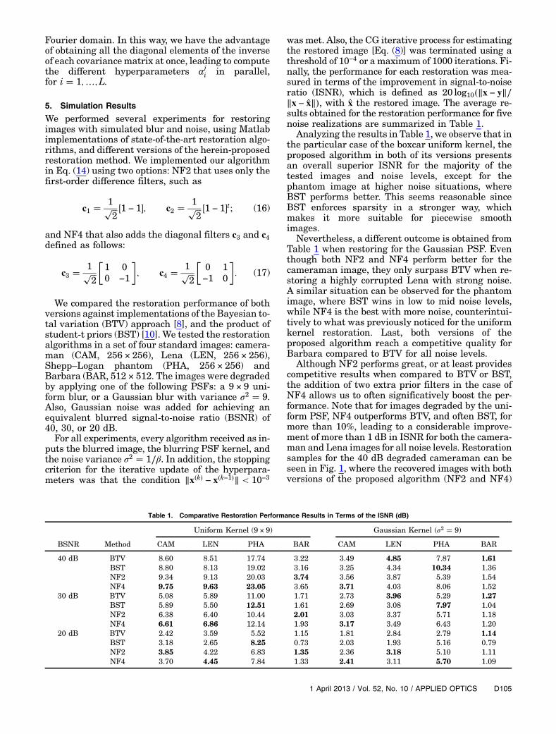
wasmet. Also, the CG iterative process for estimatingthe restored image [Eq. (8)] was terminated using athreshold of 10−4 or a maximum of 1000 iterations. Fi-nally, the performance for each restoration was mea-sured in terms of the improvement in signal-to-noiseratio (ISNR), which is defined as 20 log10�‖x − y‖∕‖x − x̂‖�, with x̂ the restored image. The average re-sults obtained for the restoration performance for fivenoise realizations are summarized in Table 1.

Analyzing the results in Table 1, we observe that inthe particular case of the boxcar uniform kernel, theproposed algorithm in both of its versions presentsan overall superior ISNR for the majority of thetested images and noise levels, except for thephantom image at higher noise situations, whereBST performs better. This seems reasonable sinceBST enforces sparsity in a stronger way, whichmakes it more suitable for piecewise smoothimages.

Nevertheless, a different outcome is obtained fromTable 1 when restoring for the Gaussian PSF. Eventhough both NF2 and NF4 perform better for thecameraman image, they only surpass BTV when re-storing a highly corrupted Lena with strong noise.A similar situation can be observed for the phantomimage, where BST wins in low to mid noise levels,while NF4 is the best with more noise, counterintui-tively to what was previously noticed for the uniformkernel restoration. Last, both versions of theproposed algorithm reach a competitive quality forBarbara compared to BTV for all noise levels.

Although NF2 performs great, or at least providescompetitive results when compared to BTV or BST,the addition of two extra prior filters in the case ofNF4 allows us to often significatively boost the per-formance. Note that for images degraded by the uni-form PSF, NF4 outperforms BTV, and often BST, formore than 10%, leading to a considerable improve-ment of more than 1 dB in ISNR for both the camera-man and Lena images for all noise levels. Restorationsamples for the 40 dB degraded cameraman can beseen in Fig. 1, where the recovered images with bothversions of the proposed algorithm (NF2 and NF4)

Table 1. Comparative Restoration Performance Results in Terms of the ISNR (dB)

Uniform Kernel (9 × 9) Gaussian Kernel (σ2 � 9)

BSNR Method CAM LEN PHA BAR CAM LEN PHA BAR

40 dB BTV 8.60 8.51 17.74 3.22 3.49 4.85 7.87 1.61BST 8.80 8.13 19.02 3.16 3.25 4.34 10.34 1.36NF2 9.34 9.13 20.03 3.74 3.56 3.87 5.39 1.54NF4 9.75 9.63 23.05 3.65 3.71 4.03 8.06 1.52

30 dB BTV 5.08 5.89 11.00 1.71 2.73 3.96 5.29 1.27BST 5.89 5.50 12.51 1.61 2.69 3.08 7.97 1.04NF2 6.38 6.40 10.44 2.01 3.03 3.37 5.71 1.18NF4 6.61 6.86 12.14 1.93 3.17 3.49 6.43 1.20

20 dB BTV 2.42 3.59 5.52 1.15 1.81 2.84 2.79 1.14BST 3.18 2.65 8.25 0.73 2.03 1.93 5.16 0.79NF2 3.85 4.22 6.83 1.35 2.36 3.18 5.10 1.11NF4 3.70 4.45 7.84 1.33 2.41 3.11 5.70 1.09


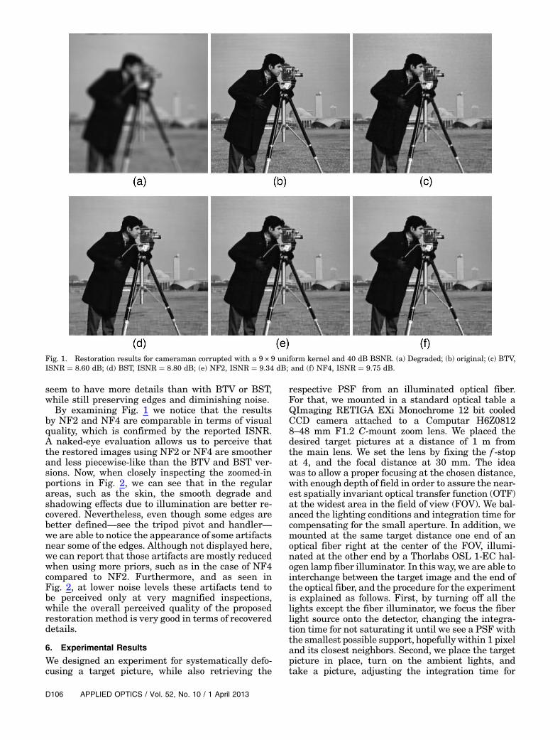
seem to have more details than with BTV or BST,while still preserving edges and diminishing noise.

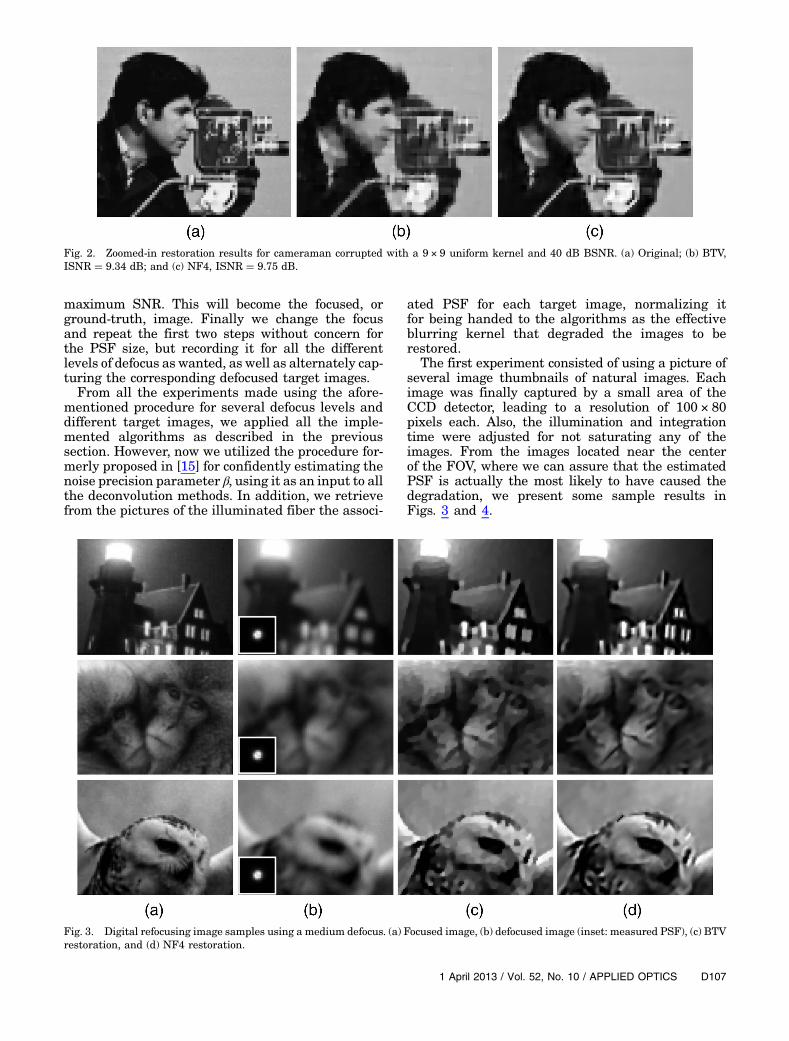
By examining Fig. 1 we notice that the resultsby NF2 and NF4 are comparable in terms of visualquality, which is confirmed by the reported ISNR.A naked-eye evaluation allows us to perceive thatthe restored images using NF2 or NF4 are smootherand less piecewise-like than the BTV and BST ver-sions. Now, when closely inspecting the zoomed-inportions in Fig. 2, we can see that in the regularareas, such as the skin, the smooth degrade andshadowing effects due to illumination are better re-covered. Nevertheless, even though some edges arebetter defined—see the tripod pivot and handler—we are able to notice the appearance of some artifactsnear some of the edges. Although not displayed here,we can report that those artifacts are mostly reducedwhen using more priors, such as in the case of NF4compared to NF2. Furthermore, and as seen inFig. 2, at lower noise levels these artifacts tend tobe perceived only at very magnified inspections,while the overall perceived quality of the proposedrestoration method is very good in terms of recovereddetails.

6. Experimental Results

We designed an experiment for systematically defo-cusing a target picture, while also retrieving the

respective PSF from an illuminated optical fiber.For that, we mounted in a standard optical table aQImaging RETIGA EXi Monochrome 12 bit cooledCCD camera attached to a Computar H6Z08128–48 mm F1.2 C-mount zoom lens. We placed thedesired target pictures at a distance of 1 m fromthe main lens. We set the lens by fixing the f -stopat 4, and the focal distance at 30 mm. The ideawas to allow a proper focusing at the chosen distance,with enough depth of field in order to assure the near-est spatially invariant optical transfer function (OTF)at the widest area in the field of view (FOV). We bal-anced the lighting conditions and integration time forcompensating for the small aperture. In addition, wemounted at the same target distance one end of anoptical fiber right at the center of the FOV, illumi-nated at the other end by a Thorlabs OSL 1-EC hal-ogen lamp fiber illuminator. In this way, we are able tointerchange between the target image and the end ofthe optical fiber, and the procedure for the experimentis explained as follows. First, by turning off all thelights except the fiber illuminator, we focus the fiberlight source onto the detector, changing the integra-tion time for not saturating it until we see a PSF withthe smallest possible support, hopefully within 1 pixeland its closest neighbors. Second, we place the targetpicture in place, turn on the ambient lights, andtake a picture, adjusting the integration time for

Fig. 1. Restoration results for cameraman corrupted with a 9 × 9 uniform kernel and 40 dB BSNR. (a) Degraded; (b) original; (c) BTV,ISNR � 8.60 dB; (d) BST, ISNR � 8.80 dB; (e) NF2, ISNR � 9.34 dB; and (f) NF4, ISNR � 9.75 dB.


maximum SNR. This will become the focused, orground-truth, image. Finally we change the focusand repeat the first two steps without concern forthe PSF size, but recording it for all the differentlevels of defocus as wanted, as well as alternately cap-turing the corresponding defocused target images.

From all the experiments made using the afore-mentioned procedure for several defocus levels anddifferent target images, we applied all the imple-mented algorithms as described in the previoussection. However, now we utilized the procedure for-merly proposed in [15] for confidently estimating thenoise precision parameter β, using it as an input to allthe deconvolution methods. In addition, we retrievefrom the pictures of the illuminated fiber the associ-

ated PSF for each target image, normalizing itfor being handed to the algorithms as the effectiveblurring kernel that degraded the images to berestored.

The first experiment consisted of using a picture ofseveral image thumbnails of natural images. Eachimage was finally captured by a small area of theCCD detector, leading to a resolution of 100 × 80pixels each. Also, the illumination and integrationtime were adjusted for not saturating any of theimages. From the images located near the centerof the FOV, where we can assure that the estimatedPSF is actually the most likely to have caused thedegradation, we present some sample results inFigs. 3 and 4.

Fig. 2. Zoomed-in restoration results for cameraman corrupted with a 9 × 9 uniform kernel and 40 dB BSNR. (a) Original; (b) BTV,ISNR � 9.34 dB; and (c) NF4, ISNR � 9.75 dB.

Fig. 3. Digital refocusing image samples using a medium defocus. (a) Focused image, (b) defocused image (inset: measured PSF), (c) BTVrestoration, and (d) NF4 restoration.


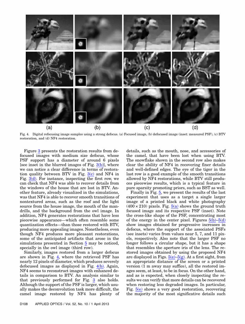
Figure 3 presents the restoration results from de-focused images with medium size defocus, whosePSF support has a diameter of around 6 pixels[see inset in the blurred images of Fig. 3(b)], wherewe can notice a clear difference in terms of restora-tion quality between BTV in Fig. 3(c) and NF4 inFig. 3(d). For instance, inspecting the first row, wecan check that NF4 was able to recover details fromthe windows of the house that are lost in BTV. An-other feature, already visualized in the simulations,was that NF4 is able to recover smooth transitions ofnontextured areas, such as the roof and the lightsource from the house image, the mouth of the man-drills, and the background from the owl image. Inaddition, NF4 generates restorations that have lesspiecewise appearance—which often resemble somequantization effects—than those restored with BTV,producing more appealing images. Nonetheless, eventhough NF4 produces more pleasant restorations,some of the anticipated artifacts that arose in thesimulations presented in Section 5 may be noticed,specially in the owl image (third row).

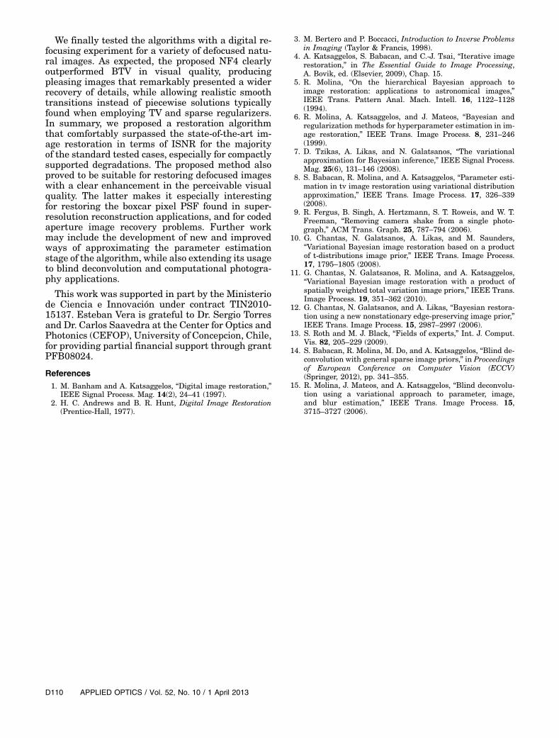
Similarly, images restored from a larger defocusare shown in Fig. 4, where the retrieved PSF hasnearly 12 pixels of diameter, which produces severelydefocused images as displayed in Fig. 4(b). Again,NF4 seems to reconstruct images with enhanced de-tails in comparison to BTV. An analysis similar tothat previously performed for Fig. 3 also holds.Although the support of the PSF is larger, which usu-ally makes the deconvolution task more difficult, thecamel image restored by NF4 has plenty of

details, such as the mouth, nose, and accessories ofthe camel, that have been lost when using BTV.The snowflake shown in the second row also makesclear the ability of NF4 in recovering finer detailsand well-defined edges. The eye of the tiger in thelast row is a good example of the smooth transitionsallowed by NF4 restorations, while BTV still produ-ces piecewise results, which is a typical feature inpure sparsity promoting priors, such as BST as well.

Finally in Fig. 5, we present the results of the lastexperiment that uses as a target a single largerimage of a printed black and white photography(400 × 210) pixels. Fig. 5(a) shows the ground truthfocused image and its respective PSF (inset). Notethe cross-like shape of the PSF, concentrating mostof the energy in the center pixel. Figures 5(b)–5(d)show images obtained for progressive increases indefocus, where the support of the associated PSFs(see insets) varies from values near 5, 7, and 11 pix-els, respectively. Also note that the larger PSF nolonger follows a circular shape, but it has a shapethat resembles the aperture iris of the lens. The re-stored images obtained by using the proposed NF4are displayed in Figs. 5(e)–5(g). At a first sight, froman appropriate distance of the screen or a printedversion (1 m away may suffice), all the restored im-ages seem, at least, to be in focus. On the other hand,and as is expected, when closely inspecting the re-sults we can verify that more details can be recoveredwhen restoring less degraded images. In particular,Fig. 5(e) shows a very good restoration, recoveringthe majority of the most significative details such

Fig. 4. Digital refocusing image samples using a strong defocus. (a) Focused image, (b) defocused image (inset: measured PSF), (c) BTVrestoration, and (d) NF4 restoration.


as the blouse wrinkles and flowers, the hat textures,while wiping out only the finest details of the makeup on the face, when compared to the ground truthimage. Despite performing the restoration of a largerblur see Fig. 5(f) NF4 is still able to recover the mostnoticeable blouse features, and also most of the shad-ows and diffuse reflections on the face. Last, fromFig. 5(g) we can still appreciate most of the importantfeatures of the face, marked by well-defined edgessuch as the nose and eyebrow contour, but most ofthe details have been smeared, which would mostlikely happen as well when using any other edge pre-serving deconvolution algorithm, such as BTV,although not as smoothly as with NF4.

7. Conclusion

In this paper, we proposed a new algorithm for imagerestoration based on combining nonstationary edge-preserving priors. We developed a Bayesian model-ing followed by an evidence analysis inferenceapproach for deriving the initial parameter-updatealgorithm. From there, the iterative algorithm was

empirically approximated tackling its computationaldifficulties, mostly related to the inversion of largeand ill-posed covariance matrices, and also allowinga fast and efficient implementation through theFourier domain. When comparing the restoration re-sults of the proposed method with some of the lateststate-of-the-art image restoration algorithms (BTV[8] and BST [10]) on a set of standard test imageswith simulated blurring and noise, we concluded thatdespite some exceptions, the proposed algorithmoutperformed the current available methods interms of ISNR and visual quality, especially when re-storing natural images from blur kernels withcompact support. The reported ISNR values, inparticular for the uniform PSF, indicate that theproposed algorithm, in all its implemented versions,surpassed by more than 10% the other methods,reaching a gap of more than 1 dB for the classiccameraman and Lena test images for all noise levels.Nevertheless, for the Gaussian PSF case the resultswere not the most prominent ones, but they werecompetitive.

Fig. 5. Digital refocusing experiment. (a) Focused image (inset: 4×measured PSF), (b) moderate defocus image (inset: 4×measured PSF),(c) medium defocus image (inset: 4× measured PSF), (d) strong defocus image (inset: 4× measured PSF), (e) restored image (b) using NF4,(f) restored image (c) using NF4, (g) restored image (d) using NF4.


We finally tested the algorithms with a digital re-focusing experiment for a variety of defocused natu-ral images. As expected, the proposed NF4 clearlyoutperformed BTV in visual quality, producingpleasing images that remarkably presented a widerrecovery of details, while allowing realistic smoothtransitions instead of piecewise solutions typicallyfound when employing TV and sparse regularizers.In summary, we proposed a restoration algorithmthat comfortably surpassed the state-of-the-art im-age restoration in terms of ISNR for the majorityof the standard tested cases, especially for compactlysupported degradations. The proposed method alsoproved to be suitable for restoring defocused imageswith a clear enhancement in the perceivable visualquality. The latter makes it especially interestingfor restoring the boxcar pixel PSF found in super-resolution reconstruction applications, and for codedaperture image recovery problems. Further workmay include the development of new and improvedways of approximating the parameter estimationstage of the algorithm, while also extending its usageto blind deconvolution and computational photogra-phy applications.

This work was supported in part by the Ministeriode Ciencia e Innovación under contract TIN2010-15137. Esteban Vera is grateful to Dr. Sergio Torresand Dr. Carlos Saavedra at the Center for Optics andPhotonics (CEFOP), University of Concepcion, Chile,for providing partial financial support through grantPFB08024.

References1. M. Banham and A. Katsaggelos, “Digital image restoration,”

IEEE Signal Process. Mag. 14(2), 24–41 (1997).2. H. C. Andrews and B. R. Hunt, Digital Image Restoration

(Prentice-Hall, 1977).

3. M. Bertero and P. Boccacci, Introduction to Inverse Problemsin Imaging (Taylor & Francis, 1998).

4. A. Katsaggelos, S. Babacan, and C.-J. Tsai, “Iterative imagerestoration,” in The Essential Guide to Image Processing,A. Bovik, ed. (Elsevier, 2009), Chap. 15.

5. R. Molina, “On the hierarchical Bayesian approach toimage restoration: applications to astronomical images,”IEEE Trans. Pattern Anal. Mach. Intell. 16, 1122–1128(1994).

6. R. Molina, A. Katsaggelos, and J. Mateos, “Bayesian andregularization methods for hyperparameter estimation in im-age restoration,” IEEE Trans. Image Process. 8, 231–246(1999).

7. D. Tzikas, A. Likas, and N. Galatsanos, “The variationalapproximation for Bayesian inference,” IEEE Signal Process.Mag. 25(6), 131–146 (2008).

8. S. Babacan, R. Molina, and A. Katsaggelos, “Parameter esti-mation in tv image restoration using variational distributionapproximation,” IEEE Trans. Image Process. 17, 326–339(2008).

9. R. Fergus, B. Singh, A. Hertzmann, S. T. Roweis, and W. T.Freeman, “Removing camera shake from a single photo-graph,” ACM Trans. Graph. 25, 787–794 (2006).

10. G. Chantas, N. Galatsanos, A. Likas, and M. Saunders,“Variational Bayesian image restoration based on a productof t-distributions image prior,” IEEE Trans. Image Process.17, 1795–1805 (2008).

11. G. Chantas, N. Galatsanos, R. Molina, and A. Katsaggelos,“Variational Bayesian image restoration with a product ofspatially weighted total variation image priors,” IEEE Trans.Image Process. 19, 351–362 (2010).

12. G. Chantas, N. Galatsanos, and A. Likas, “Bayesian restora-tion using a new nonstationary edge-preserving image prior,”IEEE Trans. Image Process. 15, 2987–2997 (2006).

13. S. Roth and M. J. Black, “Fields of experts,” Int. J. Comput.Vis. 82, 205–229 (2009).

14. S. Babacan, R. Molina, M. Do, and A. Katsaggelos, “Blind de-convolution with general sparse image priors,” in Proceedingsof European Conference on Computer Vision (ECCV)(Springer, 2012), pp. 341–355.

15. R. Molina, J. Mateos, and A. Katsaggelos, “Blind deconvolu-tion using a variational approach to parameter, image,and blur estimation,” IEEE Trans. Image Process. 15,3715–3727 (2006).


Documents

Iterative image restoration using nonstationary priors