Online sequential extreme learning machine in nonstationary environments

Online Sequential Extreme Learning Machine inNonstationary Environments

Yibin Ye, Stefano Squartini, Francesco Piazza

A3LAB, Department of Information Engineering,Universita Politecnica delle Marche, Via Brecce Bianche 1, 60131 Ancona, Italy

{ yibin.ye,s.squartini,f.piazza}@univpm.ithttp:// www. a3lab.dibet.univpm.it

Abstract

System Identification in nonstationary environments represents a challengingproblem to solve and lots of e!orts have been put by the scientific communityin the last decades to provide adequate solutions on purpose. Most of themare targeted to work under the system linearity assumption, but also somehave been proposed to deal with the nonlinear case study. In particular theauthors have recently advanced a neural architecture, namely Time-VaryingNeural Networks (TV-NN), which has shown remarkable identification prop-erties in presence of nonlinear and nonstationary conditions. TV-NN trainingis an issue due to the high number of free parameters and the Extreme Learn-ing Machine (ELM) approach has been successfully used on purpose. ELM isa fast learning algorithm that has recently caught much attention within theNeural Networks (NNs) research community. Many variants of ELM havebeen appeared in recent literature, specially for the stationary case study.The reference one for TV-NN training is named ELM-TV and is of batch-learning type. In this contribution an online sequential version of ELM-TV isdeveloped, in response to the need of dealing with applications where sequen-tial arrival or large number of training data occurs. This algorithm general-izes the corresponding counterpart working under stationary conditions. Itsperformances have been evaluated in some nonstationary and nonlinear sys-tem identification tasks and related results show that the advanced techniqueproduces comparable generalization performances to ELM-TV, ensuring atthe same time all benefits of an online sequential approach.

Keywords: Nonstationary and Nonlinear System Identification,Time-Varying Neural Networks, Extreme Learning Machine, Online

Preprint submitted to Neurocomputing November 10, 2011

Sequential Learning

1. Introduction

Extreme Learning Machine (ELM) is a fast learning algorithm designedfor single hidden layer feedforward neural networks (SLFNs) [1], first intro-duced by Huang et al. In ELM, the input weights of SLFNs do not needto be tuned and can be randomly generated, whereas the output weightsare analytically determined using the least-square method, thus allowing asignificant training time reduction. In recent years, ELM has been raisingmuch attention and interest among scientific community, in both theoreticstudy and applications. A hybrid algorithm called Evolutionary ExtremeLearning Machine (E-ELM) [2] uses the di!erential evolutionary algorithmto select the input weights. Incremental-based Extreme Learning Machinealgorithms (I-ELM [3], EI-ELM [4] and EM-ELM [5]) can randomly addnodes to the hidden layer. A real-coded genetic algorithm approach calledRCGA-ELM has been also proposed to select the optimal number of hid-den nodes, input weights and bias values for better performance in multi-category sparse data classification problems [6]. B-ELM is able to optimizethe weights of the output layer based on a Bayesian linear regression [7]. TheOptimally Pruned Extreme Learning Machine (OP-ELM) extends the orig-inal ELM algorithm and wraps it within a methodology using a pruning ofthe neurons [8]. In CFWNN-ELM, Composite Functions are applied at thehidden nodes and learning is accomplished using ELM in a Wavelet NeuralNetwork [9]. Encoding a priori information to obtain better generalizationperformance for function approximation is another possible way to improveELM [10]. Radial-basis type neural networks [11, 12] also represent a fertilefield where ELM paradigm has found application, as confirmed by some re-cent contributions[13, 1]. Aong the various extensions, the online sequentiallearning algorithm based on ELM (OS-ELM) need to be cited, accordingto which learning is performed by using data one-by-one or chunk-by-chunkwith fixed or varying chunk size [14]. The parameters of hidden nodes arerandomly selected just as ELM, but the output weights are analytically up-dated based on the sequentially arriving data rather than the whole dataset. Besides theoretical studies, some applications such as system identifi-cation and real-time data assessment have been considered to evaluate thee!ectiveness of ELM [15, 16].

2

Time-Varying Neural Network (TV-NN) represents a relevant example inneural architectures working properly in nonstationary environments. Suchnetworks implement time-varying weights, each being a linear combinationof a certain set of basis functions, whose independent variable is time. Thecandidate orthogonal basis function types employed in time-varying networksinclude Legendre polynomials, Chebyshev polynomials, Fourier sinusoidalfunctions, Prolate spheroidal functions [17], and more. An extended Back-Propagation algorithm has been first advanced to train these networks (BP-TV) [18]. Later on, an Extreme Learning Machine approach is also developedfor TV-NN, accelerating the training procedure significantly (ELM-TV) [19].Recently, several variants and applications have been proposed based onELM-TV. A group selection evolutionary approach applies di!erential evo-lutionary with group selection to determine the type of basis function andits input weight parameters [20], while two other algorithms referred as EM-ELM-TV [21] and EM-OB [22] are able to automatically determine the num-ber of hidden neurons or output basis functions, respectively. A Volterrasystem identification application is also studied in [23].

All the algorithms for TV-NN mentioned above belong to batch-learningtype. BP-TV is a time consuming algorithm as it involve many epochs (oriterations). Meanwhile, learning parameters such as learning rate, numberof learning epochs have to be properly chosen to ensure convergence. As forELM-based algorithms, whenever a new data arrived, the past data alongwith the new one have to be used for retraining, thus consuming lots oftime or/and memory. With the advantage of no requirement for retrainingwhenever receiving new data, online learning algorithms are preferred overbatch ones in some engineering applications.

Based on [14], in this paper, an online extreme learning machine is ex-tended to deal with time-varying neural networks and referred as OS-ELM-TV, which can learn the training data one-by-one or chunk-by-chunk. Thedata which have already been used in the training can be discarded, so as tosave more memory and computational load to process the new coming data.

The paper is organized as follows. The ELM and ELM-TV algorithmsare briefly introduced in Section 2 and 3, followed by our proposed On-LineELM-TV presented in Section 4 and computational complexity analysis inSection 5. Computer simulations and related results are demonstrated anddiscussed in Section 6. Finally conclusions are drawn in Section 7.

3

2. Extreme Learning Machine

Let’s assume that an SLFN with I input neurons, K hidden neurons, Loutput neurons and activation function g(·) is trained to learn N distinctsamples (X,T), where X = {xi[n]} ! RN!I and T = {tl[n]} ! RN!L are theinput matrix and target matrix respectively, xi[n] denotes the input data ini-th input neuron at n-th time instant, and tl[n] denotes the desired outputin l-th output neuron at n-th time instant. In ELM, the input weights {wik}and hidden biases {bk} are randomly generated, where wik is the weightconnecting i input neuron to k-th hidden neuron, and bk is the bias of k-thhidden neuron. Further let w0k = bk and x0[n] = 1. Hence, the hidden-layeroutput matrix H = {hk[n]} ! RN!K can be obtained by:

hk[n] = g

!I"

i=0

xi[n] · wik

#

(1)

Let ! = {!kl} ! RK!L be the matrix of output weights, where !kl denotesthe weight connection between k-th hidden neuron and l-th output neuron;and Y = {yl[n]} ! RN!L be the matrix of network output data, with yl[n]the output data in l-th output neuron at n-th time instant. Therefore, thisequation can be obtained for the linear output neurons:

yl[n] =K"

k=1

hk[n] · !kl (2)

or Y = H · ! (3)

Thus, given the hidden-layer output matrix H and the targets matrix T,to minimize "Y#T"2, the output weights can be calculated by the minimumnorm least-square(LS) solution of the linear system:

! = H† · T, (4)

where H† is the Moore-Penrose generalized inverse of matrix H. By com-puting output weights analytically, ELM achieve good generalization perfor-mance with speedy training phase.

3. ELM for Time-varying Neural Networks

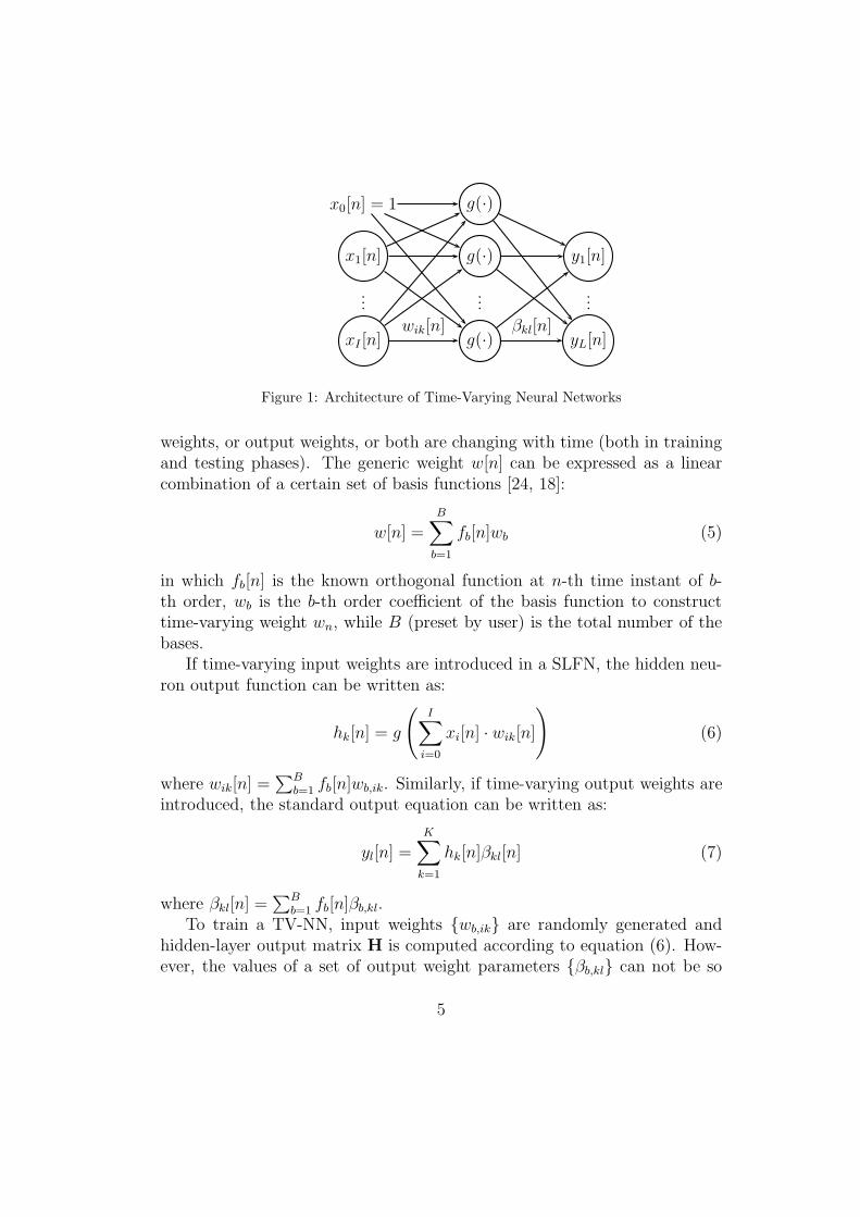
The time-varying version of Extreme Learning Machine has been studiedin [19]. In a time-varying neural network as shown in Fig. 1, the input

4

x0[n] = 1 g(·)

x1[n] g(·) y1[n]

......

...

xI [n] g(·) yL[n]wik[n] !kl[n]

Figure 1: Architecture of Time-Varying Neural Networks

weights, or output weights, or both are changing with time (both in trainingand testing phases). The generic weight w[n] can be expressed as a linearcombination of a certain set of basis functions [24, 18]:

w[n] =B"

b=1

fb[n]wb (5)

in which fb[n] is the known orthogonal function at n-th time instant of b-th order, wb is the b-th order coe"cient of the basis function to constructtime-varying weight wn, while B (preset by user) is the total number of thebases.

If time-varying input weights are introduced in a SLFN, the hidden neu-ron output function can be written as:

hk[n] = g

!I"

i=0

xi[n] · wik[n]

#

(6)

where wik[n] =$B

b=1 fb[n]wb,ik. Similarly, if time-varying output weights areintroduced, the standard output equation can be written as:

yl[n] =K"

k=1

hk[n]!kl[n] (7)

where !kl[n] =$B

b=1 fb[n]!b,kl.To train a TV-NN, input weights {wb,ik} are randomly generated and

hidden-layer output matrix H is computed according to equation (6). How-ever, the values of a set of output weight parameters {!b,kl} can not be so

5

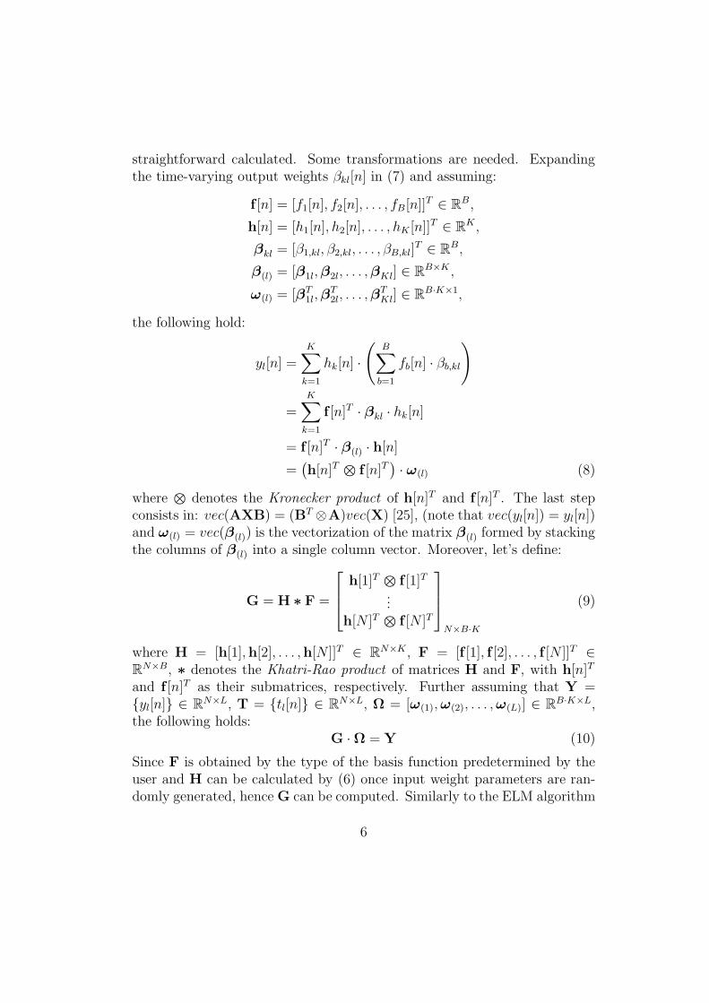
straightforward calculated. Some transformations are needed. Expandingthe time-varying output weights !kl[n] in (7) and assuming:

f [n] = [f1[n], f2[n], . . . , fB[n]]T ! RB,

h[n] = [h1[n], h2[n], . . . , hK [n]]T ! RK ,

!kl = [!1,kl, !2,kl, . . . , !B,kl]T ! RB,

!(l) = [!1l, !2l, . . . , !Kl] ! RB!K ,

"(l) = [!T1l, !

T2l, . . . , !

TKl] ! RB·K!1,

the following hold:

yl[n] =K"

k=1

hk[n] ·!

B"

b=1

fb[n] · !b,kl

#

=K"

k=1

f [n]T · !kl · hk[n]

= f [n]T · !(l) · h[n]

=%h[n]T ! f [n]T

&· "(l) (8)

where ! denotes the Kronecker product of h[n]T and f [n]T . The last stepconsists in: vec(AXB) = (BT $A)vec(X) [25], (note that vec(yl[n]) = yl[n])and "(l) = vec(!(l)) is the vectorization of the matrix !(l) formed by stackingthe columns of !(l) into a single column vector. Moreover, let’s define:

G = H " F =

'

()h[1]T ! f [1]T

...h[N ]T ! f [N ]T

*

+,

N!B·K

(9)

where H = [h[1],h[2], . . . ,h[N ]]T ! RN!K , F = [f [1], f [2], . . . , f [N ]]T !RN!B, " denotes the Khatri-Rao product of matrices H and F, with h[n]T

and f [n]T as their submatrices, respectively. Further assuming that Y ={yl[n]} ! RN!L, T = {tl[n]} ! RN!L, ! = ["(1), "(2), . . . , "(L)] ! RB·K!L,the following holds:

G ·! = Y (10)

Since F is obtained by the type of the basis function predetermined by theuser and H can be calculated by (6) once input weight parameters are ran-domly generated, hence G can be computed. Similarly to the ELM algorithm

6

described in previous section, the time-variant output weight matrix ! canbe computed by:

! = G† · T (11)

where G† is the MP inverse of matrix G, and consequently, ! is a set ofoptimal output weight parameters minimizing the training error.

4. The proposed algorithm: Online Sequential ELM-TV

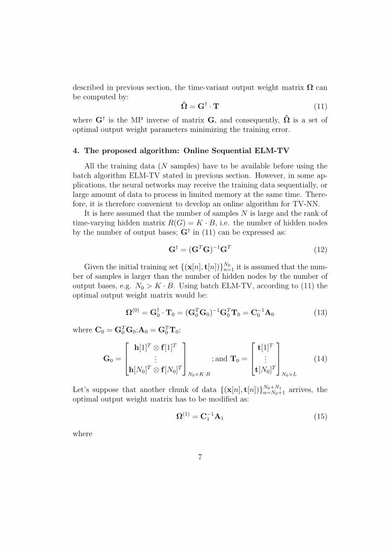
All the training data (N samples) have to be available before using thebatch algorithm ELM-TV stated in previous section. However, in some ap-plications, the neural networks may receive the training data sequentially, orlarge amount of data to process in limited memory at the same time. There-fore, it is therefore convenient to develop an online algorithm for TV-NN.

It is here assumed that the number of samples N is large and the rank oftime-varying hidden matrix R(G) = K · B, i.e. the number of hidden nodesby the number of output bases; G† in (11) can be expressed as:

G† = (GTG)"1GT (12)

Given the initial training set {(x[n], t[n])}N0n=1 it is assumed that the num-

ber of samples is larger than the number of hidden nodes by the number ofoutput bases, e.g. N0 > K ·B. Using batch ELM-TV, according to (11) theoptimal output weight matrix would be:

!(0) = G†0 ·T0 = (GT

0 G0)"1GT

0 T0 = C"10 A0 (13)

where C0 = GT0 G0;A0 = GT

0 T0;

G0 =

'

()h[1]T $ f [1]T

...h[N0]T $ f [N0]T

*

+,

N0!K·B

; and T0 =

'

()t[1]T

...t[N0]T

*

+,

N0!L

(14)

Let’s suppose that another chunk of data {(x[n], t[n])}N0+N1n=N0+1 arrives, the

optimal output weight matrix has to be modified as:

!(1) = C"11 A1 (15)

where

7

C1 =

-G0

G1

.T -G0

G1

.=

/GT

0 GT1

0 -G0

G1

.= C0 + GT

1 G1 (16)

A1 =

-G0

G1

.T -T0

T1

.=

/GT

0 GT1

0 -T0

T1

.= A0 + GT

1 T1 (17)

G1 =

'

()h[N0 + 1]T $ f [N0 + 1]T

...h[N0 + N1]T $ f [N0 + N1]T

*

+,

N1!K·B

;T1 =

'

()t[N0 + 1]T

...t[N0 + N1]T

*

+,

N1!L

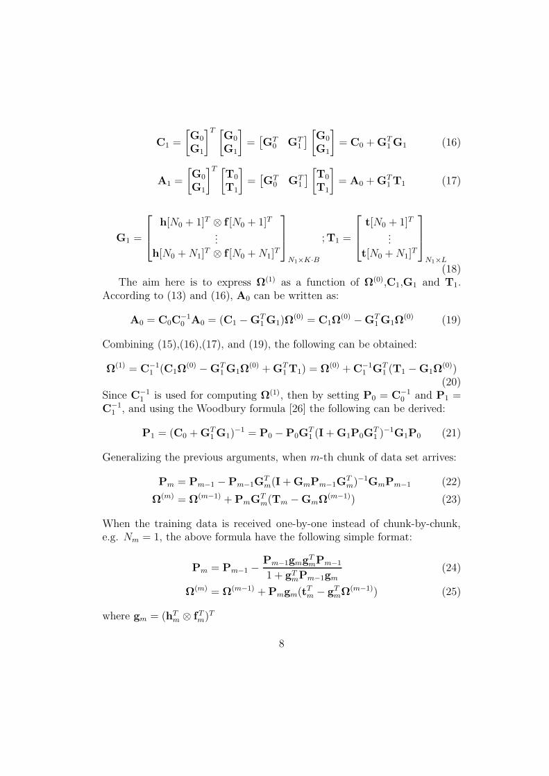
(18)The aim here is to express !(1) as a function of !(0),C1,G1 and T1.

According to (13) and (16), A0 can be written as:

A0 = C0C"10 A0 = (C1 # GT

1 G1)!(0) = C1!

(0) #GT1 G1!

(0) (19)

Combining (15),(16),(17), and (19), the following can be obtained:

!(1) = C"11 (C1!

(0) # GT1 G1!

(0) + GT1 T1) = !(0) + C"1

1 GT1 (T1 #G1!

(0))(20)

Since C"11 is used for computing !(1), then by setting P0 = C"1

0 and P1 =C"1

1 , and using the Woodbury formula [26] the following can be derived:

P1 = (C0 + GT1 G1)

"1 = P0 # P0GT1 (I + G1P0G

T1 )"1G1P0 (21)

Generalizing the previous arguments, when m-th chunk of data set arrives:

Pm = Pm"1 # Pm"1GTm(I + GmPm"1G

Tm)"1GmPm"1 (22)

!(m) = !(m"1) + PmGTm(Tm #Gm!

(m"1)) (23)

When the training data is received one-by-one instead of chunk-by-chunk,e.g. Nm = 1, the above formula have the following simple format:

Pm = Pm"1 #Pm"1gmgT

mPm"1

1 + gTmPm"1gm

(24)

!(m) = !(m"1) + Pmgm(tTm # gT

m!(m"1)) (25)

where gm = (hTm $ fT

m)T

8

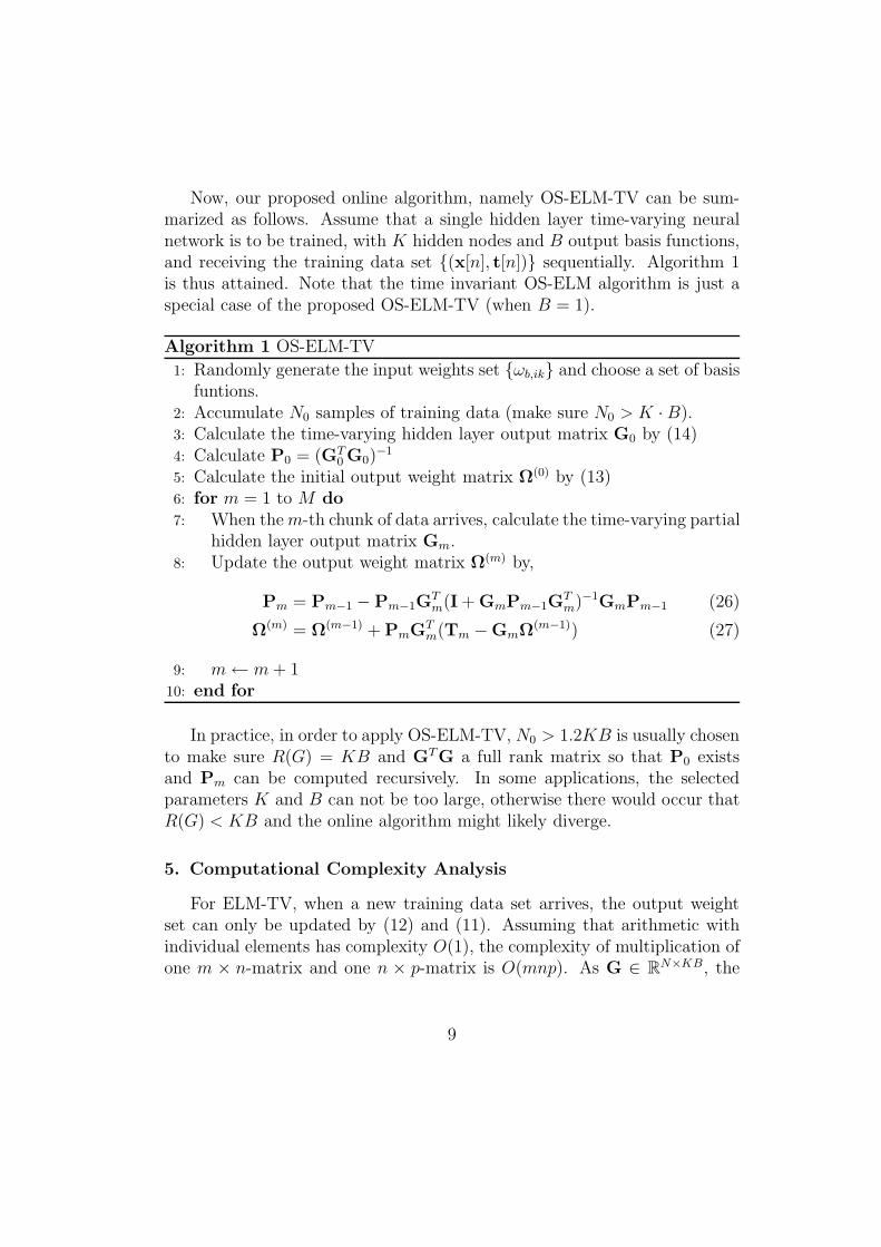
Now, our proposed online algorithm, namely OS-ELM-TV can be sum-marized as follows. Assume that a single hidden layer time-varying neuralnetwork is to be trained, with K hidden nodes and B output basis functions,and receiving the training data set {(x[n], t[n])} sequentially. Algorithm 1is thus attained. Note that the time invariant OS-ELM algorithm is just aspecial case of the proposed OS-ELM-TV (when B = 1).

Algorithm 1 OS-ELM-TV1: Randomly generate the input weights set {"b,ik} and choose a set of basis

funtions.2: Accumulate N0 samples of training data (make sure N0 > K · B).3: Calculate the time-varying hidden layer output matrix G0 by (14)4: Calculate P0 = (GT

0 G0)"1

5: Calculate the initial output weight matrix !(0) by (13)6: for m = 1 to M do7: When the m-th chunk of data arrives, calculate the time-varying partial

hidden layer output matrix Gm.8: Update the output weight matrix !(m) by,

Pm = Pm"1 # Pm"1GTm(I + GmPm"1G

Tm)"1GmPm"1 (26)

!(m) = !(m"1) + PmGTm(Tm #Gm!

(m"1)) (27)

9: m % m + 110: end for

In practice, in order to apply OS-ELM-TV, N0 > 1.2KB is usually chosento make sure R(G) = KB and GTG a full rank matrix so that P0 existsand Pm can be computed recursively. In some applications, the selectedparameters K and B can not be too large, otherwise there would occur thatR(G) < KB and the online algorithm might likely diverge.

5. Computational Complexity Analysis

For ELM-TV, when a new training data set arrives, the output weightset can only be updated by (12) and (11). Assuming that arithmetic withindividual elements has complexity O(1), the complexity of multiplication ofone m & n-matrix and one n & p-matrix is O(mnp). As G ! RN!KB, the

9

computational complexities of two matrix multiplications and one matrixinversion in G† = (GTG)"1GT are O((KB)2N) and O((KB)3) respectively.

For calculation of output weight matrix ! = G† · T, with G† ! RKB!N

and T ! RN!L, the computational complexity of (11) is O((KB)NL).Since KB < N and usually L < KB, it can be concluded that the

computational complexity of updating ! is O((KB)2N).On the other hand, for online ELM-TV, when m-th chunk of data set

arrives, (22) and (23) are used to update the output weight set. As Pm"1 !RKB!KB and Gm ! RNm!KB, the computational complexity required tocalculate Pm in (22) is O((KB)2Nm).

Similarly, as !(m"1) ! RKB!L and the common case of L < KB, the com-putational complexity to obtain !(m) from (23) would also be O((KB)2Nm).Since usually Nm ' N , the computational complexity (in terms of compu-tational load and memory comsumption) when applying the proposed OS-ELM-TV rather than the standard ELM-TV, would be reduced dramaticallyfor updating output weight matrix. This is especially true for the case of largetotal samples (N > 103) with one-by-one data set arrival (Nm = 1).

As for memory requirements, intuitively one can expect that OS-ELM-TVuses less memory since previous samples can be discarded after the updatingprocess. In fact, in ELM-TV, G ! RN!KB and T ! RN!L have to be alwaysstored; moreover the memory required for computation of G† increases whenN becomes larger. On the other hand, in the OS-ELM-TV algorithm, wehave that only the variable Pm ! RKB!KB rather than G and T needs tobe stored and that calculations of smaller matrices w.r.t. the ELM-TV casestudy are involved in the weights updating process.

6. Computer Simulations

In this section, OS-ELM-TV (in one-by-one learning mode) is comparedwith ELM-TV in three identification problems and one estimation task,which can all be categorized as time-varying system identification problemsand represent a certain range of nonstationary environment. The polynomialactivation function (g(x) = x2 + x) is used in TV-NN networks. All simula-tions have been accomplished by means of the MATLAB 7.8.0 programmingenvironment, running on an Intel Core2 Duo CPU P8400 2.26GHz, withWindows Vista OS.

10

Basis Function Algorithms Training Validation Training(#input, #output) RMSE(dB) RMSE(dB) Time (s)

None(1,1)ELM -19.26 -18.86 0.0409

OS-ELM -19.25 -18.84 0.0046

Legendre(3,1)ELM-TV -19.45 -18.96 0.0449

OS-ELM-TV -19.13 -18.79 0.0057

Legendre(1,3)ELM-TV -26.98 -22.25 0.2350

OS-ELM-TV -26.98 -22.19 0.0092

Legendre(3,3)ELM-TV -32.24 -25.57 0.2898

OS-ELM-TV -33.68 -26.55 0.0071

Chebyshev(3,3)ELM-TV -32.77 -26.47 0.3729

OS-ELM-TV -33.28 -26.07 0.0095

Prolate(3,3)ELM-TV -33.90 -29.79 0.2774

OS-ELM-TV -32.61 -29.21 0.0077

Fourier(3,3)ELM-TV -20.32 -18.44 0.2883

OS-ELM-TV -20.50 -18.48 0.0085

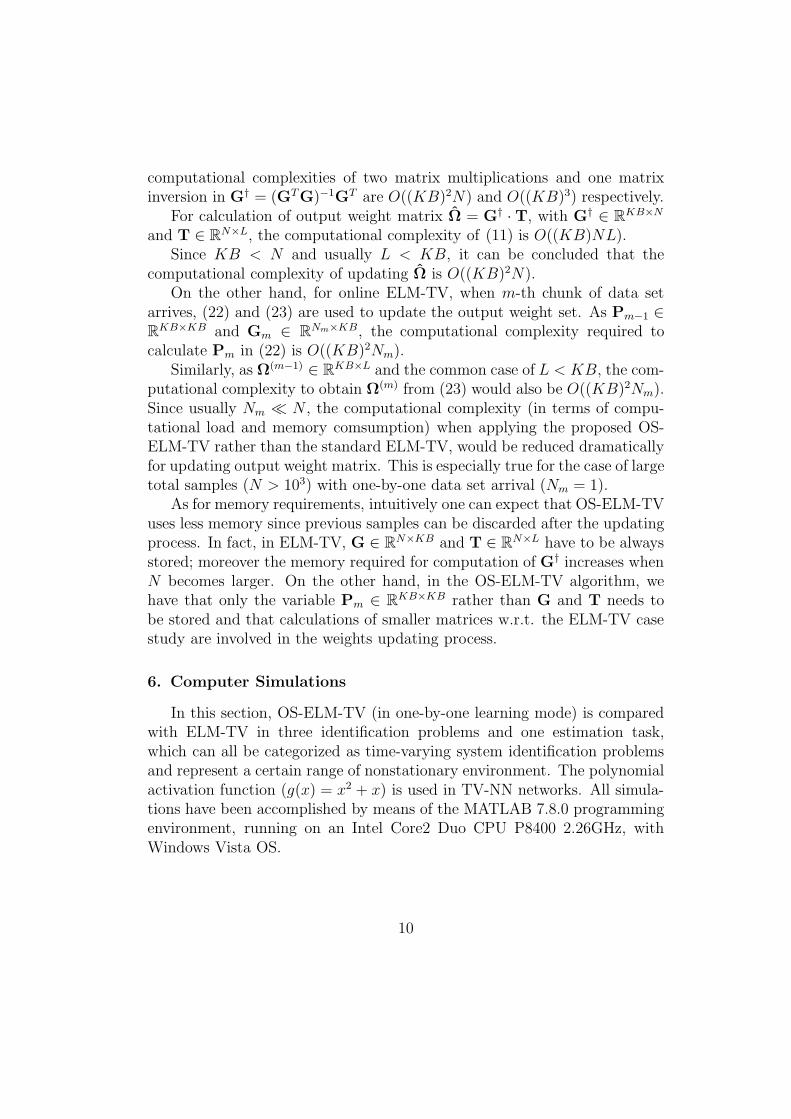
Table 1: Performance Comparisons of ELM-TV and OS-ELM-TV with di!erent basisfunctions and number of input/output bases when updating the 1000th sample in time-varying MLP system, with 100 hidden nodes

6.1. Time-varying MLP system identification

The system to be identified here is the same to that in [18] and [19]: atime-varying IIR-bu!ered MLP with 11 input lines, one 5 neurons hiddenlayer, one neuron output layer. The input weights and output weights arecombinations of 3 Prolate basis functions; the length of the input and outputTime Delay Lines (TDLs) is equal to 6 and 5 respectively. Note that theoutput neuron of this system is not linear, both the hidden neurons andoutput neuron use tangent sigmoid activation function.

6.2. Time-varying Narendra system identification

The next test identification system is a modified version of the one ad-dressed in [27], by adding the coe"cients a[n] and b[n], which are low passfiltered versions of a random sequence, to form a time-varying system, as

11

400 500 600 700 800 900 10000

0.05

0.1

0.15

0.2

0.25

0.3

0.35Training Time of MLP System

Training Samples

Trai

ning

Tim

e(s)

OS ELM TVELM TV

400 500 600 700 800 900 100045

40

35

30

25

20

15

10

5

0

5

Training SamplesRM

SE(d

B)

Generalization Performance of MLP System

OS ELM TV TrainingOS ELM TV ValidationELM TV TrainingELM TV Validation

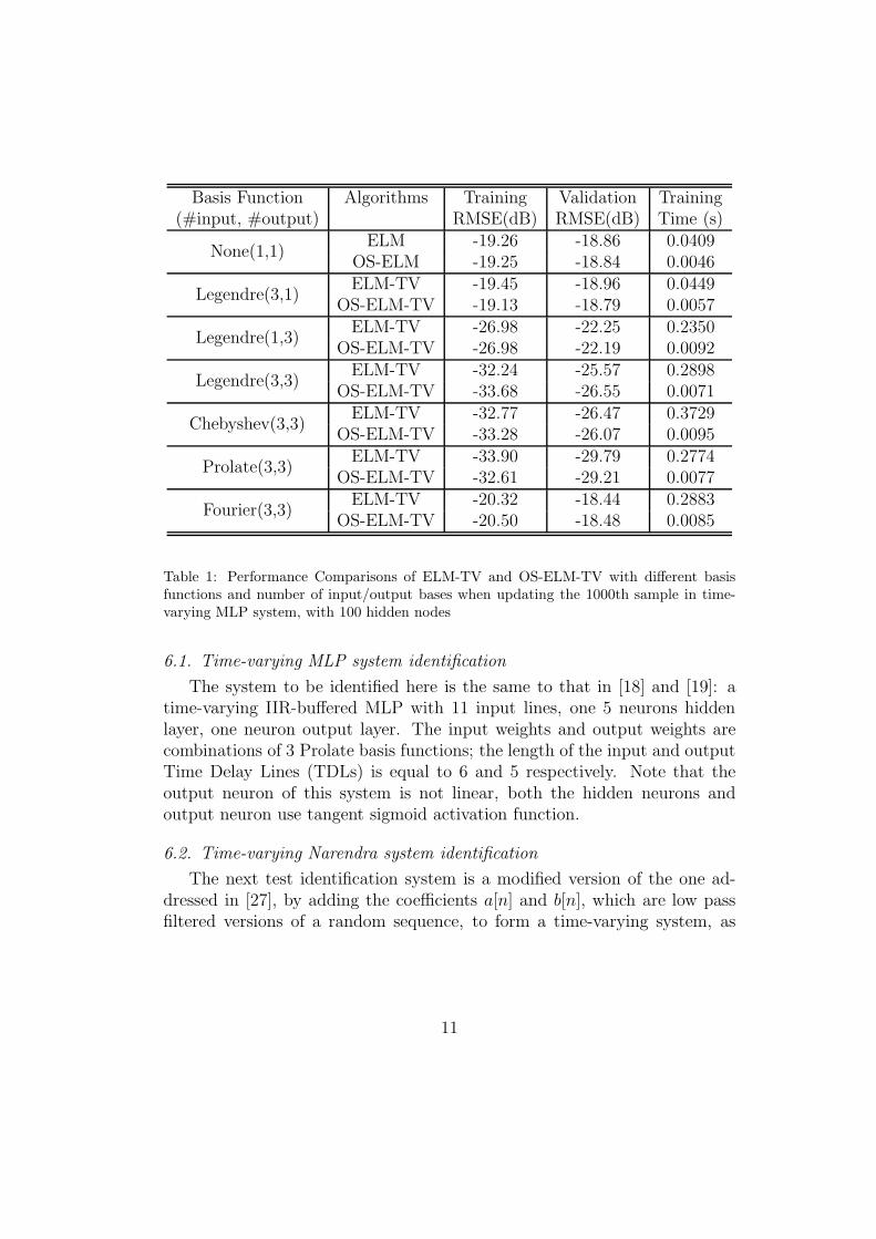
Figure 2: Performance Comparisons of ELM-TV and OS-ELM-TV for MLP system withparameter settings as: Legendre basis functions, 3 input bases, 3 output bases and 100hidden nodes

done in [18] and [19]:

y[n] = a[n] · y[n # 1] · y[n # 2] · y[n # 3] · x[n # 1] · (y[n # 3] # 1) + x[n]

1 + b[n] · (y[n # 3]2 + y[n # 2]2)(28)

The model used for this identification task is a time-varying IIR-bu!eredneural network with 5 input lines, where 3 of them are produced by the inputTDL and the remaining 2 by the output feedback TDL.

6.3. Time-varying Volterra system identification

Volterra models are widely used to represent nonlinear systems due tothe Weierstrass approximation theorem, which states that every continuousfunction defined on a finite closed interval can be uniformly approximated asclosely as desired by a polynomial function. On the one hand, Volterra sys-tem is usually assumed to be time-invariant in most reported Volterra systemrelated literature [28, 29]. On the other hand, time variation characteristicshas to be considered in many real applications such as communication chan-nels modelling, speech processing, and biological systems. In these cases, theVolterra kernels are no longer fixed but change with time. The input-output

12


None(1,1)ELM -10.42 -10.47 0.0093

OS-ELM -10.40 -10.44 0.0002

Legendre(3,1)ELM-TV -15.10 -14.35 0.0108

OS-ELM-TV -15.21 -14.27 0.0003

Legendre(1,3)ELM-TV -14.47 -13.75 0.0701

OS-ELM-TV -14.43 -13.69 0.0055

Legendre(3,3)ELM-TV -16.71 -14.87 0.0850

OS-ELM-TV -16.64 -14.55 0.0061

Chebyshev(3,3)ELM-TV -16.71 -14.87 0.0773

OS-ELM-TV -16.42 -14.45 0.0077

Prolate(3,3)ELM-TV -16.91 -14.66 0.0830

OS-ELM-TV -16.90 -14.45 0.0081

Fourier(3,3)ELM-TV -11.87 -11.83 0.0807

OS-ELM-TV -11.61 -11.29 0.0066

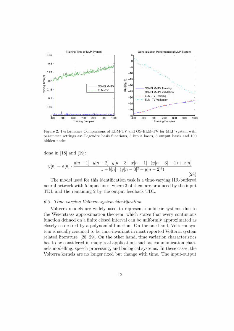
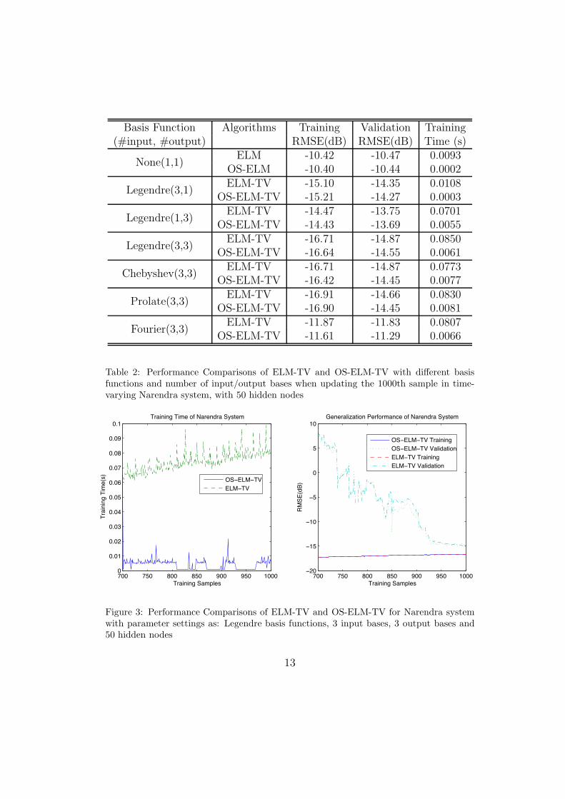
Table 2: Performance Comparisons of ELM-TV and OS-ELM-TV with di!erent basisfunctions and number of input/output bases when updating the 1000th sample in time-varying Narendra system, with 50 hidden nodes

700 750 800 850 900 950 10000

0.01

0.02

0.03

0.04

0.05

0.06

0.07

0.08

0.09

0.1Training Time of Narendra System

Training Samples

Trai

ning

Tim

e(s)

OS ELM TVELM TV

700 750 800 850 900 950 100020

15

10

5

0

5

10

Training Samples

RMSE

(dB)

Generalization Performance of Narendra System


Figure 3: Performance Comparisons of ELM-TV and OS-ELM-TV for Narendra systemwith parameter settings as: Legendre basis functions, 3 input bases, 3 output bases and50 hidden nodes

13

L1 g(·)

x(n) ( y(n)

L2 g(·) $

f(n)

1 # #

#

Figure 4: Nonlinear nonstationary system with one stationary and one nonstationarybranch

relationship of a time-varying Volterra system can be described as [30]:

y(n) =k0(n) +M"

m1=0

k1(n; m1)x(n # m1)

+M"

m1=0

M"

m2=0

k2(n; m1, m2)x(n # m1)x(n # m2) + . . . (29)

where {ki} are the time-varying Volterra kernels and M is the memory lengthof the system.

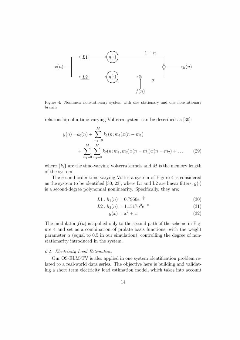
The second-order time-varying Volterra system of Figure 4 is consideredas the system to be identified [30, 23], where L1 and L2 are linear filters, g(·)is a second-degree polynomial nonlinearity. Specifically, they are:

L1 : h1(n) = 0.7950e"n2 (30)

L2 : h2(n) = 1.1517n2e"n (31)

g(x) = x2 + x. (32)

The modulator f(n) is applied only to the second path of the scheme in Fig-ure 4 and set as a combination of prolate basis functions, with the weightparameter # (equal to 0.5 in our simulation), controlling the degree of non-stationarity introduced in the system.

6.4. Electricity Load Estimation

Our OS-ELM-TV is also applied in one system identification problem re-lated to a real-world data series. The objective here is building and validat-ing a short term electricity load estimation model, which takes into account

14


None(1,1)ELM -6.667 0.5344 0.0564

OS-ELM -6.682 0.6433 0.0065

Legendre(3,1)ELM-TV -9.071 0.1897 0.0579

OS-ELM-TV -9.151 -0.3696 0.0053

Legendre(1,4)ELM-TV -11.43 -4.141 0.9128

OS-ELM-TV -11.20 -3.699 0.0102

Legendre(3,4)ELM-TV -12.97 -2.508 1.0048

OS-ELM-TV -12.66 -2.235 0.0111

Chebyshev(1,4)ELM-TV -11.45 -4.089 0.9929

OS-ELM-TV -11.45 -3.887 0.0104

Prolate(1,4)ELM-TV -14.27 -4.723 0.8397

OS-ELM-TV -14.44 -4.450 0.0106

Fourier(1,4)ELM-TV -11.22 -0.634 0.8800

OS-ELM-TV -11.22 -0.861 0.0109

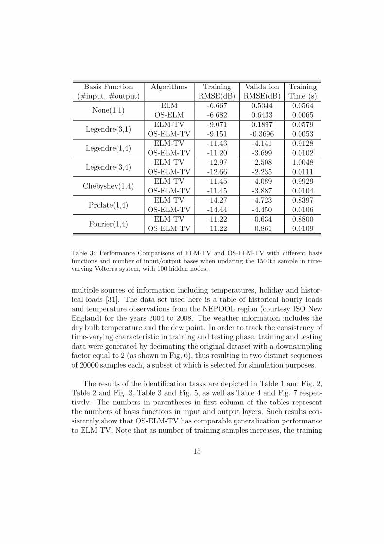
Table 3: Performance Comparisons of ELM-TV and OS-ELM-TV with di!erent basisfunctions and number of input/output bases when updating the 1500th sample in time-varying Volterra system, with 100 hidden nodes.

multiple sources of information including temperatures, holiday and histor-ical loads [31]. The data set used here is a table of historical hourly loadsand temperature observations from the NEPOOL region (courtesy ISO NewEngland) for the years 2004 to 2008. The weather information includes thedry bulb temperature and the dew point. In order to track the consistency oftime-varying characteristic in training and testing phase, training and testingdata were generated by decimating the original dataset with a downsamplingfactor equal to 2 (as shown in Fig. 6), thus resulting in two distinct sequencesof 20000 samples each, a subset of which is selected for simulation purposes.

The results of the identification tasks are depicted in Table 1 and Fig. 2,Table 2 and Fig. 3, Table 3 and Fig. 5, as well as Table 4 and Fig. 7 respec-tively. The numbers in parentheses in first column of the tables representthe numbers of basis functions in input and output layers. Such results con-sistently show that OS-ELM-TV has comparable generalization performanceto ELM-TV. Note that as number of training samples increases, the training

15

1200 1300 1400 15000

0.2

0.4

0.6

0.8

1

1.2

1.4Training Time of Volterra System

Training Samples

Trai

ning

Tim

e(s)

OS ELM TVELM TV

1200 1300 1400 150015

10

5

0

Training SamplesRM

SE(d

B)

Generalization Performance of Volterra System


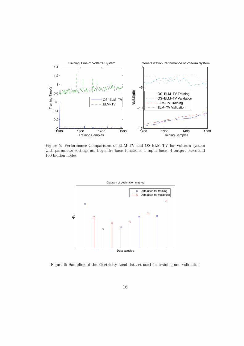
Figure 5: Performance Comparisons of ELM-TV and OS-ELM-TV for Volterra systemwith parameter settings as: Legendre basis functions, 1 input basis, 4 output bases and100 hidden nodes

Data samples

x[n]

Diagram of decimation method

Data used for trainingData used for validation

Figure 6: Sampling of the Electricity Load dataset used for training and validation

16


None(1,1)ELM -14.84 -14.83 0.0123

OS-ELM -14.66 -14.64 0.0002

Legendre(3,1)ELM-TV -12.90 -12.90 0.0173

OS-ELM-TV -12.90 -12.91 0.0003

Legendre(1,3)ELM-TV -15.74 -15.69 0.0616

OS-ELM-TV -15.45 -15.41 0.0004

Legendre(3,3)ELM-TV -13.98 -13.92 0.0781

OS-ELM-TV -14.07 -14.03 0.0004

Chebyshev(1,3)ELM-TV -15.62 -15.60 0.0656

OS-ELM-TV -15.60 -15.59 0.0004

Prolate(1,3)ELM-TV -15.74 -15.71 0.0679

OS-ELM-TV -15.69 -15.67 0.0004

Fourier(1,3)ELM-TV -15.41 -15.40 0.0607

OS-ELM-TV -15.32 -15.30 0.0004

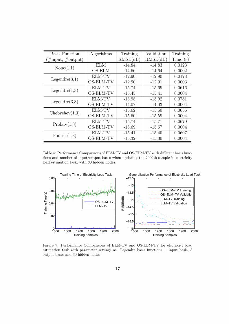
Table 4: Performance Comparisons of ELM-TV and OS-ELM-TV with di!erent basis func-tions and number of input/output bases when updating the 2000th sample in electricityload estimation task, with 30 hidden nodes.

1500 1600 1700 1800 1900 20000

0.02

0.04

0.06

0.08Training Time of Electricity Load Task

Training Samples

Trai

ning

Tim

e(s)

OS ELM TVELM TV

1500 1600 1700 1800 1900 200016

15.5

15

14.5

14

13.5

13

12.5

Training Samples

RMSE

(dB)

Generalization Performance of Electricity Load Task


Figure 7: Performance Comparisons of ELM-TV and OS-ELM-TV for electricity loadestimation task with parameter settings as: Legendre basis functions, 1 input basis, 3output bases and 30 hidden nodes

17

RMSE value becomes worse, because more training samples mean more rowsin G and T, hence more equations to be satisfied in (10) and thus an increas-ing value of the term "G!# T". However, the validation RMSE turns outto be better, as expected: the more the network is trained (if no overfittingoccurs), the better it can identifies the target systems.

On the other hand, OS-ELM-TV consumes much less training time whenupdating the output weights in the applications in which the training data setarrived sequentially. Especially in the case of large number of hidden nodesand large number of output bases, as shown in Table 3 and Fig. 5 for Volterrasystem identification task: once the TV-NN receives a new training sample,OS-ELM-TV takes only about 0.01 seconds to update its output weights,while ELM-TV takes more than 0.8 seconds to retrain its network; as well asin Table 4 and Fig. 7 for electricity load estimation task, 0.4 milliseconds inOS-ELM-TV versus 60 milliseconds in ELM-TV. Moreover, it can be easilyobserved from Fig. 2, 3, 5, 7 that the training time at the starting point N0

of OS-ELM-TV is similar to that of ELM-TV, since their computation loadis equivalent at N0.

Although there are no memory requirements results explicitly shown inthe simulations, we can briefly notice that ELM-TV simply runs out of mem-ory when N comes to 105, while OS-ELM-TV is still able to work.

Last but not least, it is noteworthy to underline that in all tasks thenonstationary ELM approaches lead to significant system identification per-formance improvements w.r.t. the stationary counterpart (denoted by the“None” designation in Tables), both in the batch and in the sequential onlinecase studies. This confirms the trend already observed in previous publica-tions.

7. Conclusions

In this contribution, the authors have extended the online sequential Ex-treme Learning Machine to train Time-Varying Neural Networks, giving ori-gin to the new algorithm namely OS-ELM-TV. The proposed technique isoriented to applications with sequential arrival or large number of trainingdata set. The main advantage of the online approach consists in updatingthe output weights with much less time when new training data arrived, orconsuming less memory if large number of samples have to be trained. Ithas to be noted that this issue is surely much more relevant in the TV-NNcase study, where the presence of time-varying synapses increases the overall

18

number of free parameters w.r.t. standard time-invariant NN. Simulationresults showed that with the benefits discussed above, OS-ELM-TV achievedcomparable generalization performances to ELM-TV. It has also to be ob-served that the OS-ELM-TV behavior perfectly matches with that one ofthe original OS-ELM [14], working in stationary environments, allowing usto positively conclude about the e!ectiveness of the proposed generalizationto the time-varying neural network case study.

Future works are first oriented to enlarge the applicability of the ELMparadigm in real-world nonstationary environments. Moreover some e!ortsare actually on-going in combining the sequential approach with the incre-mental one, already investigated by the authors [21, 22] and allowing to au-tomatize the selection of number of hidden nodes and basis function withinthe training algorithm.

References

[1] G.-B. Huang, Q.-Y. Zhu, C.-K. Siew, Extreme learning machine: Theoryand applications, Neurocomputing 70 (1-3) (2006) 489 – 501, neuralNetworks - Selected Papers from the 7th Brazilian Symposium on NeuralNetworks (SBRN ’04).

[2] Q.-Y. Zhu, A. Qin, P. Suganthan, G.-B. Huang, Evolutionary extremelearning machine, Pattern Recognition 38 (10) (2005) 1759 – 1763.

[3] G.-B. Huang, L. Chen, C.-K. Siew, Universal approximation using in-cremental constructive feedforward networks with random hidden nodes,IEEE Transactions on Neural Networks 17 (4) (2006) 879–892.

[4] G. Huang, L. Chen, Enhanced random search based incremental extremelearning machine, Neurocomputing 71 (16-18) (2008) 3460–3468.

[5] G. Feng, G.-B. Huang, Q. Lin, R. Gay, Error Minimized Extreme Learn-ing Machine With Growth of Hidden Nodes and Incremental Learning,IEEE Transactions on Neural Networks 20 (8) (2009) 1352 –1357.

[6] S. Suresh, S. Saraswathi, N. Sundararajan, Performance enhancementof extreme learning machine for multi-category sparse data classifica-tion problems, Engineering Applications of Artificial Intelligence 23 (7)(2010) 1149–1157.

19

[7] E. Soria-Olivas, J. Gomez-Sanchis, J. Martin, J. Vila-Frances, M. Mar-tinez, J. Magdalena, A. Serrano, BELM: Bayesian Extreme LearningMachine, IEEE Transactions on Neural Networks 22 (3) (2011) 505 –509.

[8] Y. Miche, A. Sorjamaa, P. Bas, O. Simula, C. Jutten, A. Lendasse, OP-ELM: Optimally pruned extreme learning machine, IEEE Transactionson Neural Networks 21 (1) (2010) 158–162.

[9] J. Cao, Z. Lin, G. Huang, Composite function wavelet neural networkswith extreme learning machine, Neurocomputing 73 (7-9) (2010) 1405–1416.

[10] F. Han, D.-S. Huang, Improved extreme learning machine for func-tion approximation by encoding a priori information, Neurocomputing69 (16-18) (2006) 2369 – 2373.

[11] D. Huang, Radial basis probabilistic neural networks: Model and ap-plication, International Journal of Pattern Recognition and ArtificialIntelligence 13 (1999) 1083–1101.

[12] D.-S. Huang, J.-X. Du, A Constructive Hybrid Structure Optimiza-tion Methodology for Radial Basis Probabilistic Neural Networks, IEEETransactions on Neural Networks 19 (12) (2008) 2099 –2115.

[13] G. Huang, C. Siew, Extreme learning machine: RBF network case, in:Control, Automation, Robotics and Vision Conference, 2004. ICARCV2004 8th, Vol. 2, IEEE, 2004, pp. 1029–1036.

[14] N.-Y. Liang, G.-B. Huang, P. Saratchandran, N. Sundararajan, A Fastand Accurate Online Sequential Learning Algorithm for FeedforwardNetworks, IEEE Transactions on Neural Networks 17 (6) (2006) 1411–1423.

[15] M.-B. Li, M. J. Er, Nonlinear System Identification Using ExtremeLearning Machine, in: Proc. 9th International Conference on Control,Automation, Robotics and Vision ICARCV ’06, 2006, pp. 1–4.

[16] Y. Xu, Z. Dong, K. Meng, R. Zhang, K. Wong, Real-time transientstability assessment model using extreme learning machine, Generation,Transmission & Distribution, IET 5 (3) (2011) 314–322.

20

[17] D. Percival, A. Walden, Spectral analysis for physical applications: mul-titaper and conventional univariate techniques, Cambridge Univ Pr,1993.

[18] A. Titti, S. Squartini, F. Piazza, A new time-variant neural based ap-proach for nonstationary and non-linear system identification, in: Proc.IEEE International Symposium on Circuits and Systems ISCAS 2005,2005, pp. 5134–5137.

[19] C. Cingolani, S. Squartini, F. Piazza, An extreme learning machine ap-proach for training Time Variant Neural Networks, in: Proc. IEEE AsiaPacific Conference on Circuits and Systems APCCAS 2008, 2008, pp.384–387.

[20] Y. Ye, S. Squartini, F. Piazza, A Group Selection Evolutionary Ex-treme Learning Machine Approach for Time-Variant Neural Networks,in: Neural Nets WIRN10: Proceedings of the 20th Italian Workshop onNeural Nets, IOS Press, 2011, pp. 22–33.

[21] Y. Ye, S. Squartini, F. Piazza, Incremental-Based Extreme LearningMachine Algorithms for Time-Variant Neural Networks, Advanced In-telligent Computing Theories and Applications (2010) 9–16.

[22] Y. Ye, S. Squartini, F. Piazza, ELM-Based Time-Variant Neural Net-works with Incremental Number of Output Basis Functions, Advancesin Neural Networks–ISNN 2011 (2011) 403–410.

[23] Y. Ye, S. Squartini, F. Piazza, ELM-based Algorithms for NonstationaryVolterra System Identification, in: Neural Nets WIRN11: Proceedingsof the 21st Italian Workshop on Neural Nets, IOS Press, Accepted.

[24] Y. Grenier, Time-dependent ARMA modeling of nonstationary signals,IEEE Transactions on Acoustics, Speech and Signal Processing 31 (4)(1983) 899–911.

[25] R. Horn, C. Johnson, Topics in matrix analysis, Cambridge UniversityPress, 1994.

[26] G. Golub, C. Loan, Matrix computations, 3rd ed, Johns Hopkins studiesin the mathematical sciences, Johns Hopkins University Press, 1996.

21

[27] K. Narendra, K. Parthasarathy, Identification and control of dynamicalsystems using neural networks, IEEE Transactions on Neural Networks1 (1) (1990) 4 –27.

[28] L. Azpicueta-Ruiz, M. Zeller, A. Figueiras-Vidal, J. Arenas-Garcia,W. Kellermann, Adaptive Combination of Volterra Kernels and Its Ap-plication to Nonlinear Acoustic Echo Cancellation, IEEE Transactionson Audio, Speech, and Language Processing 19 (1) (2011) 97 –110.

[29] G. Glentis, P. Koukoulas, N. Kalouptsidis, E"cient algorithms forVolterra system identification, IEEE Transactions on Signal Processing47 (11) (1999) 3042–3057.

[30] M. Iatrou, T. Berger, V. Marmarelis, Modeling of nonlinear nonstation-ary dynamic systems with a novel class of artificial neural networks,IEEE Transactions on Neural Networks 10 (2) (1999) 327–339.

[31] A. Deoras, Electricity Load and Price Forecasting Webinar Case Study(2010).URL http://www.mathworks.com/matlabcentral/fileexchange/28684-electricity-load-and-price-forecasting-webinar-case-study

22

Documents

Online sequential extreme learning machine in nonstationary environments