Parallel Computing 15 (1990) 61-74 61 North-Holland

A paral le l F F T on an M I M D m a c h i n e *

Amir AVERBUCH t, Eran GABBER f, Boaz GORDISSKY t and Yoav MEDAN *

t Department of Computer Science, School of Mathematical Sciences, TeI.Aviv University, Tel-Avic 69978, Israel Science and Technology, 1BM Israel Ltd, Technion city, Haifa 32000, Israel

Received December 1989

Abstract. In this paper we present a parallelization of the Cooley-Tukey FFT algorithm that is implemented on a shared-memory MIMD (non-vector) machine that was built in the Dept. of Computer Science, Tel Aviv University. A parallel algorithm is presented for one dimension Fourier transform with performance analysis. For a large array of complex numbers to be transformed, an almost linear speed-up is demonstrated. This algorithm can be executed by any number of processors, but generally the number is much less than the length of the input data.

Keywords. Parallel algorithm, Parallel FFT, Shared-memory MIMD machine.

1. Introduction

The Discrete Fourier Transform (DFT) and its accelerated version, the Fast Fourier Transform (FFT), has become a necessary tool in many various scientific and engineering applications. Since its introduction [1] in 1965 it is a target for an extensive research to implement an efficient FFT on general purpose, serial and parallel, machines and on special hardware. The FFT is an ideal candidate to be implemented on a vector processor by careful pipelining and scheduling of the stages of the computation.

The FFT algorithm implementation, written in a high-level source language, is specifically tailored for a particular architecture. Nevertheless, it can be easily implemented on a vector processor since the idea for this implementation came from a successful vectorization of the F F T [12,16] which achieved the full potential speed of vector processors. We will demonstrate very clearly that the architecture dependent parameters are a major factor in speeding up the computation. The main result is that for large arrays (i.e. 64K or greater), the speedup is almost linear. However, if the number of array elements to be transformed is below some threshold, then there is almost no speedup.

This paper is organized as follows. In Section 2 we review the various existing architectures on which the F FT has been implemented. In Section 3 we present the parallel one dimensional F F T algorithm. There we present a parallel algorithm with four stages to perform the F F T in parallel. In Section 4 we describe the 1-dimensional Generalized F F T (GFFT) which includes the DFT as a particular case. The parallel one-dimensional G F F T is the algorithm we implemented on our parallel machine. The machine architecture and the specific implementa- tion is described in Section 5. We describe the associated hardware and software architecture that we utilize. In addition to the implementation description we detail the integration of the

* This work was supported by the Basic Research Foundation administered by the Israeli Academy of Sciences and part by a research grant from National Semiconductor, Israel. Short version of the paper appeared in the 1989 International Coneference on Parallel Processing, pp. 111-63-Ill-70, August 8-12, 1989, Chicago.

0167-8191/90/$03.50 © 1990 - Elsevier Science Publishers B.V. (North-Holland)

62 A. Averbuch et al. / Parallel F F T on an M I M D machine

algorithm and the architecture, give a high-level description of the implementation whith an emphasis on the relationship amongst the algorithm and the shared bus & shared memory architecture in order to obtain an optimal performance. The features that compromise a good match between the architecture and the algorithm are described. We will address computational issues such as memory strides, vector length, communication overhead. In Section 6 we review and analyze the results based on execution speeds of various sizes of one dimensional F F T and in Section 7 we present the performance analysis based on the match between the algorithm and the M I M D architecture.

2. Vector and muitiprocessor FFTs

The FFT is an ideal candidate to be implemented on a vector processor. Its structure, which is mainly a computation of an inner product between vectors, is perfectly suitable to most commercially available vector processors. There is a substantial amount of literature on this subject [4-7,12,15-16], to name a few. The vectored realizations of the F F T are the main source for the new ideas for the proposed implementation of the F F T on multiprocessors.

References [2] and [3] provide a review of several multiprocessor FFTs that were developed for multiprocessor (and vector multiporcessors) with shared memory and multiprocessors with message passing.

A large variety of multiprocessors exist today and they can be grossly classified as either shared memory or message passing. All inter-processor communication in a shared-memory architecture is done through shared memory. The shared memory may hold global data, be used to emulate message passing, or to store local results. The shared memory may be either uniformly accessed from all processors, divided among processor clusters, or form a hierarchy. The F F T was implemented on the IBM RP3 [10-11] which is a shared memory multiprocessor, and the multiprocessors are connected to shared memory by a multistage interconnection network. In [3] there is an implementation of the FFT on an A L L I A N T F X / 8 which is a vector multiprocessor. The vector multiprocessors consist of several vector processors connected to shared memory processor.

All inter-communication in a message passing architecture is done by message passing through communication links. Each processor has some local memory. Common data must be duplicated in all processors because there is no shared memory that is globally accessible. The Hypercube is an example of such an architecture. In [3] there is an analysis of a hypercube FFT. [8-9] do not specifically discuss the FFT but they focus on the communication complexity of the general algorithms on the hypercube.

Recently, parallel algorithms for one and two-dimensional FFT over a wide variety of interconnection networks were considered in [21] except a binary tree. The problem of computing the two-dimensional FFT on a tree-structured parallel computer is addressed in [22].

3. 1-dimensional parallel FFT

Let {x(n) : 0 < n ~< N - 1} be N samples of a time function. The D F T is defined

N--1

X ( k ) = ~_, x(n)WkN '~ O < ~ k < ~ N - 1 W N = e -'2~'/N (1) n = 0

As we mentioned in Section 2, most of the nlultiprocessor FFT implementations are based on the vector realization of the FFT. Our algorithm is a modification of [15] which is a fully

A. Averbuch et a L / Parallel FFT on an MIMD machine 63

vectorized mixed-radix algori thm, that does not require any special tor operat ions. This yields the current modif ica t ion and implementa t ion on our sha red -memory paral le l M I M D machine.

Assume that

N = N a . . . . . N o. (2)

Conceptual ly , we can think of a one-dimensional a r ray x of d imension N to be a p -d imen- sional array x ' of d imension N o × N o_ 1 × " " " × N1. Tha t is

x ' ( n o . . . . . n, . . . . . n , ) = x ( n o + n e _ l N o + . . . naN2N3 " " No) (3)

n i = 0 , 1 . . . . . N , - 1 i = 1 , 2 . . . . .

The first step of the a lgori thm is an " index reversal" which is general izat ion of " b i t reversal". In our case, this corresponds to a p-d imens iona l t ransposit ion. Therefore, we define another p-d imens iona l a r ray x 0 in th following way:

X o ( n , . . . . . np) = x ' ( n p . . . . . n~). (4)

This step is done in parallel. F r o m (3) we have that

XO(H 1 . . . . . Hp) = x ( np + n o _ , N p + . . . + n , N z N 3 . . . N o ) . (5)

We treat the array X of length n as a p-d imensional a r ray x o

Xp( k, . . . . . k p ) = X ( k , + N , k 2 + " " + g l N 2 " " N o _ , k p ) (6)

k i = 0 . . . . . N , - 1 i = 1 . . . . . p .

No te that Xp and X are equivalent arrays. Subst i tut ing (5) and (6) in (1), we obta in

x p ( k l , . . . , k p ) = E xo (n l . . . . . n p ) W N fpgp (7) n l , n 2 , . . . , np

where

and

f , = , , , + ,, o _ , U p + . . . , , , N 2 N 3 . . . U~

gp = k l + N l k 2 + " '" +NIN2 " ' " N p - a k p

and the general definit ion of these functions is

~ = f j ( n , , n 2 . . . . . n j ) = n j + n j _ , N j + . . . + n , N 2 N 3 . . . N j

and

Def ine

g j = g j ( k , , 1,~ . . . . . kj) =k, +N,k~+--. +N,N~ . . . Nj_ ,k j

j = l . . . . . p

L j = N 1 N z . . . N j j = l , 2 . . . . . p .

(9a) and (9b) can be wri t ten recursively using (10) as:

f, = . j +f,_,~ g j = g j _ , + L j _ , l , r

F r o m the above

~gj

(8a)

(8b)

(9a)

(9b)

(10)

(11)

Def ine f0 = go = 0 and L 0 = 1. F r o m [3] and the above, the D F T of (1) can be pe r fo rmed in

f j - l g j - 1 n j g j - i n j k j Lj - f J - l k J + L j ~ _ 1 + - - - ~ j + - ~ - - j j = l . . . . . p . (12)

64 A. Averbuch et a L / Parallel FFT on an MIMD machine

j = 1 . . . . . p successive stages in which N/Ny, one-dimensional DFT's of Xj, of length Nj, are performed along the rows of the partially transformed Xj_I:

Nj-1

X i ( K j ) = Y'. X j - I ( K j _ I ) W [ / g : - ' W ~ jkj (13) nj= 0

where

g j = r / j + 1 . . . . , n p , k I . . . . , kj J

L,= VIN, I=1

J gj= E k t L , - i ( L o = l )

1=1

% = 0 . . . . . Nj-1

and Xo(Ko) is obtained from x(n) by an "index-reversal" transformation. At the end of the p th stage, X(k) = Xp(Kp).

In (13), the second term represents the twiddle factor scaling the j t h stage [15]. The last term represents the DFT's of length Nj.

If a vector of length N that has to be transformed can be represented as a p-dimensional array where N = N1N2... Np then the DFT of the vector can be done in p successive stages where each stage consists of the following phases:

1. Load N/Ny vectors of length Nj.. 2. Do N/Nj - 1 vector multiplications using N/Nj - 1 pre-computed twiddle factor vectors. 3. Compute the radix-Nj vector DFT. 4. Store N/Nj vectors. In phase 2 of the algorithm we have to compute the twiddle factor, i.e. w~JgJ -, j = 1 ..... p

(13), but a new technique is presented in the next section to incorprate the computation of the twiddle factor into the computation of the FFT which will yield a 3-step parallel FFT. Such a DF T is called a Generalized FFT.

4. 1-dimensional FFT and Generalized FFF (GFFT)

The one dimensional Discrete Fourier Transform (DFT) of a finite series ( x (n ) : 0 ~< n ~ N - 1 } (real or complex) is the complex series given by

N - - 1

X ( k ) = Y~. x(n)W~ n O<<.k<~N-1 Ws=e -'2,/N. (14) n = 0

The number of complex multiplications for a DFT of N points when N = 2" is (N/2) log 2 N. Here we are introducing one type of FFT which is called decimation in time by using the "basic butterfly operation":

N X~c(k) = GN/2(k ) + W~HN/2(k ) 0 ~ k ~ -~- - 1 (15a)

, , x N k + = - 0 k - 1 (15b)

where

GN/2(k) =

N - - - - 1 2

E (2m) m = O

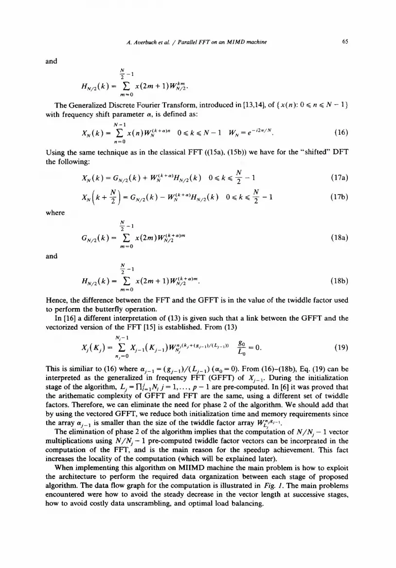
A. Averbuch et a L / Parallel F F T on an M I M D machine 65

and N - - - 1 2

HN/z(k ) = Y'. x(Zm + 1)W;*/"~. m ~ O

The Generalized Discrete Fourier Transform, introduced in [13,14], of { x (n): 0 ~< n ~< N - 1 } with frequency shift parameter a, is defined as:

N--1

X N ( k ) = ~_, x(n)W(N k+')" O<~k<~N-1 WN=e -i2"/N. (16) n = 0

Using the same technique as in the classical F F T ((15a), (15b)) we have for the "shifted" D F T the following:

N XN(k ) = Gu/2(k ) + W(uk+")HN/z(k) 0 ~< k ~< y - 1 (17a)

XN( k + N ) = Gu/2( k ) _ w(k +'~)14 it.-, N "N --u/2~'- i 0 ~ < k ~ < ~ - - 1 (17b)

where

and

N - - - - 1 2

Gu/2(k ) = ~., x(2m)W(N~; ")m (18a) m~O

N - - - - 1 2

Hu/: (k ) = ~_, x (2m + 1)WN(~ -" ) ' . (18b) m ~ 0

Hence, the difference between the FFT and the G F F T is in the value of the twiddle factor used to perform the butterfly operation.

In [16] a different interpretation of (13) is given such that a link between the G F F T and the vectorized version of the FFT [15] is established. From (13)

Xj(Kj)= E Xj-,(Kj-, W g°=0. (19) j uj Lo nj=O

This is similiar to (16) where aj_ 1 = (g j_O/ (L j_O (a 0 = 0). From (16)-(18b), Eq. (19) can be interpreted as the generalized in frequency F F T (GFFT) of Xj_ 1. During the initialization stage of the algorithm, Lj = l-l[=lN t j = 1 . . . . , p -- 1 are pre-computed. In [6] it was proved that the arithematic complexity of G F F T and FFT are the same, using a different set of twiddle factors. Therefore, we can eliminate the need for phase 2 of the algorithm. We should add that by using the vectored GFFT, we reduce both initialization time and memory requirements since the array %_ 1 is smaller than the size of the twiddle factor array W~JgJ -,.

The elimination of phase 2 of the algorithm implies that the computation of N/Nj - 1 vector multiplications using N / N j - 1 pre-computed twiddle factor vectors can be incorprated in the computation of the FFT, and is the main reason for the speedup achievement. This fact increases the locality of the computation (which will be explained later).

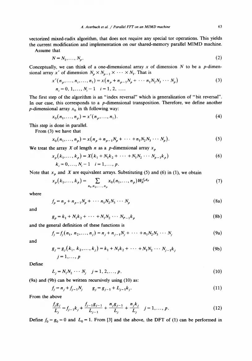
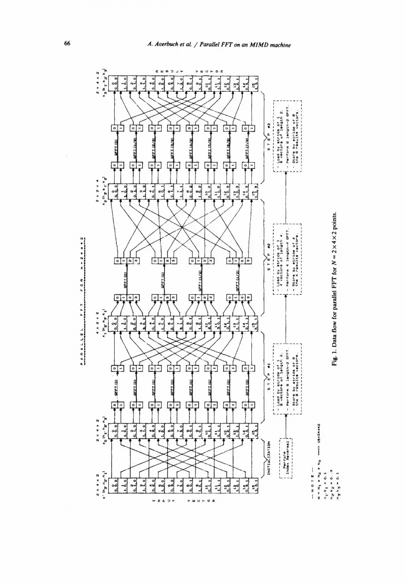
When implementing this algorithm on MIIMD machine the main problem is how to exploit the architecture to perform the required data organization between each stage of proposed algorithm. The data flow graph for the computation is illustrated in Fig. 1. The main problems encountered were how to avoid the steady decrease in the vector length at successive stages, how to avoid costly data unscrambling, and optimal load balancing.

O~

!°

A

R

A

L L

E L

F F

T F

OR

N

-

2 .

4 "

2 ..

....

....

....

....

....

....

....

....

....

....

....

....

..

2 x

4 x

2 2

x 4

x 2

4x

;~x;

~

2 x

2 x

4

x'

(n 3

, n

a,

n 1

) x

0 (n

1.

na

. n

3)

x t

(n 2

, n

3. k

t )

x

2 (n

3

k 1'

kL:

~

0 1

..r

0 "

~ r'

-~

z ~

2 2

- 2

~ I

....

o

l~

/

~ '

L~

J ..

....

....

p 1,

Z,

0 I

\ Y

~

,/ ~

--

--

~/" \

~

;:

~ G

FF

T (

0}

--

~//

U

6 I

\

it

;~

/ .J

~

~ -I

@

6

T 0

13

n 0

0

30

2

t 0

o.

I ~

GF

FT

1

3/8

} -

t,

3,0

t

30

I

3 t.

0

o,o,

..

....

...

c 9

r \

"1

9 9

GF

FT

1

t/2

1

1, o.

l, /V

V 1t

.o'.t

l "L

u '"

",(

N',

]'.1. o

'.t

",:;

.1

1,,

_,,

,.,o.1

X3c-

r-

..

..

..

.

.,

, //

'~./

X

~ .~

rT

L/

....

I,

~~

~

~.

.'

~'

~'

"

~ ~

'-l,

:~.J

, ~'

d it

.a.l

'

t a

t ~

F~

tl,/

a~

-!

'.~

//

~

lt.o

.~

--

/

! 1

5

'%

15

13

. I.

...

.. l

......

1

-IJ_l

~

-~ 1o

p-

""-:

J

S

T ~

E

P

$t

S

T ~

E

P

$2

S

T

E~

/P

$3

I p

erf

op

m

1 I

Ind

ex

Re

vers

e1

I .

..

..

..

..

..

J

2 x

4 x

2

x3{k

t.

k;~

k

3 )

0,0

, o

E S

03

0

U

L T V

E C

T 0

/

( B

vectors

of

length

2.

- Perform

B

length-2

GFFT.

t I - Store

by strlde

of

8

I

the

8 results

vectors.

t .

..

..

..

..

..

..

..

..

..

.

J

F :-L

%;:

~ ~

i:,%

-o3-

; ..

...

t 4

vect

ors

o

f le

ng

th

4.

-

Pe

rfo

rm

4 le

ng

th-4

G

FF

T.

I I - Store

by

strlde

of

4

I th

e

4 re

sult

s ve

cto

rs.

I .

..

..

..

..

..

..

..

..

..

..

r ~-&

;: ~

; ;i:

,~;

%7:

...

. f

8 ve

cto

rs

of

~e

ng

th

2.

i D

I -

Pe

rfo

rm

B

len

gth

--2

G

FF

T.

I I -

Store

by

8tP

~e

Q

f 8

the

e

re~

ult

m

ve

cto

rs.

L .

..

..

..

..

..

..

..

..

..

..

g

--

NO

TE

--

N

--

N1

a

N 2

N

N

3

----

-->

1

6-2

~4

a2

nt"

~

1

--

0,

1

n~

k

2 -

0..

3

n3rk 3 - O, I

Fig

. 1.

Dat

a fl

ow f

or p

aral

lel

FF

T f

or N

=

2 x

4 ×

2 po

ints

.

A. Aoerbuch et al. / Parallel F F T on an M I M D machine 67

5. Implementation

5.1 M M X parallel machine

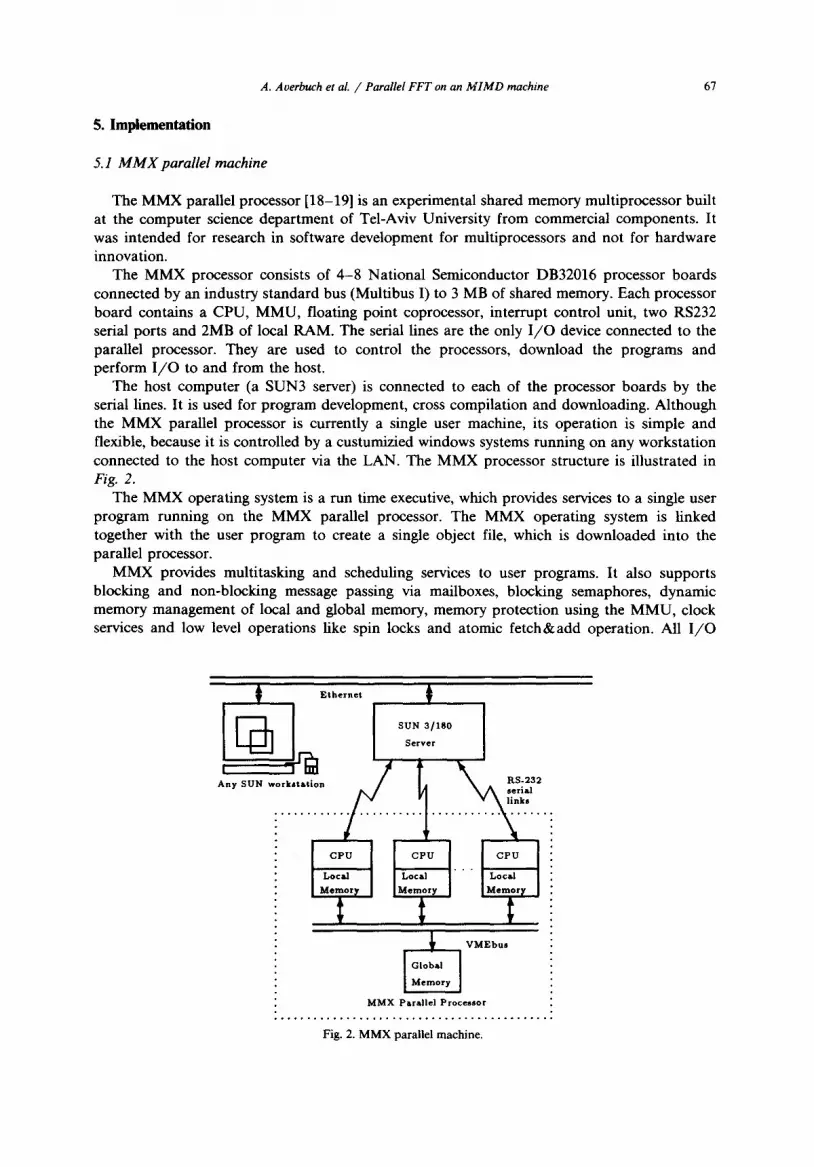
The MMX parallel processor [18-19] is an experimental shared memory multiprocessor built at the computer science department of Tel-Aviv University from commercial components. It was intended for research in software development for multiprocessors and not for hardware innovation.

The MMX processor consists of 4-8 National Semiconductor DB32016 processor boards connected by an industry standard bus (Multibus I) to 3 MB of shared memory. Each processor board contains a CPU, MMU, floating point coprocessor, interrupt control unit, two RS232 serial ports and 2MB of local RAM. The serial lines are the only I / O device connected to the parallel processor. They are used to control the processors, download the programs and perform I /O to and from the host.

The host computer (a SUN3 server) is connected to each of the processor boards by the serial lines. It is used for program development, cross compilation and downloading. Although the MMX parallel processor is currently a single user machine, its operation is simple and flexible, because it is controlled by a custumizied windows systems running on any workstation connected to the host computer via the LAN. The MMX processor structure is illustrated in Fig. 2.

The MMX operating system is a run time executive, which provides services to a single user program running on the MMX parallel processor. The MMX operating system is linked together with the user program to create a single object file, which is downloaded into the parallel processor.

MMX provides multitasking and scheduling services to user programs. It also supports blocking and non-blocking message passing via mailboxes, blocking semaphores, dynamic memory management of local and global memory, memory protection using the MMU, clock services and low level operations like spin locks and atomic fetch&add operation. All I /O

Ethernet

[ Server I

AoySU..ork.,.,,o. h \ ^ . . . . . . . . . . . . . . . .

I I o=

~ VMEbus

M M X Paral le l Processor

Fig. 2. MMX parallel machine.

68 A. Averbuch et al. / Parallel FFT on an MIMD raachme

operations are performed by the GNX run time library, which is supplied by National Semiconductor. It also supports dynamic task creation, automatic load balancing by task migration, tasks synchronization by semaphores, inter-task communication by mailboxes and time-sharing between tasks.

The MMX parallel processor and its operating system has been in constant use since summer 1987. It is now serving more than 10 regular users, who use it for research in software environments, image processing, signal processing and applied mathematics.

5.2 The specific implementation

The algorithm is written in C with MMX services. The performance is optimal when the vectors are equal in length, i.e N = M p (N 1 = N 2 . . . . . Np). The algorithm is performed in p stages, where in each stage N / M G F F T operations are performed on vectors of length M. The N / M G F F T operations are performed in parallel depending on the number of processors. It supports any number of processors.

The parallel program is executed by calling the procedure main _ F F T with the following parameters: N The number of points to be transformed. Mp Decomposition of N to N = M e. log M The number of bits that represents the number M - 1. This is utilized by the "index

reversal" of the input vector. Inverse TR UE to perform Inverse FFT, else FALSE. Vec_real, Vec_image Pointers to real and imaginary parts of the input.

The performance in shared memory & shared bus architecture has been degraded because of the need to access the global memory. This access is done through MULTIBUS which is slower than the bus that is used by the local memory. When a processor wants to access the global memory while the bus is used by another processor then the processor has to wait until the bus is freed. We tried to avoid a frequent use of the global memory. To accomplish the above the following design decisions were taken into consideration:

1. In MMX we can define two types of tasks: Global and local. Global task can reside in any processor and during the execution it can travel from one processor to another. On the other hand, the local task processor-id is predetermined by the program when the local task is generated. During the execution period the local task will reside on this processor. Local task achieves better performance than a global task due to the fact that its stack is located in the local memory which belongs to the processor that executes this task. The emphasis in the implementation was to rely on using the maximum number of local tasks. The following considerations are direct implications of the need to concentrate more on local tasks and local memory.

2. Priority was given to dynamic allocation of memory space in the local memory. 3. We tried to eliminate, as far as possible, the use of global variables. 4. In case a processor necessitates massive access to global memory, then the data in the

global memory is copied to local memory. Then the computation is done in local memory and after completion of the computation the data is moved back to global memory.

5. We tried to eliminate, as far as possible, to use of message-passing among the tasks since message-passing is done through the use of global memory.

5.3 Integration of the algorithm and the architecture

As was explained before, in order to perform one-dimensional F F T of length N = M e the algorithm is performed in p stages where in each stage we performed N / M G F F T operations

M A

I

N

F F

T T

AS

K

I S E

INF R

L' ~L

" ~'T

'E~;I

~N~E

'P~

OZ~ T

ZL

(~J4N

N E

1

I W

AIT ON

SE

MA

RH

O~

|

WH

ILE

STA~

E <

P I

sEN

D "

O0~

FPT"

~

. ~

~

$ ] .

......

......

I

.IT

ON S

EM--O

RE~

.

--•S

EN

D

"TER

MIN

ATE"

M

SS.~I~

I=,

I ...

.. o

....

I

PA

RA

LLE

L F

FT

F

L O

W C

H A

R T

.

S [.

A

V

E F

F T

T A

S

K

[/~0

) ..

....

....

....

....

....

....

....

....

.

I F

FIR

ST

TIM

E O

R NE

W

I

f PE

RFO

RM P

RO

POR

TIO

NAL

t ART

OF

IND

EX R

EVER

SAL

1 ....

......

...

RE I

IF

REC

EIVE

D M

EG -

- "D

O._

FFT"

~E

s

I t.

LO

AD N

/M~T

AEKS

VEC

TORS

I

OF

LEN

GTH

N.

E.

COM

RUTE

NEN

TN

ZDSL

E FA

CTO

RS.

3.

CO

MPU

TE S

FFT

OF

VECT

ORS

4.

STO

RE

BY S

TRID

E O

F N

/M

THE

RES

ULT

VEC

TOR

S.

I ....

......

.....

1 -

NI~

NO

TE fI

N

......

......

......

.. I

-- N

UM

BER

OF

DAT

A PO

INTS

{N

--MNN

F) .

1 ....

......

.....

I

~ES

I. L

OAD

N/M

~TAS

KS V

ECTO

RS

OF

LEN

STH

N.

2. C

OM

PUTE

NEW

TW

IDD

LE

FA

CT

OR

S.

S.

COM

PUTE

GFF

T O

F VE

CTO

RS

4, S

TOR

E BY

STR

IDE

OF

N/M

TH

E R

ESU

LT V

ECTO

RS.

[ ....

......

.....

I

t~ R

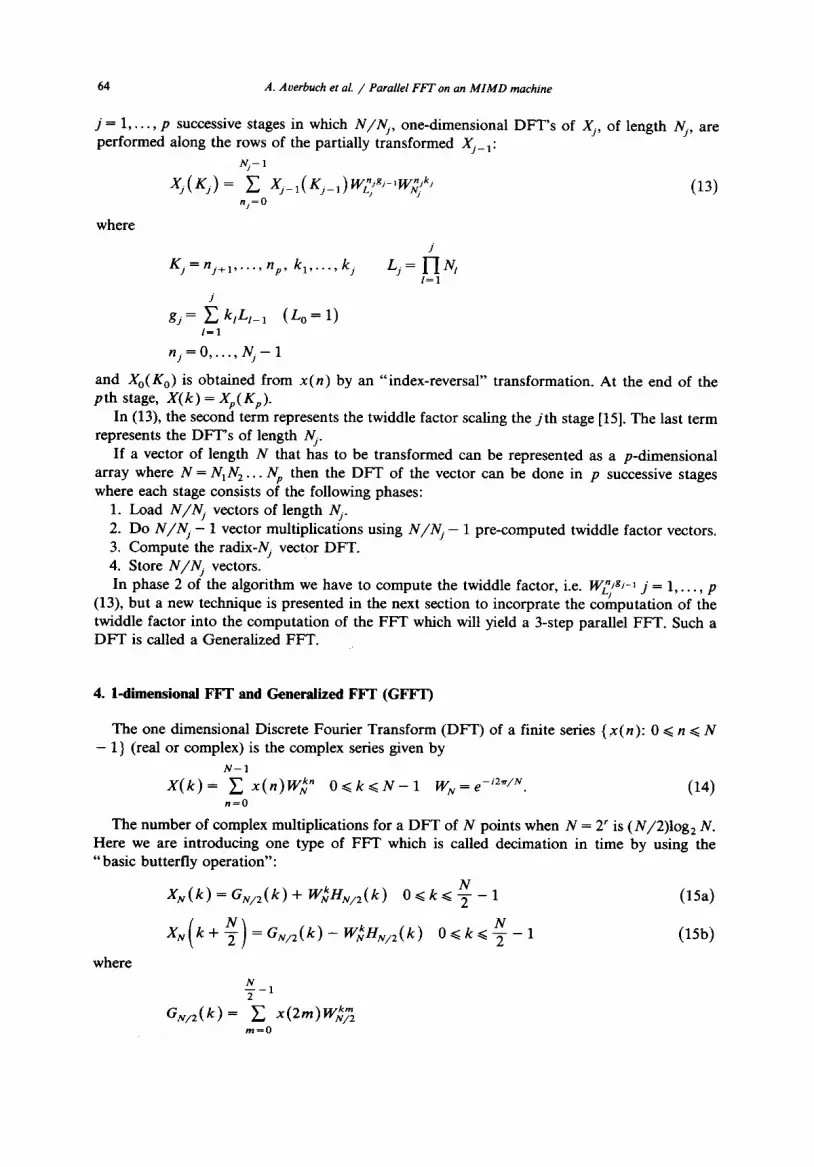
Fig.

3. P

aral

lel

FF

T f

low

char

t. C

~

70 A. Averbuch et al. / Parallel F F T on an M I M D machine

on input vector of length N. These vectors contain the results from the previous stage since the computation is done in place. The N / M input vectors to the G F F T algorithm are generated from reading the input vector while the reading is performed in step 1. The N / M vectors which contain the results of the G F F T in the current stage are written in N / M steps into the output vector which will be the input vector for the next stage.

The N / M operations of the G F F T algorithm are performed in parallel. These operations are independent of each other. Therefore, the number of GFFTs that are performed in parallel in each stage is equal to the number of available processors.

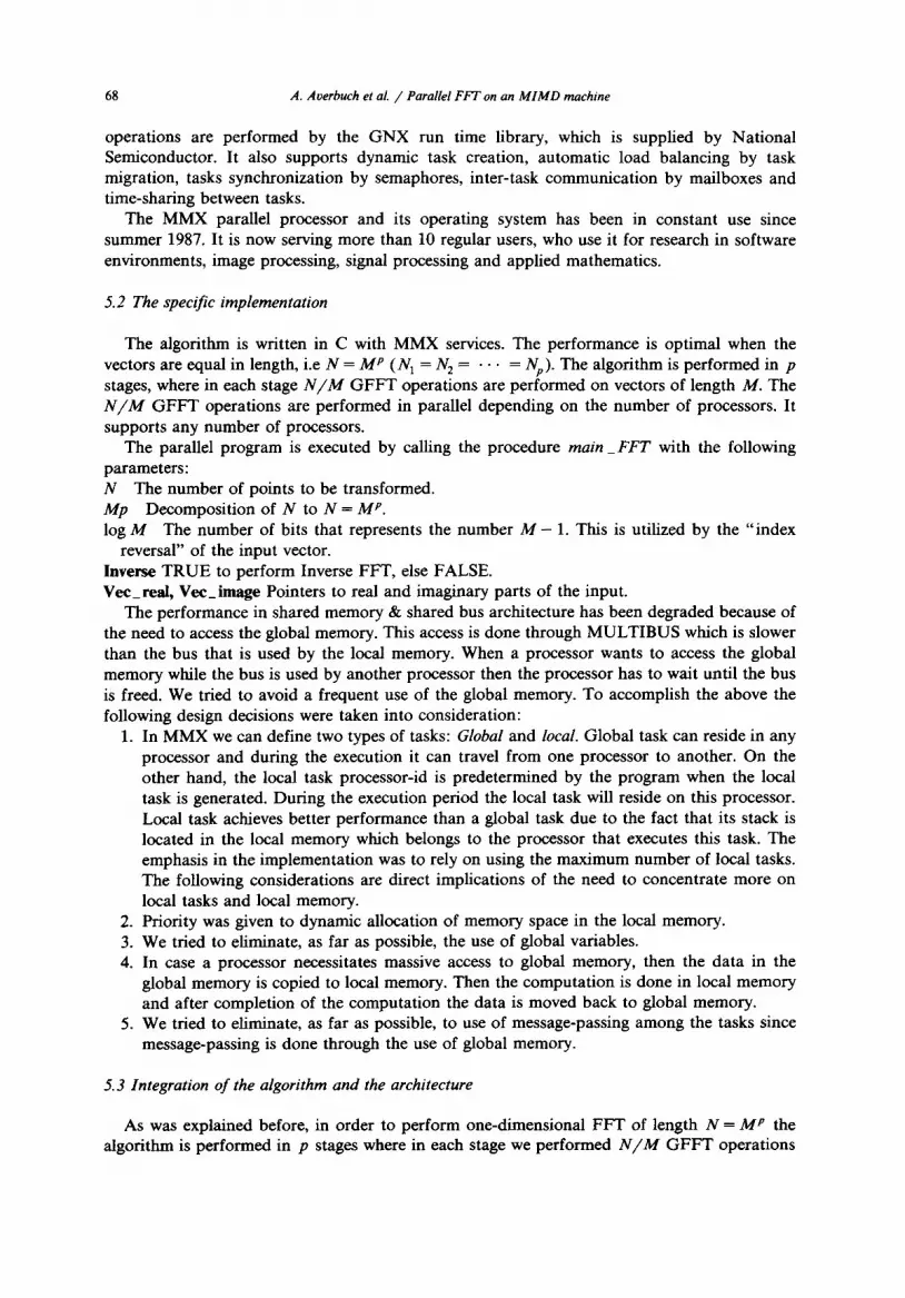
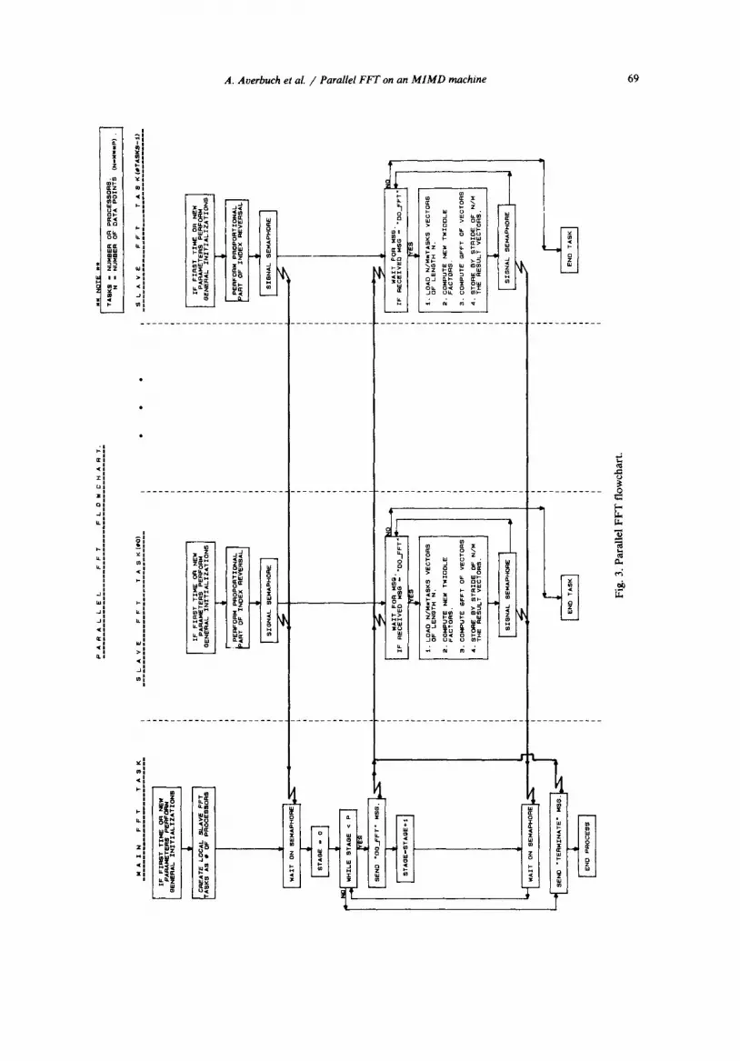
During the execution two main tasks are created M a i n FFT and Slave_FFT (see Fig. 3). 1. Main FFT: Only one task of this type is created. It is the first created task and it generates the rest of

the tasks which are all of type S l a v e FFT. In general, Main _ FFT is used as a "supervisor" and "synchronizer" among the other tasks.

Its main tasks are: • Performs general initializations. • Responsible that the P stages of the algorithm are carried into effect. • Signal the tasks of the type S l a v e FFT to start to execute the next step of the algorithm. • Avoid the situation in which part of the S l a v e FFT starts to execute the next step of the

algorithm while some of them are still busy with the current step of the algorithm. • Perform all kinds of "administrative" types of work like the exchange among input vectors

and output vectors during the completion of the execution in each step of the algorithm. • Take care that the results of the algorithm are written in the user buffers. 2. Slave FFT: The number of available processors dictates the number of Slave FFT. Therefore the

number of Slave_ FFT tasks is equal to the number of processors. These tasks are responsible for the main computational task of the algorithm. In each stage of the P stages algorithm each of the Slave FFT task performs the following:

• Loads N / ( M X #tasks) vectors from the global memory into the local memory (#tasks = #processors).

• Computes for each of these vectors the twiddle factor. • Perform G F F T on each of the vectors. • Stores the results in global memory. In Fig. 3 there is a functional flow-chart that demonstrates the interaction among the tasks

and their responsibilities.

6. Analysis of the results

The parallel F F T has been run on the MMX [18-19] system. To measure the speedup of the parallel F F T we execute a serial FFT on a single 32016 processor. The serial F F T is given without any system service call to MMX. This serial F F T is the fastest version of the F F T we can derive. Transform sizes, which vary from 256 to 65 536 points, have been chosen. The F F T computation is done in radix-2,4 and 8.

The results are given in Tables 1-3. The first column (from left to right) shows the size of vector to be transformed. The other columns contain times for the parallel F F T when it runs on 1 to 4 processors. The speedup, defined as,

serial time s p e e d u p - parallel time

is given under each parallel time. The serial time is given in the rightmost column. The time in

A. Averbuch et al. / Parallel F F T on an M1MD machine 71

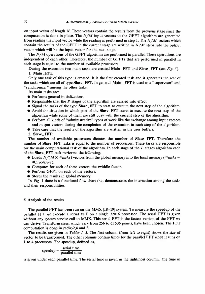
Table 1 FFT radix-2 algorithm timing

# Points Parallel time ( # processors) Serial time

4 3 2 1 (sec.)

256 0.17 0.22 0.28 0.49 0.36 Speed up 2.12 1.64 1.29 512 0.40 0.50 0.70 1.31 0.81 Speed up 2.00 1.62 1.16 1024 0.59 0.83 1.10 2.14 1.77 Speed up 3.00 2.13 1.61 4096 2.43 3.29 4.78 9.45 8.52 Speed up 3.51 2.59 1.78 16384 10.56 14.35 20.91 41.45 39.58 Speed up 3.75 2.76 1.89 65536 45.85 61.06 91.06 180.77 180.15 Speed up 3.93 2.95 1.98

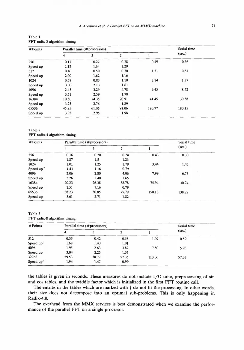
Table 2 FFT radix-4 algorithm timing.

# Points Parallel time ( # processors) Serial time

4 3 2 1 (sec.)

256 0.16 0.20 0.24 0.43 0.30 Speed up 1.87 1.5 1.25 1024 1.01 1.25 1.79 3.44 1.45 Speed up t 1.43 1.16 0.79 4096 2.06 2.80 4.06 7.99 6.73 Speed up 3.26 2.40 1.65 16384 20.23 26.38 38.78 75.94 30.74 Speed up t 1.51 1.16 0.79 65536 38.23 50.85 75.79 150.18 138.22 Speed up 3.61 2.71 1.82

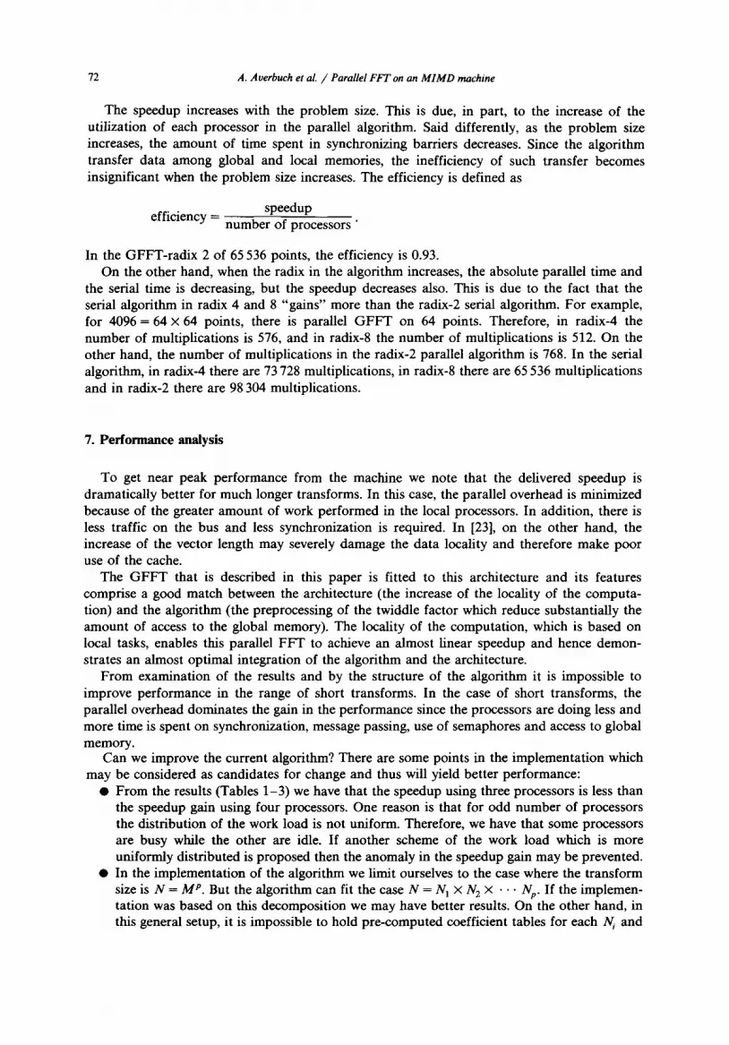
Table 3 FFT radix-8 algorithm timing.

# Points Parallel time (#processors) Serial time

4 3 2 1 (sec.)

512 0.35 0.42 0.58 1.09 0.59 Speed up t 1.68 1.40 1.01 4096 1.95 2.63 3.82 7.50 5.93 Speed up 3.04 2.25 1.55 32768 29.53 38.77 57.35 113.06 57.33 Speed up t 1.94 1.47 0.99

t he t a b l e s is g i v e n in s e c o n d s . T h e s e m e a s u r e s d o n o t i n c l u d e I / O t ime , p r e p r o c e s s i n g o f s in

a n d cos t ab l e s , a n d t he t w i d d l e f a c t o r w h i c h is i n i t i a l i z e d in t h e f i r s t F F T r o u t i n e call .

T h e e n t r i e s in t h e t a b l e s w h i c h a re m a r k e d w i t h ~" d o n o t f i t t h e p r o c e s s i n g . I n o t h e r w o r d s ,

t h e i r size d o e s n o t d e c o m p o s e i n t o a n o p t i m a l s u b - p r o b l e m s . T h i s is o n l y h a p p e n i n g in

R a d i x - 4 , 8 .

T h e o v e r h e a d f r o m t h e M M X serv ices is b e s t d e m o n s t r a t e d w h e n w e e x a m i n e t h e p e r f o r -

m a n c e o f t h e p a r a l l e l F F T o n a s ing le p r o c e s s o r .

72 A. Averbuch et al. / Parallel FFT on an M I M D machine

The speedup increases with the problem size. This is due, in part, to the increase of the utilization of each processor in the parallel algorithm. Said differently, as the problem size increases, the amount of time spent in synchronizing barriers decreases. Since the algorithm transfer data among global and local memories, the inefficiency of such transfer becomes insignificant when the problem size increases. The efficiency is defined as

speedup efficiency = number of processors "

In the GFFT-radix 2 of 65 536 points, the efficiency is 0.93. On the other hand, when the radix in the algorithm increases, the absolute parallel time and

the serial time is decreasing, but the speedup decreases also. This is due to the fact that the serial algorithm in radix 4 and 8 "gains" more than the radix-2 serial algorithm. For example, for 4096 = 64 × 64 points, there is parallel G F F T on 64 points. Therefore, in radix-4 the number of multiplications is 576, and in radix-8 the number of multiplications is 512. On the other hand, the number of multiplications in the radix-2 parallel algorithm is 768. In the serial algorithm, in radix-4 there are 73 728 multiplications, in radix-8 there are 65 536 multiplications and in radix-2 there are 98 304 multiplications.

7. Performance analysis

To get near peak performance from the machine we note that the delivered speedup is dramatically better for much longer transforms. In this case, the parallel overhead is minimized because of the greater amount of work performed in the local processors. In addition, there is less traffic on the bus and less synchronization is required. In [23], on the other hand, the increase of the vector length may severely damage the data locality and therefore make poor use of the cache.

The G F F T that is described in this paper is fitted to this architecture and its features comprise a good match between the architecture (the increase of the locality of the computa- tion) and the algorithm (the preprocessing of the twiddle factor which reduce substantially the amount of access to the global memory). The locality of the computation, which is based on local tasks, enables this parallel FFT to achieve an almost linear speedup and hence demon- strates an almost optimal integration of the algorithm and the architecture.

From examination of the results and by the structure of the algorithm it is impossible to improve performance in the range of short transforms. In the case of short transforms, the parallel overhead dominates the gain in the performance since the processors are doing less and more time is spent on synchronization, message passing, use of semaphores and access to global memory.

Can we improve the current algorithm? There are some points in the implementation which may be considered as candidates for change and thus will yield better performance:

• From the results (Tables 1-3) we have that the speedup using three processors is less than the speedup gain using four processors. One reason is that for odd number of processors the distribution of the work load is not uniform. Therefore, we have that some processors are busy while the other are idle. If another scheme of the work load which is more uniformly distributed is proposed then the anomaly in the speedup gain may be prevented.

• In the implementation of the algorithm we limit ourselves to the case where the transform size is N = M p. But the algorithm can fit the case N = N 1 × N 2 x • • • Np. If the implemen- tation was based on this decomposition we may have better results. On the other hand, in this general setup, it is impossible to hold pre-computed coefficient tables for each N~ and

A. Averbuch et al. / Parallel F F T on an M I M D machine 73

therefore we are forced to get them from the on-line computation of the mathematical functions sin and cos which may degrade the performance. But a potential algorithm for a mix-radix G F F T is given by the following analysis. If we denote by */ the ratio between the computational complexity of the twiddle factor array and that of the frequency shift array, we have

P L 1) Ej=I j - I(Nj - (20)

-- Ef=lLj_ l - 1

Eq. (20) can be easily reduced to the following form:

L p - 1 Np

71 = ~ f = 1 L j _ I _ 1 --- Np N p _ l .

An approximate upper limit for ,/ is given by:

Up . . . . . (21) ~ -~ Np - Np_ l

According to Eqs. (20-21) it can be concluded that: - To increase the efficiency of a mixed-radix G F F T scheme it is recommended to

factor the input vector in an ascending order of Nj. - For equi-radix Nj = r j = 1 . . . . . p , the bounds equals to r - 1. However, in this case it

is suffice to compute only the corresponding arrays of the last stage as they are composed of sub-arrays of the preceding stages which can be referenced by proper indexing.

- The potential savings increase linearly with the radix of the transform kernel. • If the input to the algorithm is "organized" in advance (i.e. " index reversal" has been

performed already) then there will be a performance gain. Although index reversal is done in parallel, it dictates massive-access to the global memory and this is a bottle neck in improving the performance.

We should add that we believe that this method will yield the same of type of results for two-dimensional GFFT. Due to limitations of storage in the current version of the machine we can not test it fight now. This problem will be resolved partially in the next version which will run on the latest product of National Semiconductor microprocessor-DB32532. We can not prove now the validity of this method to a speed up of long sequences of two-dimensional GFFT.

The code of the serial and parallel versions of the G F F T algorithm can be obtained from the authors.

8 . C o n c l u s i o n s

We have described an efficient algorithm for computing 1-dimensional F F T on a shared bus & shared memory parallel MIMD machine. We observe that in order to get a speedup the length of the vector to be transformed should be large enough.

The same method can be used to derive a parallel 2-dimensional parallel FFT. The open question is whether there is an optimal number of processors such that the

speedups level off with increasing the number of the processors? In other words, what is the tradeoff between the speedup and the number of processors on this type of architecture?

The MMX is just one representative of the class of MIMD computers. It would be useful to implement this algorithm on other types of multiprocessors.

74 A. Averbuch et al. / Parallel FFT on an MIMD machine

A p l a n n e d pro jec t is to i n c o r p o r a t e the para l le l F F T in to the F A C R ( 1 ) a l g r o i t h m [24] for the d i rec t so lu t ion of Po i s son ' s equa t ion . A n o t h e r p l a n n e d projec t is to use a n exis t ing sof tware

tool , deve loped b y us, to have a n a u t o m a t i c p o r t i n g of the code to a message pas s ing type of m a c h i n e archi tec ture .

I t shou ld be m e n t i o n e d that hype rbo l i c d i f fe ren t ia l e q u a t i o n u s ing this pa ra l l e l F F T based o n [25] was i m p l e m e n t e d o n the M M X [26]. F o r large a r ray of n u m b e r s a n a l m o s t l i nea r

s p e e d u p was d e m o n s t r a t e d . Pseudospec t ra l m e t h o d s were used to solve the h y p e r b o l i c d i f fe ren- t ial equa t ion .

References

[1] J.W. Cooley and J.W. Tukey, An algorithm for the machine computation of complex Fourier series, Math. Comp. 19 (1965) 297-301.

[2] K. Hwang and F.A. Briggs, Computer Architecture and Parallel Processing (McGraw Hill, New York, 1986). [3] P.N. Swarztrauber, Multiprocessor FFTs, Parallel Comput. 5 (1987) 197-210. [4] B. Fornberg, A vector implementation of the Fast Fourier transform, Math. Comp. 36 (1981) 189-191. [5] D.G. Korn and J.J. Lamboitte, Computing the fast Fourier transform on a vector computer, Math. Comp. 33

(1979) 997-992. [6] P.N. Swarztrauber, FFT algorithms for vector computers, Parallel Comput. 1 (1984) 45-63. [7] P.N. Swarztrauber, Vectorizing the FFTs, in: G. Rodrigue, ed., Parallel Computations (Academic Press, NY, 1982)

490-501. [8] O.A. McBryan and E.F. Van de Velde, Hypercube algorithms and implementations, SIAM J. Sci. Statist. Comput.

8 (2) (1987) $227-$287. [9] M.C. Pease, The indirect binary n-cube microprocessor array, IEEE Trans. Comput. 26 (1977) 458-473.

[10] A. Norton and A.J. Silberger, Parallelization and performance analysis of the Cooley-Tukey FFT algorithm for shared-memory architectures, 1EEE Trans. Comput. C-36 (5) (1987) 581-591.

[11] Z. Cvetanovic, Performance analysis of the FFT algorithm on a shared-memory parallel architecture, IBM J. Res. Develop. 31 (4) (1987) 419-510.

[12] R.C. Agarwal and J.W. Cooley, Fourier transform and convolution subroutines for the IBM 3090 Vector Facility, IBM J. Res. Develop. 30 (2) (1986) 145-162.

[13] C. Bongiovanni, P. Corsini an G. Frosini, One-dimensional and two-dimensional generalized-discrete Fourier transform, IEEE Trans. ASSP ASSP-24, (1976) 97-99.

[14] P. Corsini and G. Frosini, Properties of the multidimensional generalized Fourier transform, IEEE Trans. Comput. Ac-28, (1979) 819-830.

[15] R.C. Agarwal, An efficient formulation of the mixed-radix FFT algorithm, Proc. Internat. Conf. Computers, Systems, and Signal Processing, Bangalore, India (Dec. 10-12, 1984) 769-772.

[16] R.C. Agarwal and J.W. Cooley, Vectorized mixed radix Discrete Fourier Transform algorithms, Proc. IEEE 75 (9) 1987) 1283-1292.

[17] Y. Medan, Vectored generalized DFT revisited, IBM Science and Technology IBM Israel research report 88.215, 1987.

[18] E. Gabber, Parallel programming using the MMX operating system and its processor, Proc. 3rd Israeli Conf. Computer Systems and Software Engineering, Tel Aviv, Israel (June 1988) 122-132. Also Technical Report 107/88, Dept. of Computer Science, Tel-Aviv University, May 1988.

[19] E. Gabber, MMX-Multiprocessor Multitasking eXecutive User's Manual, Dept. of Computer Science, Tel-Aviv University, 1987.

[20] D.J. Evans and S. Mai, A parallel algorithm for the Fast Fourier Transform, in: (M. Cosnard et al., (eds.,) Parallel Algorithms & Architectures (Elsevier Science (North-Holland) Amsterdam, 1986) 47-60.

[21] L.H. Jamieson, P.T. Muller and H.J. Siegel, FFT algorithms for SIMD parallel processing systems, J. Parallel Distributed Comput. 3 (1986) 48-71.

[22] A. Gorin, A. Siiberger and L. Auslander, Computing the two-dimensional FFT on a tree machine. [23] D. Gannon and W. Jalby, The influence of memory hierarchy on algorithm organization: Programming FFTs on a

vector multiprocessor, in: Jamieson et al., eds., The Characteristics of Parallel Algorithms (MIT Press, Cambridge, MA, 1987) 277-301.

[24] R.W. Hockney, A fast direct solution of Poisson's equation using the Fourier analysis, J. Assoc. Comput. Mach. 12 (1965) 95-113.

[25] D. Gottlieb and S.A. Orszag, Numerical analysis of spectral methods: Theory and applications, SIAM 26 (1977). [26] A. Averbuch, E. Gabber, B. Gordissky and H. Neumann, Solving hyperbolic differential equation using FFT on

parallel MIMD machine, to appear.