Embed Size (px)
Citation preview
Journal of Scientific Computing, Vol. 13, No. 4, 1998
Computation of Battle-Lemarie Wavelets Usingan FFT-Based Algorithm1
Jeng-Fan Leu,2 Jyh-Cheng Jang,2 and Chyi Hwang2,3
Received June 4, 1998
Battle and Lemarie derived independently wavelets by orthonormalizingB-splines. The scaling function $m(t) corresponding to Battle-Lemarie's wavelet\jim(t) is given by #1B(0 = Z*ez«M.t5BI(r-*), where Bm(t) is the mth-ordercentral B-spline and the coefficients amk satisfy 'Lkez°l-m.ke~Jk°' =
lA/Jjiez BimW e~8Jka>, In this paper, we propose an FFT-based algorithm forcomputing the expansion coefficients am,k and the two-scale relations of thescaling functions and wavelets. The algorithm is very simple and it can be easilyimplemented. Moreover, the expansion coefficients can be efficiently andaccurately obtained via multiple sets of FFT computations. The computationalapproach presented in this paper here is noniterative and is more efficient thanthe matrix approach recently proposed in the literature.
KEY WORDS: Wavelets; fast-Fourier transforms; scaling functions.
1. INTRODUCTION
Battle (1987) and Lemarie (1988) independently constructed wavelets frompolynomial splines. The scaling function <l>m(t) corresponding to the Battle-Lemarie's wavelet lm(t) is given by
1 This work was supported by the National Science Council of the Republic of China underGrant NSC 86-2214-E-194-002.
2 Department of Chemical Engineering, National Chung Cheng University, Chia-Yi 621,Taiwan.
3 To whom all correspondence should be addressed at e-mail: [email protected].
485
0885-7474/98/1200-0485115.00/0 © 1998 Plenum Publishing Corporation
486 Leu, Jang, and Hwang
where
and </>m(o) are the Fourier transforms of the central B-spline Bm(t) of orderm [Chui (1992)] and $m(t), respectively. In fact, the relation in Eq. (1.1)implies that the base {/>m(t — k): keZ} is the system resulted fromorthonormalizing the base {Bm(t — k): keZ}. By using Poisson's summa-tion formula [Chui (1992)], equation (1) can be written as
In a multiresolution framework [Daubechies (1992)], the scalingfunction <j>m(t) satisfies a two-scale relation
Taking Fourier transform on the both sides of this equation, we have thefollowing relation
It follows from Eqs. (1.3) and (1.5) that the transfer function Gm(a) isgiven by
Battle-Lemarie Wavelets 487
Given the transfer function G(a), the wavelet tym(t) associated with thescaling function >„(() is given in terms of its Fourier transform by
where the over bar denotes the complex conjugate.It follows from Eqs. (1.3), (1.6) and (1.7) that the computation of
Battle-Lemarie's wavelets involves the following Fourier series expansions:
Having obtained the expansion coefficients am,k and f j m , k , the scaling func-tion />m(t) and the wavelet /m(t) can then be computed from the relations
which are the inverse Fourier transforms of Eqs. (1.3) and (1.7), respectively.Recently, Lai (1994) has proposed a matrix approach to compute the
coefficients xm,k' /?„,,*, and ym,k. The underlying idea of the approach is toregard the Fourier series B2m(z) = '£ikeZB2m(k) zk, z = e~Jta, as the symbolof a bi-infmite matrix B = (£,iA.),jA:eZ with bi<lc = B2m(k — i} for all /, keZ,
488 Leu, Jang, and Hwang
and to regard the Fourier series Cm(z) = ^/B2m(z) as the symbol of thebi-infmite matrix Cm. Then the unknown bi-infinite matrix Cm is related tothe given bi-infmite matrix B2m as follows:
Moreover, finding the coefficients am,k of the Fourier series expansion inEq. (1.8) is equivalent to solving the set of linear equations:
where xm = («.m,k)kez, & = (dk>0)keZ, and Sk-0 is the Kronecker delta.Based on these formulations, an approximation xm,N to xm can be obtainedby first forming a (2N+1) by (2N+1) matrix B2m,N = ( b l , k ) _ f f < l i k ^ f f ,next finding Cm,N such that
and finally solving Cm,Nxm N = 3N with 6N a vector of 27V + 1 elementswhich are zeros except for the middle one.
To obtain ym = (/?m,fc)*<=z and zm = (ym,k + i)kez. by the matrixapproach, it is required to define the zero insertion operator Z andconvolution operator "*" on the space of square-summable sequences asfollows:
rhen, according to Eq. (1.9), the sequence ym can be represented by
vhere the sequences um, vm) and wm are defined by
with C2m = B2m, T;, = Sm, and Sm is the Toeplitz matrix associated with thesymbol (l-((z~l+ z)/2)m. Similarly, according to Eq. (1.10), we have

Battle-Lemarie Wavelets 489
In this expression the sequence zm is arranged such that it is symmetricwith respect to the element of k = 0.
According to the mathematical formulations given here, it is obviousthat the major computation cost of using the matrix approach to computethe expansion coefficients am,k' fimk and ym,k lies in finding the squareroots of the 2N + 1 by 2N + 1 symmetric and totally positive matrix B2m,N
and the 2N + 1 by 2N+ 1 symmetric matrix Sm , N. The unique square rootof a square matrix can be exactly computed by the eigenvalue-eigenvectormethod [Lancaster and Tismenetsky (1985)] or be approximated by thetruncated power series [Lai (1994)] or matrix Pade approximation [Shiehet al. (1983)], but not the singular-value decomposition method asmentioned by Lai (1994). Since it is CPU-time intensive to find the squareroots of the matrices B2m,N and Sm,N and it has to operate 2N + 1 by2N + 1 matrices and 27V + 1 vectors although there are actual N + 1unknowns appear in each of the symmetric sequences xm , N, ym,N and zm , N ,the matrix approach [Lai (1994)] is by no means efficient for computeBattle-Lemarie's wavelets.
In this paper, we propose an FFT-based algorithm to compute theexpansion coefficients <x m , k , ftm,k and ym,k for constructing Battle-Lemarie'swavelets. The algorithm fully takes the advantage of the symmetricproperties of the coefficient sequences xm,N, ym , k , and zm,k, and involvesmultiple sets of FFT computations to control the accuracy of the computedcoefficients. Besides, the algorithm can be easily implemented and canobtain simultaneously the coefficients (am,k')(0>«*:« jv> (ftm.k)o^k^N' andti>m,k+i)onk<N in an efficient way.
2. AN FFT-BASED ALGORITHM
In this section we derive an FFT-based algorithm for computing thecoefficients am,k', fim,k, and ym,k of the Fourier series expansions Fm(a>),Gm(u>), and Hm(o) defined in Eqs. (1.8)-(1.10). These coefficients aredefined as follows:
490 Leu, Jang, and Hwang
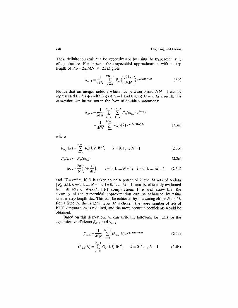
These definite integrals can be approximated by using the trapezoidal ruleof quadrature. For instant, the trapezoidal approximation with a steplength of Aco = 2n/MN to (2.la) gives
Notice that an integer index v which lies between 0 and NM— 1 can berepresented by IM + i with 0 < / < TV — 1 and 0 ^ / ̂ M — 1. As a result, thisexpression can be written in the form of double summations:
where
and w=e}2n'N, If N is taken to be a power of 2, the M sets of TV-data{Fm,,(k),k = Q, 1,..., N- 1}, / = 0, 1,..., M- 1, can be efficiently evaluatedfrom M sets of //-point FFT computations. It is well know that theaccuracy of the trapezoidal approximation can be enhanced by usingsmaller step length Aw. This can be achieved by increasing either N or M.For a fixed N, the larger integer M is chosen, the more number of sets ofFFT computations is required, and the more accurate coefficients would beobtained.
Based on this derivation, we can write the following formulas for theexpansion coefficients fimik and ymtk.
Battle-Lemarie Wavelets 491
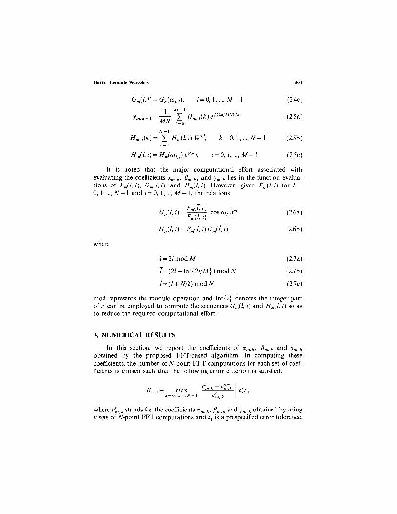
It is noted that the major computational effort associated withevaluating the coefficients ocm,k, /?„,,, and ym,k' lies in the function evalua-tions of Fm(i,l), Gm(l,i), and Hm(l,i). However, given Fm(l,i) for l =0, 1,..., N- 1 and i = 0, 1,..., M- 1, the relations
where
mod represents the modulo operation and Int{r} denotes the integer partof r, can be employed to compute the sequences Gm(l, i) and Hm(l, i) so asto reduce the required computational effort.
3. NUMERICAL RESULTS
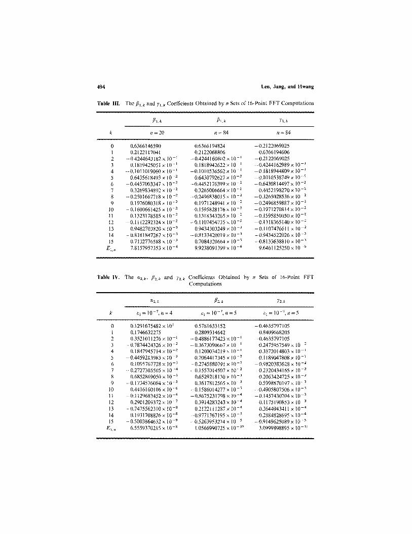
In this section, we report the coefficients of am , k , Pm,k and jm,k
obtained by the proposed FFT-based algorithm. In computing thesecoefficients, the number of Appoint FFT-computations for each set of coef-ficients is chosen such that the following error criterion is satisfied:
where cnmk stands for the coefficients am,k' ftm,k and ym,k obtained by usingn sets of Af-point FFT computations and £: is a prespecified error tolerance.
492 Leu, Jang, and Hwang
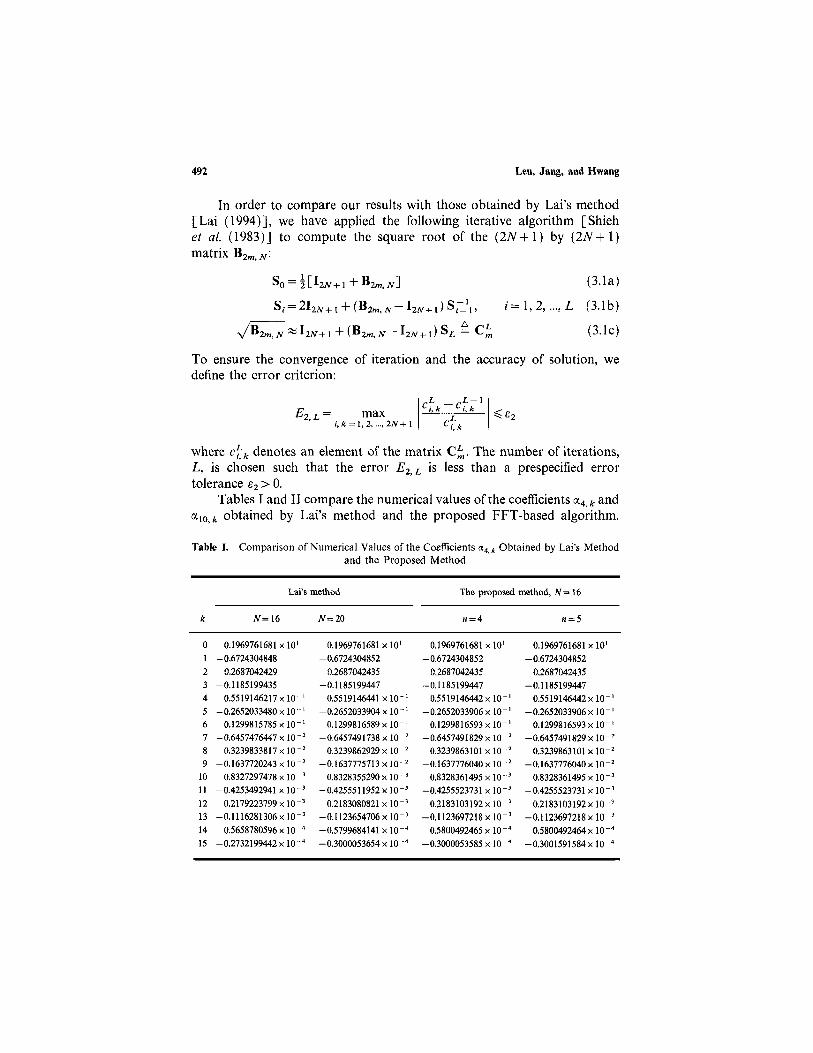
In order to compare our results with those obtained by Lai's method[Lai (1994)], we have applied the following iterative algorithm [Shiehet al. (1983)] to compute the square root of the (2AT+1) by (2N+1)matrix B2m.N:
To ensure the convergence of iteration and the accuracy of solution, wedefine the error criterion:
where c^k denotes an element of the matrix C^. The number of iterations,L, is chosen such that the error E2,L is less than a prespecified errortolerance e2 > 0.
Tables I and II compare the numerical values of the coefficients <x4 ,k anda10,k obtained by Lai's method and the proposed FFT-based algorithm.
Table I. Comparison of Numerical Values of the Coefficients a4,k Obtained by Lai's Methodand the Proposed Method
Lai's method
k
01
3456789
101112131415
N=16
0.1969761681 x 101
-0.6724304848n 026870424200.2087042429
-0.11851994350.5519146217 x 10-1
-0.2652033480 x 10⁻¹
0.1299815785 x 10⁻¹
-0.6457476447 x 10⁻²
0.3239833817 x 10⁻²
-0.1637720243 x 10⁻²
0.8327297478 x 10⁻¹
-0.4253492941 x 10⁻³
0.2179223799 X 10⁻³
-0.1116281306 x 10⁻³
0.5658780596 x 10⁻⁴
-0.2732199442 x 10⁻⁴
N=20
0.1969761681 x 101
-0.67243048520268704242602807042433
-0.11851994470.5519146441 x 10-1
-0.2652033904 x 10⁻¹
0.1299816589 x 10⁻¹
-0.6457491738 x 10⁻²
0.3239862929 x 10⁻²
-0.1637775713 x 10⁻²
0.8328355290 x 10⁻³
-0.4255511952 x 10⁻³
0.2183080821 x 10 -3
-0.1123654706 x 10⁻³
-0.5799684141 x 10⁻⁴
-0.3000053654 x 10⁻⁴
The proposed method, N= 16
« = 4
0.1969761681 x 101
-0.6724304852026870424260.2007042433
-0.11851994470.5519146442 x 10-1
-0.2652033906 x 10⁻¹
0.1299816593 x 10⁻¹
-0.6457491829 x 10⁻²
0.3239863101 x 10⁻²
-0.1637776040 x 10⁻²
0.8328361495 x 10⁻³
-0.4255523731 x 10⁻³
0.2183103192 x 10⁻³
-0.1123697218x10⁻³
0.5800492465 x 10⁻⁴
-0.3000053585 x 10⁻⁴
« = 5
0.1969761681 x 10'-0.6724304852
0.2687042433-0.1185199447
0.5519146442 x 10⁻¹
-0.2652033906 x 10⁻¹
0.1299816593 x 10⁻¹
-0.6457491829 x 10⁻¹
0.3239863101 x 10⁻²
-0.1637776040 x 10⁻²
0.8328361495 x 10⁻³
-0.4255523731 x 10⁻³
0.2183103192 x 10⁻³
-0.1123697218 x 10⁻³
0.5800492464 x 10⁻⁴
-0.3001591584 x 10⁻⁴
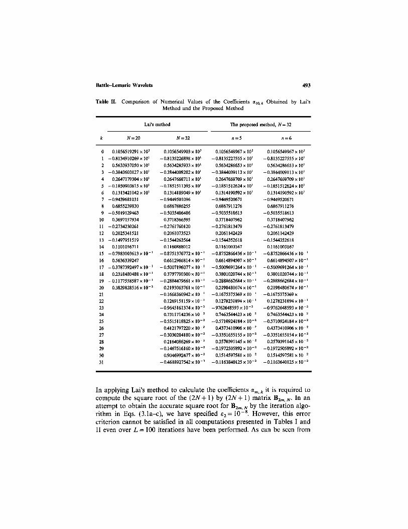
Battle-Lemarie Wavelets 493
Table II. Comparison of Numerical Values of the Coefficients a10i/t Obtained by Lai'sMethod and the Proposed Method
Lai's method
k
01234567S9
101112131415
16171819202122232425262728293031
N=20
0.1056519291 x 10²
-0.8134910269x101
0.5633937050x10'-0.3843603127 x 10'
0.2647179304x10'-0.1850903815 x 10'
0.1313421042x10'-0.9439681031
0.6855239830-0.5019129463
0.3697157934-0.2734230261
0.2025341521-0.1497951519
0.1101056711-0.7983003613x10-'
0.5636339247-0.3787392497x10-'
0.2318480488x10-'
-0.1177558587x10-'
0.3829828516 x10 - 2
N=32
0.1056549903 x 10²
-0.8135226898x10'0.5634285933x10'
-0.3844008282x10'0.2647668711x10'
-0.1851511395x10'0.1314189049x10'
-0.94495010960.6867886255
-0.50354864860.3718366595
-0.27617601200.2061073523
-0.15442635640.1160888012
-0.8751376772x10-'0.6612966814x10-'
-0.5007196077x10-'
0.3797790300x10-'
-0.2884479661x10-'
0.2193063761x10-'
-0.1668360942x10-'
0.1269151159x10-'
-0.9645161374 x 10⁻²
0.7311714236xl0-2
-0.5515118825 x 1 0 - 2
0.4121797220 x l 0 - 2
-0.3030284180 x10 - 2
0.2164086269 x 10⁻²
-0.1467516160 x 10⁻²
0.9046992477 x 10⁻²
-0.4618927542 x l 0 - 3
The proposed method, N=32
n = 5
0.1056549967 xl02
-0.8135227555x10'0.5634286653x10'
-0.3844009113x10'0.2647669709x10'
-0.1851512624x10'0.1314190592x10'
-0.94495206710.6867911276
-0.50355186130.3718407962
-0.27618134790.2061142429
-0.15443526180.1161003167
-0.8752866436x10-'0.6614894507x10-'
-0.5009691264x10-'0.3801020744x10-'
-0.2888662684x10-'0.2198480674x10-'
-0.1675375369x10-'0.1278231894x10-'
-9762648593 xl0-2
0.7463544423 x 10- 2
-0.5710924184 x 10⁻²
0.4373410906 x 10⁻¹
-0.3351655155 x l 0 - 2
0.2570391145 x l 0 - 2
-0.1972505892 x l 0 - 2
0.1514597581 x 10⁻²
-0.1163840125 xl0-2
n = 6
0.1056549967 x 10²
-0.8135227555 x 10'0.5634286653 x 10'
-0.3844009113x10'0.2647669709 x 10'
-0.1851512624x10'0.1314190592x10'
-0.94495206710.6867911276
-0.50355186130.3718407962
-0.27618134790.2061142429
-0.15443526180.1161003167
-0.8752866436x10"'0.6614894507x10-'
-0.5009691264x10-'
0.3801020744x10-'
-0.2888662684x10-'
0.2198480674x10-'
-0.1675375369 x0.1278231894x10-'
-0.9762648593 x 10 -2
0.7463544423 x 10⁻²
-0.5710924184 xl0-2
0.4373410906 x l 0 - 2
-0.3351655154xl0-2
0.2570391145 xl0-2
-0.1972505892 x l 0 - 2
0.1514597581 x 10- 2
-0.1163640125 x l0-2
In applying Lai's method to calculate the coefficients am..k it is required tocompute the square root of the (2N + 1) by (2N+ 1) matrix B2m,N. In anattempt to obtain the accurate square root for B2m, N by the iteration algo-rithm in Eqs. (3.1a-c), we have specified £ 2 =10 - 8 . However, this errorcriterion cannot be satisfied in all computations presented in Tables I andII even over L= 100 iterations have been performed. As can be seen from
494 Leu, Jang, and Hwang
Table HI. The B1,k and yl,k Coefficients Obtained by n Sets of 16-Point FFT Computations
k
0123456789
101112131415
E1, n
B1,k
n = 20
0.63661465900.2122117041
-0.4244643 1 82 x 10-1
0.1819425051 x 10⁻¹
-0.101 1019060 x10-1
0.6435618493 x 10- 2
- 0.4457003347 x 10 - 2
0.3269834892 x 10 - 2
-0.2501667718X10⁻²
0. 1976080318 x 10 - 2
-0.1 600661 425 x10-2
0.1 323178585 x 10-2
-0.11 12292324 x l0-2
0,9482703820 x10⁻³
- 0.8181847267 x 10- 3
0.7132776588 x 10⁻³
7.8157957353 x 10⁻⁴
Bl.k
n = 84
0.63661948240.2122068806
-0.4244160802x10⁻¹
0.1818942622x10⁻¹
-0.1010536562x10⁻¹
0.6430792627 x 10⁻²
-0.44521 76399 x 10-2
0.3265006664 x 1 0 - 2
-0.249683801 5 x10⁻²
0.1971248941 x 10⁻²
-0.1595828176 xl0 - 2
0.1318343265 x 10 - 2
-0,1107454735 x 10⁻²
0,9434303249 x 10⁻³
-0.8133420019 x 10 - 3
0.7084320664 x 1 0 - 3
9.9238091 399 x 10 - 6
y1,k
n-84
-0.21220690250.6366194606
-0.2122069025-0.42441 62989 x 10 - 1
-0.1818944809x10⁻¹
- 0,1 01 0538749 x 10-1
-0.64308 14497 x 10-2
-0.4452198270 x 10⁻²
-0.3265028536 x 10⁻²
- 0.2496859887 x 1 0 - 2
- 0.1971270814 x 10⁻²
-0.1595850050 x 10⁻²
-0.1318365140 x 10⁻²
-0.1107476611 x 10⁻²
- 0.9434522026 x 10⁻³
-0.8133638810 x 10⁻³
9.6461 125250 x l0-6
Table IV. The x2,K, B2,K and y2,K Coefficients Obtained by n Sets of 16-Point FFTComputations
k
0123456789101112131415E1.n
a2,k
£1 = 10-7,n= 4
0.1291675482x101-0.17466322750.3521011276 x 10-1
- 0.7874424326 x 10-20.1 847945714x10-2
-0.4459213983xl0-30.1095767728xl0-3
-0.2727305505x10-40.6852869050 x 10-5
-0.1734576084 x 10-50.4416160106 x10-6
-0.1129683452 xl0-60.2901209372 x 10⁻⁷
- 0.7475562310x10-80.1931708826 x l0-8
-0.5003864632x10-96.5559370215x10-8
B2,K
E1=10-7,n = 5
0.57816331520.2809314642
-0.4886177423 x 10⁻¹- 0.3673090667 x 10-10.1200034219 x 10-10.7064417345 x 10⁻²
-0.2745880791 x 10⁻²-0.1557014507 x l0-20.6529218130 x l 0 - 3
0.3617812565 x 10⁻³- 0.1 586014277 x 10-3-0.8675231798 x 10-40.3914283243 x l0-40.2122111287x10⁻⁴
-0.9771367195 xl0-5
-0.526395 3274 x 10-51. 0566990725 x 10-10
Y2,k
£, = 10-7,n = 5
-0.46357975050.8409668205
-0.46357971050.2475957549 x l0-20.3872014803 x 10-10.1189047808x10-1
- 0.9820383628 x 10⁻²-0.2320434165 xl0-2
0.2063424725 x 10⁻²
0.5998870197 x 10⁻³
- 0.4905807506 x 10⁻³
-0.1457430704 x 10-30.1175190853 x 10-30.3644943411 x 10⁻⁴
- 0.2884828695 x 10⁻⁴-0.91 49625089 x 10-53.0999898895x10⁻¹¹
Battle-Lemarie Wavelets 495
Table V. The a3,k, B3i/! and y3tk Coefficients Obtained by n Sets of 16-Point FFTComputations
k
0123456789
101112131415
£1.n
a3,k
E1, = 10-7,n = 4
0.1585523561 x 101
-0.38330741430.1224100849
-0.4375513105x10⁻¹
0.1647263704x10⁻¹
-0.6383677845 x 10⁻²
0.252015991 I x l O " 2
-0.1007864710 x 10⁻²
0.4069368596 xl0-3
-0.1655186609 xl0-3
0.6771792342x10⁻³
-0.2783708099 x 10⁻⁴
0.1148828713x10⁻⁴
-0.4756961450 xl0-5
0.1975316885 xl0-5
-0.8222607034 x 10⁻⁶
7.9051945568 xl0-2
B3,k
E1 = 10-7 , n= 5
0.55442677210.2992858005
-0.4209818666x10⁻¹
-0.6351 332389 x10-1
0.2071587309x10⁻¹
0.1915847781 x 10⁻¹
-0.8169337725 x 10⁻²
-0.66983701 19 x 10-2
0.3232076854 x 10⁻²
0.2460993465 xl0-2
-0.1266439398 x 10⁻²
-0.9514526370 xl0-3
0.5 126696849 x 10-3
0.3679246870 xl0-3
-0.2033151 140 xl0-3
-0.1488409691 x 10⁻³
9.1476443013 x 10⁻⁸
y3,k
E1, = 10- 7 ,n=15
-0.69820393110.1 093504740 x 10-1
-0.69820393110.10676360300.4157237841 x 10-1
0.3344218155 x 10⁻¹
-0.3408059105x10⁻¹
-0.5051 746849 x l 0 - 2
0.8917848757 x 10⁻²
0.3554291 285 x 10-2
-0.3865855446 xl0-2
-0.1 198514983 x 10-2
0.1 407777305 x 10-2
0.5323656132 x 10⁻³
-0.5646593665 xl0-3
- 0.2070307864 x 10⁻³
9.1 830624272 x 10-8
Table VI. The a4,k B4,k and y4,k Coefficients Obtained by n Sets of 16-Point FFTComputations
k
01234567
89101112131415
E1,n
a4,k
E1 =10-7,n=5
0.1969761681 x 101
-0.67243048520.2687042435
-0.11851994470.5519146442x10-1
-0.2652033906x10⁻¹
0.1299816593x10⁻¹
-0.6457491829 x l0 - 2
0.3239863101 xl0- 2
-0.1637776040 xl0-2
0.8328361495 x l 0 - 3
-0.4255523731 xl0- 3
0.2183103192 x 10⁻³
-0.1 123697218 xl0-3
0.5800492464x10⁻⁴
-0.3001591584x10⁻⁴
3.2848862830x10⁻¹⁰
B4,k
£1 = 10-7,n = 6
0.54173575620.3068296367
-0.3549797994x10⁻¹
—0.77807921 88 x 10-1
0.2268462014x10⁻¹
0.2974681657x10⁻¹
-0.1214548916x10⁻¹
-0.1271542110x10⁻¹
0.6141430858 xl0-2
0.5799320148 xl0-2
-0.3078629404 x 10⁻²
-0.2745289232 x 10⁻²
0.1546239145 xl0-2
0.1 330869377 x 10-2
-0.78046191 18 x10-3
-0.6556285102 xl0-3
7.3740844711 x 10⁻³
Y4,k
£1 = 10-7,n = 6
-0.1 002605289 x 101
0.1445867055 x 101
-0.1002605289x101
0.2711395073-0.6035702811xl0-2
0.7204433308x10⁻¹
-0.7295624620x10⁻¹
0.1509181419xl0-2
0.1417196409x10⁻¹
0.9574629656 x 10⁻²
-0.1123099156x10⁻¹
-0.248245 1693 xl0-2
0.4165162504 x 10⁻²
0.1926453123 xl0-2
-0.2352521366 xl0-2
4.9610276836 x 10⁻⁸

496 Leu, Jang, and Hwang
Table VII. The a5,k B0S,k and y5,k Coefficients Obtained by n Sets of 16-Point FFTComputations
k
0123456789
101112131415
El,n
a5,k
E1 = 10-7,n = 5
0.2491669496x101
-0,1082988900 x 101
0.5027657851-0.2517361591
0.1325747036-0,7210191 165x10-1
0.4004660171 x 10⁻¹
-0.2256556088x10⁻¹
0.1284815080x10⁻¹
-0.7372878336x10⁻²
0.4256887545 xl0-2
-0.2469937034 x10⁻²
0.1438929965 x 10⁻²
-0.8411411096x10⁻³
0.493121 1630 x l0-3
-0.28981 47067 x 10-3
2.5017791331 x 10⁻⁸
B5,k
£1 = 10-7,n =7
0.53380277270.3106624020
-0.3025077218x10⁻¹
-0.8616864485x10⁻¹
0.22 17556695x10-1
0.3763896929x10⁻¹
-0.1414773187x10⁻¹
-0.1829658245x10⁻¹
0.8427867294 x 10⁻²
0.9429453951 x 10⁻²
-0.4902168775 x 10⁻²
-0.504451 9293 x 10-2
0.28331 17227 x 10-2
0.2766502972 x 10⁻²
-0.1637536752 x 10⁻²
-0.1543382979 xl0-2
2.9192828047 x 10⁻⁸
Y5,k
E1= 1 0 - 7
-0.1424958449x101
0.1938794625 x 101
-0.1424958449x10'0.5234743831
-0.11727717300.1459949400
-0.13583894570.2680900253x10-1
0.9797776263 x 10⁻²
0.2190067561x10⁻¹
-0.2448179960x10⁻¹
-0.1 367760800 x 10-2
0.6823498335 x 10⁻²
0.4814843009 x 10⁻²
-0.5986553810 x 10⁻²
- 0.1505958822 x 10⁻²
2.9929937685x10-*
Table VIII. The a6,k B6,k and y6,k Coefficients Obtained by n Sets of 16-Point FFTComputations
k
0123456789
101112131415
E1.n
a6,k
E1 = 10-7,n= 6
0.3212528821 x 101
-0.1671293234x101
0.8693742694-0.4762545765
0.2724067238-0.1606709064
0.9681281005x10⁻¹
-0.5922120471 x 10⁻¹
0.3662546372x10⁻¹
- 0.2283852709 x 10⁻¹
0.1433277889x10⁻¹
-0.9040851 847 x 10-2
0.5726641232 x l0-2
- 0.3639994948 x 10⁻²
0.2320497824 x 10 -2
0.1483066330 x l0-2
5.04122429746 x 10⁻¹⁰
B6,k
E1 = 10-7,
0.52837404860.3128686248
-0.2617712270x10⁻¹
-0.9140675148x10⁻¹
0.2084141731 xl0-1
0.4335443698x10⁻¹
-0,1485366292x10⁻¹
-0.2299510826x10-'0.99063503 14 x 10-2
0.1287541406x10⁻¹
-0.6398863214 x 10⁻²
-0,7468483203 x 10⁻²
0.4078823935 x 10⁻²
0,4440019274 xl0-2
-0.2588158265 x l0-2
-0.2686458518 xl0-2
4.4662881 897 x 10-7
Y6,k
E1 = 10-7,n= 8
-0.2023716476=101
0.2631371143x101
-0.2023716476x101
0.9087204939-0.3221971445
0.2806034087-0.2405573335
0.8355739345 x 10⁻¹
-0.1484692573x10⁻¹
0.4752244539x10⁻¹
-0.4842008833x10⁻¹
0.6591930069 x 10⁻²
0.60811 17846 x 10-2
0.1093068653x10⁻¹
-0.1274276488x10⁻¹
- 0.1094039730 x 10⁻²
4.25869561 15 x 10-8
Battle-Lemarie Wavelets 497
Table IX. The a7,k, B7,k and y7,k Coefficients Obtained by n Sets of 16-Point FFTComputations
k
0123456789
101112131415
£i.n
a7,k
E1 =10-7,n = 6
0.4220011920x101
-0.2519132940x101
0.1436129545x101
-0.84382974460.5131720148
-0.32084387870.2047872654
-0.13271818620.8699307801 x 10-1
-0.5751475781 x 10⁻¹
0.3828074201 x 10⁻¹
-0.2561494897x10⁻¹
0.1721418703-0.1161015239x10⁻¹
0.7854219903 x 10⁻²
-0.53271 10257 x 10-2
9.9106247190 x 10⁻⁹
B7,k
E1 = 10-7,n = 9
0.52443129920.3142494062
-0.2298578799x10⁻¹
-0.9487124506x10⁻¹
0.1931162232x10-0.4751360833x10-
-0.1283080077x10⁻¹
-0.2680051269x10⁻¹
0.1072202268x10⁻¹
0.1594167442x10⁻¹
-0.7486602769 x 10⁻²
-0.9803534057 x 10⁻²
0.5135017984xl0-2
0.6173068053 x 10⁻²
-0.3492708598 x l0-2
-0.3955477082 x 10⁻²
8.9467457402xl0-9
Y7,k
E1 = 10-7,n = 9
-0.2881512458x101
0.3610237726 x 101
-0.2881512458x101
0.1494781035x101
-0.67115807060.5149401970
-0.41628403920.1927909029
-0.7621064084x10⁻¹
0.9885255586x10⁻¹
-0.9219851716x10⁻¹
0.2883013387x10⁻¹
-0.3821388975 x10⁻²
0.2418003593x10⁻¹
-0.2554001460x10⁻¹
0.2900228661 x 10⁻²
1.6440330405 x l0-8
Table X. The a8,k B8,k and y8,k Coefficients Obtained by n Sets of 16-Point FFTComputations
k
0123456789
101112131415
El.n
a8,k
EI = 10-7,n = 6
0.564(792173 x 101
-0.3746W3949 x 101
0.2304631219 x 101
-0.14341566341 x 101
0.916015118157-0.5990201950
0.3992998709-0.2701564790
0.1848824865-0.1276491139
0.887471 3004 x 10-1
-0.6204356370 x 101
0.4357061944x10⁻¹
-0.3071186187x10⁻¹
0.2171575655x10⁻¹
-0.1539568396x10⁻¹
9.1526065680 x 10⁻⁸
B8,k
E1= 10-7,n= 9
0.52144179800.3151681650
-0.2044369189x10⁻¹
-0.9726595592x10⁻¹
0.1782266320x10⁻¹
0.5058711547x10⁻¹
-0.1442925549x10⁻¹
-0.2984267354x10⁻¹
0.1107049042x10⁻¹
0.1858223268x10⁻¹
-0.8204151392 x l0-2
-0.1194804287x10⁻¹
0.5957370954 x 10⁻²
0.7857778585 x 10⁻²
- 0.4277763532 x 10⁻²
-0.5256051921 x 10⁻²
7.7592031489 x 10⁻⁸
Y8,k
E1= 10-7,n = 9
-0.4118882910x101
0.5002466701 x 101
-0.4118882910x101
0.2383541834x101
-0.1243498182x101
0.9103832872-0.7099010602
0.3895514128-0.2013127237
0.1969221774-0.1719501984
0.7805884517x10⁻¹
-0.3288650044x10⁻¹
0.5210296102x10⁻¹
-0.5021436082x10⁻¹
0.1522532735x10⁻¹
4.0210724605 x 10⁻⁸
498 Leu, Jang, and Hwang
Table XI. The a9,k B9,k and y9,k Coefficients Obtained by n Sets of 32-Point FFTComputations
k
0123456789
10111213141516171819202122232425262728293031
£1,n
a9,k
E1= 10-7,n = 5
0.7665064235 x 101
-0.553 11 44352 x101
0.3627527947x101
-0.2371661359x101
0.1577338035x101
-0.1 069689069 x 101
0.7380015428-0.5163753957
0.3653795450-0.2608472865
0.1875462057-0.1356159273
0.9852275792 x 10⁻¹
-0.7185151476x10⁻¹
0.5257005864 x 10⁻¹
-0.3856851274x10⁻¹
0.2836298733x10⁻¹
-0.2090073267x10⁻¹
0.1542951999x10⁻¹
- 0.11 40866585 x 10-1
0.844761 2925 x 10-2
-0.6263063542 x l0-2
0.4648787298 x 10⁻²
-0.34541 92668 x 10-2
0.2569020942 x 10⁻²
-0.1912353745 x 10⁻²
0. 1424681 780 x 10-2
-0.1062159395 x 10⁻²
0.7924280959 xl0-3
-0.5915713389 x 10⁻³
0.4418882313 x 10⁻³
-0.3302620523 x l0-3
7.5042505290x10⁻⁹
B9,k
E1 = 10-7, n = 7
0.51909924850.3158090460
- 0.1 838291 073 x 10-1
- 0.9898265673 x 10⁻¹
0.1645594974x10⁻¹
0.5290021014x10⁻¹
-0.1384780212x10⁻¹
-0.3227218819x10⁻¹
0.1 11 1269034 x 10-1
0.2081 988269 x 10-1
-0.8627205895 x l0-2
-0.1 386499436 x 10-1
0.6555903540 x 10⁻²
0.9436378605 x 10⁻²
-0.4917361545 x 10⁻²
- 0.6527985768 x 10⁻²
0.3660490033 x 10⁻²
0.4573855104 x 10⁻²
-0.2713563055 xl0-2
-0.3237254992 x 10⁻²
0.20074631 90 x 10-2
0.2309939388 x 10⁻²
-0.1483941 143 x 10-2
-0.1659173932 xl0-2
0.1096930456 x 10⁻²
0.1198229741 x 10⁻²
-0.8 11 2023767 x 10-3
- 0.8692570039 x 10⁻³
0.6003 11 2028 x 10-3
0.6330023874 x 10⁻³
— 0.4446086064 x 10⁻³
- 0.4624509995 x 10⁻³
7.0555457938 x 10⁻⁹
Y9,k
E1 = 10-7, n = 7
-0.591 3364927 x 101
0.6994841487 x 101
-0.591 3364927 x 10'0.3727905351 x 10'
-0.2161951004x10'0.1563251503x10'
-0.1196273535x10'0.7313385642
-0.43483486880.3769150758
-0.31528377970.1760925772
-0.9846193386 x 10⁻¹
0.1083633829-0.9760633914x10⁻¹
0.4462946743 x 10⁻¹
-0.2050330969x10-'0.3456453174x10-'
-0.3369176341x10-'0.1067514532 x 101
-0.2282593219 xl0-2
0.1205258678x10⁻¹
- 0.1 281 540499 x 10-1
0.1933575054 x l0-2
0.1275025405 xl0-2
0.4605727938 x 10⁻²
- 0.5340846649 x 10⁻²
-0.9929347378 x 10⁻⁴
0.1432731027 x 10⁻²
0. 1931 094705 x 10-2
-0.2412961369 xl0-2
-0.4082130601 x 10⁻³
3.2439016323 xl0-8
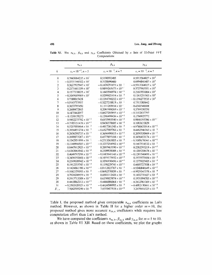
Table I, the proposed method gives comparable &4,k coefficients as Lai'smethod. However, as shown in Table II for a higher order m=10, theproposed method gives more accurate &10,k coefficients while requires lesscomputation effort than Lai's method.
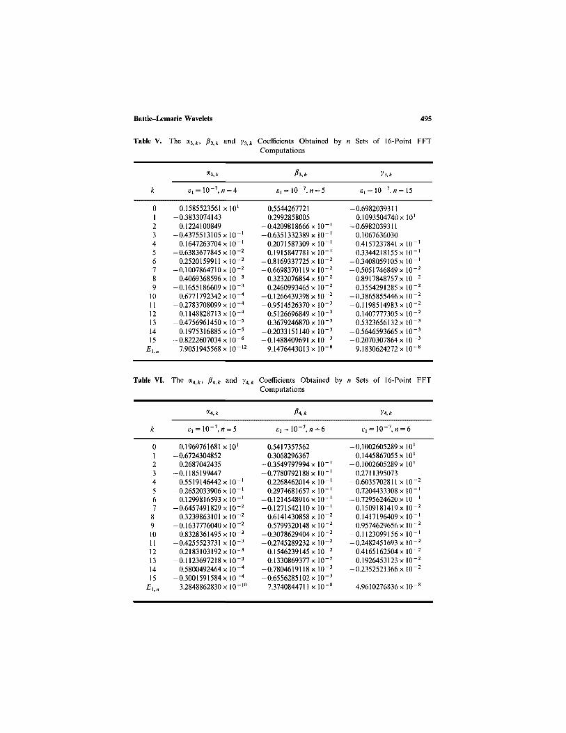
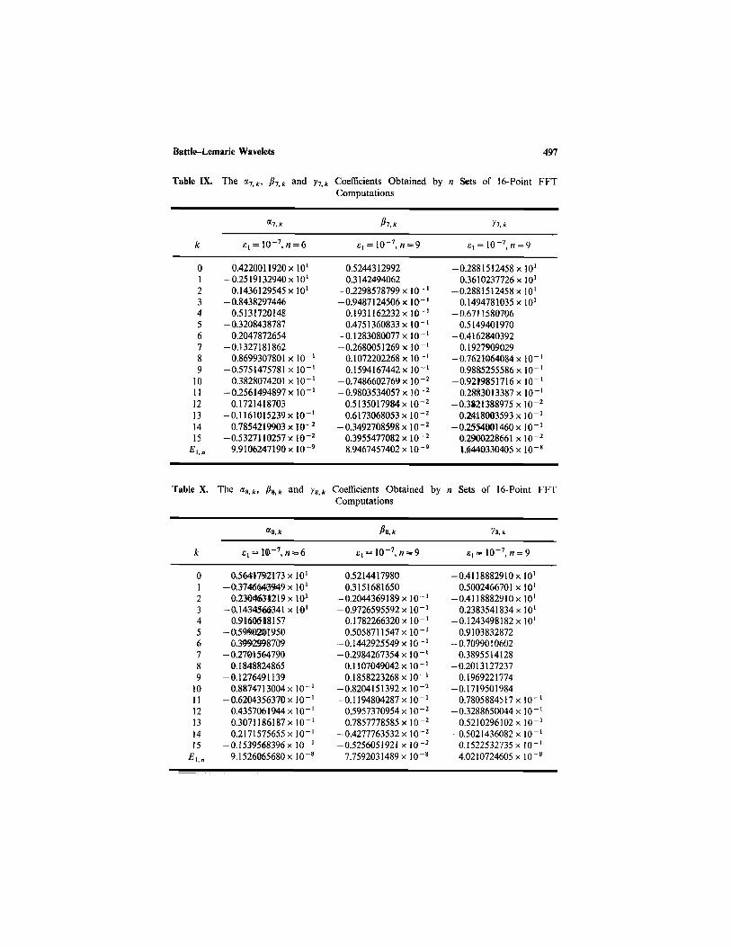
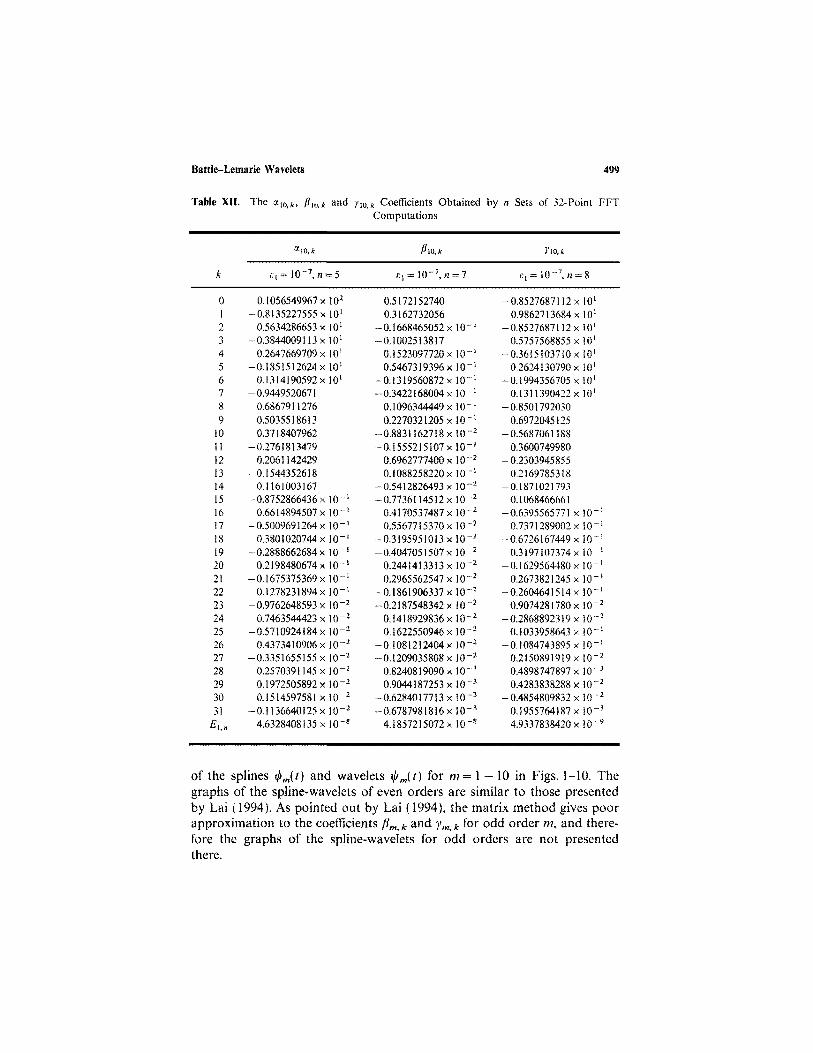
We have computed the coefficients am,k Bm,k and ym,k for m=1 to 10,as shown in Table III-XII. Based on these coefficients, we plot the graphs
Battle-Lemarie Wavelets 499
Table XII. The oc,M, llw,k and yw_k Coefficients Obtained by n Sets of 32-Point FFTComputations
k
0123456789
10111213141516171819202122232425262728293031
£i..
a)0,*
«, = 10-7,n = 5
O.I 056549967 x102
-0,8135227555x10'0,5634286653x10'
-0,38440091 13 x 10'0.2647669709x10'
-0.1851512624x10'0.1314190592 x 10'
-0.94495206710.6867911276
-0.50355186130.3718407962
-0.27618134790,2061 142429
-0.15443526180.1161003167
- 0.8752866436 x 10~'0.661 4894507 x 10"'
-0.5009691264x10-'0.3801020744x10-'
- 0.2888662684 x 10 -'0.2198480674x10-'
-0.1675375369x10-'0.1278231894x10-'
-0.9762648593 x 10 -2
0.7463544423 x lO ' 2
-0,5710924184 x I0~2
0.4373410906 x 10~2
-0.3351655155 x 10~2
0.2570391 145 x 1Q-2
-0.1972505892 x lO- 2
0.1514597581 x 10~2
-0.1136640125 x 10~2
4.6328408 135 x 10 -8
ft\0,k
B, = 10-7,« = 7
0.51721527400.3162732056
- 0.1668465052 x 10 -'-0.1002513817
0.1523097720x10-'0.5467319396x10-'
-0.1319560872x10^'-0.3422168004x10"'
0.1 096344449 x 10 ~'0.227032 1205 x 10 "'
-0.8831 162718 x tO"2
-0.1555215107x10-'0.6962777400 x 10"2
0.1088258220x10-'-0.541 2826493 x 10"2
-0.77361 14512 x 10~2
0.41 70537487 x 10 ~2
0.5567715370xlO"2
-0.3195951013 x 10~2
-0.4047051507 x 10~2
0.2441413313 x l O - 2
0.2965562547 x 10 ~2
-0.1861906337 x 10 -2
-0.2187548342 x 10 -2
0.1418929836 x 10"2
0, 1622550946 x 10 -2
-0.1081212404 x lO- 2
-0.1209035808 x 10 -2
0.824081 9090 x 10~3
0.9044187253 x 10 ~3
-0.6284017713 x lO- 3
-0.6787981816x10-'4.1857215072 xlO" s
)'io,<s
,;,= 10-',« = 8
-0.8527687112x10'0.9862713684x10'
-0.85276871 12 x 10'0.5757568855x10'
-0.3615103710x10'0.2624130790x10'
-0.1 994356705 x 10'0.1311390422 x 10'
-0.85017920300.6972045125
-0.56870611880.3600749980
-0.23039458550.2169785318
-0.18710217930.1068466661
-0.6395565771 x 10~'0.7371 289002 x 10~'
-0.6726167449x10-'0.3197107374 x IQ~1
-0.1 629564480 x 10~'0.2673821245x10-'
-0.2604641 5 14 x ]0~ '0.9074281 780 x 10 -2
-0.286889231 9 x 10"2
0.1033958643x10-'-0.1084743895x10-'
0.2150891919 x l O - 2
0.4898747897 x 10 -3
0.4283838288 x 10~2
- 0.4854809832 x 1Q-2
0.1955764187 x lO"3
4.9337838420 x 10~9
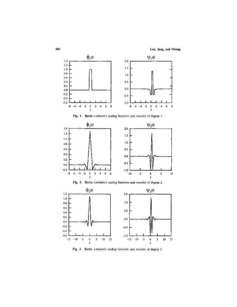
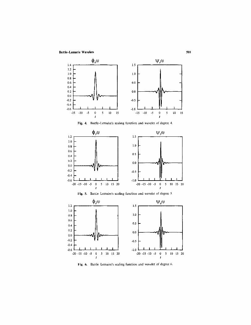
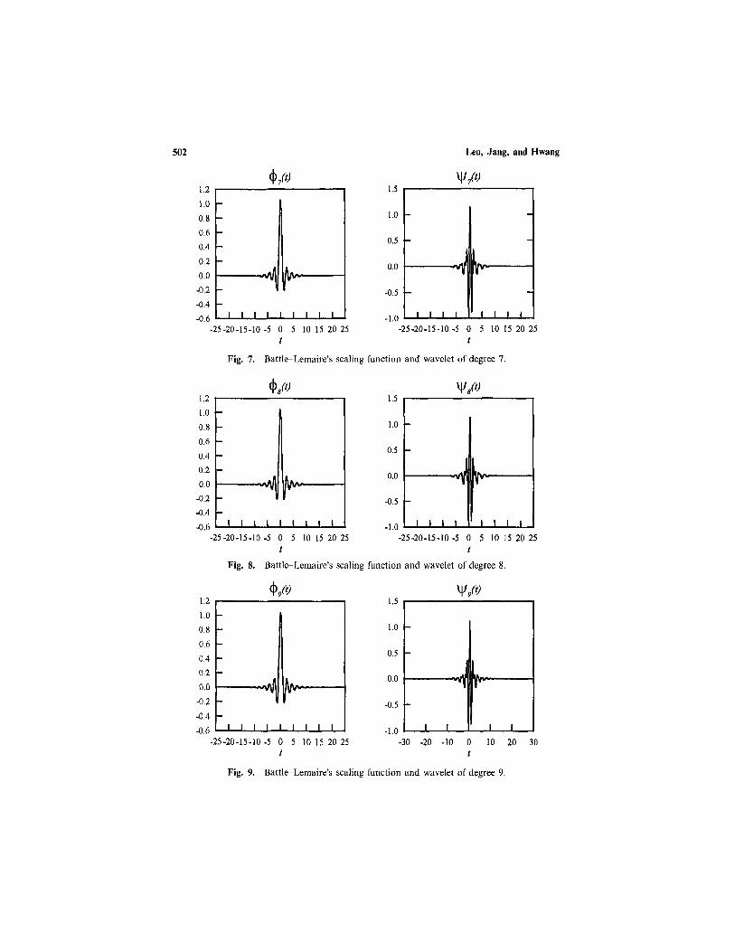
of the splines O m ( t ) and wavelets W m ( t ) for m =1 — 10 in Figs. 1-10. Thegraphs of the spline-wavelets of even orders are similar to those presentedby Lai (1994). As pointed out by Lai (1994), the matrix method gives poorapproximation to the coefficients m, k and ym, k for odd order m, and there-fore the graphs of the spline-wavelets for odd orders are not presentedthere.
500 Leu, Jang, and Hwang
Fig. 1. Battle-Lemaire's scaling function and wavelet of degree 1.
Fig. 2. Battle-Lemaire's scaling function and wavelet of degree 2.
Fig. 3. Battle-Lemaire's scaling function and wavelet of degree 3.
Battle-Lemarie Wavelets 501
Fig. 4. Battle-Lemaire's scaling function and wavelet of degree 4.
Fig. 5. Battle-Lemaire's scaling function and wavelet of degree 5.
Fig. 6. Battle-Lemaire's scaling function and wavelet of degree 6.
502 Leu, Jang, and Hwang
Fig. 7. Battle-Lemaire's scaling function and wavelet of degree 7.
Fig. 9. Battle-Lemaire's scaling function and wavelet of degree 9.
Battle-Lemane Wavelets 503
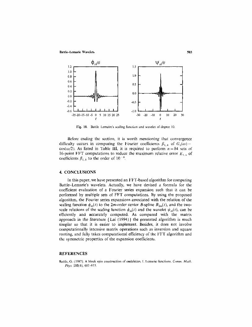
Fig. 10. Battle-Lemaire's scaling function and wavelet of degree 10.
Before ending the section, it is worth mentioning that convergencedifficulty occurs in computing the Fourier coefficients Bl,k of G,(co) =cos(w/2). As listed in Table III, it is required to perform n = 84 sets of16-point FFT computations to reduce the maximum relative error E1,„ ofcoefficients Bl,k to the order of 10- 6 .
4. CONCLUSIONS
In this paper, we have presented an FFT-based algorithm for computingBattle-Lemarie's wavelets. Actually, we have devised a formula for thecoefficient evaluation of a Fourier series expansion such that it can beperformed by multiple sets of FFT computations. By using the proposedalgorithm, the Fourier series expansions associated with the relation of thescaling function O m ( t ) to the 2m-order center B-spline B2m(t), and the two-scale relations of the scaling function O m ( t ) and the waveletWm(t), can beefficiently and accurately computed. As compared with the matrixapproach in the literature [Lai (1994)] the presented algorithm is muchsimpler so that it is easier to implement. Besides, it does not involvecomputationally intensive matrix operations such as inversion and squarerooting, and fully takes computational efficiency of the FFT algorithm andthe symmetric properties of the expansion coefficients.
REFERENCES
Battle, G. (1987). A block spin construction of ondelettes. 1. Lemarie functions. Comm. Math.Phys. 110(4), 601—615.
504 Leu, Jang, and Hwang
Chui, C. K. (1992). An Introduction to Wavelets, Academic Press, Boston, Massachusetts.Daubechies, I. (1992). Ten Lectures on Wavelets, CBMS Series 61, SIAM, Philadelphia,
Pennsylvania.Lai, M. J. (1994). On the computation of Battle-Lemarie's wavelets. Math. Comput. 63(208),
689-699.Lancaster, P., and Tismenetsky, M. (1985). The Theory of Matrices, Second Edition,
Academic Press, Orlando Florida.Lemarie, P. G. (1988). Ondelettes with exponential localization. J. Math. Pures Appl.
Neuvieme Serie, 67(3), 227-236.Shieh, L. S., Tsay, Y. T., and Yates, R. E. (1983). Some properties of matrix sign functions
derived from continued fractions. IEE Proc.-D: Control Theory Appl. 130(3), 111-118.
Printed in Belgium


