Journal of Hydraulic Research Vol. 41, No. 2 (2003), pp. 115–125

© 2003 International Association of Hydraulic Engineering and Research

A multiphase oil spill model

Un modèle multiphase de nappe d’huilePAVLO TKALICH, Senior Research Fellow, Tropical Marine Science Institute, National University of Singapore, Singapore 119223

MD. KAMRUL HUDA, Project Executive, Applied Research Corporation, National University of Singapore, Singapore 119260

KARINA YEW HOONG GIN, Assistant Professor, School of Civil and Environmental Engineering,Nanyang Technological University, Singapore 639798

ABSTRACTA multiphase oil spill model has been developed to simulate consequences of accidental oil spills in the marine environment. Six state variables arecomputed simultaneously: an oil slick thickness on the water surface; concentration of dissolved, emulsified and particulate oil phases in the watercolumn; and concentration of dissolved and particulate oil phases in the bottom sediments. A consistent Eulerian approach is applied across the model,the oil slick thickness is computed using the layer-averaged Navier–Stokes equations, and for transport of the oil phases in the water column theadvection–diffusion equation is employed. The kinetic terms are developed to control the oil mass exchange between the variables. The governingequations are verified using test cases, data and other models. The model is useful for short and long-term predictions of the spilled oil dynamics andfate, including application of the oil combating elements, such as chemical dispersants and booms.

RÉSUMÉUn modèle multiphase de nappe d’huile a été développé pour simuler les conséquences des déversements accidentels d’huile dans l’environnementmarin. Six variables d’état sont calculées simultanément: une épaisseur de nappe d’huile sur la surface de l’eau; la concentration des phases dissoutes,émulsionnées et particulaires de l’huile dans la colonne d’eau; et la concentration des phases dissoutes et particulaires d’huile dans les sédimentsdu fond. Une approche Eulérienne consistante est appliquée à l’ensemble du modèle: l’épaisseur de la nappe d’huile est calculée en utilisant leséquations de Navier-Stokes moyennées sur la couche de surface, pour le transport des phases d’huile dans la colonne d’eau, on utilise une équation deconvection-diffusion. Les termes cinétiques sont développés de manière à contrôler les échanges de masse d’huile entre les variables. Les équationssont vérifiées en utilisant des cas tests, des données, et d’autres modèles. Le modèle est utile pour les prévisions à court et à long terme de la dynamiqueet de l’évolution des déversements d’huile, en tenant compte des mesures défensives telles que les dispersants chimiques et les barrages flottants.

Keywords: oil spill model; high-order numerical scheme; spill combating techniques; Singapore Strait.

1 Introduction

Rapid economic growth has caused a significant increase infossil fuel consumption in recent decades. The world produc-tion of crude oil is about 3 billion tons per year and half ofit is transported by sea (Clark, 1992). A significant amount ofoil is spilled into the sea from operational discharges of shipsas well as from accidental tanker collisions and grounding. Oilspills resulting from tanker traffic, offshore drilling, and associ-ated activities are likely to increase in years to come as demandfor petroleum and petroleum products continues to rise. Beingstrategically positioned between the Indian and Pacific Oceans,the Singapore Strait has been extensively used by international

Revision received August 31, 2002. Open for discussion till August 31, 2003.

115

maritime traffic. Oil shipping and refinement are crucial indus-tries for the Singapore economy, but are also potential threatsto the coastal marine environment. An example of this is the oilspill on October 15, 1997, caused by the collision of two tankers,the “Evoikos” and “Orapin Global”, when approximately 28,000tons of marine fuel oil was accidentally discharged into the Strait.

The transport and fate of spilled oil in water bodies aregoverned by physical, chemical, and biological processes thatdepend on the oil properties, hydrodynamics, meteorologicaland environmental conditions. The processes include advection,turbulent diffusion, surface spreading, evaporation, dissolution,emulsification, hydrolysis, photo-oxidation, biodegradation andparticulation. When liquid oil is spilled on the sea surface,

116 Pavlo Tkalich et al.

it spreads to form a thin film – an oil slick. The movement of theslick is governed by the advection and turbulent diffusion due tocurrent and wind action. The slick spreads over the water sur-face due to a balance between gravitational, inertial, viscous andinterfacial tension forces, while composition of the oil changesfrom the initial time of the spill. Light (low molecular weight)fractions evaporate, water-soluble components dissolve in thewater column, and immiscible components become emulsifiedand dispersed in the water column as small droplets. The for-mation of oil-in-water or water-in-oil emulsion depends uponturbulence, but usually occurs within days after the initial spill.It forms thick pancakes on the water and intractable sticky massesif it comes ashore.After a long time, this mousse may disintegrateinto lumps of tar. Heavy oil fractions may attach to suspendedsediments and be deposited to the seabed, where the bacte-rial degradation is much slower. Tar balls and mousse presenta small surface area compared with their volume and degradeextremely slowly for this reason. Given enough time, the com-bined actions of weathering and biodegradation can eliminatemost of the spilled oil. Unfortunately, nature does not always haveenough time. The result is that oil may wash up on beaches orinto biologically sensitive tidal areas or estuaries, causing severedamage.

The threat of economic and environmental devastation fromoil spills has led to the development of a number of cleanup alter-natives. These alternatives may be grouped into three separatecategories: (i) recovery of oil from the sea surface with mechan-ical devices (boom and skimmer systems); (ii) dispersion of oilinto the water column with chemical dispersants; and (iii) sinkingof oil with heavier-than-water materials. All three methods aredirected to the removal of oil from the water surface, but only thefirst removes the oil out of the marine environment; the secondand third methods simply displace the oil from the water surfaceto the water column or seabed. Both, the second and the thirdmethods, require the addition of another substance to the water,which in some cases may be toxic to marine biota. Therefore,environmental consequences of the combating techniques appli-cation have to be carefully calculated before the actual usage.In the majority of cases, a mathematical model is the only avail-able tool for a rapid computation of the spilled oil fate, and forsimulation of the various cleanup operations.

The complete reviews of Huang (1983), Spaulding (1988),ASCE (1996), and Reedet al. (1999) summarize available modelsfor the oil spill simulation. Earliest approaches used only semi-empirical formulas for the slick area evaluation (Fay, 1971;Mackayet al., 1980; Lehret al., 1984). In recent years, withthe development of computational science, new alternatives haveappeared. Nowadays, an oil slick dynamics model can afford toroutinely use such accurate and physically relevant formulation asthe Navier–Stokes equations (Stolzenbachet al., 1977; Warluzeland Benque, 1981). It is common practice to use Euleriancoordinates for solution of the partial differential equations inenvironmental hydraulics, in contrast to the tracking of the oilslick drifting that traditionally employs the Lagrangian approach.The Eulerian method appears to be used more frequently in future,because of the increasing need to couple the pollutant transport

and chemical kinetics equations with (Eulerian) hydrodynamicmodels. Utilisation of similar solution techniques for hydro-dynamics and subsequent water quality simulation increases theaccuracy of the entire environmental study.

Vertical dynamics of emulsified oil droplets play a major rolein the oil mass exchange between the slick and the water col-umn. Wind, waves and currents are able to break the slick intodroplets, the smallest of which may propel deep into the watercolumn to be dispersed eventually by the currents. Lighter oil,having a smaller oil-water interfacial tension coefficient, mayproduce much smaller oil droplets, thus increasing the rate of oildispersion. Some external factors, like chemical dispersants orhigh-energy waves, may also decrease the size of the droplets.Though the above sketch is commonly accepted, majority ofavailable oil spill models oversimplify the dominant physical phe-nomena. Mackayet al. (1980) considered an oil slick consistingof two parts: thick and thin slicks. Dispersion rates for both slicksare proportional to the square of the wind speed, and the rate forthe thin slick is inversely proportional to the oil-water interfacialsurface tension coefficient. Delvigne and Sweeney (1988) com-pleted extensive laboratory experiments to quantify the oil slickdispersion by breaking waves. Analysing the data, they cameout with a relatively simple model for the oil entrainment rate,elements of which are now widely used in the majority of com-mercial and research models. In spite of the high popularity ofMackay’s and Delvigne’s formulae, they may suffer a potentialweakness of empirical studies, in that due to a limited watertemperature range and a few types of oil used in experiments,an accuracy of the derived relationships may be compromisedwhen used beyond the experimental conditions. Tkalich andChan (2002a) developed a new kinetic model of oil verticalmixing, using budget the energy flux between breaking wavesand buoyant oil droplets. Utilization of general physical princi-ples to fit the specific empirical data increases the potential forthe model application to a wider range of oil and environmentalparameters.

The Multiphase Oil Spill Model (MOSM) employs modernapproaches of environmental computational hydraulics toaccount for major phenomena of oil physics in an aquatic envi-ronment. Six state variables are computed simultaneously: anoil slick thickness on the water surface; concentration of dis-solved, emulsified and particulate oil phases in the water column;and concentration of dissolved and particulate oil phases in thebottom sediments (see also Tkalich and Chao, 2001; Tkalich,2002; Tkalich and Chan, 2002a). In the presented examples, onlyloss of oil mass for evaporation is considered. However, otherlosses such as hydrolysis, photolysis, oxidation, and biodegrada-tion can be easily included. One of the evident examples of themodel flexibility is the recent combination of MOSM with thefood chain sub-module (Ginet al., 2001) that considers severalkey marine organisms such as phytoplankton, zooplankton, smallfish, large fish and benthic invertebrates. In this paper, a generaldescription of MOSM is presented, and then the model is appliedto several test cases, including a simulation of an oil spill in theSingapore Strait. The effectiveness of different oil combatingtechniques is subsequently evaluated.

A multiphase oil spill model 117

2 Mathematical model

MOSM simulates the oil dynamics in the aquatic environmentusing the following governing equations:

∂h

∂t+ ∇(hν) − ∇(D∇h) = Rh (1a)

∂C

∂t+ �∇(C�u) − �∇( �E �∇C) = R (1b)

Here, h is the oil slick thickness;C = {Ce, Cd, Cp} is theoil concentration in emulsified(Ce), dissolved(Cd), and par-ticulate (Cp) phases; ν = (ux + τx/f, uy + τy/f ) is theoil slick drifting velocity in the x and y directions; τ /f ≈0.03U is the shear stress due to wind;U = (Ux, Uy) isthe wind velocity in thex and y directions; D = gh2(ρ −ρo)ρo/ρf is the oil slick spreading function;f is the “oilfilm – water surface” friction coefficient;g is the acceler-ation due to gravity;ρ is the density of water;ρo is thedensity of oil; Rh and R = {Re, Rd, Rp} are the physical–chemical kinetic terms;�u = (ux, uy, uz + w); ux, uy, uz

are the fluid velocity in thex, y and z direction; w ={we, wd, wp} is the buoyant/settling velocities of emulsified, dis-solved and particulate oil phases;�E = (Ex, Ey, Ez) is thedispersion–diffusion coefficient in thex, y and z directions;�∇ = (∂/∂x, ∂/∂y, ∂/∂z); �x, �y, �z are the computationalgrid sizes;∇ = (∂/∂x, ∂/∂y); x, y, and z are the Cartesiancoordinates;t is the time.

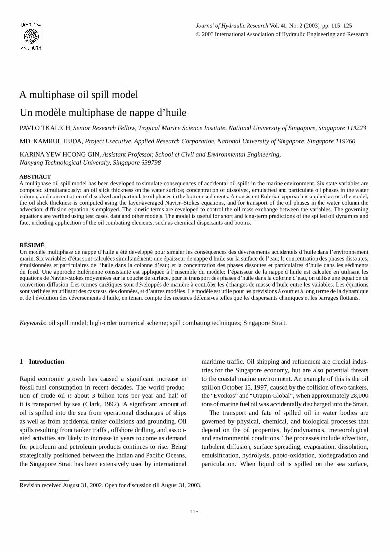
Equation (1a) for the oil slick dynamics was derived fromthe Navier–Stokes equations, averaged over the slick thick-ness (Warluzel and Benque, 1981). The second term of theequation governs the slick horizontal drift, associated with thecombined action of wind and surface current, and the thirdterm is for the slick spreading due to gravity–viscosity forces.The set of advection–diffusion Eq. (1b) describes transport ofthe oil phases in the water column. Terms in the right-handside of Eqs. (1) identify the oil mass transfer between thephases (emulsified, dissolved and particulate) and the media(slick, water column and bed sediments) according to the pre-scribed kinetics (Figure 1). It is assumed that oil from theslick may enter into the water column to form emulsified anddissolved oil phases, and to adsorb to suspended and bottomsediments. The total amount of oil is divided according to theproperties of three fractions: the heavy fraction that is able toproduce an oil-in-water emulsion(ke), the light fraction thatis likely to evaporate or dissolve(kd), and the residual frac-tion (kr). The respective oil kinetics is governed by the followingequations:

Rh ≡ ∂h

∂t= −Ksvh

}in the slick (2a)

Figure 1 Oil mass transfer chart.

Re ≡ ∂Ce

∂t= −KeSw(aeCe − Cp)

Rd ≡ ∂Cd

∂t= −KdSw(adCd − Cp)

Rp ≡ ∂Cp

∂t= Ke(aeCe − Cp)

+Kd(adCd − Cp)

in the water column (2b)

dCdb

dt= −K ′

dρs(a′dCdb − Cpb)

dCpb

dt= K ′

d(a′dCdb − Cpb)

in the bed sediments (2c)

Here,{K, K ′} are the oil mass exchange rate coefficients,{a, a′}are the partition coefficients,Ksv is the oil evaporation rate fromthe slick,Cpb andCdb are the concentrations of particulate anddissolved oil in the bed sediments,ρs is the density of the bedsediments,Sw is the characteristic concentration of the suspendedsediments. If values ofCe, Cd, andCdb are given in [g-of-oil/m3],Cp andCpb are in [g-of-oil/kg-of-sediments], thenae, ad anda′

d

must be expressed in [m3/kg-of-sediments]. The water column isbounded by the oil slick on the surface, and by the bed sedimentson the bottom (Figure 1). The whole system “oil slick – water col-umn – bed sediments” consists of three layers and two interfaces,where the oil mass transfer kinetics have to be specified.

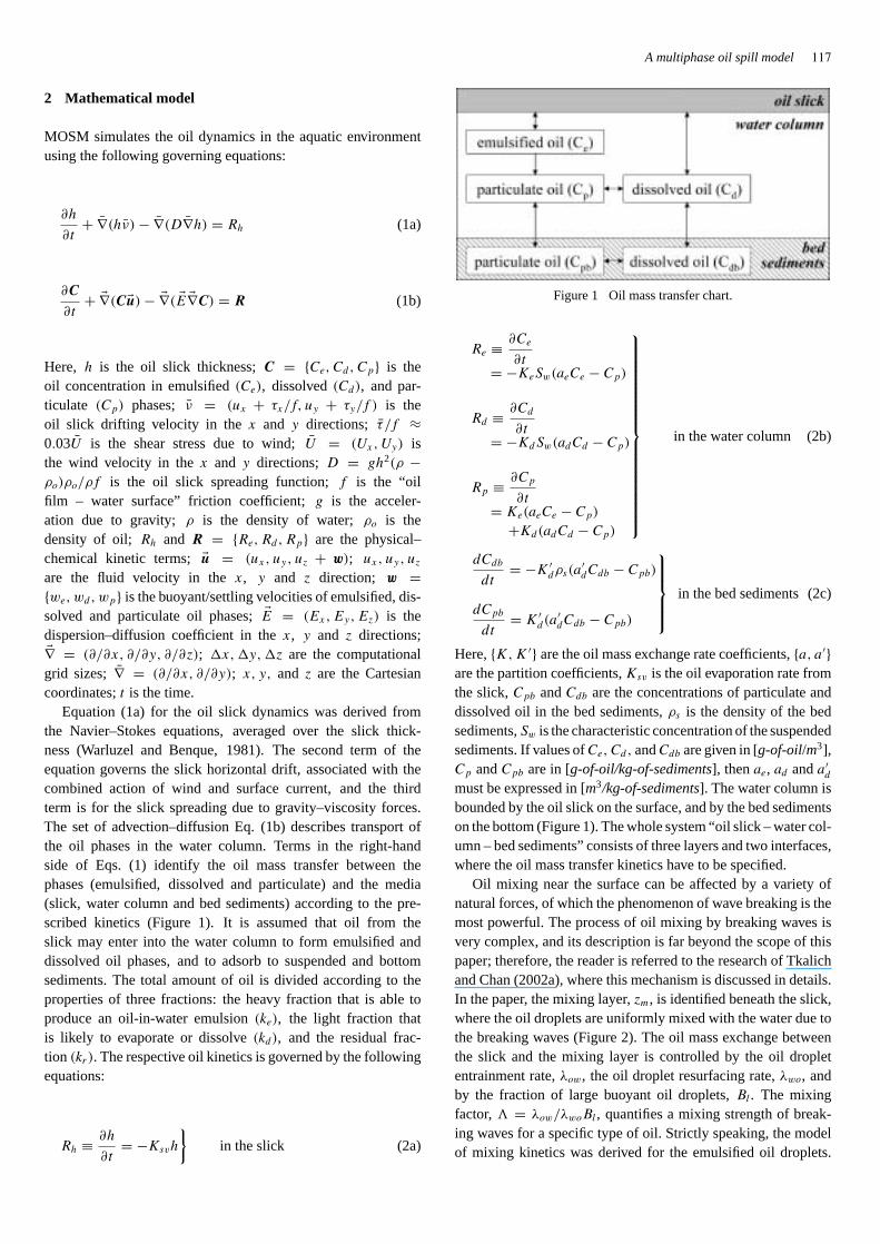
Oil mixing near the surface can be affected by a variety ofnatural forces, of which the phenomenon of wave breaking is themost powerful. The process of oil mixing by breaking waves isvery complex, and its description is far beyond the scope of thispaper; therefore, the reader is referred to the research of Tkalichand Chan (2002a), where this mechanism is discussed in details.In the paper, the mixing layer,zm, is identified beneath the slick,where the oil droplets are uniformly mixed with the water due tothe breaking waves (Figure 2). The oil mass exchange betweenthe slick and the mixing layer is controlled by the oil dropletentrainment rate,λow, the oil droplet resurfacing rate,λwo, andby the fraction of large buoyant oil droplets,Bl . The mixingfactor,� = λow/λwoBl , quantifies a mixing strength of break-ing waves for a specific type of oil. Strictly speaking, the modelof mixing kinetics was derived for the emulsified oil droplets.

118 Pavlo Tkalich et al.

Figure 2 Vertical structure of the water column. Sketch of the mixing layer and the computational grid.

Since, submerged droplets increase the contact surface area ofoil and water, leading to higher rate of oil dissolution, onecan use the mixing factor to quantify the rate of oil dissolutionas well.

Oil exchange at the interfaces “oil slick – water column” and“water column – bed sediments” can be quantified using thefollowing kinetics

dh

dt= −Kes(aesρo − Ce)

zm

ρo

− Kds(adsC∗ − Cd)zm

ρo

dCe

dt= Kes(aesρo − Ce),

dCd

dt= Kds(adsC∗ − Cd)

at the “oil slick – water column” interface (3a)

dCd

dt= Kdb(adbCdb − Cd),

dCp

dt= Kpb(apbCpb − Cp)

dCdb

dt= −Kdb(adbCdb − Cd)

zb

b

dCpb

dt= −Kpb(apbCpb − Cp)

zbSw

ρs(1 − φ)b

at the “water column – bed sendiments” interface (3b)

Here, {K} are the oil mass exchange rates,{a} are the parti-tion coefficients,C∗ is the saturation concentration of the oil’slight fraction,zb is the thickness of the near-bottom layer of thewater column (one can assumezb = �z), b is the thickness ofactive layer of the bed sediments,φ is the porosity of the bedsediments. To match the oil mixing kinetics model (Tkalich andChan, 2002a), one has to assignKes = (λow + λwo)/(1 + �),aes = �h/zm, Kds ∼ (λow + λwo)/(1 + �) andads ∼ �h/zm.Application of the two-layer diffusion model (Clark, 1996) atthe “water column – bed sediments” interface gives the approx-imationKdb = EwEb/(bEw + zbEb)zb, whereEb andEw arethe diffusion coefficients in the interstitial and overlying water,respectively. Alternatively, the coefficients{K, K ′} and {a, a′}can be obtained by fitting the model to empirical data.

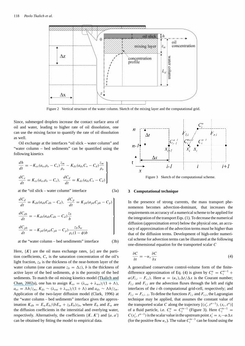
Figure 3 Sketch of the computational scheme.

3 Computational technique

In the presence of strong currents, the mass transport phe-nomenon becomes advection-dominant, that increases therequirements on accuracy of a numerical scheme to be applied forthe integration of the transport Eqs. (1). To decrease the numericaldiffusion (approximation error) below the physical one, an accu-racy of approximation of the advection terms must be higher thanthat of the diffusion terms. Development of high-order numeri-cal scheme for advection terms can be illustrated at the followingone-dimensional equation for the transported scalarC

∂C

∂t= −ux

∂C

∂x(4)

A generalised conservative control-volume form of the finite-difference approximation of Eq. (4) is given byCn

i = Cn−1i +

α(Fl,i − Fr,i). Hereα = (ux)i�t/�x is the Courant number;Fl,i andFr,i are the advection fluxes through the left and rightinterfaces of thei-th computational grid-cell, respectively; andFl,i = Fr,i−1. To define the functionsFl,i andFr,i , the Lagrangiantechnique may be applied, that assumes the constant value ofthe transported scalarC along the trajectory[(x ′

i , tn−1), (xi, t

n)]of a fluid particle, i.e.Cn

i = C ′n−1i (Figure 3). HereC ′n−1

i =C(x ′

i , tn−1) is the scalar value in the upstream pointx ′

i = xi−α�x

(for the positive flowux). The valueC ′n−1i can be found using the

A multiphase oil spill model 119

piece-wise interpolation polynomialPi(α), resulting in the finite-difference schemeCn

i = Pi(α). Them-th degree polynomial maytake the following form

Pi(αi) =m∑

j=0

Mj,iαj

where the coefficientsMj,i are found by requiring that the poly-nomial passes through all grid points of the computational stencil.Depending on valuem, one can obtain first-order approximationfor m = 1, second-order form = 2, and third-order form = 3,the latter is also known as the QUICKEST scheme (Leonard,1984); i.e.

Fl,i = Cn−1i−1 , m = 1 (5a)

Fl,i = 0.5(Cn−1

i + Cn−1i−1

) − 0.5α(Cn−1

i − Cn−1i−1

)

−0.5(1 − α)(Cn−1

i − 2Cn−1i−1 + Cn−1

i−2

), m = 2 (5b)

Fl,i = 0.5(Cn−1

i + Cn−1i−1

) − 0.5α(Cn−1

i − Cn−1i−1

)

−(1 − α2)(Cn−1

i − 2Cn−1i−1 + Cn−1

i−2

)/6, m = 3 (5c)

As an example of the spreading/diffusion terms approximationin Eqs. (1), one can consider the simplified one-dimensionalequation

∂C

∂t= ∂

∂x

(E

∂C

∂x

)(6)

To solve Eq. (6) in the conservative control-volume manner,Cn

i = Cn−1i +µ(Fdr,i −Fdl,i ), one can apply the centered-space-

forward-time (CSFT) second-order numerical scheme, yieldingFdl,i = 0.5(En−1

i +En−1i−1 )(Cn−1

i −Cn−1i−1 ). Hereµ = �t/(�x)2;

Fdl,i andFdr,i are the diffusion fluxes through the left and rightinterfaces of thei-th computational grid-cell, respectively; andFdl,i = Fdr,i−1.

The same approximation technique, Eq. (5c), of advectionterms was applied by Tkalich and Chan (2002b) for deriva-tion of the two-dimensional Third Order Polynomial (TOP)method, having an advective flux through the right interface of

(a)1 (b)

0.5

0

1

0.5

0

0

200,000

x (m)

200.000

0

y (m)

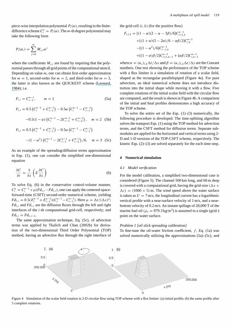
Figure 4 Simulation of the scalar field rotation in 2-D circular flow using TOP scheme with a flux limiter: (a) initial profile; (b) the same profile after5 complete rotations.

the grid-cell(i, k) (for the positive flow)

Fr,i,k = [(1 − α)(2 − α − 3β)/6]Cn−1i+1,k

+[(1 + α)(5 − 2α)/6 − αβ/2]Cn−1i,k

−[(1 − α2)/6]Cn−1i−1,k

+[(1 − α)β/2]Cn−1i+1,k−1 + [αβ/2]Cn−1

i,k−1

whereα = (ux)i,k�t/�x andβ = (uy)i,k�t/�y are the Courantnumbers. One test showing the performance of the TOP schemewith a flux limiter is a simulation of rotation of a scalar field,shaped as the rectangular parallelepiped (Figure 4a). For pureadvection, an ideal numerical scheme does not introduce dis-tortion into the initial shape while moving it with a flow. Fivecomplete rotations of the initial scalar field with the circular floware computed, and the result is shown in Figure 4b. A comparisonof the initial and final profiles demonstrates a high accuracy ofthe TOP scheme.

To solve the entire set of the Eqs. (1)–(3) numerically, thefollowing procedure is developed. The time-splitting algorithmsolves the transport Eqs. (1) using the TOP method for advectionterms, and the CSFT method for diffusion terms. Separate sub-modules are applied for the horizontal and vertical terms using 2-D and 1-D versions of the TOP-CSFT scheme, respectively. Thekinetic Eqs. (2)–(3) are solved separately for the each time-step.

4 Numerical simulation

4.1 Model verification

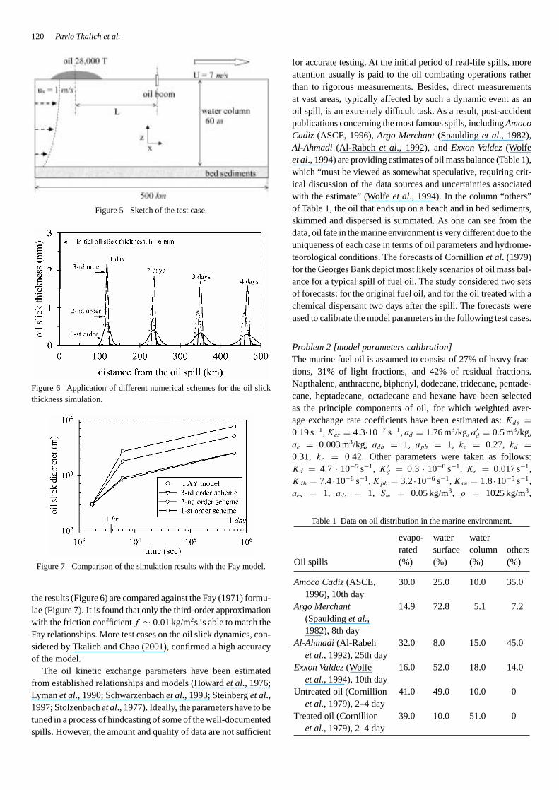
For the model calibration, a simplified two-dimensional case isconsidered (Figure 5). The channel 500 km long, and 60 m deepis covered with a computational grid, having the grid-size(�x ×�z) = (1000× 5) m. The wind speed above the water surfaceis taken asU = 7 m/s, the longitudinal current has a logarithmicvertical profile with a near-surface velocity of 1 m/s, and a near-bottom velocity of 0.2 m/s. An instant spillage of 28,000 T of themarine fuel oil(ρo = 979.3 kg/m3) is assumed in a single (grid-)point on the water surface.

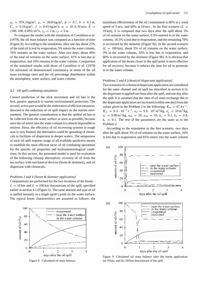
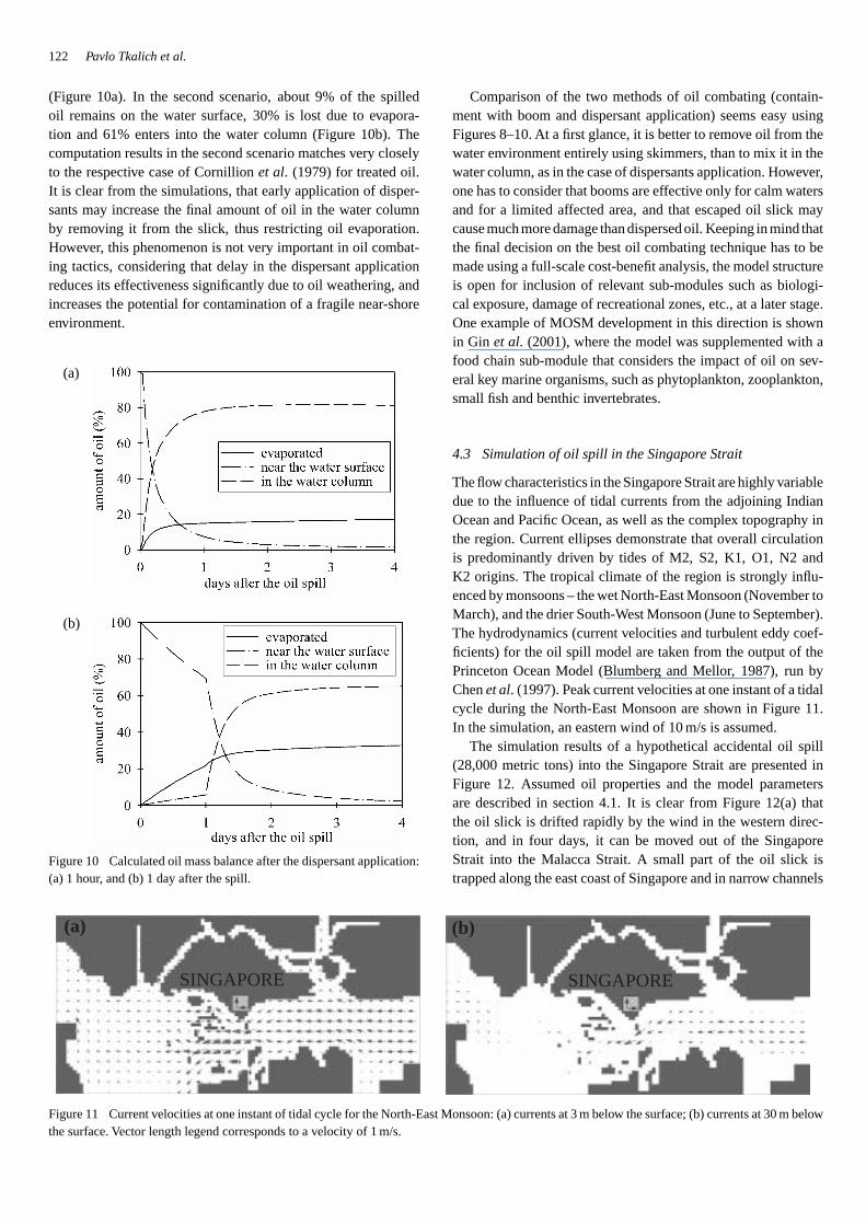
Problem 1 [oil slick spreading calibration]To fine-tune the oil-water friction coefficient,f , Eq. (1a) wassolved numerically utilizing the approximations (5a)–(5c), and

120 Pavlo Tkalich et al.

Figure 5 Sketch of the test case.

Figure 6 Application of different numerical schemes for the oil slickthickness simulation.

Figure 7 Comparison of the simulation results with the Fay model.

the results (Figure 6) are compared against the Fay (1971) formu-lae (Figure 7). It is found that only the third-order approximationwith the friction coefficientf ∼ 0.01 kg/m2s is able to match theFay relationships. More test cases on the oil slick dynamics, con-sidered by Tkalich and Chao (2001), confirmed a high accuracyof the model.

The oil kinetic exchange parameters have been estimatedfrom established relationships and models (Howardet al., 1976;Lymanet al., 1990; Schwarzenbachet al., 1993; Steinberget al.,1997; Stolzenbachet al., 1977). Ideally, the parameters have to betuned in a process of hindcasting of some of the well-documentedspills. However, the amount and quality of data are not sufficient

for accurate testing. At the initial period of real-life spills, moreattention usually is paid to the oil combating operations ratherthan to rigorous measurements. Besides, direct measurementsat vast areas, typically affected by such a dynamic event as anoil spill, is an extremely difficult task. As a result, post-accidentpublications concerning the most famous spills, includingAmocoCadiz (ASCE, 1996),Argo Merchant (Spauldinget al., 1982),Al-Ahmadi (Al-Rabehet al., 1992), andExxon Valdez (Wolfeet al., 1994) are providing estimates of oil mass balance (Table 1),which “must be viewed as somewhat speculative, requiring crit-ical discussion of the data sources and uncertainties associatedwith the estimate” (Wolfeet al., 1994). In the column “others”of Table 1, the oil that ends up on a beach and in bed sediments,skimmed and dispersed is summated. As one can see from thedata, oil fate in the marine environment is very different due to theuniqueness of each case in terms of oil parameters and hydrome-teorological conditions. The forecasts of Cornillionet al. (1979)for the Georges Bank depict most likely scenarios of oil mass bal-ance for a typical spill of fuel oil. The study considered two setsof forecasts: for the original fuel oil, and for the oil treated with achemical dispersant two days after the spill. The forecasts wereused to calibrate the model parameters in the following test cases.

Problem 2 [model parameters calibration]The marine fuel oil is assumed to consist of 27% of heavy frac-tions, 31% of light fractions, and 42% of residual fractions.Napthalene, anthracene, biphenyl, dodecane, tridecane, pentade-cane, heptadecane, octadecane and hexane have been selectedas the principle components of oil, for which weighted aver-age exchange rate coefficients have been estimated as:Kds =0.19 s−1, Kes = 4.3·10−7 s−1, ad = 1.76 m3/kg,a′

d = 0.5 m3/kg,ae = 0.003 m3/kg, adb = 1, apb = 1, ke = 0.27, kd =0.31, kr = 0.42. Other parameters were taken as follows:Kd = 4.7 · 10−5 s−1, K ′

d = 0.3 · 10−8 s−1, Ke = 0.017 s−1,Kdb = 7.4·10−8 s−1, Kpb = 3.2·10−6 s−1, Ksv = 1.8·10−5 s−1,aes = 1, ads = 1, Sw = 0.05 kg/m3, ρ = 1025 kg/m3,

Table 1 Data on oil distribution in the marine environment.

evapo- water waterrated surface column others

Oil spills (%) (%) (%) (%)

Amoco Cadiz (ASCE,1996), 10th day

30.0 25.0 10.0 35.0

Argo Merchant(Spauldinget al.,1982), 8th day

14.9 72.8 5.1 7.2

Al-Ahmadi (Al-Rabehet al., 1992), 25th day

32.0 8.0 15.0 45.0

Exxon Valdez (Wolfeet al., 1994), 10th day

16.0 52.0 18.0 14.0

Untreated oil (Cornillionet al., 1979), 2–4 day

41.0 49.0 10.0 0

Treated oil (Cornillionet al., 1979), 2–4 day

39.0 10.0 51.0 0

A multiphase oil spill model 121

ρo = 979.3 kg/m3, ρs = 2650 kg/m3, φ = 0.7, b = 0.1 m,C∗ = 0.54 g/m3, f = 0.01 kg/m2s, w = {0, 0, 0} m/s, �E =(100, 100, 0.001) m2/s,zm = 1 m,zb = 5 m.

To compare the model with the simulation of Cornillionet al.(1979), the oil mass balance was computed as a function of time(Figure 8). According to the simulation, after one day about 25%of the total oil is lost by evaporation, 5% enters the water column,70% remains on the water surface. After two days, about 49%of the total oil remains on the water surface, 41% is lost due toevaporation, and 10% remains in the water column. Comparisonof the simulated results with those of Cornillionet al. (1979)for untreated oil demonstrated consistency in terms of the oilmass exchange rates and the oil percentage distribution withinthe atmosphere, water surface, and water column.

4.2 Oil spill combating simulation

Correct prediction of the slick movement and oil fate is thefirst, passive approach to marine environmental protection. Thesecond, active part would be the elaboration of efficient measures,directed to the reduction of oil spill impact on the marine envi-ronment. The general consideration is that the spilled oil has tobe collected from the water surface as soon as possible, becauseonce the oil enters into the water column it is almost impossible toretrieve. Since, the efficiency of oil recovering systems in roughseas is very limited, the alternative could be spreading of chemi-cals to facilitate oil dispersion in deeper waters. The uniquenessof each oil spill requires usage of all available predictive meansto establish the most efficient tactic of oil combating operationsfor the specific oil properties and hydrometeorological condi-tions. In this section, the presented model is used for evaluationof the following cleanup alternatives: recovery of oil from thesea surface with mechanical devices (boom & skimmer), and oildispersion with chemicals.

Problems 3 and 4 [boom & skimmer application]Computations are performed for the two locations of the boom –L = 10 km andL = 100 km downstream of the spill, specifiedearlier in section 4.1 (Figure 5). The same amount and type of oilis spilled instantly in a single (grid-) point on the water surface.The typical boom characteristics are assumed as follows: the

Figure 8 Calculated oil mass balance.

maximum effectiveness of the oil containment is 80% at a windspeed of 5 m/s, and 60% at 10 m/s . In the first scenario (L =10 km), it is computed that two days after the spill about 3%of oil remains on the water surface, 0.5% entered in to the watercolumn, 18.5% is lost due to evaporation, and the remaining 78%is recovered by the skimmer (Figure 9a). In the second scenario(L = 100 km), about 5% of oil remains on the water surface,3% in the water column, 32% is lost due to evaporation, and60% is recovered by the skimmer (Figure 9b). It is obvious thatapplication of the boom closer to the spill point is more effectivefor oil recovery, because it reduces the time for oil to penetratein to the water column.

Problems 5 and 6 [chemical dispersant application]Two scenarios of a chemical dispersant application are consideredfor the same channel and oil spill (as described in section 4.1):the dispersant is applied one hour after the spill, and one day afterthe spill. It is assumed that the rates of oil mass exchange due tothe dispersant application are increased (within one day) from thevalues given in the Problem 2 to the following:Kds = 47.4 s−1,Kes = 9.3 · 10−7 s−1, ad = 9.8 · 102 m3/kg, a′

d = 10 m3/kg,ae = 0.89 m3/kg, adb = 10, apb = 10, ke = 0.1, kd = 0.8,kr = 0.1. The rest of the parameters are the same as in theProblem 2.

According to the simulation in the first scenario, two daysafter the spill about 3% of oil remains on the water surface, 16%is lost due to evaporation and 81% enters into the water column

(a)

(b)

Figure 9 Calculated oil mass balance after the boom application:(a) 10 km, and (b) 100 km downstream of the spill.

122 Pavlo Tkalich et al.

(Figure 10a). In the second scenario, about 9% of the spilledoil remains on the water surface, 30% is lost due to evapora-tion and 61% enters into the water column (Figure 10b). Thecomputation results in the second scenario matches very closelyto the respective case of Cornillionet al. (1979) for treated oil.It is clear from the simulations, that early application of disper-sants may increase the final amount of oil in the water columnby removing it from the slick, thus restricting oil evaporation.However, this phenomenon is not very important in oil combat-ing tactics, considering that delay in the dispersant applicationreduces its effectiveness significantly due to oil weathering, andincreases the potential for contamination of a fragile near-shoreenvironment.

(a)

(b)

Figure 10 Calculated oil mass balance after the dispersant application:(a) 1 hour, and (b) 1 day after the spill.

SINGAPORE

(b)

SINGAPORE

(a)

Figure 11 Current velocities at one instant of tidal cycle for the North-East Monsoon: (a) currents at 3 m below the surface; (b) currents at 30 m belowthe surface. Vector length legend corresponds to a velocity of 1 m/s.

Comparison of the two methods of oil combating (contain-ment with boom and dispersant application) seems easy usingFigures 8–10. At a first glance, it is better to remove oil from thewater environment entirely using skimmers, than to mix it in thewater column, as in the case of dispersants application. However,one has to consider that booms are effective only for calm watersand for a limited affected area, and that escaped oil slick maycause much more damage than dispersed oil. Keeping in mind thatthe final decision on the best oil combating technique has to bemade using a full-scale cost-benefit analysis, the model structureis open for inclusion of relevant sub-modules such as biologi-cal exposure, damage of recreational zones, etc., at a later stage.One example of MOSM development in this direction is shownin Gin et al. (2001), where the model was supplemented with afood chain sub-module that considers the impact of oil on sev-eral key marine organisms, such as phytoplankton, zooplankton,small fish and benthic invertebrates.

4.3 Simulation of oil spill in the Singapore Strait

The flow characteristics in the Singapore Strait are highly variabledue to the influence of tidal currents from the adjoining IndianOcean and Pacific Ocean, as well as the complex topography inthe region. Current ellipses demonstrate that overall circulationis predominantly driven by tides of M2, S2, K1, O1, N2 andK2 origins. The tropical climate of the region is strongly influ-enced by monsoons – the wet North-East Monsoon (November toMarch), and the drier South-West Monsoon (June to September).The hydrodynamics (current velocities and turbulent eddy coef-ficients) for the oil spill model are taken from the output of thePrinceton Ocean Model (Blumberg and Mellor, 1987), run byChenet al. (1997). Peak current velocities at one instant of a tidalcycle during the North-East Monsoon are shown in Figure 11.In the simulation, an eastern wind of 10 m/s is assumed.

The simulation results of a hypothetical accidental oil spill(28,000 metric tons) into the Singapore Strait are presented inFigure 12. Assumed oil properties and the model parametersare described in section 4.1. It is clear from Figure 12(a) thatthe oil slick is drifted rapidly by the wind in the western direc-tion, and in four days, it can be moved out of the SingaporeStrait into the Malacca Strait. A small part of the oil slick istrapped along the east coast of Singapore and in narrow channels

A multiphase oil spill model 123

(b) droplet concentration at depth 3 m [kg/cub.m]

(a) slick thickness [m] (c) droplet concentration at depth 20 m [kg/cub.m]

0.5

day

1.5

day

2.5

day

3.5

day

(c.3)

(c.4)(b.4)

(b.3)(a.3)

(a.4)

(c.2)(b.2)(a.2)

(b.1) (c.1)(a.1)

Figure 12 Computed oil dynamics in the Singapore Strait at different time after the spill: (a) oil slick thickness; (b) concentration of the emulsifiedoil at depths 3 m, and (c) 20 m below the water surface. Rows 1 to 4 correspond to 0.5, 1.5, 2.5 and 3.5 days after the spill, respectively. Initial locationof the spill is shown by a star in Figure (a.1).

between the southern islands. Due to less exposure to the windaction, oil droplets are likely to persist in the water column for amuch longer time before the tidal currents are able to disperse it(Figures 12b,c). It is predicted that a significant amount of sub-surface oil can be trapped in shallow waters of the Singaporecoast, as well as stranded at the shoreline.

5 Conclusions

A three-dimensional multiphase oil spill model has been devel-oped to simulate the consequences of accidental oil releases inthe ocean environment. It was shown, that to match empiricaldata, a high-order numerical approximation of governing equa-tions is required. Test simulations of oil slick dynamics, as wellas transport and kinetics of the oil phases in the water column,show good consistency with empirical data and other models.The calculations clearly demonstrated that contamination of thewater column with oil may remain high for days after the slickdisappears from the site. Therefore, to simulate correctly thelong-term consequences of surface spills, one has to take intoaccount subsurface fractions of oil as well.

Due to its versatility, the model can be applied for evaluationof oil spill countermeasures in complicated meteorological andhydrodynamic conditions. The two most popular countermea-sures, such as floating booms and chemical dispersants, wereanalysed numerically. Though the model is able to predict theconcentration of oil in different phases very accurately, the finaldecision on the best oil combating tactic should be made onlyafter application of a full-scale cost-benefit analysis, includingbiological and economic sub-modules.

Notations

ad, a′d = “suspended sediments – water column” and “bed

sediments – pore water” dissolved oil distributioncoefficients

adb, apb = “bed sediments – water column” dissolved andparticulate oil distribution coefficients

ae = “suspended sediments – water column” emulsifiedoil distribution coefficient

aes, ads = “slick – water column” emulsified and dissolved oildistribution coefficients

b = thickness of active bed sediments

124 Pavlo Tkalich et al.

Bl = fraction of large (buoyant) dropletsCn

i = value of the scalarC at the grid pointxi at the timetn

C = {Ce, Cd, Cp} = oil concentration in water column inemulsified, dissolved and particulatephases

C∗ = saturation concentration of the oil’slight fraction

Cdb, Cpb = oil concentration in bed sediments indissolved and particulate phases

D = oil slick spreading-diffusion func-tion

�E = (Ex, Ey, Ez) = dispersion–diffusion coefficients inwater column

Eb, Ew = dispersion–diffusion coefficients inthe near-bottom water layer and ininterstitial water of bed sediments

Fl, Fr = left- and right-face advection fluxesFdl , Fdr = left- and right-face diffusion fluxes

f = oil film – water surface friction coef-ficient

g = acceleration due to gravityh = oil slick thickness

i, k = grid-node indexesKd, K

′d = adsorption rate of the dissolved oil

in the water column and in the bedsediments

Ke = adsorption rate of the emulsified oilin the water column

Kds, Kes, Ksv = dissolution, emulsification and evap-oration rates of oil from slick

Kdb, Kpb = “water column – bed sediments” dis-solved and particulate oil exchangerates

ke, kd, kr = heavy, light and residual oil frac-tions

L = distance between oil spill locationand boom

Mj = polynomial coefficientsm = degree of interpolation polynomialn = time indexP = interpolation polynomial

R = {Re, Rd, Rp}, Rh = oil kinetic termsSw = suspended sediment concentration

t = time variableU = (Ux, Uy) = wind velocity

ux, uy, uz = current velocityν = (νx, νy) = oil slick movement velocity

w = {we, wd, wp} = buoyant/settling velocities of oilphases

x, y, z = Cartesian coordinatesxi = grid-points along axisx

zb, zm = thickness of near-bottom and near-surface water layers

�t = computational time step�x, �z = computational grid size

α, β = Courant numbersφ = porosity of bed sediments� = mixing factor

λow, λwo = oil droplet entrainment and resur-facing rates

µ = diffusion numberρ, ρo, ρs = density of water, oil and bottom

sedimentsτ = (τx, τy) = shear stress due to wind

∇ = (∂/∂x, ∂/∂y) = 2-D space gradient�∇ = (∂/∂x, ∂/∂y, ∂/∂z) = 3-D space gradient

References

1. Al-Rabeh, A.H., Cekirge, H.M. and Gunay N. (1992).“Modeling the Fate and Transport of Al-Ahmadi Oil Spill”,Water, Air, and Soil Pollution, 65, 257–279.

2. ASCE Task Committee on Modeling of Oil Spills of theWater Resources Engineering Division (1996). “State-of-the-art Review of Modeling Transport and Fate of OilSpills”, J. Hydr. Engrg., 122, 594–609.

3. Blumberg, A.F. and Mellor, G.L. (1987). A descriptionof a three-dimensional coastal ocean circulation model, in“Three-Dimensional Coastal Ocean Model” edited by N.S.Heaps, p. 208, American Geophysical Union.

4. Chen, M., Khoo, B.C. and Chan, E.S. (1997). “ThreeDimensional Circulation Model of Singapore CoastalWaters”, Proc. of the Conf. Oceanology International’97Pacific Rim, 1, 281–291.

5. Clark, M.M. (1996). Transport modeling for environmen-tal engineers and scientists. J.Wiley & Sons, NY, USA,p. 559.

6. Clark, R.B. (1992). Marine Pollution. 3rd ed., GookcraftLtd., Great Britain, UK, pp. 50–60.

7. Cornillon, P.C., Spaulding, M.L. and Hansen, K. (1979).“Oil Spill Treatment Strategy Modeling for Georges Bank”,Proc. of the 1979 Oil Spill Conference, 685–692.

8. Delvigne, G.A.L. and Sweeney, C.E. (1988). “NaturalDispersion of Oil”,Oil & Chemical Pollution, 4, 281–310.

9. Fay, J.A. (1971). “Physical Processes in the Spread of Oil ona Water Surface”,Proc. of the Joint Conf. On the Preventionand Control of Oil Spills, 463-467.

10. Gin, K., Huda, K., Lim, W.K. and Tkalich, P. (2001). “Anoil spill – Food Chain Interaction Model for CoastalWaters”,Marine Pollution Bulletin, 42(7), 590–597.

11. Howard, P.H., Sage, G.W., Michalenko, E.M., Basu,D.K., Hill, A. andAronson, D. (1976). Handbook of Envi-ronmental Fate and Exposure Data For Organic Chemistry.Lewis Publishers, Inc., Michigan, USA, pp. 260–461.

12. Huang, J.C. (1983). “A Review of the State-of-the-art of OilSpill Fate/Behaviour Models”,Proc. of the 1983 Oil SpillConference. Washington DC, API, 313–322.

13. Lehr, W.J., Cekirge, H.M., Fraga, R.J. and Belen, M.S.(1984). “Empirical Studies of the Spreading of Oil Spills”,Oil and Petrochemical Poll., 2, 7–11.

A multiphase oil spill model 125

14. Leonard, B.P. (1984). “Third-order Upwinding as a Ratio-nal Basis for Computational Fluid Dynamics”, inProc. ofthe International Computational Techniques and Applica-tions Conference (CTAC-83), The University of Sydney,Australia, 1983, Elsevier Science Pub. Co., pp. 106–120.

15. Lyman, W.J., Reehl, W.F. and Rosenblatt, D.H. (1990).Handbook of Chemical Property Estimation Methods –Environmental Behavior of Organic Compound. AmericanChemical Society, Washington DC, USA, pp. 4-12.

16. Mackay, D., Paterson, S. and Trudel, K. (1980).A mathematical model of oil spill behavior. Environmen-tal Protection Service, Fisheries and Environment CanadaReport EE-7.

17. Reed, M., Johansen, O., Brandvik, P.J., Daling, P.,Lewis, A., Fiocco, R., Mackay, D. and Prentki, R.(1999). “Oil Spill Modelling Toward the Close of the 20thCentury: Overview of the State of the Art”,Spill Scienceand Technology Bulletin, 5, 3–16.

18. Schwarzenbach, R.P., Gschwend, P.M. and Imboden,D.M. (1993). Environmental Organic Chemistry. A Wiley-Interscience Publication, John Wiley & Son, Inc., NY, USA,pp. 238–242.

19. Spaulding, M.L. (1988). “A State-of-the-art Review ofOil Spill Trajectory and Fate Modeling”,Oil and ChemicalPollution, (4), 39–55.

20. Spaulding, M.L., Jayko, K. E. and Anderson, E.L.(1982). “Hindcast of theArgo Merchant Spill Using the URIOil Spill Fates Model”,Ocean Engineering, 9(5), 455–482.

21. Steinberg, L.J., Reckhow, K.H. and Wolpert, R.L.(1997). “Characterization of Parameters in MechanisticModels: A Case Study of a PCB Fate and Transport Model”,Ecological Modelling, 97, 35–46.

22. Stolzenbach, K.D., Madsen, O.S., Adams, E.E.,Pollack, A.M. and Cooper, C.K. (1977). A Reviewand Evaluation of Basic Techniques for Predicting theBehavior of Surface Oil Slicks. Report No. 222,Ralph M. Parsons Laboratory For Water Resourcesand Hydrodynamics, Department of Civil Engineering,MIT, USA.

23. Tkalich, P. (2002). “Oil Spill Modelling with a CFDApproach”, Proc. of Sixth International Marine Envi-ronmental Modelling Seminar, 2–4 September 2002,Trondheim, Norway, 255–274.

24. Tkalich, P. and Chan, E.S. (2002a). “Vertical Mixing of OilDroplets by Breaking Waves”,Marine Pollution Bulletin,44(11), 1219–1229.

25. Tkalich, P. and Chan, E.S. (2002b). “The Third-orderPolynomial Method for Two-dimensional Convection andDiffusion”, Int. J. for Numerical Methods in Fluids(submitted).

26. Tkalich, P. and Chao, X.B. (2001). “Accurate Simula-tion of Oil Slicks”, Proc. of the International Oil SpillConference, 26–29 March 2001, Tampa, Florida, USA,1133–1137.

27. Warluzel, A. and Benque, J.P. (1981). “Un ModèleMathématique De Transport Et D’Etalement D’Une NappeD’Hydrocarbures”,Proc. of Conf. Mechanics of Oil Slicks,Paris, 199–211.

28. Wolfe, D.A., Hameedi, M.J., Galt, J.A., Watabayashi,G., Short, J., O’Claire, C., Rice, S., Michel, J.,Payne, J.R., Braddock, J., Hanna, S. and Sale, D.(1994). “The Fate of the Oil Spilled from the ExxonValdez”, Environmental Science and Technology, 28(13),561–568.