www.elsevier.com/locate/geomorph

Geomorphology 74

A landslide susceptibility model using the Analytical Hierarchy

Process method and multivariate statistics in perialpine Slovenia

Marko Komac *

Geological Survey of Slovenia, Dimiceva 14, SI-1000 Ljubljana, Slovenia

Received 15 March 2004; received in revised form 1 June 2005; accepted 17 July 2005

Available online 24 August 2005

Abstract

Landslides cause damage to property and unfortunately pose a threat even to human lives. Good landslide susceptibility,

hazard, and risk models could help mitigate or even avoid the unwanted consequences resulted from such hillslope mass

movements. For the purpose of landslide susceptibility assessment the study area in the central Slovenia was divided to 78365

slope units, for which 24 statistical variables were calculated. For the land-use and vegetation data, multi-spectral high-

resolution images were merged using Principal Component Analysis method and classified with an unsupervised classification.

Using multivariate statistical analysis (factor analysis), the interactions between factors and landslide distribution were tested,

and the importance of individual factors for landslide occurrence was defined. The results show that the slope, the lithology, the

terrain roughness, and the cover type play important roles in landslide susceptibility. The importance of other spatial factors

varies depending on the landslide type. Based on the statistical results several landslide susceptibility models were developed

using the Analytical Hierarchy Process method. These models gave very different results, with a prediction error ranging from

4.3% to 73%. As a final result of the research, the weights of important spatial factors from the best models were derived with

the AHP method. Using probability measures, potentially hazardous areas were located in relation to population and road

distribution, and hazard classes were assessed.

D 2005 Elsevier B.V. All rights reserved.

Keywords: Landslide susceptibility; Multivariate analysis; Analytical Hierarchy Process; Slovenia

1. Introduction

Recent natural disasters in Europe, like the floods

in 2002 (BBC, 2002) and numerous hillslope mass

movements that have occurred in the course in recent

0169-555X/$ - see front matter D 2005 Elsevier B.V. All rights reserved.

doi:10.1016/j.geomorph.2005.07.005

* Tel.: +386 2809700; fax: +386 1 2809753.

E-mail address: marko.komac@geo-zs.si.

years, have augmented the need for a better under-

standing of these natural phenomena. Geohazards,

such as landslides, floods or earthquakes, are a source

of concern around the world and Slovenia is no

exception. Such events are generally the result of

natural forces, seldom the consequence of human

action. Whatever the cause, their prevention or miti-

gation is an important step towards the preservation of

(2006) 17–28

M. Komac / Geomorphology 74 (2006) 17–2818

the environmental quality. Hence the need for a better

understanding of these phenomena, especially when

their triggering factors can be to some measure con-

trolled, as in the case of landslides.

Landslides are the result of two interacting sets of

forces; the precondition factors, generally naturally

induced, which govern the stability conditions of

slopes, and the preparatory and the triggering factors,

induced either by natural factors or by human inter-

vention. These triggers are usually intensive, geologi-

cally speaking short-term processes that irreversibly

change the slope and cause the landslide (Glade and

Crozier, 2005).

The scope of the paper is to examine the long-term

factors, and to define their relations to landslide occur-

rence in the studied area. The primary goal was to

study spatial factors that conjointly influence the

occurrence of landslides, and to statistically establish

the multivariate relations of the independent factors

with the spatial distribution of landslides. The second

goal was to create a landslide susceptibility model,

based on the statistical relationships that would help to

predict the landslide prone areas with a high reliabil-

ity, not only in the studied area. Additionally, the

results of such a study would define hazardous

areas, where landslides might occur over short-term

timescales. As a final goal of the research, superim-

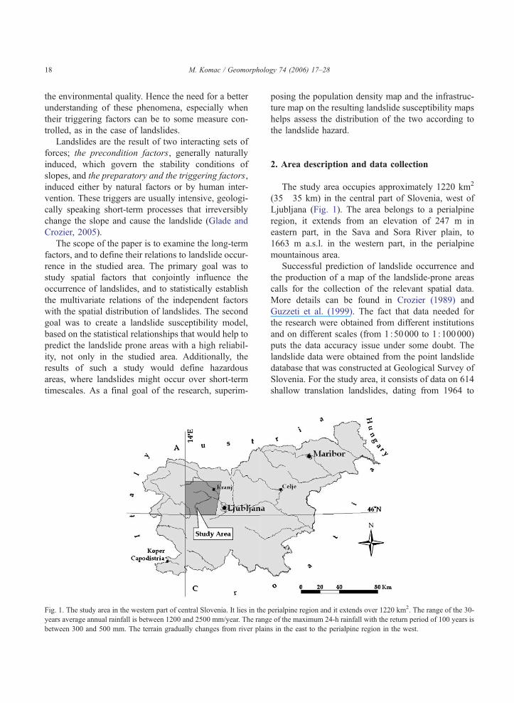
Fig. 1. The study area in the western part of central Slovenia. It lies in the

years average annual rainfall is between 1200 and 2500 mm/year. The rang

between 300 and 500 mm. The terrain gradually changes from river plain

posing the population density map and the infrastruc-

ture map on the resulting landslide susceptibility maps

helps assess the distribution of the two according to

the landslide hazard.

2. Area description and data collection

The study area occupies approximately 1220 km2

(35�35 km) in the central part of Slovenia, west of

Ljubljana (Fig. 1). The area belongs to a perialpine

region, it extends from an elevation of 247 m in

eastern part, in the Sava and Sora River plain, to

1663 m a.s.l. in the western part, in the perialpine

mountainous area.

Successful prediction of landslide occurrence and

the production of a map of the landslide-prone areas

calls for the collection of the relevant spatial data.

More details can be found in Crozier (1989) and

Guzzeti et al. (1999). The fact that data needed for

the research were obtained from different institutions

and on different scales (from 1 :50000 to 1 :100000)

puts the data accuracy issue under some doubt. The

landslide data were obtained from the point landslide

database that was constructed at Geological Survey of

Slovenia. For the study area, it consists of data on 614

shallow translation landslides, dating from 1964 to

perialpine region and it extends over 1220 km2. The range of the 30-

e of the maximum 24-h rainfall with the return period of 100 years is

s in the east to the perialpine region in the west.

M. Komac / Geomorphology 74 (2006) 17–28 19

2001. In the database landslides were classified into

four types; fossil or remnant landslides (68), dormant

landslides (413), creeping (57), and slides (60).

Approximate velocity equivalents (after Glade and

Crozier, 2005) for the four types are extremely slow,

very slow, slow, and very to extremely fast, respec-

tively. Sixteen landslides were classified as unknown

type. The digital elevation model (DEM) data were

obtained from the national 25 m resolution InSAR

DEM 25 (Survey and Mapping Administration,

2000a). All the additional data on the terrain morphol-

ogy (terrain curvature, elevation, slope, aspect, basins,

and primary slope-units) were derived from the DEM.

The bBasic Geological Map of Yugoslavia at the scale

of 1 :100000Q served as a source for the geological

data (Buser et al., 1967; Buser, 1968, 1987; Grad and

Ferjancic, 1974). For the land use and the vegetation

cover (cover type) reconnaissance, satellite images

from two different satellites were used and combined,

using a PCA (Principal Component Analysis) merging

method as explained in the next section. The multi-

spectral part of the satellite data was obtained from the

Landsat-5 TM images, and the high-resolution part

was obtained from the Resurs-F2 MK-4 images. The

topographic map at a scale of 1 :50000 was used as a

source of the surface water data (Survey and Mapping

Administration, 1994). The population density data

were obtained from National Office of Spatial Plan-

ning and Survey and Mapping Administration (1997)

and infrastructure data from Survey and Mapping

Administration (2000b). In the research area there

are around 135000 inhabitants and over 12000 km

of roads.

3. Methods

3.1. Satellite data

The multi-spectral satellite data, obtained from the

Landsat-5 TM images, were merged with the high-

resolution satellite data, obtained from the Resurs-F2

MK-4 images, using the principal component analysis

(PCA) joining method (Cliche et al., 1985; Chavez et

al., 1991; Sanjeevi et al., 2001; Vani et al., 2001).

Principal component analysis is a linear dimensional-

ity reduction technique, which identifies orthogonal

directions of maximum variance in the original data,

and projects the data into a lower-dimensionality

space formed of a sub-set of the highest-variance

components (Bishop, 1995). The principle of the

PCA joining method is that the first principal compo-

nent derived from the multi-spectral satellite data,

which relates to the data on surface albedo, is replaced

with the first principal component of the high-resolu-

tion satellite data, which also relates to the data on

surface albedo, but at a higher resolution. After the

merge, the principal components of multi-spectral

satellite data are retransformed back into the original

images but with a resolution of the high-resolution

images. Prior to the landslide susceptibility assess-

ment, the landslide population was split into the learn-

ing (293 landslides) and the testing sets (321

landslides) based on the temporal distribution of the

landslide population. The relation between the two is

not an ideal one, but the temporal boundary was

defined by the date of the acquisition of the satellite

images in September 1993. Since the learning set of

landslides, used in the susceptibility model develop-

ment, had to be bvisibleQ on the satellite images, the

landslides that occurred after the image acquisition

could not be used as a learning set. Next, all joined

images were classified according to landslide suscept-

ibility rate (areas or cover-types where more land-

slides have occurred have a higher possibility of

future landslide occurrence) using either the unsuper-

vised classification or the advanced red-green-blue

(RGB) clustering method (ERDAS, 1999), which

works better on spherically clustered data. The RGB

clustering method was used only on the images that

were transformed from orthogonal RGB colour model

to spherical CIE L*a*b* colour model (CIE, 1986).

Each of the 418 different colour composites was

classified into 1024 classes that were tested for land-

slide occurrence using Classification Success Index

(Komac, 2005). Based on the results of the v2 test for

their landslide susceptibility the 1024 classes of the

best colour composite were finally merged into 33

classes of different cover types that actually represent

different landslide susceptibilities.

3.2. Statistical analyses

To efficiently, and with lower costs, identify the

landslide-prone areas a better and more precise under-

standing of the relationship between the spatial factors

M. Komac / Geomorphology 74 (2006) 17–2820

is necessary. Carrara (1983) and Carrara et al. (1991)

have shown that statistical analyses of contributing

spatial factors can be successfully used for predicting

landslide prone areas. First, individual spatial factors

for the different landslide types and for landslides

generally, were tested with various statistical tests.

The Kolmogorov–Smirnov test and v2 test were

used for categorical and continuous variables (lithol-

ogy, cover type, slope inclination (slope), elevation,

aspect, terrain curvature, distance to geological

boundaries, distance to structural elements, and dis-

tance to rivers) and Student’s t test was used for the

continuous variables (the same variables as above,

except for lithology and the cover type). The confi-

dence limits of the analyses were set to 95%. The

univariate analyses were done on the whole landslide

population to determine the significance of each factor

for landslide susceptibility.

For the purpose of multivariate analyses, the learn-

ing set of landslides was randomly chosen from the

landslide population (394 or 64.2% of landslides with

similar portions for each landslide type) disregarding

the temporal component. Here the learning set is

almost twice as big as the testing set. Such a relation

between the learning and the testing set enables more

representative analytical results.

Multiple relations between the factors and the land-

slide distribution were tested with factor analysis (FA)

and multiple regression analysis (MRA). The impor-

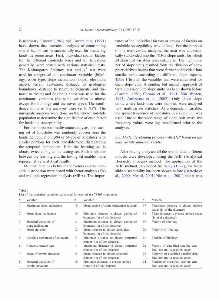
Table 1

List of the statistical variables, calculated for each of the 78365 slope un

# Variable # Variable

1 Maximum slope inclination 9 Mean cosine of slope or

2 Mean slope inclination 10 Minimum distance to c

boundary (ln of the dist

3 Standard deviation of

slope inclination

11 Maximum distance to c

boundary (ln of the dist

4 Mean elevation 12 Mean distance to closes

boundary (ln of the dist

5 Absolute maximum of curvature 13 Minimum distance to

element (ln of the distan

6 Convex/concave type 14 Maximum distance to

element (ln of the distan

7 Mean of terrain curvature 15 Mean distance to closes

element (ln of the distan

8 Standard deviation of

terrain curvature

16 Minimum distance to cl

water (ln of the distance

tance of the individual factors or groups of factors on

landslide susceptibility was defined. For the purpose

of the multivariate analysis, the area was automati-

cally subdivided into the 78365 slope units, for which

24 statistical variables were calculated. The high num-

ber of slope units resulted from the division of com-

puter-derived basins that were further subdivided into

smaller units according to different slope aspects.

Table 1 lists all the variables that were calculated for

each slope unit. A similar, but manual approach of

terrain division into slope units has been shown before

(Carrara, 1983; Carrara et al., 1991; Van Westen,

1993; Ardizzone et al., 2002). Only those slope

units, where landslides were mapped, were analysed

with multivariate statistics. As a dependant variable,

the spatial frequency of landslides in a slope unit was

used. Due to the wide range of slope unit areas, the

frequency values were log transformed prior to the

analyses.

3.3. Model developing process with AHP based on the

multivariate analyses results

After having analysed all the spatial data, different

models were developed, using the AHP (Analytical

Hierarchy Process) method. The application of the

AHP method, developed by Saaty (1977), for land-

slide susceptibility has been shown before (Barredo et

al., 2000; Mwasi, 2001; Nie et al., 2001) and it was

its

# Variable

ientation (aspect) 17 Maximum distance to closest surface

water (ln of the distance)

losest geological

ance)

18 Mean distance to closest surface water

(ln of the distance)

losest geological

ance)

19 Variety of lithology

t geological

ance)

20 Majority of lithology

closest structural

ce)

21 Median of lithology

closest structural

ce)

22 Variety of classified satellite data —

land use and vegetation cover

t structural

ce)

23 Majority of classified satellite data —

land use and vegetation cover

osest surface

)

24 Median of classified satellite data —

land use and vegetation cover

M. Komac / Geomorphology 74 (2006) 17–28 21

used to define the factors that govern landslide occur-

rence more transparently and to derive their weights.

For the model development, the results from the

multivariate analyses, both MRA and FA, were

used. One set of the models was developed using

the values from the statistics to manually define the

relationships between the different factors according

to the AHP methodology. These values were later

imported into the AHP matrixes. The other set of

the models was developed by automatically importing

the calculated relationship values between different

factors, based on the statistical values, into the AHP

matrixes. For all the models, where AHP was used,

the CR (Consistency Ratio) was calculated (see Saaty,

1977). The models with the CR greater than 0.1 were

automatically rejected. With the AHP method, the

values of spatial factors weights were defined. Using

a weighted linear sum procedure (Voogd, 1983) the

acquired weights were used to calculate the landslide

susceptibility models.

To effectively compare the calculated models, the

normalisation of the results had to be done. Taking

into account the normal distribution of the results, an

approximation was done, where in each of the model,

the highest value represented the highest landslide

susceptibility, and the lowest value represented the

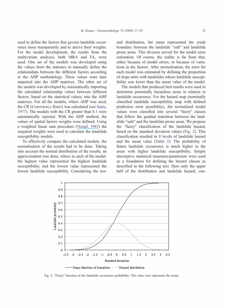
lowest landslide susceptibility. Considering the nor-

Fig. 2. bFuzzyQ function of the landslide occurrence p

mal distribution, the mean represented the crude

boundary between the landslide bsafeQ and landslide

prone areas. This division served for the model error

estimation. Of course, the reality is far from that,

either because of model errors, or because of varia-

tions in the factors. After normalisation, the error for

each model was estimated by defining the proportion

of slope units with landslides whose landslide suscept-

ibility was lower than the mean value of the model.

The models that produced best results were used to

determine potentially hazardous areas in relation to

landslide occurrence. For the hazard map (nominally

classified landslide susceptibility map with defined

prediction error possibility), the normalised model

values were classified into several bfuzzyQ classes

that follow the gradual transition between the land-

slide-bsafeQ and the landslide-prone areas. We propose

the bfuzzyQ classification of the landslide hazard,

based on the standard deviation values (Fig. 2). This

classification resulted in 8 levels of landslide hazard

and the mean value (Table 2). The probability of

future landslide occurrence is much higher in the

areas with higher landslide susceptibility. Simple

descriptive statistical measures/parameters were used

as a foundation for defining the hazard classes as

described in the following text. Here only the upper

half of the distribution and landslide hazard, con-

robability. The value zero represents the mean.

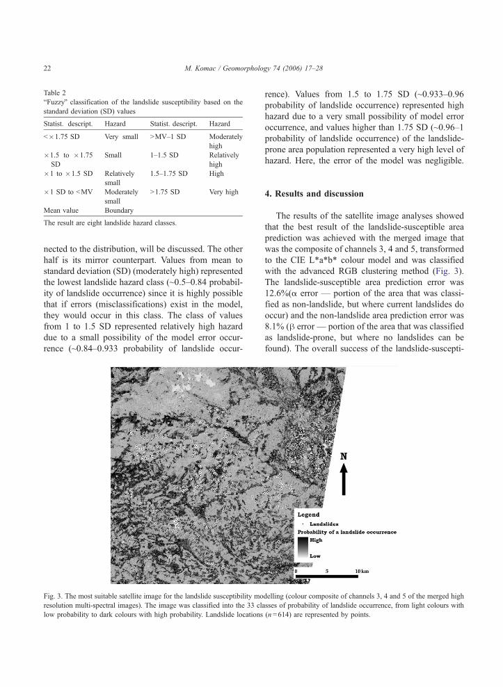
Table 2

bFuzzyQ classification of the landslide susceptibility based on the

standard deviation (SD) values

Statist. descript. Hazard Statist. descript. Hazard

b�1.75 SD Very small NMV–1 SD Moderately

high

�1.5 to �1.75

SD

Small 1–1.5 SD Relatively

high

�1 to �1.5 SD Relatively

small

1.5–1.75 SD High

�1 SD to bMV Moderately

small

N1.75 SD Very high

Mean value Boundary

The result are eight landslide hazard classes.

M. Komac / Geomorphology 74 (2006) 17–2822

nected to the distribution, will be discussed. The other

half is its mirror counterpart. Values from mean to

standard deviation (SD) (moderately high) represented

the lowest landslide hazard class (~0.5–0.84 probabil-

ity of landslide occurrence) since it is highly possible

that if errors (misclassifications) exist in the model,

they would occur in this class. The class of values

from 1 to 1.5 SD represented relatively high hazard

due to a small possibility of the model error occur-

rence (~0.84–0.933 probability of landslide occur-

Fig. 3. The most suitable satellite image for the landslide susceptibility mo

resolution multi-spectral images). The image was classified into the 33 cl

low probability to dark colours with high probability. Landslide locations

rence). Values from 1.5 to 1.75 SD (~0.933–0.96

probability of landslide occurrence) represented high

hazard due to a very small possibility of model error

occurrence, and values higher than 1.75 SD (~0.96–1

probability of landslide occurrence) of the landslide-

prone area population represented a very high level of

hazard. Here, the error of the model was negligible.

4. Results and discussion

The results of the satellite image analyses showed

that the best result of the landslide-susceptible area

prediction was achieved with the merged image that

was the composite of channels 3, 4 and 5, transformed

to the CIE L*a*b* colour model and was classified

with the advanced RGB clustering method (Fig. 3).

The landslide-susceptible area prediction error was

12.6%(a error — portion of the area that was classi-

fied as non-landslide, but where current landslides do

occur) and the non-landslide area prediction error was

8.1% (h error — portion of the area that was classified

as landslide-prone, but where no landslides can be

found). The overall success of the landslide-suscepti-

delling (colour composite of channels 3, 4 and 5 of the merged high

asses of probability of landslide occurrence, from light colours with

(n =614) are represented by points.

M. Komac / Geomorphology 74 (2006) 17–28 23

ble area classification of the best model was 79.2%.

The result represents the classification of the vegeta-

tion/land-use type (cover type) according to landslide

susceptibility and does not deal with vegetation or

land-use types. The merged multi-spectral high-reso-

lution satellite images proved to convey useful infor-

mation on landslide occurrence, without having

detailed knowledge about the land cover type of the

terrain under investigation.

The univariate analyses results showed that the

following factors proved to play an important role

(in brackets the significance classes are given): the

slope (N148), the terrain curvature (concave from �2

to �0.5), the distance to the geological boundaries

(2.5–50 m), the distance to rivers (7.5–150 m), the

lithology (shale; scree deposits; graywacke, sand-

stone, shale, marly shale, and tuff; sandstone, shale,

siltstone, conglomerate, and marl; sandstone, argillite,

and tuff; pyroclastites), and the cover type (not

defined, since the type was not assessed). The slopes

above 148 tend to be much more unstable than the less

steep ones, although analyses have also shown that

also the class from 118 to 148 tends to be very

unstable, especially in looser materials (gravel and

sand). The terrain curvature indicates that landslides

tend to occur in concave areas where the concentra-

tion of pore water is higher. Closeness of landslide

occurrence to geological boundaries might be the

consequence of the contacts between overlying more

and underlying less permeable rocks resulting in

abundance of springs and hence more soil moisture,

or the consequence of the difference in behaviour in

case of the earthquakes. The distance to rivers clearly

indicates two possible reasons. One is the presence of

Table 3

Proportions of the variance, explained by factor loadings (factor analysis

All landslides Fossil landslides Dormant

F1 1, 2, 5 & 8 (22%) 3, 20 & 21 (26%) 1, 2, 3, 5

F2 20 & 21 (15%) 1, 2 & 8 (19%) 18 & 22

F3 7 & 18 (12%) 7 & 22 (12%) 9, 23 &

F4 9, 23 & 24 (10%) 15 & 19 (9%) 20 & 21

F5 19 & 22 (7.5%) 23 & 24 (8%) 15 (8%)

F6 15 (6%) 18 (7%) 6 (6%)

F7 6 (5.5%) – 12 & 19

Sum 78.3% 80.2% 79.2%

Numbers in fields represent the variables, listed in the Table 1. In brackets t

given. The first column represents factors and the last row represents the s

the landslides and for each landslide type.

groundwater, and the other is the undercutting process

by running surface waters. Considering lithological

units, landslide occurrence is expected in the litholo-

gical units, given above, due to their geomechanical

properties, either due to the friction angles or due to

the presence of pore water.

Comparing the results of multivariate analyses, the

FA (principal component) proved to be the most appro-

priate and reliable method for landslide susceptibility

assessment. Table 3 shows the proportions of the var-

iance, explained by various factors that are represented

by one or more variables. Each individual variable is

numbered and its description is explained in Table 1.

At the bottom, the total explained variance is shown.

The explained variance values indicate that the factors

chosen for the landslide susceptibility analyses repre-

sent around 80% of landslide occurrence governing

factors. In other words, these results may suggest that

precondition factors represent roughly 80%, and the

preparatory and the triggering factors represent the rest

of the influence on landslide occurrence.

Table 4 shows the values for the weights for the

spatial factors in the most suitable susceptibility mod-

els for different landslide types. The last row shows

the error for each of the models. For all types of

landslides the susceptibility models developed with

the FA gave the best results, except for slides where

the MRA model achieved the same success rate as the

FA model. The best susceptibility model for all land-

slides (n =614) showed that the most important pre-

condition factors were the lithological properties

(36.5%), followed by the slope (21.2%), the cover

type properties (17.6%), the terrain roughness

(10.1%), the terrain curvature (8.6%), the distance to

— principal component method)

landslides Creeping Slides

& 8 (24%) 20 & 21 (23%) 1, 2, 3, 5 & 8 (27%)

(14%) 1, 2, 5 & 8 (19%) 6, 12 & 19 (16%)

24 (12%) 7 & 18 (15%) 20 & 21 (14%)

(10%) 9, 23 & 24 (12%) 23 & 24 (10%)

15 & 19 (6.5%) 7 (7.5%)

6 (5.5%) 15 (6%)

(5.5%) – –

80.4% 80.5%

he proportion of the explained variance by variables in given field is

um of the explained variance of the best susceptibility model for all

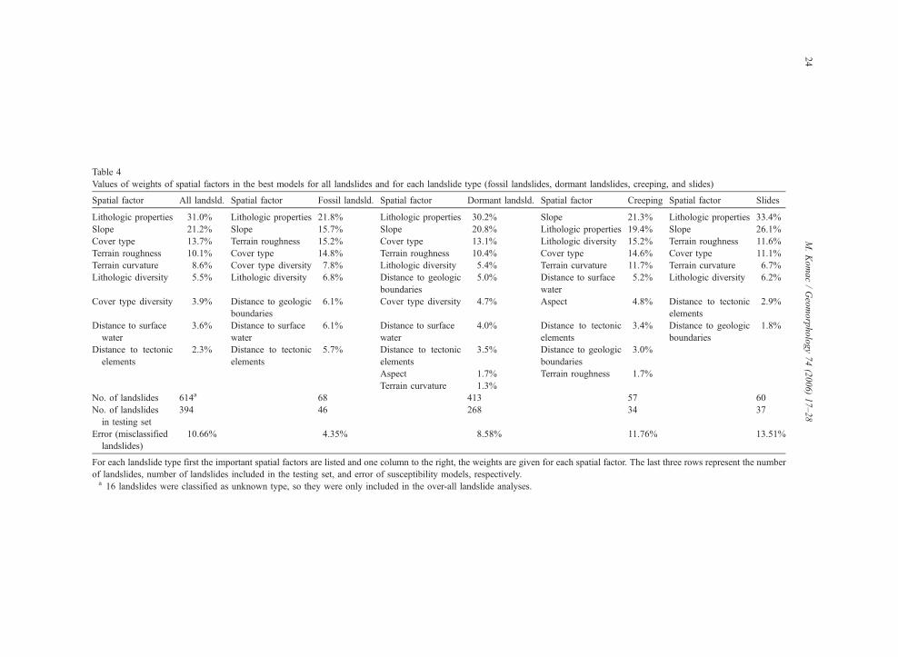
Table 4

Values of weights of spatial factors in the best models for all landslides and for each landslide type (fossil landslides, dormant landslides, creeping, and slides)

Spatial factor All landsld. Spatial factor Fossil landsld. Spatial factor Dormant landsld. Spatial factor Creeping Spatial factor Slides

Lithologic properties 31.0% Lithologic properties 21.8% Lithologic properties 30.2% Slope 21.3% Lithologic properties 33.4%

Slope 21.2% Slope 15.7% Slope 20.8% Lithologic properties 19.4% Slope 26.1%

Cover type 13.7% Terrain roughness 15.2% Cover type 13.1% Lithologic diversity 15.2% Terrain roughness 11.6%

Terrain roughness 10.1% Cover type 14.8% Terrain roughness 10.4% Cover type 14.6% Cover type 11.1%

Terrain curvature 8.6% Cover type diversity 7.8% Lithologic diversity 5.4% Terrain curvature 11.7% Terrain curvature 6.7%

Lithologic diversity 5.5% Lithologic diversity 6.8% Distance to geologic

boundaries

5.0% Distance to surface

water

5.2% Lithologic diversity 6.2%

Cover type diversity 3.9% Distance to geologic

boundaries

6.1% Cover type diversity 4.7% Aspect 4.8% Distance to tectonic

elements

2.9%

Distance to surface

water

3.6% Distance to surface

water

6.1% Distance to surface

water

4.0% Distance to tectonic

elements

3.4% Distance to geologic

boundaries

1.8%

Distance to tectonic

elements

2.3% Distance to tectonic

elements

5.7% Distance to tectonic

elements

3.5% Distance to geologic

boundaries

3.0%

Aspect 1.7% Terrain roughness 1.7%

Terrain curvature 1.3%

No. of landslides 614a 68 413 57 60

No. of landslides

in testing set

394 46 268 34 37

Error (misclassified

landslides)

10.66% 4.35% 8.58% 11.76% 13.51%

For each landslide type first the important spatial factors are listed and one column to the right, the weights are given for each spatial factor. The last three rows represent the number

of landslides, number of landslides included in the testing set, and error of susceptibility models, respectively.a 16 landslides were classified as unknown type, so they were only included in the over-all landslide analyses.

M.Komac/Geomorphology74(2006)17–28

24

M. Komac / Geomorphology 74 (2006) 17–28 25

surface waters (3.6%), and the distance to tectonic

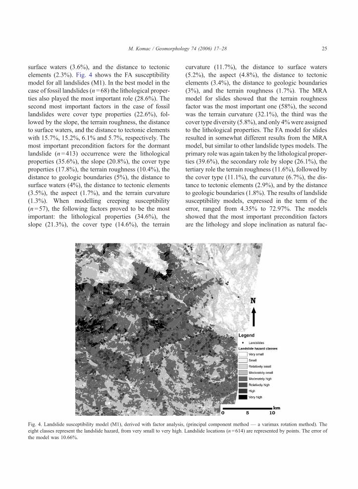
elements (2.3%). Fig. 4 shows the FA susceptibility

model for all landslides (M1). In the best model in the

case of fossil landslides (n =68) the lithological proper-

ties also played the most important role (28.6%). The

second most important factors in the case of fossil

landslides were cover type properties (22.6%), fol-

lowed by the slope, the terrain roughness, the distance

to surface waters, and the distance to tectonic elements

with 15.7%, 15.2%, 6.1% and 5.7%, respectively. The

most important precondition factors for the dormant

landslide (n =413) occurrence were the lithological

properties (35.6%), the slope (20.8%), the cover type

properties (17.8%), the terrain roughness (10.4%), the

distance to geologic boundaries (5%), the distance to

surface waters (4%), the distance to tectonic elements

(3.5%), the aspect (1.7%), and the terrain curvature

(1.3%). When modelling creeping susceptibility

(n =57), the following factors proved to be the most

important: the lithological properties (34.6%), the

slope (21.3%), the cover type (14.6%), the terrain

Fig. 4. Landslide susceptibility model (M1), derived with factor analysis,

eight classes represent the landslide hazard, from very small to very high.

the model was 10.66%.

curvature (11.7%), the distance to surface waters

(5.2%), the aspect (4.8%), the distance to tectonic

elements (3.4%), the distance to geologic boundaries

(3%), and the terrain roughness (1.7%). The MRA

model for slides showed that the terrain roughness

factor was the most important one (58%), the second

was the terrain curvature (32.1%), the third was the

cover type diversity (5.8%), and only 4%were assigned

to the lithological properties. The FA model for slides

resulted in somewhat different results from the MRA

model, but similar to other landslide types models. The

primary role was again taken by the lithological proper-

ties (39.6%), the secondary role by slope (26.1%), the

tertiary role the terrain roughness (11.6%), followed by

the cover type (11.1%), the curvature (6.7%), the dis-

tance to tectonic elements (2.9%), and by the distance

to geologic boundaries (1.8%). The results of landslide

susceptibility models, expressed in the term of the

error, ranged from 4.35% to 72.97%. The models

showed that the most important precondition factors

are the lithology and slope inclination as natural fac-

(principal component method — a varimax rotation method). The

Landslide locations (n =614) are represented by points. The error of

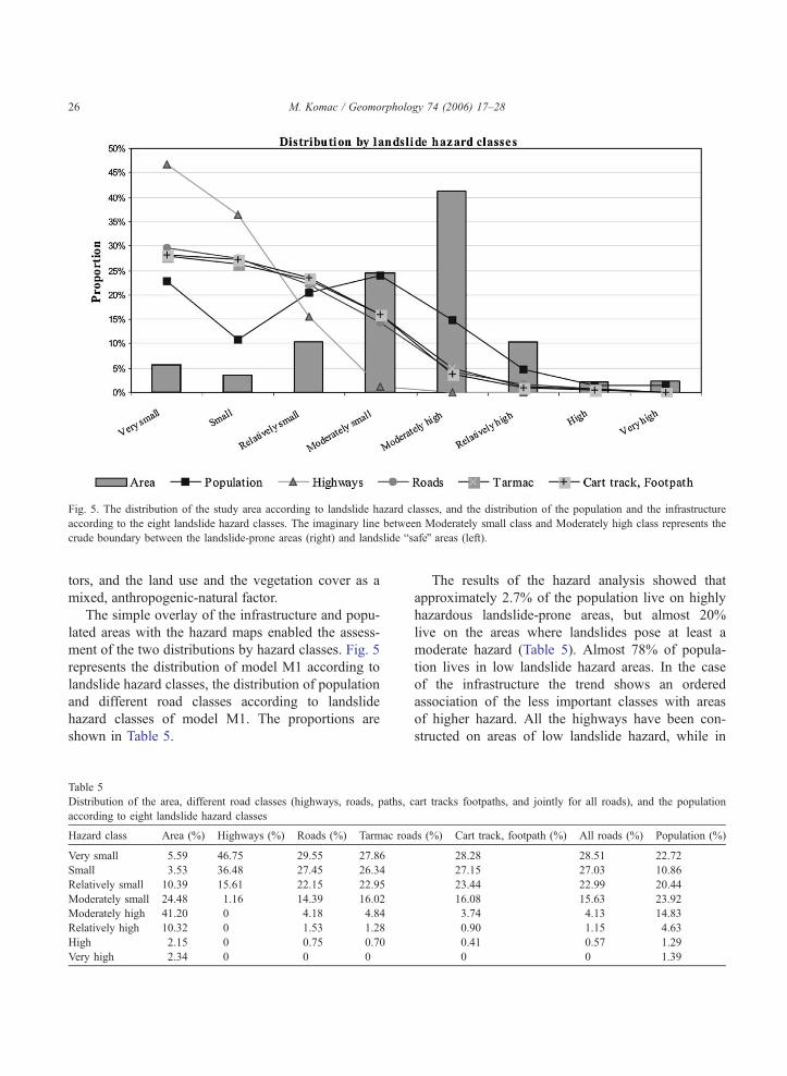
Fig. 5. The distribution of the study area according to landslide hazard classes, and the distribution of the population and the infrastructure

according to the eight landslide hazard classes. The imaginary line between Moderately small class and Moderately high class represents the

crude boundary between the landslide-prone areas (right) and landslide bsafeQ areas (left).

M. Komac / Geomorphology 74 (2006) 17–2826

tors, and the land use and the vegetation cover as a

mixed, anthropogenic-natural factor.

The simple overlay of the infrastructure and popu-

lated areas with the hazard maps enabled the assess-

ment of the two distributions by hazard classes. Fig. 5

represents the distribution of model M1 according to

landslide hazard classes, the distribution of population

and different road classes according to landslide

hazard classes of model M1. The proportions are

shown in Table 5.

Table 5

Distribution of the area, different road classes (highways, roads, paths, c

according to eight landslide hazard classes

Hazard class Area (%) Highways (%) Roads (%) Tarmac roa

Very small 5.59 46.75 29.55 27.86

Small 3.53 36.48 27.45 26.34

Relatively small 10.39 15.61 22.15 22.95

Moderately small 24.48 1.16 14.39 16.02

Moderately high 41.20 0 4.18 4.84

Relatively high 10.32 0 1.53 1.28

High 2.15 0 0.75 0.70

Very high 2.34 0 0 0

The results of the hazard analysis showed that

approximately 2.7% of the population live on highly

hazardous landslide-prone areas, but almost 20%

live on the areas where landslides pose at least a

moderate hazard (Table 5). Almost 78% of popula-

tion lives in low landslide hazard areas. In the case

of the infrastructure the trend shows an ordered

association of the less important classes with areas

of higher hazard. All the highways have been con-

structed on areas of low landslide hazard, while in

art tracks footpaths, and jointly for all roads), and the population

ds (%) Cart track, footpath (%) All roads (%) Population (%)

28.28 28.51 22.72

27.15 27.03 10.86

23.44 22.99 20.44

16.08 15.63 23.92

3.74 4.13 14.83

0.90 1.15 4.63

0.41 0.57 1.29

0 0 1.39

M. Komac / Geomorphology 74 (2006) 17–28 27

the case of other tarmac roads less than 1% lie in

the areas of high landslide hazard, and around 6.5%

in the areas with at least a moderate landslide

hazard. Just over 5% of cart tracks and footpaths

lie in the areas with at least a moderate landslide

hazard, and less than 0.5% in areas of high land-

slide hazard.

5. Conclusions

Landslide occurrence and behaviour are governed

by numerous spatial factors that can be, for the

purpose of regional susceptibility assessment, cut

down to several important ones. These factors can

be relatively easily acquired from geological maps,

topographic maps, DEMs, and satellite imagery.

Using these data, good landslide susceptibility mod-

els were developed. It has been shown that using

merged multi-spectral high-resolution satellite images

landslide-prone areas can be effectively defined and

later used for landslide susceptibility model develop-

ment. The results of the univariate statistics proved

to be useful in assessing the importance of each

individual factor. The univariate statistics results

have indicated the same important factors as the

multivariate analyses, but they cannot be simply

used for susceptibility model development, since

neglecting the existing interactions between factors

results in wrong predictions. Multivariate statistics

were used instead and factor analysis proved to be

the most effective multivariate statistical tool in

developing a landslide susceptibility model. It has

been shown that the use of the AHP method gives a

mean to define the factor weights in the linear land-

slide susceptibility model. Based on simple descrip-

tive statistical measures like standard deviation and

occurrence probability, hazard maps were derived

from susceptibility maps. Unfortunately the fre-

quency of the triggering event could not be deter-

mined due to insufficient data hence the frequency of

landslide occurrence could not be clearly defined. It

is not clear whether the high number of landslides

that occurred after September 1993 in comparison to

those that occurred before indicates that the occur-

rence frequency is growing or that the high number

is simply the result of a more systematic approach to

landslide mapping.

References

Ardizzone, F., Cardinali, M., Carrara, A., Guzzeti, F., Reichen-

bach, P., 2002. Impact of mapping errors on the reliability of

landslide hazard maps. Natural Hazards and Earth System

Sciences 2, 3–14.

Barredo, J.I., Benavides, A., Hervas, J., Van Westen, C.J., 2000.

Comparing heuristic landslide hazard assessment techniques

using GIS in the Tirajana basin, Gran Canaria Island, Spain.

International Journal of Applied Earth Observation and Geoin-

formation 2, 9–23.

BBC, 2002. Floods Wreak Havoc in Germany. (http://news.

bbc.co.uk/2/hi/europe/2194395.stm, 28th June, 2005).

Bishop, C., 1995. Neural Networks for Pattern Recognition. Uni-

versity Press, Oxford.

Buser, S., 1968. Osnovna geoloska karta SFRJ, lista Gorica,

1 :100,000=basic geological map of Yugoslavia, Map Gorica,

scale 1 :100,000. Zvezni geoloski zavod, Belgrade.

Buser, S., 1987. Osnovna geoloska karta SFRJ, list Tolmin in

Videm, 1 :100,000=basic geological map of Yugoslavia, Map

Tolmin and Udine, scale 1 :100,000. Zvezni geoloski zavod,

Belgrade.

Buser, S., Grad, K., Pleniar, M. 1967. Osnovna geoloska karta

SFRJ, list Postojna, 1 :100,000=basic geological map of Yugo-

slavia, Map Postojna, scale 1 :100,000. Zvezni geoloski zavod,

Belgrade.

Carrara, A., 1983. Multivariate models for landslide hazard evalua-

tion. Mathematical Geology 15, 403–426.

Carrara, A., Cardinali, M., Detti, R., Guzzetti, F., Pasqui, V., Reich-

enbach, P., 1991. GIS techniques and statistical models in

evaluating landslide hazard. Earth Surface Processes and Land-

forms 16, 427–445.

Chavez Jr., P.S., Slides, S.C., Anderson, J.A., 1991. Comparison

three different methods to merge multiresolution and multispec-

tral data: Landsat TM and SPOT panchromatic. Photogram-

metric Engineering and Remote Sensing 57, 295–303.

CIE, 1986. Colorimetry, Second edition. Commission Internationale

de L’Eclarirage, Paris.

Cliche, G., Bonn, F., Teillet, P., 1985. Integration of the SPOT pan

channel into its multispectral mode for image sharpness

enhancement. Photogrammetric Engineering and Remote Sen-

sing 51, 311–316.

Crozier, M.J., 1989. Landslides: Causes, Consequences and Envir-

onment. Routledge, London.

ERDAS, 1999. ERDAS Field Guide. ERDAS, Inc., Atlanta.

Glade, T., Crozier, M.J., 2005. The nature of landslide hazard impact.

In: Glade, T., Anderson, M.G., Crozier, M.J. (Eds.), Landslide

Hazard and Risk. Wiley, Chichester, pp. 43–74.

Grad, K., Ferjancic, L., 1974. Osnovna geoloska karta SFRJ, list

Kranj, 1 :100,000=basic geological map of Yugoslavia, Map

Kranj, scale 1 :100,000. Zvezni geoloski zavod, Belgrade.

Guzzeti, F., Carrara, A., Cardinali, M., Reichenbach, P., 1999.

Landslide hazard evaluation: a review of current techniques

and their application in a multi-scale study, central Italy. Geo-

morphology 31, 181–216.

Komac, M., 2005. Napoved verjetnosti pojavljanja plazov z analizo

satelitskih in drugih prostorskih podatkov (Landslide occurrence

M. Komac / Geomorphology 74 (2006) 17–2828

prediction with analysis of satellite images and other spatial

data). Geological Survey of Slovenia, Ljubljana, pp. 136–138.

Mwasi, B., 2001. Land use conflicts resolution in a fragile ecosys-

tem using Multi-Criteria Evaluation (MCE) and a GIS-based

Decision Support System (DSS). Int. Conf. on Spatial Informa-

tion for Sustainable Development, Nairobi, Kenya, FIG —

International Federation of Surveyors. 11 pp.

National Office of Spatial Planning and Survey and Mapping

Administration, 1997. Population density per hectare by classes.

Database 1,28 MB, Ljubljana.

Nie, H.F., Diao, S.J., Liu, J.X., Huang, H., 2001. The application of

remote sensing technique and AHP-fuzzy method in compre-

hensive analysis and assessment for regional stability of

Chongqing City, China. Proc. of the 22nd Asian Conf. on

Remote Sensing, Vol. 1, Centre for Remote Imaging, Sensing

and Processing (CRISP), National University of Singapore,

Singapore Institute of Sorveyors and Valuers (SISV) and

Asian Association on Remote Sensing (AARS), Singapore,

pp. 660–665.

Saaty, T.L., 1977. A scaling method for priorities in hierarchical

structures. Journal of Mathematical Psychology 15, 234–281.

Sanjeevi, S., Vani, S., Lakshmi, K., 2001. Comparison of conven-

tional and wavelet transformation techniques for fusion of IRS-

1C LISS-III and PAN images. Proc. of the 22nd Asian Conf. on

Remote Sensing, Vol. 1, Centre for Remote Imaging, Sensing

and Processing (CRISP), National University of Singapore,

Singapore Institute of Sorveyors and Valuers (SISV) and

Asian Association on Remote Sensing (AARS), Singapore,

pp. 140–145.

Survey and Mapping Administration, 1994. Skanogrami TK 50 —

topografske karte merila 1 :50,000. Datum vira: 1978–

1987=TK 50 — topographic maps at scale 1 :50,000, acquisi-

tion date 1978–1987. Geodetska uprava Republike Slovenije,

Ljubljana.

Survey and Mapping Administration, 2000a. InSAR DMV 25

(digitalni model visin)= InSAR DEM 25 (digital elevation

model). Geodetska uprava Republike Slovenije, Ljubljana.

Survey and Mapping Administration, 2000b. Generalizirana karto-

grafska baza v M 1:25,000—ceste. Datum vira: 1994–

2000=generalised cartographic database, scale 1 :25,000 —

roads, acquisition date 1994–2000. Geodetska uprava Republike

Slovenije, Ljubljana.

Van Westen, C.J., 1993. GISSIZ — training package for geographic

information systems in slope instability zonation. Theory, vol. 1.

ITC, Enschede.

Vani, K., Shanmugavel, S., Marruthachalam, M., 2001. Fusion of

IRS-LISS and pan images using different resolution ratios. Proc.

of the 22nd Asian Conf. on Remote Sensing, Vol. 1, Centre for

Remote Imaging, Sensing and Processing (CRISP), National

University of Singapore, Singapore Institute of Sorveyors and

Valuers (SISV) and Asian Association on Remote Sensing

(AARS), Singapore, pp. 146–151.

Voogd, H., 1983. Multicriteria Evaluation for Urban and Regional

Planning. Pion Ltd., London.