econstorMake Your Publications Visible.

A Service of

zbwLeibniz-InformationszentrumWirtschaftLeibniz Information Centrefor Economics

Jobst, Andreas A.

Working Paper

European Securitisation: A GARCH Model of CDO,MBS and Pfandbrief Spreads

Working Paper Series: Finance & Accounting, No. 121

Provided in Cooperation with:Faculty of Economics and Business Administration, Goethe University Frankfurt

Suggested Citation: Jobst, Andreas A. (2003) : European Securitisation: A GARCHModel of CDO, MBS and Pfandbrief Spreads, Working Paper Series: Finance &Accounting, No. 121, Johann Wolfgang Goethe-Universität Frankfurt am Main, FachbereichWirtschaftswissenschaften, Frankfurt a. M.,http://nbn-resolving.de/urn:nbn:de:hebis:30-16119

This Version is available at:http://hdl.handle.net/10419/76885

Standard-Nutzungsbedingungen:

Die Dokumente auf EconStor dürfen zu eigenen wissenschaftlichenZwecken und zum Privatgebrauch gespeichert und kopiert werden.

Sie dürfen die Dokumente nicht für öffentliche oder kommerzielleZwecke vervielfältigen, öffentlich ausstellen, öffentlich zugänglichmachen, vertreiben oder anderweitig nutzen.

Sofern die Verfasser die Dokumente unter Open-Content-Lizenzen(insbesondere CC-Lizenzen) zur Verfügung gestellt haben sollten,gelten abweichend von diesen Nutzungsbedingungen die in der dortgenannten Lizenz gewährten Nutzungsrechte.

Terms of use:

Documents in EconStor may be saved and copied for yourpersonal and scholarly purposes.

You are not to copy documents for public or commercialpurposes, to exhibit the documents publicly, to make thempublicly available on the internet, or to distribute or otherwiseuse the documents in public.

If the documents have been made available under an OpenContent Licence (especially Creative Commons Licences), youmay exercise further usage rights as specified in the indicatedlicence.

www.econstor.eu

JOHANN WOLFGANG GOETHE-UNIVERSITÄT FRANKFURT AM MAIN

FACHBEREICH WIRTSCHAFTSWISSENSCHAFTEN

WORKING PAPER SERIES: FINANCE & ACCOUNTING

Andreas Jobst

European Securitisation:

A GARCH Model of CDO, MBS and Pfandbrief Spreads

No. 121

November 2003

European Securitisation: A GARCH Model of CDO, MBS and Pfandbrief Spreads

Andreas Jobst#

No. 121

November 2003

ISSN 1434-3401

Working Paper Series Finance and Accounting are intended to make research findings available to other researchers in preliminary form, to encourage discussion and suggestions for revision before final publication. Opinions are solely those of the authors.

# J.W. Goethe Universität Frankfurt am Main, Department of Finance, 60325 Frankfurt am Main, Germany, and Financial Markets Group (FMG), London School of Economics and Political Science (LSE), Houghton Street, London WC2A 2AE, England, U.K. e-mail: a.a.jobst@lse.ac.uk. This paper was completed in the course of a research project sponsored by the German Science Foundation (Deutsche Forschungsgemeinschaft) and the Center for Financial Studies (CFS).

European Securitisation:

A GARCH Model of CDO, MBS and Pfandbrief Spreads

Andreas Jobst#

Version: 21 December 2003

Abstract

Asset-backed securitisation (ABS) is an asset funding technique that involves the issuance of structured claims on the cash flow performance of a designated pool of underlying receivables. Efficient risk management and asset allocation in this growing segment of fixed income markets requires both investors and issuers to thoroughly understand the longitudinal properties of spread prices. We present a multi-factor GARCH process in order to model the heteroskedasticity of secondary market spreads for valuation and forecasting purposes. In particular, accounting for the variance of errors is instrumental in deriving more accurate estimators of time-varying forecast confidence intervals. On the basis of CDO, MBS and Pfandbrief transactions as the most important asset classes of off-balance sheet and on-balance sheet securitisation in Europe we find that expected spread changes for these asset classes tends to be level stationary with model estimates indicating asymmetric mean reversion. Furthermore, spread volatility (conditional variance) is found to follow an asymmetric stochastic process contingent on the value of past residuals. This ABS spread behaviour implies negative investor sentiment during cyclical downturns, which is likely to escape stationary approximation the longer this market situation lasts.

Keywords: Securitisation, MBS, CDO, CLO, CBO, ABS, Pfandbrief, GARCH model, structured finance JEL: C12, C32, C53, G12, G21

# J.W. Goethe Universität Frankfurt am Main, Department of Finance, 60325 Frankfurt am Main, Germany, and Financial Markets Group (FMG), London School of Economics and Political Science (LSE), Houghton Street, London WC2A 2AE, England, U.K. e-mail: a.a.jobst@lse.ac.uk. This paper was completed in the course of a research project sponsored by the German Science Foundation (Deutsche Forschungsgemeinschaft) and the Center for Financial Studies (CFS).

2

1 INTRODUCTION

1.1 Objective

Securitisation seeks to substitute capital market-based finance for credit finance by sponsoring financial

relationships without the lending and deposit-taking capabilities of banks (disintermediation). Generally,

securitisation represents a structured finance transaction, where receivables from a designated asset

portfolio are sold as contingent claims on cash flows from repayment in the bid to increase the issuer’s

liquidity position and to support a broadening of lending business (refinancing) without increasing the

capital base (funding motive). Aside from being a funding instrument, securitisation also serves (i) to reduce

both economic cost of capital and regulatory minimum capital requirements as a balance sheet

restructuring tool (regulatory and economic motive), (ii) to diversify asset exposures (especially interest rate risk

and currency risk) as issuers repackage receivables into securitisable asset pools (collateral) underlying the

so-called asset-backed securitisation (ABS) transactions (hedging motive). Also the generation of securitised cash

flows from a diversified asset portfolio represents an effective method of redistributing credit risks to

investors and broader capital markets. These issuer incentives correspond to a certain investment appetites

in ABS. As opposed to ordinary creditor claims in lending relationships, the liquidity of a securitised

contingent claim on a promised portfolio performance in an structured transaction affords investors at

low transaction costs to quickly adjust their investment holdings due to changes in personal risk

sensitivity, market sentiment and/or consumption preferences.

Asset-backed securitisation (ABS) represents a growing segment of European structured finance. Efficient

risk and asset allocation through seasoned trading in this relatively young fixed income market requires

both investors and issuers to thoroughly understand the longitudinal properties of spread prices (over

benchmark risk-free market interest rate) of traded securities, which reflect various risk factors of a

transaction. Spreads are closely watched by investors and issuers alike, and by doing so, they create an

efficient primary and secondary markets of informed investment. For loss of any technical study on

secondary pricing in structured finance markets outside the U.S., examining the spread development of

European structured transactions proves particularly interesting.

While recent research has generated essential information concerning the determination of ABS spreads

(Goodman and Ho, 1997 and 1998; Arora et al. (2000)), the time series properties of these structured

finance fixed income investments have been insufficiently addressed. Although research by Koutmos

(2001 and 2002) develops a model for the spread dynamics of U.S. MBS transactions, it falls short of

addressing other forms of ABS transactions (CDO) and quasi-ABS transactions (Pfandbriefe), with the

latter deal type easily matches U.S. MBS by any standard of comparison, be it market volume, trading

activity or historical track record.

3

In the following paper we conduct an empirical analysis of the spread change behaviour of European

MBS and CDO transactions as well as Pfandbriefe in order to verify previous studies about certain time

series properties of U.S. MBS spread data. Moreover, by using secondary market trading data of European

ABS transactions we expand the existing empirical horizon of previous time series analysis of structured

finance products. So far no study on the term structure of ABS spreads has been completed on European

secondary market trading data. We develop a technical pricing and forecasting approach for the estimation

of secondary market spreads of ABS transactions (and their constituent tranches) as a discrete

approximation of a multi-factor continuous time model. We enlist modified GARCH(1,1) and

GARCH(2,1) models in order to examine any volatility-induced future movements of logarithmic ABS

spreads, their degree of symmetry and time variation as well as the corresponding volatility process.

Hence, we aim to document the heteroskedasticity of ABS spread processes in order to learn about how

past volatility of ABS spreads and changes in the spot rate (LIBOR) explain spread dynamics. We extend

the approaches taken by Koutmos (2002) and Longstaff and Schwartz (1992) in order to find out whether

spread volatility is constant or time-varying and whether observed spreads support either the existence

and the dynamics of mean reversion or a random walk in level and first moment. Finally, we ensure the

practical usefulness of the presented model for spread forecasting purposes in a correct model

specification through various statistical diagnostics. The results could provide useful insights for adequate

secondary market pricing of ABS issues with varying credit quality and an efficient management of ABS

portfolios with respect to risk-return considerations.

The rest of the paper is organised as follows. In the subsequent section we examine selected statistical

diagnostics of linear regression analysis (normality assumption and autocorrelation) after all descriptive

statistics have been exhaustively analysed. In the next section, we discuss the effects of data

transformation on time series dynamics before we determine the presence of level stationarity as an

important requirement for simple hypothesis testing. In the subsequent section we crystallise in a number

of formal statements a GARCH(1,1) and a GARCH(2,1) process of the heteroskedasticity for the spread

series of CDO, MBS and Pfandbrief transactions. This is a necessary step to take in the process of

translating continuous time models of the term structure of interest rates into a approximate two-factor

model of spread dynamics. In the next section we present the estimation results of both GARCH models

and verify the correct model specification by means of residual and coefficient tests. Following that, we

discuss its econometric implications before we conclude in the last section.

1.2 Securitisation background

The flexible security design of asset-backed securitisation allows for a variety of asset types to be used ain

securitised reference portfolios. Mortgage-backed securities (MBS), real estate and non-real estate asset-backed

securities (ABS) and collateralised debt obligations (CDO) represent the three main strands of asset-backed

securitisation in a broader sense. All ABS structures engross different criteria of legal and economic

4

considerations, which all converge upon a basic distinction of security design: traditional vs. synthetic

securitisation.

Traditional securitisation involves the legal transfer of assets or obligations to a third party that issues

bonds as asset-backed securities (ABS) to investors via private placement or public offering. This transfer of

title can take various forms (novation, assignment, declaration of trust or subparticipation), which ensures that the

securitisation process involves a “clean break” (true sale, bankruptcy remoteness or “credit de-linkage” in

loan securitisation) between the sponsoring bank (which originated the securitised assets) and the

securitisation transaction itself. In most cases, however, the sponsor retains the servicing function of the

securitised assets. Traditional securitisation mitigates regulatory capital requirements by trimming the

balance sheet volume. In synthetic securitisation only asset risk (e.g. credit default risk, trading risk,

operational risk) is transferred to a third party by means of derivatives without change of legal ownership,

i.e. no legal transfer of the designated reference portfolio of assets.1 Hence, any resulting regulatory capital

relief does not stem from the actual transfer of assets off the balance sheet but the acquisition of credit

protection against the default of the underlying assets through asset diversification and hedging.2

Commonly, sponsors of synthetic securitisation issue debt securities supported by credit derivative

structures, such as credit-linked notes (CLNs)3, whose default tolerance amounts to total expected loan losses

in the underlying reference portfolio. Hence, investors in CLOs are not only exposed to inherent credit

risk of the reference portfolio but also operational risk of the issuer.4 Recently, also traditional

securitisation transactions included elements of synthetic securitisation (such as credit derivatives) in order

to preserve the credit-linkage of issued securities to the originator and realise on-balance sheet financing to

fund assets.5

In contrast to the U.S., where the market for ABS has had a longstanding tradition since the first half of

the 1980s6 (Klotter, 2000), European ABS has gained popularity only over the last several years –

1 For instance, sellers of credit default swaps (CDS) receive a premium for their obligation of compensating buyers of credit protection for any default losses up to a specified amount. Since the compensation payment through credit default swaps (CDS) is contingent on a certain credit event, derivative components in the security design of synthetic transactions are termed “unfunded”, while bonds directly issued to investors as “credit-linked notes” (CLN) are “funded”. 2 This property of synthetic CLOs is attractive to large banks, which tend to have access to on-balance sheet assets at competitive spreads. 3 “Credit linkage” signifies credit risk transfer without a corresponding change of title (legal ownership) of the underlying asset claims. 4 The absence of asset transfer to a special purpose vehicle (SPV) as in traditional CLOs aids the cost efficient administration of synthetic securitisation. Synthetic structures also garner issuers with a wider choice of leveraging the underlying reference portfolio, so that on average the nominal total value of issued debt securities of such transactions is significantly outstripped by the nominal tranche volume in conventional securitisation. 5 The marginal difference in senior risk exposure between partially funded synthetic securitisation and traditional securitisation does not extent to junior noteholders with subordinated security interest. While partial funding structures bear more risk emerging from the sponsor’s role, the credit enhancement (first loss provision) and subsequent junior tranches (the second loss position) are no more exposed to credit risk in synthetic deals than they are in traditional CLOs. 6 The first asset-backed securitisation issue in its modern form was completed by Sperry Corporation, which issued computer lease backed notes in 1985 (Kendall, 1996).

5

notwithstanding the fact that Pfandbrief structures7 (on-balance sheet mortgage-backed securities) have

been an established method of securitising homogenous mortgage portfolios for more than two

centuries.8 Actually, the Pfandbrief market has developed into one of the largest fixed income markets in

Europe. Recently, the issue volume of both mortgage-backed securities (MBS) and collateralised debt

obligations (CDO) has surged at an impressive scale despite depressed expectations from interest-based

income and the search for alternative asset funding mechanisms. Both types of ABS transactions have

become an important segment of the European bond market as banks, non-bank financial intermediaries

(NBFIs) and corporations favour more flexible funding mechanisms. Hence, ABS issues have caught up

with Pfandbrief transactions as one of the largest (by outstanding volume) fixed income markets in

Europe.

The distinct track record of on-balance sheet securitisation in European structured finance on the basis of

the Pfandbrief scheme prohibits a comparison of European and U.S. asset-backed securitisation without

consideration of the Pfandbrief market as control factor. With a nascent European ABS market yet falling

short of attracting large secondary trading activity, only the Pfandbrief market in Europe matches the

liquidity and maturity of U.S.-based securitisation. Hence, any analysis of ABS markets in Europe also

needs to account for the existing investment behaviour of the Pfandbrief market.9

7 See also Böhringer, Lotz, Solbach and Wentzler (2001). 8 The first Pfandbrief instrument was created by the executive order of Frederick the Great of Prussia in 1769 (Skarabot, 2002; Anonymous, 1999). 9 Although MBS transactions and Pfandbrief transactions share the same type of reference assets, upon closer inspection several structural differences between these fixed income investments emerge. While the Pfandbrief is a classsical on-balance sheet refinancing tool (with both origination and issuance are completed by one and the same entity), MBS transactions involve at least one more party (besides the mortgage originator), which sells contingent claims on asset cash flows, so that the reference portfolio underlying the securitised assets is removed from balance sheet and legally segregated (bankruptcy remote). Pfandbrief transactions lack a direct relationship between mortgage cash flows and the promised repayments to investors, who rank pari passu, whose claims may be junior to other creditors of the Pfandbrief issuer. In comparison MBS transactions solely return cash flows generated from the pool performance of the designated reference portfolio. Investor claims rank either pari passu to each other in the sense of pass-through (PC) or are prioritised through subordination (but no other parties can declare a moratorium on assets). Hence, Pfandbrief ratings include an implicit financial strength rating of issuers, which are fully liable with their registered capital if the designated asset pools fail to generate sufficient cash flows for repayment of investors. Given this institutional guarantee and (legally defined) overcollateralisation Pfandbrief transactions generally receive high ratings. The downside of this legal arrangement is the fact that investors in Pfandbrief transactions are not insulated from an “originator event” (insolvency and bankruptcy), whereas MBS investors in a dedicated mortgage loan pool are. At the same time, MBS transactions are devoid of any institutional guarantee. So issuers of MBS transactions compensate issuers for the higher asset exposure due to deficient institutional protection by including various kinds of internal and external liquidity and credit support, such as bridge-over facilities, surety bonds, third-party guarantees, yields spreads/excess spread, overcollateralisation and reserve accounts. Finally, Pfandbrief issues are subject to stringent federal laws (requiring a weighted average loan-to-market or appraised value (LTV) of at least 60% as a statutory benchmark), whilst “private-label” MBS are free from these legal requirements, except in so-called “agency-MBS” in the U.S., where the quasi-government agencies Fannie Mae (FNMA), Freddie Mac (FHLMC) and Ginnie Mae (GNMA) provide institutional guarantees in return for certain restrictions imposed on mortgages eligible for purchase in MBS structures. In general, Pfandbrief transactions represent a very secure and liquid asset class of fixed income instruments with an established track record and cyclical resilience. MBS issues are equally liquid (at least in the U.S. market) and feature an unchallenged degree of flexibility allowing for customised features and investor arrangements, such as variations to amortising repayment (in contrast to bullet repayment structures of Pfandbrief issues). Pfandbriefe serve primarily as funding instruments, whereas MBSs are also employed for credit risk transfer and balance sheet restructuring with the aim of efficient management of economic and regulatory capital.

6

1.3 Characteristics of spreads

The pricing of fixed income obligations requires investors to determine the yield-to-maturity (YTM)

measure or even an entire spot curve for discounting future cash flows. Depending on the nature of the

obligation. Various factors influence the computation of the expected return of an fixed income security,

such as the current market interest rate (“market spot rate”), the maturity of the obligation, the liquidity of

the obligation, the current credit risk and the credit outlook of the obligation (“rating grade”) and its

volatility within a risk classification grade, asymmetric information, imbedded options, the size and tax

treatment of the issued security.

The market interest rate enters into the calculation of the YTM as some benchmark yield curve or spot

rate curve, e.g. the LIBOR or EURIBOR rate, which reflects the maturity dependence of interest rates.

The (yield) spread over the benchmark yield of fixed income securities captures the risk contribution of

the remaining aforementioned factors in addition to the market interest rate, which have to be taken into

account for the mean-variance efficient pricing of fixed income securities. For instance, commonly

imbedded options in MBS transactions feature spreads due to optionality, which is structured to the

detriment of investors. So we observe that instruments that are imbedded trade at higher spreads than

comparable securities without any option component (“option-adjusted spread analysis”). Also the lack of

liquidity could depress the trading prices due to a liquidity spread, where highly liquid, recently issued

issues are said to be “on-the-run” in a liquid secondary market and low associated liquidity spread, as

opposed “off-the-run” issues that have less of a secondary market.

2 LITERATURE REVIEW

Recent research (Goodman and Ho, 1998; Koutmos, 2002) has indicated that government bond yields,

the shape of the yield curve play an important role in the determination of fixed-rate MBS yields in the

U.S.10 In their study on the determinants of MBS-Treasury spreads Goodman and Ho (1998) also consider

the five-year cap volatility and the ten-year swap spreads as a measure of some LIBOR effect as crucial

factors, where the later having gained in importance over the recent past. Arora et al. (2000) propose a

five-factor model that explains nearly 60% of mortgage spreads. Koutmos (2002) showed in an extended

version of the Longstaff and Schwartz (1992) term structure model that U.S. MBS spreads over the

maturity-matched treasury rate follow a mean-reverting stochastic process, which behaves asymmetrically

in response to the direction of past spread change (“asymmetric mean reversion”).

10 Bhasin and Carey (1999) were the first to present an empirical study, which analysed – although in an admittedly rudimentary fashion, the trading behaviour of bank loans. In contrast to conventional wisdom of fixed income securities research, particularly credits with a low rating grade were traded most. This liquidity effect would of course affect the market price (i.e. the spread over some benchmark yield) ex ceteris paribus and its attendant volatility. However, it does not account for the pricing behaviour in ABS markets.

7

In the following paper we conduct an empirical analysis of the spread change behaviour of European

MBS and CDO transactions as well as Pfandbriefe in order to ascertain previous studies about certain

time series properties of U.S. MBS spread data. Research by Goodman and Ho (1998) indicates that MBS

yields are by and large explained by the yield on government securities and the shape of the yield curve,

even though the prepayment of principal and interest by mortgagors makes the duration of such

transactions more volatile (compared to government bonds) due to an uncertain timing of cash flows.

We build on the factor approximation of a specialised Ito process of spread dynamics proposed by

Koutmos (2002) and Longstaff-Schwartz (1992). We also consider Goodman and Ho (1998) as we control

for LIBOR effects in both the mean and the conditional variance of spread change over time. Finally, we

expands the empirical scope of previous studies by using a data set of European secondary market trading

quotes of MBS, CDO and Pfandbrief transactions.

We test for asymmetric mean reversion by means of a multi-factor model. Empirical findings suggest all

spread series follow an overall mean-reverting process. In contrast to Koutmos (2002), we find no

statistical asymmetry of mean reversion during spread increases and decreases. However, the mean-

reverting trend following spread decreases is economically stronger than the influence of past spread

increases. The spread volatility is time-varying, depending on past variance forecasts, past squared errors

of the mean equation (innovations) as well as past levels of spreads and the reference sport rate (LIBOR).

Similar to Koutmos (2002) we can find that the conditional variance of spread change behaves largely

asymmetric, rising more to positive innovations.

3 DATA DESCRIPTION

The primary data consists of aggregated secondary market spreads (with respect to the 3-month LIBOR

rate) of European ABS transactions (Residential Mortgage-Backed Securities (RMBS),11 Collateralised

Debt Obligations (CDO) and Pfandbrief transactions) over almost two years (see Fig. 1). The spread

series of RMBS and CDO transactions stems from the structured finance trading desk of a major

European commercial bank, which generates an end-of-week indicative secondary spread benchmark

from all traded transactions (classified by ABS type, rating and maturity) with the highest market quotes.

The time series data of European Pfandbrief spreads are based on the Merrill Lynch Pfandbrief Index (see

Appendix, Tab. 7). In Tab. 6 (Appendix) we spell out the nomenclature of the various time series in our

ABS spread data base.

11 We will use the generic expression of mortgage-backed securities (MBS) as short-hand for this asset class in the remainder of the paper.

8

3.1 Further specification

The data set underlying the aggregate secondary spreads (denominated in basis points above LIBOR)

includes the majority of European ABS transactions classified as synthetic and traditional (true sale) CDO

or RMBS with floating rate tranches of varying rating grades and maturities of 3, 5 and 7 years from 5

January 2001 to 18 October 2002 (93 weekly observations). As opposed to CDO spreads, MBS time series

data does not consider synthetic and traditional structures individually but represents the weighted-

average, aggregated spreads of both classifications. The dominance of traditional transactions in MBS

spreads reflects the observed market preference for true sale structures of this kind of ABS. We chose the

Merrill Lynch (ML) EMU Pfandbrief Index (via Bloomberg) as benchmark roughly matched in maturity (1-3

years, 3-5 years and 5-7 years) to the time series data of the selected CDO and RMBS tranches. Originally,

daily Pfandbrief spreads were obtained for the time period from 13 April 1998 to 29 March 2002, which

were later transformed into weekly spreads and shortened to fit the time period of observed CDO and

RMBS spreads in order to ensure a reliable statistical analysis, whose results remain unaffected by

disparate sample periods or higher data frequency of observations (see Fig. 1 in the Appendix). We

replaced two missing observations on 14 April 2001 and 29 March 2002 (bank holidays) by the spreads of

the previous day. The majority of Pfandbrief issues entering each maturity-based index benchmark were

originated by German banks. Since the Pfandbrief indices contained different proportions of rating classes

at the beginning and the end of the sample periods (see Appendix, Tab. 7) – on 5 January 2001 all

Pfandbrief indices included more than 80% AAA-rated issues compared to 18 October 2002 when

roughly 75% of all issues were rated AAA – we computed a mean weighted-average of rating classes for

each maturity of Pfandbrief index and derived daily spreads according to this distribution of rating classes

for each maturity classification of Pfandbriefe. We discarded the possibility of calculating the index

composition for each daily spread observation due to short-term volatility jumps and level effects induced

by the accounting scandals surrounding the U.S. corporations Enron and WorldCom.

3.2 Statistical descriptives

The quality of our estimation results of time series fundamentally depends on the statistical properties of

ABS spread series in our data set, especially, the distribution of spreads and the degree of autocorrelation

if applicable. We extract preliminary information about the descriptive statistics of the given spreads as a

crucial piece of information for modelling the dynamics of spread changes in structured finance

transactions (see Appendix, Fig. 1). On first inspection infrequent changes of spread data on level and first

difference bears out strong evidence of distinct illiquidity in European MBS and CDO markets, which are

commonly characterised as buy-and-hold markets. Moreover, in some cases the given spread time series of

these asset types do not reflect actual transaction data but conflated bid/ask spreads. Pfandbrief spreads

reflect reasonable stationarity of periodically mean-reverting cycles. In contrast, sporadically occurring

hikes in level spread series of CDO and MBS transactions hint to arguably higher illiquidity of these

markets compared to the Pfandbrief market. Although some interspersed idle periods in these spread

9

series might jeopardise the appellation of even weak level stationarity, the frequently occurring volatility

peaks in the first differences of spreads (both original and transformed) make a strong case for

autoregressive constant heteroskedasticity models (ARCH). Nonetheless, bearing in mind the hazards of

“stale time series”, we attach great importance to a robust preliminary analysis before we proceed to

develop the proposed GARCH approach (see section 5.2 below).

Tab.1-Tab. 11 (Appendix) report several descriptive statistics of logarithmic and Johnson Fit-adjusted

spread series. It can be seen that average spreads decrease with higher ratings and maturity. Relative

spread volatilities (relative variation) are modest, ranging from 1.6% to 7% for the logarithmic spread

series of asset classes in the data set. The Jarque-Bera test statistic (defined in section 3.3 below) shows that

most spread series (with the exception of CSAAA3, CSBBB7, PAAA5 and PAAA7) reject the null

hypothesis of normal distribution, given their values of skewness and kurtosis. The Doornik-Hansen

diagnostic (see section 3.3 below) confirms this result about the spread process of observed data. All

spread series fail to adhere to normality in their first differences.

According to the Llung-Box Q-statistic (defined in section 3.4 below) significant and high levels of

autocorrelation exist in both observed spreads (up to 26 lags) and logspreads (up to 28 lags). The first

moment of spreads sheds most of the serial correlation, with merely some spread series flagging

autocorrelation at up to two lags (e.g. PAAA3 and PAAA5). Nonetheless, autocorrelation remains a

pressing issue that needs to be addressed in the course of our preliminary statistical analysis. Even though

autocorrelation is close to unity and fails to drop off quickly – hinting at non-stationarity – we will later

see that the unit root hypothesis can be rejected for most spreads at level and first difference.

3.3 Test of normality

The proposed GARCH(1,1) and GARCH(2,1) models largely rely on the statistical assumptions of linear

multivariate analysis for the coefficient estimates to be valid.12 Although the endogenous variable is not

required to fit certain distributional characteristics, once we valid parametric testing of the statistical

significance of coefficients infers normally distributed residuals according for 20,Nε σ ∼ I (Greene,

1993, 172 and 184), which implicitly applies to dependent variables as well. Otherwise any resulting

estimates would not be independent of the residuals and the critical values for parametric tests, such as the

t-statistic, would lose their significance (Hair et al., 1998, 70f). However, countless empirical studies about

investment instruments document that financial time series are hardly normally distributed – a common

feature frequently ignored. Various kinds of transformation have been suggested in past research in order

12 Assumptions for linear multivariate regression estimation (Greene, 1993, 170f) in matrix algebra: (i) linear relationship between exogenous and endogenous variables: β ε= +Y X , (ii) zero expected residuals: ( )ε = 0E , (iii)

homoskedasticity: ( )εε σ= I2'E , (iv) independence of residuals: ( )ε =X 0E , (v) X represents a non-stochastic ×n k matrix of rank k.

10

to adjust observed to data to fit desired distributional assumptions. For instance, Hartung (1987) suggests

the logarithmic transformation, ( ) ( )= +lng x x c , the reciprocal transformation, ( ) −= 1g x x , and the

square root transformation, which comes in various forms, such as ( ) = +g x x c . Alternatively, more

complex ways of transformation exist, which promise higher flexibility at the loss of straightforward

application, such as the so-called Johnson Fit (1949), which allows for transformation of any continuous

distribution into a normal distribution. We apply both the logarithmic transformation and a statistical

adjustment according to the Johnson algorithm to improve the distributional properties of the time series

of our data set.

First, we conduct the test of normality on non-transformed data. In our preliminary descriptive statistic

we first apply the Jarque-Bera (JB) test diagnostic to examine whether the null hypothesis of normally

distributed spreads holds. The Jarque-Bera test statistic

( )− = − −

22 1 36 4

N kJB S k (0.1)

measures the degree to which a time series is normally distributed based on the difference of the skewness

S and kurtosis K between the normal distribution and the spread series, where k represents the number of

estimated coefficients used to create the series. The probability of the JB test indicates the likelihood of

the JB statistic to exceed (in absolute value) the observed value of a normal distribution. Since the JB

statistic is particularly suitable for large samples, our limited number of observations suggests an

alternative test procedure, which would holds greater certainty as regards the normal distribution

assumption. We apply the test procedure of Doornik and Hansen (1994), which was developed for small

sample sizes. Similar to the Jarque-Bera test statistic, the Doornik-Hansen diagnostic (Ep) computes the

deviations from the normal distribution on the basis of transformed higher moments of skewness 1z and

kurtosis 2z :

χ == + ∼2 2 21 1 2p dfapp

E z z . (0.2)

Doornik and Hansen define the transformation of skewness S and kurtosis K for n number of

observations as

( )δ= + −21 ln 1z y y , (0.3)

where ( )

δϖ

= 1ln

, ( )( )

( )ω + +−

=−

2 1 312 6 2

n ny S

n, ( )ϖ β= − + −2 1 2 1 ,

( )( )( )( )( )( )( )

β+ − + +

=− + + +

23 27 70 1 3

2 5 7 9

n n n n

n n n n,

11

and

χα

α α

= − +

13

211 9

2 9z , (0.4)

where ( )χ = − − 22 1k K S , α = + 2a S c , ( )( )( )

δ

+ + + + −=

3 25 7 37 11 313

12

n n n n nk ,

( )( )( )δ = − + + −23 1 15 4n n n n , ( )( )( )( )

δ

− + + + −=

22 5 7 27 70

6

n n n n na ,

( )( )( )( )δ

− + + + −=

27 5 7 2 5

6

n n n n nc .

Based on the Doornik-Hansen test the hypothesis of normally distributed spreads is rejected as the

approximate χ =2

2df -distributed test statistic is significantly different from zero (see Appendix, Tab. 9-Tab.

11). Surprisingly, non-normality, which persists even after transformation, does not seem to stem from

poor data quality in general and low levels of market liquidity in particular, e.g. if we contrast the spread

distribution and the associated JB statistic and Ep statistic for PAAA2 and CSBBB7. Despite markedly

higher liquidity of Pfandbriefe, the former time series deviates more from the normal distribution

assumption than an illiquid, low-rated synthetic CDO tranche.

The normality assumption under both the Jarque-Bera statistic and the Doornik-Hansen approximation is

also not satisfied for logarithmically transformed time series (marked by the acronym “L” added to the

tranche specification), regardless of further adjustment by means of the Johnson Fit (marked by the

acronym “AD”). The descriptive statistics show that the suggested transformation is successful in doing

little more than improving the JB-statistic in some cases of extreme deviations from the normal

distribution only, such as BBB-rated, traditional CDOs with maturity of seven years (CTBBB7_L) and

AAA-rated Pfandbriefe with maturity of three years (PAAA3_L). On average the Doornik-Hansen test

indicates even a worsening of the distributional properties of spreads after logarithmic transformation.

Although the logarithmic transformation does not improve the spread distribution across the board of all

time series, we find evidence that extreme deviation from the normal distribution can be mitigated, whilst

logspreads13 generally tend to be more dissimilar to normality in the given data set. Besides improved

distributional properties, logarithmic transformation also harmonises the spread variation coefficient

σ= SV S , i.e. the ratio between standard deviation and mean of spreads, for all time series of weekly

spreads. The variation coefficient also reveals the level effect of given ABS spreads – the standard

deviation of spreads increases in the level of spreads. For non-transformed spreads we compute an

average = 16.67%S and a standard deviation σ = 5.66%S , which are highly correlated at σρ =, 0.947sS .

13 Moreover, the additivity of logarithmic returns proves beneficial for our economic analysis.

12

Logarithmic transformation would mitigate this level effect and stabilise the variance of the entire spread

sample for comparative analysis. The correlation of standard deviation and mean of weekly logspreads

drops to σρ =, 0.289sS . Further, we apply the Johnson Fit adjustment to align the continuous distribution

of logspreads closer to normality. This transformation procedure is based on three kinds of frequency

distribution functions (so-called Johnson curves) – an unbounded ( )US , a bounded ( )BS and a lognormal

distribution ( )LS – with an associated transformation function ( )γ η λ ξ= + ; ,iu k x , where u denotes a

standard normal target variable and x represents the original variable. Johnson specifies ( )λ ξ; ,ik x for

each type of distribution function ( ), ,U B LS S S , which is most suitable to transform an original variable to

fit a normal distribution, with γ η λ ξ, , and as known parameters:

( ) ξλ ξ

λ− − =

1

1: ; , sinhUxS k x , (0.5)

( ) ξλ ξ

λ ξ −

= + − 2: ; , lnB

xS k x

x, (0.6)

( ) ξλ ξ

λ− =

3: ; , lnL

xS k x . (0.7)

Since LS is lognormal distributed by definition, we can eliminate λ from the last expression, so that the

transformation function for this type of distribution function can be simplified to ( )* lnu xγ η ξ= + −

for ( )* lnγ γ η λ= − (Slifker and Shapiro, 1980, 239). Johnson shows that parameters γ η and define the

shape of the fitted curve, the scale factor λ defines the variance and ξ the expected value of the

distribution. Slifer and Shapiro (1980, 240f) propose a simplified estimation procedure for all four

parameters in each distribution function ( ), ,U B LS S S . First, the original variable data has to be assigned

one of the three types of distribution functions. To this end, we pick a random value > 0z of a standard

normal distribution, where the values − −3 , , and 3z z z z constitute three intervals of equivalent distance.

Commensurate to the cumulative densities of − −3 , , and 3z z z z , we determine the corresponding values

− −3 3, , and z z z zx x x x for the distribution of the original variable x. These values of course do not form

intervals of equivalent distance, because they stem from the original distribution function, which needs to

be transformed. Depending on the relationship between the values − −3 3, , and z z z zx x x x we determine

the appropriate transformation function according to the following selection criteria:

13

−× >2: 1US mn p , −× <2: 1BS mn p and −× =2: 1LS mn p ,14 where = −3z zm x x , 3− −= −z zn x x and

−= −z zp x x . Once we have determined the adequate distribution function from the set of , andU B LS S S ,

Slifker and Shapiro introduce a system of equations for each type of function in order to compute the four

parameters γ η λ ξ, , and , with z small enough for small sample sizes,15 so that the value of ±3zx can easily

be calculated:

For ( )( )γ η ξ λ− −= + −1 1: sinhUS u x —

( )( )

γ η−

−

−

− = × −

11

0.52sinh

2 1

n m p

mn p,

( )( )η η− −

=+1 1

2 for >0cosh 0.5

zm n p

,

( )( )( ) ( )( )

λ λ−

− −

× −=

+ − + +

0.52

0.51 1

2 1for >0

2 2

p mn p

m n p m n p, and

( )( )( )( )

ξ−

−−

−+= +

− −

2

12 2 2z z p n m px x

m n p.

For ( )( )( )γ η ξ λ ξ −= + − + − 1: lnBS u x x —

( ) ( )( )( ) ( )( )( )γ η−−− − − − − = − + + − −

10.5 11 1 1 1 1 2sinh 1 1 4 2 1pn pm pm pn p mn ,

( )( )( )( )η η− − − = + +

0.51 1 1cosh 0.5 1 1 for >0z pm pn ,

( )( )( )( ) ( )λ λ−−− − = + + − − − >

0.5 12 11 1 21 1 2 4 1 for 0p pm pn p mn , and

( ) ( )( )λξ

−−− − −+ = − + − −

111 1 2 12 2

z zx xp pn pm p mn

For ( )γ η ξ= + −*: lnLS u x —

( ) ( )γ η−

− − = −

10.5* 1 1ln 1mp p mp , ( )η−

=1

2ln

zmp

, and ξ−

−−

+ += − ×

−

1

1

12 2 1

z zx x p mpmp

.

The application of the Johnson Fit routine on our data set of weekly spread series indicates that the quality

of the desired adjustment to normality is highly sensitive to the choice of the random z-value. Hence, we

resort to an iterative procedure to determine the optimal z-value at six decimals. First, we compute a

preliminary z-value (preliminary optimal) for the best approximation of the original distribution to the

normal distribution, measured by the Jarque-Bera statistic, as we count from 0 to 2 by staggered

increments of 0.02. We refine the preliminary z-value through another cycle of increments of 0.001 within

14 Since the probability of =2 1mn p to occur borders to zero, it seems reasonable to use certain tolerance levels around the critical value 1 for this selection process. 15 Slifker and Shapiro (1980, 240f) recommend = 0.5z .

14

a band of +/-0.02 around its value in order to determine the optimal value of z. This iterative procedure

continues until the parameterisation of z is sufficiently accurate for an optimal approximation of the

normal distribution measured by the Jarque-Bera statistic of the original distribution after transformation.

In our data set the transformation of the original spread time series via the Johnson Fit merely nears the

standard normal. Moreover, the first two moments, µ and σ , of the adjusted spreads – which would

describe a standard normal distribution under optimal transformation – deviate significantly from the

original spread series across the sample. Consequently, we further adjust the Johnson-fitted spread series

by matching mean and standard deviation to the original distribution; at the same time, however, we

preserve the approximative normal distribution in the transformed spread series. In order to reinstate the

variance of each original spread series we recalibrate the differences between fitted spreads and original

spreads by means of multiplication with an adequate scaling factor. We also adjusted the mean of the

fitted spread distribution to the original mean value by conditioning the new starting value.16 The new

adjusted spread series (marked by the acronym “_AD_L” in the rest of the paper) bear great resemblance

to the original spread series for all asset classes in our data set. The correlation coefficient between both

exceeds 90% in most cases. Only the matched pairs of one issue type of traditional CDOs (CTA5) and

three out of four MBS time series (MAAA3, MAAA5 and MBBB7) exhibit weak correlation effects due to

distorting effects by the transformation procedure. In Tab. 8 (Appendix) we illustrate the chosen z-values,

the type of distribution underlying the transformation function, the correlation between the fitted spread

series and the original spread series as well as the indicators of the normal distribution assumption, which

include the Jarque-Bera statistic and the estimation results for the Doornik-Hansen test. We will consider

these results when carrying out the GARCH estimation procedure.17 We particularly address the violation

of the normality assumption as we compute the heteroskedasticity consistent (quasi-maximum likelihood)

covariance matrix, which is also needed for several model diagnostics (coefficient and residual tests) at a

later stage of this paper.

Due to the disparate distributional characteristics and the varying goodness of adjustment through the

Johnson Fit we continue to apply the proposed GARCH models on all spread series, i.e. non-adjusted

spreads, logarithmic spreads and Johnson-fitted and adjusted logspreads. We postpone the conscious

choice of eliminating certain spread data from our analysis at this stage, as the trade-off between lower

levels of normality in all spread series (by retaining non-transformed time series) and sporadic distortions

of actual spread change (in some Johnson-fitted spread series, e.g. CSAAA3) is not straightforward to this

point.18

16 Both optimisations were conducted via the “goal seek” function supplied by the Microsoft Excel software package. 17 Please note that we have not applied the Johnson Fit to LIBOR rates. So the LIBOR rates in later GARCH estimations with adjusted and Johnson Fit-adjusted spread series include logarithmic LIBOR rates only. 18 Solely the MBBB7_AD_L spread series constitutes a strong case for disregarding the Johnson Fit of spreads and subsequent scaling, since this adjustment effects both a significant distortion of spread dynamics and a lower degree of normality.

15

3.4 Test of autocorrelation

The main statistical diagnostic for autocorrelation in time series is the Llung-Box test. Llung-Box Q-

statistic at lag k represents the test statistic for the null hypothesis of no autocorrelation up to order k (i.e.

whether the series is white noise) for

( ) ( )−

=

= + −∑ 1

1

2k

LB jj

Q T T r T j , (0.8)

where jr is the jth autocorrelation and T is the number of observations. The Q-statistic is asymptotically

distributed as χ 2 with the degrees of freedom equal to the number of autocorrelations, since the

observations are not the result of an ARIMA estimation. We augment this test statistic by the AC-value of

autocorrelation (with the null hypothesis of no autocorrelation). The AC-value confirms the Q-statistic of

absent serial correlation if it cannot be rejected at 5% level, i.e. falls within the two standard error bounds

of −± 0.52T . We assume 36 lags as default test setting for all test statistics of autocorrelation for the given

time series. We estimate the autocorrelation of series y with lag k and sample mean y as the correlation

coefficient over k periods

( )( ) ( )

( )− −= +

=

− − −=

−∑

∑1

2

1

Tt t k t kt k

k Ttt

y y y y T kr

y y T, (0.9)

where ( )( )−− −= +

= × −∑ 1

1

Tt k t kt k

y y T k relies on the same overall mean y as the mean of both −t ky and

ty (which would bias the result towards zero for finite series) for matters of computational simplicity.

Hence ≠ 0kr means that the series is first order serially correlated. A geometric decrease of kr in an

increase of lags k would constitute a low-order autoregressive (AR) process, whereas as rapid decline of kr

to zero flags a low-order moving average (MA).

We determine the degree of autocorrelation at the statistical threshold of significant Q-statistics (p-value)

and AC values (together with the partial correlation measure PAC) for the null hypothesis of no

autocorrelation. This threshold level entails the maximum number of lags until which either the associated

AC value or the Q-statistic no longer indicate a rejection of the null hypothesis of at least the 5 % level –

whichever occurs first, with the Q-statistic being the primary criterion. For the given spread series the

Llung-Box statistics (Appendix, Tab. 9-Tab. 11) indicate high levels of autocorrelation for up to more than

twenty lags, which abate as the spread series are transformed into logspreads with/without the Johnson

Fit procedure. Also the correlogram-generated partial correlation coefficients (PAC) between the current

spread levels and past spread levels of up to five lags together with the associated Q-statistics for each

period for non-transformed and transformed logspreads confirm this assessment. While partial correlation

16

decreases substantially after one lag for synthetic and traditional CDO and MBS spread series (with the

Johnson Fit reducing some of the correlation), Pfandbrief spreads retain partial correlation values of more

than 20% up to three lags in some instances.

We attempt to strip all spread series of any autocorrelation effects by using the residuals of an AR(p)

estimation of past spreads up to p number of (autocorrelative) lags. In an ordinary least squares regression

(OLS) of lagged spreads (in keeping with the computation of abnormal returns in financial research) the

residuals should not be correlated if past spreads as exogenous regressors absorb all serial correlation

effects. We find that autocorrelation persists in the new spread time series of residuals, with

autocorrelation and partial correlation test diagnostics only marginally different from the original spread

series. Hence, we abstain from using new autocorrelation-adjusted spread series of AR estimated residuals.

Nonetheless, the later GARCH estimation will include correction terms, which control for autoregressive

effects up to lag two (see GARCH(2,1) model in section 5.2.2).

In some cases for CDO and MBS data this result might be primarily attributable to level effects as well as

spread dynamics with “stale data” properties, where slight changes over time generate significant

autocorrelation, which, at the same time, sustains a mean reverting process. However, in this case, “stale

data” would mimic mean reversion, which would normally be a result of level stationarity in very liquid

and volatile markets. This observation has important consequences for the later formulation of the multi-

factor term structure model of structured spreads, where we control for past changes in LIBOR as spread

reference base (so we could view the spread series as “excess returns” over LIBOR). We particularly take

account of autocorrelation in the later GARCH estimation by computing heteroskedasticity consistent

(quasi-maximum likelihood) covariance matrices, which are needed for several model diagnostics

(coefficient and residual tests).

4 TIME SERIES DYNAMICS

In the section we examine the time series dynamics of the different asset class spreads of our sample. We

first conduct a unit root test (in order to test for mean reversion) before we move on to introduce an

approximative multi-factor model as an estimation of spread time series (GARCH specification), which

allows us to determine asymmetric spread dynamics up to two lags while controlling for level effects

induced by past spreads and changes in the base rate (LIBOR).

Various financial studies have shown that interest rates follow a random walk and, hence, do not succumb

to a mean-reverting process, that is, they are not stationary in their levels (Nelson and Plosser, 1982).

According to Koutmos (2001) U.S. MBS quotations and government bond yields have unit roots each,

while the vector of U.S. MBS spreads and U.S. Treasury spreads appears co-integrated, i.e. both share a

17

long-term relationship.19 Koutmos (2002), however, finds that the unit root tests confirm stationarity

(mean-reversion) of MBS spreads on a sample of weekly spreads of U.S. MBS transactions with maturities

of five, seven and ten years over a time period of more than 30 years. Furthermore, his analysis concludes

that spread changes exhibit asymmetric mean reversion, i.e. the first moment of spreads is strongly mean-

reverting following spread decreases, but non-stationary following spread increases.

In order to determine the time trend and the presence of mean reversion of all CDO, MBS and Pfandbrief

spread series (actual, adjusted and with/without Johnson Fit) in the data set, two methods emerge – the

correlogram or the unit root test. In a finite data sample the correlogram testing procedure is imprecise,

because sample autocorrelation will converge to zero for k elements (and indicate mean reversion) even if

the time series is non-stationary. In practice it is difficult to tell whether a time series is non-stationary or

slowly converging stationary. If values for autocorrelation drop to zero already after some periods, we can

reject the random walk hypothesis (unit root). Hence, given the short spread time series in the data set, we

opt for the classical unit root testing procedures by Dickey-Fuller (1981) and Phillips-Perron (1988), which

detects the presence of serial correlation – the Augmented Dickey-Fuller (ADF) and the Phillips-Peron

(PP) test statistics (Greene, 1993, 564f). The Augmented Dickey-Fuller Test (ADF) is defined in our case

as

( ) ( )µ ρ ε ρ ρ−= + + = <0 11ln ln with : 1 . : 1t t tS S H vs H , (0.10)

where µ and ρ are the test parameters, with tε assumed to be white noise. The logarithmic spread

( )ln tS represents a stationary time series if ρ− < <1 1 , so that the hypothesis of stationarity is evaluated

for ρ strictly lower than one. However, if ρ =1 , ( )ln tS follows a random walk with drift (non-

stationarity), i.e. the variance of the spread process increases steadily with time and goes to infinity, and if

ρ >1 ( )ln tS is an explosive series. The PP test statistic is defined as the AR(1) process

( ) ( )µ β ε−∆ = + +1ln ln .t t tS S Both the ADF and the PP test statistics assume the unit root of

ρ =0 : 1H as null hypothesis, which can be rejected on the basis of the one-sided alternative hypothesis

ρ <1 : 1H . The ADF test controls for higher-order serial correlation by estimating

( ) ( )1ln lnt t tS Sµ γ ε−∆ = + + , where ( )−1ln tS (and higher order differences) is (are) subtracted from both

sides, with γ ρ= −1 , γ =0 : 0H and γ <1 : 0H . In contrast, the PP test corrects the t-statistic of the γ

coefficient of the AR(1) process in order to account for serial correlation in the residuals ε t . This

correction is implemented non-parametrically by estimating the spectrum of tε at frequency zero under

the Newey and West heteroskedastic and autocorrelation consistent estimator, where

19 If observed variables grow together, spurious correlation might be measured erroneously. However, in the presence of co -integration they might share fundamental economic driver that gives rise to a long-term relationship.

18

ω γ γ=

= + − +

∑20

1

2 11

q

jj

jq

and γ ε ε−−

= +

= ∑ % %1

1

T

j t t jt j

T with the truncation lag q. The PP t-statistic is

specified as

( )ω γγ

ω ωσ

−= −

200

ˆ2bb

PP

Tstt , (0.11)

where andb bt s are the t-statistic and the standard error of β respectively and σ̂ denotes the standard

error of the test regression.

We run the ADF test statistic with a constant and a linear trend on level and first differences of spreads of

up to two lags in order to control for serial correlation. We also complete the PP test diagnostic with a

vector of three truncation lags of the autocorrelation consistent variance estimator for the Newey-West

correction, that is, the number of periods of serial correlation to include. For both test we employ

MacKinnon (1996) critical values for rejection of hypothesis of a unit root based on one-sided p-values.

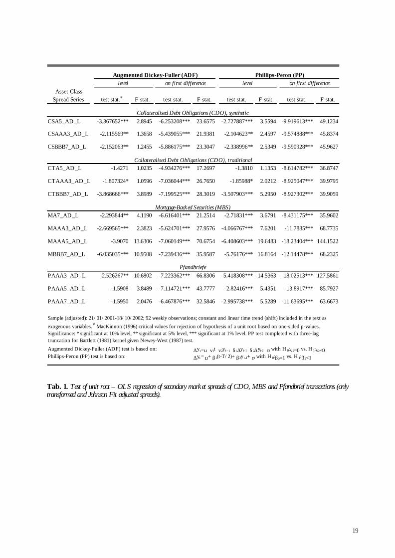
Similar to Koutmos (2002) with respect to U.S. MBS Spreads we reject the unit root in most weekly

spread time series for level data (see Tab. 1). Merely PAAA5 and PAAA7 spreads seem to be non-

stationary (at least for the ADF test statistic), whereas the MAAA5 spreads yield inconclusive results.

Autocorrelation effects can almost be entirely eliminated for a test specification of up to four lags. For the

first difference of spreads both ADF and PP test diagnostics strongly reject the null hypothesis of a unit

root in all cases. Hence, all spread series are integrated of the order zero or at least one. If spreads are

mean-reverting, standard statistical hypothesis testing is applicable.

Generally, we find that LIBOR rates and spreads of European CDO, MBS and Pfandbrief transactions

share a stationary co-integration vector, i.e. they have a long-term relationship, where most spread series

themselves exhibit a I(0) process. We identify two possible causes for the discrepancies of mean-reverting

properties across all spread series for level data: liquidity and data frequency. First, the fact that our results

are less homogenous compared to Koutmos (2002) could be attributable to the poor data quality.20

Whereas Koutmos used time series data of more than 30 years to substantiate his findings on the level

stationary of U.S. MBS spreads, our limited number of observations over a time period of not even two

years does not engross the same degree of measurability of long range cycles of mean-reversion.

20 Higher ADF and PP test statistics of daily Pfandbrief spreads over the originally generated time period from September 1998 to October 2002 (not reported) indicates that better data quality with respect to data frequency and time period of observations, support the rejection of a unit root. Moreover, the spread series of Pfandbrief spreads over a four-year period include spread quotations of summer 2000, when some German Pfandbrief issues – for the first time in recent history – were downgraded amid the massive liquiditiy crises in global financial markets. While almost all German Pfandbrief transactions were AAA-rated and regarded similarly safe an investment as government bonds, a re-assessment of credit risk in Pfandbriefe sent spreads markedly higher during the second half of 2000. Also the shorter series of weekly Pfandbrief spreads used in this analysis might still suffer from lagged effects on spread volatility from January 2001 onwards.

19

Tab. 1. Test of unit root – OLS regression of secondary market spreads of CDO, MBS and Pfandbrief transactions (only transformed and Johnson Fit adjusted spreads).

Asset Class Spread Series test stat.# F-stat. test stat. F-stat. test stat. F-stat. test stat. F-stat.

CSA5_AD_L -3.367652*** 2.8945 -6.253208*** 23.6575 -2.727887*** 3.5594 -9.919613*** 49.1234

CSAAA3_AD_L -2.115569** 1.3658 -5.439055*** 21.9381 -2.104623** 2.4597 -9.574888*** 45.8374

CSBBB7_AD_L -2.152063** 1.2455 -5.886175*** 23.3047 -2.338996** 2.5349 -9.590928*** 45.9627

CTA5_AD_L -1.4271 1.0235 -4.934276*** 17.2697 -1.3810 1.1353 -8.614782*** 36.8747

CTAAA3_AD_L -1.807324* 1.0596 -7.036044*** 26.7650 -1.85988* 2.0212 -8.925047*** 39.9795

CTBBB7_AD_L -3.868666*** 3.8989 -7.199525*** 28.3019 -3.507903*** 5.2950 -8.927302*** 39.9059

MA7_AD_L -2.293844** 4.1190 -6.616401*** 21.2514 -2.71831*** 3.6791 -8.431175*** 35.9602

MAAA3_AD_L -2.669565*** 2.3823 -5.624701*** 27.9576 -4.066767*** 7.6201 -11.7885*** 68.7735

MAAA5_AD_L -3.9070 13.6306 -7.060149*** 70.6754 -6.408603*** 19.6483 -18.23404*** 144.1522

MBBB7_AD_L -6.035035*** 10.9508 -7.239436*** 35.9587 -5.76176*** 16.8164 -12.14478*** 68.2325

PAAA3_AD_L -2.526267** 10.6802 -7.223362*** 66.8306 -5.418308*** 14.5363 -18.02513*** 127.5861

PAAA5_AD_L -1.5908 3.8489 -7.114721*** 43.7777 -2.82416*** 5.4351 -13.8917*** 85.7927

PAAA7_AD_L -1.5950 2.0476 -6.467876*** 32.5846 -2.995738*** 5.5289 -11.63695*** 63.6673

Augmented Dickey-Fuller (ADF) test is based on: ∆yτ=µ+γ1t+γ2y t−1+δ1∆y t-1+δ2∆yt-2 +εt with H 0 :γ2=0 vs. H 1:γ2<0Phillips-Peron (PP) test is based on: ∆yt=µ+ β1(t-T/2)+ β2y t-1+ εt with H 0:β2=1 vs. H 1:β2<1

Mortgage-Backed Securities (MBS)

Pfandbriefe

Sample (adjusted): 21/01/2001-18/10/2002; 92 weekly observations; constant and linear time trend (shift) included in the text as exogenous variables. # MacKinnon (1996) critical values for rejection of hypothesis of a unit root based on one-sided p-values. Significance: * significant at 10% level, ** significant at 5% level, *** significant at 1% level. PP test completed with three-lag truncation for Bartlett (1981) kernel given Newey-West (1987) test.

Augmented Dickey-Fuller (ADF) Phillips-Peron (PP)l eve l on f irs t di f f erence l eve l on f irst di f ference

Collateralised Debt Obligations (CDO), synthetic

Collateralised Debt Obligations (CDO), traditional

20

Moreover, we need to view the level stationarity of spreads with great caution, given the quality of the data

series. MBS and CDO markets on the one side and the Pfandbrief market on the other side differ

significantly in investment liquidity. The “stale” nature of spread movements in the former combined with

a persistent autoregressive effect in spread residuals for up to more than 20 lags for some CDO tranches

(see Tab. 1) could bias the ADF and PP tests into rejecting the unit root. Yet, strong autocorrelation does

not apply for first differences of spreads, so that at least first order integration (as suggested in the later

model measuring spread dynamics on the basis of spread changes) yields satisfactory characteristics of

mean reversion/stationarity.

5 THE MODEL

5.1 Model specification

The following model aims to describe the distribution and volatility of ABS spreads (CDO, MBS) and

Pfandbrief spreads in Europe. Like the equilibrium models of the term structure of interest rates,21 which

are based on the stochastic process followed by a small number of state variables, each state variable tS of

ABS spreads follows a standard geometric Brownian motion (GBM),

( ){ }20 exp 2 ,t tS S t t zµ σ σ= − + (0.12)

where the volatility process ttzσ – which could be also be written in a discrete sense as

0t ttz W W≡ − – contains a Wiener process defined by the normally distributed variable ( )0,z t∆ ∆∼ ,

whose mean change is zero and variance proportional to t. The dynamics of tS , i.e. the instantaneous

value, is identified by the stochastic differential equation

t t tdS S dt dWµ σ= + , (0.13)

of the Ito process ( ) ( ), ,t t t tdS S t dt S t dWµ σ= + (generalised Wiener process), whose trend and volatility

depend on the current spread level tS and time. In the case of the GBM the drift µ and the volatility σ

are proportional to the current value of tS . tW is a standard Brownian motion, with the infinitesimal

increment of a Brownian motion denoted by a standard Wiener process ε=,x t jdz dt and ε j as a

standard normal random variable. This approach assumes that the normalised changes of spreads t tdS S

follow a standard normal distribution (0,1)N .

21 These models are represented by Ito equations as in Hull (1995 and 1993) and others.

21

We measure the spread dynamics of µ σ= +, ,i t i t tdS S dt dW on the basis of a GARCH multi-factor term

structure model as a discrete approximation of spread change, provided that the spread change follows a

stationary process (see section 4). For this purpose we modify the approximative GARCH(1,1) model of

U.S. MBS yields (over government bonds) by Koutmos (2002, 45),22 as we describe the dynamics of

spread change on the basis of additional endogenous factors in a refined GARCH model.

Generally a GARCH(p,q) process models the heteroskedasticity of a given time series Tx , whose

distribution – conditionally on past observations of −t qx – is specified by ( ) ( )σ ∼/ 0,1t tF x of zero

mean and variance of one. The conditional variance of the mean value follows a GARCH process defined

by the volatility from the previous period(s), measured as the q lag(s) of the squared residual(s) from the

mean equation (ARCH term(s)) and the forecast variance(s) of the last p periods (GARCH term(s)).

The adapted original two-factor GARCH(1,1) model by Longstaff and Schwartz (1992) as discrete

approximation of continuous spread change would read

α α α σ ε− −− ≡ ∆ = + + +21 0 1 1 2t t t t t tS S S S (0.14)

σ β β ε β β σ− − −= + + +2 2 20 1 1 2 1 3 1t t t tS , (0.15)

for ( ) ( )σ∆ ∼/ 0,1t tF S .

The equations of the mean and the conditional variance of spreads above capture any past influence on

both spread change ∆ tS (mean equation) and conditional variance σ 2t . If the mean reversion parameter

α <1 0 , the spread series is considered level stationary. The conditional mean of spread change is

dependent on the past spread level −1tS and the level of the conditional variance, with error term ε t . The

conditional variance follows a GARCH(1,1) process, which is defined by one lag squared errors ε −2

1t in

the mean equation, the autocorrelation term (forecast variance of the previous period) σ −2

1t and the past

spread level (as extension to the standard GARCH(1,1) model).

Since both equations do not recognise asymmetric spread dynamics, Koutmos (2002) proposes a two-

factor model, which accommodates mean reversion in U.S. MBS yields after positive and negative past

spread changes in line with Bali (2000). Koutmos breaks down both the mean reversion term α1 (mean

22 Building on the two-factor model by Longstaff and Schwartz (1992) and the work by Bali (2000, 192) on to stochastic volatility models of short-term interest rates, Koutmos considers frequently observed volatility clusters of yield curves (GARCH effect) in the context of asymmetric mean reversion. He finds that spreads commonly behave non-stationary if a positive spread change in the past had preceded an external shock, whilst mean reversion is statistically significant after negative spread change.

22

equation) into ( )α α− −+ −1, 1 1, 11p t t n t tI S I S by imposing the indicator function −

−

− ≥= − <

1

1

1 if 00 if 0

t tt

t t

S SI

S S on

the first moment of one lag spreads. Moreover, he also introduces asymmetry in the conditional variance

equation by discriminating between the coefficient value of positive and negative squared residuals of the

previous period by means of an extended ARCH term ( )β ε β ε− − − −+ =2 21 1 2 1 1 1for min 0,t t t tu u instead of

β ε −2

1 1t (ordinary ARCH term) only. Here, 1β measures any general sensitivity of the conditional variance

σ 2t to past squared residuals, while the coefficient value of β2 is limited to the contribution of negative

past errors ε − <1 0t to the variance and, hence, reflects any degree of potential asymmetries. This

approach differs only formally from the so-called “threshold ARCH” (TARCH) process developed

independently by Glosten et al. (1993) and Zakoian (1990), which allows asymmetric shocks to volatility

through the ARCH term ε

β ε γεε

−− − −

−

≥+ =

<

22 2 1

1 1 1 1 21

0 if 0for

1 if 0t

t t tt

d d . In the original TARCH setting

introduced by Engle and Ng (1993) in their research on the impact of news on volatility (asymmetric

News Impact Curve), good news ε − <1 0t and bad news ε − >1 0t have different effects on the conditional

variance. Good news has an impact of β1 , while bad news has an impact of β γ+1 . If γ ≠ 0 the news

impact is asymmetric, where γ > 0 signifies a “leverage effect”.

5.2 GARCH specification

In this paper we explain the heteroskedasticity spread change behaviour (term structure of spreads) by a

multi-factor asymmetric GARCH process (GARCH(1,1) and GARCH(2,1)) on the basis of two equations

for the mean and conditional variance. In extension to Koutmos’ (2002) adaptation of Longstaff and

Schwartz (1992), the conditional mean is influenced by past spread levels, the past LIBOR rate and the

conditional variance. The latter follows a GARCH process defined by past variance (GARCH term), past

squared residuals of the mean equation (ARCH term) as well as the LIBOR rate and past spreads as

variance regressors. We find the LIBOR rate as an appropriate reference base for the given spread series

(Goodman and Ho, 1998). In contrast to Koutmos, however, our sample size is limited to 93 weekly

observations of actual secondary market spread data for traded tranches of theses asset types. In order to

improve the statistical properties of the analysis we adjusted the spread series and transformed them, so

that the subsequent examination could be completed on “raw” data, logarithmic spreads and spreads

adjusted by the Johnson Fit. The spread series of LIBOR enters the estimation only as observed spot rates

and logarithmic spot rate without Johnson Fit.

In the GARCH(1,1) model we incorporate (i) the first moment of LIBOR changes (with indicator

function) in the mean equation and (ii) the past LIBOR rate as variance regressor. In an alternative

GARCH(2,1) process, we refine the GARCH(1,1) model as we (i) introduce a new set of mean reversion

coefficients of lag two for positive and negative past spread levels mean equation (with a corresponding

23

indicator function) and (ii) extend the past forecast variance to two lags in the estimation of conditional

variance. Overall, we consider asymmetric effects of explanatory factors through (i) indicator functions for

past spreads and past LIBOR rates in the mean equation as well as (ii) two coefficients for positive and

negative errors in the expression for conditional variance.

5.2.1 GARCH(1,1) model specification

We specify the GARCH(1,1) model by the following mean equation and conditional variance equation:

( )

( )α α α

α α α σ ε− − −

− −

− ≡ ∆ = + + − +

+ − + +1 0 1,1 1 1,2 1

22,1 1 2,2 1 3

1

1t t t t t t t

t t t t t t

S S S I S I S

K L K L, (0.16)

which specialises to

( ) ( ) ( ) ( )

( ) ( ) ( )α α α

α α α σ ε− −

− −

∆ = + + − +

+ − + +0 1,1 1 1,2 1

22,1 1 2,2 1 3

ln ln 1 ln

ln 1 lnt t t t t

t t t t t t

S I S I S

K L K L (0.17)

and

σ β β ε β β β β σ− − − − −= + + + + +2 2 2 20 1 1 2 1 3 1 4 1 5 1t t t t t tu S L , (0.18)

which specialises to

( ) ( )σ β β ε β β β β σ− − − − −= + + + + +2 2 2 20 1 1 2 1 3 1 4 1 5 1ln lnt t t t t tu S L , (0.19)

where tS denotes the secondary market spreads of a certain asset class of CDO, MBS or Pfandbrief and

tL is the 3-month-LIBOR rate both at time t.23 The indicator function of past innovations (negative and

positive) is expressed as ( )ε− −=1 1min 0,t tu . The indicator functions for the first difference of spreads tS

and LIBOR rates tL are −

−

− ≥= − <

1

1

1 if 00 if 0

t tt

t t

S SI

S S and −

−

− ≥= − <

1

1

1 if 00 if 0

t tt

t t

L LK

L L respectively.

In the above GARCH(1,1) expression the first order spread change depends on the spread level of the

previous period (conditional on the direction of change), the change of the sport rate (LIBOR) of the

previous period as reference base and the conditional variance with a past volatility forecast (GARCH

term) and lagged squared residuals from the mean equation (ARCH term). The use of one lag spreads

captures first-order autocorrelation. The inclusion of the LIBOR rate as proxy for the general interest rate

level is crucial control factor of our analysis, because a statistically significant effect of LIBOR as the most

prominent fixed income benchmark helps specify the nature of spread changes due to idiosyncratic effects

in the ABS market. The squared residuals measure the part of spread changes that escape the explanatory

23 Note that this specification could be modified to control for first differences in LIBOR changes. An extension of this paper incorporates this consideration.

24

power of independent factors in the mean equation. Hence, they measure mainly those parts of changes in

the spread over time, which are common to the pricing of structured debt.

Moreover, model allows the examination of asymmetric effects of past spread levels and the squared

errors on future spread dynamics. If the regression coefficients α α≠1,1 1,2 and α α+ <1,1 1,2 0 the given

spread series is level stationary with asymmetric mean reversion at lag one. Analogously, the same applies

for the relationship between α α2,1 2,2and in the context of lag two. Moreover, past errors have different

effects on the conditional variance. β1 measures any general sensitivity of the conditional variance to past

errors, whereas β 2 measures the impact of negative past error ε − <1 0t on the conditional variance and,

hence, reflects any degree of potential asymmetries for β ≠2 0 . The contribution of an (overall) positive

error ε − >1 0t will be equal to β β+1 2 . If β >2 0 , the conditional variance of spread change is more

sensitive to positive past errors (i.e. spread increases) than negative past errors (i.e. spread decreases).

However, if β <2 0 negative residuals precede a negative reaction in spread change. β3 and β4 measure

the sensitivity of variance to the spread level and the LIBOR rate, while β5 represents its persistence.

5.2.2 GARCH(2,1) model specification

In extension to the GARCH(1,1) model we allow for a greater explanatory power by past volatility in a

GARCH(2,1) process, as we expand the forecast variance of the conditional variance to the last two

periods, which is matched by two lag spreads as additional independent variable in the mean equation to

control for second-order autocorrelation. Squared errors in the conditional variance expression are kept at

one lag.

( ) ( ) ( ) ( ) ( )

( ) ( ) ( ) ( ) ( )α α α α

α α α α σ ε− − −

− − −

∆ = + + − + +

− + + − + +0 1,1 1 1,2 1 2,1 2

22,2 2 3,1 1 3,2 1 3

ln ln 1 ln ln

1 ln ln 1 lnt t t t t t t

t t t t t t t t

S I S I S J S

J S K L K L, (0.20)

and

( ) ( )σ β β ε β β β β σ β σ− − − − − −= + + + + + +2 2 2 2 20 1 1 2 1 3 1 4 1 5 1 6 2ln lnt t t t t t tu S L , (0.21)

where the indicator function for changes in the two lag spread difference of tS is −

−

− ≥= − <

2

2

1if 00if 0

t tt

t t

S SJ

S S.

The estimation of the presented GARCH models requires a non-linear solution algorithm for conditional

maximum likelihood (CML). We apply two kinds of maximum likelihood iterative estimation procedures –

Berndt-Hall-Hall-Hausman(BHHH)/Gauss-Newton (1974)24 and Marquardt (1963)25. Since the first moment

24 The shared underlying approximative estimation algorithm is referred to as Gauss-Newton for general nonlinear least squares problems, and Berndt, Hall, Hall, and Hausman (BHHH) for maximum likelihood problems. For both types of

25

of logarithmic spreads of most time series in our data set does not follow a normal distribution (see

Appendix, Tab. 9-Tab. 11) with the exception of some Pfandbrief issue spreads, we use the

heteroskedasticity consistent covariance method by Bollerslev and Wooldridge (1992), which is needed for

several model diagnostics (coefficient and residual tests). In this way, we derive robust estimators for

quasi-maximum likelihood (QML) covariance and standard errors (Bollerslev and Woolridge, 1992, 145-

150) even in absence of normally distributed spread differences.

Since both the maximum-neighbourhood procedure of the Marquardt ML algorithm and the

approximation of the negative Hessian by the sum of the gradient vectors of the Berndt, Hall, Hall, and

Hausman (BHHH) algorithm use random iterative components, the estimation for one and the same

spread series could yield different results each time. This holds true especially for short time series, such as

in our case of CDO, MBS and Pfandbrief spreads, where disparate local optima misrepresent the overall

estimation result. In order to derive estimation results at parameter values that maximise the objective

function (global optimum), we devise a specific estimation procedure. After N iterative cycles generates

preliminary estimation results, we perpetuate the estimation process until the adjusted R2-measure and the

significance of estimators squares up with the best results after the first N number of estimations. The

determination of N represents a trade-off between computational time and the consistency of the

successive estimations given the length of the time series. We set = 1,000N for the short time series of

weekly spreads. The estimation procedure is conducted with simple OLS-estimators

× × × × ×1, 0.7, 0.5, 0.3 or 0 of the specified equation as three different starting values, where the starting

value of ×0.7 were used in cases when the estimation algorithm encountered a singular matrix due to

multicollinearity of model factors.26

problems this estimation routine represents the substitution of the negative Hessian by an approximation derived from the summed outer product of the gradient vectors of each observation’s contribution to the objective function. It is asymptotically equivalent to the actual Hessian when evaluated at the parameter values that maximise the objective function. Advantages of Gauss-Newton/BHHH are that only the first derivatives need to be evaluated and the outer product is necessarily positive definite. However, this approximation algorithm performs poorly and may provide a poor guide to the overall shape of the function, when evaluated at parameter values away from the maxium, so that more iterations may be needed for convergence. 25 The Marquardt ML algorithm is based on a maximum-neighbourhood procedure, which combines the benefits of both Gauss algorithms and gradient procedures. According to Marquardt (Marquardt, 1963, 431) pure Gaussian estimation procedures frequently fail due to the divergence of successive iterative steps, whereas gradient procedures only gradually reach the necessary level of convergence if the approximate solution optimum has been determined already. The Marquardt ML estimation procedure does not share these drawbacks. Its algorithm quickly converges to the solution optimum (similar to Gauss algorithms) and pushes the updated parameter values in the direction of the gradient. Like in gradient procedures, the Marquardt estimation aims to find the optimum based on random solution values far removed from the area of convergence of other iterative estimation procedures (Marquardt, 1963, 441). The Marquardt algorithm modifies the Gauss-Newton algorithm in exactly the same manner as quadratic hill climbing modifies the Newton-Raphson method (by adding a correction matrix (or ridge factor) to the Hessian approximation). Note that in the Marquardt estimation we compute asymptotic standard errors from the unmodified (Gauss-Newton) Hessian approximation once convergence is achieved. 26 As an alternative to applying SQR-GARCH estimation in cases, when multicollinearity of estimation yields a singular matrix only for any starting value of simple OLS-estimators, we could also skip the intercept term α0 (i.e. the constant of spread differences) from the estimation equation. This remedial procedural, however, would only be commendable if the statistical significance of the intercept term is neglegible for the interpretion of the estimation results. Particularly in context of the GARCH(2,1) specification, high levels of significance of the intercept prohibit this approach.

26

Upon estimation of the two specifications of GARCH models, we examine the degree of level stationarity

– the influence of past spread levels on future spread change that is – contingent on past positive and

negative spread change (coefficient test). In order to attest overall mean reversion to the given spread

dynamics we validate the hypotheses for the coefficient values α α+ <1,1 1,2 0 in GARCH(1,1) and

α α α α+ < + <1,1 1,2 2,1 2,20and 0 in GARCH(2,1) respectively. Each hypothesis is comprised of two sub-

hypotheses: these are α α+ =0,1 1,1 1,2: 0H and α α α α+ = +0,2 1,1 1,2 1,1 1,2ˆ ˆ:H for both GARCH models as

well as α α+ =0,1 2,1 2,2: 0H and α α α α+ = +0,2 2,1 2,2 2,1 2,2ˆ ˆ:H for GARCH(2,1) in order to account for

past spread levels of up to lag two. The time series is overall stationary, if we cannot reject the second null

hypothesis, i.e. sum of the coefficient values is not significantly different from the sum of the calculated

test estimators, and the sum of the coefficients is smaller than zero, so that the first null hypothesis is

rejected. Furthermore, in context of measuring the heteroskedasticity of spreads we also assess any

asymmetry of spread dynamics. If α α=0 1,1 1,2:H for GARCH(1,1) as well as α α=0 1,1 1,2:H and

α α=0 2,1 2,2:H for GARCH(2,1) can be rejected, past spread change influences the effect the sensitivity

of future spread change to past spread levels.

Both tests are completed on the basis of the Wald coefficient test, which computes the test statistic by

estimating an unrestricted regression without imposing the coefficient restrictions specified by the null

hypothesis. Hence, it tests the validity of linear coefficient restrictions as it measures how close the

unrestricted estimates come to satisfying the restrictions under the null hypothesis. In matrix algebra the

null hypothesis is generally written as β =R0 :H r , where r denotes the × 1m vector of the required

results of the testable restrictions and m is the number of restrictions. The matrix ( )×R m k represents the

linear combinations of the restrictions, with β as the coefficient vector with k number of coefficients. 27

The Wald test diagnostic is calculated from

( ) ( )( ) ( )β σ β χ−−

=′ ′ ′= − × −R R X X R R ∼112 2

df mW r r ,28 (0.22)

where σ 2 is the variance of unrestricted residuals.

27 For instance, the validity of the joint hypotheses of 1 2 1β β+ = and 3 4β β= would require the following

specification of the Wald test for 2m = and 4k = :

ββββ

⊗ = −

1

20

3

4

1 1 0 0 1:

0 0 1 1 0H (Hamilton, 1994, 205f).

28 Under the assumption of independent and normally distributed residuals ε , we calculate the F-statistic

( ) ( )( ) ( )112 1F r s r mβ β

−− −′ ′ ′= − × × − ×R R X X R R , where 1m = is equal to the value of W and 2s poses as

estimator of 2σ (Hamilton, 1994, 206).

27

Finally, we determine the correct specification of both modified GARCH models on the basis of three

residual tests. We check the Llung-Box (LB) Q-statistic for standardised and squared standardised residuals

of the estimation process in order to detect any remaining serial correlation in the mean equation and any

remaining ARCH effect in the conditional variance equation respectively. If the mean equation is correctly

specified, all Q-statistics for standardised residuals should be insignificant with no observable

autocorrelation. Analogously, the same applies to the LB Q-statistic for squared standardised residuals of

correctly specified conditional variance. Moreover, we resort to the Jarque-Bera statistic for standardised

residuals as statistical diagnostic in order to test the null hypothesis of a normal distribution assumption of

errors.

6 ESTIMATION RESULTS

Tab. 2 and Tab. 3 report the Berndt-Hall-Hall-Hausman (BHHH) estimation results for the multi-factor

GARCH(1,1) and GARCH(2,1) models with asymmetric mean reversion on the basis of Johnson-Fit-

adjusted and logarithmic spreads. Generally, the specified factors have relatively weak influence on

conditional spread differences in GARCH(1,1) and conditional variance in GARCH(2,1) of MBS tranches,

while all other spread series of other asset classes confirm the high degrees of explanatory power to

designated model factors.

The intercept coefficient is significant for all spread series in the GARCH(2,1) model with the exception

of all Pfandbrief tranches and MAAA5. In GARCH(1,1) the picture reverses, where the constant is only

significant for CSAAA3, MBBB7 and PAAA7. The influence of past spreads on future spread change – be

it at lag one ( )1,1 1,2,α α in the GARCH(1,1) specification or up to two lags ( )1,1 1,2 2,1 2,2, and ,α α α α in

GARCH(2,1) – clearly supports the degree of mean reversion observed in the unit root test for the given

coefficient values and the level of statistical significance. In all spread series the coefficients for past

spreads levels with subsequent negative and positive spread change sum up to negative values, indicating

level stationarity. Moreover, asymmetric mean reversion is more pronounced for low-rated MBS

transactions and all Pfandbriefe time series, whose spread development and pricing pattern might be

attributable to higher market liquidity and different asset-specific investor sentiment compared to CDO

deals. The time series of all asset classes in the GARCH(1,1) model as well as all but the time series of

traditional CDO transaction exhibit higher effects of negative spread change at lag one ( )1,2α . The

coefficients 1,1 1,2andα α in both GARCH models share similar significance across the given spreads

series, so that first order stationarity follows both negative and positive past spread change. In

GARCH(1,1), however, the mean reversion coefficients are significant only for one out of six CDO

tranche categories, two out of four MBS and all Pfandbrief transactions

28

Considering – where appropriate and statistically significant – the null hypothesis of future spread change

irrespective of whether past spreads increased or declined, we find higher spread sensitivity to past spread

levels associated with negative first moments (negative asymmetric mean reversion). All cases in

GARCH(1,1) show this pattern of asymmetric mean reversion.

The asymmetric effect of past spread change reverses for second differences of past spread levels in the

GARCH(2,1) specification, where the spread reaction after positive shocks is more pronounced. We

detect exactly the opposite effect of two lag spread change in the GARCH(2,1) model, so that the

response to positive spread changes ( )2,1α dominates the negative effects ( )2,2α . This negative pricing

bias might be attributable to the depressed economic outlook and cautious investor behaviour during the

time the sample was taken. However, their statistical significance is the same for each type of spread

series. All three traditional CDO and three out of four MBS spread series do not generate significant

2,1 2,2andα α coefficients. Level effects in 0α seem to be limited to CDOs and MBSs in the GARCH(2,1)

model only, where spread change remain almost unaffected by the LIBOR rate of the previous period

(except for CDOs in the GARCH(2,1) model) as documented by coefficients 2,1 2,2andα α in

GARCH(1,1) and 3,1 3,2andα α in GARCH(2,1) . The coefficients 3α and 4α , which measure the direct

influence of the conditional variance on spread change, are significant for PAAA7 spreads in

GARCH(1,1) and CTAAA3 in GARCH(2,1). Surprisingly, neither the short time series nor the relative

illiquid nature of CDO and MBS spreads in our data set induce pseudo-causalities – a situation that might

reasonably explain why the z-statistics of CSAAA3 and MAAA5 in GARCH(1,1) as well as CSAAA3 and

CSA5 in GARCH(2,1) are shy of reaching the 10% significance threshold by a margin only. No conclusive

assessment can be made as regards the coefficient values of 3α and 4α , whose signs do not seem to be

associated with either a certain rating quality, maturity or asset class of the tranches (spread series).

We do not obtain a homogenous result for the estimator of the constant 0β in either GARCH model.

While most spread series generate positive intercept values, significant estimators are limited to CSA5,

CTA5, MAAA3 and MA7 tranche types in GARCH(1,1) and CSAAA3, CTAAA3, CTA5 and PAAA7 in

GARCH(2,1).

The coefficient 1β measures any general sensitivity of the conditional variance to past residuals (ARCH

effects) of estimated spread change. In all cases but BBB-rated traditional CDO transactions (CTBBB7)

we cannot reject that the conditional variance of spread changes is not dependent on past errors 1β

(ARCH term) as spreads increase, whilst in both GARCH models negative past errors 2β (ARCH term)

for spread decline (negative ARCH effect) are significant in many instances, e.g. Pfandbriefe with short

maturities and high-rated traditional CDOs. Since 1 2β β+ measures the dependence on positive past

errors and 2β measures the influence of negative past errors, 2 0β ≠ reflects potential asymmetries of

29

how past errors generally affect conditional variance. We find 2 0β > in most spread series (with negative

signs only for two out of three traditional CDO tranche types in GARCH(1,1) and two out of four MBS

tranche types in GARCH(2,1)). Moreover, significant 2β are always positive (with the only exception of

the CTA5 spread series in GARCH(1,1)). Since negative effects of past squared residuals dominate the

general effect of residuals by absolute value for both GARCH models, the conditional variance 2tσ of

spread change is more sensitive to negative past errors (i.e. spread declines).29

The predominantly positive influence of 2β negative innovations (i.e. spread declines) on the conditional

variance in both GARCH specifications documents that volatility is asymmetric, i.e. negative past errors

increase spread volatility more than positive innovations (i.e. spread increases) – similar to stock price

volatility. Apparently, the asymmetry of spread dynamics for the given time period captured by the sample

size is not only limited to the mean equation alone but extends to the conditional variance, too. In our

specific case, nearly all spread series exhibit an increase of conditional variance after a spread decrease and

negative past innovations. Since our longer time series of Pfandbrief spreads (from 1998 to 2002) confirm

this results to the extent that past errors (i.e. spread changes) have a positive effect or no effect at all on

the conditional variance, we can rule out that asymmetric spread volatility merely reflects a specific pattern

of spread dynamics with transitory validity.

As we define positive contribution of past errors as 1 2β β+ the degree of the asymmetric effect of past

errors on spread volatility is captured by the metric ( )1 2 1β β β+ (“asymmetry factor” of conditional

variance). Across most ARCH terms in both GARCH models the asymmetry factor is greater than one

(with the exception of negative values for CSAAA3, CSA5 and CTAAA3 in both models, i.e. no

asymmetry in conditional variance, and values between 0 and 1 for MAAA3 in GARCH(1,1) as well as

CTBBB7 and MBBB7 in GARCH(2,1). It also decreases the longer the maturity and the lower the rating

grade of the given spread series. In general, the GARCH(2,1) specification seems to produce a more

consistent degree of asymmetry than the GARCH(1,1) model. Particularly in the former specification, the

asymmetry factor of more than two in most spread series indicates that negative past errors of spread

estimates (negative innovations/spread decline) increase the spread volatility twice as much than positive

past errors (spread increase).

29 See also Bali (2000), 210f.

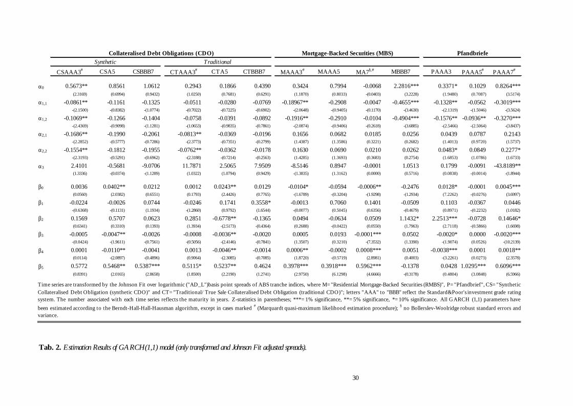
30

Tab. 2. Estimation Results of GARCH(1,1) model (only transformed and Johnson Fit adjusted spreads).

CSAAA3# CSA5 CSBBB7 CTAAA3# CTA5 CTBBB7 MAAA3# MAAA5 MA7§,# MBBB7 PAAA3 PAAA5# PAAA7#

α0 0.5673** 0.8561 1.0612 0.2943 0.1866 0.4390 0.3424 0.7994 -0.0068 2.2816*** 0.3371* 0.1029 0.8264***(2.3169) (0.6994) (0.9432) (1.0250) (0.7681) (0.6291) (1.1870) (0.8033) -(0.0403) (3.2228) (1.9480) (0.7087) (3.5174)

α1,1 -0.0861** -0.1161 -0.1325 -0.0511 -0.0280 -0.0769 -0.18967** -0.2908 -0.0047 -0.4655*** -0.1328** -0.0562 -0.3019***-(2.1500) -(0.8382) -(1.0774) -(0.7022) -(0.7225) -(0.6902) -(2.0648) -(0.9405) -(0.1170) -(3.4630) -(2.1319) -(1.5046) -(3.5624)

α1,2 -0.1069** -0.1266 -0.1404 -0.0758 -0.0391 -0.0892 -0.1916** -0.2910 -0.0104 -0.4904*** -0.1576** -0.0936** -0.3270***-(2.4369) -(0.9098) -(1.1281) -(1.0653) -(0.9835) -(0.7861) -(2.0874) -(0.9406) -(0.2618) -(3.6885) -(2.5466) -(2.5064) -(3.8437)

α2,1 -0.1686** -0.1990 -0.2061 -0.0813** -0.0369 -0.0196 0.1656 0.0682 0.0185 0.0256 0.0439 0.0787 0.2143-(2.2852) -(0.5777) -(0.7286) -(2.3773) -(0.7351) -(0.2799) (1.4387) (1.3586) (0.3221) (0.2682) (1.4013) (0.9720) (1.5737)

α2,2 -0.1554** -0.1812 -0.1955 -0.0762** -0.0362 -0.0178 0.1630 0.0690 0.0210 0.0262 0.0483* 0.0849 0.2277*-(2.3193) -(0.5291) -(0.6962) -(2.3188) -(0.7214) -(0.2563) (1.4285) (1.3693) (0.3683) (0.2754) (1.6853) (1.0786) (1.6733)

α3 2.4101 -0.5681 -9.0706 11.7871 2.5065 7.9509 -8.5146 0.8947 -0.0001 1.0513 0.1799 -0.0091 -43.8189**(1.3336) -(0.0374) -(1.1289) (1.0322) (1.0794) (0.9429) -(1.3835) (1.3162) (0.0000) (0.5716) (0.0838) -(0.0014) -(1.8944)

β0 0.0036 0.0402** 0.0212 0.0012 0.0243** 0.0129 -0.0104* -0.0594 -0.0006** -0.2476 0.0128* -0.0001 0.0045***(0.0560) (2.0382) (0.6551) (0.1793) (2.4426) (0.7765) -(1.6789) -(0.3204) -(1.9298) -(1.2934) (7.2262) -(0.0276) (3.6997)

β1 -0.0224 -0.0026 0.0744 -0.0246 0.1741 0.3558* -0.0013 0.7060 0.1401 -0.0509 0.1103 -0.0367 0.0446-(0.6368) -(0.1131) (1.1934) -(1.2860) (0.9792) (1.6544) -(0.0077) (0.5045) (0.6356) -(0.4679) (0.8971) -(0.2232) (1.0182)

β2 0.1569 0.5707 0.0623 0.2851 -0.6778** -0.1365 0.0494 -0.0634 0.0509 1.1432* 2.2513*** -0.0728 0.14646*(0.6341) (0.3310) (0.1393) (1.3934) -(2.5173) -(0.4364) (0.2688) -(0.0422) (0.0550) (1.7963) (2.7118) -(0.5866) (1.6698)

β3 -0.0005 -0.0047** -0.0026 -0.0008 -0.0036** -0.0020 0.0005 0.0193 -0.0001*** 0.0502 -0.0020* 0.0000 -0.0020***-(0.0424) -(1.9611) -(0.7561) -(0.5056) -(2.4146) -(0.7841) (1.3507) (0.3210) -(7.3532) (1.3390) -(1.9074) (0.0526) -(10.2139)

β4 0.0001 -0.0110** -0.0041 0.0013 -0.0046** -0.0014 0.0006** -0.0002 0.0008*** 0.0051 -0.0038*** 0.0001 0.0018**(0.0114) -(2.0897) -(0.4896) (0.9064) -(2.3085) -(0.7085) (1.8720) -(0.5719) (2.8981) (0.4003) -(3.2261) (0.0273) (2.3578)

β5 0.5772 0.5468** 0.5387*** 0.5115* 0.5237** 0.4624 0.3978*** 0.3918*** 0.5962*** -0.1378 0.0428 1.0295*** 0.6096***(0.8391) (2.0165) (2.8658) (1.8500) (2.2190) (1.2741) (2.9750) (6.1298) (4.6666) -(0.3178) (0.4804) (3.0848) (6.5966)

Time series are transformed by the Johnson Fit over logarithmic ("AD_L")basis point spreads of ABS tranche indices, where M="Residential Mortgage-Backed Securities (RMBS)", P="Pfandbrief", CS="SyntheticCollateralised Debt Obligation (synthetic CDO)" and CT="Traditional/True Sale Collateralised Debt Obligation (traditional CDO)"; letters "AAA" to "BBB" reflect the Standard&Poor's investment grade ratingsystem. The number associated with each time series reflects the maturity in years. Z-statistics in parentheses; ***=1% significance, **=5% significance, *=10% significance. All GARCH (1,1) parameters havebeen estimated according to the Berndt-Hall-Hall-Hausman algorithm, except in cases marked # (Marquardt quasi-maximum likelihood estimation procedure); § no Bollerslev-Woolridge robust standard errors andvariance.

Collateralised Debt Obligations (CDO)Synthetic Traditional

Mortgage-Backed Securities (MBS) Pfandbriefe

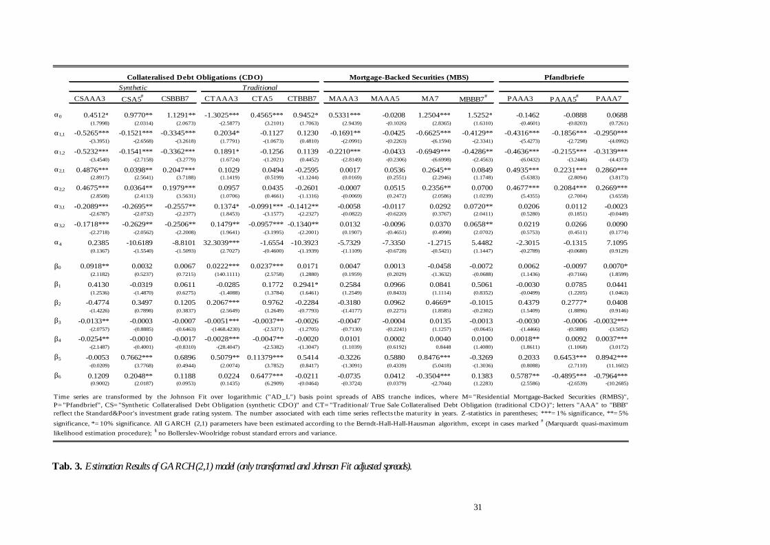
31

Tab. 3. Estimation Results of GARCH(2,1) model (only transformed and Johnson Fit adjusted spreads).

CSAAA3 CSA5# CSBBB7 CTAAA3 CTA5 CTBBB7 MAAA3 MAAA5 MA7 MBBB7# PAAA3 PAAA5# PAAA7

α0 0.4512* 0.9770** 1.1291** -1.3025*** 0.4565*** 0.9452* 0.5331*** -0.0208 1.2504*** 1.5252* -0.1462 -0.0888 0.0688(1.7998) (2.0314) (2.0673) -(2.5877) (3.2101) (1.7063) (2.9439) -(0.1026) (2.8365) (1.6310) -(0.4601) -(0.8203) (0.7261)

α1,1 -0.5265*** -0.1521*** -0.3345*** 0.2034* -0.1127 0.1230 -0.1691** -0.0425 -0.6625*** -0.4129** -0.4316*** -0.1856*** -0.2950***-(3.3951) -(2.6568) -(3.2618) (1.7791) -(1.0673) (0.4810) -(2.0991) -(0.2263) -(6.1594) -(2.3341) -(5.4273) -(2.7298) -(4.0992)

α1,2 -0.5232*** -0.1541*** -0.3362*** 0.1891* -0.1256 0.1139 -0.2210*** -0.0433 -0.6949*** -0.4286** -0.4636*** -0.2155*** -0.3139***-(3.4540) -(2.7158) -(3.2779) (1.6724) -(1.2021) (0.4452) -(2.8149) -(0.2306) -(6.6998) -(2.4563) -(6.0432) -(3.2446) -(4.4373)

α2,1 0.4876*** 0.0398** 0.2047*** 0.1029 0.0494 -0.2595 0.0017 0.0536 0.2645** 0.0849 0.4935*** 0.2231*** 0.2860***(2.8917) (2.5641) (3.7188) (1.1419) (0.5199) -(1.1244) (0.0169) (0.2551) (2.2946) (1.1748) (5.6383) (2.8094) (3.8173)

α2,2 0.4675*** 0.0364** 0.1979*** 0.0957 0.0435 -0.2601 -0.0007 0.0515 0.2356** 0.0700 0.4677*** 0.2084*** 0.2669***(2.8508) (2.4113) (3.5631) (1.0706) (0.4661) -(1.1316) -(0.0069) (0.2472) (2.0586) (1.0239) (5.4355) (2.7004) (3.6558)

α3,1 -0.2089*** -0.2695** -0.2557** 0.1374* -0.0991*** -0.1412** -0.0058 -0.0117 0.0292 0.0720** 0.0206 0.0112 -0.0023-(2.6787) -(2.0732) -(2.2377) (1.8453) -(3.1577) -(2.2327) -(0.0822) -(0.6220) (0.3767) (2.0411) (0.5280) (0.1851) -(0.0449)

α3,2 -0.1718*** -0.2629** -0.2506** 0.1479** -0.0957*** -0.1340** 0.0132 -0.0096 0.0370 0.0658** 0.0219 0.0266 0.0090-(2.2718) -(2.0562) -(2.2008) (1.9641) -(3.1995) -(2.2001) (0.1907) -(0.4651) (0.4998) (2.0702) (0.5753) (0.4511) (0.1774)

α4 0.2385 -10.6189 -8.8101 32.3039*** -1.6554 -10.3923 -5.7329 -7.3350 -1.2715 5.4482 -2.3015 -0.1315 7.1095(0.1367) -(1.5540) -(1.5093) (2.7027) -(0.4600) -(1.1939) -(1.1109) -(0.6728) -(0.5421) (1.1447) -(0.2789) -(0.0680) (0.9129)

β0 0.0918** 0.0032 0.0067 0.0222*** 0.0237*** 0.0171 0.0047 0.0013 -0.0458 -0.0072 0.0062 -0.0097 0.0070*(2.1182) (0.5237) (0.7215) (140.1111) (2.5758) (1.2880) (0.1959) (0.2029) -(1.3632) -(0.0688) (1.1436) -(0.7166) (1.8599)

β1 0.4130 -0.0319 0.0611 -0.0285 0.1772 0.2941* 0.2584 0.0966 0.0841 0.5061 -0.0030 0.0785 0.0441(1.2536) -(1.4870) (0.6275) -(1.4088) (1.3784) (1.6461) (1.2549) (0.8433) (1.1114) (0.8352) -(0.0499) (1.2205) (1.0463)

β2 -0.4774 0.3497 0.1205 0.2067*** 0.9762 -0.2284 -0.3180 0.0962 0.4669* -0.1015 0.4379 0.2777* 0.0408-(1.4226) (0.7898) (0.3837) (2.5649) (1.2649) -(0.7793) -(1.4177) (0.2275) (1.8585) -(0.2302) (1.5409) (1.8896) (0.9146)

β3 -0.0133** -0.0003 -0.0007 -0.0051*** -0.0037** -0.0026 -0.0047 -0.0004 0.0135 -0.0013 -0.0030 -0.0006 -0.0032***-(2.0757) -(0.8885) -(0.6463) -(1468.4230) -(2.5371) -(1.2705) -(0.7130) -(0.2241) (1.1257) -(0.0645) -(1.4466) -(0.5880) -(3.5052)

β4 -0.0254** -0.0010 -0.0017 -0.0028*** -0.0047** -0.0020 0.0101 0.0002 0.0040 0.0100 0.0018** 0.0092 0.0037***-(2.1487) -(0.4001) -(0.8310) -(28.4047) -(2.5382) -(1.3047) (1.1039) (0.6192) 0.8448 (1.4080) (1.8611) (1.1068) (3.0172)

β5 -0.0053 0.7662*** 0.6896 0.5079** 0.11379*** 0.5414 -0.3226 0.5880 0.8476*** -0.3269 0.2033 0.6453*** 0.8942***-(0.0209) (3.7768) (0.4944) (2.0074) (3.7852) (0.8417) -(1.3091) (0.4339) (5.0418) -(1.3036) (0.8088) (2.7110) (11.1602)

β6 0.1209 0.2048** 0.1188 0.0224 0.6477*** -0.0211 -0.0735 0.0412 -0.3504*** 0.1383 0.5787** -0.4895*** -0.7964***(0.9002) (2.0187) (0.0953) (0.1435) (6.2909) -(0.0464) -(0.3724) (0.0379) -(2.7044) (1.2283) (2.5586) -(2.6539) -(10.2685)

Time series are transformed by the Johnson Fit over logarithmic ("AD_L") basis point spreads of ABS tranche indices, where M="Residential Mortgage-Backed Securities (RMBS)",P="Pfandbrief", CS="Synthetic Collateralised Debt Obligation (synthetic CDO)" and CT="Traditional/True Sale Collateralised Debt Obligation (traditional CDO)"; letters "AAA" to "BBB"reflect the Standard&Poor's investment grade rating system. The number associated with each time series reflects the maturity in years. Z-statistics in parentheses; ***=1% significance, **=5%

significance, *=10% significance. All GARCH (2,1) parameters have been estimated according to the Berndt-Hall-Hall-Hausman algorithm, except in cases marked # (Marquardt quasi-maximumlikelihood estimation procedure); § no Bollerslev-Woolridge robust standard errors and variance.

Collateralised Debt Obligations (CDO)Synthetic Traditional

Mortgage-Backed Securities (MBS) Pfandbriefe

32

The coefficient β3 measures the sensitivity of the conditional variance to the spread level of the previous

period (“level effect”). We find no coherent results for a significant level effect. β3 carries a negative sign

for the majority of spread series in GARCH(1,1) and all spread series in GARCH(2,1) with the exception

of MA7. The level effect is most significant for Pfandbrief transactions in GARCH(1,1) and traditional

CDOs in GARCH(2,1), where β3 is negative as well. The coefficient β4 measures the level effect of the

underlying reference spot rate (LIBOR rate) of the previous period on conditional variance of spreads.

Past LIBOR rates seem to play some role only for traditional CDOs and Pfandbriefe in both GARCH

models, whereas evidence of possible influence on synthetic CDO structures and MBS is inconclusive.

Finally, we estimate the coefficients 5β for both GARCH specifications and 6β for GARCH(2,1) only in

order to control the estimation of the conditional variance for possible GARCH effects at lag one (and lag

two for GARCH(2,1)). Past variance levels at lag one ( )σ −2

1t are almost always positive (with the

exception of the spread series for MBBB7) and highly significant for almost all time series in the

GARCH(1,1) set-up. In GARCH(1,1) the coefficient values of β5 are positive in most cases of spread

series (with CSAAA3, MAAA3 and MBBB7 carrying negative signs) and are significant especially for

traditional CDO and Pfandbrief transactions. The coefficient β6 documents that most of the explanatory

power of the GARCH term carries over even into the second lag variance forecast in GARCH(2,1). Our

estimation fails to reject the null hypothesis that β6 has no effect on the conditional variance in all

Pfandbrief spreads and in one of each spread series of CDO (traditional and synthetic) and MBS tranche

types at a significance level of at least 5%. In contrast to σ −2

1t evidence of how past forecast variance σ −2

2t

at lag two influences the conditional variance is mixed. Most Pfandbrief spreads and two out of four MBS

spread series exhibit negative GARCH effects for β6 , whereas positive GARCH effects dominate for

CDO transactions in GARCH(2,1). Hence, both β5 and β6 point to the fact that the direction and the

significance of any GARCH effect might depend on the liquidity of the transaction type (with Pfandbrief

transactions being the most liquid and CDO tranches the most illiquid) and, to some extent, data

frequency – the degree of significance and coefficient values of β5 and β6 increase for an extended series

of Pfandbrief spreads (results are not reported in this paper; see also section 3).

Generally, the ARCH and GARCH effects of the conditional variance seem to have greatest statistical

significance for Pfandbriefe and high-rated traditional CDO transactions, while the mean equation with

asymmetric effects of past spread and LIBOR levels generates the closest estimation for the time series of

synthetic CDOs and Pfandbriefe.

We further need to determine the statistical classification of the spread dynamics. We examine the

specification of level stationarity as well as the statistical validity of asymmetric mean reversion based on

the coefficients α α1,1 1,2, (ARCH terms) in the mean equation of GARCH(1,1) and α α1,1 1,2, and α α2,1 2 ,2,

33

in the mean equation of the GARCH(2,1) model. To this end we resort to the Wald coefficient to test the

null hypothesis α α+ <0 1,1 1,2H : 0 ( α α+ <0 2,1 2,2H : 0 for GARCH(2,1) only) for overall mean reversion

of the GARCH models. If α α+ =1,1 1,2 0 the trend has a unit root (random walk) and if α α+ >1,1 1,2 0 the

spread development is explosive, which does not make economic sense. So spread change is level

stationary if we can reject H0. We apply the Wald coefficient test to validate the assumption of

α α+ <1,1 1,2 0 on the basis of two separate sub-hypotheses α α+ =0,1 1,1 1,2: 0H and

α α α α+ = +0,2 1,1 1,2 1,1 1,2ˆ ˆ:H for both GARCH models as well as α α+ =0,1 2,1 2,2: 0H and

α α α α+ = +0,2 2,1 2,2 2,1 2,2ˆ ˆ:H for GARCH(2,1). As shown in Tab. 2 for GARCH(1,1) only one out of six

CDO spread series (CSA5), two out of four MBS spread series (MAAA3 and MBBB7) and two out of

three Pfandbrief spread series (PAAA3 and PAAA5) produce Wald statistics of at least 5% significance, so

that the sum of coefficients α α1,1 1,2, equals the sum of their estimators and differs from zero in all

estimations. Moreover, the trend of each spread series can be determined based on the sign of α α+1,1 1,2ˆ ˆ .

All spread series clearly exhibit negative mean reversion coefficients at lag one.

Tab. 5 reports the results of the Wald-testing procedure for the GARCH(2,1) model coefficients α α1,1 1,2,

and α α2,1 2 ,2, . Here, almost all spread series (with the exception of CSBBB7, CTA3 and MA7) – more

than in the GARCH(1,1) specification – reject the null hypothesis α α+ =0,1 1,1 1,2: 0H at high levels of

significance. Moreover, the sum of coefficients equals the sum of estimators

( )α α α α+ = +0,2 1,1 1,2 1,1 1,2ˆ ˆ:H at a 99% confidence level, and the sum of estimators α α+1,1 1,2ˆ ˆ is negative

for all spread series. Hence, the Wald test for mean reversion for both GARCH models at lag one

confirms our results obtained from the unit root test, which generates the most robust results for

Pfandbrief and MBS spreads. At the same time the degree of mean reversion weakens for the coefficients

α α2,1 2 ,2, at lag two in GARCH(2,1). In comparison to the coefficient values α α1,1 1,2, , all traditional CDO

spread series as well as two out of three Pfandbrief spread series lose their significance of mean reversion

at lag two, so that α α+ =0,1 2,1 2,2: 0H can no longer be rejected. Moreover, the sum of estimators

α α+2,1 2,2ˆ ˆ is positive for all spread series. Hence, in GARCH(2,1) the Wald coefficient test indicates that

CDO transactions fail to unequivocally support mean reversion at lag one and non-stationarity at lag two

for first and second spread differences, whilst MBS spread series show significant level stationarity in

α α+ <1,1 1,2 0 but not for α α+ <2,1 2,2 0 .

We also assess the degree of asymmetry of spread dynamics in context of measuring the heteroskedasticity

of spreads. We test the null hypothesis of no asymmetry for the first spread differences α α=0 1,1 1,2H :

for both GARCH model ( α α=0 2,1 2,2H : for GARCH(2,1) only). The results of both test are reported in

Tab. 4 and Tab. 5.

34

In both GARCH models the null hypothesis of no asymmetry, i.e. future spreads are equally sensitive to

positive or negative first differences of past spreads (spread declines/spread increases), can be rejected at

high confidence intervals for nearly all asset classes for the coefficients α α1,1 1,2, . Merely two MBS spread

series (MAAA3 and MAAA5) and one Pfandbrief type (PAAA7) in GARCH(1,1), and one CDO spread

series (CSBBB7) and one MBS tranche type (MA7) in GARCH(2,1) generate probability values for the H0

as coefficient restriction, which makes the Wald test statistics not significant.30 The significance of

asymmetric effects of previous spread change also persist in the second difference of past spreads of

GARCH(2,1) in Tab. 5 – though at an admittedly lower degree of significance especially for traditional

CDO transactions.

Our estimation results for the mean equation are in general agreement with the findings by Koutmos

(2002) on U.S. MBS spreads. However, in contrast to Koutmos (2002), we find that all spread time series

at one lag (with the exception of traditional AAA-rated CDOs in GARCH(2,1)) generate negative

α α1,1 1,2and coefficients of different explanatory power (with greater effects of negative past spread

change compared to positive changes). Hence, future spreads show varying sensitivity to the direction of

past spread change, while spreads exhibit mean reversion in each case. Consequently, overall mean

reversion for both α α1,1 1,2and is maintained. Interestingly, each time series exhibits the same direction of

asymmetric spread response to both positive and negative past spread differences in both GARCH

models. This observation also holds true for second differences in GARCH(2,1). However, whilst the

absolute coefficient values for negative past spread change ( )α1,2 are consistently higher than for negative

past spread change ( )α1,1 in both GARCH models as in Koutmos (2002), asymmetric mean reversion of

spread change at two lags indicates positive bias if α2,1 and α2,2 are compared in GARCH(2,1), where we

also observe a complete sign reversal as α α2,1 2,2and coefficients carry positive signs in all cases.

Considering the high speed of mean reversion, this result seems plausible. The estimation results for

asymmetric mean reversion of Pfandbrief spreads are contradictory given strong evidence of mean

reversion in the estimation of the GARCH model, while the ADF test (see Tab. 1) indicates the existence

of a unit root in level data, so co-integration is limited to the order of one (I(1) process). The estimation

results in both GARCH models also affirm the high significance of the previous period’s variance forecast

(GARCH term) for the conditional variance ( )β5 . The extended approach of GARCH(2,1) hints to an

even stronger historical effect of past volatility, where two lag past variance ( )β6 exerts a durable

influence on future spread change. Judging by the estimation results for Pfandbriefe, market liquidity

apparently facilitates this effect.

30 The p-value indicates the probability of the tested restriction to be significant for the estimation. In this case, the

2χ -distributed Wald-statistic would not deviate from zero at a commonly accepted level of significance.

35

By and large we corroborate the estimation results of conditional variance in Koutmos (2002). Although

we find that negative past errors ( )β2 increase volatility of spread series more than positive past errors

( )β1 , in contrast to Koutmos (2002) asymmetric squared residuals (ARCH term) from the mean equation

are only significant for negative past errors ( )β2 in several MBS, traditional CDO and Pfandbrief spread

time series. The statistical irrelevance of past positive errors (as spreads increase) is striking and leads to

reservations regarding preliminary statistical interpretation asset classes with particularly low t-statistics of

coefficient estimates, such as MBS in both GARCH models. The model specification in the following

section will address this issue in detail.

If we take into account all estimation results only coefficient values β1 and β2 for Pfandbriefe in

GARCH(1,1) and all CDOs in GARCH(2,1) deliver clear support for asymmetric effect of past errors.

Also for MBS transactions in both GARCH models and Pfandbriefe under the GARCH(2,1) process the

effect of negative past errors (in cases of spread decline) is more prevalent than any positive past errors.

Nonetheless, merely traditional CDO transactions and Pfandbriefe in the GARCH(2,1) model display

high but not sufficiently significant t-statistics for β1 . Moreover, we find that spread levels and LIBOR

rates of the previous period play a modest role in explaining conditional variance as variance regressors,

whose coefficients β3 and β4 show evidence of significance mostly for CDO and Pfandbrief time series.

Only in the GARCH(1,1) model do our estimation results for MBS transactions (7-year maturity) tally

with the findings by Koutmos (2002).

7 MODEL SPECIFICATION

The correct (model) specification of the mean and conditional variance of spread dynamics by means of

standardised residuals – volatility no explained by the model – is vital to the pricing of structured finance

transactions and the management of spread risk. Hence, we apply model diagnostics to both GARCH

specifications in order (i) to detect any remaining non-linear structure/autocorrelation (Llung-Box (LB)

Q-statistic) of estimated standardised errors ( )t tE ε σ and squared standardised errors ( )2t tE ε σ , and

(ii) to test the normality (Jarque-Bera statistic) of standardised residuals (with first and second moments

equal to zero and unity respectively).

Highly significant LB Q-statistics in Tab. 4 and Tab. 5 testify to an almost complete absence of higher

order serial correlation even at lag one in both standardised residuals of the mean equation (i.e.

specification of mean equation) and squared standardised residuals of conditional variance (i.e.

specification of conditional variance equation). Only some MBS spread time series in both GARCH

model specifications retain statistically significant serial correlation in squared standardised residuals up to

36

six lags. Since the LB Q-statistics for standardised residuals indicate no significant autocorrelation, the

inclusion of one lag spread levels in the in the mean equation of the GARCH(1,1) model and up to two

lag spreads in the mean equation of GARCH(2,1) model prove sufficient for the correct specification of

the mean equation, so that no further inclusion of appropriate lagged endogenous variables in the

equation at the cost of losing degrees of freedom is warranted. Also in the specification of conditional

variance we can rule out ARCH effects (significant Q-statistic) in squared standardised residuals for all

asset types but high-rated MBS transactions. With regard to the Jarque-Bera statistic, we find that the null

hypothesis of normally distributed standardised residuals is rejected for all time series with estimation

results (see Tab. 4 and Tab. 5).

Although the Llung-Box (LB) and Jarque-Bera (JB) statistics are commonly accepted and well established

model diagnostics to examine the degree of autocorrelation and normality of standardised residuals,31 they

fail to test how well the proposed GARCH models capture the asymmetric effects on spread volatility, i.e.

the contribution of positive and negative past estimation errors/innovations to changes in conditional

variance (Koutmos, 2002). Since the GARCH processes explain the heteroskedasticity of observed spread

behaviour, the correct specification of the conditional variance equation and any patterns of asymmetric

change is imperative.

In the spirit of the diagnostics developed by Engle and Ng (1993) to test asymmetric effects in the news

impact curve implied by the model estimates of conditional variance, we examine the correct specification

of the asymmetric volatility process of spread dynamics by means of three testing procedures: the

(negative) sign bias test, the negative size bias test and the positive sign bias test. All test rest on the

assumption that the conditional variance is correctly specified only if the squared standardised residuals

escape any predictability through observed variables, which distinguish between positive and negative past

errors (null hypothesis). Hence, if the t-statistics for all three tests are statistically insignificant, the

estimated volatilities from the GARCH models fully incorporate past information (at one lag).

The (negative) sign bias test ( )2t t tK eε σ µ γ= + + measures any statistically significant influence of past

errors 1tε − (at one lag) on squared standardised residuals ( )2t tε σ , which is the volatility not predicted by

conditional variance of the model estimation. Since we define the dummy variable 1K = for 1 0tε − < else

0K = in order to account for asymmetric influences of past errors, a significant t-statistic of K signifies

that the impact of positive and negative past errors on spread volatility is not fully specified in the

asymmetric ARCH terms of the conditional variance equation; unexplained spread volatility still contains

some positive/negative effect by past errors.

31 The Llung-Box Q-statistic of standardised residuals is deemed sufficient for the correct specification of the mean equation at this point, as it merely confirms the estimation results obtained from the OLS regression and the Wald coefficient statistics. However, the correct specification of conditional variance requires a further refinement of autocorrelation tests.

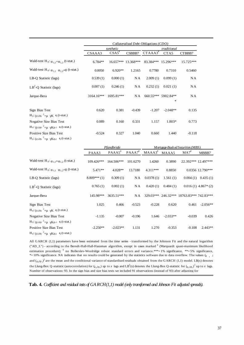
37

Tab. 4. Coefficient and residual tests of GARCH(1,1) model (only transformed and Johnson Fit adjusted spreads).

CSAAA3 CSA5# CSBBB7 CTAAA3# CTA5 CTBBB7

Wald-test H 0: α1,1=α1,2 (t-stat.) 6.784** 16.657*** 13.368*** 83.384*** 15.296*** 15.725***

Wald-test H 0: α1,1+α1,2=0 (t-stat.) 0.0050 6.920** 1.2165 0.7780 0.7310 0.5460

LB-Q Statistic (lags) 0.539 (1) 0.000 (1) NA 2.009 (1) 0.099 (1) NA

LB2-Q Statistic (lags) 0.007 (1) 0.246 (1) NA 0.232 (1) 0.021 (1) NA

Jarque-Bera 3164.16*** 1695.81*** NA 660.55*** 5902.84***

NA

Sign Bias Test 0.620 0.381 -0.439 -1.207 -2.048** 0.135H0: (εt/σt)2=µ+γΚ+et (t-stat.)

Negative Size Bias Test 0.089 0.160 0.331 1.157 1.803* 0.773H0: (εt/σt)2=µ+γΚεt-1+et (t-stat.)

Positive Size Bias Test -0.524 0.327 1.040 0.660 1.440 -0.118H0: (εt/σt)2=µ+γΚεt-1 +et (t-stat.)

PAAA3 PAAA5# PAAA7# MAAA3# MAAA5 MA7# MBBB7

Wald-test H 0: α1,1=α1,2 (t-stat.) 109.426*** 164.506*** 101.6270 1.4260 0.3890 22.392*** 12.497***

Wald-test H 0: α1,1+α1,2=0 (t-stat.) 5.471** 4.028** 13.7180 4.311*** 0.8850 0.0356 12.790***

LB-Q Statistic (lags) 8.809*** (1) 0.309 (1) NA 0.0378 (1) 1.561 (1) 0.004 (1) 0.435 (1)

LB2-Q Statistic (lags) 0.765 (1) 0.002 (1) NA 0.420 (1) 0.484 (1) 0.016 (1) 4.867* (2)

Jarque-Bera 145.98*** 3635.51*** NA 329.03*** 246.32*** 18763.83*** 742.83***

Sign Bias Test 1.025 0.466 -0.523 -0.228 0.620 0.461 -2.056**H0: (εt/σt)2=µ+γΚ+et (t-stat.)

Negative Size Bias Test -1.135 -0.007 -0.196 1.646 -2.033** -0.039 0.426H0: (εt/σt)2=µ+γΚεt-1+et (t-stat.)

Positive Size Bias Test -2.250** -2.023** 1.131 1.270 -0.353 -0.108 2.443**H0: (εt/σt)2=µ+γΚεt-1 +et (t-stat.)

All GARCH (1,1) parameters have been estimated from the time series - transformed by the Johnson Fit and the natural logarithm("AD_L") - according to the Berndt-Hall-Hall-Hausman algorithm, except in cases marked # (Marquardt quasi-maximum likelihoodestimation procedure); § no Bollerslev-Woolridge robust standard errors and variance.***=1% significance, **=5% significance,*=10% significance. NA indicates that no results could be generated by the statistics software due to data overflow. The values (ε τ /σ

and (ετ/στ)2 are the mean and the conditional variance of standardised residuals obtained from the GARCH (1,1) model. LB(x) denotes

the Llung-Box Q-statistic (autocorrelation) for (ετ/στ) up to x lags and LB2(x) denotes the Llung-Box Q-statistic for (ετ/στ)2 up to x lags.

Number of observations: 93. In the sign bias and size bias tests we included 91 observations (instead of 93) after adjusting for

synthetic traditional

Pfandbriefe Mortgage-Backed Securities (MBS)

Collateralised Debt Obligations (CDO)

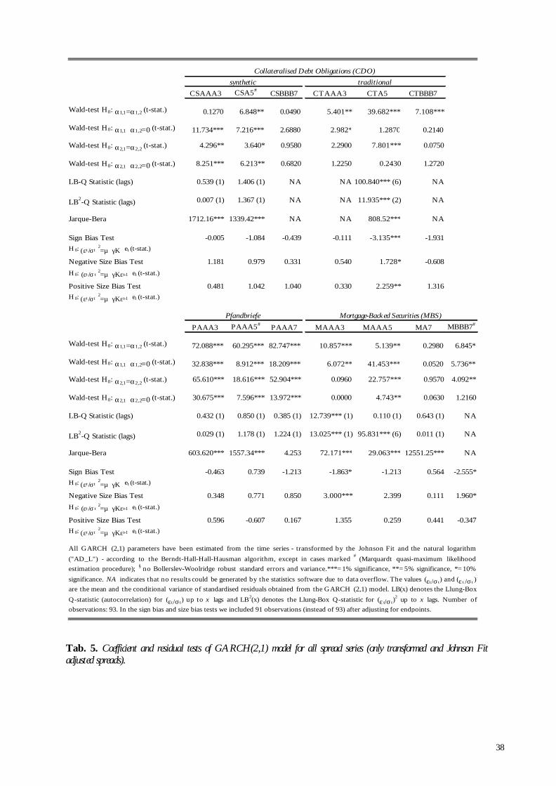
38

Tab. 5. Coefficient and residual tests of GARCH(2,1) model for all spread series (only transformed and Johnson Fit adjusted spreads).

CSAAA3 CSA5# CSBBB7 CTAAA3 CTA5 CTBBB7

Wald-test H0: α1,1=α1,2 (t-stat.) 0.1270 6.848** 0.0490 5.401** 39.682*** 7.108***

Wald-test H0: α1,1+α1,2=0 (t-stat.) 11.734*** 7.216*** 2.6880 2.982* 1.2870 0.2140

Wald-test H0: α2,1=α2,2 (t-stat.) 4.296** 3.640* 0.9580 2.2900 7.801*** 0.0750

Wald-test H0: α2,1+α2,2=0 (t-stat.) 8.251*** 6.213** 0.6820 1.2250 0.2430 1.2720

LB-Q Statistic (lags) 0.539 (1) 1.406 (1) NA NA 100.840*** (6) NA

LB2-Q Statistic (lags) 0.007 (1) 1.367 (1) NA NA 11.935*** (2) NA

Jarque-Bera 1712.16*** 1339.42*** NA NA 808.52*** NA

Sign Bias Test -0.005 -1.084 -0.439 -0.111 -3.135*** -1.931H 0: (εt /σt )

2=µ+γΚ+et (t-stat.)

Negative Size Bias Test 1.181 0.979 0.331 0.540 1.728* -0.608H 0: (εt /σ t)

2=µ+γΚεt-1 +et (t-stat.)

Positive Size Bias Test 0.481 1.042 1.040 0.330 2.259** 1.316H 0: (εt /σt )

2=µ+γΚεt-1+et (t-stat.)

PAAA3 PAAA5# PAAA7 MAAA3 MAAA5 MA7 MBBB7#

Wald-test H0: α1,1=α1,2 (t-stat.) 72.088*** 60.295*** 82.747*** 10.857*** 5.139** 0.2980 6.845*

Wald-test H0: α1,1+α1,2=0 (t-stat.) 32.838*** 8.912*** 18.209*** 6.072** 41.453*** 0.0520 5.736**

Wald-test H0: α2,1=α2,2 (t-stat.) 65.610*** 18.616*** 52.904*** 0.0960 22.757*** 0.9570 4.092**

Wald-test H0: α2,1+α2,2=0 (t-stat.) 30.675*** 7.596*** 13.972*** 0.0000 4.743** 0.0630 1.2160

LB-Q Statistic (lags) 0.432 (1) 0.850 (1) 0.385 (1) 12.739*** (1) 0.110 (1) 0.643 (1) NA

LB2-Q Statistic (lags) 0.029 (1) 1.178 (1) 1.224 (1) 13.025*** (1) 95.831*** (6) 0.011 (1) NA

Jarque-Bera 603.620*** 1557.34*** 4.253 72.171*** 29.063*** 12551.25*** NA

Sign Bias Test -0.463 0.739 -1.213 -1.863* -1.213 0.564 -2.555*H 0: (εt /σt )

2=µ+γΚ+et (t-stat.)

Negative Size Bias Test 0.348 0.771 0.850 3.000*** 2.399 0.111 1.960*H 0: (εt /σ t)

2=µ+γΚεt-1 +et (t-stat.)

Positive Size Bias Test 0.596 -0.607 0.167 1.355 0.259 0.441 -0.347H 0: (εt /σt )

2=µ+γΚεt-1+et (t-stat.)

All GARCH (2,1) parameters have been estimated from the time series - transformed by the Johnson Fit and the natural logarithm("AD_L") - according to the Berndt-Hall-Hall-Hausman algorithm, except in cases marked # (Marquardt quasi-maximum likelihoodestimation procedure); § no Bollerslev-Woolridge robust standard errors and variance.***=1% significance, **=5% significance, *=10%significance. NA indicates that no results could be generated by the statistics software due to data overflow. The values (ετ/στ) and (ετ /στ ) 2

are the mean and the conditional variance of standardised residuals obtained from the GARCH (2,1) model. LB(x) denotes the Llung-BoxQ-statistic (autocorrelation) for (ετ/στ) up to x lags and LB 2(x) denotes the Llung-Box Q-statistic for (ετ/στ)

2 up to x lags. Number ofobservations: 93. In the sign bias and size bias tests we included 91 observations (instead of 93) after adjusting for endpoints.

synthetic traditional

Mortgage-Backed Securities (MBS)Pfandbriefe

Collateralised Debt Obligations (CDO)

39

The negative size bias tests extends the sensitivity analysis of squared standardised residuals to

negative past errors to include the size of past estimation errors as well. This means that we regress

the squared standardised residuals on past residuals conditioned by the dummy variable K, so that

( )21t t t tK eε σ µ γ ε −= + + . Significant t-values for the regression coefficient γ mean that the

specification of the conditional variance does not account for the asymmetric effect of small or large

negative errors. The same logic applies analogously to the positive size bias test

( ) ( )211t t t tK eε σ µ γ ε −= + − + .

In all three residual tests we find strong evidence that the number of explanatory variables generating

the GARCH model estimates for spread heteroskedasticity correctly specify the asymmetric

influences on conditional variance. Hence, we cannot reject the null hypothesis that past errors

influence the spread volatility (squared standardised residuals) not predicted my GARCH models.

However, the residual tests of two spread series (MBBB7 and CTA5) in both GARCH models

indicate that some explanatory power of past errors is not captured by the conditional variance

equation. While standardised residuals of MBBB7 spreads flag a significant sign bias and positive size

bias of past innovations, the specification of conditional variance also seems to be insufficient for the

spread volatility of CTA5 spreads. The estimation errors of the latter reveal significant sign bias and

positive size bias.

Overall, the model diagnostics based on common coefficient and residual tests as well as the sign bias

and size bias testing procedures for asymmetric conditional variance suggest that the specification of

spread volatility in either a GARCH(1,1) or GARCH(2,1) process generates adequate results of

relatively high statistical validity, which could be relied upon for forecasting purposes. The maximum

likelihood estimated multi-factor model approximation of the given spread series describe the spread

dynamics particularly well for Pfandbriefe and to a lesser extent for CDOs. However, while

asymmetric mean reversion and the asymmetric impact of past errors on conditional variance are

statistically and economically significant in most cases, the model specification under GARCH(2,1)

seems to leave doubts as to its appropriateness for mortgage-backed securities (MBS).

After logarithmic transformation in combination with the Johnson Fit procedure, all CDO, MBS and

Pfandbrief spread series in the data set exhibit strong mean reversion in both the simple OLS

regression analysis and unit root tests (Augmented Dickey-Fuller (ADF) and Phillips-Peron (PP)) –

except for CTA5, MAAA5 and two out of three Pfandbrief spread series (PAAA5 and PAAA7). 32

Hence, hypothesis testing is statistically viable. We also found a level effect in the degree of mean

reversion, where higher mean spreads of a certain asset time series would entail higher levels of mean 32 The non-stationary of the latter two spread series can only be eliminated by using daily observations over the original time period of four years (with the exclusion of all observations during the second half of 2000 in order to control for exogenous distortions to any mean-reverting trend due to the financial crises in summer 2000).

40

reversion than spread series with lower sample mean. Although the unit root tests explain any serial

correlation in spread dynamics on the basis of only some shift and time trend without recognition of

level effects, the model diagnostic of general level stationarity are consistent with later estimation

results of the multi-factor GARCH models.

Although the significance of the estimated maximum-likelihood parameters varies among the series

of asset types, we can clearly identify a strong statistical influence of endogenous factors on spread

series of MBS and Pfandbrief transactions in the GARCH(1,1) model and on traditional CDO and

Pfandbrief deals in the proposed GARCH(2,1) framework.. In both GARCH processes model

diagnostics bear out asymmetric spread change behaviour, i.e. divergent effects of past spreads on

future spread change, with MBS spread series generating economically stronger results (i.e. level of

mean reversion) than CDOs in spite of lower average mean spreads. All spread series exhibit

asymmetric mean reversion to the extent that spread changes are mostly level stationary following

either increases or decreases of past spreads lagged by one period. However, the effect of negative

past spread change is economically and statistically stronger. This observation runs counter findings

about non-stationary behaviour in recent of MBS spreads in Koutmos (2002), who qualifies overall

asymmetric mean reversion based on stationary spread change after spread decreases dominating

random spread change after spread decreases. Moreover, MBS

Our model estimates also consider asymmetries of expected future spread change for more than one

period. If we extend the asymmetric effects of past spread change to two lags we find that the

observation of varying degrees of mean reversion completely reverses and spread change – regardless

of the direction of past spread change – follows a random walk. The statistical diagnostics (Wald test)

of estimated coefficients in both GARCH(1,1) and GARCH(2,1) processes confirm mean reversion.

Hence, the mean equation seems to be correctly specified and hypothesis testing can be justifiably

applied. We also observe significant asymmetric effects of past errors on spread volatility. Past

negative innovations (associated with spread decline) seem to have a greater effect on the conditional

variance than positive past errors.

Standard residual tests for normality (Jarque-Bera statistic) and autocorrelation (Lung-Box Q-statistic)

confirm reliable model specification of the mean and the conditional variance of standardised

residuals of most spread series in the data set. However, theses tests fall short of measuring how well

the proposed GARCH models measure the asymmetric nature of spread volatility. We examine the

contribution of small and large past negative and past errors to squared standardised residuals by

means of the so-called sign bias and size bias test statistics. In almost all cases, past innovations fail to

have an effect on estimation errors, i.e. spread volatility not explained by the specification of the

model. Hence, the specification of conditional variance in both GARCH model estimations

incorporates all explanatory power of past innovations.

41

Although we do not consider a “horse-race” of GARCH model specifications, the GARCH(2,1)

process seems to be more robust than the GARCH(1,1) model. Not only do we find economically

and statistically stronger asymmetric contribution of past spread changes in GARCH(2,1), but also a

more profound and consistent asymmetric effects of past errors on spread volatility (conditional

variance). Additionally, despite the loss of degrees of freedom in the estimation procedure it

engenders, the inclusion of more explanatory factors in GARCH(2,1) promotes higher levels of

significance for almost all spread series of CDO, MBS and Pfandbrief transactions (especially for

spread series that matter most in our analysis, e.g. the mean equation of synthetic CDOs and MBSs as

well as the conditional variance equation of synthetic CDOs and MBSs). In contrast, the

GARCH(1,1) model not succeed in generating significant estimation results for most mean equations

of CDO and MBS spread series. And yet, the proof of the pudding of whether such different levels

of statistical significance actually matter lies in the correct model specification. Standard residual

diagnostics for the detection of any remaining non-linear structure and non-normality in estimation

errors (normalised residual spreads) indicate that the GARCH(2,1) model offers more reliable model

estimates for the mean and the conditional variance of spread change, i.e. estimation errors exhibit

little or no serial correlation and follow a normal distribution. Also statistical tests of a correct

specification of asymmetries in the volatility process – asymmetries in conditional variance (sign bias

test) and the influence of varying degrees of positive and negative past errors on spread volatility (size

bias test) – attest lower influence of past errors on standardised residuals in the GARCH(2,1)

compared to the GARCH(1,1) process. Hence, the inclusion of an asymmetric GARCH term with lag

two is a statistically preferable extension to the GARCH(1,1) specification.

However, we need to interpret the estimated results of both GARCH models with caution due to the

low data frequency and short time period of our data set compared to more than 30 years of U.S.

MBS trading data used as spread history Koutmos (2002). Since the European ABS market has seen

active secondary trading only for little more than three years, the data history of this study is limited

by systemic constraints. The results of the unit root test and GARCH models are certainly influenced

by the data quality of the sample. Additionally, the relative illiquidity of CDO and MBS transaction

tranches in Europe exacerbates any distorting effect induced by data limitations. Nonetheless, the

presented GARCH models yield estimation results with fairly robust model estimators.

The quality of the data sample and the authenticity of the spread series in the data set could also be

compromised by the rating volatility and asset liquidity included in the composition of in the

secondary spread benchmarks. For one, some GARCH effects of spreads might be induced by

varying rating volatility between spread series, e.g. AAA rating show less volatility than BBB ratings.

Furthermore, our data set of secondary market prices does not control for liquidity, because only the

transactions with the “tightest” spreads are routinely selected to make up the benchmark for the

42

secondary market prices for each asset class.33 Hence, the combination of rating volatility and

liquidity considerations distort actual spread dynamics.

8 DISCUSSION

After logarithmic transformation in combination with the Johnson Fit procedure, all CDO, MBS and

Pfandbrief spread series in the data set exhibit strong mean reversion in both the simple OLS

regression analysis and unit root tests (Augmented Dickey-Fuller (ADF) and Phillips-Peron (PP)) –

except for CTA5, MAAA5 and two out of three Pfandbrief spread series (PAAA5 and PAAA7). 34

Hence, hypothesis testing is statistically viable. We also found a level effect in the degree of mean

reversion, where higher mean spreads of a certain asset time series would entail higher levels of mean

reversion than spread series with lower sample mean. Although the unit root tests explain any serial

correlation in spread dynamics on the basis of only some shift and time trend without recognition of

level effects, the model diagnostic of general level stationarity are consistent with later estimation

results of the multi-factor GARCH models.

Although the significance of the estimated maximum-likelihood parameters varies among the series

of asset types, we can clearly identify a strong statistical influence of endogenous factors on spread

series of MBS and Pfandbrief transactions in the GARCH(1,1) model and on traditional CDO and

Pfandbrief deals in the proposed GARCH(2,1) framework.. In both GARCH processes model

diagnostics bear out asymmetric spread change behaviour, i.e. divergent effects of past spreads on

future spread change, with MBS spread series generating economically stronger results (i.e. level of

mean reversion) than CDOs in spite of lower average mean spreads. All spread series exhibit

asymmetric mean reversion to the extent that spread changes are mostly level stationary following

either increases or decreases of past spreads lagged by one period. However, the effect of negative

past spread change is economically and statistically stronger. This observation runs counter findings

about non-stationary behaviour in recent of MBS spreads in Koutmos (2002), who qualifies overall

asymmetric mean reversion based on stationary spread change after spread decreases dominating

random spread change after spread decreases.

33 The creation of seondary spread benchmark also smoothes out price variations across different transactions in the same rating category. Ideally, one would wish to control for liquidity by setting the trading volume of transactions entering the secondary market spread benchmark each week in relation to the total volume of outstanding transactions in the same asset class, which have not been traded. We also do not control for jumps/level effects in the spread series beyond the inclusion of the LIBOR rate as variance regressor in the conditional variance equation. 34 The non-stationary of the latter two spread series can only be eliminated by using daily observations over the original time period of four years (with the exclusion of all observations during the second half of 2000 in order to control for exogenous distortions to any mean-reverting trend due to the finan cial crises in summer 2000).

43

Our model estimates also consider asymmetries of expected future spread change for more than one

period. If we extend the asymmetric effects of past spread change to two lags we find that the

observation of varying degrees of mean reversion completely reverses and spread change – regardless

of the direction of past spread change – follows a random walk. The statistical diagnostics (Wald test)

of estimated coefficients in both GARCH(1,1) and GARCH(2,1) processes confirm mean reversion.

Hence, the mean equation seems to be correctly specified and hypothesis testing can be justifiably

applied. We also observe significant asymmetric effects of past errors on spread volatility. Past

negative innovations (associated with spread decline) seem to have a greater effect on the conditional

variance than positive past errors.

Standard residual tests for normality (Jarque-Bera statistic) and autocorrelation (Lung-Box Q-statistic)

confirm reliable model specification of the mean and the conditional variance of standardised

residuals of most spread series in the data set. However, theses tests fall short of measuring how well

the proposed GARCH models capture the asymmetric nature of spread volatility. We examine the

contribution of small and large past negative and past errors to squared standardised residuals by

means of the so-called sign bias and size bias test statistics. In almost all cases, past innovations fail to

have an effect on estimation errors, i.e. spread volatility not explained by the specification of the

model. Hence, the specification of conditional variance in both GARCH model estimations

incorporates all explanatory power of past innovations.

Although we do not consider a “horse-race” of GARCH model specifications, the GARCH(2,1)

process seems to be more robust than the GARCH(1,1) model. Not only do we find economically

and statistically stronger asymmetric contribution of past spread changes in GARCH(2,1), but also a

more profound and consistent asymmetric effects of past errors on spread volatility (conditional

variance). Additionally, despite the loss of degrees of freedom in the estimation procedure it

engenders, the inclusion of more explanatory factors in GARCH(2,1) promotes higher levels of

significance for almost all spread series of CDO, MBS and Pfandbrief transactions (especially for

spread series that matter most in our analysis, e.g. the mean equation of synthetic CDOs and MBSs as

well as the conditional variance equation of synthetic CDOs and MBSs). The GARCH(2,1) model

estimates point towards more reliable time series properties of MBS spread changes compared to

CDO spreads. In contrast, the GARCH(1,1) model does not succeed in generating significant

estimation results for most mean equations of CDO and MBS spread series. And yet, the proof of the

pudding of whether such different levels of statistical significance actually matter lies in the correct

model specification. Standard residual diagnostics for the detection of any remaining non-linear

structure and non-normality in estimation errors (normalised residual spreads) indicate that the

GARCH(2,1) model offers more reliable model estimates for the mean and the conditional variance

of spread change, i.e. estimation errors exhibit little or no serial correlation and follow a normal

distribution. Also statistical tests of a correct specification of asymmetries in the volatility process –

44

asymmetries in conditional variance (sign bias test) and the influence of varying degrees of positive

and negative past errors on spread volatility (size bias test) – attest lower influence of past errors on

standardised residuals in the GARCH(2,1) compared to the GARCH(1,1) process. Hence, the

inclusion of an asymmetric GARCH term with lag two is a statistically preferable extension to the

GARCH(1,1) specification.

However, we need to interpret the estimated results of both GARCH models with caution due to the

low data frequency and short time period of our data set compared to more than 30 years of U.S.

MBS trading data used as spread history Koutmos (2002). Since the European ABS market has seen

active secondary trading only for little more than three years, the data history of this study is limited

by systemic constraints. The results of the unit root test and GARCH models are certainly influenced

by the data quality of the sample. Additionally, the relative illiquidity of CDO and MBS transaction

tranches in Europe exacerbates any distorting effect induced by data limitations. Nonetheless, the

presented GARCH models yield estimation results with fairly robust model estimators.

The quality of the data sample and the authenticity of the spread series in the data set could also be

compromised by the rating volatility and asset liquidity included in the composition of in the

secondary spread benchmarks. For one, some GARCH effects of spreads might be induced by

varying rating volatility between spread series, e.g. AAA rating show less volatility than BBB ratings.

Furthermore, our data set of secondary market prices does not control for liquidity, because only the

transactions with the “tightest” spreads are routinely selected to make up the benchmark for the

secondary market prices for each asset class.35 Hence, the combination of rating volatility and

liquidity considerations distort actual spread dynamics.

9 CONCLUSION

Based on modified GARCH multi-factor models (GARCH(1,1) and GARCH(2,1)) we explored the

spread dynamics of four different asset types of structured finance transactions: synthetic and

traditional CDOs, MBSs and Pfandbriefe. A simple OLS regression to test for mean reversion

without shift and time trend and the Augmented Dickey-Fuller (ADF)/Phillips-Peron (PP) statistics

of unit root tests verify that almost all spread time series are level stationary. The first differences of

all spreads series in the data set describe a highly significant mean reverting process. This also implies

35 The creation of seondary spread benchmark also smoothes out price variations across different transactions in the same rating category. Ideally, one would wish to control for liquidity by setting the trading volume of transactions entering the secondary market spread benchmark each week in relation to the total volume of outstanding transactions in the same asset class, which have not been traded. We also do not control for jumps/level effects in the spread series beyond the inclusion of the LIBOR rate as variance regressor in the conditional variance equation.

45

a high degree of co-integration between the asset type (security) and the benchmark yield (spread) at

least at the order of one.

The conditional ML likelihood estimation of our GARCH models yield statistically significant results

for most spread series in the data set. We observe asymmetric mean reversion for past spread change

at one lag, where the contribution of negative first moments of past spreads was stronger than

positive first moments. The stationarity of spreads does not extend to two lags of past spread

changes, although asymmetry is preserved. According to the Wald coefficient test the mean reversion

coefficients for positive and negative past spread levels are statistically different from each other.

Moreover, spread volatility also exhibits asymmetric time series properties. Past negative innovations

(associated with spread decline) appear to have a greater effect on the conditional variance than

positive past errors.

Standard residual model diagnostics (Jarque-Bera statistic and Lung-Box Q-statistic) testify to a

correct specification of the mean and the conditional variance of spread change on the basis of

standardised residuals and the squared standardised residuals (i.e. the mean and the variance of

estimation errors). We also examine the influence of small and large past negative and positive errors

on the spread volatility not captured by the model estimates. Both the sign bias and the size bias tests

confirm that the specification of spread volatility in the estimation model recognises all explanatory

power of past innovations, so that past errors do not have any influence on the degree of

standardised residuals in any statistically meaningful way.

In conclusion, we find that the proposed GARCH approach to modelling the heteroskedasticity of

European ABS spreads convincingly corroborates previous findings about the spread dynamics of

U.S. MBS transactions. The spread change behaviour obviously responds asymmetrically to past

innovations (errors) and the direction of past spread change. At the same time, we also consider (i)

level effects induced by changes in the LIBOR rate as reference spot rate and (ii) a longer history of

past variance forecasts to influence spread volatility, which improves the model specification

compared to previous studies. To our knowledge, this study presents the first attempt to analyse

market pricing for ABS transactions in Europe on the basis of actual trading data. Nonetheless, due

to some inconsistent estimation results caused by the limited data set, higher data frequency and deal-

based secondary market trading data to of several issues that remain to be solved in a further

refinement of the model.

46

10 REFERENCES

Arora, A., D. K. Heike and R. Mattu, “Risk and Return on the Mortgage Market: Review and

Outlook,” The Journal of Fixed Income, Vol. 10, No. 1, 5-18.

Bali, T. G. (2000), “Testing the Empirical Performance of Stochastic Volatility Models of the Short-

Term Interest Rate,” Journal of Financial and Quantitative Analysis, Vol. 35, No. 2, 191-215.

Bartlett, J. F. (1981),“A Non-Stop Kernel,” in Proc. 8th Symposium on Operating Systems Principles

(SOSP).

Berndt, E. K., H. B. Hall, R. E. Hall, and J. A. Hausman (1974), “Estimation and Inference in

Nonlinear Structural Models,” Annals of Economics and Social Measurement, 653-666.

Bhasin, V. and M. Carey (1999), “The Determinants of Corporate Liquidity,” Working Paper

FNMC/Federal Reserve Board, May (1 November 1997).

Böhringer, M., Lotz, U., Solbach, C. and J. Wentzler (2001), “Conventional Versus Synthetic

Securitisation – Trends in the German ABS Market,” Deloitte & Touche, Düsseldorf, May.

Bollerslev, T. and J. M. Wooldridge (1992), “Quasi-Maximum Likelihood Estimation and Inference in

Dynamic Models with Time Varying Covariances,” Econometric Reviews, 11, 143–172.

Bollerslev, T., R. Chou, and K. F. Kroner (1992), “ARCH Modelling in Finance: A Review of the

Theory and Empirical Evidence,” Journal of Econometrics, 52, 5-59.

Brennan, M. J. and E. Schwartz (1982), “An Equilibrium Model of Bond Pricing and a Test of

Market Efficiency,” Journal of Financial and Quantitative Analysis, Vol. XVII, Nº 3, September,

301-329.

Cox, J., J.C. Ingersoll and S.A. Ross (1985), “A Theory of the Term Structure of Interest Rates,”

Econometrica, 53, 385-407.

Dickey, D. A. and W. A. Fuller (1981), “Likelihood Ratio Statistics for Autoregressive Time Series

with a Unit Root,” Econometrica, July, 1057-1072.

Dickey, D. A. and W. A. Fuller (1979), “Distribution of the Estimators for Autoregressive Time

Series with a Unit Root,” Journal of the American Statistical Association, 74, 427-431.

Engle, R. F. and V. K. Ng (1993), “Measuring and Testing the Impact of News on Volatility,” Journal

of Finance, 48, 1022–1082.

Fisher, R. and A. F. Yates (1974). Statistical Tables for Biological, Agricultural and Medical Research. 6th ed.,

London: Longman Group Ltd.

Glosten, L. R., R. Jagannathan and D. Runkle (1993), “On the Relation between the Expected Value

and the Volatility of the Normal Excess Return on Stocks,” Journal of Finance, 48, 1779-1801.

Goodman, L. and J. Ho (1998), “A LIBOR-based Approach to Modelling the Mortgage Basis,” The

Journal of Fixed Income, Vol. 8, No. 2, 29-35.

Goodman, L. and J. Ho (1997), “Modeling the Mortgage-Treasury Spread,” The Journal of Fixed Income,

Vol. 7, No. 2, 85-91.

47

Hansen, H. and K. Joselius (1995), “Co-integration Analysis of Time Series,” RATS (Regression

Analysis of Time Series) Econometrics Software.

Hamilton, J. (1994). Time Series Analysis. Princeton University Press.

Hull, J. and A. White (1993), “Numerical Procedures for Implementing Term Structure Models II:

Two-Factor Models,” The Journal of Derivatives, Vol. 2, No. 2, 37-49.

Hull, J. and A. White (1993), “Numerical Procedures for Implementing Term Structure Models I:

Single-Factor Models,” The Journal of Derivatives, Vol. 2, No. 1, 7-16.

Kendall, L. (1996). A Primer on Securitisation. MIT Press, Cambridge.

Koutmos, G. (2002), “Modelling the Dynamics of MBS Spreads,” The Journal of Fixed Income, Vol. 12,

No. 2, 43-49.

Koutmos, G. (2001), “Common Volatility in MBS Returns: A Factor GARCH Approach,” The

Journal of Fixed Income, Vol. 10, No. 4, 59-65.

Longstaff, F. and E. Schwartz (1992), “Interest Rate Volatility and the Term Structure: A Two-Factor

General Equilibrium Model,” The Journal of Finance, Vol. XLVII, Nº 4, 1259-1282.

Marquardt, D. W. (1963), “An Algorithm for Least-Squares Estimation of Nonlinear Parameters,”

Journal of the Society for Industrial and Applied Mathematics, Vol. 11, No. 2, 431-441.

McCulloch, J.H. (1993), “A Reexamination of Traditional Hypothesis about the Term Structure: A

Comment,” The Journal of Finance, Vol. XLVIII, Nº 2, 779-789.

Nelson, C. R. and C. I. Plosser (1982), “Trends and Random Walks in Macroeconomic Time Series,”

Journal of Monetary Economics, 10, 139-162.

Newey, W. and West, K.D. (1987), “A Simple, Positive, Heteroskedasticity and Autocorrelation

Consistent Covariance Matrix,” Econometrica, 55, 703-705.

Phillips, P. C. B. and P. Perron (1988), “Testing for a Unit Root in Time Series Regression,”

Biometrika, 75, 335–346.

Schaeffer, S. and E. Schwartz (1984), “A Two-Factor Model of the Term Structure: An Approximate

Analytical Solution,” Journal of Financial and Quantitative Analysis,Vol. XIX, No. 4, December,

413-424.

Sims, C. (1980), “Macroeconomics and Reality,” Econometrica, 48, 1-48.

Skarabot, J. (2002), “Securitisation and Special Purpose Vehicle Structures,” Working Paper, Haas

School of Business, University of California at Berkeley, 29th April.

Vasicek, O. (1977), “An Equilibrium Characterisation of the Term Structure,” Journal of Financial

Economics, 5, 177-188.

White, H. (1980), “A Heteroskedasticity-Consistent Covariance Matrix and a Direct Test of

Heteroskedasticity,” Econometrica 48, 817-838.

Zakoian, J. M. (1990), “Threshold Heteroskedastic Models,” mimeo, CREST, INSEE, Paris.

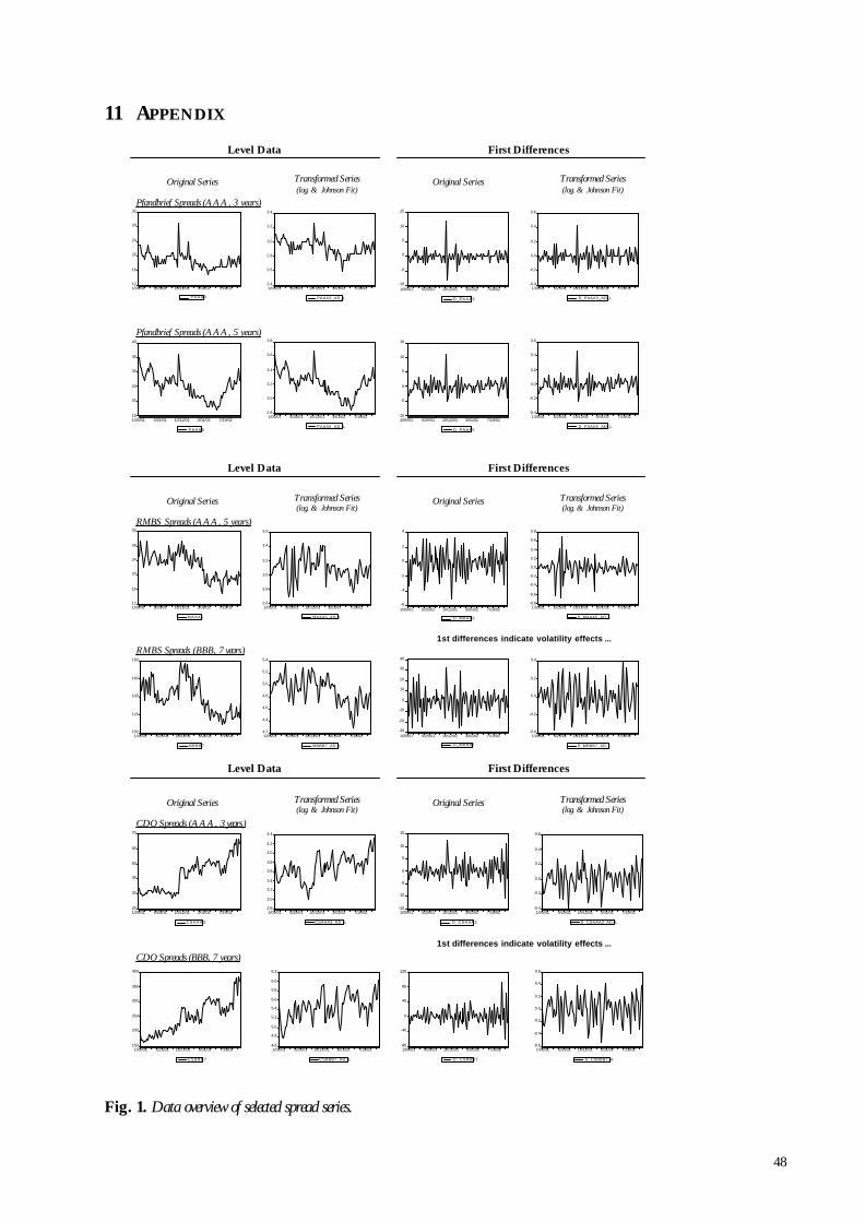
48

11 APPENDIX

Fig. 1. Data overview of selected spread series.

Pfandbrief Spreads (AAA, 3 years)

Original Series Transformed Series(log. & Johnson Fit)

12

16

20

24

28

32

1/05/01 5/25/01 10/12/01 3/01/02 7/19/02

P A A A 3

2.4

2.6

2.8

3.0

3.2

3.4

1/05/01 5/25/01 10/12/01 3/01/02 7/19/02

PAAA3_AD_L

-10

-5

0

5

10

15

1/05/01 5/25/01 10/12/01 3/01/02 7/19/02

D_PAAA3

-0.4

-0.2

0.0

0.2

0.4

0.6

1/05/01 5/25/01 10/12/01 3/01/02 7/19/02

D_PAAA3_AD_L

Pfandbrief Spreads (AAA, 5 years)

15

20

25

30

35

40

1/05/01 5/25/01 10/12/01 3/01/02 7/19/02

P A A A 5

2.8

3.0

3.2

3.4

3.6

3.8

1/05/01 5/25/01 10/12/01 3/01/02 7/19/02

PAAA5_AD_L

-10

-5

0

5

10

15

1/05/01 5/25/01 10/12/01 3/01/02 7/19/02

D_PAAA5

-0.4

-0.2

0.0

0.2

0.4

0.6

1/05/01 5/25/01 10/12/01 3/01/02 7/19/02

D_PAAA5_AD_L

Level Data First Differences

Original Series Transformed Series(log. & Johnson Fit)

RMBS Spreads (AAA, 5 years)

1st differences indicate volatility effects ...RMBS Spreads (BBB, 7 years )

12

16

20

24

28

32

1/05/01 5/25/01 10/12/01 3/01/02 7/19/02

MAAA5

-6

-4

-2

0

2

4

1/05/01 5/25/01 10/12/01 3/01/02 7/19/02

D_MAAA5

100

120

140

160

180

1/05/01 5/25/01 10/12/01 3/01/02 7/19/02

M B B B 7

-30

-20

-10

0

10

20

30

40

1/05/01 5/25/01 10/12/01 3/01/02 7/19/02

D_MBBB7

2.6

2.8

3.0

3.2

3.4

3.6

1/05/01 5/25/01 10/12/01 3/01/02 7/19/02

MAAA5_AD_L

-0.8

-0.6

-0.4

-0.2

0.0

0.2

0.4

0.6

0.8

1/05/01 5/25/01 10/12/01 3/01/02 7/19/02

D_MAAA5_AD_L

4.2

4.4

4.6

4.8

5.0

5.2

5.4

1/05/01 5/25/01 10/12/01 3/01/02 7/19/02

MBBB7_AD_L

-0.4

-0.2

0.0

0.2

0.4

1/05/01 5/25/01 10/12/01 3/01/02 7/19/02

D_MBBB7_AD_L

Original Series Transformed Series(log. & Johnson Fit)

Level Data First Differences

Original Series Transformed Series(log. & Johnson Fit)

CDO Spreads (AAA, 3 years )

1st differences indicate volatility effects ...

CDO Spreads (BBB, 7 years)

20

30

40

50

60

70

1/05/01 5/25/01 10/12/01 3/01/02 7/19/02

CSAAA3

150

200

250

300

350

400

1/05/01 5/25/01 10/12/01 3/01/02 7/19/02

C S B B B 7

2.8

3.0

3.2

3.4

3.6

3.8

4.0

4.2

4.4

1/05/01 5/25/01 10/12/01 3/01/02 7/19/02

CSAAA3_AD_L

4.6

4.8

5.0

5.2

5.4

5.6

5.8

6.0

6.2

1/05/01 5/25/01 10/12/01 3/01/02 7/19/02

CSBBB7_AD_L

-15

-10

-5

0

5

10

15

1/05/01 5/25/01 10/12/01 3/01/02 7/19/02

D_CSAAA3

-0.4

-0.2

0.0

0.2

0.4

0.6

1/05/01 5/25/01 10/12/01 3/01/02 7/19/02

D_CSAAA3_AD_L

-80

-40

0

40

80

120

1/05/01 5/25/01 10/12/01 3/01/02 7/19/02

D_CSBBB7

-0.6

-0.4

-0.2

0.0

0.2

0.4

0.6

1/05/01 5/25/01 10/12/01 3/01/02 7/19/02

D_CSBBB7_A

Original Series Transformed Series(log. & Johnson Fit)

Level Data First Differences

Original Series Transformed Series(log. & Johnson Fit)

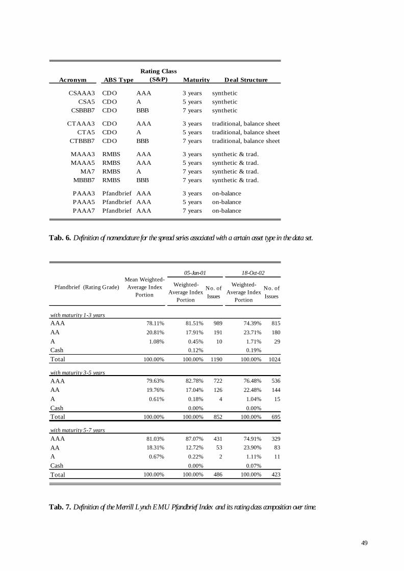
49

Tab. 6. Definition of nomenclature for the spread series associated with a certain asset type in the data set.

Tab. 7. Definition of the Merrill Lynch EMU Pfandbrief Index and its rating class composition over time.

Acronym ABS TypeRating Class

(S&P) Maturity Deal Structure

CSAAA3 CDO AAA 3 years syntheticCSA5 CDO A 5 years synthetic

CSBBB7 CDO BBB 7 years synthetic

CTAAA3 CDO AAA 3 years traditional, balance sheetCTA5 CDO A 5 years traditional, balance sheet

CTBBB7 CDO BBB 7 years traditional, balance sheet

MAAA3 RMBS AAA 3 years synthetic & trad.MAAA5 RMBS AAA 5 years synthetic & trad.

MA7 RMBS A 7 years synthetic & trad.MBBB7 RMBS BBB 7 years synthetic & trad.

PAAA3 Pfandbrief AAA 3 years on-balancePAAA5 Pfandbrief AAA 5 years on-balancePAAA7 Pfandbrief AAA 7 years on-balance

Weighted-Average Index

Portion

No. of Issues

Weighted-Average Index

Portion

No. of Issues

with maturity 1-3 yearsAAA 78.11% 81.51% 989 74.39% 815AA 20.81% 17.91% 191 23.71% 180A 1.08% 0.45% 10 1.71% 29Cash 0.12% 0.19%Total 100.00% 100.00% 1190 100.00% 1024

with maturity 3-5 yearsAAA 79.63% 82.78% 722 76.48% 536AA 19.76% 17.04% 126 22.48% 144A 0.61% 0.18% 4 1.04% 15Cash 0.00% 0.00%Total 100.00% 100.00% 852 100.00% 695

with maturity 5-7 yearsAAA 81.03% 87.07% 431 74.91% 329AA 18.31% 12.72% 53 23.90% 83A 0.67% 0.22% 2 1.11% 11Cash 0.00% 0.07%Total 100.00% 100.00% 486 100.00% 423

Mean Weighted-Average Index

Portion

05-Jan-01 18-Oct-02

Pfandbrief (Rating Grade)

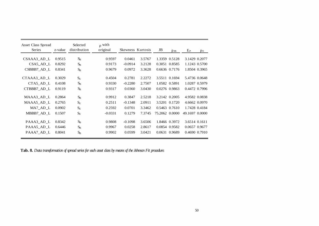
50

Tab. 8. Data transformation of spread series for each asset class by means of the Johnson Fit procedure.

Asset Class Spread Series z-value

Selected distribution

ρ with original Skewness Kurtosis JB p JB EP pE

CSAAA3_AD_L 0.9515 SB 0.9597 0.0461 3.5767 1.3359 0.5128 3.1429 0.2077CSA5_AD_L 0.8292 SB 0.9173 -0.0914 3.2128 0.3051 0.8585 1.1243 0.5700

CSBBB7_AD_L 0.8341 SB 0.9679 0.0972 3.3628 0.6636 0.7176 1.8504 0.3965

CTAAA3_AD_L 0.3029 SU 0.4504 0.2781 2.2272 3.5511 0.1694 5.4736 0.0648CTA5_AD_L 0.4108 SB 0.9330 -0.2280 2.7507 1.0582 0.5891 1.0287 0.5979

CTBBB7_AD_L 0.9119 SB 0.9317 0.0360 3.0430 0.0276 0.9863 0.4472 0.7996

MAAA3_AD_L 0.2864 SB 0.9912 0.3847 2.5218 3.2142 0.2005 4.9582 0.0838MAAA5_AD_L 0.2765 SU 0.2511 -0.1348 2.0911 3.5201 0.1720 4.6662 0.0970

MA7_AD_L 0.0902 SU 0.2592 0.0701 3.3462 0.5463 0.7610 1.7428 0.4184MBBB7_AD_L 0.1507 SU -0.0331 0.1279 7.3745 75.2062 0.0000 49.1697 0.0000

PAAA3_AD_L 0.8342 SB 0.9808 -0.1098 3.6506 1.8466 0.3972 3.6514 0.1611PAAA5_AD_L 0.6446 SB 0.9967 0.0258 2.8617 0.0854 0.9582 0.0657 0.9677PAAA7_AD_L 0.8041 SB 0.9902 0.0599 3.0421 0.0631 0.9689 0.4690 0.7910

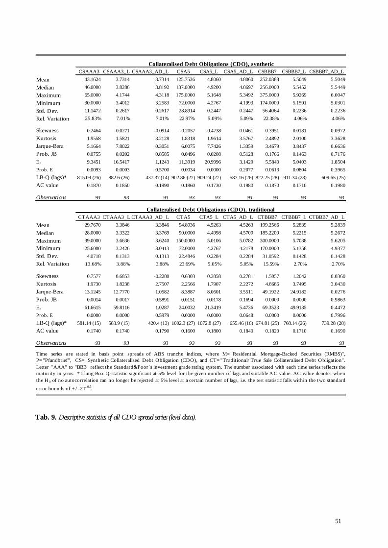
51

Tab. 9. Descriptive statistics of all CDO spread series (level data).

CSAAA3 CSAAA3_L CSAAA3_AD_L CSA5 CSA5_L CSA5_AD_L CSBBB7 CSBBB7_L CSBBB7_AD_L

Mean 43.1624 3.7314 3.7314 125.7536 4.8060 4.8060 252.0388 5.5049 5.5049

Median 46.0000 3.8286 3.8192 137.0000 4.9200 4.8697 256.0000 5.5452 5.5449

Maximum 65.0000 4.1744 4.3118 175.0000 5.1648 5.3492 375.0000 5.9269 6.0047

Minimum 30.0000 3.4012 3.2583 72.0000 4.2767 4.1993 174.0000 5.1591 5.0301

Std. Dev. 11.1472 0.2617 0.2617 28.8914 0.2447 0.2447 56.4064 0.2236 0.2236

Rel. Variation 25.83% 7.01% 7.01% 22.97% 5.09% 5.09% 22.38% 4.06% 4.06%

Skewness 0.2464 -0.0271 -0.0914 -0.2057 -0.4738 0.0461 0.3951 0.0181 0.0972Kurtosis 1.9558 1.5821 3.2128 1.8318 1.9614 3.5767 2.4892 2.0100 3.3628Jarque-Bera 5.1664 7.8022 0.3051 6.0075 7.7426 1.3359 3.4679 3.8437 0.6636Prob. JB 0.0755 0.0202 0.8585 0.0496 0.0208 0.5128 0.1766 0.1463 0.7176Ep 9.3451 16.5417 1.1243 11.3919 20.9996 3.1429 5.5840 5.0403 1.8504Prob. E 0.0093 0.0003 0.5700 0.0034 0.0000 0.2077 0.0613 0.0804 0.3965LB-Q (lags)* 815.09 (26) 882.6 (26) 437.37 (14) 902.86 (27) 909.24 (27) 587.16 (26) 822.25 (28) 911.34 (28) 609.65 (25)AC value 0.1870 0.1850 0.1990 0.1860 0.1730 0.1980 0.1870 0.1710 0.1980

Observations 93 93 93 93 93 93 93 93 93

CTAAA3 CTAAA3_L CTAAA3_AD_L CTA5 CTA5_L CTA5_AD_L CTBBB7 CTBBB7_L CTBBB7_AD_L

Mean 29.7670 3.3846 3.3846 94.8936 4.5263 4.5263 199.2566 5.2839 5.2839

Median 28.0000 3.3322 3.3769 90.0000 4.4998 4.5700 185.2200 5.2215 5.2672

Maximum 39.0000 3.6636 3.6240 150.0000 5.0106 5.0782 300.0000 5.7038 5.6205Minimum 25.6000 3.2426 3.0413 72.0000 4.2767 4.2178 170.0000 5.1358 4.9377Std. Dev. 4.0718 0.1313 0.1313 22.4846 0.2284 0.2284 31.0592 0.1428 0.1428Rel. Variation 13.68% 3.88% 3.88% 23.69% 5.05% 5.05% 15.59% 2.70% 2.70%

Skewness 0.7577 0.6853 -0.2280 0.6303 0.3858 0.2781 1.5057 1.2042 0.0360Kurtosis 1.9730 1.8238 2.7507 2.2566 1.7907 2.2272 4.8686 3.7495 3.0430Jarque-Bera 13.1245 12.7770 1.0582 8.3887 8.0601 3.5511 49.1922 24.9182 0.0276Prob. JB 0.0014 0.0017 0.5891 0.0151 0.0178 0.1694 0.0000 0.0000 0.9863Ep 61.6615 59.8116 1.0287 24.0032 21.3419 5.4736 69.3523 49.9135 0.4472Prob. E 0.0000 0.0000 0.5979 0.0000 0.0000 0.0648 0.0000 0.0000 0.7996LB-Q (lags)* 581.14 (15) 583.9 (15) 420.4 (13) 1002.3 (27) 1072.8 (27) 655.46 (16) 674.81 (25) 768.14 (26) 739.28 (28)AC value 0.1740 0.1740 0.1790 0.1600 0.1800 0.1840 0.1820 0.1710 0.1690

Observations 93 93 93 93 93 93 93 93 93

Collateralised Debt Obligations (CDO), synthetic

Collateralised Debt Obligations (CDO), traditional

Time series are stated in basis point spreads of ABS tranche indices, where M="Residential Mortgage-Backed Securities (RMBS)",P="Pfandbrief", CS="Synthetic Collateralised Debt Obligation (CDO), and CT="Traditional/True Sale Collateralised Debt Obligation".Letter "AAA" to "BBB" reflect the Standard&Poor`s investment grade rating system. The number associated with each time series reflects thematurity in years. * Llung-Box Q-statistic significant at 5% level for the given number of lags and suitable A C value. AC value denotes whenthe H0 of no autocorrelation can no longer be rejected at 5% level at a certain number of lags, i.e. the test statistic falls within the two standard

error bounds of +/-2T-0.5.

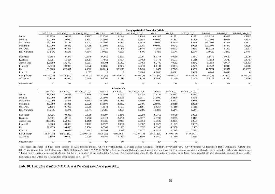
52

Tab. 10. Descriptive statistics of all MBS and Pfandbrief spread series (level data).

MAAA3 MAAA3_L MAAA3_AD_L MAAA5 MAAA5_L MAAA5_AD_L MA7 MA7_L MA7_AD_L MBBB7 MBBB7_L MBBB7_AD_LMean 20.7234 3.0217 3.0217 22.9782 3.1244 3.1244 65.1915 4.1751 4.1751 140.3138 4.9367 4.9367Median 22.0000 3.0910 2.9947 24.0000 3.1781 3.0854 66.0000 4.1897 4.1829 142.0000 4.9558 4.9514Maximum 25.0000 3.2189 3.2047 28.0000 3.3322 3.3879 75.0000 4.3175 4.3678 175.0000 5.1648 5.2871Minimum 17.0000 2.8332 2.7988 17.5000 2.8622 2.8285 60.0000 4.0943 4.0988 120.0000 4.7875 4.4829Std. Dev. 2.8099 0.1404 0.1404 3.2387 0.1446 0.1446 4.3854 0.0673 0.0673 16.9122 0.1207 0.1207Rel. Variation 13.56% 4.65% 4.65% 14.09% 4.63% 4.63% 6.73% 1.61% 1.61% 12.05% 2.44% 2.44%

Skewness -0.3854 -0.4277 -0.1348 -0.2056 -0.2931 0.0701 0.0774 0.0080 0.3847 0.1416 0.0127 0.1279Kurtosis 1.3751 1.3694 2.0911 1.4860 1.4694 3.3462 1.7472 1.6577 2.5218 1.8052 1.6713 7.3745Jarque-Bera 12.6680 13.2799 3.5201 9.6394 10.5222 0.5463 6.2409 7.0582 3.2142 5.9050 6.9174 75.2062Prob. JB 0.0018 0.0013 0.1720 0.0081 0.0052 0.7610 0.0441 0.0293 0.2005 0.0522 0.0315 0.0000Ep 53.6208 62.5617 4.6662 26.1014 32.9179 1.7428 11.2472 13.7045 4.9582 10.5874 13.2351 49.1697Prob. E 0 0 0.097 0 0 0.4184 0.0036 0.0011 0.0838 0.005 0.0013 0LB-Q (lags)* 886.74 (22) 905.08 (22) 164.22 (7) 934.77 (23) 967.94 (23) 35.073 (3) 752.65 (20) 785.63 (21) 645.58 (19) 699.72 (17) 733.1 (17) 22.393 (2)AC value 0.1710 0.1820 0.1270 0.1760 0.1810 0.1410 0.1890 0.1720 0.1760 0.1570 0.1890 0.1300

Observa t i ons 93 93 93 93 93 93 93 93 93 93 93 93

PAAA3 PAAA3_L PAAA3_AD_L PAAA5 PAAA5_L PAAA5_AD_L PAAA7 PAAA7_L PAAA7_AD_LMean 18.7766 2.9268 2.9268 24.9894 3.2045 3.2045 31.8192 3.4437 3.4437Median 19.0000 2.9444 2.9571 25.0000 3.2189 3.2111 31.5000 3.4499 3.4540Maximum 29.0000 3.3673 3.2652 36.0000 3.5835 3.6690 47.0000 3.8501 3.9766Minimum 15.0000 2.7081 2.5928 17.0000 2.8332 2.8406 22.0000 3.0910 2.9558Std. Dev. 2.1056 0.1065 0.1065 4.1543 0.1691 0.1691 5.8217 0.1819 0.1819Rel. Variation 11.21% 3.64% 3.64% 16.62% 5.28% 5.28% 18.30% 5.28% 5.28%

Skewness 1.4225 0.8305 -0.1098 0.1397 -0.2348 0.0258 0.3768 0.0708 0.0599Kurtosis 7.6301 4.9100 3.6506 2.6313 2.4766 2.8617 2.3737 2.0795 3.0421Jarque-Bera 115.6686 25.0950 1.8466 0.8381 1.9371 0.0854 3.7609 3.3975 0.0631Prob. JB 0.0000 0.0000 0.3972 0.6577 0.3796 0.9582 0.1525 0.1829 0.9689Ep 22.4233 10.8896 3.6514 0.5585 2.1983 0.0657 6.3592 4.2158 0.469Prob. E 0 0.0043 0.1611 0.7564 0.332 0.9677 0.0416 0.1215 0.791LB-Q (lags)* 151.67 (10) 189.51 (12) 226.06 (12) 415.8 (15) 459.52 (15) 410.94 (14) 584.97 (20) 617.95 (19) 543.62 (17)AC value 0.1940 0.0710 0.1090 0.1760 0.1820 0.1950 0.1810 0.1910 0.2130

Observa t i ons 93 93 93 93 93 93 93 93 93

Pfandbriefe

Mortgage-Backed Securities (MBS)

Time series are stated in basis point spreads of ABS tranche indices, where M="Residential Mortgage-Backed Securities (RMBS)", P="Pfandbrief", CS="Synthetic Collateralised Debt Obligation (CDO), andCT="Traditional/True Sale Collateralised Debt Obligation". Letter "AAA" to "BBB" reflect the Standard&Poor`s investment grade rating system. The number associated with each time series reflects the maturity in years.* Llung-Box Q-statistic significant at 5% level for the given number of lags and suitable AC value. AC value denotes when the H0 of no autocorrelation can no longer be rejected at 5% level at a certain number of lags, i.e. the

test statistic falls within the two standard error bounds of +/-2T -0.5.

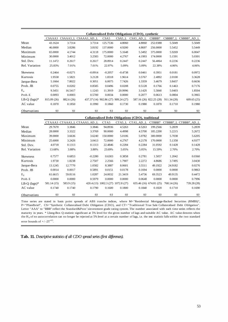
53

Tab. 11. Descriptive statistics of all CDO spread series (first differences).

CSAAA3 CSAAA3_L CSAAA3_AD_L CSA5 CSA5_L CSA5_AD_L CSBBB7 CSBBB7_L CSBBB7_AD_LMean 43.1624 3.7314 3.7314 125.7536 4.8060 4.8060 252.0388 5.5049 5.5049Median 46.0000 3.8286 3.8192 137.0000 4.9200 4.8697 256.0000 5.5452 5.5449Maximum 65.0000 4.1744 4.3118 175.0000 5.1648 5.3492 375.0000 5.9269 6.0047Minimum 30.0000 3.4012 3.2583 72.0000 4.2767 4.1993 174.0000 5.1591 5.0301Std. Dev. 11.1472 0.2617 0.2617 28.8914 0.2447 0.2447 56.4064 0.2236 0.2236Rel. Variation 25.83% 7.01% 7.01% 22.97% 5.09% 5.09% 22.38% 4.06% 4.06%

Skewness 0.2464 -0.0271 -0.0914 -0.2057 -0.4738 0.0461 0.3951 0.0181 0.0972Kurtosis 1.9558 1.5821 3.2128 1.8318 1.9614 3.5767 2.4892 2.0100 3.3628Jarque-Bera 5.1664 7.8022 0.3051 6.0075 7.7426 1.3359 3.4679 3.8437 0.6636Prob. JB 0.0755 0.0202 0.8585 0.0496 0.0208 0.5128 0.1766 0.1463 0.7176Ep 9.3451 16.5417 1.1243 11.3919 20.9996 3.1429 5.5840 5.0403 1.8504Prob. E 0.0093 0.0003 0.5700 0.0034 0.0000 0.2077 0.0613 0.0804 0.3965LB-Q (lags)* 815.09 (26) 882.6 (26) 437.37 (14) 902.86 (27) 909.24 (27) 587.16 (26) 822.25 (28) 911.34 (28) 609.65 (25)AC value 0.1870 0.1850 0.1990 0.1860 0.1730 0.1980 0.1870 0.1710 0.1980

Observations 93 93 93 93 93 93 93 93 93

CTAAA3 CTAAA3_L CTAAA3_AD_L CTA5 CTA5_L CTA5_AD_L CTBBB7 CTBBB7_L CTBBB7_AD_LMean 29.7670 3.3846 3.3846 94.8936 4.5263 4.5263 199.2566 5.2839 5.2839Median 28.0000 3.3322 3.3769 90.0000 4.4998 4.5700 185.2200 5.2215 5.2672Maximum 39.0000 3.6636 3.6240 150.0000 5.0106 5.0782 300.0000 5.7038 5.6205Minimum 25.6000 3.2426 3.0413 72.0000 4.2767 4.2178 170.0000 5.1358 4.9377Std. Dev. 4.0718 0.1313 0.1313 22.4846 0.2284 0.2284 31.0592 0.1428 0.1428Rel. Variation 13.68% 3.88% 3.88% 23.69% 5.05% 5.05% 15.59% 2.70% 2.70%

Skewness 0.7577 0.6853 -0.2280 0.6303 0.3858 0.2781 1.5057 1.2042 0.0360Kurtosis 1.9730 1.8238 2.7507 2.2566 1.7907 2.2272 4.8686 3.7495 3.0430Jarque-Bera 13.1245 12.7770 1.0582 8.3887 8.0601 3.5511 49.1922 24.9182 0.0276Prob. JB 0.0014 0.0017 0.5891 0.0151 0.0178 0.1694 0.0000 0.0000 0.9863Ep 61.6615 59.8116 1.0287 24.0032 21.3419 5.4736 69.3523 49.9135 0.4472Prob. E 0.0000 0.0000 0.5979 0.0000 0.0000 0.0648 0.0000 0.0000 0.7996LB-Q (lags)* 581.14 (15) 583.9 (15) 420.4 (13) 1002.3 (27) 1072.8 (27) 655.46 (16) 674.81 (25) 768.14 (26) 739.28 (28)AC value 0.1740 0.1740 0.1790 0.1600 0.1800 0.1840 0.1820 0.1710 0.1690

Observations 93 93 93 93 93 93 93 93 93

Collateralised Debt Obligations (CDO), synthetic

Collateralised Debt Obligations (CDO), traditional

Time series are stated in basis point spreads of ABS tranche indices, where M="Residential Mortgage-Backed Securities (RMBS)",P="Pfandbrief", CS="Synthetic Collateralised Debt Obligation (CDO), and CT="Traditional/True Sale Collateralised Debt Obligation".Letter "AAA" to "BBB" reflect the Standard&Poor`sinvestment grade rating system. The number associated with each time series reflects thematurity in years. * Llung-Box Q-statistic significant at 5% level for the given number of lags and suitable AC value. AC value denotes whenthe H 0 of no autocorrelation can no longer be rejected at 5% level at a certain number of lags, i.e. the test statistic falls within the two standard

error bounds of +/-2T-0.5.

Working Paper Series: Finance & Accounting

No.120: Baris Serifsoy/ Marco Weiss, Efficient Systems for the Securities Transaction Industry- A Framework for the European Union, November 2003

No.119: Andreas Jobst, Verbriefung und ihre Auswirkung auf die Finanzmarktstabilität, October 2003

No.118: Reinhard H. Schmidt, Corporate Governance in Germany: An Economic Perspective, August 2003 (erscheint in: “The German Financial System”, Krahnen, J.P. und Schmidt, R.H. (Hrsg.), Kapitel 12, Oxford University Press, London (2004))

No.117: Volker Laux, The Ignored Performance Measure, October 2003

No.116: Christian Gaber, Project Selection, Income Smoothing, and Bayesian Learning, September 2003

No.115: Hergen Frerichs/ Mark Wahrenburg, Evaluating internal credit rating systems depending on bank size, September 2003

No.114: Raimond Maurer/ Frank Reiner/ Ralph Rogalla, Risk and Return of Open-End Real-Estate Funds: The German Case, September 2003

No.113: Patrick Behr/ André Güttler/ Thomas Kiehlborn, Der deutsche Hypotheken-bankenmarkt: Ergebnisse einer empirischen Untersuchung, September 2003 (erschienen in: Die Bank, Heft 8/2003, unter den Titeln „Hypothekenbanken: Die Zukunft liegt im Firmengeschäft“ und „Internationalisierungsstategien deutscher Hypothekenbanken: Die Zukunft liegt im Ausland“; erscheint in: Immobilien & Finanzierung)

No.112: Reinhard H. Schmidt/ Andreas Hackethal/ Valentin Marinov, Die Banken-märkte Russlands und Bulgariens, July 2003 (erschienen in: Die Bank, Heft 4/2003 und Heft 8/2003)

No.111: Reinhard H. Schmidt/ Marcel Tyrell, What constitutes a financial system in general and the German financial system in particular?, July 2003 (erscheint in: “The German Financial System”, Krahnen, J.P. und Schmidt, R.H. (Hrsg.), Kapitel 2, Oxford University Press, London (2004))

No.110: Falko Fecht, On the Stability of Different Financial Systems, June 2003

No.109: Raimond Maurer/ Shohreh Valiani, Hedging the Exchange Rate Risk in International Portfolio Diversification: Currency Forwards versus Currency Options, June 2003

No.108: Raimond Maurer/ Frank Reiner/ Steffen Sebastian, Financial Characteristics of International Real Estate Returns: Evidence from the UK, US, and Germany, May 2003

No.107: Anne d’Arcy/ Michiyo Mori/ Christine Rossbach, The impact of valuation rules for intangible assets in Japanese and German accounts of listed companies, April 2003

No.106: Andreas Hackethal, German banks – a declining industry?, March 2003 (erscheint in: “The German Financial System”, Krahnen, J.P. und Schmidt, R.H. (Hrsg.), Kapitel 3, Oxford University Press, London (2004))

No.105: Ingo E. Tschach, The long term impact of microfinance on income, wages and the sectoral distribution of economic activity, April 2003

No.104: Reinhard H. Schmidt/ Marco Weiß, Shareholder vs. Stakeholder: Ökonomische Fragestellungen, January 2003 (erscheint in: “Handbuch Corporate Governance”, Hommelhoff, P., Hopt, K. und A. v. Werder (Hrsg.))

No.103: Ingo E. Tschach, The Theoretical Derivation of Credit Market Segmentation as the Result of a Free Market Process, March 2003

No.102: Samuel Lee/ Nina Moisa/ Marco Weiss, Open Source as a Signalling Device – An Economic Analysis, March 2003

No.101: Christian Gaber, Bewertung von Fertigerzeugnissen zu Voll- oder Teilkosten? Ansatz von Forderungen zum Nennwert oder Barwert? Eine agencytheoretische Analyse zur zielkongruenten Performancemessung, December 2002

No.100: Oliver Ruß / Günther Gebhardt, Erklärungsfaktoren für den Einsatz von Währungsderivaten bei deutschen Unternehmen – eine empirische Logit-Analyse, August 2002

No.99: Christian Gaber, Gewinnglättung und Steuerung dezentraler Investitions-entscheidungen bei sich gegenseitig ausschließenden Investitionsprojekten, September 2002

No.98: Volker Laux, On the Value of Influence Activities for Capital Budgeting, September 2002

No.97: Gunter Löffler, Avoiding the rating bounce: Why rating agencies are slow to react to new information, June 2002

No.96: Andreas A. Jobst, Collateralized Loan Obligations (CLOs) – A Primer, December 2002

No.95: Günther Gebhardt/ Rolf Reichardt/ Carsten Wittenbrink, Accounting for Financial Instruments in the Banking Industry, November 2002

No.94: Ulf Herold/ Raimond Maurer, Portfolio choice and estimation risk – A comparison of Bayesian approaches to resampled efficiency, June 2002

No.93: Olivia S. Mitchell/ David McCarthy, Annuities for an Ageing World, June 2002

No.92: Ulf Herold/ Raimond Maurer, How much foreign stocks? Classical versus Bayesian approaches to asset allocation, June 2002

No.91: Gunter Löffler/ Patrick F. Panther/ Erik Theissen, Who Knows What When? – The Information Content of Pre-IPO Market Prices, June 2002

No.90: Reinhard Hujer/ Sandra Vuletic/ Stefan Kokot, The Markov switching ACD model, April 2002

No.89: Markus C. Arnold/ Robert M. Gillenkirch, Stock Options as Incentive Contracts and Dividend Policy, April 2002

No.88: Anne d'Arcy/ Sonja Grabensberger, The Quality of Neuer Markt Quarterly Reports - an Empirical Investigation, January 2002

No.87A: Reinhard H. Schmidt /Ingo Tschach, Microfinance as a Nexus of Incentives, May 2001

No.87: Reinhard H. Schmidt/ Ingo Tschach, Microfinance als ein Geflecht von Anreizproblemen, Dezember 2001 (erscheint in den Schriften des Vereins für Socialpolitik, 2002)

No.86: Ralf Elsas/ Yvonne Löffler, Equity Carve-Outs and Corporate Control in Germany, December 2001

No.85: Günther Gebhardt/ Stefan Heiden/ Holger Daske, Determinants of Capital Market Reactions to Seasoned Equity Offers by German Corporations, December 2001

No.84: Hergen Frerichs/ Gunter Löffler, Evaluating credit risk models: A critique and a proposal, October 2001 (erschienen in: Journal of Risk, 5, 4, Summer 2003, 1-23)

No. 83: Ivica Dus/ Raimond Maurer, Integrated Asset Liability Modelling for Property Casuality Insurance: A Portfolio Theoretical Approach, October 2001 (erscheint in Handbuch Asset-Liability Management, hrsg. von M. Rudolph u.a.)

No.82: Raimond Maurer/ Frank Reiner, International Asset Allocation with Real Estate Securities in a Shortfall-Risk Framework: The Viewpoint of German and US Investors, September 2001

No.81: Helmut Laux, Das Unterinvestitionsproblem beim EVA-Bonussystem, August 2001

No.80: Helmut Laux, Bedingungen der Anreizkompatibilität, Fundierung von Unter-nehmenszielen und Anreize für deren Umsetzung, July 2001

No. 79: Franklin Allen/ Douglas Gale, Banking and Markets, July 2001

No.78: Joachim Grammig/ Michael Melvin/ Christian Schlag, Price Discovery in International Equity Trading, July 2001 (erscheint in: Journal of Empirical Finance unter dem Titel “Internationally Cross-Listed Stock Prices During Overlapping Trading Hours: Price Discovery and Exchange Rate Effects”)

No.77: Joachim Grammig/ Reinhard Hujer/ Stefan Kokot, Tackling Boundary Effects in Nonparametric Estimation of Intra-Day Liquidity Measures, July 2001

No.76: Angelika Esser/ Christian Schlag , A Note on Forward and Backward Partial Differential Equations for Derivative Contracts with Forwards as Underlyings, June 2001 (erschienen in “Foreign Exchange Risk”, Hakala, J.; Wystup, U. (eds), 2002, 115-124)

No.75: Reinhard H. Schmidt/ Marcel Tyrell/ Andreas Hackethal, The Convergence of Financial Systems in Europe, May 2001 (erschienen in: German Financial Markets and Institutions: Selected Studies, Special Issue 1-02 of Schmalenbach Business Review (2002), S. 7-53)

No.74: Ulf Herold, Structural positions and risk budgeting - Quantifying the impact of structural postions and deriving implications for active portfolio management, May 2001

No.73: Jens Wüstemann, Mängel bei der Abschlußprüfung: Tatsachenberichte und Analyse aus betriebswirtschaftlicher Sicht, April 2001 (erschienen in: „Der Wirtschaftsprüfer als Element der Corporate Governance“, Zentrum für Europäisches Wirtschaftsrecht, Bonn 2001, S. 25-60)

No.72: Reinhard H. Schmidt, The Future of Banking in Europe, March 2001 (erschienen in: Financial Markets and Portfolio Management, Vol. 15 (2001), S. 429-449)

No.71: Michael H. Grote/ Britta Klagge, Wie global sind Japans Banken? Die Ver-änderung institutioneller Bedingungen und ihre Auswirkungen auf die internationale Präsenz japanischer Kreditinstitute, April 2001

No.70: Stefan Feinendegen/ Eric Nowak, Publizitätspflichten börsennotierter Aktien-gesellschaften im Spannungsfeld zwischen Regelberichterstattung und Ad-hoc-Publizität - Überlegungen zu einer gesetzeskonformen und kapitalmarktorientierten Umsetzung, März 2001 (erscheint in: Die Betriebswirtschaft)

No.69: Martin F. Grace/ Robert W. Klein/ Paul R. Kleindorfer, The Demand for Homeowners Insurance with Bundled Catastrophe Coverages, March 2001

No.68: Raimond Maurer/ Martin Pitzer/ Steffen Sebastian, Konstruktion transaktions-basierter Immobilienindizes: Theoretische Grundlagen und empirische Umsetzung für den Wohnungsmarkt in Paris, Februar 2001

No.67: Gyöngyi Bugár/ Raimond Maurer, International Equity Portfolios and Currency Hedging: The Viewpoint of German and Hungarian Investors, February 2001 (erscheint in. ASTIN-Bulletin)

No.66: Rainer Brosch, Portfolio-aspects in real options management, February 2001

No.65a: Marcel Tyrell/ Reinhard H. Schmidt, Pension Systems and Financial Systems in Europe:A Comparison from the Point of View of Complementarity, July 2001 (erschienen in ifo-Studien, Vol. 47, 2001, S. 469-503)

No.65: Marcel Tyrell/ Reinhard H. Schmidt, Pensions- und Finanzsysteme in Europa: Ein Vergleich unter dem Gesichtspunkt der Komplementarität, Februar 2001 (erschienen in gekürzter Fassung in: „Private Versicherung und Soziale Sicherung“, Festschrift zum 60. Geburtstag von Prof. Dr. Dr. h.c. Roland Eisen, hrsg. von H.-C. Mager, H. Schäfer, K. Schrüfer, Metropolis: Marburg),

No.64: Jutta Dönges/ Frank Heinemann, Competition for Order Flow as a Coordination Game, January 2001

No.63: Eric Nowak/ Alexandra Gropp, Ist der Ablauf der Lock-up-Frist bei Neu-emissionen ein kursrelevantes Ereignis, Dezember 2000 (erschienen in Zeitschrift für betriebswirtschaftliche Forschung, Februar 2002)

No.62: Ulrich Kaiser/ Andrea Szczesny, Einfache ökonometrische Verfahren für die Kreditrisikomessung: Verweildauermodelle, Dezember 2000

No.61: Ulrich Kaiser/ ndrea Szczesny, Einfache ökonometrische Verfahren für die Kreditrisikomessung: Logit- und Probit-Modelle, Dezember 2000

No.60: Andreas Hackethal, How Unique Are US Banks? - The Role of Banks in Five Major Financial Systems, December 2000 (erschienen in: Zeitschrift für Nationalökonomie und Statistik, Vol. 221, S. 592-619)

No.59: Rolf Elgeti/ Raimond Maurer, Zur Quantifizierung der Risikoprämien deutscher Versicherungsaktien im Kontext eines Multifaktorenmodells, Oktober 2000 (erschienen in: Zeitschrift für die gesamte Versicherungswissenschaft 4/2000, S. 577- 603.)

No.58: Harald A. Benink/ Reinhard H. Schmidt, Towards a Regulatory Agenda for Banking in Europe, September 2000 (erschienen in: Research in Financial Services-Bank Crises: Causes, Analysis and Prevention, Vol.12, JAI Press-Elsevier Science, hrsg. von George G. Kaufman, 2000)

No.57: Thomas G. Stephan/ Raimond Maurer/ Martin Dürr, A Multiple Factor Model for European Stocks, September 2000

No.56: Martin Nell/ Andreas Richter, Catastrophe Index-Linked Securities and Reinsurance as Substituties, August 2000

No.55: Four short papers on Development Finance, August 2000

Reinhard H. Schmidt, Entwicklungsfinanzierung; (erschienen in: Handwörterbuch des Bank- und Finanzwesens, 3. Aufl., hrsg. von Wolfgang Gerke und Manfred Steiner, Stuttgart: Schäffer-Poeschel, 2001)

Reinhard H. Schmidt, Banking Regulation contra Microfinance; (erschienen in: Savings and Development, Vol. 24 (2000) , S.111-121.)

Ingo Tschach, The Impact of Inflation on Long-Term Housing Loans;

Eva Terberger-Stoy/ Marcel Tyrell/ Joseph E. Stiglitz (erschienen in: Entwick-lung und Zusammenarbeit, 41. Jahrgang (2000), S. 46-49)

No.54: Raimond Maurer/ Thomas G. Stephan, Vermögensanlagevorschriften für deutsche Versicherungsunternehmen: Status Quo und finanzwirtschaftliche Bewertungen, Juli 2000 (erschienen in: Handbuch Spezialfonds (hrsg. von J.M. Kleeberg und C. Schlenger), Bad Soden 2000, S. 143-176.)

No.53: Joachim Grammig/ Reinhard Hujer/Stefan Kokot, Bias-free Nonparametric Estimation of Intra-Day Trade Activity Measures, June 2000

No.52: Raimond Maurer/ Steffen Sebastian/ Thomas G. Stephan, Immobilienindizes im Portfolio-Management, Mai 2000 (erscheint in Deutscher Aktuarverein (Hrsg.): Investmentmodelle für das Asset-Liability-Modelling von Versicherungs-unternehmen, 2002)

No.51: Raimond Maurer/ Steffen Sebastian, Inflation Risk Analysis of European Real Estate Securities, Mai 2000 (erscheint in: Journal of Real Estate Research, 2002)

No.50: Andreas Hackethal/ Reinhard H. Schmidt, Finanzsysteme und Komplemen-tarität, April 2000 ( erschienen in: Kredit und Kapital, Beiheft 15 "Neue finanzielle Arrangements: Märkte im Umbruch", 2000, S. 53-102)

No.49: Mark Wahrenburg/ Susanne Niethen, Vergleichende Analyse alternativer Kredit-risikomodelle, April 2000 (erschienen in: Kredit und Kapital, Heft 2, 2000)

No.48: Christian Leuz, IAS versus US GAAP: A "New Market" Based Comparsion, January 2000 (erschienen in: Journal of Accounting Research, 41 (2003), S. 445-472)

No.47: Ralf Elsas/ Mahmoud El-Shaer/ Erik Theissen, Beta and Returns Revisited – Evidence from the German Stock Market, December 1999 (erschienen in: Journal of International Financial Markets, Institutions and Money 13 (2003), 1-18)

No.46: Michael H. Grote/ Sofia Harrschar-Ehrnborg/ Vivien Lo, Technologies and Proximities: Frankfurt´s New Role in the European Financial Centre System, December 1999

No.45: Reinhard H. Schmidt/ Adalbert Winkler, Building Financial Institutions in Developing Countries, November 1999 (erschienen in: "Journal für Entwicklungspolitik", XVI/3, 2000, S. 329-346)

No.44: Konstantin Korolev/ Kai D. Leifert/ Heinrich Rommelfanger, Arbitragetheorie bei vagen Erwartungen der Marktteilnehmer, November 1999

No.43: Reinhard H. Schmidt/ Stefanie Grohs, Angleichung der Unternehmensverfassung in Europa –Ein Forschungsprogramm, November 1999 (erschienen in: Systembildung und Systemlücken in Kerngebieten des Europäischen Privatrechts, hrsg. von Stefan Grundmann, Tübingen: Mohr Siebeck, 2000, S. 146-188)

No.42: Konstantin Kovolev/ Kai D. Leifert/ Heinrich Rommelfanger, Optionspreis-theorie bei vagen Daten, Oktober 1999

No.41: Christian Leuz/ Robert E. Verrecchia, The Economic Consequences of Increased Disclosure, June 2000 (erschienen in: Journal of Accounting Research 38 (Supplement 2000), 91-124)

No.40: Christian Leuz, The Development of Voluntary Cash Flow Statements in Germany and the Influence of International Reporting Standards, July 1999 (erschienen in: Schmalenbach Business Review, Vol. 52 (2) (April 2000), S. 182-207)

No.39: Ulrike Stefani, Quasirenten, Prüferwechsel und rationale Adressaten, Juni 1999

No.38: Michael Belledin/ Christian Schlag, An Empirical Comparison of Alternative Stochastic Volatility Models, June 1999

No.37: Jens Wüstemann, Internationale Rechnungslegungsnormen und neue Institutionen-ökonomik, Mai 1999

No.36: Robert Gillenkirch/ Matthias M. Schabel, Die Bedeutung der Periodenerfolgs-rechnung für die Investitionssteuerung – Der Fall ungleicher Zeitpräferenzen, April 1999 (die überarbeitete Fassung "Investitionssteuerung, Motivation und Periodenerfolgsrechnung bei ungleichen Zeitpräferenzen" erscheint voraussichtlich 2001 in der ZfbF)

No.35: Reinhard H. Schmidt, Differences between Financial Systems in Europe: Consequences for EMU, April 1999 (erschienen in "The Monetary Transmission Mechanism: Recent Developments and Lessous for Europe", hrsg. v. Deutsche Bundesbank, Houndsmill (UK), 2001, S. 208-240)

No.34: Theodor Baums/ Erik Theissen, Banken, bankeigene Kapitalanlagegesellschaften und Aktienemissionen, März 1999 (erschienen in: Zeitschrift für Bankrecht und Bankwirtschaft, 11 (1999), Heft 3, S. 125-134)

No.33: Andreas Hackethal/ Reinhard H. Schmidt, Financing Patterns: Measurement Concepts and Empirical Results, May 2000

No.32: Michael H. Haid/ Eric Nowak, Executive compensation and the susceptibility of firms to hostile takeovers – An empirical investigation of the U.S. oil industry, March 1999

No.31: Reinhard H. Schmidt/ Jens Maßmann, Drei Mißverständnisse zum Thema "Shareholder Value", Februar 1999 (erschienen in Kumar/ Osterloh/ Schreyögg (Hrsg.):Unternehmensethik und die Transformation des Wettbewerbs, Festschrift für Professor Dr. Dr. h. c. Horst Steinmann zum 65. Geburtstag,1999, Schäffer-Poeschel Verlag Stuttgart, S.125-157 )

No.30: Eberhard Feess/ Michael Schieble, Credit Scoring and Incentives for Loan Officers in a Principal Agent Model, January 1999

No.29: Joachim Grammig/ Dirk Schiereck/ Erik Theissen, Informationsbasierter Aktien-handel über IBIS, Januar 1999 (erschienen in: Zeitschrift für betriebswirtschaftlicher Forschung 52 (2000), 619-642)

No.28: Ralf Ewert/ Eberhard Feess/ Martin Nell, Auditor Liability Rules under Imperfect Information and Costly Litigation – The Welfare Increasing Effect of Liability Insurance, January 1999 (erschienen in: European Accounting Review)

No.27: Reinhard H. Schmidt/ Gerald Spindler, Path Dependence, Corporate Governance and Complementarity, March 2000 (erschienen in: International Finance, Vol. 5 (2002), No. 4, S. 311-333; erscheint in: Jeffrey Gordon & Mark Roe, eds.: Convergence and Rersistence of Corporate Governance Systems, University of Chicago Press, 2001)

No.26: Thorsten Freihube/ Carl-Heinrich Kehr/ Jan P. Krahnen/ Erik Theissen, Was leisten Kursmakler? Eine empirische Untersuchung am Beispiel der Frankfurter Wertpapierbörse, Dezember 1998 (erschienen in: Kredit und Kapital 32(1999), Heft3, S. 426-460)

No. 25: Jens Maßmann/ Reinhard H. Schmidt, Recht, internationale Unternehmensstra-tegien und Standortwettbewerb, December 1998 (erschienen in: Jahrbuch für Neue Politische Ökonomie, Band 18, hrsg. von K.-E. Schenk u.a., Tübingen 2000, S. 169-204)

No. 24: Eberhard Feess/ Martin Nell, The Manager and the Auditor in a Double Moral Hazard Setting: Efficiency through Contingent Fees and Insurance Contracts, December 1998

No. 23: Carl-Heinrich Kehr/ Jan P. Krahnen/ Erik Theissen, The Anatomy of a Call Market: Evidence from Germany, December 1998 (erschienen in: Journal of Financial Intermediation 10 (2001), S. 249-270)

No. 22: Christian K. Muus, Non-voting shares in France: An empirical analysis of the voting premium, December 1998

No. 21: Christian Leuz, Voluntary Disclosure of Cash Flow Statements and Segment Data in Germany, September 1998 (erscheint in: The Economics and Politics of Accounting: International Essays, C. Leuz, D. Pfaff and A. Hopwood (eds), Oxford University Press)

No. 20: Anne D`Arcy, The Degree of Determination of National Accounting Systems – An Empirical Investigation, September 1998

No. 19: Helmut Laux, Marktwertmaximierung und CAPM im Ein- und Mehrperioden-Fall, September 1998 (erschienen in Unternehmensführung, Ethik und Umwelt, Festschrift zum 65. Geburtstag von Hartmut Kreikebaum, hrsg. von Gerd-Rainer Wagner, Wiesbaden 1999, S. 226-251)

No. 18: Joachim Grammig/ Reinhard Hujer/ Stefan Kokot/ Kai-Oliver Maurer, Ökonometrische Modellierung von Transaktionsintensitäten auf Finanzmärkten; Eine Anwendung von Autoregressive Conditional Duration Modellen auf die IPO der Deutschen Telekom, August 1998

No. 17: Hanne Böckem, An Investigation into the Capital Market Reaction on Accounting Standards Enforcement, July 1998

No. 16: Erik Theissen, Der Neue Markt: Eine Bestandsaufnahme, April 1998 (erschienen in: Zeitschrift für Wirtschafts- und Sozialwissenschaften, Heft 4/98, S. 623-652)

No. 15: Jan Pieter Krahnen, Finanzierungstheorie: Ein selektiver Überblick, April 1998 (englische Fassung erschienen in "Gutenberg Centennial", hrsg. von Horst Albach, Berlin, 2000)

No. 14: Erik Theissen, Liquiditätsmessung auf experimentellen Aktienmärkten, April 1998 (erschienen in: Kredit und Kapital, 32(1999), Heft 2, S. 225-264)

No. 13: Reinhard H. Schmidt, Erich Gutenberg und die Theorie der Unternehmung, February 1998 (englische Fassung erschienen in "Theory of the Firm", hrsg. von Horst Albach u.a., Berlin 2000, S. 3-39)

No. 12: Adalbert Winkler, Financial Development, Economic Growth and Corporate Governance, February 1998 (erschienen in: Asian Financial Markets, hrsg. von Lukas Menkhoff/Beate Reszat, Baden-Baden 1998, S. 15-44)

No. 11: Andreas R. Hackethal/ Marcel Tyrell, Complementarity and Financial Systems – A Theoretical Approach, December 1998

No. 10: Reinhard H. Schmidt/ Andreas Hackethal/ Marcel Tyrell, Disintermediation and the Role of Banks in Europe: An International Comparison, January 1998 (erschienen in: Journal of Financial Intermediation, Vol. 8, 1999, S.37-67)

No. 9: Stefan Heiden/ Günther Gebhardt/ Irmelin Burkhardt, Einflußfaktoren für Kurs-reaktionen auf die Ankündigung von Kapitalerhöhungen deutscher Aktiengesellschaften, December 1997

No. 8: Martin Nell, Garantien als Signale für die Produktqualität?, November 1997 (erscheint in: Zeitschrift für betriebswirtschaftliche Forschung)

No. 7: Robert M. Gillenkirch, Anreizwirkungen und Bewertung von Erfolgsbeteili-gungen im Portefeuillemanagement, November 1997 (erschienen in: ZfB, Sonderheft Finanzmanagement 1999)

No. 6: Reinhard H. Schmidt/ C.-P. Zeitinger, Critical Issues in Microbusiness Finance and the Role of Donors, October 1997 (erschienen in: Strategic Issues in Microfinance, ed. by Kimenyi/Wieland/Von Pischke, Averbury, UK, 1998, S. 27-51)

No. 5: Erik Theissen/ Mario Greifzu, Performance deutscher Rentenfonds, September 1997 (erschienen in: Zeitschrift für betriebswirtschaftliche Forschung, 50. Jg., 1998, S. 436-461)

No. 4: Jan Pieter Krahnen/ Martin Weber, Marketmaking in the Laboratory: Does Competition Matter?, September 1997

No. 3: Reinhard H. Schmidt, Corporate Governance: The Role of Other Constituen-cies, July 1997 (erschienen in: Pezard, Alice;Thiveaud, Jean-Marie (Hrsg.): Corporate Governance: Cross Border Experience, Paris, 1997, S. 61-74)

No. 2: Ralf Ewert/ Christian Ernst, Strategic Management Accounting, Coordination and Long-term Cost Structure, July 1997 (erschienen unter dem Titel "Target Costing, Coordination and Strategic Cost Management" in Euopean Accounting Review, Vol.8, No.1 (1999), S. 23-49)

No. 1: Jan P. Krahnen/ Christian Rieck/ Erik Theissen, Insider Trading and Portfolio Structure in Experimental Asset Markets with a Long Lived Asset, July 1997 (erschienen in European Journal of Finance, Vol. 5, Nr. 1, March 1999, S. 29-50)

Kontaktadresse für Bestellungen:

Professor Dr. Reinhard H. Schmidt Wilhelm Merton Professur für

Internationales Bank- und Finanzwesen Mertonstr. 17

Postfach 11 19 32 / HPF66 D-60054 Frankfurt/Main

Tel.: +49-69-798-28269 Fax: +49-69-798-28272

e-mail: rschmidt@wiwi.uni- frankfurt.de http://www.finance.uni-frankfurt.de/index.php?lg=&men=4&case=wp

Mit freundlicher Unterstützung der Unternehmen der Sparkassen-Finanzgruppe Hessen-Thüringen.