1 Copyright © 2009 by ASME

Proceedings of the ASME 2009 International Design Engineering Technical Conferences & Computers and Infor-mation in Engineering Conference

IDETC/CIE 2009 August 30 - September 2, 2009, San Diego, California, USA

DRAFT DETC2009-86449

MBS SOFTWARE DEVELOPMENT WITH MATLAB FOR TEACHING AND INDUSTRIAL USAGES

Javier García de Jalón Universidad Politécnica de Madrid Dep. de Mat. Aplicada and INSIA

José Gutiérrez Abascal 2 28006 Madrid, Spain

Phone: 34-913363213 E-mail: javier.garciadejalon@upm.es

Andrés F. Hidalgo Universidad Politécnica de Madrid

INSIA (Campus Sur UPM) Carretera de Valencia, km.7

28031 Madrid, Spain Phone: 34-913365335

E-mail: andres.francisco.hidalgo@upm.es

Alfonso Callejo Universidad Politécnica de Madrid

INSIA (Campus Sur UPM) Carretera de Valencia, km.7

28031 Madrid, Spain Phone: 34-913365335

E-mail: a.callejo@alumnos.upm.es

ABSTRACT

In this article, two formulations implemented in Matlab™ for the dynamic simulation of multibody systems are described. The developed framework allows a rapid development of pro-grams and a clean implementation of algorithms, offering many aids to make the data pre and post-process. However, Matlab is not efficient at all when working with small matrices, as hap-pens with multibody systems.

This work describes a global formulation and a topologic (semi-recursive) formulation. Both are applied to two real, medium-large cases: an automobile and a semi-trailer truck. In both cases the pure Matlab results are presented, and also the improvements which can be achieved when some of the func-tions are programmed in C/C++ and are executed as MEX-functions. It can be proved that execution times can be lowered between one and two orders of magnitude, beating those of some commercial programs.

1 INTRODUCTION Matlab is a scientific programming language which includes an IDE (Integrated Development Environment) and is profusely used in many universities and high tech companies. Some of its advantages are a very compact and straightforward representa-tion of algorithms, the ability of allowing a very fast implemen-tation and debugging of numerical procedures, an excellent numerical library, an extensive set of toolboxes and many fa-cilities for simple pre and post-processing works. These charac-teristics allow easy software prototype development, fast com-parison of formulations and easy evaluation of numerical errors and instabilities. It seems that Matlab should be a very appro-priate tool to develop multibody simulation programs. This is true for small examples written for educational purposes, but not for industrial applications in medium or large problems.

Experience shows that Matlab is very slow in some kind of programs, for instance when using small matrices, as it happens with multibody recursive formulations. Matlab is much more efficient with finite element computations than with multibody systems. The main reason is the greater relative weight of code against arithmetic operations.

The development of multibody simulation software using Mat-lab with teaching purposes [3] presents no problems, because algorithms and their different variations are shown clearly and execution times are very small, as common teaching examples are also small.

However, when practical, large problems are faced with the same Matlab programs, those execution times can become completely unacceptable. Provided that Matlab’s practical ad-vantages (versatility, ease of data change, possibility to obtain results of nearly any type almost on the way, etc.) also have a great interest in real, big problems, it is important to study and assess the improvements obtained by programming the critical functions in C/C++, both for global and topologic multibody formulations.

In this article two dynamic formulations for multibody systems are described: a global one based on natural coordinates [1], and a topological one based on a semi-recursive formulation which is simple and efficient [2].

As corresponding examples for real, large problems, two vehi-cles have been selected: a 15 dof car (with McPherson front suspension and multi-link rear suspension) and a 39 dof and 5 axles truck (with rigid axles suspension, leaf springs and pneu-matic springs).

According to the recommendations to improve efficiency in-cluded in the Matlab documentation, the use of MEX-functions

2 Copyright © 2009 by ASME

is the most important technique. This paper presents this im-provement for both global and topological multibody formula-tions.

2 MBS SOFTWARE IMPLEMENTED WITH MATLAB Matlab, as a programming environment (IDE), is much more adequate for finite element method programming than for mul-tibody systems dynamics programming. This is mainly because of the size of the matrices, which is much larger in finite ele-ment method problems.

As an example, there is only one multibody systems simulation commercial program, SimMechanics™, which is considered adequate only for small problems. In February 2009 a search with the keywords “finite element” in Matlab’s user community (www.mathworks.com/matlabcentral/fileexchange) returned 55 programs, while a search with “multibody” only returned 2 results (one of them related with SimMechanics).

However, the results presented in this paper demonstrate that Matlab, with certain functions programmed in C/C++ as MEX-functions, makes it possible to obtain excellent results, specifi-cally when using the semi-recursive topologic formulation.

2.1 Implementing a global formulation Historically, the first practical systems studied in the sixties (spacecraft and robots) were open-chain systems. Therefore, relative coordinates were more appropriate than Cartesian co-ordinates. In addition to this, relative coordinates had fewer storage requirements and this was important for the computers of that time. In the seventies and eighties the main emphasis switched to automobile applications, which are inherently closed-chain systems. As a consequence, software packages that used highly constrained Cartesian coordinates, such as ADAMS and DADS, were developed. These programs are based on global formulations, in the sense that they consider all mechanisms –open-chain and closed-chain, loosely or severely constrained– exactly in the same way, which leads to low effi-ciency. However, global formulations continue to be helpful because they are simple, robust and useful for simple simula-tions or for data checking, and it is always interesting to im-prove their efficiency.

In the global formulations the position, velocity and accelera-tion constraint equations are very important. They can be writ-ten as:

( ), =tΦ q 0 (1)

t= − ≡qΦ q Φ b (2)

t= − − ≡q qΦ q Φ Φ q c (3)

The dynamic equations in index 1 descriptor form can be ex-pressed as:

T⎡ ⎤ ⎧ ⎫ ⎧ ⎫

=⎢ ⎥ ⎨ ⎬ ⎨ ⎬⎢ ⎥ ⎩ ⎭ ⎩ ⎭⎣ ⎦

q

q

M Φ q QΦ 0 λ c

(4)

where Q is a vector that includes external forces and velocity dependent inertia forces, λ is the vector of Lagrange Multipliers and vector c coming from eq. (3) is,

t= − − qc Φ Φ q (5)

The system of differential equations (4) presents a constraint stabilization problem. As only the acceleration constraint equa-tions have been imposed, the positions and velocities provided by the integrator suffer from the “drift” phenomenon. Two popular solutions to this problem are the Baumgarte stabiliza-tion method [5] and the mass-orthogonal projections of position and velocity vectors presented by Bayo and Ledesma [6].

Von Schwerin [4] demonstrated that, unless the system is very loosely constrained, the best way to solve eqs. (4) is by comput-ing a basis of the nullspace of the Jacobian matrix qΦ . This is equivalent to introduce a velocity transformation R that maps the independent velocities z onto the dependent ones q in the form:

=q Rz (6)

The columns of matrix R are a basis of the aforesaid nullspace of the Jacobian matrix.

The velocity constraint equations (2) can be written by parti-tioning the velocities in dependent and independent ones [7], in the following form,

d

d ii

⎧ ⎫⎡ ⎤ =⎨ ⎬⎣ ⎦ ≡⎩ ⎭

q qq

Φ Φ 0q z

(7)

A necessary condition for a partition like this one to be valid is that matrix d

qΦ is invertible, so as to be able to compute the dependent velocities from the independent ones. Using the \ Matlab operator for the solution of a system of linear equations:

( ) ( ) ( )1\d d i d i−

= − = −q q q qq Φ Φ z Φ Φ z (8)

This expression allows to find the matrix R introduced in eq. (6). It is possible to write:

( ) \d id d

i i

⎡ ⎤−⎧ ⎫ ⎡ ⎤= = ⎢ ⎥⎨ ⎬ ⎢ ⎥

⎢ ⎥⎩ ⎭ ⎣ ⎦ ⎣ ⎦

q qΦ Φq Rz z

q R I (9)

Finally, matrix R can be computed as:

( ) \d i⎡ ⎤−

≡ ⎢ ⎥⎢ ⎥⎣ ⎦

q qΦ ΦR

I (10)

Eq. (6) can be differentiate with respect to time to give,

= +q Rz Rz (11)

In order to compute the term Rz , it is useful to start from the time derivative of eq. (7), that has the form:

3 Copyright © 2009 by ASME

d d

d i d i⎧ ⎫ ⎧ ⎫⎡ ⎤⎡ ⎤ = − = −⎨ ⎬ ⎨ ⎬⎣ ⎦ ⎣ ⎦

⎩ ⎭ ⎩ ⎭q q q q q

q qΦ Φ Φ Φ Φ q

z z (12)

Eq. (11) means that the term Rz represents the dependent accelerations vector q computed with null independent accel-erations =z 0 . This result can be obtained easily from eq.(12), giving the expression:

\d d

=

⎧ ⎫ ⎧ ⎫−= =⎨ ⎬ ⎨ ⎬⎩ ⎭ ⎩ ⎭

q q

z 0

q Φ Φ qRz

z 0 (13)

Finally, by substituting q in the first row matrix in eq. (4) and

pre-multiplying by TR the motion differential equations in independent coordinates are obtained:

( )T T T= −R M R z R Q R M Rz (14)

The dynamic global formulation is based in eq. (14). The state vector used in the numerical integration is formed by the inde-pendent velocities and all positions: { }T T T≡y z q .

2.1.1 Algorithm The algorithm to compute the time derivative of the state vector can be summarized as follows:

1. The state vector { }T T T≡y z q is received from the inte-

grator and vectors z and q are extracted. If the constraint

equations ( ), tΦ q are not accurately fulfilled, the position problem is solved.

2. The dependent velocities q are computed from eq. (8).

3. The transformation matrix R is computed from eq. (10).

4. The term Rz is computed from eq. (13).

5. The inertia matrix M with natural coordinates is computed and assembled as described in ref. [1].

6. The independent accelerations z are computed from eq. (14).

7. The derivative of the state vector { }T T T≡y z q is as-

sembled and returned to the numerical integrator.

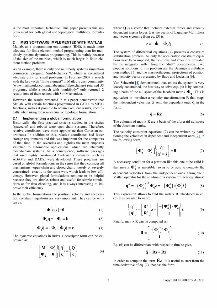
2.1.2 Car example Figure 1 shows the multibody model of a car with 15 degrees of freedom (of which the motion of the steering bar is driven ki-nematically). The front and rear suspensions are of MacPherson and multi-link types, respectively. It has 26 rigid bodies (in-cluding 12 rods) and 225 dependent coordinates (corresponding to 52 points, 19 unit vectors, 7 angles and 5 distances). The tires have been modelled with Pacejka’s magic formula.

Table 1 shows firstly the results of applying the pure Matlab coding. The heaviest steps are the formation of the Jacobian matrix, its LU factorization and the solution of the resulting systems of linear equations with triangular matrices.

Figure 1. Model of a 15 dof car.

All the computer times shown in this paper correspond to 20,000 function evaluations, that is, computations of the deriva-tive of the state vector { }T T T≡y z q previously shown.

The computer used for the calculations has been an Intel Core 2 Extreme processor running at 3 GHz with 4 Gb RAM, and the software releases have been Matlab 2008b and Microsoft Vis-ual Studio 2003.

Table 1. Computer times for a car. Matlab original

inplementation With DLLs Sparse matrices and renumbering

Total 1267,95 s 499,64 s 287,28 s FormFi 262,4 s 2,43 s 2,53 s FormFiq 394,7 s 10.12 s 9,76 s derivR 408,8 s 423,3 s 207,8 s

LU fact. 383,18 371,89 139,64

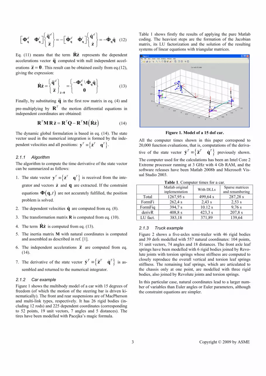
2.1.3 Truck example Figure 2 shows a five-axles semi-trailer with 46 rigid bodies and 39 dofs modelled with 557 natural coordinates: 104 points, 51 unit vectors, 74 angles and 18 distances. The front axle leaf springs have been modelled with 6 rigid bodies joined by Revo-lute joints with torsion springs whose stiffness are computed to closely reproduce the overall vertical and torsion leaf springs stiffness. The remaining leaf springs, which are articulated to the chassis only at one point, are modelled with three rigid bodies, also joined by Revolute joints and torsion springs.

In this particular case, natural coordinates lead to a larger num-ber of variables than Euler angles or Euler parameters, although the constraint equations are simpler.

4 Copyright © 2009 by ASME

Figure 2. Semi-trailer with 5 axles and 35 dofs.

Table 2. Computer times for a semi-trailer. Matlab original

inplementation With DLLs Sparse matrices and renumbering

Total 9731,768 s 948,061 s 717,577 s FormFi 845,783 s 4,017 s 11,509 s FormFiq 7582,293 s 75,723 s 83,086 s derivR 9711,617 s 939,352 s 710,562 s

LU fact. 341,623 s 387,128 s 147,129 s

Table 2 shows the obtained calculation times, which are very big with the pure Matlab implementation. It can be seen that the C/C++ programming of the Jacobian matrix formation divides by 100 the calculation times. The last column shows the im-provements achieved by the variable renumbering and the re-duction of the fill-in in the LU factorization by using sparse matrices. The Jacobian matrix formation times increase because the round errors are bigger and the positions returned by the integrator must be corrected.

It is not easy to obtain large improvements with this global formulation, and it can be proved that this formulation cannot reach a high efficiency.

2.2 Implementing a topological formulation The topological semi-recursive formulation is based on a dou-ble velocity transformation. First the closed-loops are opened and a velocity transformation that maps relative velocities onto Cartesian velocities is introduced symbolically. Then, a second velocity transformation applied numerically on a small system of equations leads to an even smaller system of equations in the independent relative accelerations.

The necessary improvement over global formulation must be to reduce the size of the numerical problems to solve. This can be carried out with semi-recursive and fully recursive formula-tions. Since this paper has educational and practical purposes, a semi-recursive formulation has been chosen to keep it as simple as possible, because it is far simpler than the fully recursive ones.

Open-chain systems, when formulated using relative coordi-nates, avoid constraint equations. If the system has closed loops, relative coordinates are not independent. The usual way to deal with these systems is to open the loops by removing

some joints (and by eliminating the rods, if they exist) and to carry out the dynamic analysis by imposing the corresponding constraint equations.

In the formulation that is described here, the geometry of each moving body is defined in a reference frame attached to the moving body in the input joint by using natural coordinates, i. e., by defining a set of points and unit vectors that describe the geometry of the body and its joints. In this way, the geometry is simpler and clearer than when using multiple “markers” or additional reference frames. When needed, this geometric in-formation is easily transformed to the global reference frame using the body position variables, that are the position vector of the origin of the moving reference frame ir and the transforma-

tion matrix iA .

The Cartesian velocities and accelerations are defined by the vectors,

, i ii i

i i

⎧ ⎫ ⎧ ⎫≡ ≡⎨ ⎬ ⎨ ⎬⎩ ⎭ ⎩ ⎭

s sZ Z

ω ω (15)

where is and is are respectively the velocity and acceleration of the point attached to body i that instantaneously coincides with the origin of the inertial reference frame. In this way, all bodies share the same reference point coordinates, which has important advantages. For instance, the recursive formulas that give the Cartesian velocities and accelerations of body i in terms of those of body 1i − are very simple because they do not need transformation matrices:

1

1

i i i i

i i i i i

z

z−

−

= +

= + +

Z Z b

Z Z b d (16)

Vectors ib and id depend on the joint type (Revolute or

Prismatic) that joins bodies i and 1i − :

( ) ( )1

1

1

2,

2,

i iR R i i i i i ij j

i i i i

i i i iP Pj j

s

ϕ ϕϕ

−

−

−

× ⎧ ⎫+ × ×⎧ ⎫= =⎨ ⎬ ⎨ ⎬

×⎩ ⎭ ⎩ ⎭×⎧ ⎫ ⎧ ⎫

= =⎨ ⎬ ⎨ ⎬⎩ ⎭ ⎩ ⎭

r u ω u r ub d

u ω u

u ω ub d

0 0

(17)

Vectors Z and Z are respectively the vectors that contain the Cartesian velocities and accelerations of all the bodies:

{ }{ }

1 2

1 2

, T T T Tn

T T T Tn

=

=

Z Z Z Z

Z Z Z Z (18)

The virtual power of the inertia and external forces acting on the whole system can be expressed as:

( )1

0n

Ti i i i

i

∗

=

− =∑Z M Z Q (19)

5 Copyright © 2009 by ASME

where

( )1 2

1 2

diag , ,...,

, ,...,

n

T T T Tn

≡

⎡ ⎤= ⎣ ⎦

M M M M

Q Q Q Q (20)

being

i i ii

i i i i i i

i i i i ii

i i i i i i i i i i

m mm m

mm

−⎡ ⎤⎢ ⎥−⎣ ⎦

−⎧ ⎫= ⎨ ⎬− −⎩ ⎭

3I gM =

g J g g

F ωω gQ

g F ω J ω g ω ω g

(21)

respectively the inertia matrix and the vector of external and velocity dependent inertia forces acting on body i with Carte-sian velocities and accelerations (15).

In order to eliminate the dependent virtual velocities i∗Z in eq.

(19) it is possible to introduce a velocity transformation be-tween Cartesian and open-chain relative velocities, in the form:

1 1 2 2 ... n nz z z= + + + =Z R R R Rz (22)

The j-th column of matrix R are the velocities of all the bodies that are upwards of joint j , in which a unit relative velocity is introduced keeping null all the remaining relative velocities.

Assume that the input joint of a body has the same number than this body, and that open-chain bodies and joints have been numbered from the leaves to the root of the spanning tree. At this point it is very useful to introduce the path matrix T that defines the connectivity of the mechanism. Its rows correspond to bodies and its columns to joints. Element ijT is 1 if body i

is upwards of joint j and 0 otherwise. Then matrix T is upper triangular; its column i defines the bodies that are upwards of joint i ; its row j define the joints that are downwards of body j , between the root body and it. Then, expression (22) can be

written in the form:

( )1 2diag , , , N d= ≡R T b b b TR (23)

where ib , according to eq. (16), is the Cartesian velocity of all

bodies upwards of joint i when 1iz = , and 0, jz j i= ≠ .

Remember that vector ib represents the velocity of the point that coincides with the inertial frame origin, that is the same for all bodies.

When expression (23) is used to put Cartesian velocities and accelerations in terms of their relative counterparts, this is ob-tained:

d

d d

= =

= +

Z Rz TR z

Z TR z TR z (24)

By substituting eqs. (24) into eq. (19), multiplying by T TdR T

and taking into account that the relative open-chain virtual velocities are independent, a new set of dynamic equations is obtained:

( ) ( )T T T Td d d d= −R T MT R z R T Q MTR z (25)

This equation corresponds to the open-chain dynamics and can be written more compactly in the form:

oc ext in= +M z Q Q (26)

It is very interesting to consider the effect that the multiplica-tion by the path matrix T has on the matrix and right hand side vector of eqs. (25) or (26). For instance, the element ( ),i j of

matrix ocM is:

( ) oc Tij i i j i jΣ= ≤M b M b (27)

where iΣM is the accumulation or sum of all inertia matrices

defined by (21) and corresponding to bodies that are upwards of body i in the open-chain system.

Similarly the element i of vector ext T Td=Q R T Q can be

expressed as:

ext Ti i i

Σ=Q b Q (28)

where iΣQ represents the accumulation or sum of all forces in

the form of expression (21) that act on the bodies upwards of the element i . The same happens with forces inQ in exp. (26).

The matrix and vector in eqs. (27) and (28) show the advan-tages of numbering the bodies and joints from the leaves to the root: the Gaussian elimination or the LU factorization keeps the pattern of zeros in the matrix, i.e., it maintains the skyline or the sparsity pattern of this matrix, avoiding some arithmetic operations.

The eqs. (31) constitute a system of ordinary differential equa-tions whose coefficient matrix and right-hand side vector can be computed recursively in a very efficient way.

The dynamics of closed-loop multibody systems can be formu-lated by adding the constraint equations to the dynamic equa-tions corresponding to the open-chain system obtained previ-ously. Here the global method described previously can be applied with advantages, because the problem size is much lower with relative coordinates.

An independent subset of relative coordinates is chosen in such a way that a set of ordinary differential equations will be ob-tained again. This is carried out by a new velocity transforma-tion similar to the one introduced by eqs. (24). In this case, the transformation matrix R will be obtained numerically as in the global formulation.

6 Copyright © 2009 by ASME

The closing-loop constraint equations are first formulated in Cartesian coordinates and then transformed to relative coordi-nates. In this paper two ways to set the closed-loop constraint equations will be considered. The first one is the cutting joint method, which is very common in the literature. The second method to open the loops consists of the elimination of the rods (slender bodies with two spherical joints and a negligible mo-ment of inertia around the direction of the axis). This second procedure is very interesting in applications, as the car suspen-sion system considered previously. Reference [2] shows how to take into account rod’s inertia in an exact way, Here only the kinematic constraints for closing the loops will be considered.

The kinematic constraint imposed by a rod is a constant dis-tance condition that can be expressed as:

( ) ( ) 2 0T

j k j k jkl− − − =r r r r (29)

On the other hand, the kinematic constraints corresponding to the removal of a Revolute can be defined with natural coordi-nates as (only eqs. (30) for an Spherical joint):

( ) 3 independent equationsj k− =r r 0 (30)

( ) only 2 independent equationsj k− =u u 0 (31)

The constraint equations (29)-(31) shall be expressed in terms of the relative coordinates z. This is not difficult, because points jr and kr , and unit vectors ju and ku can be ex-pressed as functions of the relative coordinates of the joints in their respective branches of the open-chain system.

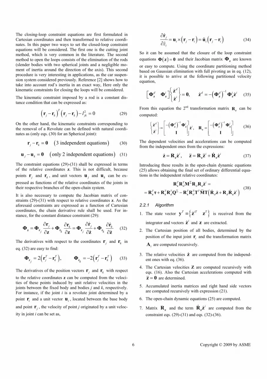
It is also necessary to compute the Jacobian matrix of con-straints (29)-(31) with respect to relative coordinates z. As the aforesaid constraints are expressed as a function of Cartesian coordinates, the chain derivative rule shall be used. For in-stance, for the constant distance constraint (29):

j jk kj k j k

∂ ∂∂ ∂= + = +

∂ ∂ ∂ ∂z r r r r

r rr rΦ Φ Φ Φ Φz z z z

(32)

The derivatives with respect to the coordinates jr and kr in eq. (32) are easy to find:

( ) ( )2 , 2T T T Tj k j kj k

= − = − −r rΦ r r Φ r r (33)

The derivatives of the position vectors jr and kr with respect to the relative coordinates z can be computed from the veloci-ties of these points induced by unit relative velocities in the joints between the fixed body and bodies j and k, respectively. For instance, if the joint i is a revolute joint determined by a point ir and a unit vector iu , located between the base body

and point jr , the velocity of point j originated by a unit veloc-ity in joint i can be set as,

( ) ( )ji j i i j i

iz∂

= × − = −∂

ru r r u r r (34)

So it can be assumed that the closure of the loop constraint equations ( ) =Φ z 0 and their Jacobian matrix zΦ are known or easy to compute. Using the coordinate partitioning method based on Gaussian elimination with full pivoting as in eq. (12), it is possible to arrive at the following partitioned velocity equation,

( ) 1,

dd i d d i i

i

−⎧ ⎫⎡ ⎤ = = −⎨ ⎬⎣ ⎦

⎩ ⎭z z z z

zΦ Φ 0 z Φ Φ z

z (35)

From this equation the 2nd transformation matrix zR can be computed:

( ) ( )1 1

, d d i d i

ii

− −⎡ ⎤ ⎡ ⎤⎧ ⎫ − −⎢ ⎥ ⎢ ⎥= =⎨ ⎬⎢ ⎥ ⎢ ⎥⎩ ⎭ ⎣ ⎦ ⎣ ⎦

z z z zz

z Φ Φ Φ Φz Rz I I

(36)

The dependent velocities and accelerations can be computed from the independent ones from the expressions:

, i i i= = +z z zz R z z R z R z (37)

Introducing these results in the open-chain dynamic equations (25) allows obtaining the final set of ordinary differential equa-tions in the independent relative coordinates:

( )

T T id d

T T T T T T id d d d

∑

∑

=

= + − +z z

z z z z

R R M R R z

R τ R R Q R R T MT R z R R z (38)

2.2.1 Algorithm

1. The state vector { }T iT T≡y z z is received from the

integrator and vectors iz and z are extracted.

2. The Cartesian position of all bodies, determined by the position of the input joint ir and the transformation matrix

iA are computed recursively.

3. The relative velocities z are computed from the independ-ent ones with eq. (36).

4. The Cartesian velocities Z are computed recursively with eqs. (16). Also the Cartesian accelerations computed with =z 0 are determined.

5. Accumulated inertia matrices and right hand side vectors are computed recursively with expression (21).

6. The open-chain dynamic equations (25) are computed.

7. Matrix zR and the term izR z are computed from the

constraint eqs. (29)-(31) and eqs. (32)-(36).

7 Copyright © 2009 by ASME

8. The dynamic equations (38) are evaluated and the inde-pendent accelerations iz are computed.

9. The derivative of the state vector is formed and returned to the integrator.

2.2.2 Car example The same car shown in Figure 1 is simulated with the described semi-recursive formulation. In this case all the joints have to be Revolute or Prismatic, and this makes necessary to include auxiliary elements without mass (with a point and two orthogo-nal unit vectors) in the joints with more than one dof and be-tween the fixed element and the chassis or other floating ele-ments (with 6 dofs respect to the fixed element).

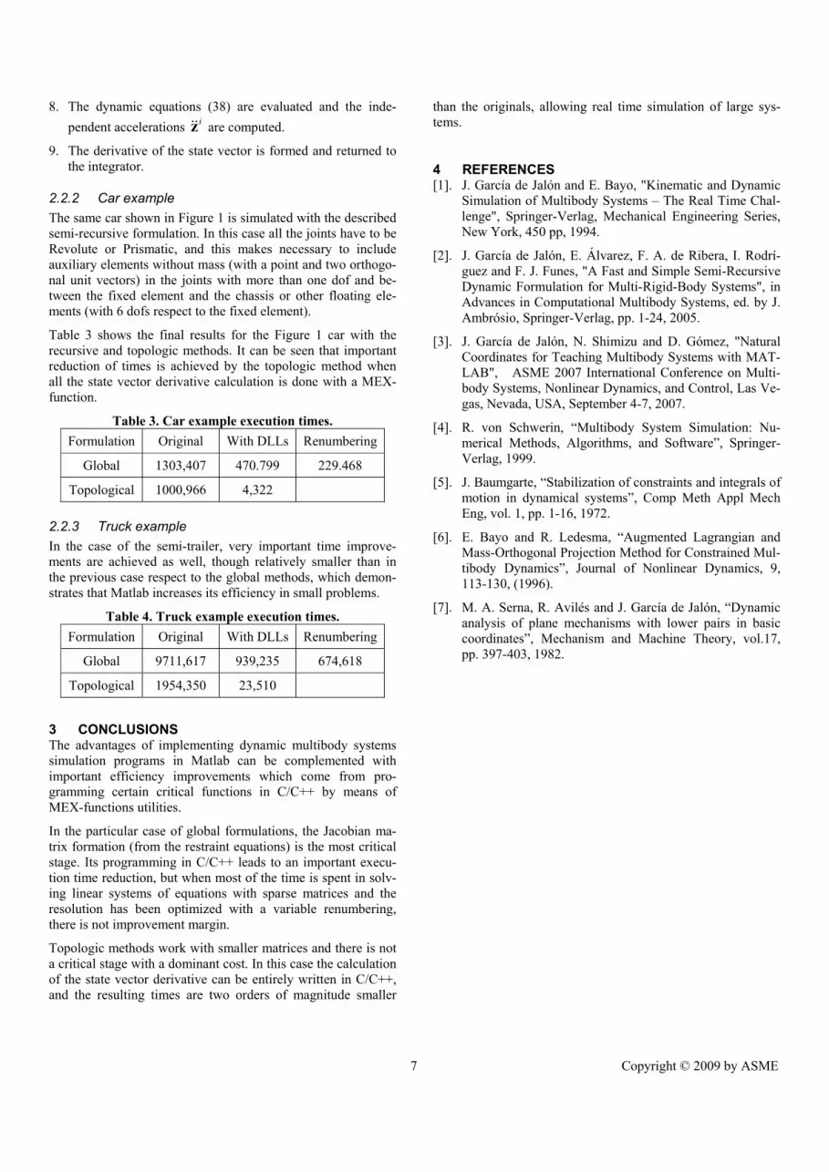
Table 3 shows the final results for the Figure 1 car with the recursive and topologic methods. It can be seen that important reduction of times is achieved by the topologic method when all the state vector derivative calculation is done with a MEX-function.

Table 3. Car example execution times. Formulation Original With DLLs Renumbering

Global 1303,407 470.799 229.468

Topological 1000,966 4,322

2.2.3 Truck example In the case of the semi-trailer, very important time improve-ments are achieved as well, though relatively smaller than in the previous case respect to the global methods, which demon-strates that Matlab increases its efficiency in small problems.

Table 4. Truck example execution times. Formulation Original With DLLs Renumbering

Global 9711,617 939,235 674,618

Topological 1954,350 23,510

3 CONCLUSIONS The advantages of implementing dynamic multibody systems simulation programs in Matlab can be complemented with important efficiency improvements which come from pro-gramming certain critical functions in C/C++ by means of MEX-functions utilities.

In the particular case of global formulations, the Jacobian ma-trix formation (from the restraint equations) is the most critical stage. Its programming in C/C++ leads to an important execu-tion time reduction, but when most of the time is spent in solv-ing linear systems of equations with sparse matrices and the resolution has been optimized with a variable renumbering, there is not improvement margin.

Topologic methods work with smaller matrices and there is not a critical stage with a dominant cost. In this case the calculation of the state vector derivative can be entirely written in C/C++, and the resulting times are two orders of magnitude smaller

than the originals, allowing real time simulation of large sys-tems.

4 REFERENCES [1]. J. García de Jalón and E. Bayo, "Kinematic and Dynamic

Simulation of Multibody Systems – The Real Time Chal-lenge", Springer-Verlag, Mechanical Engineering Series, New York, 450 pp, 1994.

[2]. J. García de Jalón, E. Álvarez, F. A. de Ribera, I. Rodrí-guez and F. J. Funes, "A Fast and Simple Semi-Recursive Dynamic Formulation for Multi-Rigid-Body Systems", in Advances in Computational Multibody Systems, ed. by J. Ambrósio, Springer-Verlag, pp. 1-24, 2005.

[3]. J. García de Jalón, N. Shimizu and D. Gómez, "Natural Coordinates for Teaching Multibody Systems with MAT-LAB", ASME 2007 International Conference on Multi-body Systems, Nonlinear Dynamics, and Control, Las Ve-gas, Nevada, USA, September 4-7, 2007.

[4]. R. von Schwerin, “Multibody System Simulation: Nu-merical Methods, Algorithms, and Software”, Springer-Verlag, 1999.

[5]. J. Baumgarte, “Stabilization of constraints and integrals of motion in dynamical systems”, Comp Meth Appl Mech Eng, vol. 1, pp. 1-16, 1972.

[6]. E. Bayo and R. Ledesma, “Augmented Lagrangian and Mass-Orthogonal Projection Method for Constrained Mul-tibody Dynamics”, Journal of Nonlinear Dynamics, 9, 113-130, (1996).

[7]. M. A. Serna, R. Avilés and J. García de Jalón, “Dynamic analysis of plane mechanisms with lower pairs in basic coordinates”, Mechanism and Machine Theory, vol.17, pp. 397-403, 1982.