Embed Size (px)
Citation preview
4 Programming In MatlabIn this chapter, we study the fundamentals of programming in Matlab. We beginwith a study of logical arrays and the operators and method that make them soeffective in Matlab programming.
Table of Contents4.1 Logical Arrays . . . . . . . . . . . . . . . . . . . . . . . . . . . . . . . . . . . . . . . . . . . . . . 261
Relational Operators 263How Logical Arrays are Used 265Logical Operators 277Exercises 285Answers 289
4.2 Control Structures in Matlab . . . . . . . . . . . . . . . . . . . . . . . . . . . . . . . . . 299If 299Else 300Elseif 301Switch, Case, and Otherwise 304Loops 306For k = A 311Break and Continue 312Any and All 314Nested Loops 316Fourier Series — An Application of a For Loop 318Exercises 323Answers 327
4.3 Functions in Matlab . . . . . . . . . . . . . . . . . . . . . . . . . . . . . . . . . . . . . . . . . 333Anonymous Functions 333Function M-Files 338More Than One Output 343No Output 346Exercises 349Answers 353
4.4 Variable Scope in Matlab . . . . . . . . . . . . . . . . . . . . . . . . . . . . . . . . . . . . 361The Base Workspace 361Scripts and the Base Workspace 362Function Workspaces 364Global Variables 368Persistent Variables 369Exercises 372Answers 377
260 Chapter 4 Programming In Matlab
4.5 Subfunctions in Matlab . . . . . . . . . . . . . . . . . . . . . . . . . . . . . . . . . . . . . . 379Calling Functions From Script Files 380Subfunctions 383Adding Functionality to our Program 385Completing rationalArithmetic.m 391Exercises 393
4.6 Nested Functions in Matlab . . . . . . . . . . . . . . . . . . . . . . . . . . . . . . . . . . 399Variable Scope in Nested Functions 400Graphical User Interfaces 403Button Groups and Radio Buttons 406Adding a Function Callback to the UIButtonGroup 409Popup Menus 411Edit Boxes 415Appendix 418Exercises 422Answers 430
Copyright
All parts of this Matlab Programming textbook are copyrighted in the nameof Department of Mathematics, College of the Redwoods. They are not inthe public domain. However, they are being made available free for usein educational institutions. This offer does not extend to any applicationthat is made for profit. Users who have such applications in mind shouldcontact David Arnold at [email protected] or Bruce Wagner [email protected].
This work (including all text, Portable Document Format files, and any otheroriginal works), except where otherwise noted, is licensed under a CreativeCommons Attribution-NonCommercial-ShareAlike 2.5 License, and is copy-righted C©2006, Department of Mathematics, College of the Redwoods. Toview a copy of this license, visit http://creativecommons.org/licenses/by-nc-sa/2.5/ or send a letter to Creative Commons, 543 Howard Street, 5th Floor,San Francisco, California, 94105, USA.
Section 4.1 Logical Arrays 261
4.1 Logical ArraysWe begin this section by demonstraing how Matlab determines the truth or
falsehood of a statement. Enter the following array at the Matlab prompt.
>> x=[true false]x =
1 0
Note that that true evaluates to 1, while false evaluates to zero. Moreover, thearray stored in the variable x in an entirely new type of datatype, called a logicalarray.
>> whosName Size Bytes Class
x 1x2 2 logical array
Note that each entry in the logical vector x takes one byte of storage. Note thatthis logical type is a completely new datatype. Indeed, it is instructive to comparethe vector x with the following vector y
>> y=[1 0]y =
1 0
On the surface, it appears that the variables x and y contain exactly the samedata, that is until one checks the datatypes with Matlab’s whos command.
>> whosName Size Bytes Class
x 1x2 2 logical arrayy 1x2 16 double array
Copyrighted material. See: http://msenux.redwoods.edu/Math4Textbook/1
262 Chapter 4 Programming in Matlab
Note that vector y is of class double, using 8 bytes to store each entry.Alternatively, we can check the class with Matlab’s class command. On the
one hand, the command
>> class(x)ans =logical
informs us that vector x has class logical. On the other hand, the command
>> class(y)ans =double
informs us that the vector y has class double.Like some of the other conversion operators we’ve seen (like uint8), Matlab
provides an operator that will convert numeric arrays to logical arrays. Anynonzero real number is converted to a logical 1 (true) and zeros are converted tological 0 (false).
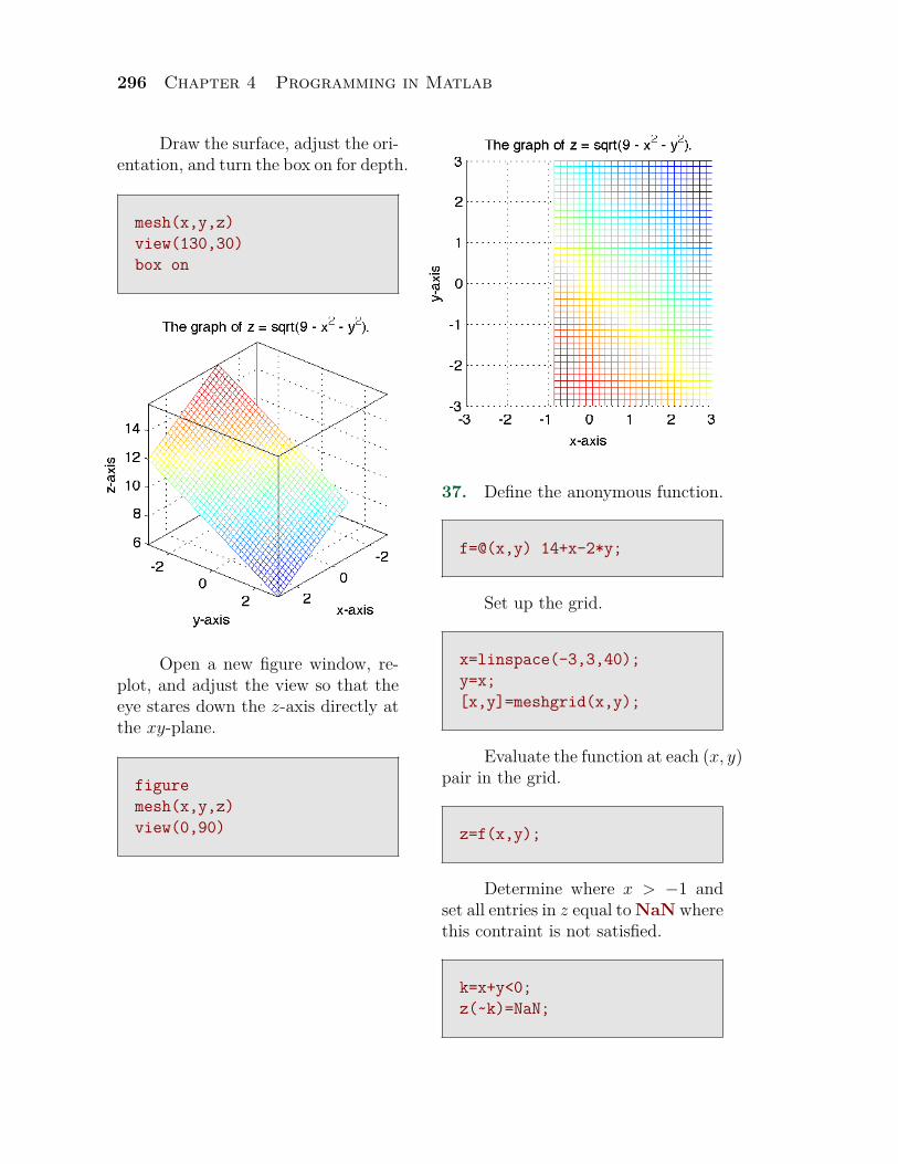
To see this in action, first enter the following matrix A.
>> A=[0 1 3;4 0 0; 5 7 -11]A =
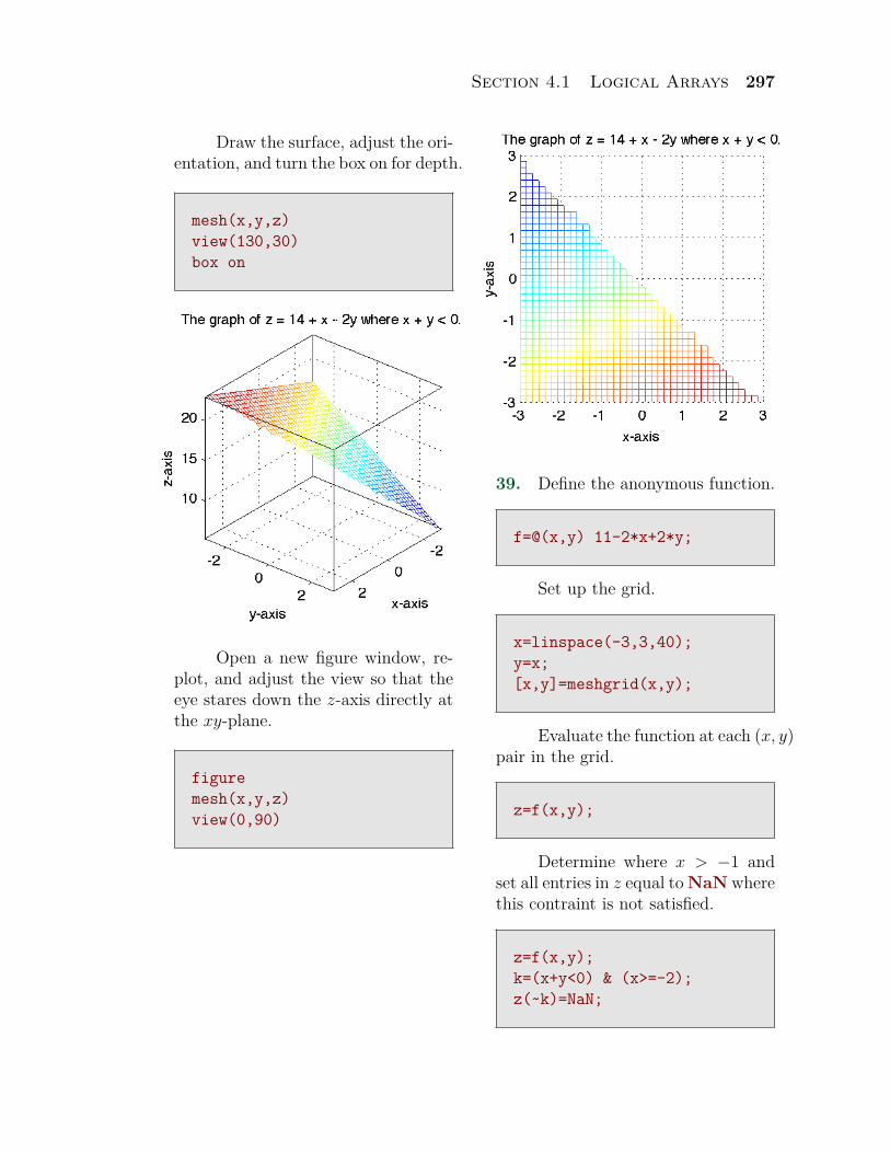
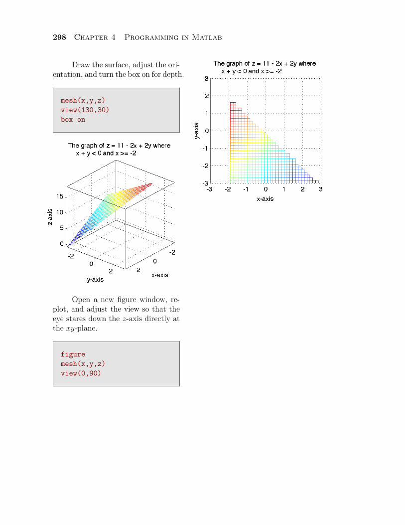
0 1 34 0 05 7 -11
Note that A has class double.
>> class(A)ans =double
Now, convert A to a logical array.
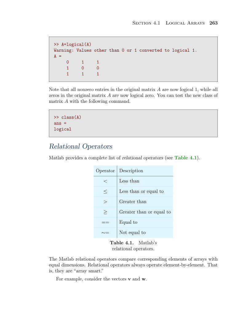
Section 4.1 Logical Arrays 263
>> A=logical(A)Warning: Values other than 0 or 1 converted to logical 1.A =
0 1 11 0 01 1 1
Note that all nonzero entries in the original matrix A are now logical 1, while allzeros in the original matrix A are now logical zero. You can test the new class ofmatrix A with the following command.
>> class(A)ans =logical
Relational OperatorsMatlab provides a complete list of relational operators (see Table 4.1).
Operator Description
< Less than
≤ Less than or equal to
> Greater than
≥ Greater than or equal to
== Equal to
∼= Not equal to
Table 4.1. Matlab’srelational operators.
The Matlab relational operators compare corresponding elements of arrays withequal dimensions. Relational operators always operate element-by-element. Thatis, they are “array smart.”
For example, consider the vectors v and w.
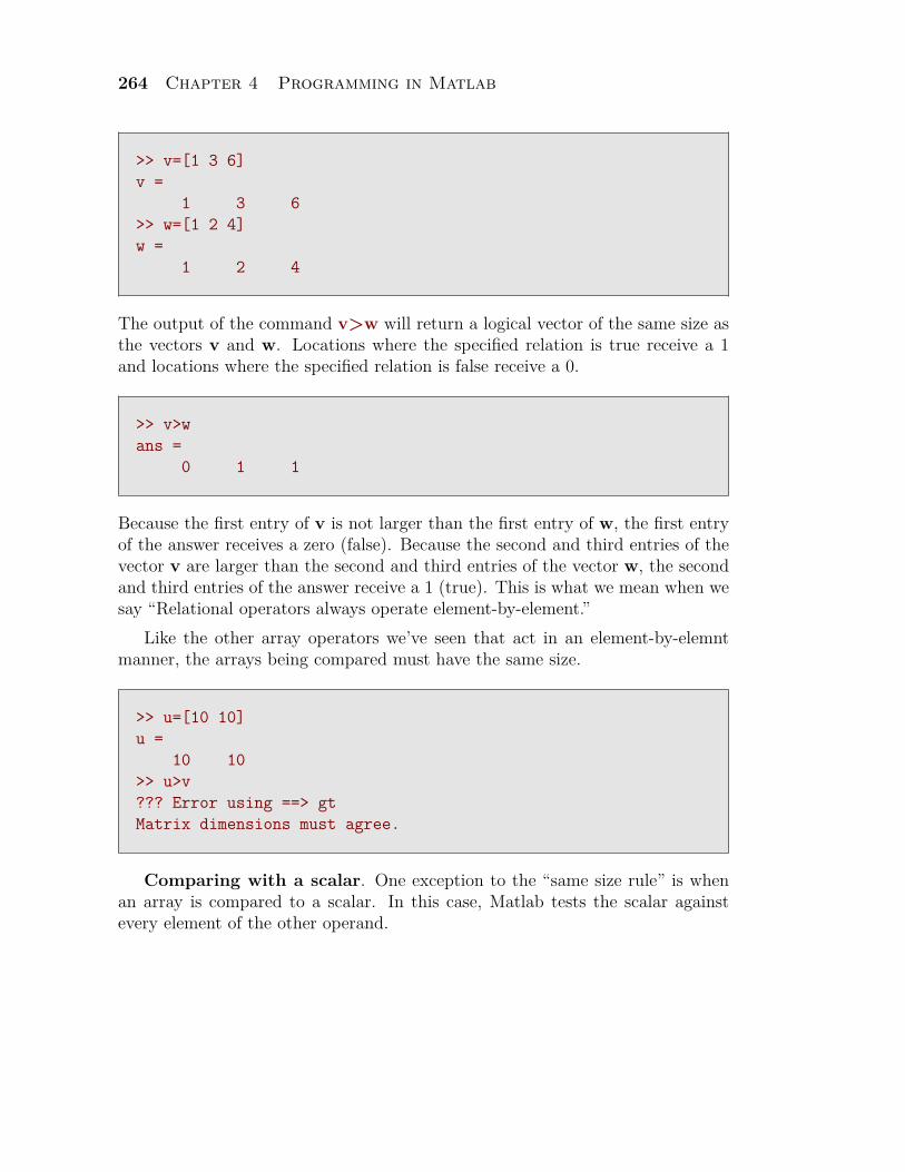
264 Chapter 4 Programming in Matlab
>> v=[1 3 6]v =
1 3 6>> w=[1 2 4]w =
1 2 4
The output of the command v>w will return a logical vector of the same size asthe vectors v and w. Locations where the specified relation is true receive a 1and locations where the specified relation is false receive a 0.
>> v>wans =
0 1 1
Because the first entry of v is not larger than the first entry of w, the first entryof the answer receives a zero (false). Because the second and third entries of thevector v are larger than the second and third entries of the vector w, the secondand third entries of the answer receive a 1 (true). This is what we mean when wesay “Relational operators always operate element-by-element.”
Like the other array operators we’ve seen that act in an element-by-elemntmanner, the arrays being compared must have the same size.
>> u=[10 10]u =
10 10>> u>v??? Error using ==> gtMatrix dimensions must agree.
Comparing with a scalar. One exception to the “same size rule” is whenan array is compared to a scalar. In this case, Matlab tests the scalar againstevery element of the other operand.
Section 4.1 Logical Arrays 265
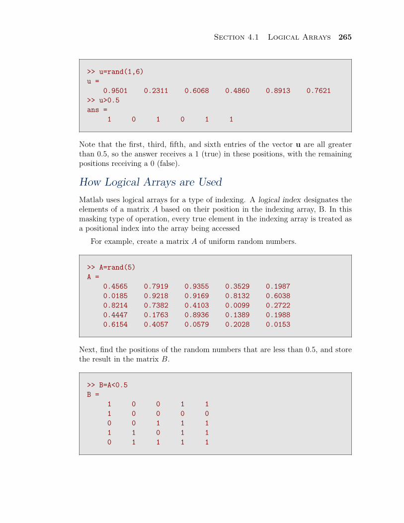
>> u=rand(1,6)u =
0.9501 0.2311 0.6068 0.4860 0.8913 0.7621>> u>0.5ans =
1 0 1 0 1 1
Note that the first, third, fifth, and sixth entries of the vector u are all greaterthan 0.5, so the answer receives a 1 (true) in these positions, with the remainingpositions receiving a 0 (false).
How Logical Arrays are UsedMatlab uses logical arrays for a type of indexing. A logical index designates theelements of a matrix A based on their position in the indexing array, B. In thismasking type of operation, every true element in the indexing array is treated asa positional index into the array being accessed
For example, create a matrix A of uniform random numbers.
>> A=rand(5)A =
0.4565 0.7919 0.9355 0.3529 0.19870.0185 0.9218 0.9169 0.8132 0.60380.8214 0.7382 0.4103 0.0099 0.27220.4447 0.1763 0.8936 0.1389 0.19880.6154 0.4057 0.0579 0.2028 0.0153
Next, find the positions of the random numbers that are less than 0.5, and storethe result in the matrix B.
>> B=A<0.5B =
1 0 0 1 11 0 0 0 00 0 1 1 11 1 0 1 10 1 1 1 1
266 Chapter 4 Programming in Matlab
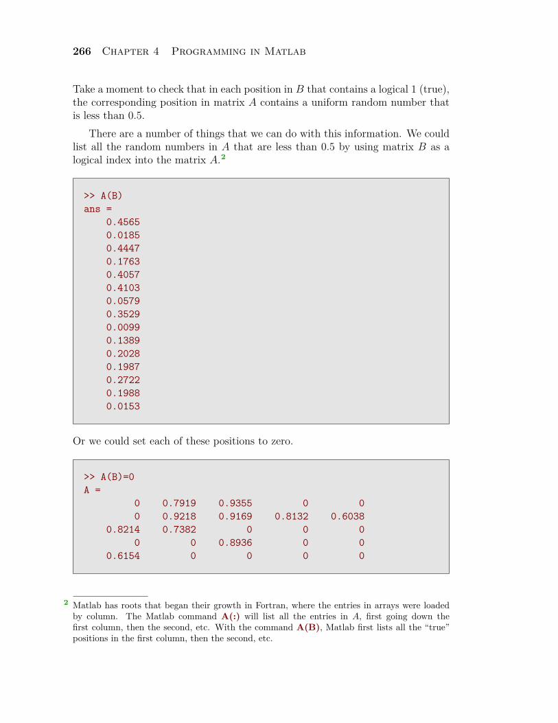
Take a moment to check that in each position in B that contains a logical 1 (true),the corresponding position in matrix A contains a uniform random number thatis less than 0.5.
There are a number of things that we can do with this information. We couldlist all the random numbers in A that are less than 0.5 by using matrix B as alogical index into the matrix A.2
>> A(B)ans =
0.45650.01850.44470.17630.40570.41030.05790.35290.00990.13890.20280.19870.27220.19880.0153
Or we could set each of these positions to zero.
>> A(B)=0A =
0 0.7919 0.9355 0 00 0.9218 0.9169 0.8132 0.6038
0.8214 0.7382 0 0 00 0 0.8936 0 0
0.6154 0 0 0 0
Matlab has roots that began their growth in Fortran, where the entries in arrays were loaded2
by column. The Matlab command A(:) will list all the entries in A, first going down thefirst column, then the second, etc. With the command A(B), Matlab first lists all the “true”positions in the first column, then the second, etc.
Section 4.1 Logical Arrays 267
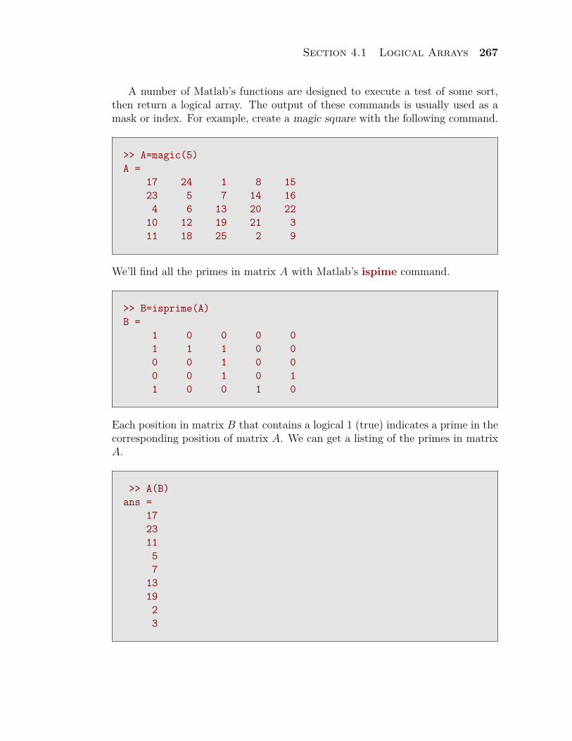
A number of Matlab’s functions are designed to execute a test of some sort,then return a logical array. The output of these commands is usually used as amask or index. For example, create a magic square with the following command.
>> A=magic(5)A =
17 24 1 8 1523 5 7 14 164 6 13 20 22
10 12 19 21 311 18 25 2 9
We’ll find all the primes in matrix A with Matlab’s ispime command.
>> B=isprime(A)B =
1 0 0 0 01 1 1 0 00 0 1 0 00 0 1 0 11 0 0 1 0
Each position in matrix B that contains a logical 1 (true) indicates a prime in thecorresponding position of matrix A. We can get a listing of the primes in matrixA.
>> A(B)ans =
17231157
131923
268 Chapter 4 Programming in Matlab
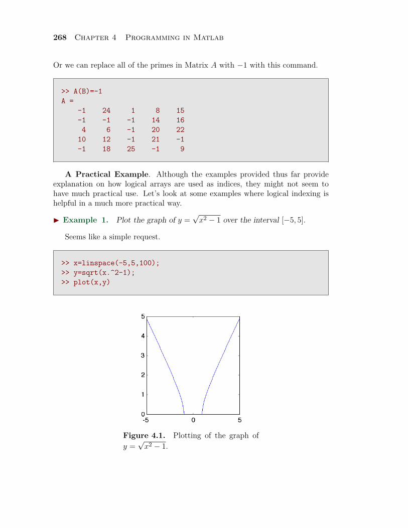
Or we can replace all of the primes in Matrix A with −1 with this command.
>> A(B)=-1A =
-1 24 1 8 15-1 -1 -1 14 164 6 -1 20 22
10 12 -1 21 -1-1 18 25 -1 9
A Practical Example. Although the examples provided thus far provideexplanation on how logical arrays are used as indices, they might not seem tohave much practical use. Let’s look at some examples where logical indexing ishelpful in a much more practical way.
I Example 1. Plot the graph of y =√
x2 − 1 over the interval [−5, 5].
Seems like a simple request.
>> x=linspace(-5,5,100);>> y=sqrt(x.^2-1);>> plot(x,y)
Figure 4.1. Plotting of the graph ofy =
√x2 − 1.
Section 4.1 Logical Arrays 269
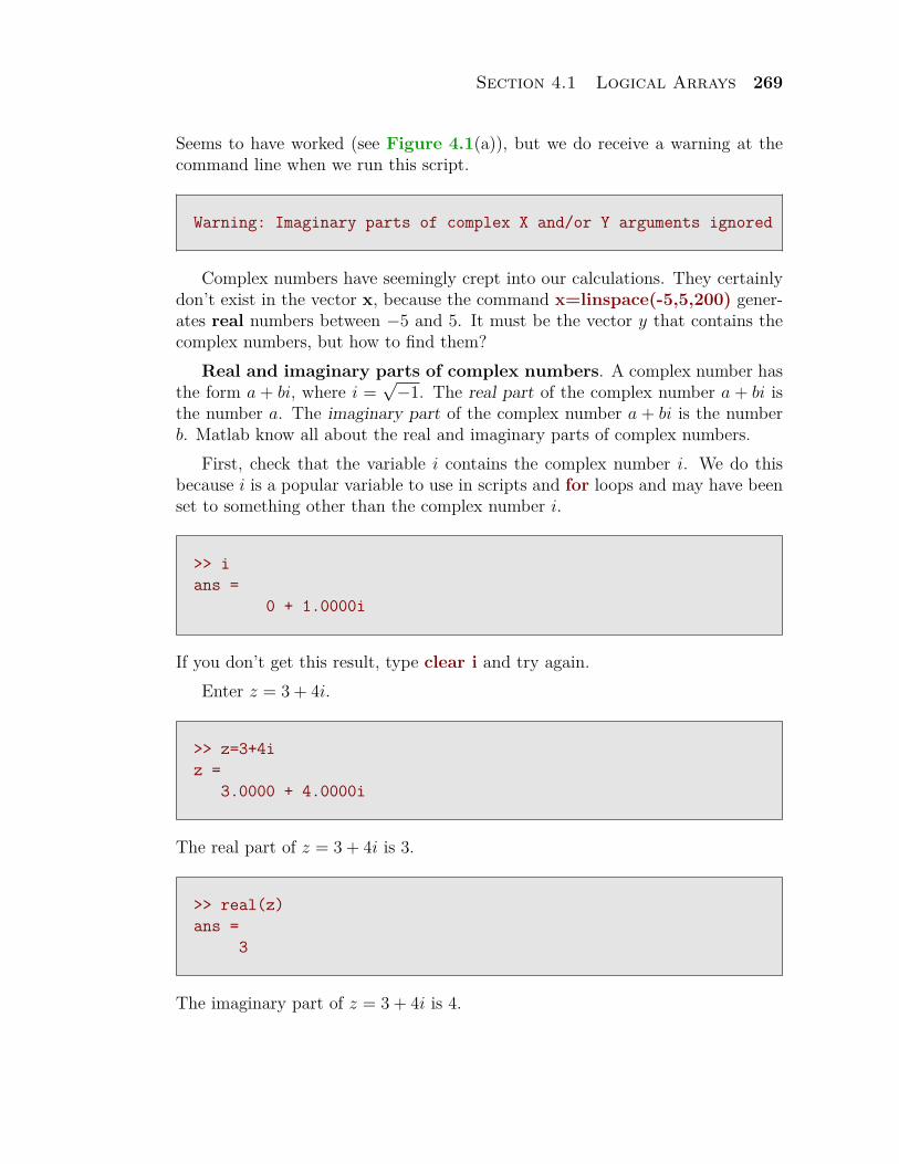
Seems to have worked (see Figure 4.1(a)), but we do receive a warning at thecommand line when we run this script.
Warning: Imaginary parts of complex X and/or Y arguments ignored
Complex numbers have seemingly crept into our calculations. They certainlydon’t exist in the vector x, because the command x=linspace(-5,5,200) gener-ates real numbers between −5 and 5. It must be the vector y that contains thecomplex numbers, but how to find them?
Real and imaginary parts of complex numbers. A complex number hasthe form a + bi, where i =
√−1. The real part of the complex number a + bi is
the number a. The imaginary part of the complex number a + bi is the numberb. Matlab know all about the real and imaginary parts of complex numbers.
First, check that the variable i contains the complex number i. We do thisbecause i is a popular variable to use in scripts and for loops and may have beenset to something other than the complex number i.
>> ians =
0 + 1.0000i
If you don’t get this result, type clear i and try again.Enter z = 3 + 4i.
>> z=3+4iz =
3.0000 + 4.0000i
The real part of z = 3 + 4i is 3.
>> real(z)ans =
3
The imaginary part of z = 3 + 4i is 4.
270 Chapter 4 Programming in Matlab
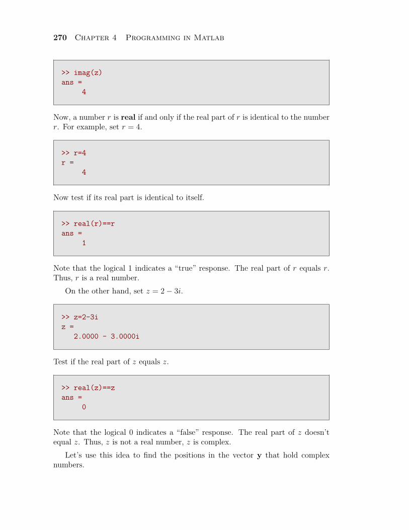
>> imag(z)ans =
4
Now, a number r is real if and only if the real part of r is identical to the numberr. For example, set r = 4.
>> r=4r =
4
Now test if its real part is identical to itself.
>> real(r)==rans =
1
Note that the logical 1 indicates a “true” response. The real part of r equals r.Thus, r is a real number.
On the other hand, set z = 2− 3i.
>> z=2-3iz =
2.0000 - 3.0000i
Test if the real part of z equals z.
>> real(z)==zans =
0
Note that the logical 0 indicates a “false” response. The real part of z doesn’tequal z. Thus, z is not a real number, z is complex.
Let’s use this idea to find the positions in the vector y that hold complexnumbers.
Section 4.1 Logical Arrays 271
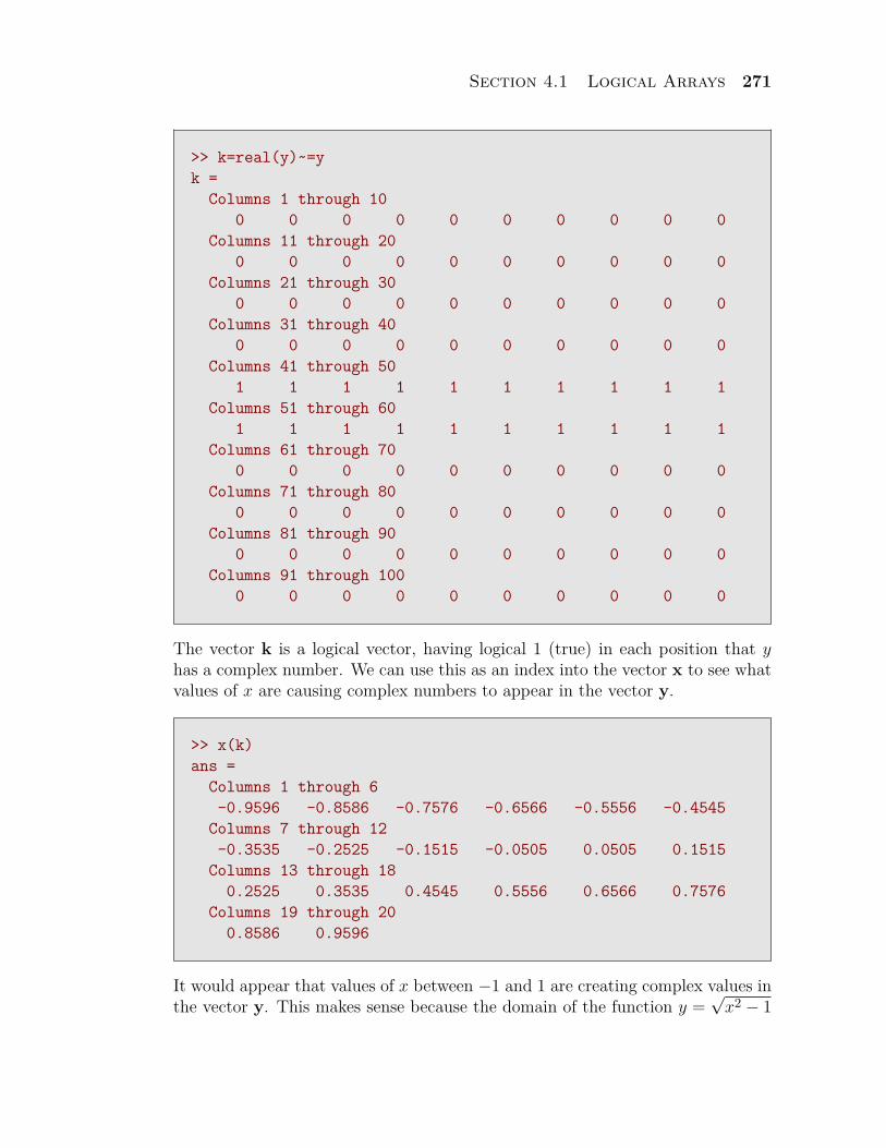
>> k=real(y)~=yk =
Columns 1 through 100 0 0 0 0 0 0 0 0 0
Columns 11 through 200 0 0 0 0 0 0 0 0 0
Columns 21 through 300 0 0 0 0 0 0 0 0 0
Columns 31 through 400 0 0 0 0 0 0 0 0 0
Columns 41 through 501 1 1 1 1 1 1 1 1 1
Columns 51 through 601 1 1 1 1 1 1 1 1 1
Columns 61 through 700 0 0 0 0 0 0 0 0 0
Columns 71 through 800 0 0 0 0 0 0 0 0 0
Columns 81 through 900 0 0 0 0 0 0 0 0 0
Columns 91 through 1000 0 0 0 0 0 0 0 0 0
The vector k is a logical vector, having logical 1 (true) in each position that yhas a complex number. We can use this as an index into the vector x to see whatvalues of x are causing complex numbers to appear in the vector y.
>> x(k)ans =
Columns 1 through 6-0.9596 -0.8586 -0.7576 -0.6566 -0.5556 -0.4545
Columns 7 through 12-0.3535 -0.2525 -0.1515 -0.0505 0.0505 0.1515
Columns 13 through 180.2525 0.3535 0.4545 0.5556 0.6566 0.7576
Columns 19 through 200.8586 0.9596
It would appear that values of x between −1 and 1 are creating complex values inthe vector y. This makes sense because the domain of the function y =
√x2 − 1
272 Chapter 4 Programming in Matlab
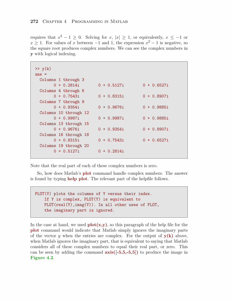
requires that x2 − 1 ≥ 0. Solving for x, |x| ≥ 1, or equivalently, x ≤ −1 orx ≥ 1. For values of x between −1 and 1, the expression x2 − 1 is negative, sothe square root produces complex numbers. We can see the complex numbers iny with logical indexing.
>> y(k)ans =
Columns 1 through 30 + 0.2814i 0 + 0.5127i 0 + 0.6527i
Columns 4 through 60 + 0.7543i 0 + 0.8315i 0 + 0.8907i
Columns 7 through 90 + 0.9354i 0 + 0.9676i 0 + 0.9885i
Columns 10 through 120 + 0.9987i 0 + 0.9987i 0 + 0.9885i
Columns 13 through 150 + 0.9676i 0 + 0.9354i 0 + 0.8907i
Columns 16 through 180 + 0.8315i 0 + 0.7543i 0 + 0.6527i
Columns 19 through 200 + 0.5127i 0 + 0.2814i
Note that the real part of each of these complex numbers is zero.So, how does Matlab’s plot command handle complex numbers. The answer
is found by typing help plot. The relevant part of the helpfile follows.
PLOT(Y) plots the columns of Y versus their index.If Y is complex, PLOT(Y) is equivalent toPLOT(real(Y),imag(Y)). In all other uses of PLOT,the imaginary part is ignored.
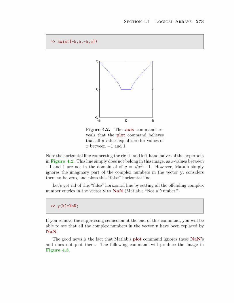
In the case at hand, we used plot(x,y), so this paragraph of the help file for theplot command would indicate that Matlab simply ignores the imaginary partsof the vector y when the entries are complex. For the output of y(k) above,when Matlab ignores the imaginary part, that is equivalent to saying that Matlabconsiders all of these complex numbers to equal their real part, or zero. Thiscan be seen by adding the command axis([-5,5,-5,5]) to produce the image inFigure 4.2.
Section 4.1 Logical Arrays 273
>> axis([-5,5,-5,5])
Figure 4.2. The axis command re-veals that the plot command believesthat all y-values equal zero for values ofx between −1 and 1.
Note the horizontal line connecting the right- and left-hand halves of the hyperbolain Figure 4.2. This line simply does not belong in this image, as x-values between−1 and 1 are not in the domain of of y =
√x2 − 1. However, Matalb simply
ignores the imaginary part of the complex numbers in the vector y, considersthem to be zero, and plots this “false” horizontal line.
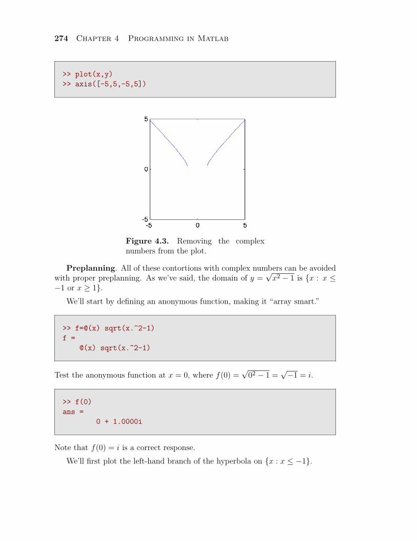
Let’s get rid of this “false” horizontal line by setting all the offending complexnumber entries in the vector y to NaN (Matlab’s “Not a Number.”)
>> y(k)=NaN;
If you remove the suppressing semicolon at the end of this command, you will beable to see that all the complex numbers in the vector y have been replaced byNaN.
The good news is the fact that Matlab’s plot command ignores these NaN’sand does not plot them. The following command will produce the image inFigure 4.3.
274 Chapter 4 Programming in Matlab
>> plot(x,y)>> axis([-5,5,-5,5])
Figure 4.3. Removing the complexnumbers from the plot.
Preplanning. All of these contortions with complex numbers can be avoidedwith proper preplanning. As we’ve said, the domain of y =
√x2 − 1 is {x : x ≤
−1 or x ≥ 1}.We’ll start by defining an anonymous function, making it “array smart.”
>> f=@(x) sqrt(x.^2-1)f =
@(x) sqrt(x.^2-1)
Test the anonymous function at x = 0, where f(0) =√
02 − 1 =√−1 = i.
>> f(0)ans =
0 + 1.0000i
Note that f(0) = i is a correct response.We’ll first plot the left-hand branch of the hyperbola on {x : x ≤ −1}.
Section 4.1 Logical Arrays 275
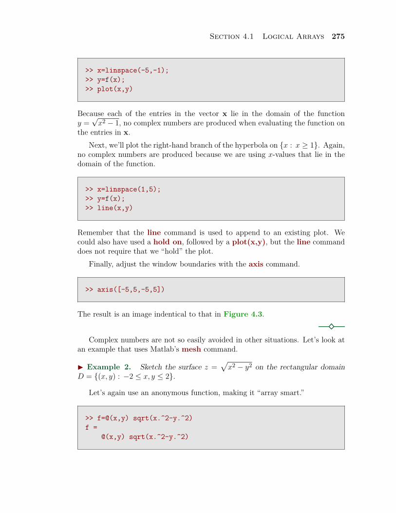
>> x=linspace(-5,-1);>> y=f(x);>> plot(x,y)
Because each of the entries in the vector x lie in the domain of the functiony =
√x2 − 1, no complex numbers are produced when evaluating the function on
the entries in x.Next, we’ll plot the right-hand branch of the hyperbola on {x : x ≥ 1}. Again,
no complex numbers are produced because we are using x-values that lie in thedomain of the function.
>> x=linspace(1,5);>> y=f(x);>> line(x,y)
Remember that the line command is used to append to an existing plot. Wecould also have used a hold on, followed by a plot(x,y), but the line commanddoes not require that we “hold” the plot.
Finally, adjust the window boundaries with the axis command.
>> axis([-5,5,-5,5])
The result is an image indentical to that in Figure 4.3.
Complex numbers are not so easily avoided in other situations. Let’s look atan example that uses Matlab’s mesh command.
I Example 2. Sketch the surface z =√
x2 − y2 on the rectangular domainD = {(x, y) : −2 ≤ x, y ≤ 2}.
Let’s again use an anonymous function, making it “array smart.”
>> f=@(x,y) sqrt(x.^2-y.^2)f =
@(x,y) sqrt(x.^2-y.^2)
276 Chapter 4 Programming in Matlab
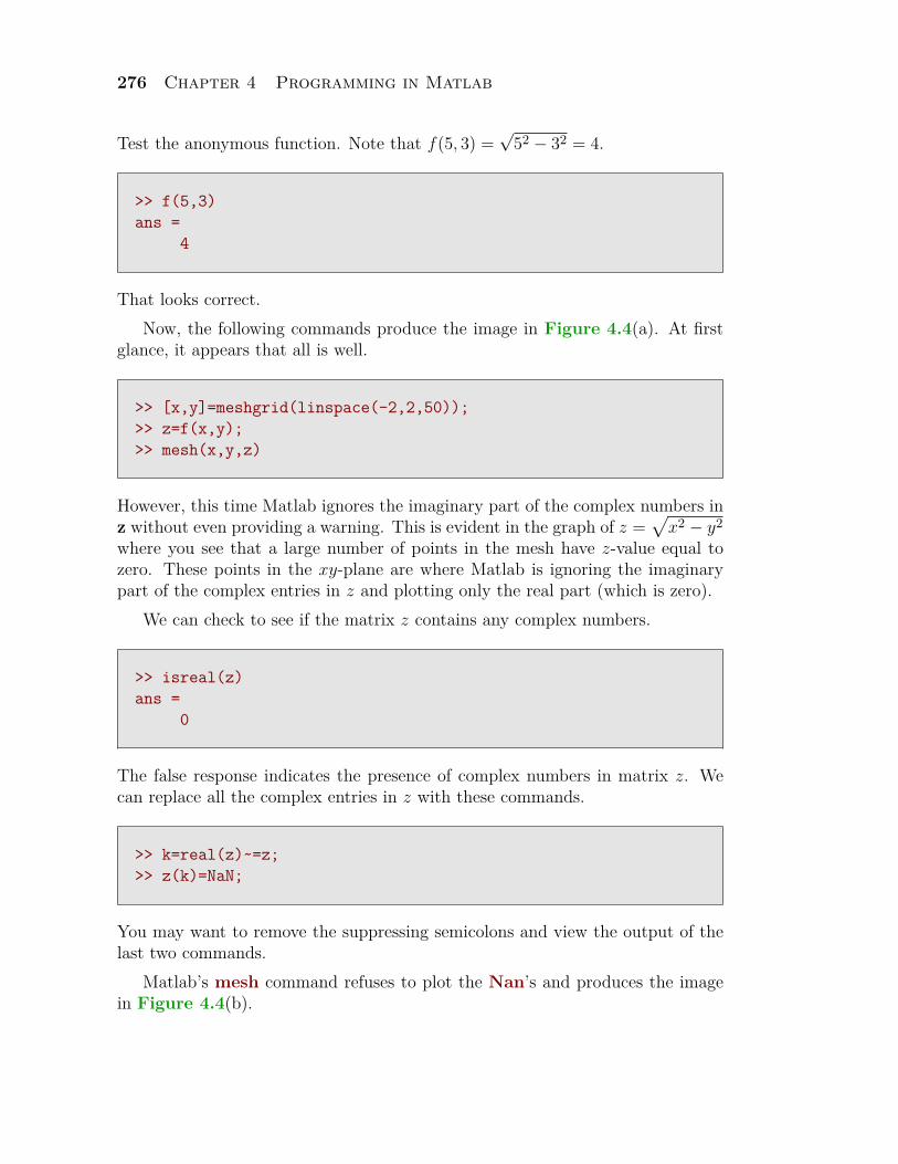
Test the anonymous function. Note that f(5, 3) =√
52 − 32 = 4.
>> f(5,3)ans =
4
That looks correct.Now, the following commands produce the image in Figure 4.4(a). At first
glance, it appears that all is well.
>> [x,y]=meshgrid(linspace(-2,2,50));>> z=f(x,y);>> mesh(x,y,z)
However, this time Matlab ignores the imaginary part of the complex numbers inz without even providing a warning. This is evident in the graph of z =
√x2 − y2
where you see that a large number of points in the mesh have z-value equal tozero. These points in the xy-plane are where Matlab is ignoring the imaginarypart of the complex entries in z and plotting only the real part (which is zero).
We can check to see if the matrix z contains any complex numbers.
>> isreal(z)ans =
0
The false response indicates the presence of complex numbers in matrix z. Wecan replace all the complex entries in z with these commands.
>> k=real(z)~=z;>> z(k)=NaN;
You may want to remove the suppressing semicolons and view the output of thelast two commands.
Matlab’s mesh command refuses to plot the Nan’s and produces the imagein Figure 4.4(b).
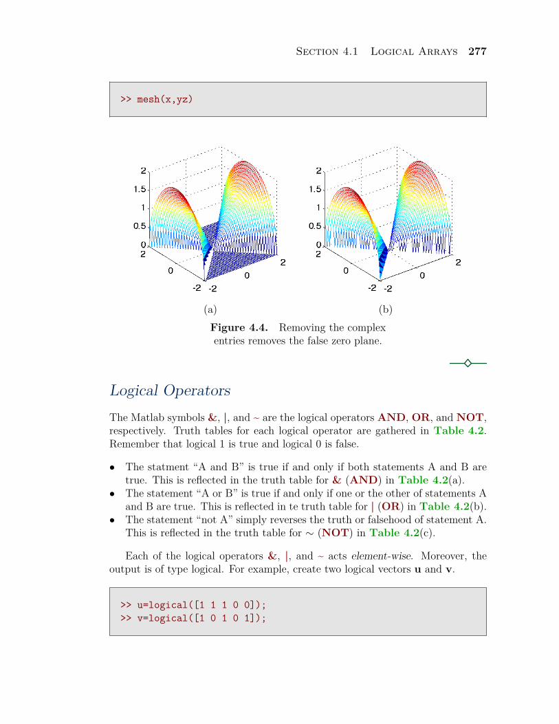
Section 4.1 Logical Arrays 277
>> mesh(x,yz)
(a) (b)Figure 4.4. Removing the complexentries removes the false zero plane.
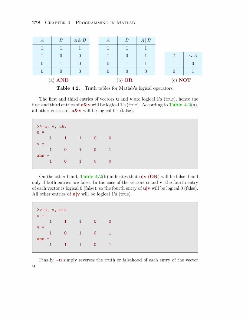
Logical OperatorsThe Matlab symbols &, |, and ~ are the logical operators AND, OR, and NOT,respectively. Truth tables for each logical operator are gathered in Table 4.2.Remember that logical 1 is true and logical 0 is false.
• The statment “A and B” is true if and only if both statements A and B aretrue. This is reflected in the truth table for & (AND) in Table 4.2(a).
• The statement “A or B” is true if and only if one or the other of statements Aand B are true. This is reflected in te truth table for | (OR) in Table 4.2(b).
• The statement “not A” simply reverses the truth or falsehood of statement A.This is reflected in the truth table for ∼ (NOT) in Table 4.2(c).
Each of the logical operators &, |, and ~ acts element-wise. Moreover, theoutput is of type logical. For example, create two logical vectors u and v.
>> u=logical([1 1 1 0 0]);>> v=logical([1 0 1 0 1]);
278 Chapter 4 Programming in Matlab
A B A & B
1 1 11 0 00 1 00 0 0
A B A |B1 1 11 0 10 1 10 0 0
A ∼ A
1 00 1
(a) AND (b) OR (c) NOTTable 4.2. Truth tables for Matlab’s logical operators.
The first and third entries of vectors u and v are logical 1’s (true), hence thefirst and third entries of u&v will be logical 1’s (true). According to Table 4.2(a),all other entries of u&v will be logical 0’s (false).
>> u, v, u&vu =
1 1 1 0 0v =
1 0 1 0 1ans =
1 0 1 0 0
On the other hand, Table 4.2(b) indicates that u|v (OR) will be false if andonly if both entries are false. In the case of the vectors u and v, the fourth entryof each vector is logical 0 (false), so the fourth entry of u|v will be logical 0 (false).All other entries of u|v will be logical 1’s (true).
>> u, v, u|vu =
1 1 1 0 0v =
1 0 1 0 1ans =
1 1 1 0 1
Finally, ~u simply reverses the truth or falsehood of each entry of the vectoru.
Section 4.1 Logical Arrays 279
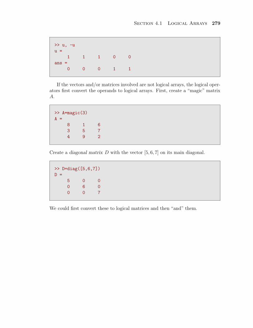
>> u, ~uu =
1 1 1 0 0ans =
0 0 0 1 1
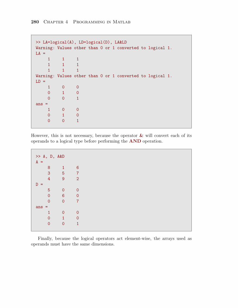
If the vectors and/or matrices involved are not logical arrays, the logical oper-ators first convert the operands to logical arrays. First, create a “magic” matrixA.
>> A=magic(3)A =
8 1 63 5 74 9 2
Create a diagonal matrix D with the vector [5, 6, 7] on its main diagonal.
>> D=diag([5,6,7])D =
5 0 00 6 00 0 7
We could first convert these to logical matrices and then “and” them.
280 Chapter 4 Programming in Matlab
>> LA=logical(A), LD=logical(D), LA&LDWarning: Values other than 0 or 1 converted to logical 1.LA =
1 1 11 1 11 1 1
Warning: Values other than 0 or 1 converted to logical 1.LD =
1 0 00 1 00 0 1
ans =1 0 00 1 00 0 1
However, this is not necessary, because the operator & will convert each of itsoperands to a logical type before performing the AND operation.
>> A, D, A&DA =
8 1 63 5 74 9 2
D =5 0 00 6 00 0 7
ans =1 0 00 1 00 0 1
Finally, because the logical operators act element-wise, the arrays used asoperands must have the same dimensions.
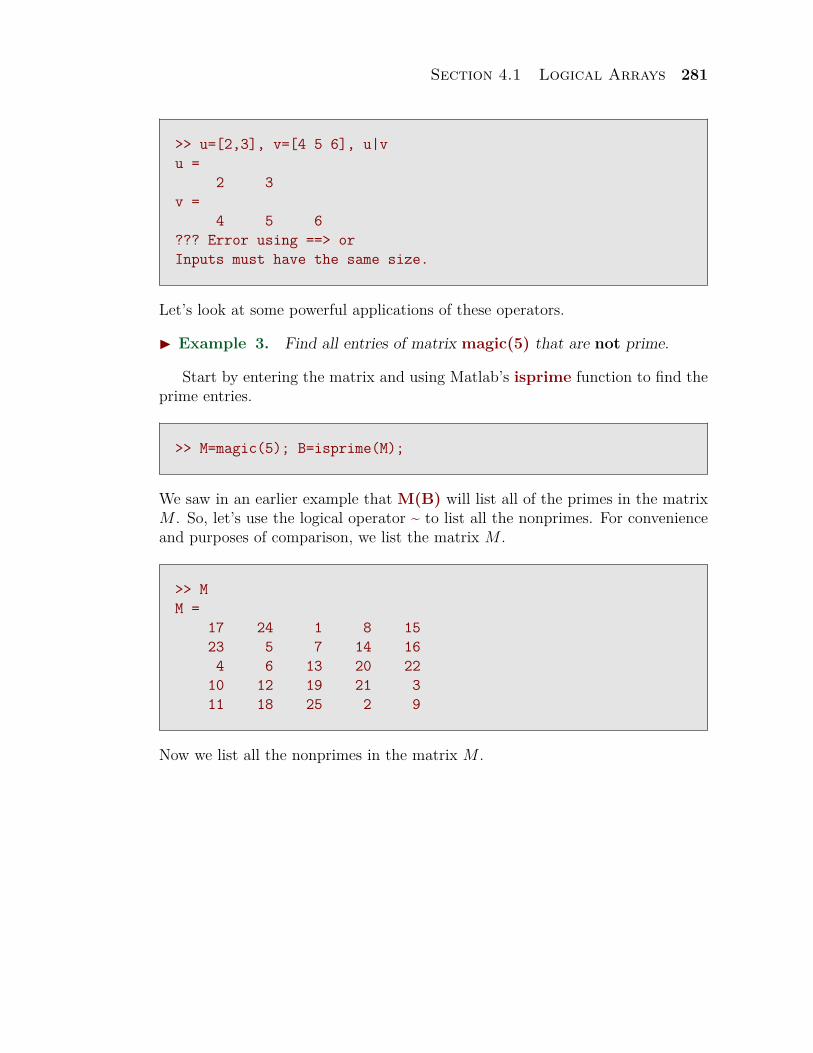
Section 4.1 Logical Arrays 281
>> u=[2,3], v=[4 5 6], u|vu =
2 3v =
4 5 6??? Error using ==> orInputs must have the same size.
Let’s look at some powerful applications of these operators.
I Example 3. Find all entries of matrix magic(5) that are not prime.
Start by entering the matrix and using Matlab’s isprime function to find theprime entries.
>> M=magic(5); B=isprime(M);
We saw in an earlier example that M(B) will list all of the primes in the matrixM . So, let’s use the logical operator ~ to list all the nonprimes. For convenienceand purposes of comparison, we list the matrix M .
>> MM =
17 24 1 8 1523 5 7 14 164 6 13 20 22
10 12 19 21 311 18 25 2 9
Now we list all the nonprimes in the matrix M .
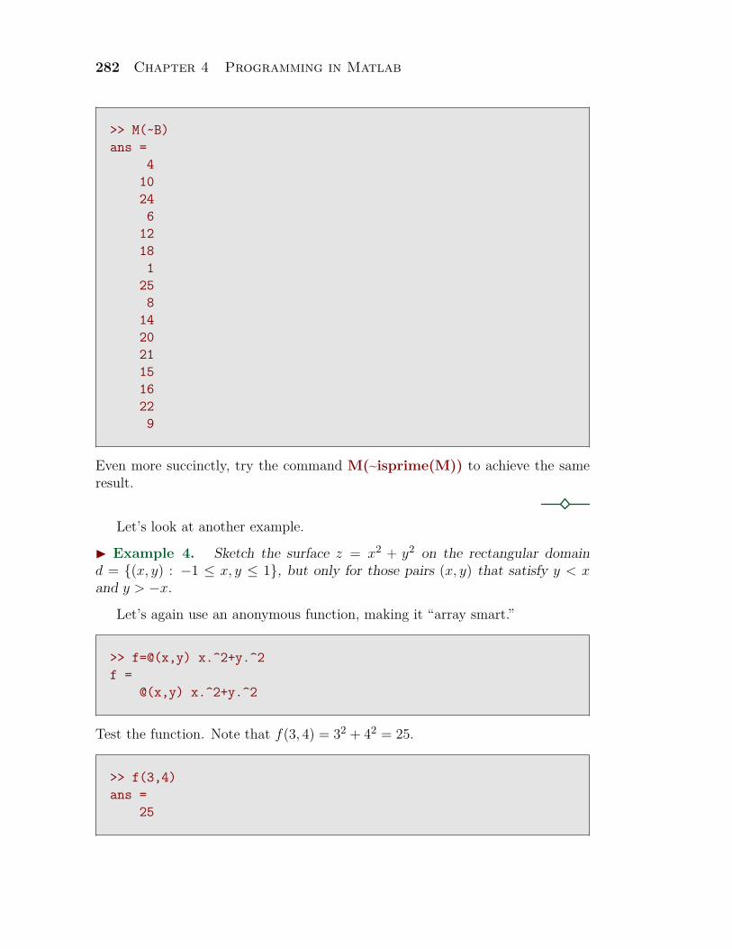
282 Chapter 4 Programming in Matlab
>> M(~B)ans =
410246
12181
258
1420211516229
Even more succinctly, try the command M(~isprime(M)) to achieve the sameresult.
Let’s look at another example.
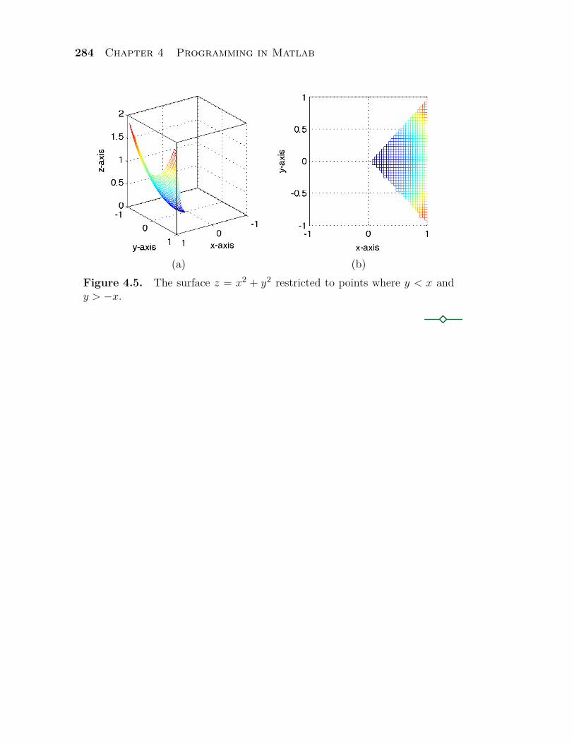
I Example 4. Sketch the surface z = x2 + y2 on the rectangular domaind = {(x, y) : −1 ≤ x, y ≤ 1}, but only for those pairs (x, y) that satisfy y < xand y > −x.
Let’s again use an anonymous function, making it “array smart.”
>> f=@(x,y) x.^2+y.^2f =
@(x,y) x.^2+y.^2
Test the function. Note that f(3, 4) = 32 + 42 = 25.
>> f(3,4)ans =
25
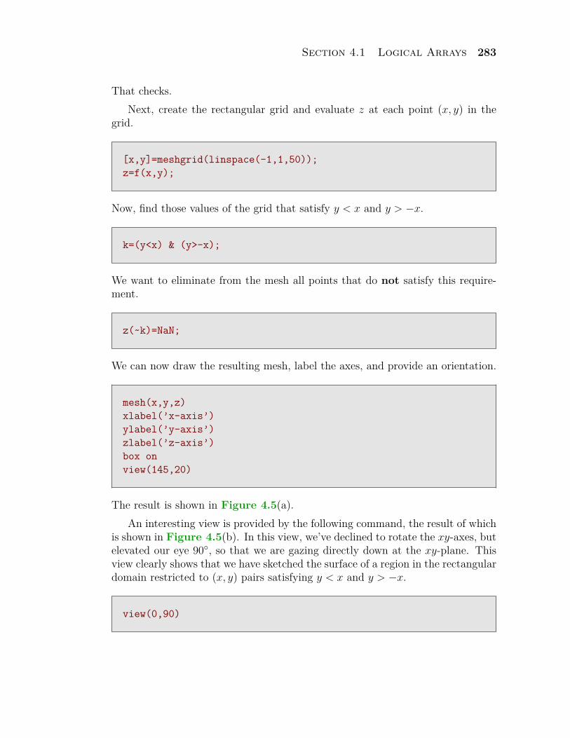
Section 4.1 Logical Arrays 283
That checks.Next, create the rectangular grid and evaluate z at each point (x, y) in the
grid.
[x,y]=meshgrid(linspace(-1,1,50));z=f(x,y);
Now, find those values of the grid that satisfy y < x and y > −x.
k=(y<x) & (y>-x);
We want to eliminate from the mesh all points that do not satisfy this require-ment.
z(~k)=NaN;
We can now draw the resulting mesh, label the axes, and provide an orientation.
mesh(x,y,z)xlabel(’x-axis’)ylabel(’y-axis’)zlabel(’z-axis’)box onview(145,20)
The result is shown in Figure 4.5(a).An interesting view is provided by the following command, the result of which
is shown in Figure 4.5(b). In this view, we’ve declined to rotate the xy-axes, butelevated our eye 90◦, so that we are gazing directly down at the xy-plane. Thisview clearly shows that we have sketched the surface of a region in the rectangulardomain restricted to (x, y) pairs satisfying y < x and y > −x.
view(0,90)
284 Chapter 4 Programming in Matlab
(a) (b)Figure 4.5. The surface z = x2 + y2 restricted to points where y < x andy > −x.
Section 4.1 Logical Arrays 285
4.1 Exercises
In Exercises 1-6, first enter the fol-lowing vectors.
>> v=[1,3,5,7], w=[5,2,5,4]v =
1 3 5 7w =
5 2 5 4
In each exercise, first predict the out-put of the given command, then val-idate your response with the appro-priate Matlab command. Note: Theidea here is not to simply enter thecommand. Rather, spend some timethinking, then predict the output be-fore you enter the command to verifyyour conclusion.
1. v>w
2. v>=w
3. v<=w
4. v<w
5. v==w
6. v~=w
Store the following “magic” matrix inthe variable A.
Copyrighted material. See: http://msenux.redwoods.edu/IntAlgText/3
>> A=magic(5)A =
17 24 1 8 1523 5 7 14 164 6 13 20 22
10 12 19 21 311 18 25 2 9
In Exercises 7-12, first predict theoutput of the given command, thenvalidate your response with the appro-priate Matlab command. Note: Theidea here is not to simply enter thecommand. Rather, spend some timethinking, then predict the output be-fore you enter the command to verifyyour conclusion.
7.
>> A>14
8.
>> A<=12
9.
>> (A>3) & (A<=20)
10.
286 Chapter 4 Programming in Matlab
>> (A<5) | (A>=21)
11.
>> ~(A<=6)
12.
>> (A>6) & ~(A>8)
13. Set P=pascal(5). Write a Mat-lab command that will list all entriesof matrix P that are less than 20 butnot equal to 1.
14. Set P=pascal(5). Write a Mat-lab command that will list all entriesof matrix P that are not equal to 1.
15. Set P=pascal(5). Write a Mat-lab command that will list all entriesof matrix P that are less than or equalto 4 or greater than 20.
16. Set P=pascal(5). Write a Mat-lab command that will list all entriesof matrix P that are greater than 3but not greater than 35.
When a and b are positive integers,the Matlab command mod(a,b) re-turns the remainder when a is dividedby b. Use this command to producethe requested entries of the given ma-trix in Exercises 17-20.
17. Set A=magic(4). Write a Mat-
lab command that will return all en-tries of matrix A that are divisible by2. Hint: An integer k is divisible by2 if the remainder is zero when k isdivided by 2.
18. Set A=magic(4). Write a Mat-lab command that will return all en-tries of matrix A that are odd inte-gers. Hint: A integer k is odd if itsremainder is 1 when k is divided by 2.
19. Set A=magic(4). Write a Mat-lab command that will return all en-tries of matrix A that are divisible by3.
20. Set A=magic(4). Write a Mat-lab command that will return all en-tries of matrix A that are divisible by5.
21. Execute the following commandto list the primes less than or equal to100.
>> primes(100)
Secondly, create a vector u hold-ing the integers from 1 to 100, inclu-sive. Use Matlab’s isprime commandand logical indexing to pick out andlist all the primes in vector u. Com-pare the results.
22. Create a vector u holding theintegers from 100 to 1000, inclusive.Use Matlab’s isprime command andlogical indexing to pick out all the primesin vector u. Use Matlab’s max com-mand on the result to find the largest
Section 4.1 Logical Arrays 287
prime between 100 and 1000.
In Exercises 23-26, perform each ofthe following tasks for the given func-tion.
i. Write an “array smart” anonymousfunction f for the given function.Test your anonymous function be-fore proceeding.
ii. Set x=linspace(-10,10,200) andevaluate the function with y=f(x).
iii. Use the plot(x,y) command to plotthe function.
iv. Use axis([-10,10,-10,10]) to setthe window boundaries.
v. Use logical indexing to set all ofthe complex entries in the vectory to NaN. Open a second figurewindow with the command figure.Replot the result and reset the win-dow boundaries as above, if neces-sary. Add axis labels and a titleand turn the grid on.
23. f(x) = 2 +√
x + 5
24. f(x) = 3−√
x− 3
25. f(x) =√
9− x2
26. f(x) =√
x2 − 25
In Exercises 27-30, use “advancedplanning” to plot the given functionon a subset of the domain [−10, 10]to avoid complex entries when eval-uating the given function. In eachcase, set the window boundaries withthe command axis([-10,10,-10,10]),turn on the grid, and add axes labelsand a title.
27. The function in Exercise 23.
28. The function in Exercise 24.
29. The function in Exercise 25.
30. The function in Exercise 26.
In Exercises 31-34, perform each ofthe following tasks for the given func-tion.
i. Write an “array smart” anonymousfunction f for the given function.Test your anonymous function be-fore proceeding.
ii. Set:
x=linspace(-3,3,40);y=x;[x,y]=meshgrid(x,y);
Evaluate the function with z=f(x,y).iii. Use mesh(x,y,z) to plot the sur-
face defined by the function.iv. Use logical indexing to set all of
the complex entries in the vectorz to NaN. Open a second figurewindow with the command figure.Replot the surface. Add axis la-bels and a title.
31. f(x, y) =√
1 + x
32. f(x, y) =√
1− y
33. f(x, y) =√
9− x2 − y2
34. f(x, y) =√
x2 + y2 − 1
In Exercises 35-40, perform each ofthe following tasks for the given func-
288 Chapter 4 Programming in Matlab
tion.
i. Write an “array smart” anonymousfunction f for the given function.Test your anonymous function be-fore proceeding.
ii. Set:
x=linspace(-3,3,40);y=x;[x,y]=meshgrid(x,y);
Evaluate the function with z=f(x,y).iii. Use logical indexing to replace all
entries in z with NaN that do notsatisfy the given constraint.
iv. Use mesh(x,y,z) to plot the sur-face defined by the function andconstraint. Add axis labels and atitle.
v. Open a second figure window withthe command figure. Replot thesurface and orient the view withview(0,90). Add axis labels anda title. Does the pictured regionsatisfy the given constraint?
35. f(x, y) = 12− x− y where
x > −1.
36. f(x, y) = 10− 2x + y where
y ≤ 3.
37. f(x, y) = 14 + x− 2y where
x + y < 0.
38. f(x, y) = 14 + x− 2y where
x− y ≥ 0.
39. f(x, y) = 11− 2x + 2y where
x + y < 0 and x ≥ −2.
40. f(x, y) = 10 + 2x− 3y where
x− 2y ≤ 0 or y ≤ 0.
Section 4.1 Logical Arrays 289
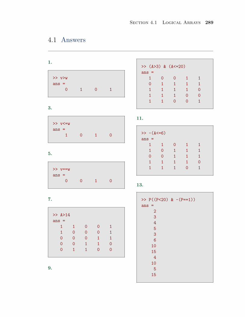
4.1 Answers
1.
>> v>wans =
0 1 0 1
3.
>> v<=wans =
1 0 1 0
5.
>> v==wans =
0 0 1 0
7.
>> A>14ans =
1 1 0 0 11 0 0 0 10 0 0 1 10 0 1 1 00 1 1 0 0
9.
>> (A>3) & (A<=20)ans =
1 0 0 1 10 1 1 1 11 1 1 1 01 1 1 0 01 1 0 0 1
11.
>> ~(A<=6)ans =
1 1 0 1 11 0 1 1 10 0 1 1 11 1 1 1 01 1 1 0 1
13.
>> P((P<20) & ~(P==1))ans =
234536
10154
105
15
290 Chapter 4 Programming in Matlab
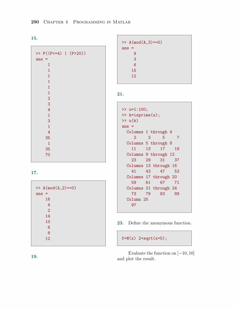
15.
>> P((P<=4) | (P>20))ans =
1111112341314
351
3570
17.
>> A(mod(A,2)==0)ans =
1642
141068
12
19.
>> A(mod(A,3)==0)ans =
936
1512
21.
>> u=1:100;>> k=isprime(u);>> u(k)ans =
Columns 1 through 42 3 5 7
Columns 5 through 811 13 17 19
Columns 9 through 1223 29 31 37
Columns 13 through 1641 43 47 53
Columns 17 through 2059 61 67 71
Columns 21 through 2473 79 83 89
Column 2597
23. Define the anonymous function.
f=@(x) 2+sqrt(x+5);
Evaluate the function on [−10, 10]and plot the result.
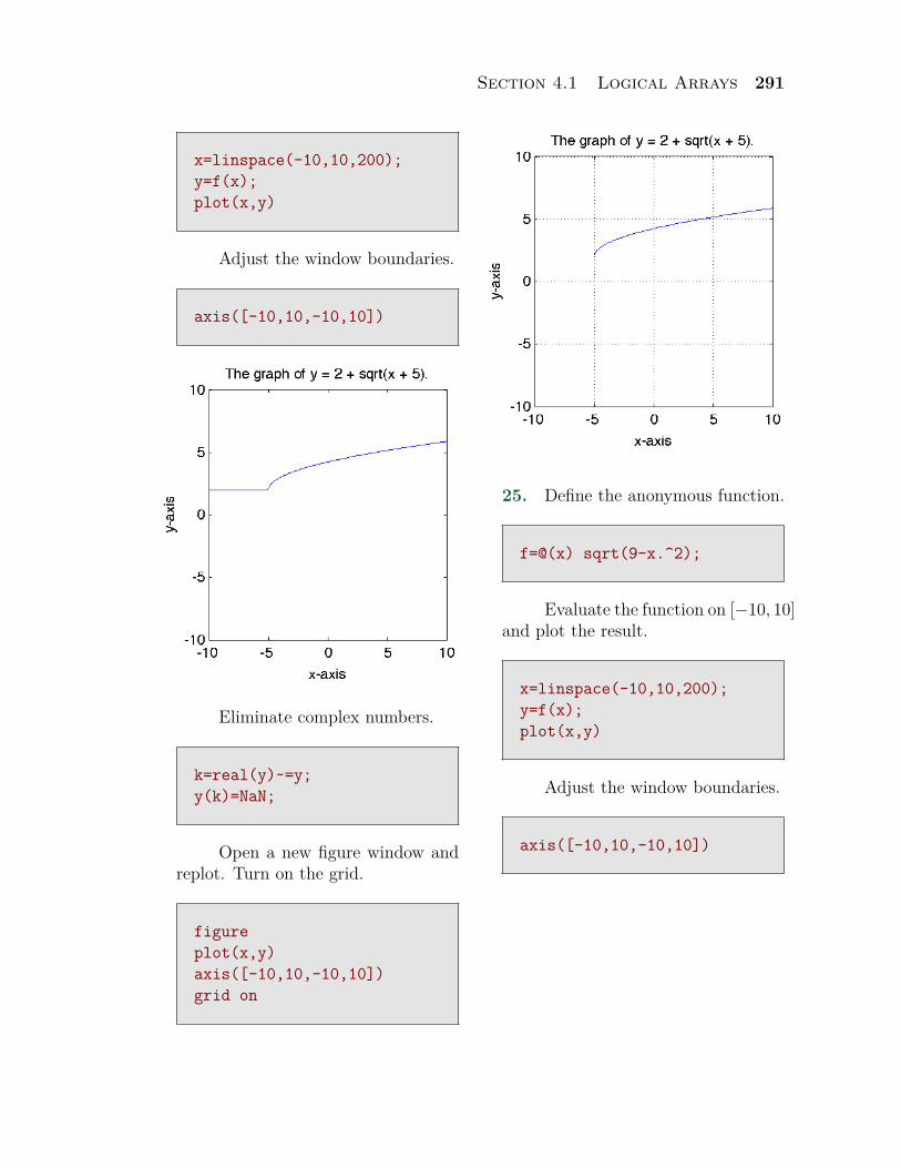
Section 4.1 Logical Arrays 291
x=linspace(-10,10,200);y=f(x);plot(x,y)
Adjust the window boundaries.
axis([-10,10,-10,10])
Eliminate complex numbers.
k=real(y)~=y;y(k)=NaN;
Open a new figure window andreplot. Turn on the grid.
figureplot(x,y)axis([-10,10,-10,10])grid on
25. Define the anonymous function.
f=@(x) sqrt(9-x.^2);
Evaluate the function on [−10, 10]and plot the result.
x=linspace(-10,10,200);y=f(x);plot(x,y)
Adjust the window boundaries.
axis([-10,10,-10,10])
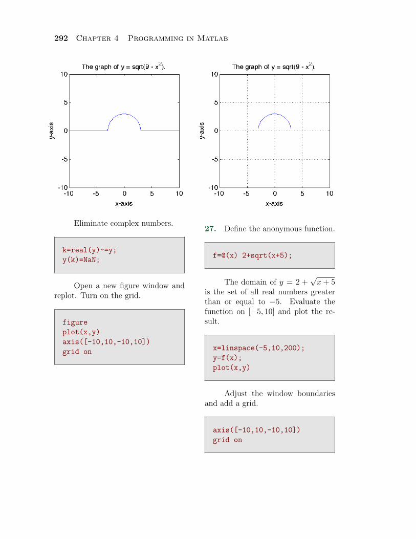
292 Chapter 4 Programming in Matlab
Eliminate complex numbers.
k=real(y)~=y;y(k)=NaN;
Open a new figure window andreplot. Turn on the grid.
figureplot(x,y)axis([-10,10,-10,10])grid on
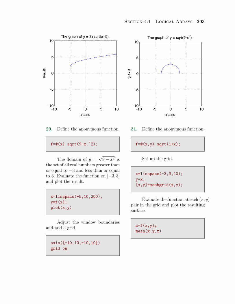
27. Define the anonymous function.
f=@(x) 2+sqrt(x+5);
The domain of y = 2 +√
x + 5is the set of all real numbers greaterthan or equal to −5. Evaluate thefunction on [−5, 10] and plot the re-sult.
x=linspace(-5,10,200);y=f(x);plot(x,y)
Adjust the window boundariesand add a grid.
axis([-10,10,-10,10])grid on
Section 4.1 Logical Arrays 293
29. Define the anonymous function.
f=@(x) sqrt(9-x.^2);
The domain of y =√
9− x2 isthe set of all real numbers greater thanor equal to −3 and less than or equalto 3. Evaluate the function on [−3, 3]and plot the result.
x=linspace(-5,10,200);y=f(x);plot(x,y)
Adjust the window boundariesand add a grid.
axis([-10,10,-10,10])grid on
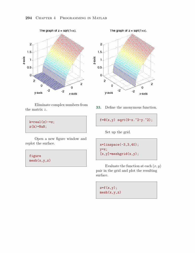
31. Define the anonymous function.
f=@(x,y) sqrt(1+x);
Set up the grid.
x=linspace(-3,3,40);y=x;[x,y]=meshgrid(x,y);
Evaluate the function at each (x, y)pair in the grid and plot the resultingsurface.
z=f(x,y);mesh(x,y,z)
294 Chapter 4 Programming in Matlab
Eliminate complex numbers fromthe matrix z.
k=real(z)~=z;z(k)=NaN;
Open a new figure window andreplot the surface.
figuremesh(x,y,z)
33. Define the anonymous function.
f=@(x,y) sqrt(9-x.^2-y.^2);
Set up the grid.
x=linspace(-3,3,40);y=x;[x,y]=meshgrid(x,y);
Evaluate the function at each (x, y)pair in the grid and plot the resultingsurface.
z=f(x,y);mesh(x,y,z)

Section 4.1 Logical Arrays 295
Eliminate complex numbers fromthe matrix z.
k=real(z)~=z;z(k)=NaN;
Open a new figure window andreplot the surface.
figuremesh(x,y,z)
35. Define the anonymous function.
f=@(x,y) 12-x-y;
Set up the grid.
x=linspace(-3,3,40);y=x;[x,y]=meshgrid(x,y);
Evaluate the function at each (x, y)pair in the grid.
z=f(x,y);
Determine where x > −1 andset all entries in z equal to NaN wherethis contraint is not satisfied.
k=x>-1;z(~k)=NaN;
296 Chapter 4 Programming in Matlab
Draw the surface, adjust the ori-entation, and turn the box on for depth.
mesh(x,y,z)view(130,30)box on
Open a new figure window, re-plot, and adjust the view so that theeye stares down the z-axis directly atthe xy-plane.
figuremesh(x,y,z)view(0,90)
37. Define the anonymous function.
f=@(x,y) 14+x-2*y;
Set up the grid.
x=linspace(-3,3,40);y=x;[x,y]=meshgrid(x,y);
Evaluate the function at each (x, y)pair in the grid.
z=f(x,y);
Determine where x > −1 andset all entries in z equal to NaN wherethis contraint is not satisfied.
k=x+y<0;z(~k)=NaN;
Section 4.1 Logical Arrays 297
Draw the surface, adjust the ori-entation, and turn the box on for depth.
mesh(x,y,z)view(130,30)box on
Open a new figure window, re-plot, and adjust the view so that theeye stares down the z-axis directly atthe xy-plane.
figuremesh(x,y,z)view(0,90)
39. Define the anonymous function.
f=@(x,y) 11-2*x+2*y;
Set up the grid.
x=linspace(-3,3,40);y=x;[x,y]=meshgrid(x,y);
Evaluate the function at each (x, y)pair in the grid.
z=f(x,y);
Determine where x > −1 andset all entries in z equal to NaN wherethis contraint is not satisfied.
z=f(x,y);k=(x+y<0) & (x>=-2);z(~k)=NaN;
298 Chapter 4 Programming in Matlab
Draw the surface, adjust the ori-entation, and turn the box on for depth.
mesh(x,y,z)view(130,30)box on
Open a new figure window, re-plot, and adjust the view so that theeye stares down the z-axis directly atthe xy-plane.
figuremesh(x,y,z)view(0,90)
Section 4.2 Control Structures in Matlab 299
4.2 Control Structures in MatlabIn this section we will discuss the control structures offered by the Matlab
programming language that allow us to add more levels of complexity to thesimple programs we have written thus far. Without further ado and fanfare, let’sbegin.
IfIf evaluates a logical expression and executes a block of statements based onwhether the logical expressions evaluates to true (logical 1) or false (logical 0).The basic structure is as follows.
if logical_expressionstatements
end
If the logical_expression evaluates as true (logical 1), then the block of state-ments that follow if logical_expression are executed, otherwise the statementsare skipped and program control is transferred to the first statement that followsend. Let’s look at an example of this control structure’s use.
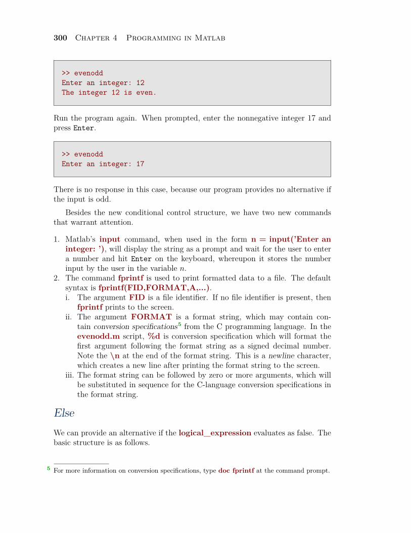
Matlab’s rem(a,b) returns the remainder when a is divided by b. Thus, if a isan even integer, then rem(a,2) will equal zero. What follows is a short programto test if an integer is even. Open the Matlab editor, enter the following script,then save the file as evenodd.m.
n = input(’Enter an integer: ’);if (rem(n,2)==0)
fprintf(’The integer %d is even.\n’, n)end
Return to the command window and run the script by entering evenodd atthe Matlab prompt. Matlab responds by asking you to enter an integer. As aresponse, enter the integer 12 and press Enter.
Copyrighted material. See: http://msenux.redwoods.edu/Math4Textbook/4
300 Chapter 4 Programming in Matlab
>> evenoddEnter an integer: 12The integer 12 is even.
Run the program again. When prompted, enter the nonnegative integer 17 andpress Enter.
>> evenoddEnter an integer: 17
There is no response in this case, because our program provides no alternative ifthe input is odd.
Besides the new conditional control structure, we have two new commandsthat warrant attention.
1. Matlab’s input command, when used in the form n = input(’Enter aninteger: ’), will display the string as a prompt and wait for the user to entera number and hit Enter on the keyboard, whereupon it stores the numberinput by the user in the variable n.
2. The command fprintf is used to print formatted data to a file. The defaultsyntax is fprintf(FID,FORMAT,A,...).i. The argument FID is a file identifier. If no file identifier is present, then
fprintf prints to the screen.ii. The argument FORMAT is a format string, which may contain con-
tain conversion specifications5 from the C programming language. In theevenodd.m script, %d is conversion specification which will format thefirst argument following the format string as a signed decimal number.Note the \n at the end of the format string. This is a newline character,which creates a new line after printing the format string to the screen.
iii. The format string can be followed by zero or more arguments, which willbe substituted in sequence for the C-language conversion specifications inthe format string.
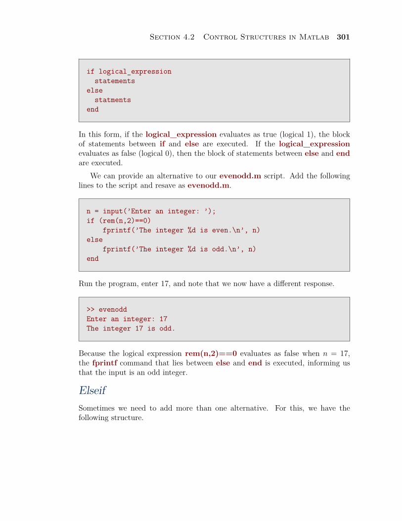
ElseWe can provide an alternative if the logical_expression evaluates as false. Thebasic structure is as follows.
For more information on conversion specifications, type doc fprintf at the command prompt.5
Section 4.2 Control Structures in Matlab 301
if logical_expressionstatements
elsestatments
end
In this form, if the logical_expression evaluates as true (logical 1), the blockof statements between if and else are executed. If the logical_expressionevaluates as false (logical 0), then the block of statements between else and endare executed.
We can provide an alternative to our evenodd.m script. Add the followinglines to the script and resave as evenodd.m.
n = input(’Enter an integer: ’);if (rem(n,2)==0)
fprintf(’The integer %d is even.\n’, n)else
fprintf(’The integer %d is odd.\n’, n)end
Run the program, enter 17, and note that we now have a different response.
>> evenoddEnter an integer: 17The integer 17 is odd.
Because the logical expression rem(n,2)==0 evaluates as false when n = 17,the fprintf command that lies between else and end is executed, informing usthat the input is an odd integer.
ElseifSometimes we need to add more than one alternative. For this, we have thefollowing structure.
302 Chapter 4 Programming in Matlab
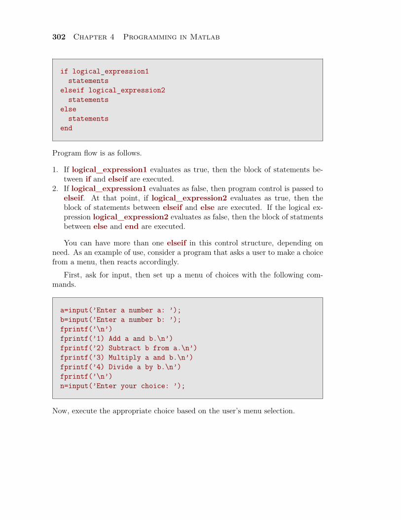
if logical_expression1statements
elseif logical_expression2statements
elsestatements
end
Program flow is as follows.
1. If logical_expression1 evaluates as true, then the block of statements be-tween if and elseif are executed.
2. If logical_expression1 evaluates as false, then program control is passed toelseif. At that point, if logical_expression2 evaluates as true, then theblock of statements between elseif and else are executed. If the logical ex-pression logical_expression2 evaluates as false, then the block of statmentsbetween else and end are executed.
You can have more than one elseif in this control structure, depending onneed. As an example of use, consider a program that asks a user to make a choicefrom a menu, then reacts accordingly.
First, ask for input, then set up a menu of choices with the following com-mands.
a=input(’Enter a number a: ’);b=input(’Enter a number b: ’);fprintf(’\n’)fprintf(’1) Add a and b.\n’)fprintf(’2) Subtract b from a.\n’)fprintf(’3) Multiply a and b.\n’)fprintf(’4) Divide a by b.\n’)fprintf(’\n’)n=input(’Enter your choice: ’);
Now, execute the appropriate choice based on the user’s menu selection.
Section 4.2 Control Structures in Matlab 303
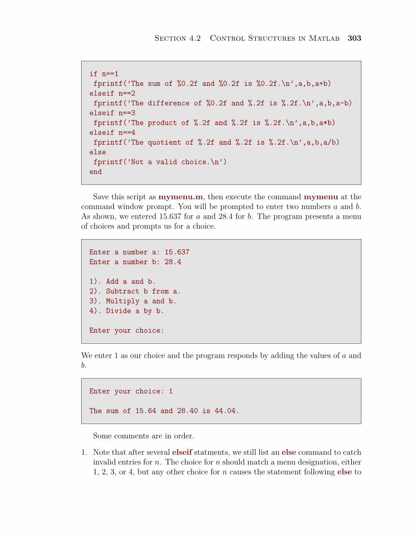
if n==1fprintf(’The sum of %0.2f and %0.2f is %0.2f.\n’,a,b,a+b)
elseif n==2fprintf(’The difference of %0.2f and %.2f is %.2f.\n’,a,b,a-b)
elseif n==3fprintf(’The product of %.2f and %.2f is %.2f.\n’,a,b,a*b)
elseif n==4fprintf(’The quotient of %.2f and %.2f is %.2f.\n’,a,b,a/b)
elsefprintf(’Not a valid choice.\n’)
end
Save this script as mymenu.m, then execute the command mymenu at thecommand window prompt. You will be prompted to enter two numbers a and b.As shown, we entered 15.637 for a and 28.4 for b. The program presents a menuof choices and prompts us for a choice.
Enter a number a: 15.637Enter a number b: 28.4
1). Add a and b.2). Subtract b from a.3). Multiply a and b.4). Divide a by b.
Enter your choice:
We enter 1 as our choice and the program responds by adding the values of a andb.
Enter your choice: 1
The sum of 15.64 and 28.40 is 44.04.
Some comments are in order.
1. Note that after several elseif statments, we still list an else command to catchinvalid entries for n. The choice for n should match a menu designation, either1, 2, 3, or 4, but any other choice for n causes the statement following else to
304 Chapter 4 Programming in Matlab
be executed. This is a good programming practice, having a sort of “otherwiseblock ’ as a catchall for unexpected responses by the user.
2. We use the conversion specification %0.2f in this example, which outputs anumber in fixed point format with two decimal places. Note that this resultsin rounding in the output of numbers with more than two decimal places.
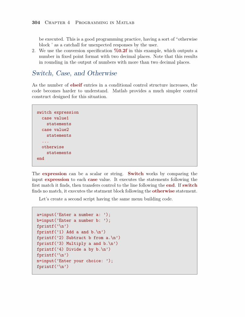
Switch, Case, and OtherwiseAs the number of elseif entries in a conditional control structure increases, thecode becomes harder to understand. Matlab provides a much simpler controlconstruct designed for this situation.
switch expressioncase value1
statementscase value2
statements...otherwise
statementsend
The expression can be a scalar or string. Switch works by comparing theinput expression to each case value. It executes the statements following thefirst match it finds, then transfers control to the line following the end. If switchfinds no match, it executes the statment block following the otherwise statement.
Let’s create a second script having the same menu building code.
a=input(’Enter a number a: ’);b=input(’Enter a number b: ’);fprintf(’\n’)fprintf(’1) Add a and b.\n’)fprintf(’2) Subtract b from a.\n’)fprintf(’3) Multiply a and b.\n’)fprintf(’4) Divide a by b.\n’)fprintf(’\n’)n=input(’Enter your choice: ’);fprintf(’\n’)
Section 4.2 Control Structures in Matlab 305
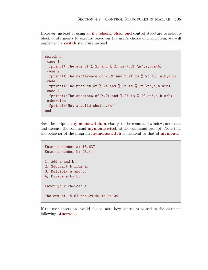
However, instead of using an if ...elseif...else...end control structure to select ablock of statments to execute based on the user’s choice of menu item, we willimplement a switch structure instead.
switch ncase 1fprintf(’The sum of %.2f and %.2f is %.2f.\n’,a,b,a+b)
case 2fprintf(’The difference of %.2f and %.2f is %.2f.\n’,a,b,a-b)
case 3fprintf(’The product of %.2f and %.2f is %.2f.\n’,a,b,a*b)
case 4fprintf(’The quotient of %.2f and %.2f is %.2f.\n’,a,b,a/b)
otherwisefprintf(’Not a valid choice.\n’)
end
Save the script as mymenuswitch.m, change to the command window, and enterand execute the command mymenuswitch at the command prompt. Note thatthe behavior of the program mymenuswitch is identical to that of mymenu.
Enter a number a: 15.637Enter a number b: 28.4
1) Add a and b.2) Subtract b from a.3) Multiply a and b.4) Divide a by b.
Enter your choice: 1
The sum of 15.64 and 28.40 is 44.04.
If the user enters an invalid choice, note how control is passed to the statmentfollowing otherwise.
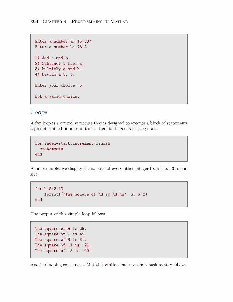
306 Chapter 4 Programming in Matlab
Enter a number a: 15.637Enter a number b: 28.4
1) Add a and b.2) Subtract b from a.3) Multiply a and b.4) Divide a by b.
Enter your choice: 5
Not a valid choice.
LoopsA for loop is a control structure that is designed to execute a block of statementsa predetermined number of times. Here is its general use syntax.
for index=start:increment:finishstatements
end
As an example, we display the squares of every other integer from 5 to 13, inclu-sive.
for k=5:2:13fprintf(’The square of %d is %d.\n’, k, k^2)
end
The output of this simple loop follows.
The square of 5 is 25.The square of 7 is 49.The square of 9 is 81.The square of 11 is 121.The square of 13 is 169.
Another looping construct is Matlab’s while structure who’s basic syntax follows.
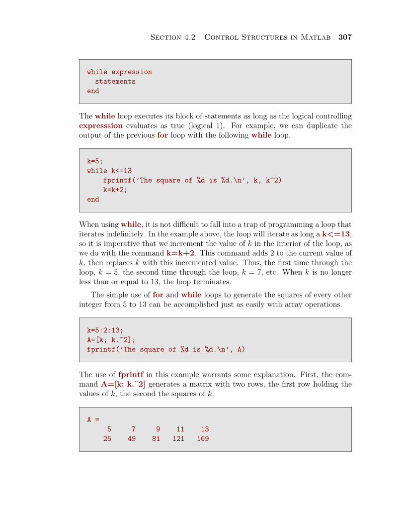
Section 4.2 Control Structures in Matlab 307
while expressionstatements
end
The while loop executes its block of statements as long as the logical controllingexpresssion evaluates as true (logical 1). For example, we can duplicate theoutput of the previous for loop with the following while loop.
k=5;while k<=13
fprintf(’The square of %d is %d.\n’, k, k^2)k=k+2;
end
When using while, it is not difficult to fall into a trap of programming a loop thatiterates indefinitely. In the example above, the loop will iterate as long a k<=13,so it is imperative that we increment the value of k in the interior of the loop, aswe do with the command k=k+2. This command adds 2 to the current value ofk, then replaces k with this incremented value. Thus, the first time through theloop, k = 5, the second time through the loop, k = 7, etc. When k is no longerless than or equal to 13, the loop terminates.
The simple use of for and while loops to generate the squares of every otherinteger from 5 to 13 can be accomplished just as easily with array operations.
k=5:2:13;A=[k; k.^2];fprintf(’The square of %d is %d.\n’, A)
The use of fprintf in this example warrants some explanation. First, the com-mand A=[k; k.^2] generates a matrix with two rows, the first row holding thevalues of k, the second the squares of k.
A =5 7 9 11 13
25 49 81 121 169
308 Chapter 4 Programming in Matlab
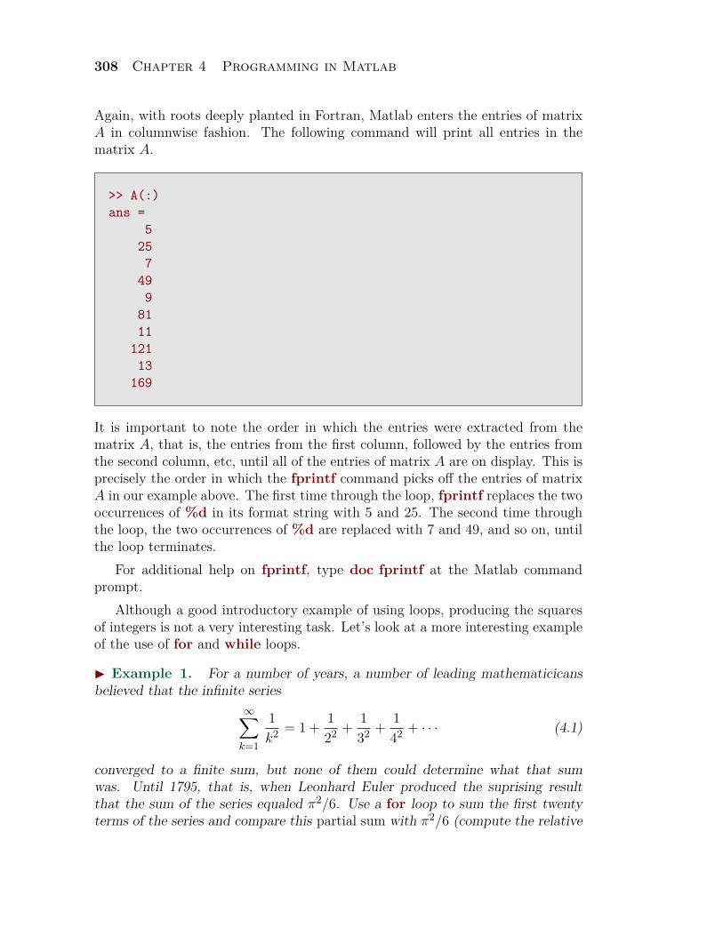
Again, with roots deeply planted in Fortran, Matlab enters the entries of matrixA in columnwise fashion. The following command will print all entries in thematrix A.
>> A(:)ans =
5257
499
8111
12113
169
It is important to note the order in which the entries were extracted from thematrix A, that is, the entries from the first column, followed by the entries fromthe second column, etc, until all of the entries of matrix A are on display. This isprecisely the order in which the fprintf command picks off the entries of matrixA in our example above. The first time through the loop, fprintf replaces the twooccurrences of %d in its format string with 5 and 25. The second time throughthe loop, the two occurrences of %d are replaced with 7 and 49, and so on, untilthe loop terminates.
For additional help on fprintf, type doc fprintf at the Matlab commandprompt.
Although a good introductory example of using loops, producing the squaresof integers is not a very interesting task. Let’s look at a more interesting exampleof the use of for and while loops.
I Example 1. For a number of years, a number of leading mathematicicansbelieved that the infinite series
∞∑k=1
1k2 = 1 + 1
22 + 132 + 1
42 + · · · (4.1)
converged to a finite sum, but none of them could determine what that sumwas. Until 1795, that is, when Leonhard Euler produced the suprising resultthat the sum of the series equaled π2/6. Use a for loop to sum the first twentyterms of the series and compare this partial sum with π2/6 (compute the relative
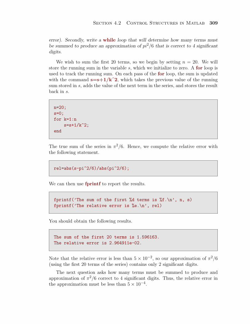
Section 4.2 Control Structures in Matlab 309
error). Secondly, write a while loop that will determine how many terms mustbe summed to produce an approximation of pi2/6 that is correct to 4 significantdigits.
We wish to sum the first 20 terms, so we begin by setting n = 20. We willstore the running sum in the variable s, which we initialize to zero. A for loop isused to track the running sum. On each pass of the for loop, the sum is updatedwith the command s=s+1/k^2, which takes the previous value of the runningsum stored in s, adds the value of the next term in the series, and stores the resultback in s.
n=20;s=0;for k=1:n
s=s+1/k^2;end
The true sum of the series in π2/6. Hence, we compute the relative error withthe following statement.
rel=abs(s-pi^2/6)/abs(pi^2/6);
We can then use fprintf to report the results.
fprintf(’The sum of the first %d terms is %f.\n’, n, s)fprintf(’The relative error is %e.\n’, rel)
You should obtain the following results.
The sum of the first 20 terms is 1.596163.The relative error is 2.964911e-02.
Note that the relative error is less than 5 × 10⁻², so our approximation of π2/6(using the first 20 terms of the series) contains only 2 significant digits.
The next question asks how many terms must be summed to produce andapproximation of π2/6 correct to 4 significant digits. Thus, the relative error inthe approximation must be less than 5× 10⁻⁴.
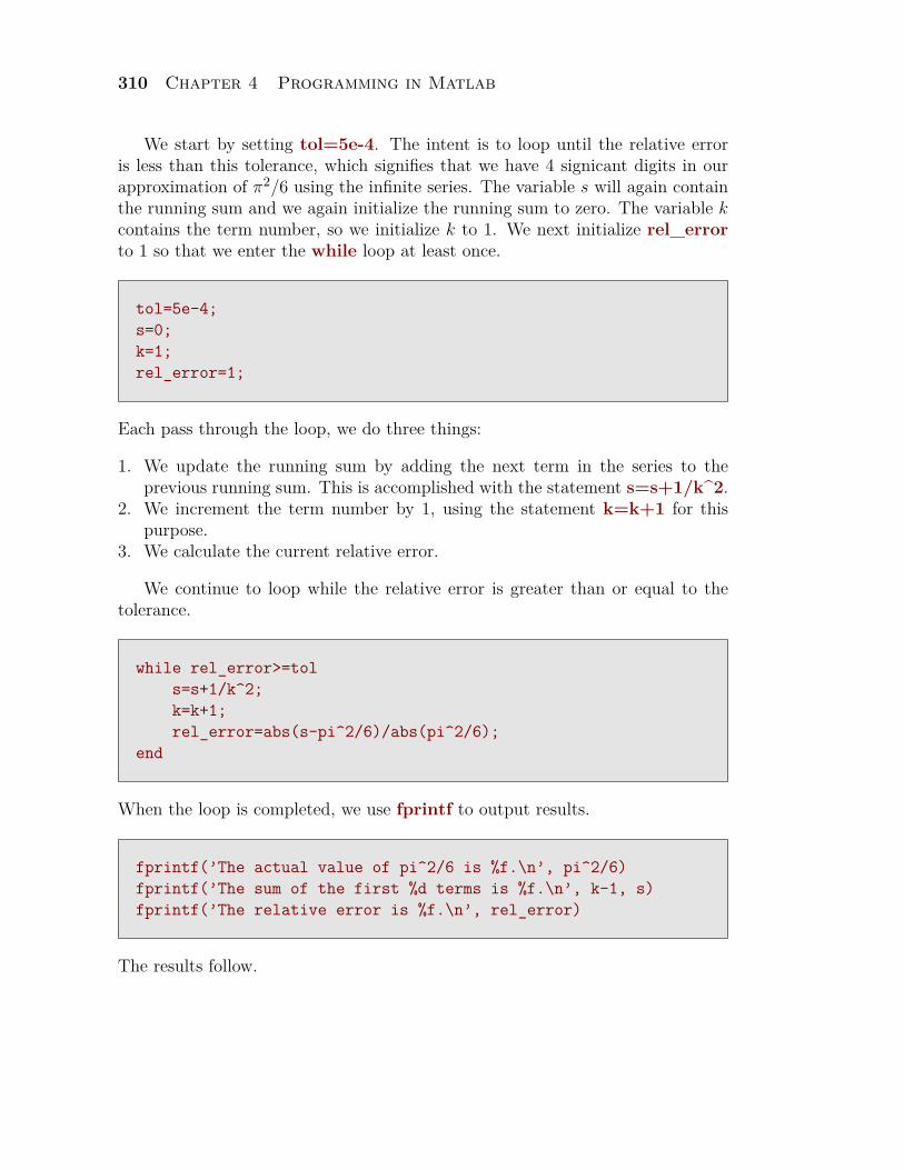
310 Chapter 4 Programming in Matlab
We start by setting tol=5e-4. The intent is to loop until the relative erroris less than this tolerance, which signifies that we have 4 signicant digits in ourapproximation of π2/6 using the infinite series. The variable s will again containthe running sum and we again initialize the running sum to zero. The variable kcontains the term number, so we initialize k to 1. We next initialize rel_errorto 1 so that we enter the while loop at least once.
tol=5e-4;s=0;k=1;rel_error=1;
Each pass through the loop, we do three things:
1. We update the running sum by adding the next term in the series to theprevious running sum. This is accomplished with the statement s=s+1/k^2.
2. We increment the term number by 1, using the statement k=k+1 for thispurpose.
3. We calculate the current relative error.
We continue to loop while the relative error is greater than or equal to thetolerance.
while rel_error>=tols=s+1/k^2;k=k+1;rel_error=abs(s-pi^2/6)/abs(pi^2/6);
end
When the loop is completed, we use fprintf to output results.
fprintf(’The actual value of pi^2/6 is %f.\n’, pi^2/6)fprintf(’The sum of the first %d terms is %f.\n’, k-1, s)fprintf(’The relative error is %f.\n’, rel_error)
The results follow.
Section 4.2 Control Structures in Matlab 311
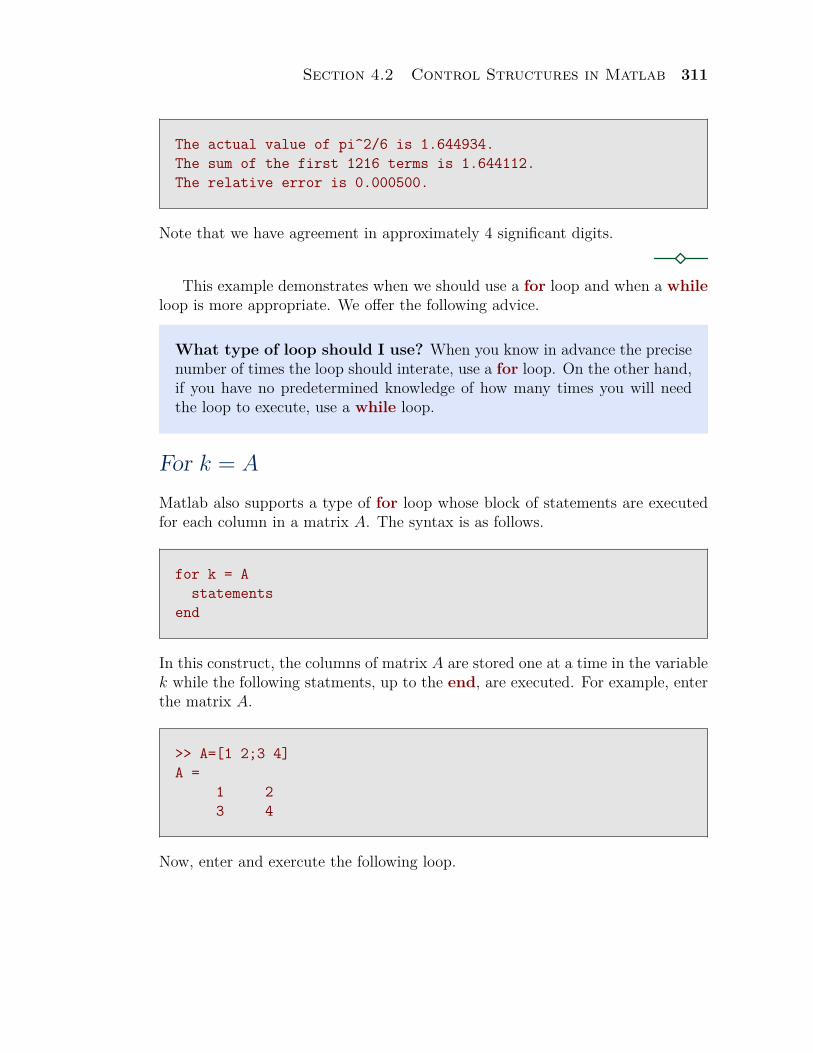
The actual value of pi^2/6 is 1.644934.The sum of the first 1216 terms is 1.644112.The relative error is 0.000500.
Note that we have agreement in approximately 4 significant digits.
This example demonstrates when we should use a for loop and when a whileloop is more appropriate. We offer the following advice.
What type of loop should I use? When you know in advance the precisenumber of times the loop should interate, use a for loop. On the other hand,if you have no predetermined knowledge of how many times you will needthe loop to execute, use a while loop.
For k = A
Matlab also supports a type of for loop whose block of statements are executedfor each column in a matrix A. The syntax is as follows.
for k = Astatements
end
In this construct, the columns of matrix A are stored one at a time in the variablek while the following statments, up to the end, are executed. For example, enterthe matrix A.
>> A=[1 2;3 4]A =
1 23 4
Now, enter and exercute the following loop.
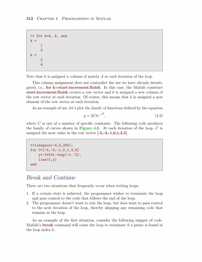
312 Chapter 4 Programming in Matlab
>> for k=A, k, endk =
13
k =24
Note that k is assigned a column of matrix A at each iteration of the loop.This column assignment does not contradict the use we have already investi-
gated, i.e., for k=start:increment:finish. In this case, the Matlab constructstart:increment:finish creates a row vector and k is assigned a new column ofthe row vector at each iteration. Of course, this means that k is assigned a newelement of the row vector at each iteration.
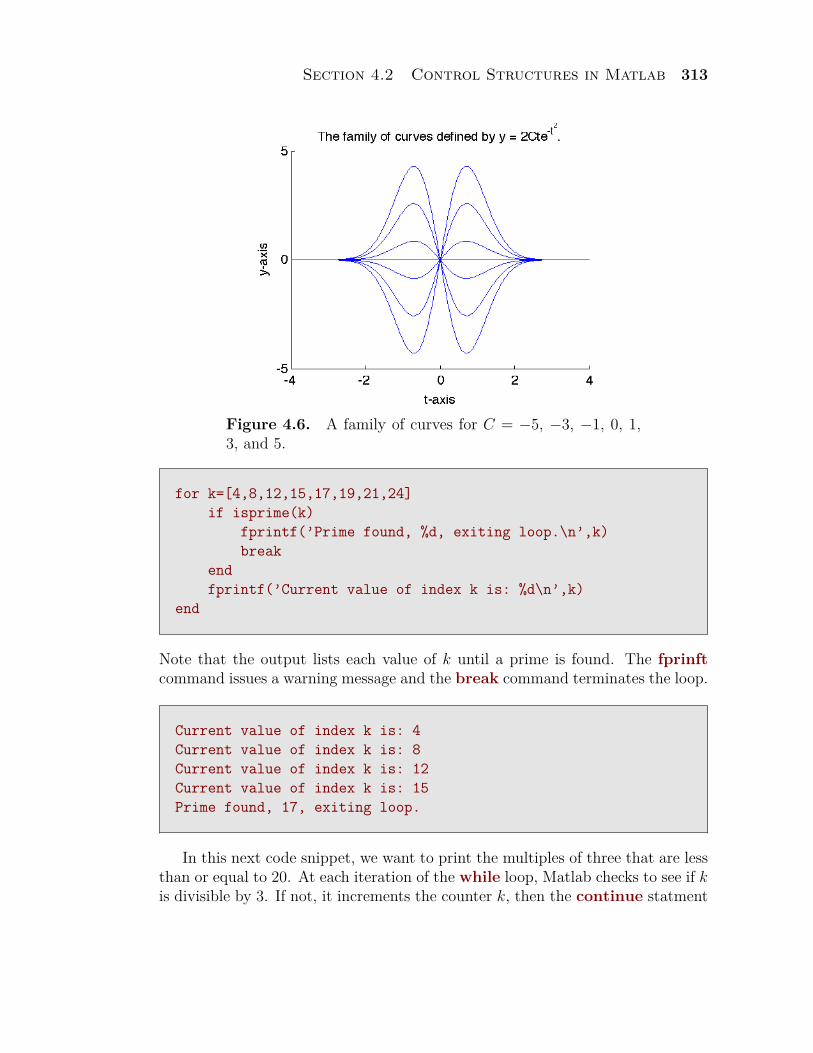
As an example of use, let’s plot the family of functions defined by the equation
y = 2Cte−t2, (4.2)
where C is one of a number of specific constants. The following code producesthe family of curves shown in Figure 4.6. At each iteration of the loop, C isassigned the next value in the row vector [-5,-3,-1,0,1,3,5].
t=linspace(-4,4,200);for C=[-5,-3,-1,0,1,3,5]
y=-2*C*t.*exp(-t.^2);line(t,y)
end
Break and ContinueThere are two sitautions that frequently occur when writing loops.
1. If a certain state is achieved, the programmer wishes to terminate the loopand pass control to the code that follows the end of the loop.
2. The programmer doesn’t want to exit the loop, but does want to pass controlto the next iteration of the loop, thereby skipping any remaining code thatremains in the loop.
As an example of the first situation, consider the following snippet of code.Matlab’s break command will cause the loop to terminate if a prime is found inthe loop index k.
Section 4.2 Control Structures in Matlab 313
Figure 4.6. A family of curves for C = −5, −3, −1, 0, 1,3, and 5.
for k=[4,8,12,15,17,19,21,24]if isprime(k)
fprintf(’Prime found, %d, exiting loop.\n’,k)break
endfprintf(’Current value of index k is: %d\n’,k)
end
Note that the output lists each value of k until a prime is found. The fprinftcommand issues a warning message and the break command terminates the loop.
Current value of index k is: 4Current value of index k is: 8Current value of index k is: 12Current value of index k is: 15Prime found, 17, exiting loop.
In this next code snippet, we want to print the multiples of three that are lessthan or equal to 20. At each iteration of the while loop, Matlab checks to see if kis divisible by 3. If not, it increments the counter k, then the continue statment
314 Chapter 4 Programming in Matlab
that follows skips the remaining statements in the loop, and returns control tothe next iteration of the loop.
N=20;k=1;while k<=N
if mod(k,3)~=0k=k+1;continue
endfprintf(’Multiple of 3: %d\n’,k)k=k+1;
end
If a multiple of 3 is found, fprintf is used to output the result in a nicely formattedstatement.
Multiple of 3: 3Multiple of 3: 6Multiple of 3: 9Multiple of 3: 12Multiple of 3: 15Multiple of 3: 18
Any and AllThe command any returns true if any element of a vector is a nonzero numberor is logical 1 (true).
>> v=[0 0 1 0 1]; any(v)ans =
1
On the other hand, any returns false if non of the elements of a vector are nonzeronumbers or logical 1’s.
Section 4.2 Control Structures in Matlab 315
>> v=[0 0 0 0]; any(v)ans =
0
The command all returns true if all of the elements of a vector are nonzeronumbers or are logical 1’s (true).
>> v=[1 1 1 1]; all(v)ans =
1
On the other hand, all returns false if the vector contains any zeros or logical0’s.
>> v=[1 0 1 1 1]; all(v)ans =
0
The any and all command can be quite useful in programs. Suppose forexample, that you want to pick out all the numbers from 1 to 2000 that aremultiples of 8, 12, and 15. Here’s a code snippet that will perform this task. Eachtime through the loop, we use the mod function to determine the remainder whenthe current value of k is divided by the numbers in divisors. If “all” remaindersare equal to zero, then k is divisible by each of the numbers in divisors and weappend k to a list of multiples of 8, 12, and 15.
N=2000;divisors=[8,12,15];multiples=[];for k=1:N
if all(mod(k,divisors)==0)multiples=[multiples,k];
endendfmt=’%5d %5d %5d %5d %5d\n’;fprintf(fmt,multiples)
316 Chapter 4 Programming in Matlab
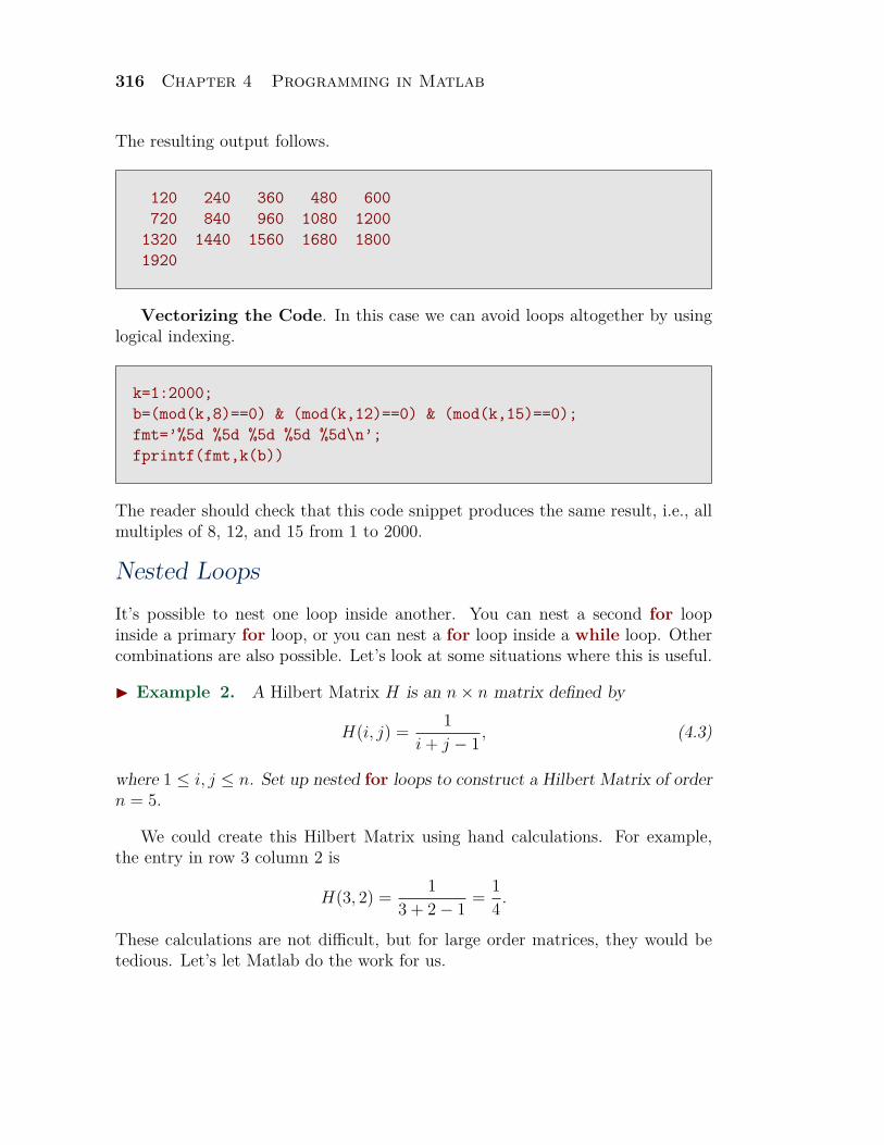
The resulting output follows.
120 240 360 480 600720 840 960 1080 1200
1320 1440 1560 1680 18001920
Vectorizing the Code. In this case we can avoid loops altogether by usinglogical indexing.
k=1:2000;b=(mod(k,8)==0) & (mod(k,12)==0) & (mod(k,15)==0);fmt=’%5d %5d %5d %5d %5d\n’;fprintf(fmt,k(b))
The reader should check that this code snippet produces the same result, i.e., allmultiples of 8, 12, and 15 from 1 to 2000.
Nested LoopsIt’s possible to nest one loop inside another. You can nest a second for loopinside a primary for loop, or you can nest a for loop inside a while loop. Othercombinations are also possible. Let’s look at some situations where this is useful.
I Example 2. A Hilbert Matrix H is an n× n matrix defined by
H(i, j) = 1i + j − 1
, (4.3)
where 1 ≤ i, j ≤ n. Set up nested for loops to construct a Hilbert Matrix of ordern = 5.
We could create this Hilbert Matrix using hand calculations. For example,the entry in row 3 column 2 is
H(3, 2) = 13 + 2− 1
= 14.
These calculations are not difficult, but for large order matrices, they would betedious. Let’s let Matlab do the work for us.

Section 4.2 Control Structures in Matlab 317
n=5;H=zeros(n);
Now, doubly nested for loops achieve the desired result.
for i=1:nfor j=1:n
H(i,j)=1/(i+j-1);end
end
Set rational display format, display the matrix H, then set the format back todefault.
format ratHformat
The result is shown in the following Hilbert Matrix of order 5.
H =1 1/2 1/3 1/4 1/51/2 1/3 1/4 1/5 1/61/3 1/4 1/5 1/6 1/71/4 1/5 1/6 1/7 1/81/5 1/6 1/7 1/8 1/9
Note that the entry is row 3 column 2 is 1/4, as predicted by our hand calculationsabove. Similar hand calculations can be used to verify other entries in this result.
How does it work? Because n = 5, the primary loop becomes for i=1:5.Similarly, the inner loop becomes for j=1:5. Now, here is the way the nestedstructure proceeds. First, set i = 1, then execute the statement H(i,j)=1/(i+j-1) for j = 1, 2, 3, 4, and 5. With this first pass, we set the entries H(1, 1), H(1, 2),H(1, 3), H(1, 4), and H(1, 5). The inner loop terminates and control returns tothe primary loop, where the program next sets i = 2 and again executes thestatement H(i,j)=1/(i+j-1) for j = 1, 2, 3, 4, and 5. With this second pass, weset the entries H(2, 1), H(2, 2), H(2, 3), H(2, 4), and H(2, 5). A third and fourth
318 Chapter 4 Programming in Matlab
pass of the primary loop occur next, with i = 3 and 4, each time iterating theinner loop for j = 1, 2, 3, 4, and 5. Finally, on the last pass through the primary,the program sets i = 5, then executes the statement H(i,j)=1/(i+j-1) for j = 1,2, 3, 4, and 5. On this last pass, the program sets the entries H(5, 1), H(5, 2),H(5, 3), H(5, 4), and H(5, 5) and terminates.
Fourier Series — An Application of a For LoopMatlab’s mod(a,b) works equally well with real numbers, providing the remain-der when a is divided by b. For example, if you divide 5.7 by 2, the quotientis 2 and the remainder is 1.7. The command mod(5.7,2) should return theremainder, namely 1.7.
>> mod(5.7,2)ans =
1.7000
The following commands produce what engineers call a sawtooth curve, shown inFigure 4.7(a).
t=linspace(0,6,500);y=mod(t,2);plot(t,y)
In Figure 4.7(a), we plot the remainders when the time is divided by 2. Hence,we get the a periodic function of period 2, where the remainders grow from 0 tojust less than 2, then repeat every 2 units.
With the following adjustment, we produce what engineers call a square wave(shown in Figure 4.7(b)). Recall that y<1 returns true (logical 1) when y isless than 1, and false (logical 0) when y is not less than 1.
y=(y<1);plot(t,y,’*’)
This type of curve can emulate a switch that is “on” for one second (y-value 1),then off for the next second (y-value 0), and then periodically repeats this “on-off”cycle over its domain.
Section 4.2 Control Structures in Matlab 319
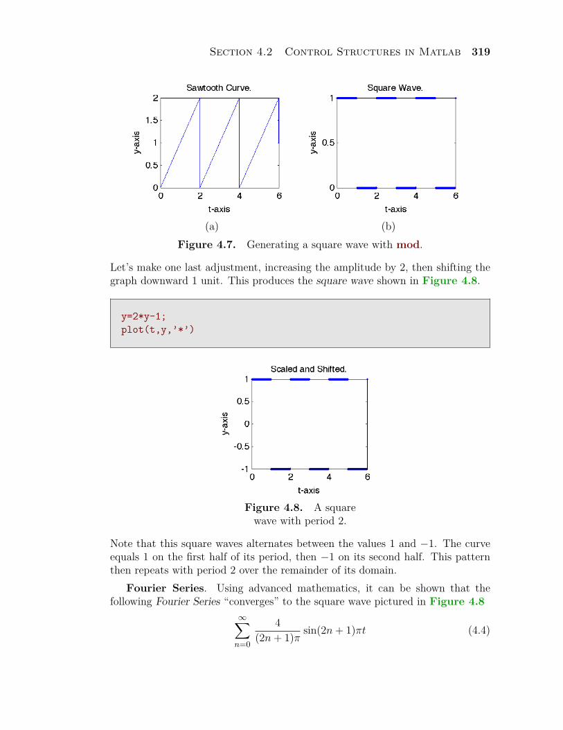
(a) (b)Figure 4.7. Generating a square wave with mod.
Let’s make one last adjustment, increasing the amplitude by 2, then shifting thegraph downward 1 unit. This produces the square wave shown in Figure 4.8.
y=2*y-1;plot(t,y,’*’)
Figure 4.8. A squarewave with period 2.
Note that this square waves alternates between the values 1 and −1. The curveequals 1 on the first half of its period, then −1 on its second half. This patternthen repeats with period 2 over the remainder of its domain.
Fourier Series. Using advanced mathematics, it can be shown that thefollowing Fourier Series “converges” to the square wave pictured in Figure 4.8
∞∑n=0
4(2n + 1)π
sin(2n + 1)πt (4.4)
320 Chapter 4 Programming in Matlab
It is certainly remarkable, if not somewhat implausible, that one can sum a seriesof sinusoidal function and get the resulting square wave picture in Figure 4.8.
We will generate and plot the first five terms of the series (4.4), saving eachterm in a row of matrix A for later use. First, we initialize the time and thenumber of terms of the series that we will use, then we allocate appropriate spacefor matrix A. Note how we wisely save the number of points and the number ofterms in variables, so that if we later decide to change these values, we won’t haveto scan every line of our program making changes.
N=500;numterms=5;t=linspace(0,6,N);A=zeros(numterms,N);
Next, we use a for loop to compute each of the first 5 terms (numterms) ofseries (4.4), storing each term in a row of matrix A, then plotting the sinusoid inthree space, where we use the angular frequency as the third dimension.
for n=0:numterms-1y=4/((2*n+1)*pi)*sin((2*n+1)*pi*t);A(n+1,:)=y;line((2*n+1)*pi*ones(size(t)),t,y)
end
We orient the 3D-view, add a box for depth, turn on the grid, and annotate eachaxis to produce the image shown in Figure 4.9(a).
view(20,20)box ongrid onxlabel(’Angular Frequency’)ylabel(’t-axis’)zlabel(’y-axis’)
As one would expect, after examining the terms of series (4.4), each each consecu-tive term of the series is a sinusoid with increasing angular frequency and decreas-ing amplitude. This is evident with the sequence of terms shown in Figure 4.9(a).
Section 4.2 Control Structures in Matlab 321
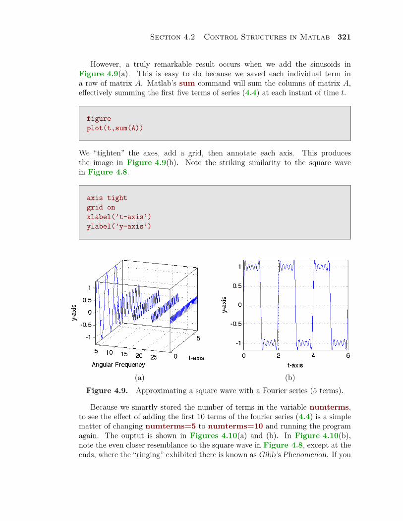
However, a truly remarkable result occurs when we add the sinusoids inFigure 4.9(a). This is easy to do because we saved each individual term ina row of matrix A. Matlab’s sum command will sum the columns of matrix A,effectively summing the first five terms of series (4.4) at each instant of time t.
figureplot(t,sum(A))
We “tighten” the axes, add a grid, then annotate each axis. This producesthe image in Figure 4.9(b). Note the striking similarity to the square wavein Figure 4.8.
axis tightgrid onxlabel(’t-axis’)ylabel(’y-axis’)
(a) (b)Figure 4.9. Approximating a square wave with a Fourier series (5 terms).
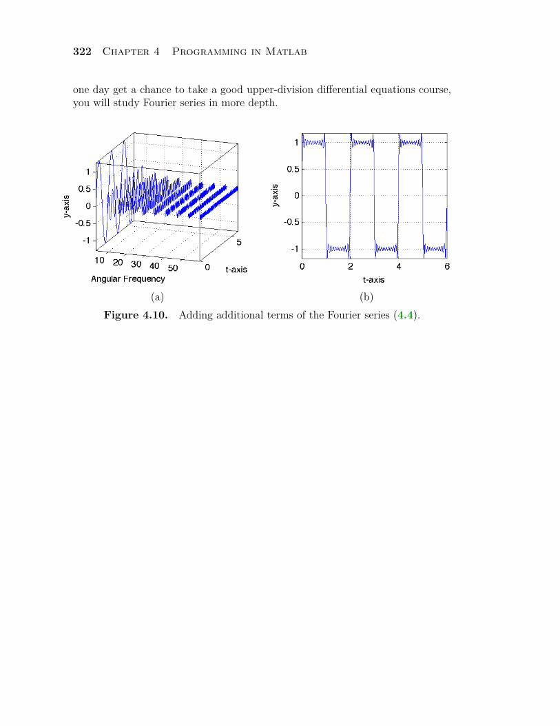
Because we smartly stored the number of terms in the variable numterms,to see the effect of adding the first 10 terms of the fourier series (4.4) is a simplematter of changing numterms=5 to numterms=10 and running the programagain. The ouptut is shown in Figures 4.10(a) and (b). In Figure 4.10(b),note the even closer resemblance to the square wave in Figure 4.8, except at theends, where the “ringing” exhibited there is known as Gibb’s Phenomenon. If you
322 Chapter 4 Programming in Matlab
one day get a chance to take a good upper-division differential equations course,you will study Fourier series in more depth.
(a) (b)Figure 4.10. Adding additional terms of the Fourier series (4.4).
Section 4.2 Control Structures in Matlab 323
4.2 Exercises
1. Write a for loop that will out-put the cubes of the first 10 positiveintegers. Use fprintf to output the re-sults, which should include the integerand its cube. Write a second programthat uses a while loop to produce anindentical result.
2. Without appealing to the Matlabcommand factorial, write a for loopto output the factorial of the numbers10 through 15. Use fprintf to formatthe output. Write a second programthat uses a while loop to produce anindentical result. Hint: Consider theprod command.
3. Write a single program that willcount the number of divisors of each ofthe following integers: 20, 36, 84, and96. Use fprintf to output each resultin a form similar to “The number ofdivisors of 12 is 6.”
4. Set A=magic(5). Write a pro-gram that uses nested for loops tofind the sum of the squares of all en-tries of matrix A. Use fprintf to for-mat the output. Write a second pro-gram that uses array operations andMatlab’s sum function to obtain thesame result.
5. Write a program that uses nestedfor loops to produce Pythagorean Triples,positive integers a, b and c that satisfya2+b2 = c2. Find all such triples suchthat 1 ≤ a, b, c ≤ 20 and use fprintf
Copyrighted material. See: http://msenux.redwoods.edu/IntAlgText/6
to produce nicely formatted results.
6. Another result proved by Leon-hard Euler shows that
π4
90= 1 + 1
24 + 134 + 1
44 + · · · .
Write a program that uses a for loopto sum the first 20 terms of this series.Compute the relative error when thissum is used as an approximation ofπ4/90. Write a second program thatuses a while loop to determine thenumber of terms required so that thesum approximates π4/90 to four sig-nificant digits. In both programs, usefprintf to format your output.
7. Some attribute the following se-ries to Leibniz.
π
4= 1− 1
3+ 1
5− 1
7+ 1
9− · · ·
Write a program that uses a for loopto sum the first 20 terms of this se-ries. Compute the relative error whenthis sum is used as an approximationof π/4. Write a second program thatuses a while loop to determine thenumber of terms required so that thesum approximates π/4 to four signif-icant digits. In both programs, usefprintf to format your output.
8. Goldbach’s Conjecture is one ofthe most famous unproved conjecturesin all of mathematics, which is remark-able in light of its simplistic statement:
324 Chapter 4 Programming in Matlab
All even integers greater than2 can be expressed as a sum oftwo prime integers.
Write a program that expresses 1202as the sum of two primes in ten differ-ent ways. Use fprintf to format youroutput.
9. Here is a simple idea for gener-ating a list of prime integers. Createa vector primes with a single entry,the prime integer 2. Write a programto test each integer less than 100 tosee if it is a prime using the followingprocedure.
i. If an integer is divisible by any ofthe integers in primes, skip it andgo to the next integer.
ii. If an integer is not divisible by anyof the integers in primes, appendthe integer to the vector primesand go to the next integer.
Use fprintf to output the vector primesin five columns, right justified.
10. There is a famous stoy about SirThomas Hardy and Srinivasa Ramanu-jan, which Hardy relates in his famouswork “A Mathematician’s Apology,”a copy of which resides in the CR li-brary along with the work “The ManWho Knew Infinity: A Life of the Ge-nius Ramanujan.”
I remember once going to seehim when he was ill at Putney.I had ridden in taxi cab num-ber 1729 and remarked that thenumber seemed to me rather adull one, and that I hoped itwas not an unfavorable omen.“No,” he replied, “it is a very
interesting number; it is the small-est number expressible as thesum of two cubes in two differ-ent ways.”
Write a program with nested loops tofind integers a and b (in two ways) sothat a3 + b3 = 1729. Use fprintf toformat the output of your program.
11. Write a program to perform eachof the following tasks.
i. Use Matlab to draw a circle of ra-dius 1 centered at the origin andinscribed in a square having ver-tices (1, 1), (−1, 1), (−1,−1), and(1,−1). The ratio of the area ofthe circle to the area of the squareis π : 4 or π/4. Hence, if we wereto throw darts at the square in arondom fashion, the ratio of dartsinside the circle to the number ofdarts thrown should be approxi-mately equal to π/4.
ii. Write a for loop that will plot 1000randomly generated points insidethe square. Use Matlab’s randcommand for this task. Each timerandom point lands within the unitcircle, increment a counter hits.When the for loop terminates, usefprintf to output the ratio dartsthat land inside the circle to thenumber of darts thrown. Calcu-late the relative error in approxi-mating π/4 with this ratio.
12. Write a program to perform eachof the following tasks.
i. Prompt the user to enter a 3 × 4matrix. Store the result in the ma-trix A.
Section 4.2 Control Structures in Matlab 325
ii. Use if..elseif..else to provide a menuwith three choices: (1) Switch tworows of the matrix; (2) Multiply arow of the matrix by a scalar; and(3) Subtract a scalar multiple of arow from another row of the ma-trix.
iii. Perform the task in the requestedmenu item, then return the result-ing matrix to the user.a. In the case of (1), your pro-
gram should prompt the userfor the rows to switch.
b. In the case of (2), your pro-gram should prompt the userfor a scalar and a row that willbe multiplied by the scalar.
c. In the case of (3), your pro-gram should prompt the userfor a scalar and two row num-bers, the first of which is tobe multiplied by the scalar andsubtracted from the second.
13. The solutions of the quadraticequation ax2 +bx+c = 0 are given bythe quadratic formula
x = −b±√
b2 − 4ac
2a.
The discriminant D = b2−4ac is usedto predict the number of roots. Thereare three cases.
1. If D > 0, there are two real solu-tions.
2. If D = 0, there is one real solution.3. If D < 0, there are no real solu-
tions.
Write a program the performs each ofthe following tasks.
i. The program prompts the user to
input a, b, and c.ii. The programs computes the dis-
criminant D which it uses with theconditional if..elseif..else to de-termine and output the number ofsolutions.
iii. The program should also outputthe solutions, if any.
Use well crafted format strings withfprintf to output all results.
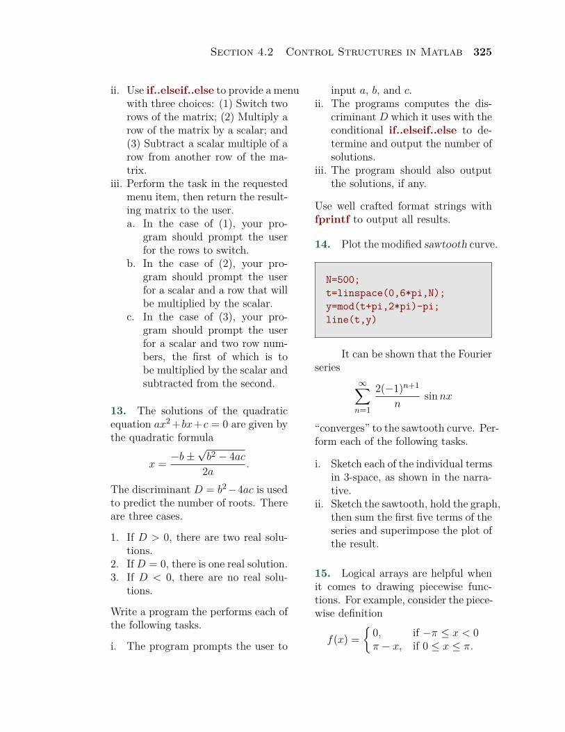
14. Plot the modified sawtooth curve.
N=500;t=linspace(0,6*pi,N);y=mod(t+pi,2*pi)-pi;line(t,y)
It can be shown that the Fourierseries
∞∑n=1
2(−1)n+1
nsin nx
“converges” to the sawtooth curve. Per-form each of the following tasks.
i. Sketch each of the individual termsin 3-space, as shown in the narra-tive.
ii. Sketch the sawtooth, hold the graph,then sum the first five terms of theseries and superimpose the plot ofthe result.
15. Logical arrays are helpful whenit comes to drawing piecewise func-tions. For example, consider the piece-wise definition
f(x) ={
0, if −π ≤ x < 0π − x, if 0 ≤ x ≤ π.
326 Chapter 4 Programming in Matlab
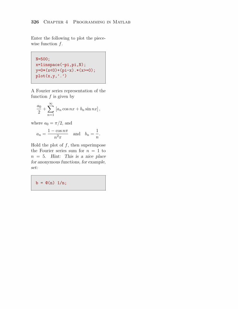
Enter the following to plot the piece-wise function f .
N=500;x=linspace(-pi,pi,N);y=0*(x<0)+(pi-x).*(x>=0);plot(x,y,’.’)
A Fourier series representation of thefunction f is given by
a02
+∞∑
n=1[an cos nx + bn sin nx] ,
where a0 = π/2, and
an = 1− cos nπ
n2πand bn = 1
n.
Hold the plot of f , then superimposethe Fourier series sum for n = 1 ton = 5. Hint: This is a nice placefor anonymous functions, for example,set:
b = @(n) 1/n;
Section 4.2 Control Structures in Matlab 327
4.2 Answers
1. This for loop will print the cubes of the first 10 positive integers.
for k=1:10fprintf(’The cube of %d is %d.\n’,k,k^3)
end
This while loop will print the cubes of the first 10 positive integers.
k=1;while k<=10
fprintf(’The cube of %d is %d.\n’,k,k^3)k=k+1;
end
3. The following program will print the number of divisors of 20, 36, 84, and 96.
for k=[20, 36, 84, 96]count=0;divisor=1;while (divisor<=k)
if mod(k,divisor)==0count=count+1;
enddivisor=divisor+1;
endfprintf(’The number of divisors of %d is %d.\n’,k,count)
end
5. This program will print Pythagorean Triples so that 1 ≤ a, b, c ≤ 20.
328 Chapter 4 Programming in Matlab
N=20;for a=1:N
for b=1:Nfor c=1:N
if (c^2==a^2+b^2)fprintf(’Pythagorean Triple: %d, %d, %d\n’, a, b, c)
endend
endend
7. The following loop will sum the first 20 terms.
N=20;s=0;for k=1:N;
s=s+(-1)^(k+1)/(2*k-1);end
Compute the relative error in approximating π/4 with the sum of the first 20terms.
rel=abs(s-pi/4)/abs(pi/4);
Output the results.
fprintf(’The actual value of pi/4 is %.6f.\n’,pi/4)fprintf(’The sum of the first %d terms is %f.\n’,N,s)fprintf(’The relative error is %.2e.\n’,rel)
9. The mod(m,primes)==0 comparison will produce a logical vector whichcontains a 1 in each position that indicates that the current number m is divisibleby the number in the prime vector in the corresponding position. If “any” ofthese are 1’s, then the number m is divisible by at least one of the primes in thecurrent list primes. In that case, we continue to the next value of m. Otherwise,we append m to the list of primes.
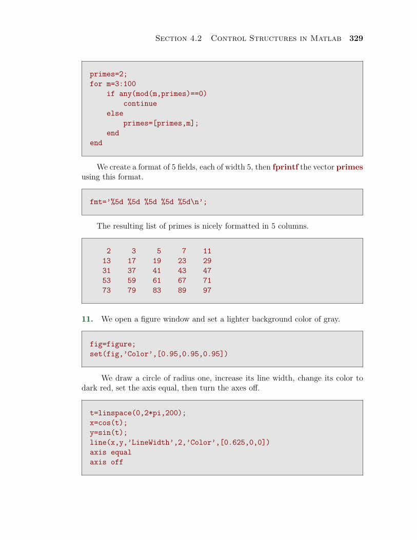
Section 4.2 Control Structures in Matlab 329
primes=2;for m=3:100
if any(mod(m,primes)==0)continue
elseprimes=[primes,m];
endend
We create a format of 5 fields, each of width 5, then fprintf the vector primesusing this format.
fmt=’%5d %5d %5d %5d %5d\n’;
The resulting list of primes is nicely formatted in 5 columns.
2 3 5 7 1113 17 19 23 2931 37 41 43 4753 59 61 67 7173 79 83 89 97
11. We open a figure window and set a lighter background color of gray.
fig=figure;set(fig,’Color’,[0.95,0.95,0.95])
We draw a circle of radius one, increase its line width, change its color todark red, set the axis equal, then turn the axes off.
t=linspace(0,2*pi,200);x=cos(t);y=sin(t);line(x,y,’LineWidth’,2,’Color’,[0.625,0,0])axis equalaxis off
330 Chapter 4 Programming in Matlab
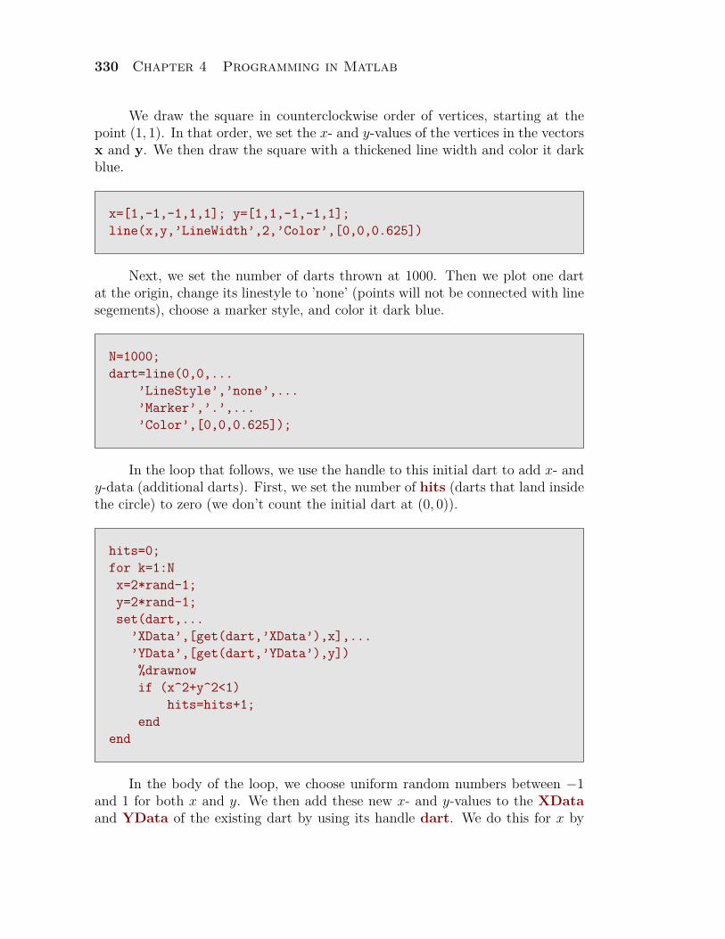
We draw the square in counterclockwise order of vertices, starting at thepoint (1, 1). In that order, we set the x- and y-values of the vertices in the vectorsx and y. We then draw the square with a thickened line width and color it darkblue.
x=[1,-1,-1,1,1]; y=[1,1,-1,-1,1];line(x,y,’LineWidth’,2,’Color’,[0,0,0.625])
Next, we set the number of darts thrown at 1000. Then we plot one dartat the origin, change its linestyle to ’none’ (points will not be connected with linesegements), choose a marker style, and color it dark blue.
N=1000;dart=line(0,0,...
’LineStyle’,’none’,...’Marker’,’.’,...’Color’,[0,0,0.625]);
In the loop that follows, we use the handle to this initial dart to add x- andy-data (additional darts). First, we set the number of hits (darts that land insidethe circle) to zero (we don’t count the initial dart at (0, 0)).
hits=0;for k=1:Nx=2*rand-1;y=2*rand-1;set(dart,...
’XData’,[get(dart,’XData’),x],...’YData’,[get(dart,’YData’),y])%drawnowif (x^2+y^2<1)
hits=hits+1;end
end
In the body of the loop, we choose uniform random numbers between −1and 1 for both x and y. We then add these new x- and y-values to the XDataand YData of the existing dart by using its handle dart. We do this for x by
Section 4.2 Control Structures in Matlab 331
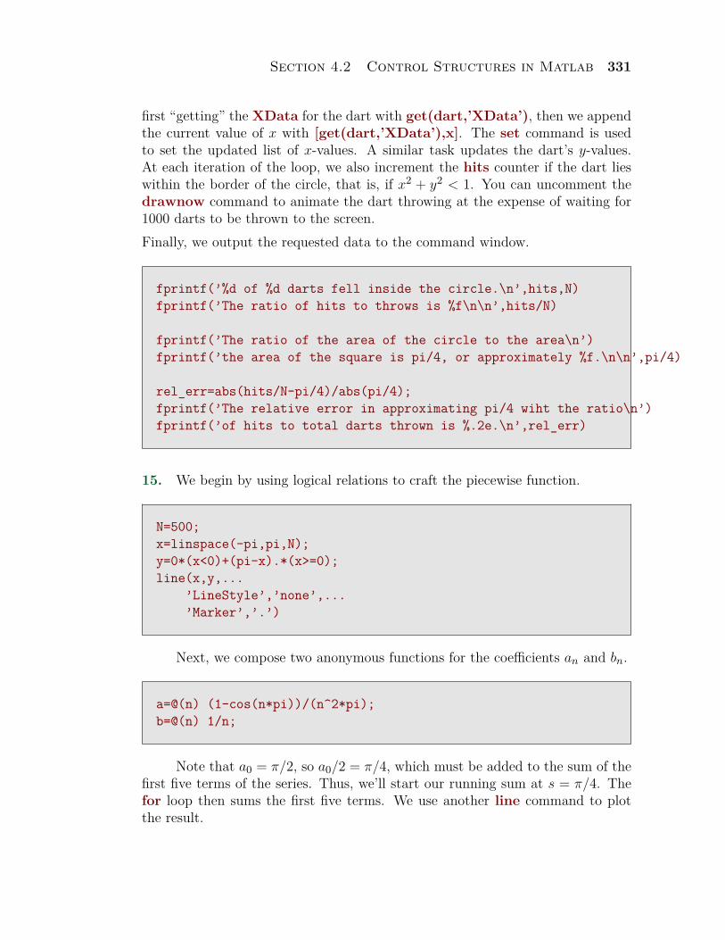
first “getting” the XData for the dart with get(dart,’XData’), then we appendthe current value of x with [get(dart,’XData’),x]. The set command is usedto set the updated list of x-values. A similar task updates the dart’s y-values.At each iteration of the loop, we also increment the hits counter if the dart lieswithin the border of the circle, that is, if x2 + y2 < 1. You can uncomment thedrawnow command to animate the dart throwing at the expense of waiting for1000 darts to be thrown to the screen.Finally, we output the requested data to the command window.
fprintf(’%d of %d darts fell inside the circle.\n’,hits,N)fprintf(’The ratio of hits to throws is %f\n\n’,hits/N)
fprintf(’The ratio of the area of the circle to the area\n’)fprintf(’the area of the square is pi/4, or approximately %f.\n\n’,pi/4)
rel_err=abs(hits/N-pi/4)/abs(pi/4);fprintf(’The relative error in approximating pi/4 wiht the ratio\n’)fprintf(’of hits to total darts thrown is %.2e.\n’,rel_err)
15. We begin by using logical relations to craft the piecewise function.
N=500;x=linspace(-pi,pi,N);y=0*(x<0)+(pi-x).*(x>=0);line(x,y,...
’LineStyle’,’none’,...’Marker’,’.’)
Next, we compose two anonymous functions for the coefficients an and bn.
a=@(n) (1-cos(n*pi))/(n^2*pi);b=@(n) 1/n;
Note that a0 = π/2, so a0/2 = π/4, which must be added to the sum of thefirst five terms of the series. Thus, we’ll start our running sum at s = π/4. Thefor loop then sums the first five terms. We use another line command to plotthe result.
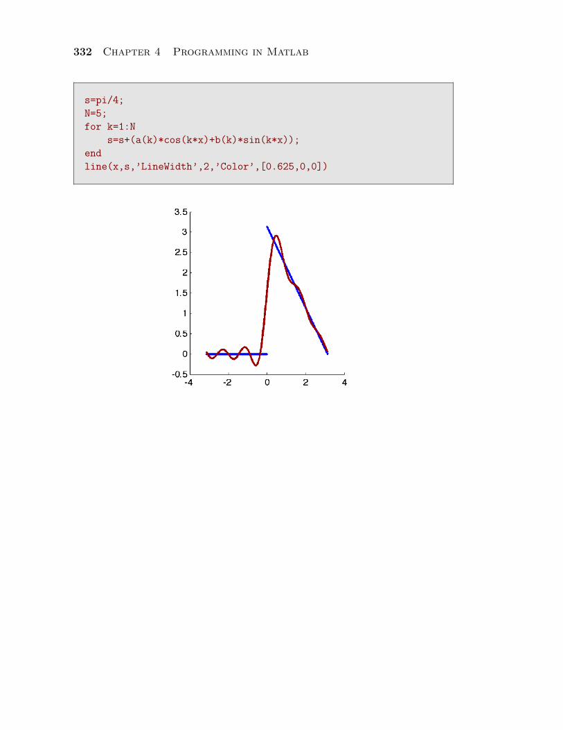
332 Chapter 4 Programming in Matlab
s=pi/4;N=5;for k=1:N
s=s+(a(k)*cos(k*x)+b(k)*sin(k*x));endline(x,s,’LineWidth’,2,’Color’,[0.625,0,0])
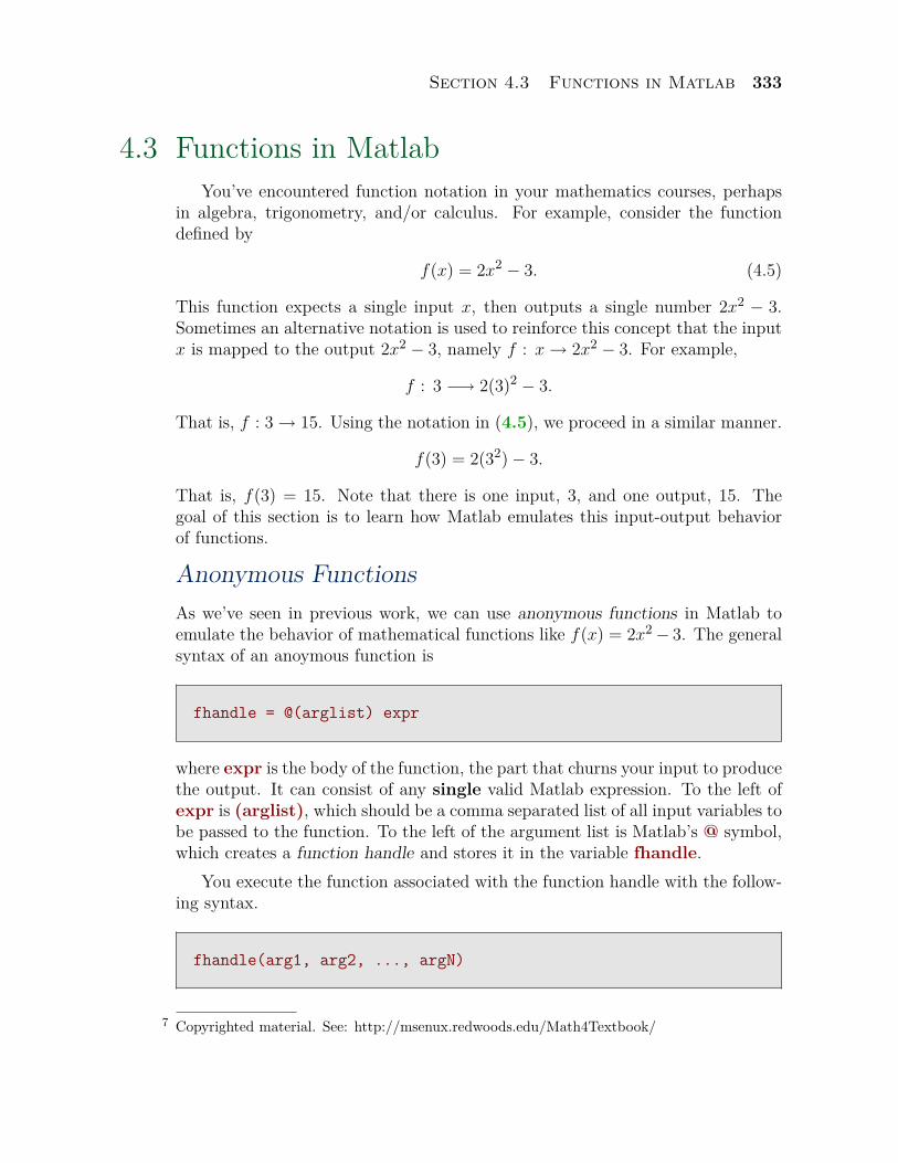
Section 4.3 Functions in Matlab 333
4.3 Functions in MatlabYou’ve encountered function notation in your mathematics courses, perhaps
in algebra, trigonometry, and/or calculus. For example, consider the functiondefined by
f(x) = 2x2 − 3. (4.5)
This function expects a single input x, then outputs a single number 2x2 − 3.Sometimes an alternative notation is used to reinforce this concept that the inputx is mapped to the output 2x2 − 3, namely f : x → 2x2 − 3. For example,
f : 3 −→ 2(3)2 − 3.
That is, f : 3 → 15. Using the notation in (4.5), we proceed in a similar manner.
f(3) = 2(32)− 3.
That is, f(3) = 15. Note that there is one input, 3, and one output, 15. Thegoal of this section is to learn how Matlab emulates this input-output behaviorof functions.
Anonymous FunctionsAs we’ve seen in previous work, we can use anonymous functions in Matlab toemulate the behavior of mathematical functions like f(x) = 2x2− 3. The generalsyntax of an anoymous function is
fhandle = @(arglist) expr
where expr is the body of the function, the part that churns your input to producethe output. It can consist of any single valid Matlab expression. To the left ofexpr is (arglist), which should be a comma separated list of all input variables tobe passed to the function. To the left of the argument list is Matlab’s @ symbol,which creates a function handle and stores it in the variable fhandle.
You execute the function associated with the function handle with the follow-ing syntax.
fhandle(arg1, arg2, ..., argN)
Copyrighted material. See: http://msenux.redwoods.edu/Math4Textbook/7
334 Chapter 4 Programming in Matlab
That is, you specify the variable holding the function handle, followed by a commaseparated list of arguments in parentheses.
I Example 1. Create a function to emulate the behavior of the mathematicalfunction f(x) = 2x2 − 3.
We use the syntax fhandle = @(arglist) expr to create and store a functionhandle in the variable f .
>> f = @(x) 2*x^2 - 3f =
@(x) 2*x^2 - 3
We now execute the function by specifying the function handle associated withit, followed by a single argument (the input) in parentheses.
>> f(3)ans =
15
However, note what happens when we pass an array as input to this function.
>> x=0:5x =
0 1 2 3 4 5>> f(x)??? Error using ==> mpowerMatrix must be square.
Error in ==> @(x) 2*x^2 - 3
We’ve failed to make our function “array smart.” You cannot square a vector, aswe are reminded in the error message “Matrix must be square.” We need to usearray operators to make our anonymous function “array smart.”
>> f = @(x) 2*x.^2 -3f =
@(x) 2*x.^2 -3
Section 4.3 Functions in Matlab 335
Note that this time we used the “dot raised to” operator .^ which will operateelementwise and square each entry of the input. Note that using an array as inputis now successful, and the function is evaluated at each entry of the input vectorx=0:5.
>> f(x)ans =
-3 -1 5 15 29 47
Even though we’ve made our function array smart, it will still operate on indi-vidual scalar entries.
>> f(5)ans =
47
Making Functions Array Smart. Many of Matlab’s routines require thata function passed as an argument be “array smart.” You need to be awareof this if you pass a function to one of these routines.
Let’s look at another example.
I Example 2. Create a function to emulate the mathematical behavior of thefunction defined by f(x, y) = 9− x2 − y2.
Note that there are two inputs to the function f . As an example, we evaluatethe function at the point (x, y) = (2, 3).
f(2, 3) = 9− 22 − 32.
Thus, f(2, 3) = −4.We define an anonymous Matlab function to emulate the behavior of f . Note
that the the @ symbol is followed by a comma delimited list of two variables xand y, contained in parentheses.
336 Chapter 4 Programming in Matlab
>> f= @(x,y) 9 - x^2 - y^2f =
@(x,y) 9 - x^2 - y^2
We evaluate the function f at (x, y) = (2, 3) as follows.
>> f(2,3)ans =
-4
Note that this agrees with our hand calculation above.
It’s possible to use constants in your anonymous function that are previouslydefined in your current workspace.
I Example 3. Write a function to evaluate f(x, y, z) = Ax + By + Cz at thepoint (−1, 2,−3), where A = 2, B = 3, and C = −4 are previously defined in thecurrent workspace.
Set the constants A = 2, B = 3, and C = −4.
>> A=2; B=3; C=-4;
Now, define the anonymous function as follows.
>> f = @(x,y,z) A*x + B*y + C*zf =
@(x,y,z) A*x + B*y + C*z
Now, evaluating the function at (x, y, z) = (−1, 2,−3) by hand,
f(−1, 2,−3) = A(−1) + B(2) + C(−3) = (2)(−1) + (3)(2) + (−4)(−3) = 16.
Checking in Matlab.
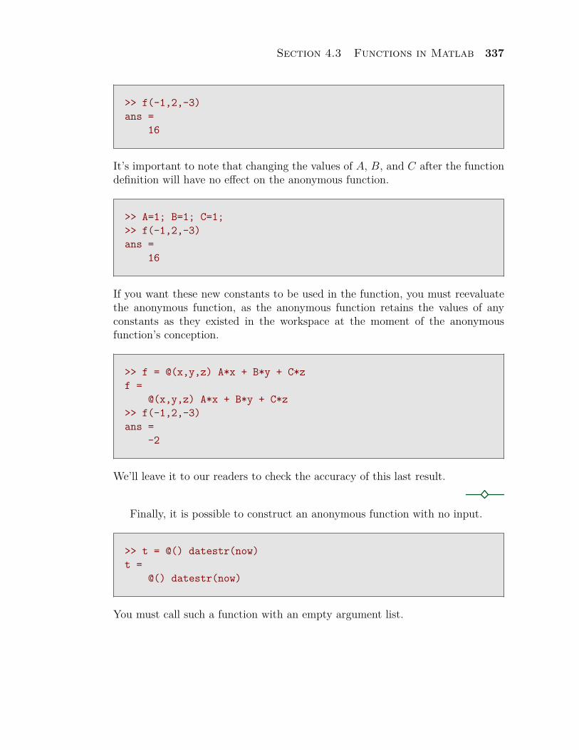
Section 4.3 Functions in Matlab 337
>> f(-1,2,-3)ans =
16
It’s important to note that changing the values of A, B, and C after the functiondefinition will have no effect on the anonymous function.
>> A=1; B=1; C=1;>> f(-1,2,-3)ans =
16
If you want these new constants to be used in the function, you must reevaluatethe anonymous function, as the anonymous function retains the values of anyconstants as they existed in the workspace at the moment of the anonymousfunction’s conception.
>> f = @(x,y,z) A*x + B*y + C*zf =
@(x,y,z) A*x + B*y + C*z>> f(-1,2,-3)ans =
-2
We’ll leave it to our readers to check the accuracy of this last result.
Finally, it is possible to construct an anonymous function with no input.
>> t = @() datestr(now)t =
@() datestr(now)
You must call such a function with an empty argument list.
338 Chapter 4 Programming in Matlab
>> t()ans =04-Mar-2007 00:34:07
Function M-FilesNote that the anonymous function syntax fhandle = @(args) expr only allowsfor a single Matlab expression in its definition body. Moreover, only one outputvariable is allowed. In this section we will look at Function M-files, which aresimilar to scripts, but allow for both multiple input and output and as many linesas needed in the body of the function.
Like script files, you write function m-files in the Matlab editor. The first lineof the function m-file must contain the following syntax.
function [out1, out2, ...] = funname(in1, in2, ...)
The keyword function must be the first word in the function m-file. This alertsthe Matlab interpreter that the file contains a function, not a script. Next comesa comma delimited list of output arguments (surrounding brackets are requiredif more than one output variable is used), then an equal sign, followed by thefunction name. The function name funname must be string composed of letters,digits, and underscores. The first character of the name must be a letter. Avalid length for the function name varies from machine to machine, but can bedetermined by the command namelengthmax.
>> namelengthmaxans =
63
If you name your function funname, as above, you must save the function m-fileas funname.m. That is, you must attach .m to the function name when savingthe function m-file.
After the function name comes a comma delimited list of input variables,surrounded by required parentheses. Input arguments are passed by value and allvariables in the body of the function are “local” to the function (we’ll have moreto say about local and global variables later). In the body of the function m-file,
Section 4.3 Functions in Matlab 339
you must assign a value to each output variable before the function definition iscomplete.
Before getting too ambitious, let’s start with some simple examples of functionM-files that emulate the behavior of the anonymous functions in Examples 1through 3.
I Example 4. Write a function m-file to emulate the behavior of the functionf(x) = 2x2 − 3.
Open the Matlab editor and enter the following lines.
function y=f(x)y=2*x^2-3;
Note how we’ve followed the syntax rules outlined above.
i. The first word on the first line is the keyword function.ii. We are using y as the output variable. Because there is only a single output
variable, the surrounding brackets are not required.iii. The function name is f.iv. Finally, surrounded in required parentheses is a single input variable x.
Save the file as f.m. Note how we’ve attached .m to the function name f.In Example 1, we found that f(3) = 15. Let’s test the current function.
Return to the command window and enter the following at the Matlab prompt.
>> f(3)ans =
15
As in Example 1, the current function is not “array smart,” so attempting toevaluate the function on an array will fail.
340 Chapter 4 Programming in Matlab
>> x=0:5x =
0 1 2 3 4 5>> f(x)??? Error using ==> mpowerMatrix must be square.
Error in ==> f at 2y=2*x^2-3;
Return to the editor and make the following change to the functon m-file.
function y=f(x)y=2*x.^2-3;
Note that we have replaced the regular exponentiation symbol ^ with the ar-ray exponentiation symbol .^ (“dot raised to”). This makes our function “arraysmart” and we can now evaluate the function at each entry of the vector x.
>> f(x)ans =
-3 -1 5 15 29 47
In the next example, we use a function m-file to emulate the behavior inExample 2.
I Example 5. Write a function m-file for f(x, y) = 9− x2 − y2. Evaluate thefunction at (x, y) = (2, 3).
Open the Matlab editor and enter the following lines.
function z=f(x,y)z=9-x^2-y^2;
Note that this time we have two input variables, x and y. The function name isf, so we again save the file as f.m. Evaluate the function at (x, y) = (2, 3) at theMatlab prompt in the command window.
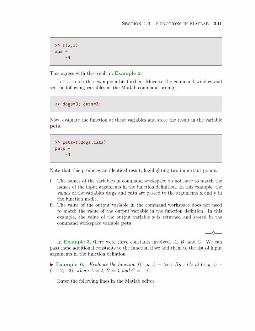
Section 4.3 Functions in Matlab 341
>> f(2,3)ans =
-4
This agrees with the result in Example 2.Let’s stretch this example a bit further. Move to the command window and
set the following variables at the Matlab command prompt.
>> dogs=3; cats=3;
Now, evaluate the function at these variables and store the result in the variablepets.
>> pets=f(dogs,cats)pets =
-4
Note that this produces an identical result, highlighting two important points.
i. The names of the variables in command workspace do not have to match thenames of the input arguments in the function definition. In this example, thevalues of the variables dogs and cats are passed to the arguments x and y inthe function m-file.
ii. The value of the output variable in the command workspace does not needto match the value of the output variable in the function defintion. In thisexample, the value of the output variable z is returned and stored in thecommand workspace variable pets.
In Example 3, there were three constants involved, A, B, and C. We canpass these additional constants to the function if we add them to the list of inputarguments in the function defintion.
I Example 6. Evaluate the function f(x, y, z) = Ax + By + Cz at (x, y, z) =(−1, 2,−3), where A = 2, B = 3, and C = −4.
Enter the following lines in the Matlab editor.
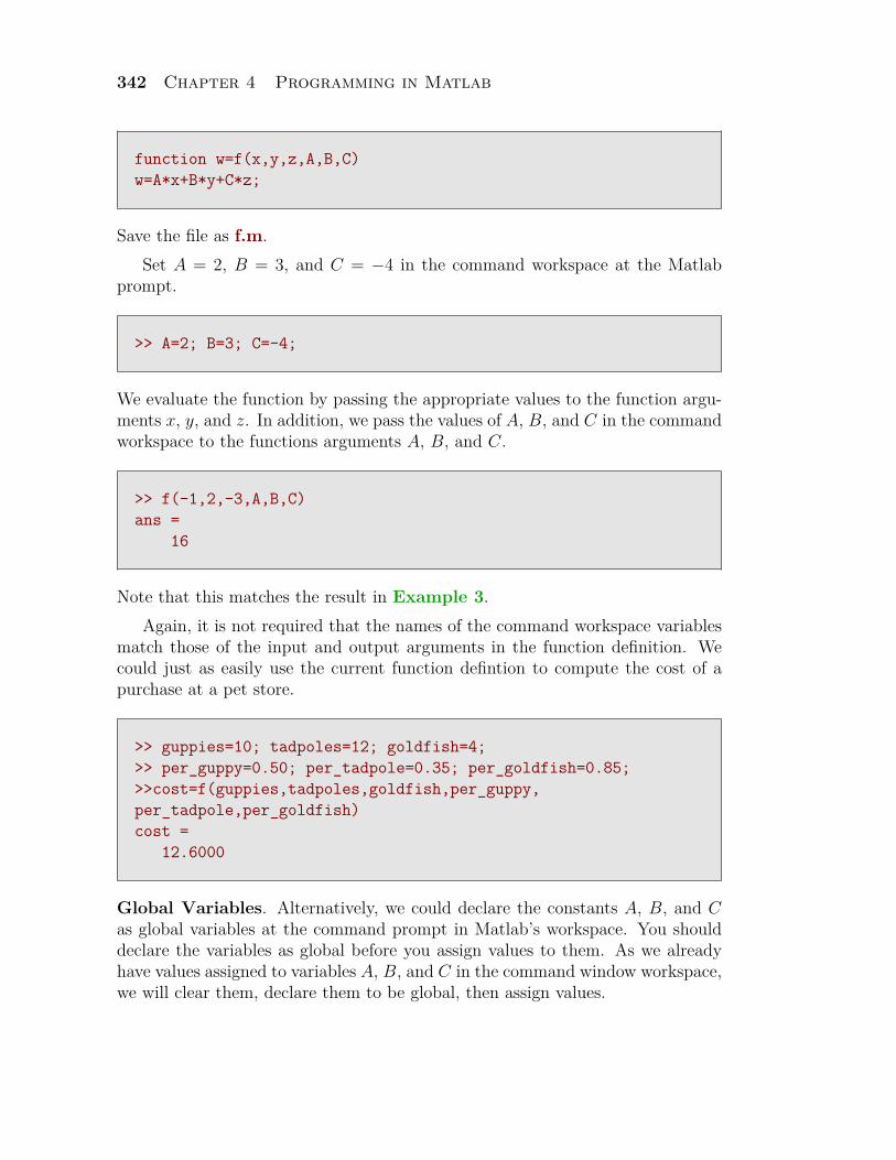
342 Chapter 4 Programming in Matlab
function w=f(x,y,z,A,B,C)w=A*x+B*y+C*z;
Save the file as f.m.Set A = 2, B = 3, and C = −4 in the command workspace at the Matlab
prompt.
>> A=2; B=3; C=-4;
We evaluate the function by passing the appropriate values to the function argu-ments x, y, and z. In addition, we pass the values of A, B, and C in the commandworkspace to the functions arguments A, B, and C.
>> f(-1,2,-3,A,B,C)ans =
16
Note that this matches the result in Example 3.Again, it is not required that the names of the command workspace variables
match those of the input and output arguments in the function definition. Wecould just as easily use the current function defintion to compute the cost of apurchase at a pet store.
>> guppies=10; tadpoles=12; goldfish=4;>> per_guppy=0.50; per_tadpole=0.35; per_goldfish=0.85;>>cost=f(guppies,tadpoles,goldfish,per_guppy,per_tadpole,per_goldfish)cost =
12.6000
Global Variables. Alternatively, we could declare the constants A, B, and Cas global variables at the command prompt in Matlab’s workspace. You shoulddeclare the variables as global before you assign values to them. As we alreadyhave values assigned to variables A, B, and C in the command window workspace,we will clear them, declare them to be global, then assign values.
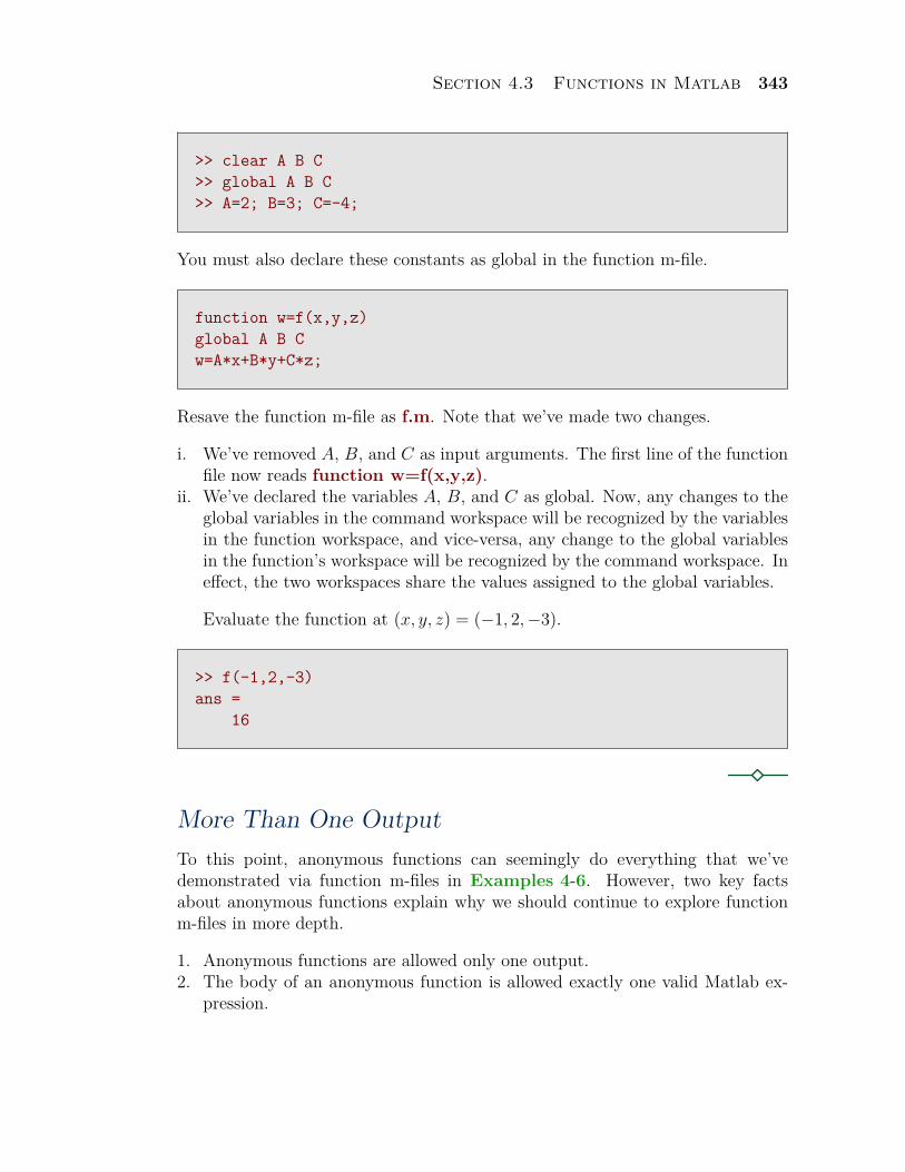
Section 4.3 Functions in Matlab 343
>> clear A B C>> global A B C>> A=2; B=3; C=-4;
You must also declare these constants as global in the function m-file.
function w=f(x,y,z)global A B Cw=A*x+B*y+C*z;
Resave the function m-file as f.m. Note that we’ve made two changes.
i. We’ve removed A, B, and C as input arguments. The first line of the functionfile now reads function w=f(x,y,z).
ii. We’ve declared the variables A, B, and C as global. Now, any changes to theglobal variables in the command workspace will be recognized by the variablesin the function workspace, and vice-versa, any change to the global variablesin the function’s workspace will be recognized by the command workspace. Ineffect, the two workspaces share the values assigned to the global variables.
Evaluate the function at (x, y, z) = (−1, 2,−3).
>> f(-1,2,-3)ans =
16
More Than One OutputTo this point, anonymous functions can seemingly do everything that we’vedemonstrated via function m-files in Examples 4-6. However, two key factsabout anonymous functions explain why we should continue to explore functionm-files in more depth.
1. Anonymous functions are allowed only one output.2. The body of an anonymous function is allowed exactly one valid Matlab ex-
pression.
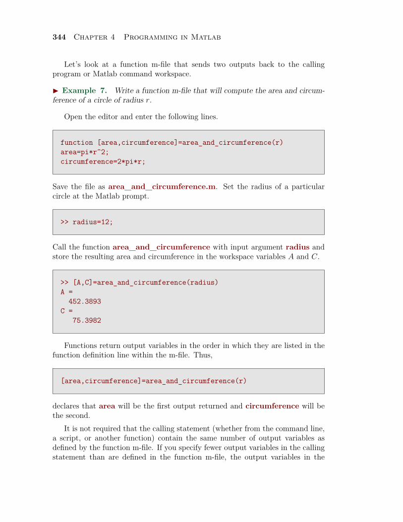
344 Chapter 4 Programming in Matlab
Let’s look at a function m-file that sends two outputs back to the callingprogram or Matlab command workspace.
I Example 7. Write a function m-file that will compute the area and circum-ference of a circle of radius r.
Open the editor and enter the following lines.
function [area,circumference]=area_and_circumference(r)area=pi*r^2;circumference=2*pi*r;
Save the file as area_and_circumference.m. Set the radius of a particularcircle at the Matlab prompt.
>> radius=12;
Call the function area_and_circumference with input argument radius andstore the resulting area and circumference in the workspace variables A and C.
>> [A,C]=area_and_circumference(radius)A =
452.3893C =
75.3982
Functions return output variables in the order in which they are listed in thefunction definition line within the m-file. Thus,
[area,circumference]=area_and_circumference(r)
declares that area will be the first output returned and circumference will bethe second.
It is not required that the calling statement (whether from the command line,a script, or another function) contain the same number of output variables asdefined by the function m-file. If you specify fewer output variables in the callingstatement than are defined in the function m-file, the output variables in the
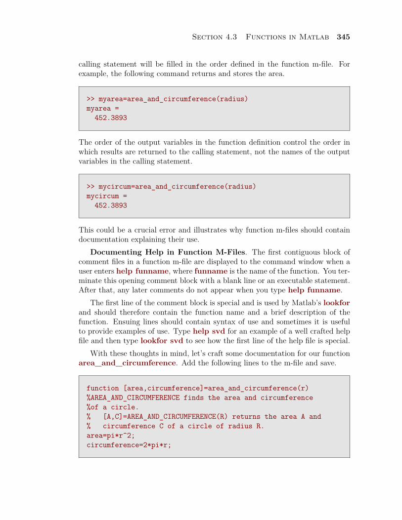
Section 4.3 Functions in Matlab 345
calling statement will be filled in the order defined in the function m-file. Forexample, the following command returns and stores the area.
>> myarea=area_and_circumference(radius)myarea =
452.3893
The order of the output variables in the function definition control the order inwhich results are returned to the calling statement, not the names of the outputvariables in the calling statement.
>> mycircum=area_and_circumference(radius)mycircum =
452.3893
This could be a crucial error and illustrates why function m-files should containdocumentation explaining their use.
Documenting Help in Function M-Files. The first contiguous block ofcomment files in a function m-file are displayed to the command window when auser enters help funname, where funname is the name of the function. You ter-minate this opening comment block with a blank line or an executable statement.After that, any later comments do not appear when you type help funname.
The first line of the comment block is special and is used by Matlab’s lookforand should therefore contain the function name and a brief description of thefunction. Ensuing lines should contain syntax of use and sometimes it is usefulto provide examples of use. Type help svd for an example of a well crafted helpfile and then type lookfor svd to see how the first line of the help file is special.
With these thoughts in mind, let’s craft some documentation for our functionarea_and_circumference. Add the following lines to the m-file and save.
function [area,circumference]=area_and_circumference(r)%AREA_AND_CIRCUMFERENCE finds the area and circumference%of a circle.% [A,C]=AREA_AND_CIRCUMFERENCE(R) returns the area A and% circumference C of a circle of radius R.area=pi*r^2;circumference=2*pi*r;
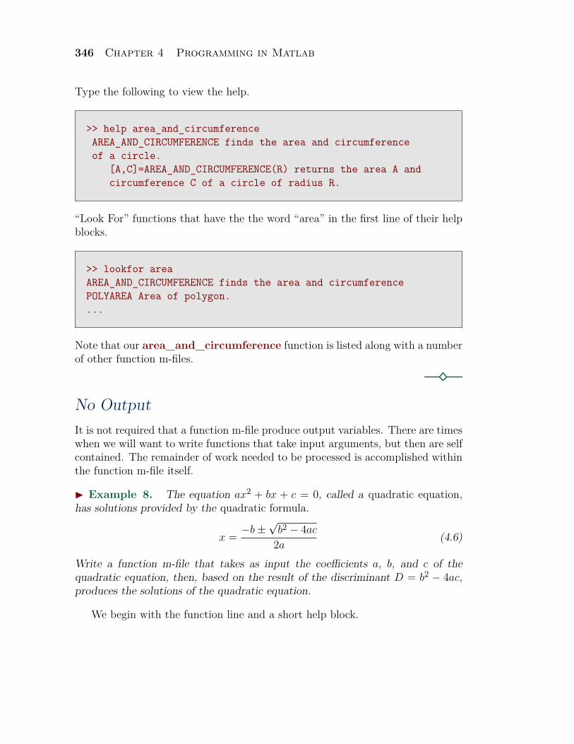
346 Chapter 4 Programming in Matlab
Type the following to view the help.
>> help area_and_circumferenceAREA_AND_CIRCUMFERENCE finds the area and circumferenceof a circle.
[A,C]=AREA_AND_CIRCUMFERENCE(R) returns the area A andcircumference C of a circle of radius R.
“Look For” functions that have the the word “area” in the first line of their helpblocks.
>> lookfor areaAREA_AND_CIRCUMFERENCE finds the area and circumferencePOLYAREA Area of polygon....
Note that our area_and_circumference function is listed along with a numberof other function m-files.
No OutputIt is not required that a function m-file produce output variables. There are timeswhen we will want to write functions that take input arguments, but then are selfcontained. The remainder of work needed to be processed is accomplished withinthe function m-file itself.
I Example 8. The equation ax2 + bx + c = 0, called a quadratic equation,has solutions provided by the quadratic formula.
x = −b±√
b2 − 4ac
2a(4.6)
Write a function m-file that takes as input the coefficients a, b, and c of thequadratic equation, then, based on the result of the discriminant D = b2 − 4ac,produces the solutions of the quadratic equation.
We begin with the function line and a short help block.
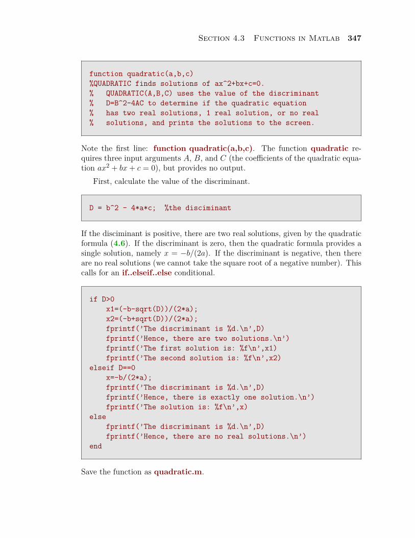
Section 4.3 Functions in Matlab 347
function quadratic(a,b,c)%QUADRATIC finds solutions of ax^2+bx+c=0.% QUADRATIC(A,B,C) uses the value of the discriminant% D=B^2-4AC to determine if the quadratic equation% has two real solutions, 1 real solution, or no real% solutions, and prints the solutions to the screen.
Note the first line: function quadratic(a,b,c). The function quadratic re-quires three input arguments A, B, and C (the coefficients of the quadratic equa-tion ax2 + bx + c = 0), but provides no output.
First, calculate the value of the discriminant.
D = b^2 - 4*a*c; %the disciminant
If the disciminant is positive, there are two real solutions, given by the quadraticformula (4.6). If the discriminant is zero, then the quadratic formula provides asingle solution, namely x = −b/(2a). If the discriminant is negative, then thereare no real solutions (we cannot take the square root of a negative number). Thiscalls for an if..elseif..else conditional.
if D>0x1=(-b-sqrt(D))/(2*a);x2=(-b+sqrt(D))/(2*a);fprintf(’The discriminant is %d.\n’,D)fprintf(’Hence, there are two solutions.\n’)fprintf(’The first solution is: %f\n’,x1)fprintf(’The second solution is: %f\n’,x2)
elseif D==0x=-b/(2*a);fprintf(’The discriminant is %d.\n’,D)fprintf(’Hence, there is exactly one solution.\n’)fprintf(’The solution is: %f\n’,x)
elsefprintf(’The discriminant is %d.\n’,D)fprintf(’Hence, there are no real solutions.\n’)
end
Save the function as quadratic.m.
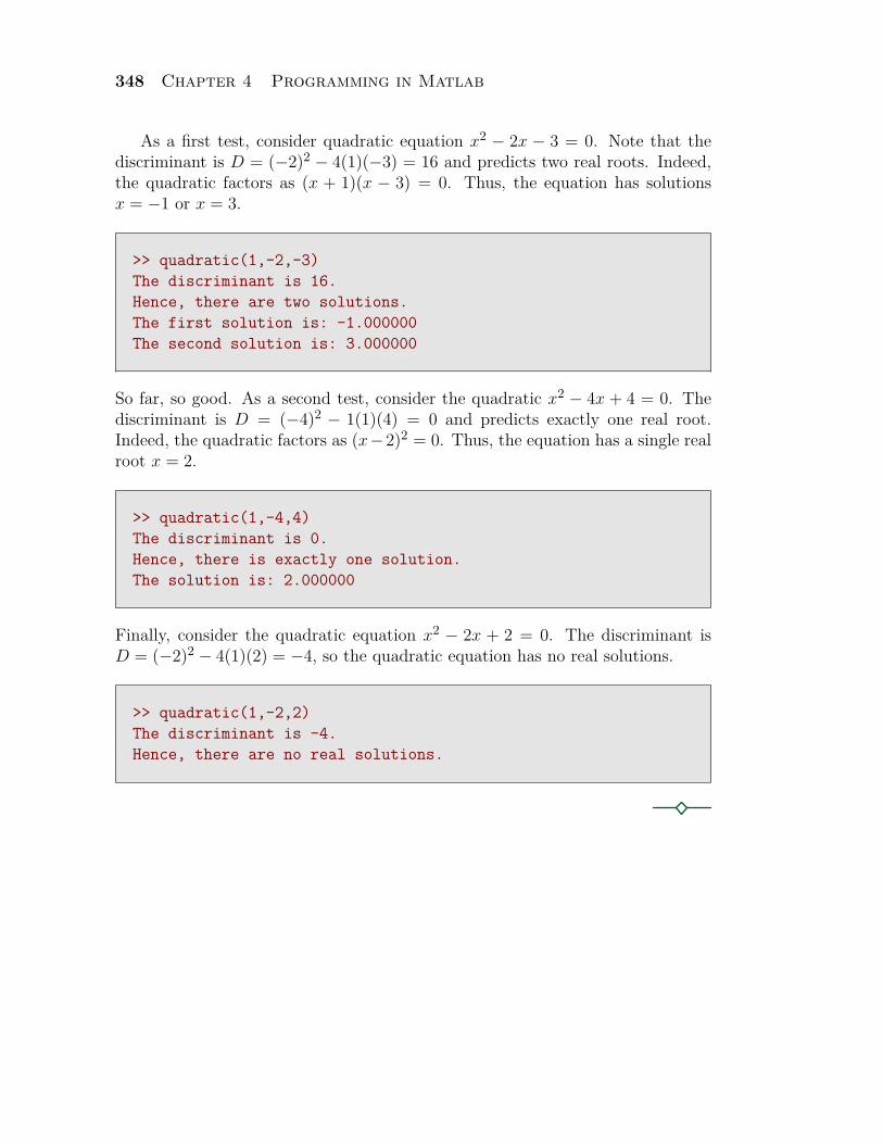
348 Chapter 4 Programming in Matlab
As a first test, consider quadratic equation x2 − 2x − 3 = 0. Note that thediscriminant is D = (−2)2 − 4(1)(−3) = 16 and predicts two real roots. Indeed,the quadratic factors as (x + 1)(x − 3) = 0. Thus, the equation has solutionsx = −1 or x = 3.
>> quadratic(1,-2,-3)The discriminant is 16.Hence, there are two solutions.The first solution is: -1.000000The second solution is: 3.000000
So far, so good. As a second test, consider the quadratic x2 − 4x + 4 = 0. Thediscriminant is D = (−4)2 − 1(1)(4) = 0 and predicts exactly one real root.Indeed, the quadratic factors as (x−2)2 = 0. Thus, the equation has a single realroot x = 2.
>> quadratic(1,-4,4)The discriminant is 0.Hence, there is exactly one solution.The solution is: 2.000000
Finally, consider the quadratic equation x2 − 2x + 2 = 0. The discriminant isD = (−2)2 − 4(1)(2) = −4, so the quadratic equation has no real solutions.
>> quadratic(1,-2,2)The discriminant is -4.Hence, there are no real solutions.
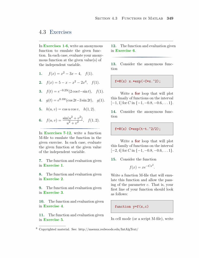
Section 4.3 Functions in Matlab 349
4.3 Exercises
In Exercises 1-6, write an anonymousfunction to emulate the given func-tion. In each case, evaluate your anony-mous function at the given value(s) ofthe independent variable.
1. f(x) = x2 − 3x− 4, f(1).
2. f(x) = 5− x− x2 − 2x4, f(1).
3. f(t) = e−0.25t(2 cos t−sin t), f(1).
4. g(t) = e0.10t(cos 2t−3 sin 2t), g(1).
5. h(u, v) = cos u cos v, h(1, 2).
6. f(u, v) = sin(u2 + v2)u2 + v2 , f(1, 2).
In Exercises 7-12, write a functionM-file to emulate the function in thegiven exercise. In each case, evaluatethe given function at the given valueof the independent variable.
7. The function and evaluation givenin Exercise 1.
8. The function and evaluation givenin Exercise 2.
9. The function and evaluation givenin Exercise 3.
10. The function and evaluation givenin Exercise 4.
11. The function and evaluation givenin Exercise 5.
Copyrighted material. See: http://msenux.redwoods.edu/IntAlgText/8
12. The function and evaluation givenin Exercise 6.
13. Consider the anonymous func-tion
f=@(x) x.*exp(-C*x.^2);
Write a for loop that will plotthis fmaily of functions on the interval[−1, 1] for C in {−1,−0.8,−0.6, . . . 1}.
14. Consider the anonymous func-tion
f=@(x) C*exp(t-t.^2/2);
Write a for loop that will plotthis family of functions on the interval[−2, 4] for C in {−1,−0.8,−0.6, . . . 1}.
15. Consider the function
f(x) = xe−Cx2.
Write a function M-file that will emu-late this function and allow the pass-ing of the parameter c. That is, yourfirst line of your function should lookas follows:
function y=f(x,c)
In cell mode (or a script M-file), write
350 Chapter 4 Programming in Matlab
a for loop that will plot this family offunctions on the interval [−1, 1] for Cin {−1,−0.8,−0.6, . . . 1}.
16. Consider the function
f(x) = cex−x2/2.
Write a function M-file that will emu-late this function and allow the pass-ing of the parameter c. That is, yourfirst line of your function should lookas follows:
function y=f(x,c)
In cell mode (or a script M-file), writea for loop that will plot this family offunctions on the interval [−2, 4] for Cin {−1,−0.8,−0.6, . . . 1}.
17. The sequence
1, 1, 2, 3, . . . , an−2, an−1, an, . . .
where an = an−2 + an−1, is called aFibonacci sequence. Write a functionthat will return the nth term of theFibonacci sequence. The first line ofyour function should read as follows.
function term=fib(n)
Call this function from cell mode (or ascript M-file) and format the output.
18. Adjust the function M-file cre-ated in Exercise 17 so that it returnsa vector containing the first n termsof the Fibonacci sequence. Call thisfunction from cell mode (or a scriptM-file) and format the output.
19. Euclid proved that there were aninfinite number of primes. He also be-lieved that there was an infinite num-ber ot twin primes, primes that differby 2 (like 5 and 7 or 11 and 13), butno one has been able to prove this con-jecture for the past 2300 years. Writea function that will produce all twinprimes between two inputs, integers aand b.
20. In mathematics, a sexy prime isa pair of primes (p, p+6) that differ by6. Write a function that will produceall sexy primes between two inputs,integers a and b.
21. The factorial of nonnegative in-teger n is denoted by the mathematicnotation n! and is defined as follows.
n! ={
1, if n = 0n(n− 1)(n− 2) · · · 1, if n 6= 0
Write a function M-file myfactorialthat returns the factorial when a non-negative integer is received as input.Use cell mode (or a script M-file) totest your function at n = 0 and n = 5.Hint: Consider using Matlab’s prodfunction.
22. The binomial coefficient is de-fined by (
n
k
)= n!
k!(n− k)!.
Write a function M-file called binomthat takes two inputs, n and k, thenreturns the binomial coefficient. Usethe myfactorial function written inExercise 21. Use cell mode to testyour function for n = 5 and k = 2.
Section 4.3 Functions in Matlab 351
23. The first few rows of Pascal’s Tri-angle look like the following.
11 11 2 11 3 3 11 4 6 4 1
The nth row holds the binomialcoefficients(
n
k
), k = 0, 1, . . . , n.
Write a function to produce Pascal’sTriangle for an arbitrary number r ofrows. Your first line should read asfollows.
function pascalTriangle(r)
This function should use nested forloops to produce the rows of Pascal’sTriangle. The function should also usethe fprintf command to print eachrow to the screen. Use cell mode totest your function by entering the fol-lowing line in your cell enabled editor.
pascalTriangle(8)
Your function should employ the binomfunction written in Exercise 20. Hint:The format to use for the fprintf com-mand is the tricky part of this exer-cise. Before entering the inner loop tocompute the coefficients for a partic-ular row, set format=’’ (the emptystring), then build the string in the in-
ner loop with format=[format,’%6d’].Once the inner loop completes, you’llneed to add a line return character be-fore executing fprintf(format,row).
24. Rewrite the quadratic functionm-file of Example 8 by replacing theif..elseif..else conditional with Mat-lab’s switch..case..otherwise condi-tional.
25. Rewrite the quadratic functionm-file of Example 8 to produce twocomplex solutions of the quadratic equa-tion ax2 +bx+c = 0 in the case wherethe discriminant D = b2 − 4ac < 0.
26. Write a function called mysortthat will take a column vector of num-bers as input, sort them in ascendingorder, then return the sorted list as acolumn vector. Test the speed of yourroutine with the following commands.
in=rand(10000,1);>> tic, mysort(in); toc
Compare the speed of your sort-ing routine with Matlab’s.
>> tic, sort(in); toc
Note: This is a classic problemin computer science, a ritual of pas-sage, like crossing the equator for thefirst time. There are very sophisti-cated algorithms for attacking this prob-lem, but try to see what you can dowith it on your own instead of search-ing for a sort routine on the internet.
352 Chapter 4 Programming in Matlab
27. Write a function called mymaxthat will take a column vector of num-bers as input and find the largest en-try. The routine should spit out twonumbers, the largest entry m and itsposition k in the vector. Test the speedof your routine with the following com-mands.
in=rand(1000000,1);>> tic, [m,k]=mymax(in); toc
Compare the speed of your max-imum routine with Matlab’s.
>> tic, [m,k]=max(in); toc
28. Write a function called myminthat will take a column vector of num-bers as input and find the smallest en-try. The routine should spit out twonumbers, the smallest entry m andits position k in the vector. Test thespeed of your routine with the follow-ing commands.
in=rand(10000,1);>> tic, [m,k]=mymin(in); toc
Compare the speed of your max-imum routine with Matlab’s.
>> tic, [m,k]=min(in); toc
29. According to Wikipedia, the so-lutions to the cubic equation
ax3 + bx2 + cx + d = 0
are found as follows. First, compute
q = 3ac− b2
9a2
and
r = 9abc− 27a2d− 2b3
54a3 .
Next, compute
s = 3√
r +√
q3 + r2
and
t = 3√
r −√
q3 + r2.
The solutions are, first,
x1 = s + t− b
3a,
then
x2 = −s + t
2− b
3a+√
32
(s− t)i,
and
x3 = −s + t
2− b
3a−√
32
(s− t)i,
where i =√−1. Write a function to
compute the roots of the cubic equa-tion. The first line should read as fol-lows.
function [x1,x2,x3]=cardano(a,b,c,d)
Set up a test to verify that your imple-mentation of the solution of the cubicequation is working correctly.
Section 4.3 Functions in Matlab 353
4.3 Answers
1.
>> f=@(x) x^2-3*x-4;>> f(1)ans =
-6
3.
>> f=@(t) exp(-0.25*t)*(2*cos(t)-sin(t));>> f(1)ans =
0.1862
5.
>> h=@(u,v) cos(u)*cos(v);>> h(1,2)ans =
-0.2248
7. The function M-file:
function y=f(x)y=x^2-3*x-4;
Calling the function from the command line.
354 Chapter 4 Programming in Matlab
>> f(1)ans =
-6
9. The function M-file:
function y=f(t)y=exp(-0.25*t)*(2*cos(t)-sin(t));
Calling the function from the command line.
>> f(1)ans =
0.1862
11. The function M-file:
function z=h(u,v)z=cos(u)*cos(v);
Calling the function from the command line.
>> h(1,2)ans =
-0.2248
13. Set the domain.
x=linspace(-1,1);
Write the for loop.
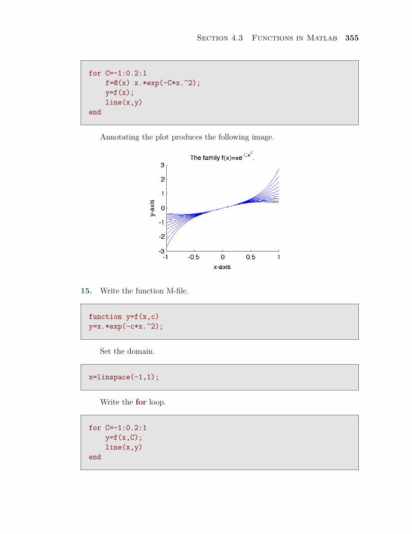
Section 4.3 Functions in Matlab 355
for C=-1:0.2:1f=@(x) x.*exp(-C*x.^2);y=f(x);line(x,y)
end
Annotating the plot produces the following image.
15. Write the function M-file.
function y=f(x,c)y=x.*exp(-c*x.^2);
Set the domain.
x=linspace(-1,1);
Write the for loop.
for C=-1:0.2:1y=f(x,C);line(x,y)
end
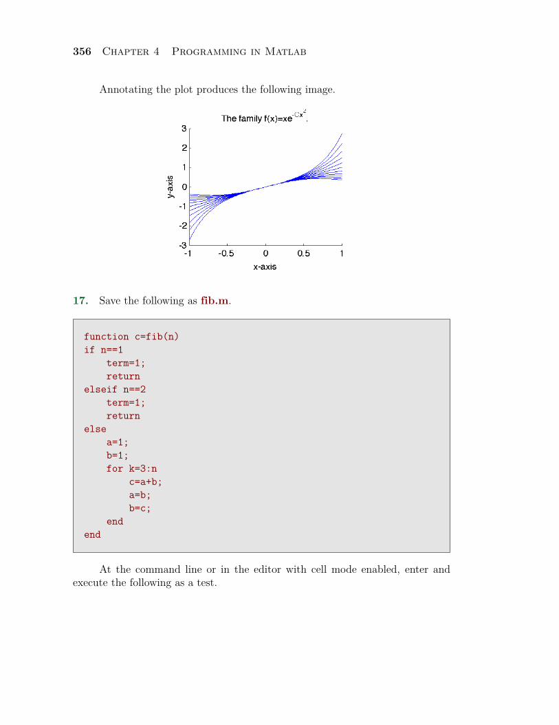
356 Chapter 4 Programming in Matlab
Annotating the plot produces the following image.
17. Save the following as fib.m.
function c=fib(n)if n==1
term=1;return
elseif n==2term=1;return
elsea=1;b=1;for k=3:n
c=a+b;a=b;b=c;
endend
At the command line or in the editor with cell mode enabled, enter andexecute the following as a test.
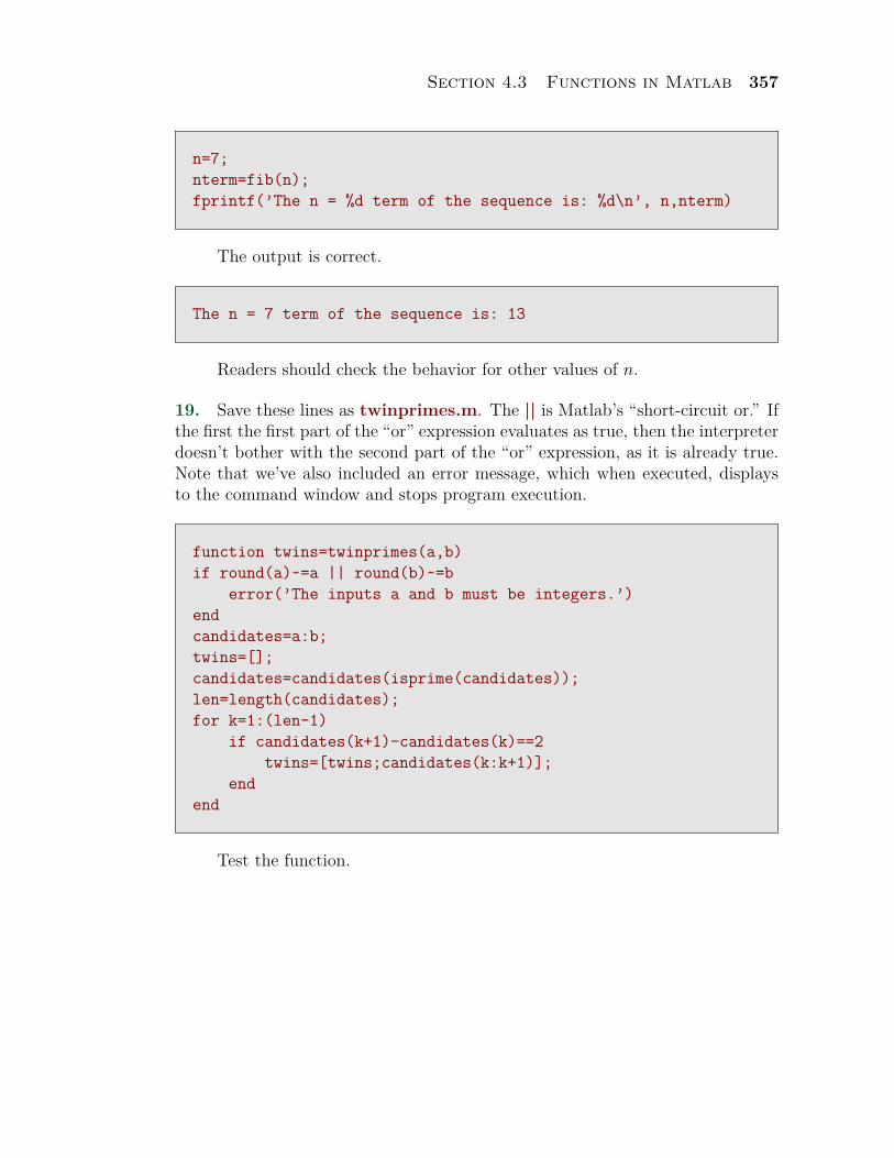
Section 4.3 Functions in Matlab 357
n=7;nterm=fib(n);fprintf(’The n = %d term of the sequence is: %d\n’, n,nterm)
The output is correct.
The n = 7 term of the sequence is: 13
Readers should check the behavior for other values of n.
19. Save these lines as twinprimes.m. The || is Matlab’s “short-circuit or.” Ifthe first the first part of the “or” expression evaluates as true, then the interpreterdoesn’t bother with the second part of the “or” expression, as it is already true.Note that we’ve also included an error message, which when executed, displaysto the command window and stops program execution.
function twins=twinprimes(a,b)if round(a)~=a || round(b)~=b
error(’The inputs a and b must be integers.’)endcandidates=a:b;twins=[];candidates=candidates(isprime(candidates));len=length(candidates);for k=1:(len-1)
if candidates(k+1)-candidates(k)==2twins=[twins;candidates(k:k+1)];
endend
Test the function.
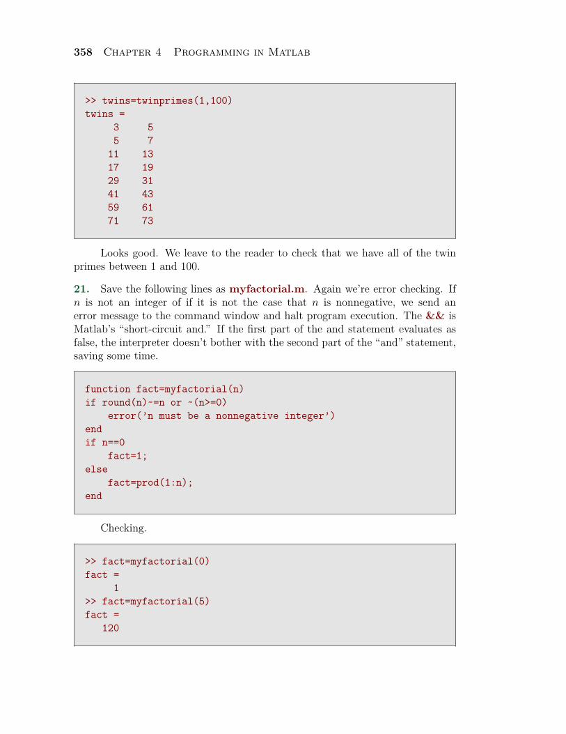
358 Chapter 4 Programming in Matlab
>> twins=twinprimes(1,100)twins =
3 55 7
11 1317 1929 3141 4359 6171 73
Looks good. We leave to the reader to check that we have all of the twinprimes between 1 and 100.
21. Save the following lines as myfactorial.m. Again we’re error checking. Ifn is not an integer of if it is not the case that n is nonnegative, we send anerror message to the command window and halt program execution. The && isMatlab’s “short-circuit and.” If the first part of the and statement evaluates asfalse, the interpreter doesn’t bother with the second part of the “and” statement,saving some time.
function fact=myfactorial(n)if round(n)~=n or ~(n>=0)
error(’n must be a nonnegative integer’)endif n==0
fact=1;else
fact=prod(1:n);end
Checking.
>> fact=myfactorial(0)fact =
1>> fact=myfactorial(5)fact =
120
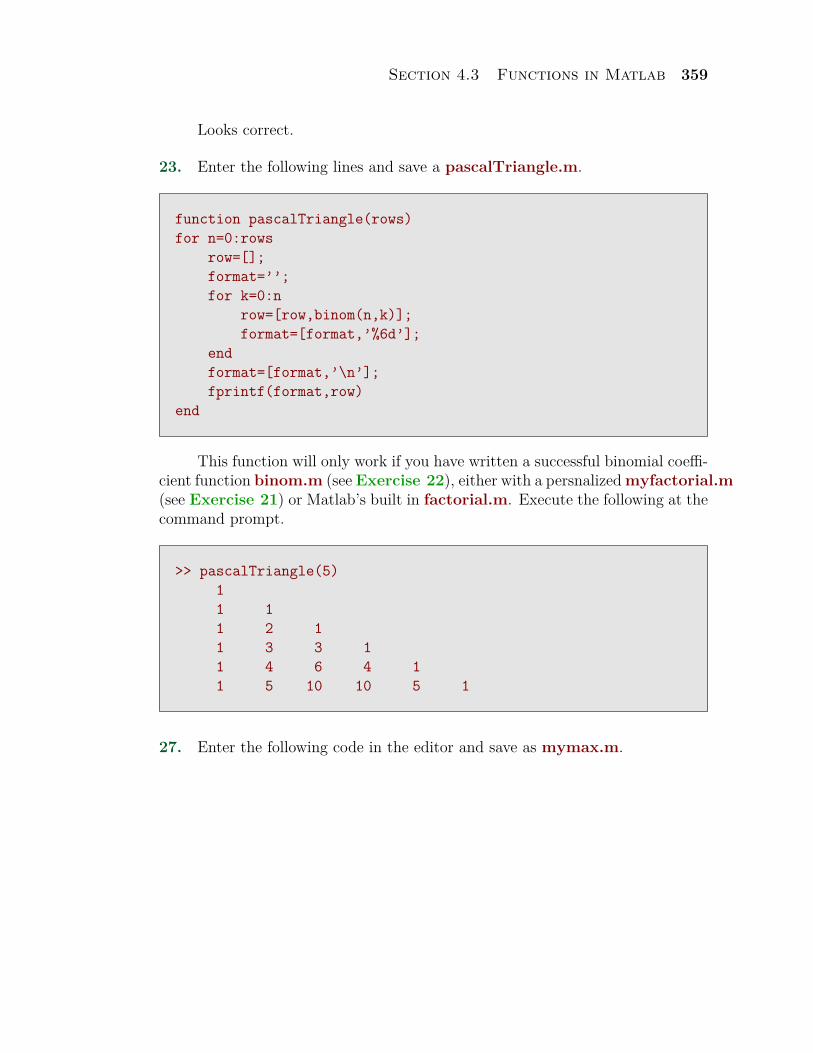
Section 4.3 Functions in Matlab 359
Looks correct.
23. Enter the following lines and save a pascalTriangle.m.
function pascalTriangle(rows)for n=0:rows
row=[];format=’’;for k=0:n
row=[row,binom(n,k)];format=[format,’%6d’];
endformat=[format,’\n’];fprintf(format,row)
end
This function will only work if you have written a successful binomial coeffi-cient function binom.m (see Exercise 22), either with a persnalized myfactorial.m(see Exercise 21) or Matlab’s built in factorial.m. Execute the following at thecommand prompt.
>> pascalTriangle(5)11 11 2 11 3 3 11 4 6 4 11 5 10 10 5 1
27. Enter the following code in the editor and save as mymax.m.
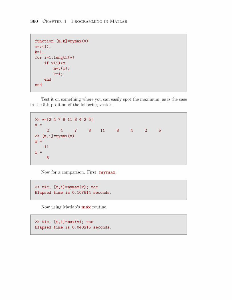
360 Chapter 4 Programming in Matlab
function [m,k]=mymax(v)m=v(1);k=1;for i=1:length(v)
if v(i)>mm=v(i);k=i;
endend
Test it on something where you can easily spot the maximum, as is the casein the 5th position of the following vector.
>> v=[2 4 7 8 11 8 4 2 5]v =
2 4 7 8 11 8 4 2 5>> [m,i]=mymax(v)m =
11i =
5
Now for a comparison. First, mymax.
>> tic, [m,i]=mymax(v); tocElapsed time is 0.107614 seconds.
Now using Matlab’s max routine.
>> tic, [m,i]=max(v); tocElapsed time is 0.040215 seconds.
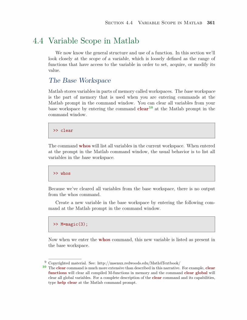
Section 4.4 Variable Scope in Matlab 361
4.4 Variable Scope in MatlabWe now know the general structure and use of a function. In this section we’ll
look closely at the scope of a variable, which is loosely defined as the range offunctions that have access to the variable in order to set, acquire, or modify itsvalue.
The Base WorkspaceMatlab stores variables in parts of memory called workspaces. The base workspaceis the part of memory that is used when you are entering commands at theMatlab prompt in the command window. You can clear all variables from yourbase workspace by entering the command clear10 at the Matlab prompt in thecommand window.
>> clear
The command whos will list all variables in the current workspace. When enteredat the prompt in the Matlab command window, the usual behavior is to list allvariables in the base workspace.
>> whos
Because we’ve cleared all variables from the base workspace, there is no outputfrom the whos command.
Create a new variable in the base workspace by entering the following com-mand at the Matlab prompt in the command window.
>> M=magic(3);
Now when we enter the whos command, this new variable is listed as present inthe base workspace.
Copyrighted material. See: http://msenux.redwoods.edu/Math4Textbook/9
The clear command is much more extensive than described in this narrative. For example, clear10
functions will clear all compiled M-functions in memory and the command clear global willclear all global variables. For a complete description of the clear command and its capabilities,type help clear at the Matlab command prompt.
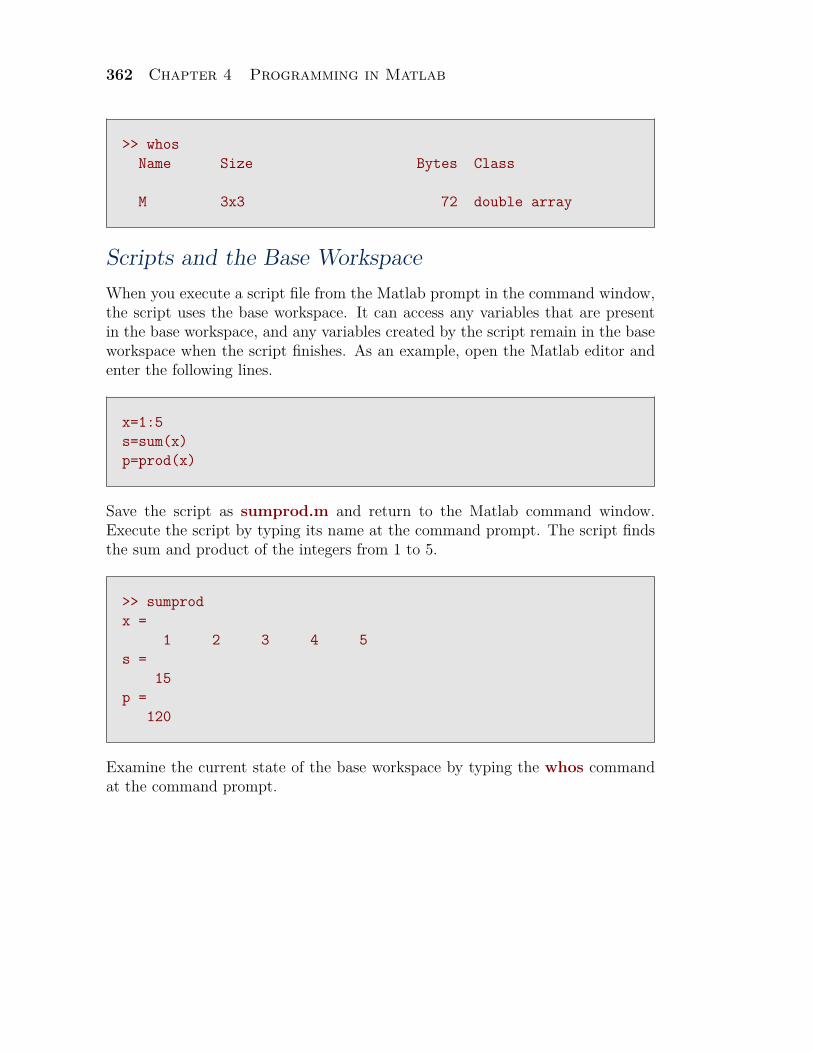
362 Chapter 4 Programming in Matlab
>> whosName Size Bytes Class
M 3x3 72 double array
Scripts and the Base WorkspaceWhen you execute a script file from the Matlab prompt in the command window,the script uses the base workspace. It can access any variables that are presentin the base workspace, and any variables created by the script remain in the baseworkspace when the script finishes. As an example, open the Matlab editor andenter the following lines.
x=1:5s=sum(x)p=prod(x)
Save the script as sumprod.m and return to the Matlab command window.Execute the script by typing its name at the command prompt. The script findsthe sum and product of the integers from 1 to 5.
>> sumprodx =
1 2 3 4 5s =
15p =
120
Examine the current state of the base workspace by typing the whos commandat the command prompt.
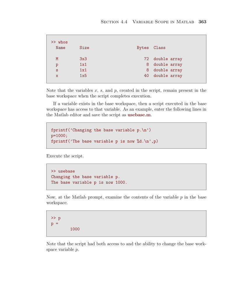
Section 4.4 Variable Scope in Matlab 363
>> whosName Size Bytes Class
M 3x3 72 double arrayp 1x1 8 double arrays 1x1 8 double arrayx 1x5 40 double array
Note that the variables x, s, and p, created in the script, remain present in thebase workspace when the script completes execution.
If a variable exists in the base workspace, then a script executed in the baseworkspace has access to that variable. As an example, enter the following lines inthe Matlab editor and save the script as usebase.m.
fprintf(’Changing the base variable p.\n’)p=1000;fprintf(’The base variable p is now %d.\n’,p)
Execute the script.
>> usebaseChanging the base variable p.The base variable p is now 1000.
Now, at the Matlab prompt, examine the contents of the variable p in the baseworkspace.
>> pp =
1000
Note that the script had both access to and the ability to change the base work-space variable p.
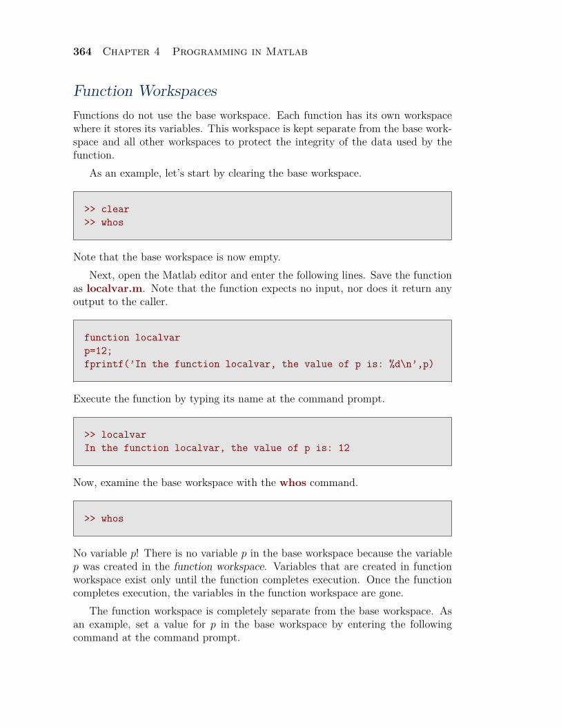
364 Chapter 4 Programming in Matlab
Function WorkspacesFunctions do not use the base workspace. Each function has its own workspacewhere it stores its variables. This workspace is kept separate from the base work-space and all other workspaces to protect the integrity of the data used by thefunction.
As an example, let’s start by clearing the base workspace.
>> clear>> whos
Note that the base workspace is now empty.Next, open the Matlab editor and enter the following lines. Save the function
as localvar.m. Note that the function expects no input, nor does it return anyoutput to the caller.
function localvarp=12;fprintf(’In the function localvar, the value of p is: %d\n’,p)
Execute the function by typing its name at the command prompt.
>> localvarIn the function localvar, the value of p is: 12
Now, examine the base workspace with the whos command.
>> whos
No variable p! There is no variable p in the base workspace because the variablep was created in the function workspace. Variables that are created in functionworkspace exist only until the function completes execution. Once the functioncompletes execution, the variables in the function workspace are gone.
The function workspace is completely separate from the base workspace. Asan example, set a value for p in the base workspace by entering the followingcommand at the command prompt.
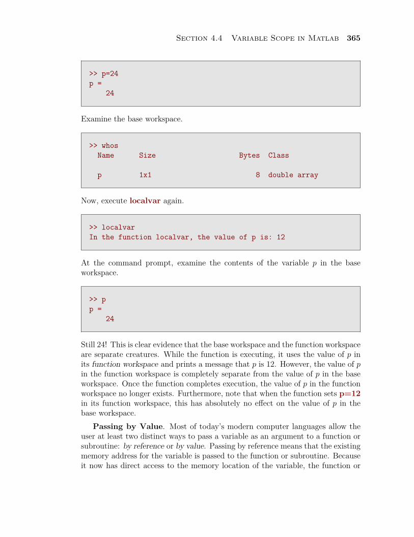
Section 4.4 Variable Scope in Matlab 365
>> p=24p =
24
Examine the base workspace.
>> whosName Size Bytes Class
p 1x1 8 double array
Now, execute localvar again.
>> localvarIn the function localvar, the value of p is: 12
At the command prompt, examine the contents of the variable p in the baseworkspace.
>> pp =
24
Still 24! This is clear evidence that the base workspace and the function workspaceare separate creatures. While the function is executing, it uses the value of p inits function workspace and prints a message that p is 12. However, the value of pin the function workspace is completely separate from the value of p in the baseworkspace. Once the function completes execution, the value of p in the functionworkspace no longer exists. Furthermore, note that when the function sets p=12in its function workspace, this has absolutely no effect on the value of p in thebase workspace.
Passing by Value. Most of today’s modern computer languages allow theuser at least two distinct ways to pass a variable as an argument to a function orsubroutine: by reference or by value. Passing by reference means that the existingmemory address for the variable is passed to the function or subroutine. Becauseit now has direct access to the memory location of the variable, the function or
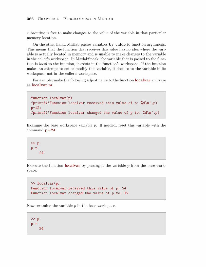
366 Chapter 4 Programming in Matlab
subroutine is free to make changes to the value of the variable in that particularmemory location.
On the other hand, Matlab passes variables by value to function arguments.This means that the function that receives this value has no idea where the vari-able is actually located in memory and is unable to make changes to the variablein the caller’s workspace. In MatlabSpeak, the variable that is passed to the func-tion is local to the function, it exists in the function’s workspace. If the functionmakes an attempt to set or modify this variable, it does so to the variable in itsworkspace, not in the caller’s workspace.
For eample, make the following adjustments to the function localvar and saveas localvar.m.
function localvar(p)fprintf(’Function localvar received this value of p: %d\n’,p)p=12;fprintf(’Function localvar changed the value of p to: %d\n’,p)
Examine the base workspace variable p. If needed, reset this variable with thecommand p=24.
>> pp =
24
Execute the function localvar by passing it the variable p from the base work-space.
>> localvar(p)Function localvar received this value of p: 24Function localvar changed the value of p to: 12
Now, examine the variable p in the base workspace.
>> pp =
24
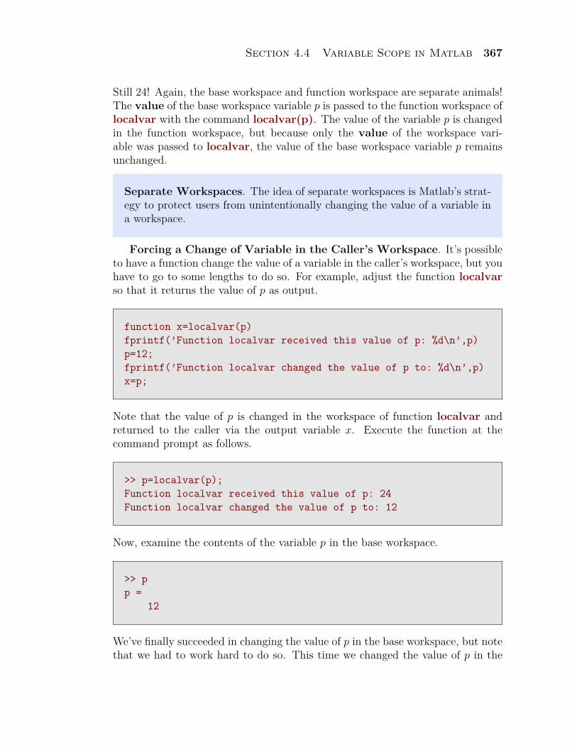
Section 4.4 Variable Scope in Matlab 367
Still 24! Again, the base workspace and function workspace are separate animals!The value of the base workspace variable p is passed to the function workspace oflocalvar with the command localvar(p). The value of the variable p is changedin the function workspace, but because only the value of the workspace vari-able was passed to localvar, the value of the base workspace variable p remainsunchanged.
Separate Workspaces. The idea of separate workspaces is Matlab’s strat-egy to protect users from unintentionally changing the value of a variable ina workspace.
Forcing a Change of Variable in the Caller’s Workspace. It’s possibleto have a function change the value of a variable in the caller’s workspace, but youhave to go to some lengths to do so. For example, adjust the function localvarso that it returns the value of p as output.
function x=localvar(p)fprintf(’Function localvar received this value of p: %d\n’,p)p=12;fprintf(’Function localvar changed the value of p to: %d\n’,p)x=p;
Note that the value of p is changed in the workspace of function localvar andreturned to the caller via the output variable x. Execute the function at thecommand prompt as follows.
>> p=localvar(p);Function localvar received this value of p: 24Function localvar changed the value of p to: 12
Now, examine the contents of the variable p in the base workspace.
>> pp =
12
We’ve finally succeeded in changing the value of p in the base workspace, but notethat we had to work hard to do so. This time we changed the value of p in the
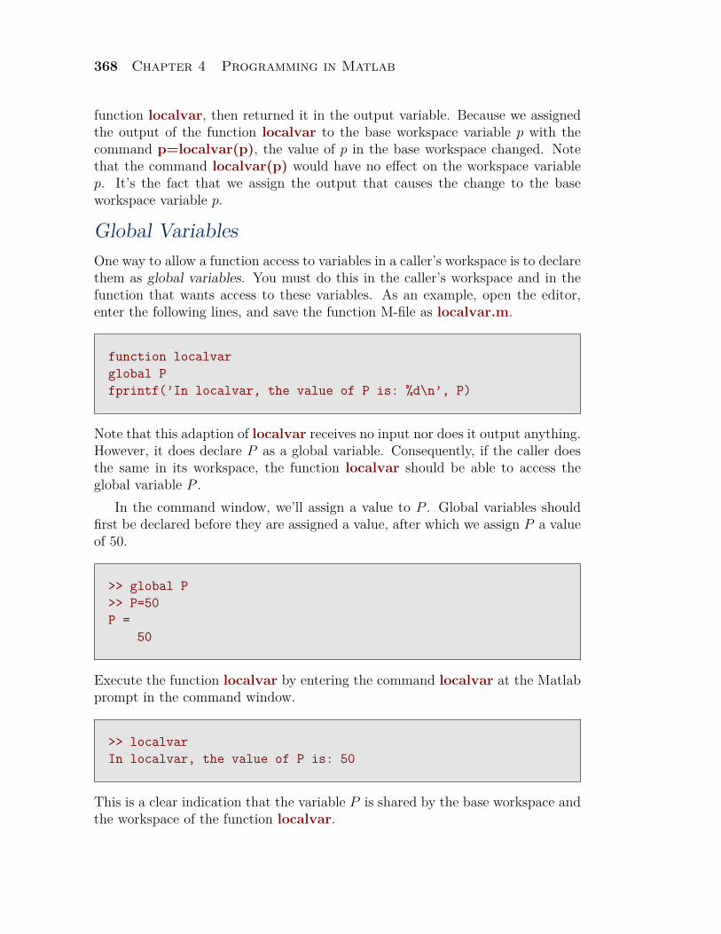
368 Chapter 4 Programming in Matlab
function localvar, then returned it in the output variable. Because we assignedthe output of the function localvar to the base workspace variable p with thecommand p=localvar(p), the value of p in the base workspace changed. Notethat the command localvar(p) would have no effect on the workspace variablep. It’s the fact that we assign the output that causes the change to the baseworkspace variable p.
Global VariablesOne way to allow a function access to variables in a caller’s workspace is to declarethem as global variables. You must do this in the caller’s workspace and in thefunction that wants access to these variables. As an example, open the editor,enter the following lines, and save the function M-file as localvar.m.
function localvarglobal Pfprintf(’In localvar, the value of P is: %d\n’, P)
Note that this adaption of localvar receives no input nor does it output anything.However, it does declare P as a global variable. Consequently, if the caller doesthe same in its workspace, the function localvar should be able to access theglobal variable P .
In the command window, we’ll assign a value to P . Global variables shouldfirst be declared before they are assigned a value, after which we assign P a valueof 50.
>> global P>> P=50P =
50
Execute the function localvar by entering the command localvar at the Matlabprompt in the command window.
>> localvarIn localvar, the value of P is: 50
This is a clear indication that the variable P is shared by the base workspace andthe workspace of the function localvar.
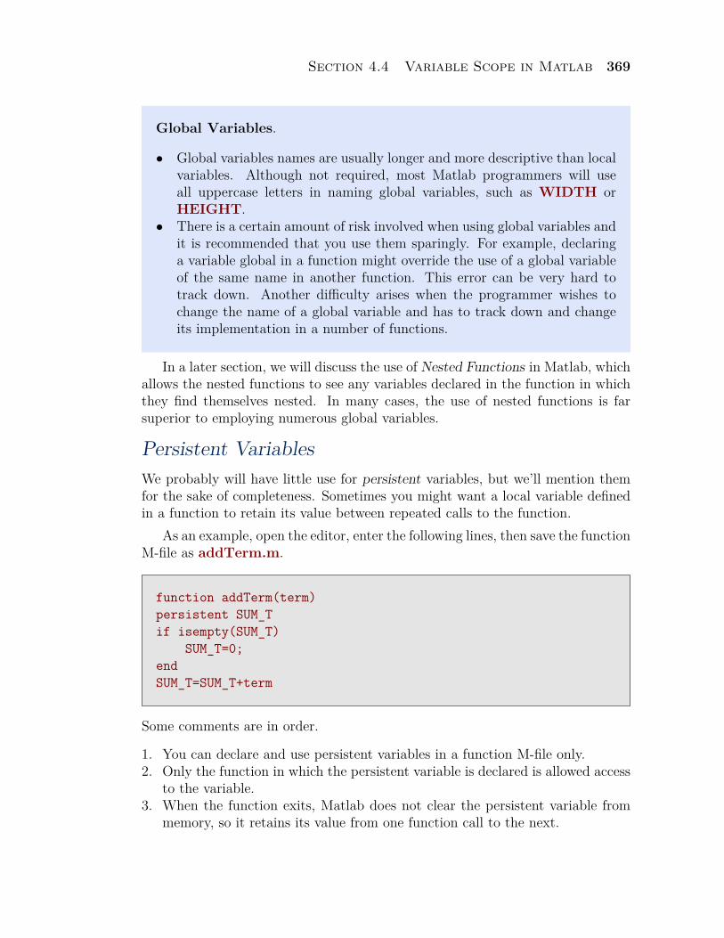
Section 4.4 Variable Scope in Matlab 369
Global Variables.
• Global variables names are usually longer and more descriptive than localvariables. Although not required, most Matlab programmers will useall uppercase letters in naming global variables, such as WIDTH orHEIGHT.
• There is a certain amount of risk involved when using global variables andit is recommended that you use them sparingly. For example, declaringa variable global in a function might override the use of a global variableof the same name in another function. This error can be very hard totrack down. Another difficulty arises when the programmer wishes tochange the name of a global variable and has to track down and changeits implementation in a number of functions.
In a later section, we will discuss the use of Nested Functions in Matlab, whichallows the nested functions to see any variables declared in the function in whichthey find themselves nested. In many cases, the use of nested functions is farsuperior to employing numerous global variables.
Persistent VariablesWe probably will have little use for persistent variables, but we’ll mention themfor the sake of completeness. Sometimes you might want a local variable definedin a function to retain its value between repeated calls to the function.
As an example, open the editor, enter the following lines, then save the functionM-file as addTerm.m.
function addTerm(term)persistent SUM_Tif isempty(SUM_T)
SUM_T=0;endSUM_T=SUM_T+term
Some comments are in order.
1. You can declare and use persistent variables in a function M-file only.2. Only the function in which the persistent variable is declared is allowed access
to the variable.3. When the function exits, Matlab does not clear the persistent variable from
memory, so it retains its value from one function call to the next.
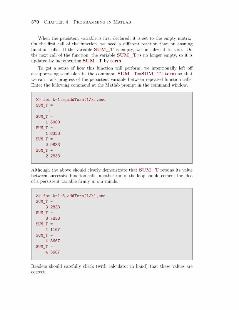
370 Chapter 4 Programming in Matlab
When the persistent variable is first declared, it is set to the empty matrix.On the first call of the function, we need a different reaction than on ensuingfunction calls. If the variable SUM_T is empty, we initialize it to zero. Onthe next call of the function, the variable SUM_T is no longer empty, so it isupdated by incrementing SUM_T by term.
To get a sense of how this function will perform, we intentionally left offa suppressing semicolon in the command SUM_T=SUM_T+term so thatwe can track progress of the persistent variable between repeated function calls.Enter the following command at the Matlab prompt in the command window.
>> for k=1:5,addTerm(1/k),endSUM_T =
1SUM_T =
1.5000SUM_T =
1.8333SUM_T =
2.0833SUM_T =
2.2833
Although the above should clearly demonstrate that SUM_T retains its valuebetween successive function calls, another run of the loop should cement the ideaof a persistent variable firmly in our minds.
>> for k=1:5,addTerm(1/k),endSUM_T =
3.2833SUM_T =
3.7833SUM_T =
4.1167SUM_T =
4.3667SUM_T =
4.5667
Readers should carefully check (with calculator in hand) that these values arecorrect.

Section 4.4 Variable Scope in Matlab 371
To clear a persistent variable from memory, you can use either clear the func-tion from memory clear addTerm or you can use the command clear all.
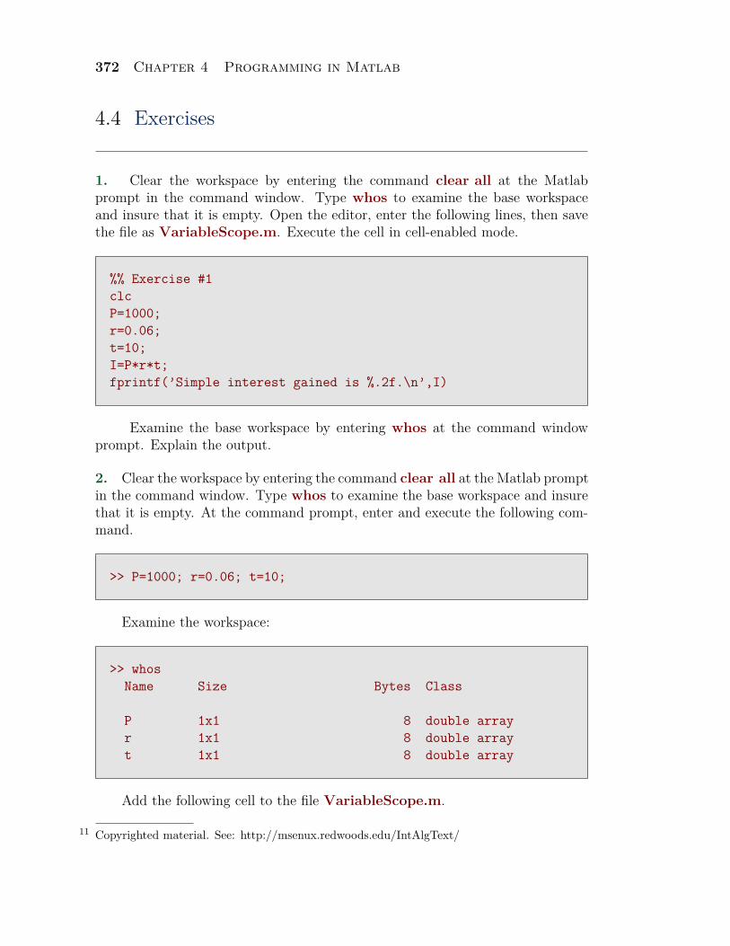
372 Chapter 4 Programming in Matlab
4.4 Exercises
1. Clear the workspace by entering the command clear all at the Matlabprompt in the command window. Type whos to examine the base workspaceand insure that it is empty. Open the editor, enter the following lines, then savethe file as VariableScope.m. Execute the cell in cell-enabled mode.
%% Exercise #1clcP=1000;r=0.06;t=10;I=P*r*t;fprintf(’Simple interest gained is %.2f.\n’,I)
Examine the base workspace by entering whos at the command windowprompt. Explain the output.
2. Clear the workspace by entering the command clear all at the Matlab promptin the command window. Type whos to examine the base workspace and insurethat it is empty. At the command prompt, enter and execute the following com-mand.
>> P=1000; r=0.06; t=10;
Examine the workspace:
>> whosName Size Bytes Class
P 1x1 8 double arrayr 1x1 8 double arrayt 1x1 8 double array
Add the following cell to the file VariableScope.m.
Copyrighted material. See: http://msenux.redwoods.edu/IntAlgText/11
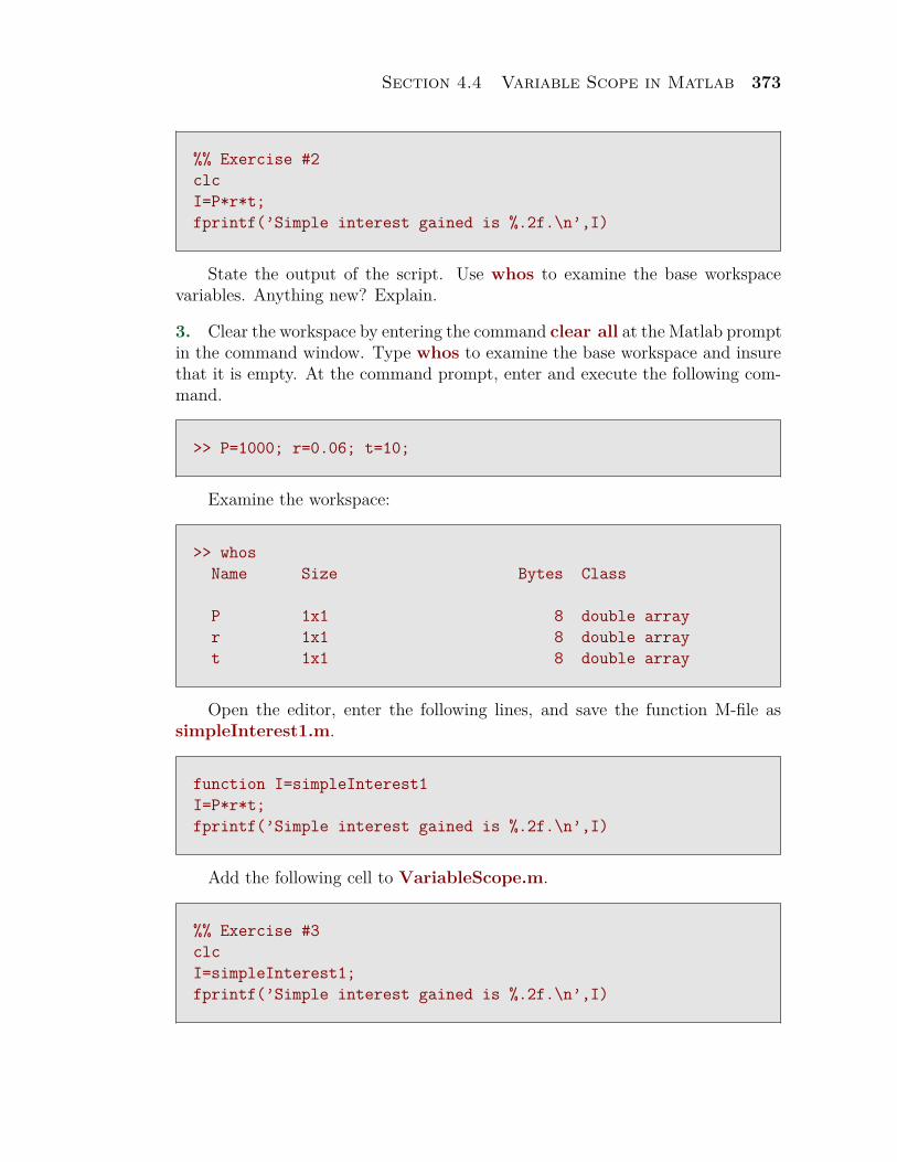
Section 4.4 Variable Scope in Matlab 373
%% Exercise #2clcI=P*r*t;fprintf(’Simple interest gained is %.2f.\n’,I)
State the output of the script. Use whos to examine the base workspacevariables. Anything new? Explain.
3. Clear the workspace by entering the command clear all at the Matlab promptin the command window. Type whos to examine the base workspace and insurethat it is empty. At the command prompt, enter and execute the following com-mand.
>> P=1000; r=0.06; t=10;
Examine the workspace:
>> whosName Size Bytes Class
P 1x1 8 double arrayr 1x1 8 double arrayt 1x1 8 double array
Open the editor, enter the following lines, and save the function M-file assimpleInterest1.m.
function I=simpleInterest1I=P*r*t;fprintf(’Simple interest gained is %.2f.\n’,I)
Add the following cell to VariableScope.m.
%% Exercise #3clcI=simpleInterest1;fprintf(’Simple interest gained is %.2f.\n’,I)
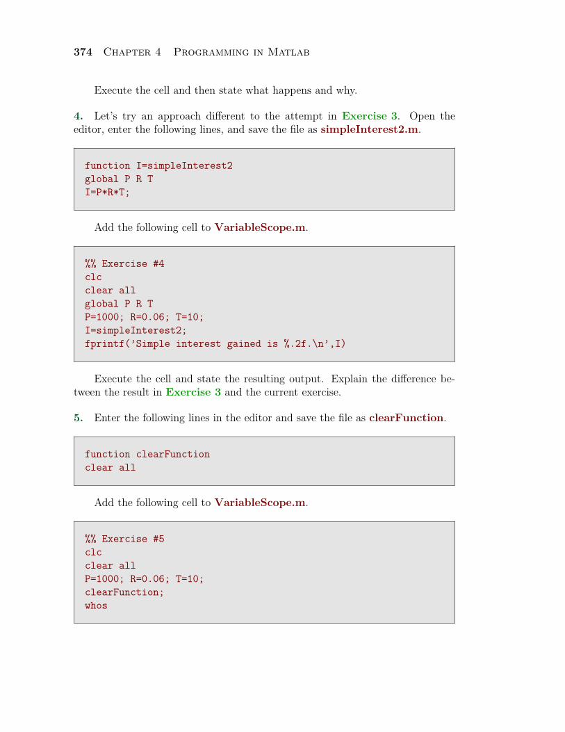
374 Chapter 4 Programming in Matlab
Execute the cell and then state what happens and why.
4. Let’s try an approach different to the attempt in Exercise 3. Open theeditor, enter the following lines, and save the file as simpleInterest2.m.
function I=simpleInterest2global P R TI=P*R*T;
Add the following cell to VariableScope.m.
%% Exercise #4clcclear allglobal P R TP=1000; R=0.06; T=10;I=simpleInterest2;fprintf(’Simple interest gained is %.2f.\n’,I)
Execute the cell and state the resulting output. Explain the difference be-tween the result in Exercise 3 and the current exercise.
5. Enter the following lines in the editor and save the file as clearFunction.
function clearFunctionclear all
Add the following cell to VariableScope.m.
%% Exercise #5clcclear allP=1000; R=0.06; T=10;clearFunction;whos
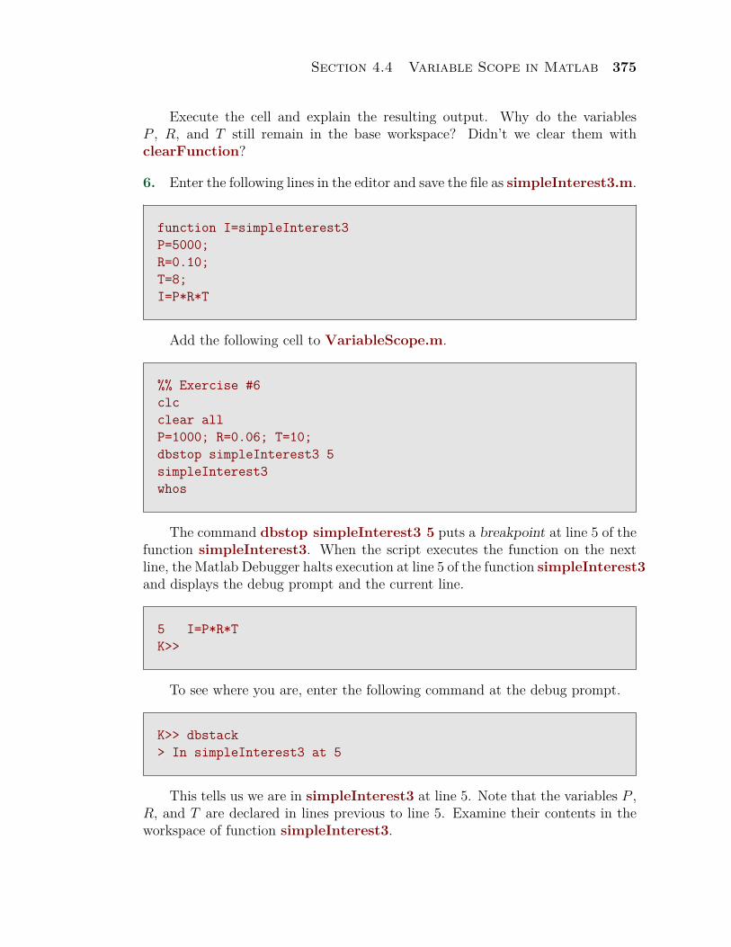
Section 4.4 Variable Scope in Matlab 375
Execute the cell and explain the resulting output. Why do the variablesP , R, and T still remain in the base workspace? Didn’t we clear them withclearFunction?
6. Enter the following lines in the editor and save the file as simpleInterest3.m.
function I=simpleInterest3P=5000;R=0.10;T=8;I=P*R*T
Add the following cell to VariableScope.m.
%% Exercise #6clcclear allP=1000; R=0.06; T=10;dbstop simpleInterest3 5simpleInterest3whos
The command dbstop simpleInterest3 5 puts a breakpoint at line 5 of thefunction simpleInterest3. When the script executes the function on the nextline, the Matlab Debugger halts execution at line 5 of the function simpleInterest3and displays the debug prompt and the current line.
5 I=P*R*TK>>
To see where you are, enter the following command at the debug prompt.
K>> dbstack> In simpleInterest3 at 5
This tells us we are in simpleInterest3 at line 5. Note that the variables P ,R, and T are declared in lines previous to line 5. Examine their contents in theworkspace of function simpleInterest3.
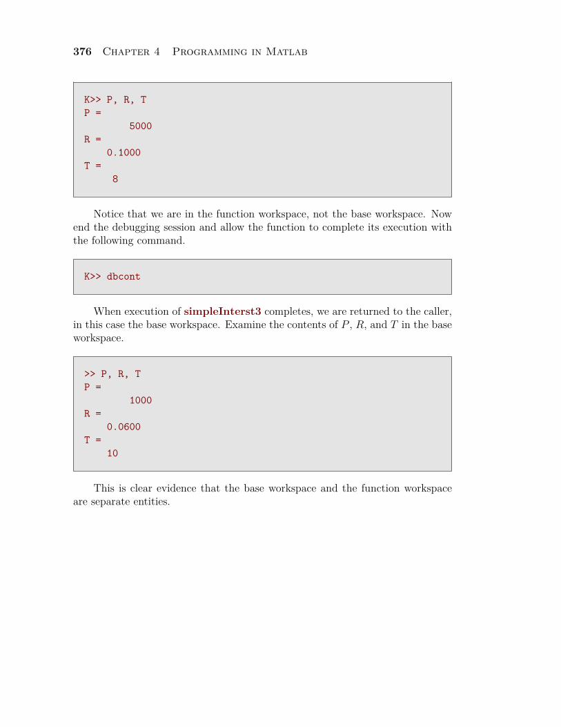
376 Chapter 4 Programming in Matlab
K>> P, R, TP =
5000R =
0.1000T =
8
Notice that we are in the function workspace, not the base workspace. Nowend the debugging session and allow the function to complete its execution withthe following command.
K>> dbcont
When execution of simpleInterst3 completes, we are returned to the caller,in this case the base workspace. Examine the contents of P , R, and T in the baseworkspace.
>> P, R, TP =
1000R =
0.0600T =
10
This is clear evidence that the base workspace and the function workspaceare separate entities.
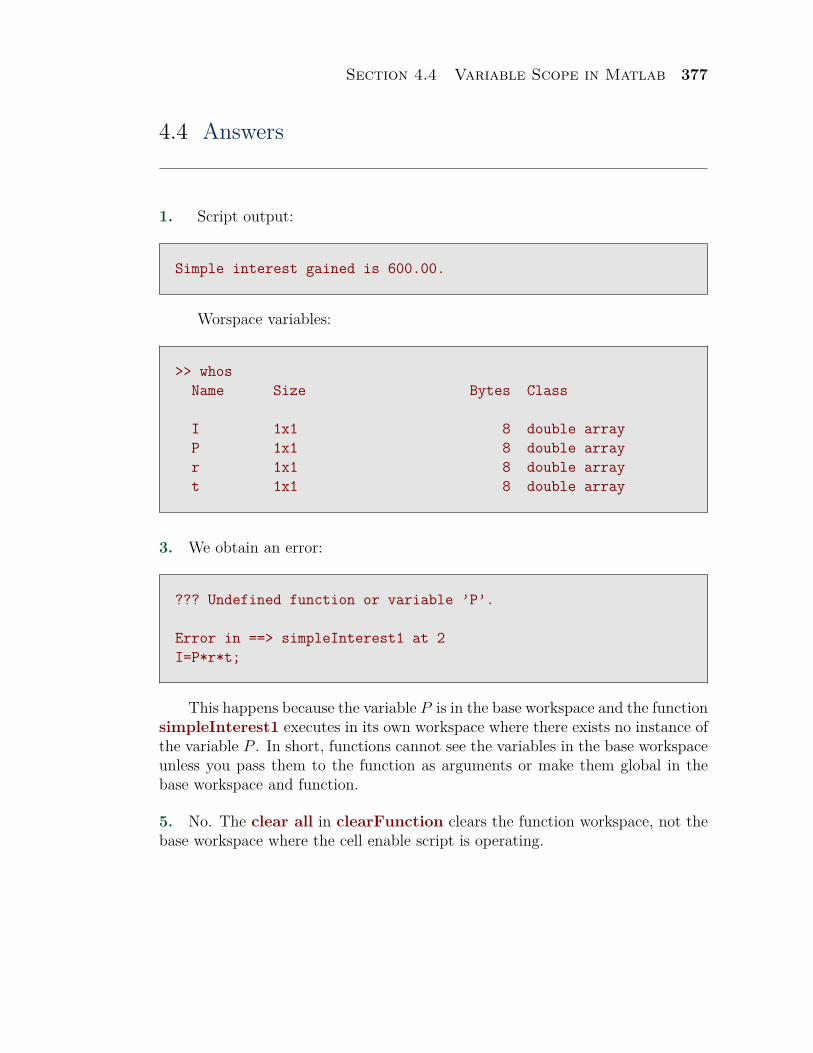
Section 4.4 Variable Scope in Matlab 377
4.4 Answers
1. Script output:
Simple interest gained is 600.00.
Worspace variables:
>> whosName Size Bytes Class
I 1x1 8 double arrayP 1x1 8 double arrayr 1x1 8 double arrayt 1x1 8 double array
3. We obtain an error:
??? Undefined function or variable ’P’.
Error in ==> simpleInterest1 at 2I=P*r*t;
This happens because the variable P is in the base workspace and the functionsimpleInterest1 executes in its own workspace where there exists no instance ofthe variable P . In short, functions cannot see the variables in the base workspaceunless you pass them to the function as arguments or make them global in thebase workspace and function.
5. No. The clear all in clearFunction clears the function workspace, not thebase workspace where the cell enable script is operating.

378 Chapter 4 Programming in Matlab
Section 4.5 Subfunctions in Matlab 379
4.5 Subfunctions in MatlabUp to this point, our programs have been fairly simple, usually taking on
a single task, such as solving a quadratic equation. As programs become morecomplex and perform multiple tasks, modern programmers break programs into aseries of self contained modules. In this manner, various parts of the program canbe written separately, tested, and once stable, can be integrated into the programas a whole.
In older programming languages, these modules were known as subroutines.In modern, object oriented languages such as C++ and Java, the modules areobjects, created from classes, that contain their own variables and methods formanipulating data and performing tasks. These objects can then be reused andassembled to create sophisticated programs.
To attack a complex programming task in Matlab, we must first break thetask up into manageable units. Each of these units or modules are then coded asfunctions and tested until we are certain they perform the simple task for whichthey are designed. Once satisfied that the individual functions are performing asdesigned, we must then integrate them into a complete and functioning program.
In this section we will discuss two ways that we can accomplish this modulardesign.
1. We can write each of the modules as functions in separate files. We then writea master script file which calls each of the function M-files as needed.
2. We can write a primary function in place of the script file. We can thenincorporate the modules as subfunctions directly in this primary function file.That is, we write one self contained file.
Actually there is also a third way to proceed. We can write a primary filein place of a script file. However, by signalling the end of this primary functionwith the Matlab keyword end, we signal Matlab that out subfunctions (each ofwhich must also use the keyword end) are nested functions. A primary functionwritten in this manner emulates some of the behavior of an object in an objectoriented language, with its own variables and methods (subfunctions). We’ll seein a later section that the rules for variable scope will change significantly whenusing nested functions.
We will investigate each of these options in some detail. In the next section,we investigate the first of these options, calling a function M-file from within thebody of a script M-file.
Copyrighted material. See: http://msenux.redwoods.edu/Math4Textbook/12
380 Chapter 4 Programming in Matlab
Calling Functions From Script FilesWe are going to tackle a programmng project that will perform rational arithmeticfor the user of the program. Options will include reducing, adding, subtracting,multiplying, and dividing fractions input by the user of our program.
Contemplating the design of such a program, here are some possible smallertasks that need implmentation.
1. Present the user with a menu of choices: reduction, addition, subtraction,multiplication, and division.
2. Routines will need to be written for each possible user choice on the menu.3. The program will need to query the user for a menu choice, then react in the
appropriate manner.
Note that this design is preliminary. In the process of writing a complexprogram, difficulties with the original design will surely arise. When that occurs,we will need to make modifications of the original design, which in turn will createthe need for design of new modules not considered in the first design.
However, one clear place that we can start is on the design of a menu ofchoices for the user of our program. Remember, the menu should query whataction the user wants to perform, reduction, addition, subtraction, or division.With this thought in mind, we write the following lines and save the script asrationalArithmetic.m.
clcfprintf(’Rational Arithmetic Menu:\n\n’)fprintf(’1). Reduce a fraction to lowest terms.\n’)fprintf(’2). Add two fractions.\n’)fprintf(’3). Subtract two fractions.\n’)fprintf(’4). Multiply two fractions.\n’)fprintf(’5). Divide two fractions.\n’)fprintf(’6). Exit program.\n\n’)n=input(’Enter number of your choice: ’);
Go to the Matlab prompt in the command window and execute the script bytyping the following.
>> rationalArithmetic
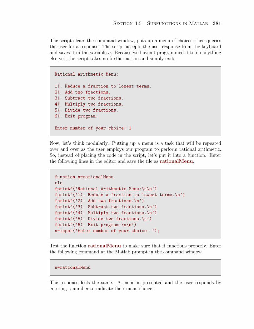
Section 4.5 Subfunctions in Matlab 381
The script clears the command window, puts up a menu of choices, then queriesthe user for a response. The script accepts the user response from the keyboardand saves it in the variable n. Because we haven’t programmed it to do anythingelse yet, the script takes no further action and simply exits.
Rational Arithmetic Menu:
1). Reduce a fraction to lowest terms.2). Add two fractions.3). Subtract two fractions.4). Multiply two fractions.5). Divide two fractions.6). Exit program.
Enter number of your choice: 1
Now, let’s think modularly. Putting up a menu is a task that will be repeatedover and over as the user employs our program to perform rational arithmetic.So, instead of placing the code in the script, let’s put it into a function. Enterthe following lines in the editor and save the file as rationalMenu.
function n=rationalMenuclcfprintf(’Rational Arithmetic Menu:\n\n’)fprintf(’1). Reduce a fraction to lowest terms.\n’)fprintf(’2). Add two fractions.\n’)fprintf(’3). Subtract two fractions.\n’)fprintf(’4). Multiply two fractions.\n’)fprintf(’5). Divide two fractions.\n’)fprintf(’6). Exit program.\n\n’)n=input(’Enter number of your choice: ’);
Test the function rationalMenu to make sure that it functions properly. Enterthe following command at the Matlab prompt in the command window.
n=rationalMenu
The response feels the same. A menu is presented and the user responds byentering a number to indicate their menu choice.
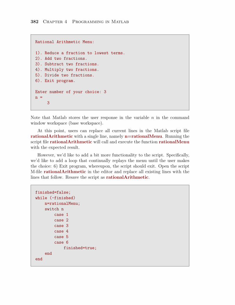
382 Chapter 4 Programming in Matlab
Rational Arithmetic Menu:
1). Reduce a fraction to lowest terms.2). Add two fractions.3). Subtract two fractions.4). Multiply two fractions.5). Divide two fractions.6). Exit program.
Enter number of your choice: 3n =
3
Note that Matlab stores the user response in the variable n in the commandwindow workspace (base workspace).
At this point, users can replace all current lines in the Matlab script filerationalArithmetic with a single line, namely n=rationalMenu. Running thescript file rationalArithmetic will call and execute the function rationalMenuwith the expected result.
However, we’d like to add a bit more functionality to the script. Specifically,we’d like to add a loop that continually replays the menu until the user makesthe choice: 6) Exit program, whereupon, the script should exit. Open the scriptM-file rationalArithmetic in the editor and replace all existing lines with thelines that follow. Resave the script as rationalArithmetic.
finished=false;while (~finished)
n=rationalMenu;switch n
case 1case 2case 3case 4case 5case 6
finished=true;end
end
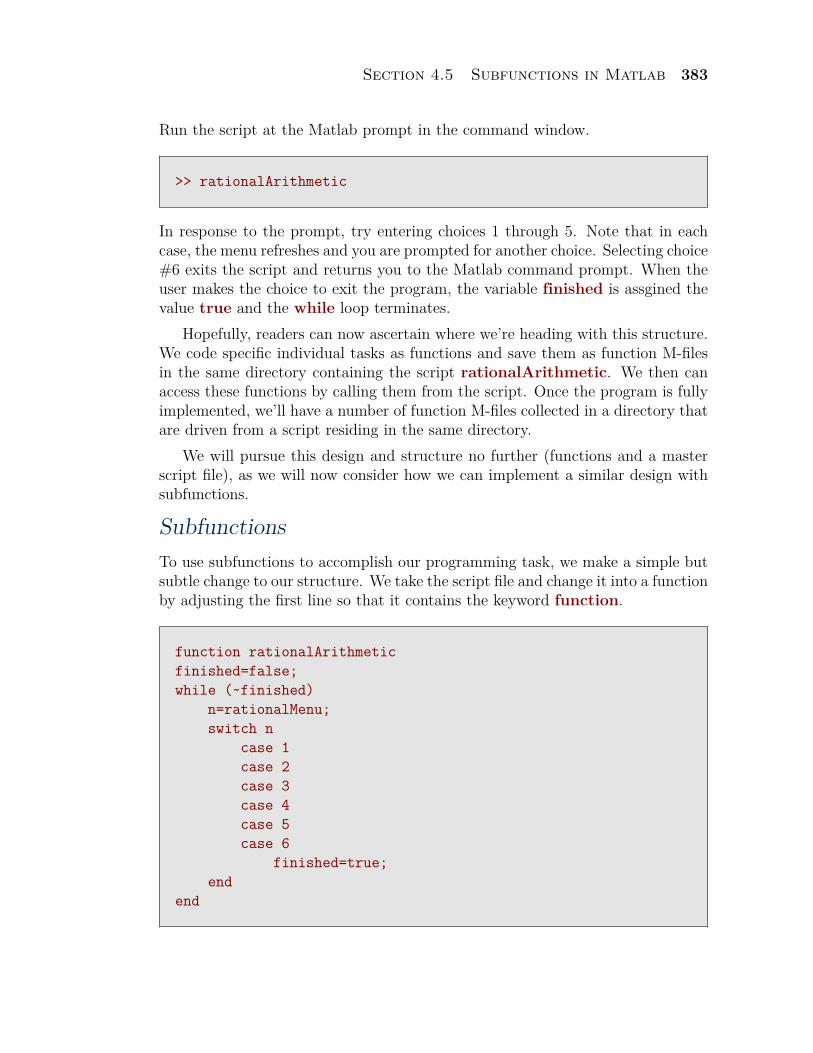
Section 4.5 Subfunctions in Matlab 383
Run the script at the Matlab prompt in the command window.
>> rationalArithmetic
In response to the prompt, try entering choices 1 through 5. Note that in eachcase, the menu refreshes and you are prompted for another choice. Selecting choice#6 exits the script and returns you to the Matlab command prompt. When theuser makes the choice to exit the program, the variable finished is assgined thevalue true and the while loop terminates.
Hopefully, readers can now ascertain where we’re heading with this structure.We code specific individual tasks as functions and save them as function M-filesin the same directory containing the script rationalArithmetic. We then canaccess these functions by calling them from the script. Once the program is fullyimplemented, we’ll have a number of function M-files collected in a directory thatare driven from a script residing in the same directory.
We will pursue this design and structure no further (functions and a masterscript file), as we will now consider how we can implement a similar design withsubfunctions.
SubfunctionsTo use subfunctions to accomplish our programming task, we make a simple butsubtle change to our structure. We take the script file and change it into a functionby adjusting the first line so that it contains the keyword function.
function rationalArithmeticfinished=false;while (~finished)
n=rationalMenu;switch n
case 1case 2case 3case 4case 5case 6
finished=true;end
end
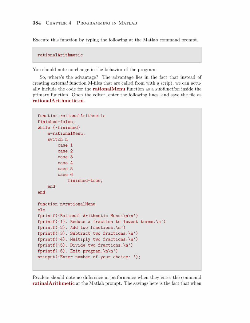
384 Chapter 4 Programming in Matlab
Execute this function by typing the following at the Matlab command prompt.
rationalArithmetic
You should note no change in the behavior of the program.So, where’s the advantage? The advantage lies in the fact that instead of
creating external function M-files that are called from with a script, we can actu-ally include the code for the rationalMenu function as a subfunction inside theprimary function. Open the editor, enter the following lines, and save the file asrationalArithmetic.m.
function rationalArithmeticfinished=false;while (~finished)
n=rationalMenu;switch n
case 1case 2case 3case 4case 5case 6
finished=true;end
end
function n=rationalMenuclcfprintf(’Rational Arithmetic Menu:\n\n’)fprintf(’1). Reduce a fraction to lowest terms.\n’)fprintf(’2). Add two fractions.\n’)fprintf(’3). Subtract two fractions.\n’)fprintf(’4). Multiply two fractions.\n’)fprintf(’5). Divide two fractions.\n’)fprintf(’6). Exit program.\n\n’)n=input(’Enter number of your choice: ’);
Readers should note no difference in performance when they enter the commandratinalArithmetic at the Matlab prompt. The savings here is the fact that when
Section 4.5 Subfunctions in Matlab 385
we replace the driving script file with a function M-file, this primary function cancontain as many subfunctions as needed to complete the programming task. Inthis way, the program is self contained. One file contains everything needed bythe program to perform the task for which it was designed.
Adding Functionality to our ProgramIn this section, we will write subfunctions that will reduce a fraction to lowestterms. This corresponds to the first choice on the menu of choices produced bythe subfunction rationalMenu.
How to proceed? We reduce a fraction to lowest terms in two steps. First, wefind a greatest common divisor for both numerator and denominator, then divideboth numerator and denominator by this greatest common denominator.
For example, to reduce the rational number 336/60 to lowest terms, we proceedas follows.
1. Find the greatest common divisior of 336 and 60, which is gcd(336, 60) = 12.2. Divide numerator and denominator by the greatest common divisor.
33660
= 336÷ 1260÷ 12
= 285
Two tasks call for two subfunctions, one to find the gcd and a second to dothe actual reduction.
The Euclidean Algorithm. Early in our mathematical education we learnthat if you take an nonegative integer a and divide it by a positive integer b, thereis an integer quotient q and remainder r such that
a = bq + r, 0 ≤ r < b.
We can use this Euclidean Algorithm to find the greatest common divisor of 336and 60. We proceed as follows.
1. When 376 is divided by 60, the quotient is 5 and the remainder is 36. That is,
336 = 5 · 60 + 36.
2. When 60 is divided by 36, the quotient is 1 and the remainder is 24. That is,
60 = 1 · 36 + 24.
3. When 36 is divided by 24, the quotient is 1 and the remainder is 12. That is,
36 = 1 · 24 + 12.
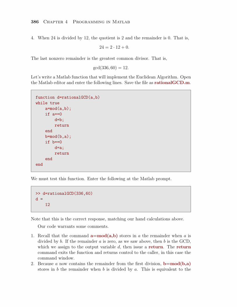
386 Chapter 4 Programming in Matlab
4. When 24 is divided by 12, the quotient is 2 and the remainder is 0. That is,
24 = 2 · 12 + 0.
The last nonzero remainder is the greatest common divisor. That is,
gcd(336, 60) = 12.
Let’s write a Matlab function that will implement the Euclidean Algorithm. Openthe Matlab editor and enter the following lines. Save the file as rationalGCD.m.
function d=rationalGCD(a,b)while true
a=mod(a,b);if a==0
d=b;return
endb=mod(b,a);if b==0
d=a;return
endend
We must test this function. Enter the following at the Matlab prompt.
>> d=rationalGCD(336,60)d =
12
Note that this is the correct response, matching our hand calculations above.Our code warrants some comments.
1. Recall that the command a=mod(a,b) stores in a the remainder when a isdivided by b. If the remainder a is zero, as we saw above, then b is the GCD,which we assign to the output variable d, then issue a return. The returncommand exits the function and returns control to the caller, in this case thecommand window.
2. Because a now contains the remainder from the first division, b=mod(b,a)stores in b the remainder when b is divided by a. This is equivalent to the
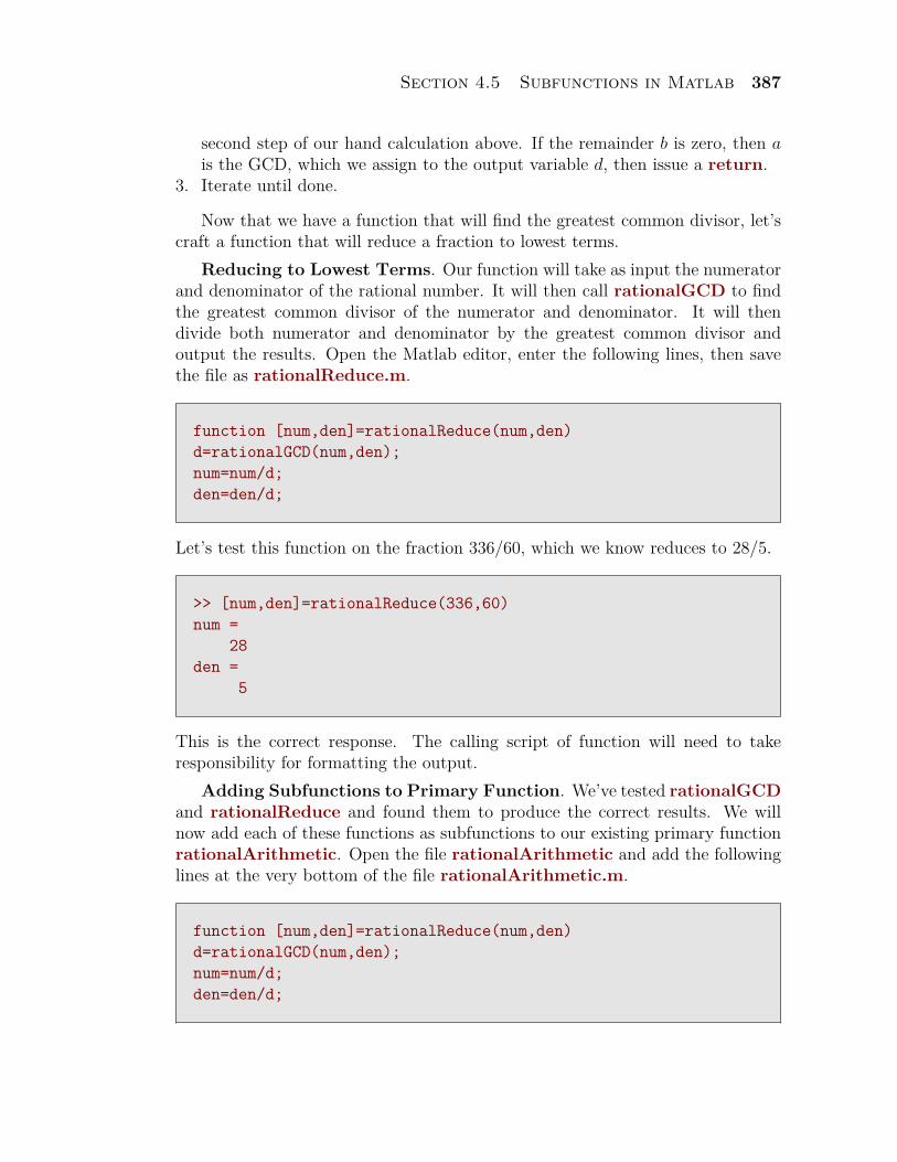
Section 4.5 Subfunctions in Matlab 387
second step of our hand calculation above. If the remainder b is zero, then ais the GCD, which we assign to the output variable d, then issue a return.
3. Iterate until done.
Now that we have a function that will find the greatest common divisor, let’scraft a function that will reduce a fraction to lowest terms.
Reducing to Lowest Terms. Our function will take as input the numeratorand denominator of the rational number. It will then call rationalGCD to findthe greatest common divisor of the numerator and denominator. It will thendivide both numerator and denominator by the greatest common divisor andoutput the results. Open the Matlab editor, enter the following lines, then savethe file as rationalReduce.m.
function [num,den]=rationalReduce(num,den)d=rationalGCD(num,den);num=num/d;den=den/d;
Let’s test this function on the fraction 336/60, which we know reduces to 28/5.
>> [num,den]=rationalReduce(336,60)num =
28den =
5
This is the correct response. The calling script of function will need to takeresponsibility for formatting the output.
Adding Subfunctions to Primary Function. We’ve tested rationalGCDand rationalReduce and found them to produce the correct results. We willnow add each of these functions as subfunctions to our existing primary functionrationalArithmetic. Open the file rationalArithmetic and add the followinglines at the very bottom of the file rationalArithmetic.m.
function [num,den]=rationalReduce(num,den)d=rationalGCD(num,den);num=num/d;den=den/d;
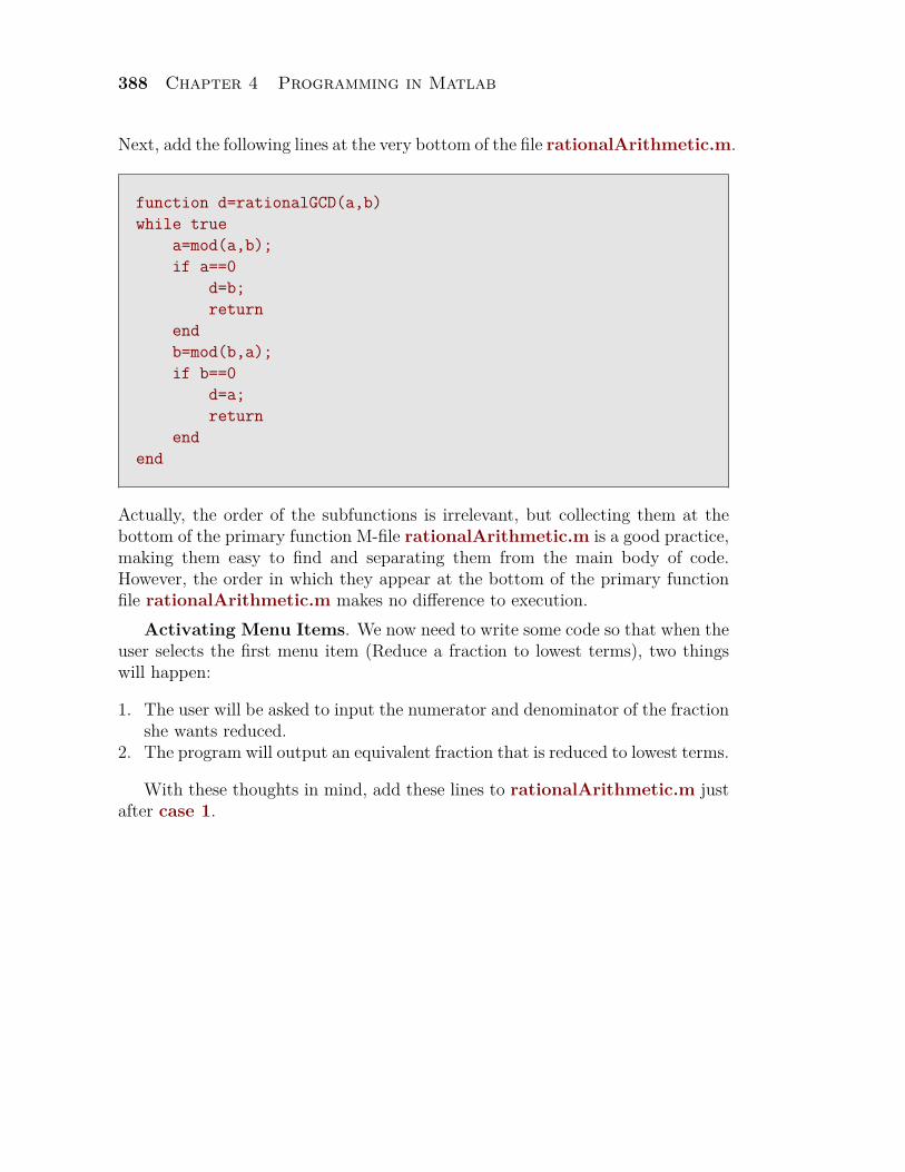
388 Chapter 4 Programming in Matlab
Next, add the following lines at the very bottom of the file rationalArithmetic.m.
function d=rationalGCD(a,b)while true
a=mod(a,b);if a==0
d=b;return
endb=mod(b,a);if b==0
d=a;return
endend
Actually, the order of the subfunctions is irrelevant, but collecting them at thebottom of the primary function M-file rationalArithmetic.m is a good practice,making them easy to find and separating them from the main body of code.However, the order in which they appear at the bottom of the primary functionfile rationalArithmetic.m makes no difference to execution.
Activating Menu Items. We now need to write some code so that when theuser selects the first menu item (Reduce a fraction to lowest terms), two thingswill happen:
1. The user will be asked to input the numerator and denominator of the fractionshe wants reduced.
2. The program will output an equivalent fraction that is reduced to lowest terms.
With these thoughts in mind, add these lines to rationalArithmetic.m justafter case 1.
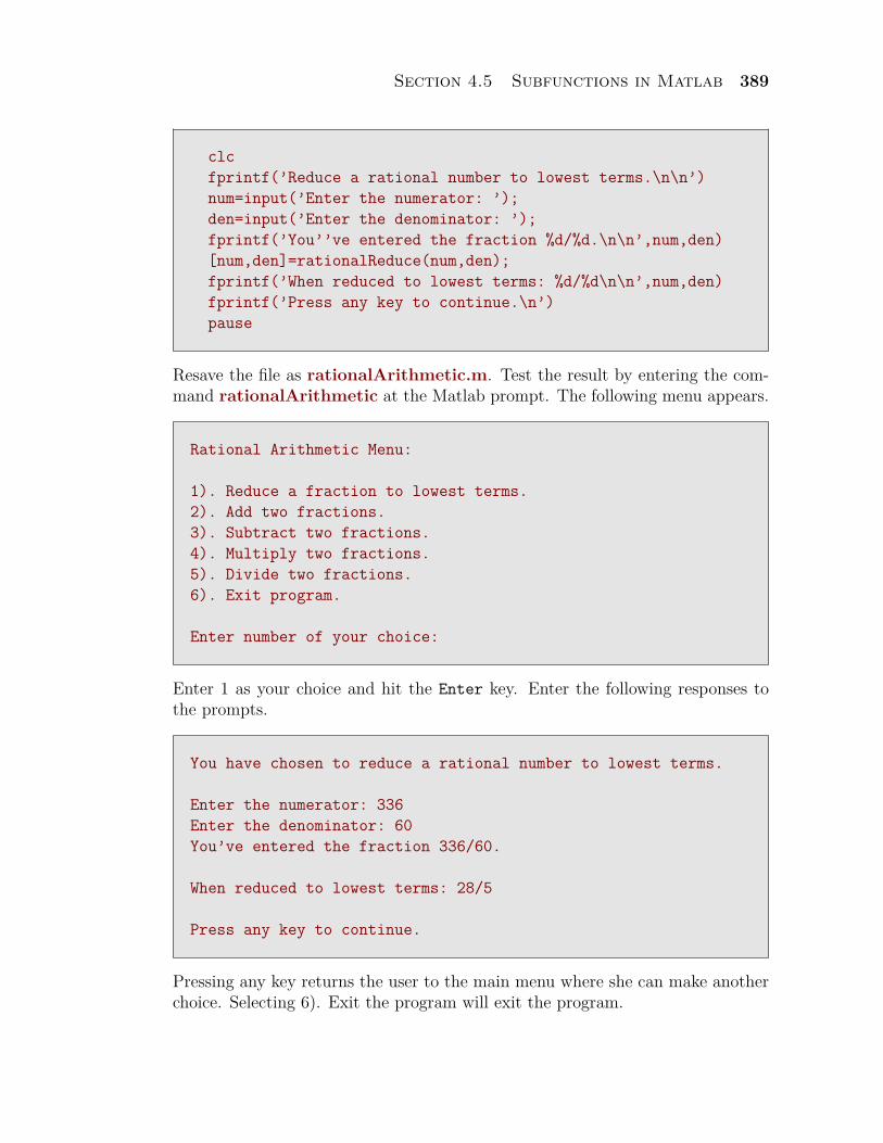
Section 4.5 Subfunctions in Matlab 389
clcfprintf(’Reduce a rational number to lowest terms.\n\n’)num=input(’Enter the numerator: ’);den=input(’Enter the denominator: ’);fprintf(’You’’ve entered the fraction %d/%d.\n\n’,num,den)[num,den]=rationalReduce(num,den);fprintf(’When reduced to lowest terms: %d/%d\n\n’,num,den)fprintf(’Press any key to continue.\n’)pause
Resave the file as rationalArithmetic.m. Test the result by entering the com-mand rationalArithmetic at the Matlab prompt. The following menu appears.
Rational Arithmetic Menu:
1). Reduce a fraction to lowest terms.2). Add two fractions.3). Subtract two fractions.4). Multiply two fractions.5). Divide two fractions.6). Exit program.
Enter number of your choice:
Enter 1 as your choice and hit the Enter key. Enter the following responses tothe prompts.
You have chosen to reduce a rational number to lowest terms.
Enter the numerator: 336Enter the denominator: 60You’ve entered the fraction 336/60.
When reduced to lowest terms: 28/5
Press any key to continue.
Pressing any key returns the user to the main menu where she can make anotherchoice. Selecting 6). Exit the program will exit the program.
390 Chapter 4 Programming in Matlab
A few comments are in order.
1. The fprintf commands are self explanatory.2. The heart of this code is the call to the rationalReduce subfunction, which
takes the user’s input for the numerator and denominator, then returns thereduced form of the numerator and denominator. The ensuing fprintf com-mands format the result.
3. The pause command is new, but simply explained. It halts program executionuntil the user strikes a key.
It should now be a simple matter to complete menu items #4 and #5. Youneed only multiply two rational numbers as follows,
a
b· c
d= a · c
b · d,
then reduce the result. For the division, you need only invert and multiply,a
b÷ c
d= a
b· d
c= a · d
b · c,
then reduce the result.To accomplish these tasks in code requires two subfunctions, rationalMultiply
and rationalDivide. You will also have to write code that requests input, per-forms the requested operation, then formats the output after case 4 and case5.
Addition and subtraction are a bit trickier.Finding a Least Common Denominator. To add and subtract fractions,
the program will need to find a least common denominator (LCD). For example,to add 5/12 and 3/8, we make equivalent fractions with a commond denominator,then add.
512
+ 38
= 1024
+ 924
= 1924
Additionally, you must insure that the answer is reduced to lowest terms.So, how do we write a subfunction that will produce a least common denomi-
nator? The following fact from number theory reveals the result.
lcd(a, b) = ab
gcd(a, b)
Thus,
lcd(8, 12) = 8 · 12gcd(8, 12)
= 964
= 24.
Section 4.5 Subfunctions in Matlab 391
Thus, the code for the least common denominator is clear. Open the editor andenter the following lines. Save the file as rationalLCD.m.
function m=rationalLCD(a,b)d=rationalGCD(a,b);m=(a*b)/d;
Test the result at the command line.
>> m=rationalLCD(8,12)m =
24
This is the correct response. Now copy the following lines and enter them at thebottom of the primary function rationalArithmetic.m as follows.
function m=rationalLCD(a,b)d=ratGCD(a,b);m=(a*b)/d;
Completing rationalArithmetic.mWe’ll leave it to our readers to complete the remaining tasks in the primaryfunction rationalArithmetic. Here is what remains to be done.
1. You’ll need to write subfunctions rationalAdd and rationalSubtract. Eachshould take two fractions as input, find an LCD, make equivalent fractions,add (or subtract), reduce, then send the result back to the caller.
2. Write code that requests input, performs the expected operation, then formatsthe output after case 2 and case 3.
Try to proceed as we have in the foregoing narrative. First write the standalonefunction rationalAdd. You might consider using the following first line.
function [num,den]=rationalAdd(num1,den1,num2,den2)
Note that the input calls for two fractions: num1 and den1 are the numeratorand denominator of the first fraction input by the user, num2 and den2 are
392 Chapter 4 Programming in Matlab
the numerator and denominator of the second fraction input by the user. Youwill want to make calls to rationalLCD and rationalReduce in the standalonefunction rationalAdd. Once you have the function rationalAdd tested andworking, paste it as a subfunction at the bottom of the file rationalArithmetic.
This is an imporant idea. Write the code for the smaller task. Test it thor-oughly. When you gain confidence in the result, then drop it in the larger programand coordinate it with the existing code.
Section 4.5 Subfunctions in Matlab 393
4.5 Exercises
1. Complete the program rationalArithmetic. Implement four subfunctions,rationalAdd, rationalSubtract, rationalMultiply and rationalDivide, thenadd code to the corresponding case structure that will prompt the user for in-put, call the appropriate subfunction, then format the output. Test your functionthoroughly.
2. Although Matlab handles the arithmetic of complex numbers quite nicely,in this exercise you will write your own function to perform complex arithmetic.First, a bit of review. Recall that i =
√−1 and i2 = −1. With these facts,
coupled with the knowledge that the usual laws of arithmetic apply equally wellto the complex numbers (commutative, associative, distributive, etc.), it is notdifficulty to show each of the following results.
i.) (a + bi) + (c + di) = (a + c) + (b + d)i
ii.) (a + bi)− (c + di) = (a + c)− (b + d)i
iii.) (a + bi)(c + di) = (ac− bd)− (ad + bc)i
iv.) a + bic + di
= (ac + bd) + (bc− ad)ic2 + d2
It is instructive to provide a proof of each of these results. Here is your task. Nameyour primary function complexArithmetic, then perform each of the followingtasks.
a.) Write a subfunction complexMenu that will offer the user a choice of fouroperations, addition, subtraction, multiplication, division, and exiting theprogram. This routine should ask the user for a numerical response andreturn the choice to the calling function in the output variable n.
b.) The primary function should have a case structure that responds to the user’schoice in n. Each item in the case structure should prompt the user to entertwo complex numbers as row vectors, i.e., as [a,b] and [c,d], representinga+bi and c+di, respectively. This input should be sent as row vectors to theappropriate subfunction, then the returned row vector should be formattedand printed to the screen with fprintf in a manner you deem fitting.
c.) Write four subfunctions, complexAdd, complexSubtract, complexMultiply,and complexDivide. Each subfunction should accept two row vectors as
Copyrighted material. See: http://msenux.redwoods.edu/IntAlgText/13
394 Chapter 4 Programming in Matlab
input and return a row vector as output. For example, the first line of thesubfunction complexDivide should read as follows.
function w=complexDivide(u,v)
Note that the function receives the row vectors [a, b] and [c, d] in the ar-guments u and v, respectively. The output of complexDivide should bereturned as a row vector in the output argument w. Before including yoursubfunction in the primary function, test it thoroughly. One suggestion wouldbe to turn on rational display with format rat, then enter (2+3i)/(2+i)at the Matlab prompt and note the result. Now, feed [2, 3] and [2, 1] to yourstandalone function complexDivide and compare the result. Once the sub-function is written and tested, add it as a subfunction to the primary functioncomplexArithmetic.
Thoroughly test the primary function complexArithmetic for accuracy, insur-ing that each of the five menu choices function properly and provide accurateoutput.
3. On November 13, 1843, Sir William Rowan Hamilton presented his first paperon the quaternions to the Royal Irish Academy. It was entitled On a new Species ofImaginary Quantities connected with a theory of Quaternions and was publishedin Volume 2 of the Proceedings of the Royal Irish Academy. It is interesting toread about the discovery in Sir William’s own words in a letter to his son.
Every morning in the early part of the above-cited month, on my comingdown to breakfast, your (then) little brother William Edwin, and yourself,used to ask me, “Well, Papa, can you multiply triplets”? Whereto I wasalways obliged to reply, with a sad shake of the head: “No, I can only addand subtract them.”But on the 16th day of the same month — which happened to be a Monday,and a Council day of the Royal Irish Academy — I was walking in to attendand preside, and your mother was walking with me, along the Royal Canal,to which she had perhaps driven; and although she talked with me nowand then, yet an under-current of thought was going on in my mind, whichgave at last a result, whereof it is not too much to say that I felt at oncethe importance. An electric circuit seemed to close; and a spark flashedforth, the herald (as I foresaw, immediately) of many long years to comeof definitely directed thought and work, by myself if spared, and at allevents on the part of others, if I should even be allowed to live long enoughdistinctly to communicate the discovery. Nor could I resist the impulse— unphilosophical as it may have been — to cut with a knife on a stone
Section 4.5 Subfunctions in Matlab 395
of Brougham Bridge, as we passed it, the fundamental formula with thesymbols, i, j, k; namely,
i2 = j2 = k2 = ijk = −1, (4.7)
which contains the Solution of the Problem, but of course, as an inscription,has long since mouldered away. A more durable notice remains, however,on the Council Books of the Academy for that day (October 16th, 1843),which records the fact, that I then asked for and obtained leave to read aPaper on Quaternions, at the First General Meeting of the session: whichreading took place accordingly, on Monday the 13th of the November fol-lowing.
This letter and other correspondence by Sir William, along with a collection ofhis work and papers, can be found at the following URL.
http://www.maths.tcd.ie/pub/HistMath/People/Hamilton/The quaternions grew out of Hamilton’s desire to extend the geometry associatedwith complex numbers. A complex number has the form a + bi, where a and bare arbitrary real numbers. Hamilton first attempted to extend this to anotherdimension, working with numbers having the triplet form a+bi+cj, but soon dis-coved that another dimension was needed. Thus, the general form of a quaternionis a + bi + cj + dk. The discovery of the relationship (4.7) initiated Hamilton’sjourney into the world of quaternions.To this day, the quaternions remain influential. Students in abstract algebra meetthe definition when they begin their work on the theory of groups. The geometryof quaternions enables rotations and reflections in four dimensional space. Therole of the quaternions in quantum mechanics and physics is nicely documentedat the following URL.
http://world.std.com/~sweetser/quaternions/qindex/qindex.htmlSir William had no difficulty determining how to add two quaternions. In short,
(a+bi+cj+dk)+(e+fi+gj+hk) = (a+e)+(b+f)i+(c+g)j+(d+h)k. (4.8)
The definition of subtraction established by Sir William is not unexpected.
(a+bi+cj+dk)−(e+fi+gj+hk) = (a−e)+(b−f)i+(c−g)j+(d−h)k (4.9)
Scalar multiplication was easily established by Sir William.
α(a + bi + cj + dk) = (αa) + (αb)i + (αc)j + (αd)k (4.10)
We now reach the point where Sir William was confounded, multiplication of twoquaternions. His startling breakthrough, captured during the walk with his wifealong the Royal Canal, allowed him to make the further developments.
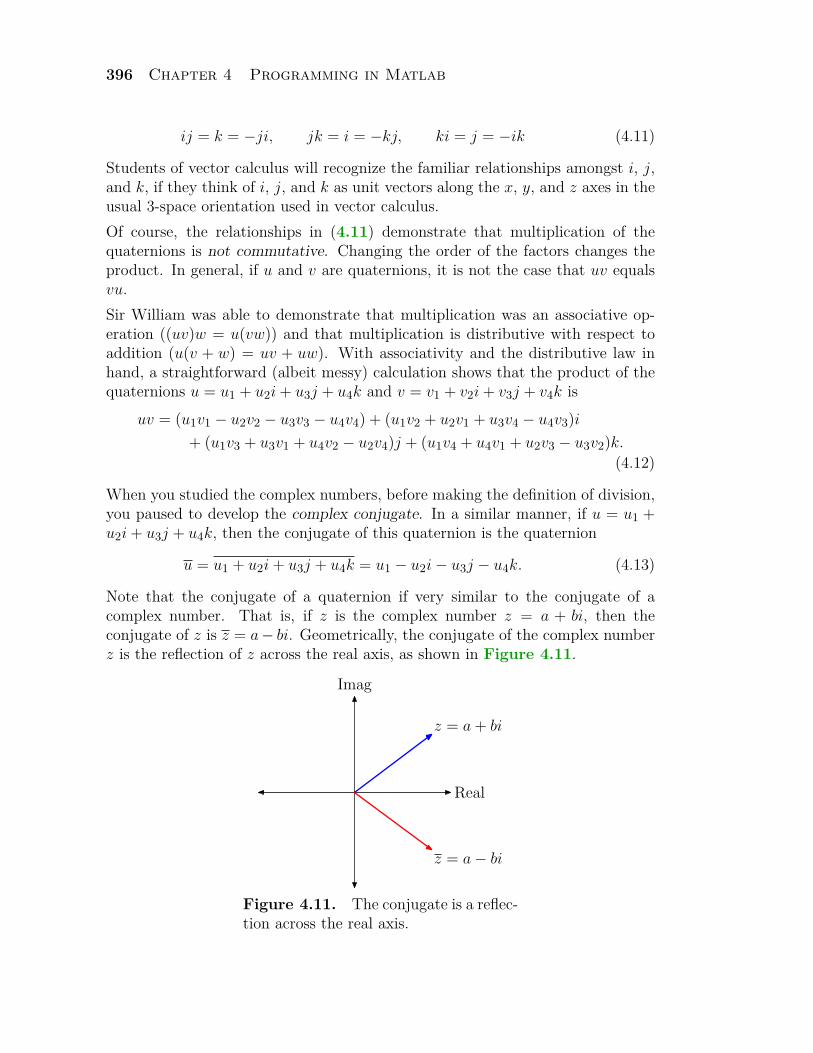
396 Chapter 4 Programming in Matlab
ij = k = −ji, jk = i = −kj, ki = j = −ik (4.11)
Students of vector calculus will recognize the familiar relationships amongst i, j,and k, if they think of i, j, and k as unit vectors along the x, y, and z axes in theusual 3-space orientation used in vector calculus.Of course, the relationships in (4.11) demonstrate that multiplication of thequaternions is not commutative. Changing the order of the factors changes theproduct. In general, if u and v are quaternions, it is not the case that uv equalsvu.Sir William was able to demonstrate that multiplication was an associative op-eration ((uv)w = u(vw)) and that multiplication is distributive with respect toaddition (u(v + w) = uv + uw). With associativity and the distributive law inhand, a straightforward (albeit messy) calculation shows that the product of thequaternions u = u1 + u2i + u3j + u4k and v = v1 + v2i + v3j + v4k is
uv = (u1v1 − u2v2 − u3v3 − u4v4) + (u1v2 + u2v1 + u3v4 − u4v3)i+ (u1v3 + u3v1 + u4v2 − u2v4)j + (u1v4 + u4v1 + u2v3 − u3v2)k.
(4.12)
When you studied the complex numbers, before making the definition of division,you paused to develop the complex conjugate. In a similar manner, if u = u1 +u2i + u3j + u4k, then the conjugate of this quaternion is the quaternion
u = u1 + u2i + u3j + u4k = u1 − u2i− u3j − u4k. (4.13)
Note that the conjugate of a quaternion if very similar to the conjugate of acomplex number. That is, if z is the complex number z = a + bi, then theconjugate of z is z = a− bi. Geometrically, the conjugate of the complex numberz is the reflection of z across the real axis, as shown in Figure 4.11.
Real
Imag
z = a + bi
z = a− bi
Figure 4.11. The conjugate is a reflec-tion across the real axis.
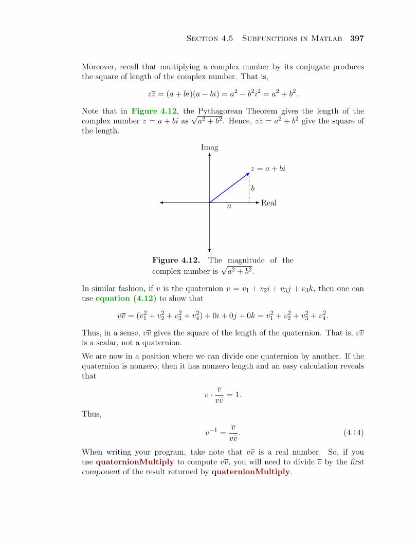
Section 4.5 Subfunctions in Matlab 397
Moreover, recall that multiplying a complex number by its conjugate producesthe square of length of the complex number. That is,
zz = (a + bi)(a− bi) = a2 − b2i2 = a2 + b2.
Note that in Figure 4.12, the Pythagorean Theorem gives the length of thecomplex number z = a + bi as
√a2 + b2. Hence, zz = a2 + b2 give the square of
the length.
Real
Imag
z = a + bi
a
b
Figure 4.12. The magnitude of thecomplex number is
√a2 + b2.
In similar fashion, if v is the quaternion v = v1 + v2i + v3j + v3k, then one canuse equation (4.12) to show that
vv = (v21 + v2
2 + v23 + v2
4) + 0i + 0j + 0k = v21 + v2
2 + v23 + v2
4.
Thus, in a sense, vv gives the square of the length of the quaternion. That is, vvis a scalar, not a quaternion.We are now in a position where we can divide one quaternion by another. If thequaternion is nonzero, then it has nonzero length and an easy calculation revealsthat
v · v
vv= 1.
Thus,
v−1 = v
vv. (4.14)
When writing your program, take note that vv is a real number. So, if youuse quaternionMultiply to compute vv, you will need to divide v by the firstcomponent of the result returned by quaternionMultiply.
398 Chapter 4 Programming in Matlab
Division is now easily defined.u
v= uv−1. (4.15)
We begin our programming task. Save a primary function as quaternionArithmetic,then perform each of the following tasks.
a.) The primary function should store the quaternions
u = 1 + 2i + 3j + 4k and v = 5 + 6i + 7j + 8k
as row vectors u=[1,2,3,4] and v=[5,6,7,8]. It should then use fprintf toformat and output four results to the screen, u + v, u− v, uv, and u/v.
b.) Write and implement each of the following subfunctions:
i.) function w=quaternionAdd(u,v)
ii.) function w=quaternionSubtract(u,v)
iii.) function v=quaternionConjugate(u)
iv.) fucntion v=quaternionInverse(u)
v.) function w=quaternionDivide(u,v)Note that the input and output to each of these routines are quaternions,which should be stored a row vectors of length four. Before adding eachsubfunction to your primary function, test each function thoroughly for ac-curacy.
Some hints are in order:
• quaternionAdd and quaternionSubtract should use equations (4.8) and4.9, respectively.
• quaternionMultiply should use equation (4.12).• quaternionConjugate should use equation (4.13).• quaternionInverse should use equation (4.14), which in turn requires a
call of the subfunction quaternionConjugate to complete the calculation.• quaternionDivide should use equation (4.15), which in turn will require
calls to quaternionInverse and quaternionMultiply to complete the cal-culation.
Because there is no user input involved, you should be able to open the editorin cell mode and simply call quaternionArithmetic and publish the result toHTML. Include your function quaternionArithmetic as a comment. Your gradeon this assignment will reflect the accuracy of your answers, so you might wantto compare and contrast your answers with your classmates. One way to do thisis through the Discussion Board on Blackboard.
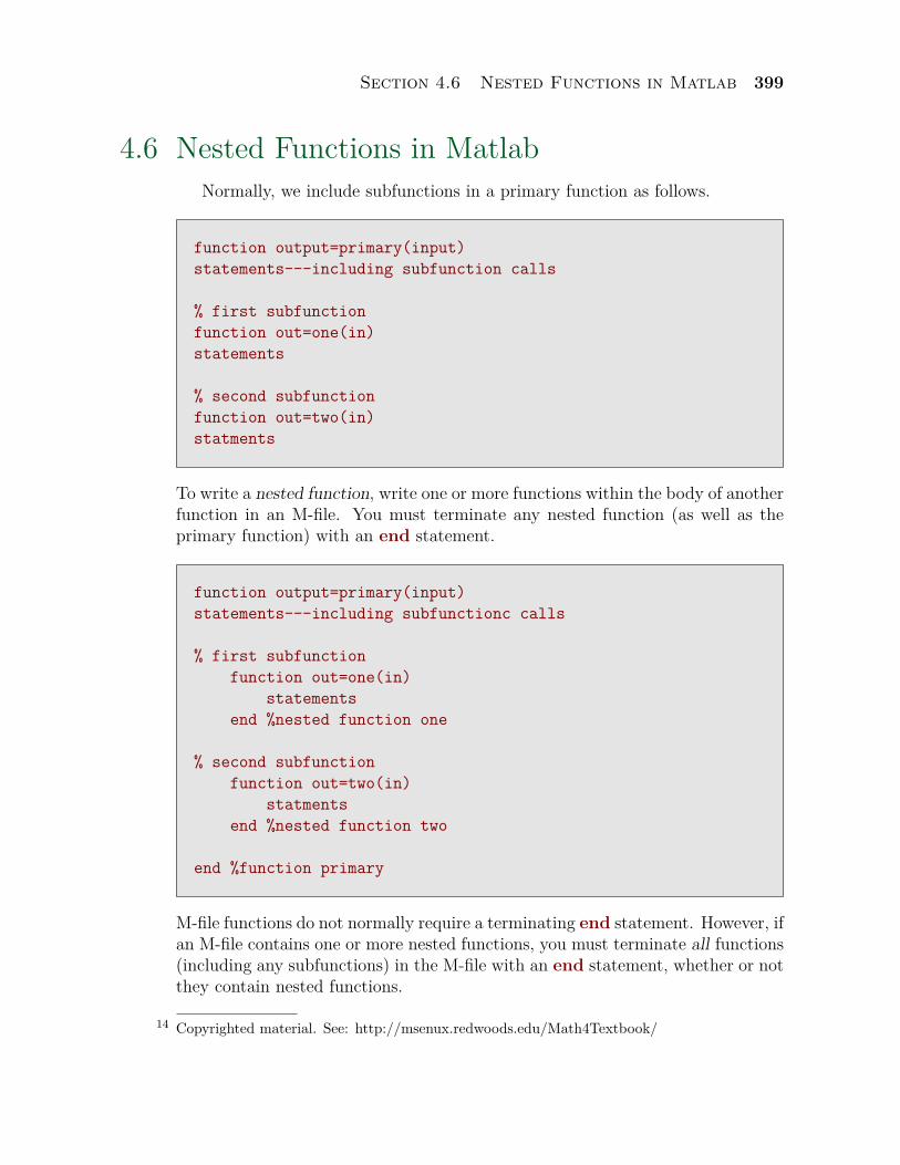
Section 4.6 Nested Functions in Matlab 399
4.6 Nested Functions in MatlabNormally, we include subfunctions in a primary function as follows.
function output=primary(input)statements---including subfunction calls
% first subfunctionfunction out=one(in)statements
% second subfunctionfunction out=two(in)statments
To write a nested function, write one or more functions within the body of anotherfunction in an M-file. You must terminate any nested function (as well as theprimary function) with an end statement.
function output=primary(input)statements---including subfunctionc calls
% first subfunctionfunction out=one(in)
statementsend %nested function one
% second subfunctionfunction out=two(in)
statmentsend %nested function two
end %function primary
M-file functions do not normally require a terminating end statement. However, ifan M-file contains one or more nested functions, you must terminate all functions(including any subfunctions) in the M-file with an end statement, whether or notthey contain nested functions.
Copyrighted material. See: http://msenux.redwoods.edu/Math4Textbook/14
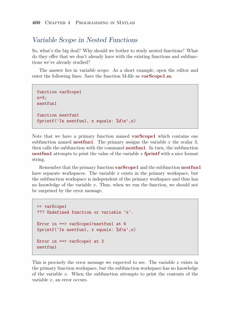
400 Chapter 4 Programming in Matlab
Variable Scope in Nested FunctionsSo, what’s the big deal? Why should we bother to study nested functions? Whatdo they offer that we don’t already have with the existing functions and subfunc-tions we’ve already studied?
The answer lies in variable scope. As a short example, open the editor andenter the following lines. Save the function M-file as varScope1.m.
function varScope1x=3;nestfun1
function nestfun1fprintf(’In nestfun1, x equals: %d\n’,x)
Note that we have a primary function named varScope1 which contains onesubfunction named nestfun1. The primary assigns the variable x the scalar 3,then calls the subfunction with the command nestfun1. In turn, the subfunctionnestfun1 attempts to print the value of the variable x fprintf with a nice formatstring.
Remember that the primary function varScope1 and the subfunction nestfun1have separate workspaces. The variable x exists in the primary workspace, butthe subfunction workspace is independent of the primary workspace and thus hasno knowledge of the variable x. Thus, when we run the function, we should notbe surprised by the error message.
>> varScope1??? Undefined function or variable ’x’.
Error in ==> varScope1>nestfun1 at 6fprintf(’In nestfun1, x equals: %d\n’,x)
Error in ==> varScope1 at 3nestfun1
This is precisely the error message we expected to see. The variable x exists inthe primary function workspace, but the subfunction workspace has no knowledgeof the variable x. When the subfunction attempts to print the contents of thevariable x, an error occurs.
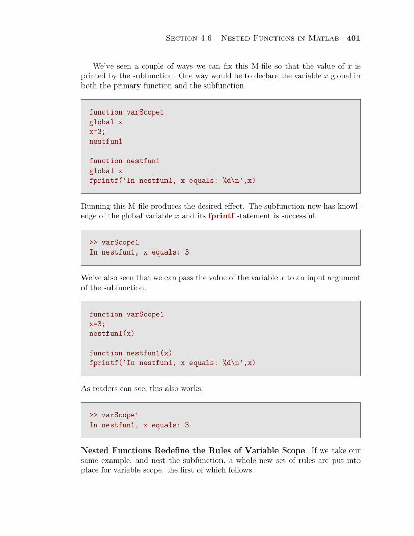
Section 4.6 Nested Functions in Matlab 401
We’ve seen a couple of ways we can fix this M-file so that the value of x isprinted by the subfunction. One way would be to declare the variable x global inboth the primary function and the subfunction.
function varScope1global xx=3;nestfun1
function nestfun1global xfprintf(’In nestfun1, x equals: %d\n’,x)
Running this M-file produces the desired effect. The subfunction now has knowl-edge of the global variable x and its fprintf statement is successful.
>> varScope1In nestfun1, x equals: 3
We’ve also seen that we can pass the value of the variable x to an input argumentof the subfunction.
function varScope1x=3;nestfun1(x)
function nestfun1(x)fprintf(’In nestfun1, x equals: %d\n’,x)
As readers can see, this also works.
>> varScope1In nestfun1, x equals: 3
Nested Functions Redefine the Rules of Variable Scope. If we take oursame example, and nest the subfunction, a whole new set of rules are put intoplace for variable scope, the first of which follows.
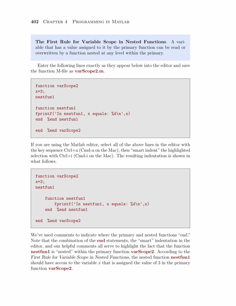
402 Chapter 4 Programming in Matlab
The First Rule for Variable Scope in Nested Functions. A vari-able that has a value assigned to it by the primary function can be read oroverwritten by a function nested at any level within the primary.
Enter the following lines exactly as they appear below into the editor and savethe function M-file as varScope2.m.
function varScope2x=3;nestfun1
function nestfun1fprintf(’In nestfun1, x equals: %d\n’,x)end %end nestfun1
end %end varScope2
If you are using the Matlab editor, select all of the above lines in the editor withthe key sequence Ctrl+a (Cmd-a on the Mac), then “smart indent” the highlightedselection with Ctrl+i (Cmd-i on the Mac). The resulting indentation is shown inwhat follows.
function varScope2x=3;nestfun1
function nestfun1fprintf(’In nestfun1, x equals: %d\n’,x)
end %end nestfun1
end %end varScope2
We’ve used comments to indicate where the primary and nested functions “end.”Note that the combination of the end statements, the “smart” indentation in theeditor, and our helpful comments all serve to highlight the fact that the functionnestfun1 is “nested” within the primary function varScope2. According to theFirst Rule for Variable Scope in Nested Functions, the nested function nestfun1should have access to the variable x that is assigned the value of 3 in the primaryfunction varScope2.
Section 4.6 Nested Functions in Matlab 403
>> varScope2In nestfun1, x equals: 3
Very interesting! No global variables, no passing of values as arguments, butbecause nestfun1 is “nested” within the primary function, the nested functionnestfun1 has access to all variables assigned in the primary function.
Graphical User InterfacesIn this section we introduce our readers to Matlab’s GUI’s Graphical User Inter-faces). Matlab has a full complement of uicontrols (User Interface Controls),typical of what you commonly see in most of today’s modern sofware: edit boxes,popupmenus, push- and toggle-buttons, sliders, radio buttons, and checkboxes, afew of which we will introduce in this section.
We’re going to write our first GUI, keeping it low-key as we introduce theconcepts. Our gui design can be described with the following series of tasks:
1. Plot a function.2. Provide radio buttons to change the color of the graph of the function, offering
choices of red, green, or blue.3. Provide a popup menu with choices of different line styles for the plot: solid,
dotted, etc.4. Provide an edit box that allows the user to change the linewidth.
Let’s begin. Open the editor and enter the following lines, then save thefunction M-file as plotGUI.m.
function plotGUI
close allclc
% plot domainxmin=0;xmax=4*pi;
% some colorsfigure_color=[0.8,0.9,0.8];panel_color=[1,0.9,0.8];buttongroup_color=[0.9,0.9,0.8];
404 Chapter 4 Programming in Matlab
This function takes no input and export no output. However, it is possible towrite GUI functions that accept input and export data back to the caller.
Next we close all open figure windows and clear the command window. Thisis helpful during the development of the GUI, but once we have a tested andworking program, we’ll remove these two commands from the GUI.
We set limits on the domain of our plot, which we will also use when weinitialize an axes on our figure window. It’s helpful to put these here and nothave to change them in several places in our program.
Finally, we initialize some colors we will use for our GUI components. Notethat each color takes the form of a row vector with three entries, each of whichmust be a number between 0 and 1. The first entry is the percentage of red,the second the percentage of green, and the third entry is the percentage of blue.Most modern computers have color wheels where you can view a color and thepercentages of red, green, and blue (in the RGB system) to make up the color.
Next, we’ll add a figure window to the GUI. Add the following lines to thefunction M-file plotGUI and save.
hFigure=figure(...’Units’,’Pixels’,...’Position’, [100 100 700 500],...’Color’,figure_color,...’MenuBar’,’none’,...’ToolBar’,’none’,...’NumberTitle’,’off’,...’Name’,’Plot GUI’);
Run the program. Some things to note:
1. We set Units to Pixels. Thereafter, all positioning commands are made inPixels. Think of a pixel as one dot on your computer screen. Typical resolutionon modern displays are of the order of 1024 by 768 pixels, but can be higher(or lower) depending on personal display settings on your computer.
2. Next we set the Position of the figure window at [100 100 700 500]. Thefirst two measurements (100 and 100) are the location of the lower left-handcorner of the figure window, relative to the lower left-hand corner of yourcomputer screen. The next two measurements (700 and 500) are the widthand height of the figure window. All of these measurements are in pixels
3. Finally, we set the color, then turn off the menubar and toolbar as well asthe usual number title that is displayed in a typical figure window (Figure 1,
Section 4.6 Nested Functions in Matlab 405
Figure 2, etc.). Then we give our figure window a meaningful name for theproject, namely Plot GUI.
4. Note that we assign a handle to the figure window named hFigure. EveryMatlab object can be associated with a handle for further reference.
We will now add an axes to the figure window. Note that the axes object willbe a “child” of the figure window (equivalently, the figure window is a “parent”of the axes object). Add the following lines to the file plotGUI and save.
hAxes=axes(...’Parent’,hFigure,...’Units’,’Pixels’,...’Position’,[50 50 400 400],...’Xlim’,[xmin,xmax],...’XGrid’,’on’,...’YGrid’,’on’);
Run the program. Things to note:
1. Note that the “Parent” of the axes object is set to hFigure, which is thenumerical handle assigned to the figure window designated above. This makesthe axes object a “child” of the figure window whose numerical handle ishFigure.
2. The unit of measurement for the axes object is also set to “Pixels.”3. The position of the axes object is set to [50 50 400 400]. The first two
numbers (50 and 50) set the lower left-hand corner of the axes object, relativeto the lower left-hand corner of its parent, in this case the figure windowdesignated by the handle hFigure.
4. The limits on the x-axis are set to [xmin,xmax] and the grid in both the x-and y-directions is turned ‘on’ (equivalent to using the grid on command).
5. Finally, note that we’ve assigned a handle hAxes to our axes object for furtherreference.
Now that we have a figure window and axes object, let’s create some data andplace a plot of the data on the axes object. Enter the following lines in plotGUIand save.
% plot datax=linspace(xmin,xmax);y=sin(2*x);hLine=line(x,y);
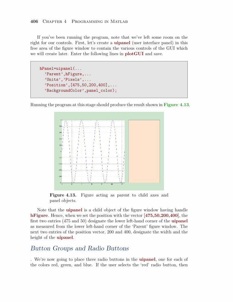
406 Chapter 4 Programming in Matlab
If you’ve been running the program, note that we’ve left some room on theright for our controls. First, let’s create a uipanel (user interface panel) in thisfree area of the figure window to contain the various controls of the GUI whichwe will create later. Enter the following lines in plotGUI and save.
hPanel=uipanel(...’Parent’,hFigure,...’Units’,’Pixels’,...’Position’,[475,50,200,400],...’BackgroundColor’,panel_color);
Running the program at this stage should produce the result shown in Figure 4.13.
Figure 4.13. Figure acting as parent to child axes andpanel objects.
Note that the uipanel is a child object of the figure window having handlehFigure. Hence, when we set the position with the vector [475,50,200,400], thefirst two entries (475 and 50) designate the lower left-hand corner of the uipanelas measured from the lower left-hand corner of the ‘Parent’ figure window. Thenext two entries of the position vector, 200 and 400, designate the width and theheight of the uipanel.
Button Groups and Radio Buttons. We’re now going to place three radio buttons in the uipanel, one for each ofthe colors red, green, and blue. If the user selects the ‘red’ radio button, then
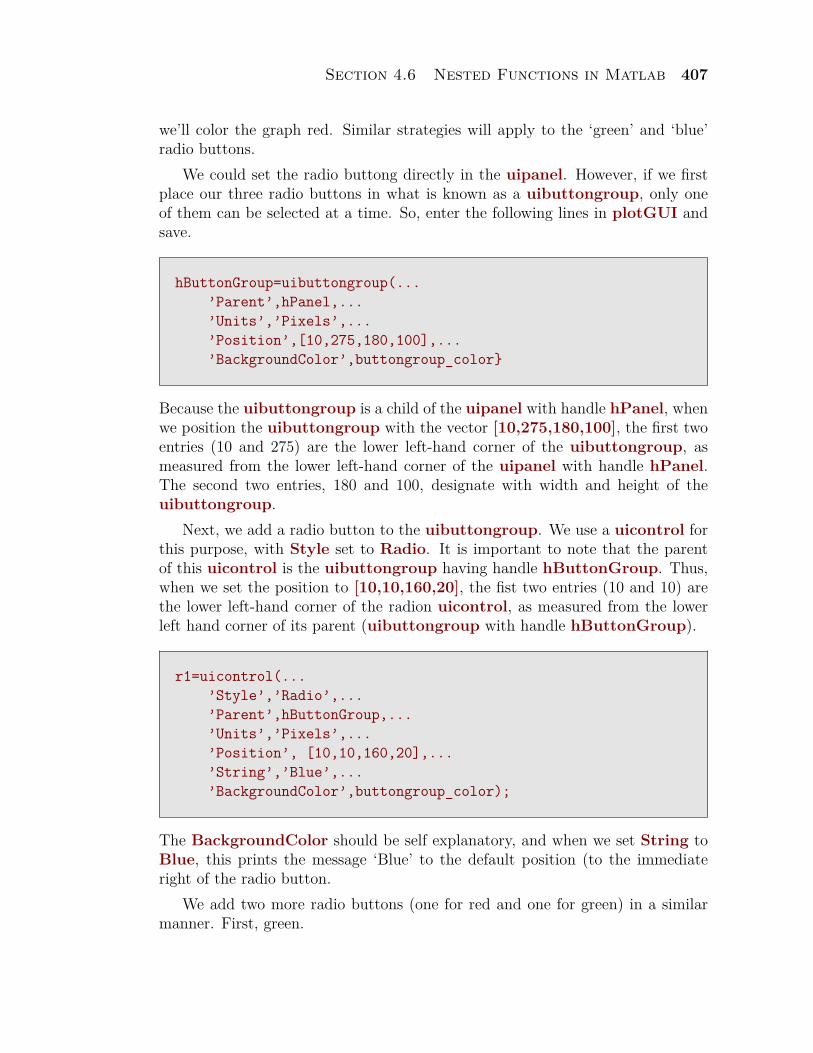
Section 4.6 Nested Functions in Matlab 407
we’ll color the graph red. Similar strategies will apply to the ‘green’ and ‘blue’radio buttons.
We could set the radio buttong directly in the uipanel. However, if we firstplace our three radio buttons in what is known as a uibuttongroup, only oneof them can be selected at a time. So, enter the following lines in plotGUI andsave.
hButtonGroup=uibuttongroup(...’Parent’,hPanel,...’Units’,’Pixels’,...’Position’,[10,275,180,100],...’BackgroundColor’,buttongroup_color}
Because the uibuttongroup is a child of the uipanel with handle hPanel, whenwe position the uibuttongroup with the vector [10,275,180,100], the first twoentries (10 and 275) are the lower left-hand corner of the uibuttongroup, asmeasured from the lower left-hand corner of the uipanel with handle hPanel.The second two entries, 180 and 100, designate with width and height of theuibuttongroup.
Next, we add a radio button to the uibuttongroup. We use a uicontrol forthis purpose, with Style set to Radio. It is important to note that the parentof this uicontrol is the uibuttongroup having handle hButtonGroup. Thus,when we set the position to [10,10,160,20], the fist two entries (10 and 10) arethe lower left-hand corner of the radion uicontrol, as measured from the lowerleft hand corner of its parent (uibuttongroup with handle hButtonGroup).
r1=uicontrol(...’Style’,’Radio’,...’Parent’,hButtonGroup,...’Units’,’Pixels’,...’Position’, [10,10,160,20],...’String’,’Blue’,...’BackgroundColor’,buttongroup_color);
The BackgroundColor should be self explanatory, and when we set String toBlue, this prints the message ‘Blue’ to the default position (to the immediateright of the radio button.
We add two more radio buttons (one for red and one for green) in a similarmanner. First, green.
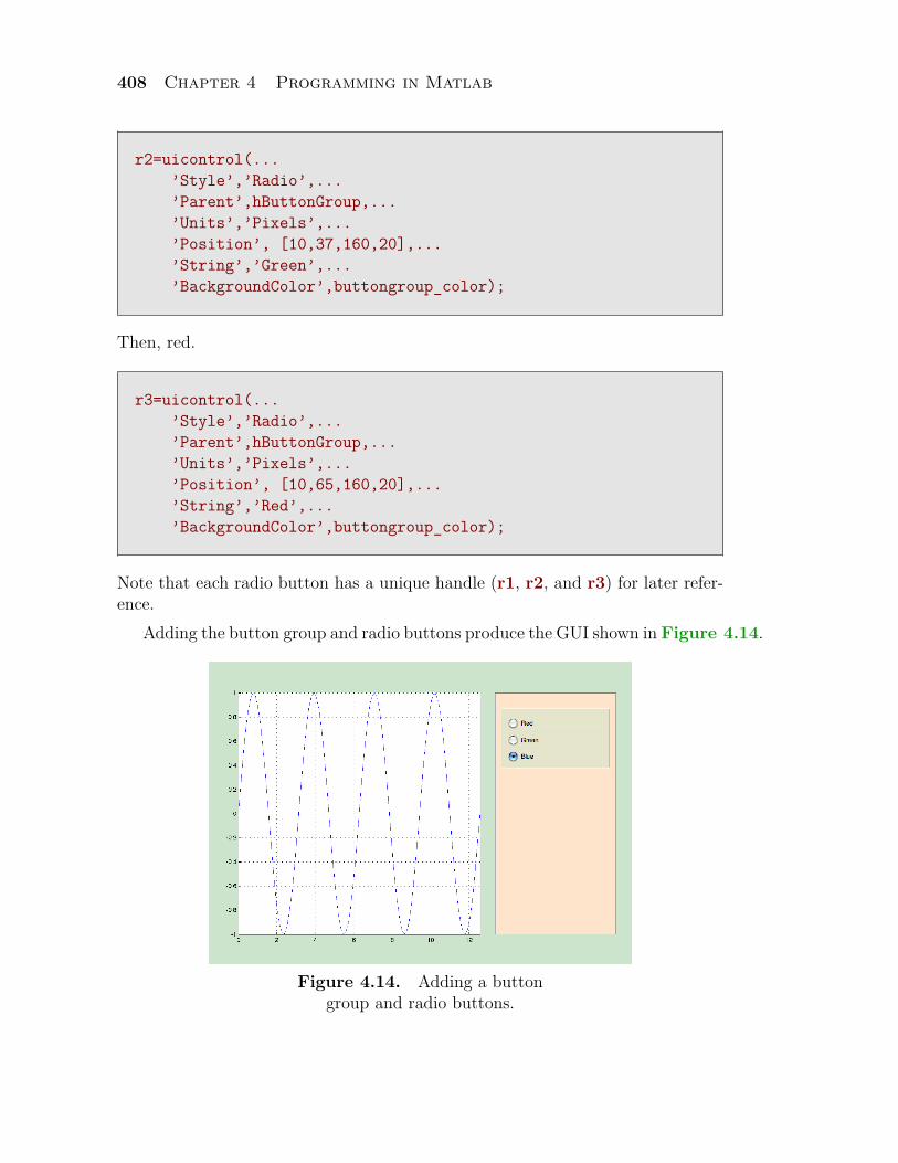
408 Chapter 4 Programming in Matlab
r2=uicontrol(...’Style’,’Radio’,...’Parent’,hButtonGroup,...’Units’,’Pixels’,...’Position’, [10,37,160,20],...’String’,’Green’,...’BackgroundColor’,buttongroup_color);
Then, red.
r3=uicontrol(...’Style’,’Radio’,...’Parent’,hButtonGroup,...’Units’,’Pixels’,...’Position’, [10,65,160,20],...’String’,’Red’,...’BackgroundColor’,buttongroup_color);
Note that each radio button has a unique handle (r1, r2, and r3) for later refer-ence.
Adding the button group and radio buttons produce the GUI shown in Figure 4.14.
Figure 4.14. Adding a buttongroup and radio buttons.
Section 4.6 Nested Functions in Matlab 409
At this point, you can try clicking each of the radio buttons, red, blue, or green.Although they are not programmed to do anything at this point, note that onlyone of them can be selected at a time. This behavior (one at a time selection) isdue to the fact that we grouped them inside a uibuttongroup.
Adding a Function Callback to the UIButtonGroupNote that the handle hButtonGroup can be used to get or set property-valuepairs for the uibuttongroup. You can obtain information on all possible property-value pairs for a uibuttongroup by typing doc uibuttongroup at the Matlabprompt. We are particularly interested in the SelectionChangeFcn property,to which we must assign a handle to a function. This sort of function is referredto as a callback function and will be executed whenever a new radio button isselected with the mouse. (Hence the property name, SelectionChangeFcn). Itdoesn’t matter what name you use for the callback function, but writers of MatlabGUI’s tend to use a descriptive name that includes the substring ‘callback.’ Thus,we’ll name the callback colorSelection_callback.
Add one more property-value pair to the uibuttongroup as follows.
hButtonGroup=uibuttongroup(...’Parent’,hPanel,...’Units’,’Pixels’,...’Position’,[10,275,180,100],...’BackgroundColor’,buttongroup_color,...’SelectionChangeFcn’,@colorSelection_callback);
Note that this is not new code. We simply appended the last property-value pairto the existing code that initialized the uibuttongroup.
Now, whenever you click a radio button with your mouse, the callback functionnamed colorSelection_callback will be executed. You can give it a try at thispoint, but the callback function does not yet exist in our GUI code, so you willreceive an error message attesting to that fact.
What we need to do next is write the function callback. So, go to the end of thefile plotGUI.m, just prior to the closing end of the primary function plotGUI,and add the following lines. We’ll fill in the body of this function callback in amoment, but just add these lines at present.
function colorSelection_callback(hObject,eventdata)end % end colorSelection_callback
410 Chapter 4 Programming in Matlab
Note that this callback function is nested inside the primary function plotGUI.Note the end command, which you must use to terminate any nested function.
Some comments are in order.
• The name of the callback must match the name of the function handle assignedto the property SelectionChangeFcn in the uibuttongroup.
• Two input arguments are required. You may use any names you wish.i. The first argument, which we have named hObject, receives the value of
the handle of the calling object. In this case, hObject receives the handleof the uibuttongroup, namely hButtonGroup.
ii. The second argument, which we have named eventdata, is passed a struc-ture containing data describing the state of the calling object when trig-gered by an event (in this case the clicking of a radio button by themouse). In this case, the structure eventdata contains two fields, onenamed OldValue, which contains the handle of the previously selectedradio button, and a second named NewValue, which contains the handleof the newly selected radio button. Note that the possible handles con-tained in these fields are three: r1, r2, or r3. You can access the value ofthese fields by typing the structure name, a period, then the field desired.For example, to get the handle to the newly selected radion button, typeeventdata.NewValue. To get the handle of the previously selected radiobutton, type eventdata.OldValue.
We’ll now code the body of the callback function. First, we get the value ofthe currently selected radio button and query the handle for the value of ‘String,’which could be either ‘Red’, ‘Green’, or ‘Blue’ (see the initialization strings foreach radio button described and coded earlier). We set up a switch structure,which will color the plot red, green, or blue, depending on whether lineColorequals ‘Red’, ‘Green’, or ‘Blue’.
function colorSelection_callback(hObject,eventdata)lineColor=get(eventdata.NewValue, ’String’);switch lineColor
case ’Red’set(hLine,’Color’,’r’)
case ’Green’set(hLine,’Color’,’g’)
case ’Blue’set(hLine,’Color’,’b’)
endend % end colorSelection_callback
Section 4.6 Nested Functions in Matlab 411
The thing to note is the fact that the nested callback has access to all variablesdefined in the outer primary function. In particular, hLine is a handle to thesinusoidal plot and it was defined in the primary function. Hence, the nestedfunction colorSelect_callback has access to this variable by default. It is notnecessary to pass the variable by value or to declare it global. Note that in eachcase of the switch structure, the code uses the handle hLine to set the ‘Color’property of the plot to the appropriate color.
At this point, you should be able to run the function without error. The GUIwill initialize, after which you can click the radio buttons and watch the plotchange to the color associated with the selected radio button.
Popup MenusIn this section we will add a popup menu containing choices of line styles forour plot. However, before adding the popup uicontrol, we will first add someexplanatory text by adding a uicontrol containing static text. Static text is notdynamic15, as the name implies, and is used specifically to annotate your GUIwith help messages and instructions.
So, immediately following the code for your last radio button (the code withhandle r3), enter the following lines.
hLineStyleText=uicontrol(...’Style’,’text’,...’Parent’,hPanel,...’Position’, [10 240 180 20],...’String’, ’LineStyle Choices’,...’HorizontalAlignment’,’Left’,...’BackgroundColor’, panel_color);
Again, comments are in order.
• The ‘Style’ of the uicontrol is ’text’. This declares the control as static text.The text that is actually printed on your GUI is the value of the ‘String’property, in this case “LineStyle Choices.” Underneath this static text, wewill soon place a popup menu with choices for line styles.
• Not that this uicontrol is a child of the uipanel with handle hPanel. Con-sequently, any positioning is measured from the lower left-hand corner of theuipanel.
Although static text cannot be modified by the user, it can be modified by the program code.15
412 Chapter 4 Programming in Matlab
Next, we deal with the popup menu. Following the code for our static text,enter these lines to intialize a popup menu of line style choices.
hLineStylePopup=uicontrol(...’Style’,’popup’,...’Parent’,hPanel,...’Units’,’Pixels’,...’Position’, [10 225 180 15],...’String’,{’Solid’ ’Dotted’ ’DashDot’ ’Dashed’ ’None’},...’BackgroundColor’, buttongroup_color,...’Callback’, @LineStylePopup_callback);
Here are a few words of explanation. First, some simple comments.
• The ‘Style’ of the uicontrol is ’popup’. This declares the control to be apopup menu.
• Again, the ’Parent’ of this uicontrol is the uipanel with handle hPanel.Thus, the position is again measured from the lower left=hand corner of theuipanel.
The ‘String’ property of the uicontrol is a cell containing the individualstrings that we wish to appear on the popup menu. A cell is a Matlab datastructure that allows the user to collect different data types in a set.
One of the simplest ways to build a cell in Matlab is shown in the code thatfollows. You should enter this code at the Matlab prompt, not in the code of ourGUI that is under construction.
>> C={’dashed’, 1:5, magic(3)}C =
’dashed’ [1x5 double] [3x3 double]
Note that we have collected three different data types in a cell, delimiting theentries with curly braces, and assigned the result to the variable C. The firstentry is a string, the second a row vector, and the third a 3× 3 matrix.
You can access the contents of the individual elements of a cell by using curlybraces with the usual indexing. For example, to obtain the contents of the firstentry in C, enter the following code (again, at the Matlab prompt, not in thecode for the GUI).
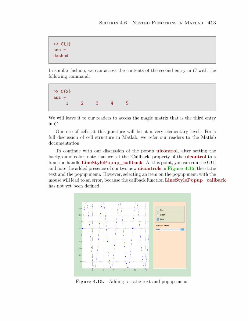
Section 4.6 Nested Functions in Matlab 413
>> C{1}ans =dashed
In similar fashion, we can access the contents of the second entry in C with thefollowing command.
>> C{2}ans =
1 2 3 4 5
We will leave it to our readers to access the magic matrix that is the third entryin C.
Our use of cells at this juncture will be at a very elementary level. For afull discussion of cell structure in Matlab, we refer our readers to the Matlabdocumentation.
To continue with our discussion of the popup uicontrol, after setting thebackground color, note that we set the ‘Callback’ property of the uicontrol to afunction handle LineStylePopup_callback. At this point, you can run the GUIand note the added presence of our two new uicontrols in Figure 4.15, the statictext and the popup menu. However, selecting an item on the popup menu with themouse will lead to an error, because the callback function LineStylePopup_callbackhas not yet been defined.
Figure 4.15. Adding a static text and popup menu.
414 Chapter 4 Programming in Matlab
So, let’s defined the callback for the popup menu of line styles. Just below thecallback function colorSelection_callback, add the following lines.
function LineStylePopup_callback(hObject,eventdata)lineStyleChoices=get(hObject,’String’);lineStyleChoice=get(hObject,’Value’);lineStyle=lineStyleChoices{lineStyleChoice};switch lineStyle
case ’Solid’set(hLine,’LineStyle’,’-’)
case ’Dotted’set(hLine,’LineStyle’,’:’)
case ’DashDot’set(hLine,’LineStyle’,’-.’)
case ’Dashed’set(hLine,’LineStyle’,’--’)
case ’None’set(hLine,’LineStyle’,’none’)
endend % end LineStylePopup_callback
We will make several comments regarding this callback.
• The first line contains the function keyword and the name of the callback, inthis case LineStylePopup_callback. The descriptive name of this callbackis a reminder of it is designed to provide. Note the oblibatory arguments,hObject and eventdata. The argument hObject will receive the handle ofthe calling object (in this case, the handle of the popup menu uicontrol). Inthis example, the argument eventdata is not used, but it is still required. Asmore evolutions of Matlab are updated, plans are in the works to make moreuse of the argument eventdata (as we did with our uibuttongroup, but forthe meantime, it’s not used in this callback, but it is still required.
• Because hObject is passed the handle to the popup uicontrol, we can use itto access two properties of that control, the ‘String’ and ‘Value’ properties.i. The ‘String’ property contains a cell of strings, each of which describe a
line style.ii. The ‘Value’ property contains a number indicating which entry on the
popup menu was selected by the user.
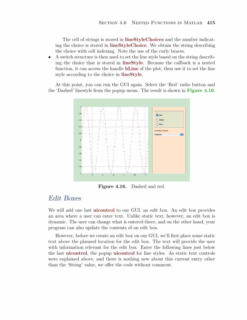
Section 4.6 Nested Functions in Matlab 415
The cell of strings is stored in lineStyleChoices and the number indicat-ing the choice is stored in lineStyleChoice. We obtain the string describingthe choice with cell indexing. Note the use of the curly braces.
• A switch structure is then used to set the line style based on the string describ-ing the choice that is stored in lineStyle. Because the callback is a nestedfunction, it can access the handle hLine of the plot, then use it to set the linestyle according to the choice in lineStyle.
At this point, you can run the GUI again. Select the ‘Red’ radio button andthe ‘Dashed’ linestyle from the popup menu. The result is shown in Figure 4.16.
Figure 4.16. Dashed and red.
Edit BoxesWe will add one last uicontrol to our GUI, an edit box. An edit box providesan area where a user can enter text. Unlike static text, however, an edit box isdynamic. The user can change what is entered there, and on the other hand, yourprogram can also update the contents of an edit box.
However, before we create an edit box on our GUI, we’ll first place some statictext above the planned location for the edit box. The text will provide the userwith information relevant for the edit box. Enter the following lines just belowthe last uicontrol, the popup uicontrol for line styles. As static text controlswere explained above, and there is nothing new about this current entry otherthan the ‘String’ value, we offer the code without comment.
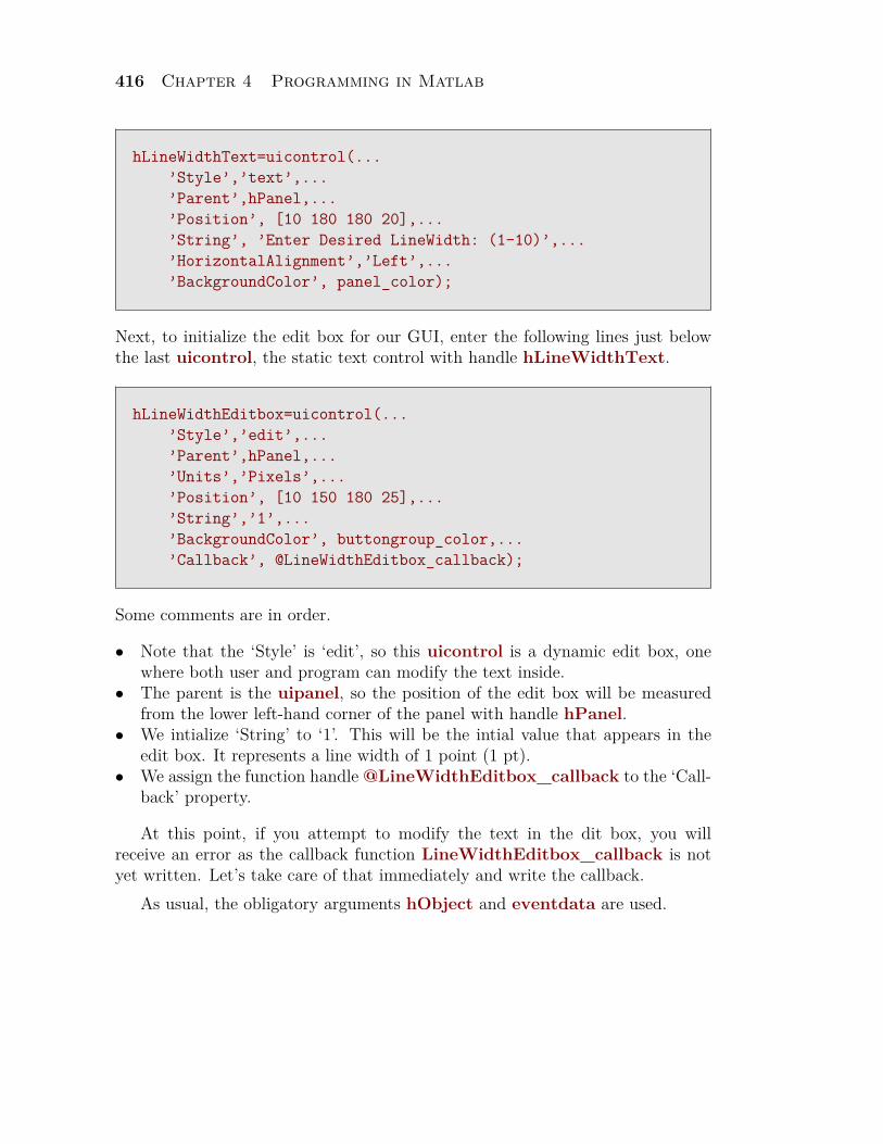
416 Chapter 4 Programming in Matlab
hLineWidthText=uicontrol(...’Style’,’text’,...’Parent’,hPanel,...’Position’, [10 180 180 20],...’String’, ’Enter Desired LineWidth: (1-10)’,...’HorizontalAlignment’,’Left’,...’BackgroundColor’, panel_color);
Next, to initialize the edit box for our GUI, enter the following lines just belowthe last uicontrol, the static text control with handle hLineWidthText.
hLineWidthEditbox=uicontrol(...’Style’,’edit’,...’Parent’,hPanel,...’Units’,’Pixels’,...’Position’, [10 150 180 25],...’String’,’1’,...’BackgroundColor’, buttongroup_color,...’Callback’, @LineWidthEditbox_callback);
Some comments are in order.
• Note that the ‘Style’ is ‘edit’, so this uicontrol is a dynamic edit box, onewhere both user and program can modify the text inside.
• The parent is the uipanel, so the position of the edit box will be measuredfrom the lower left-hand corner of the panel with handle hPanel.
• We intialize ‘String’ to ‘1’. This will be the intial value that appears in theedit box. It represents a line width of 1 point (1 pt).
• We assign the function handle @LineWidthEditbox_callback to the ‘Call-back’ property.
At this point, if you attempt to modify the text in the dit box, you willreceive an error as the callback function LineWidthEditbox_callback is notyet written. Let’s take care of that immediately and write the callback.
As usual, the obligatory arguments hObject and eventdata are used.
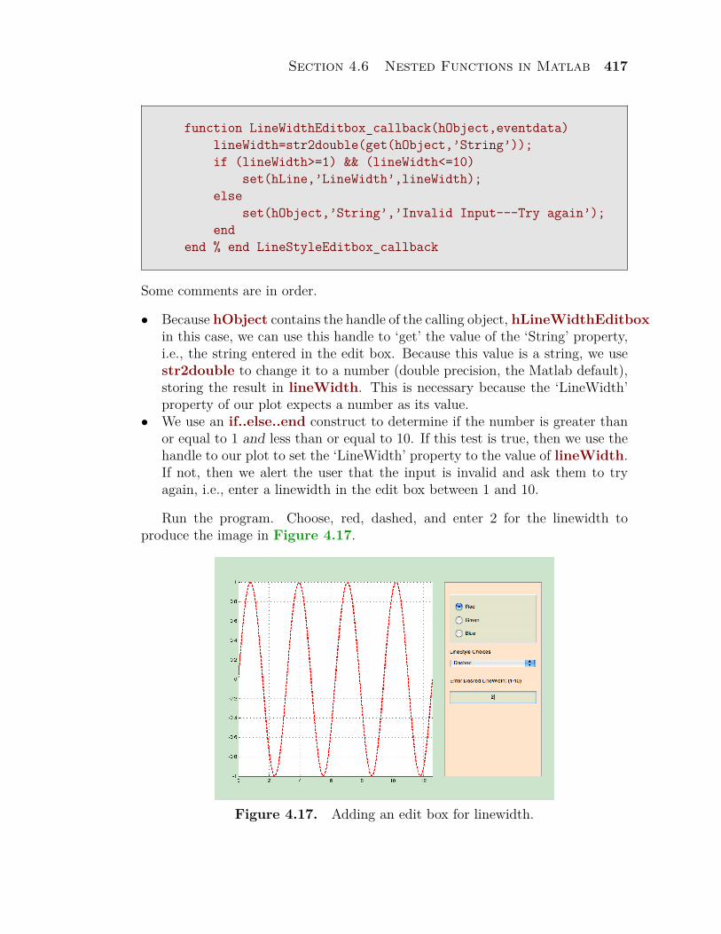
Section 4.6 Nested Functions in Matlab 417
function LineWidthEditbox_callback(hObject,eventdata)lineWidth=str2double(get(hObject,’String’));if (lineWidth>=1) && (lineWidth<=10)
set(hLine,’LineWidth’,lineWidth);else
set(hObject,’String’,’Invalid Input---Try again’);end
end % end LineStyleEditbox_callback
Some comments are in order.
• Because hObject contains the handle of the calling object, hLineWidthEditboxin this case, we can use this handle to ‘get’ the value of the ‘String’ property,i.e., the string entered in the edit box. Because this value is a string, we usestr2double to change it to a number (double precision, the Matlab default),storing the result in lineWidth. This is necessary because the ‘LineWidth’property of our plot expects a number as its value.
• We use an if..else..end construct to determine if the number is greater thanor equal to 1 and less than or equal to 10. If this test is true, then we use thehandle to our plot to set the ‘LineWidth’ property to the value of lineWidth.If not, then we alert the user that the input is invalid and ask them to tryagain, i.e., enter a linewidth in the edit box between 1 and 10.
Run the program. Choose, red, dashed, and enter 2 for the linewidth toproduce the image in Figure 4.17.
Figure 4.17. Adding an edit box for linewidth.
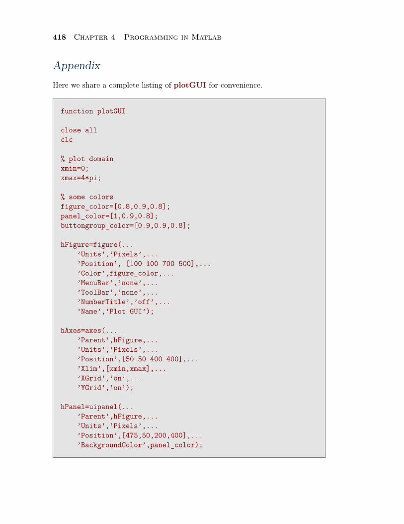
418 Chapter 4 Programming in Matlab
AppendixHere we share a complete listing of plotGUI for convenience.
function plotGUI
close allclc
% plot domainxmin=0;xmax=4*pi;
% some colorsfigure_color=[0.8,0.9,0.8];panel_color=[1,0.9,0.8];buttongroup_color=[0.9,0.9,0.8];
hFigure=figure(...’Units’,’Pixels’,...’Position’, [100 100 700 500],...’Color’,figure_color,...’MenuBar’,’none’,...’ToolBar’,’none’,...’NumberTitle’,’off’,...’Name’,’Plot GUI’);
hAxes=axes(...’Parent’,hFigure,...’Units’,’Pixels’,...’Position’,[50 50 400 400],...’Xlim’,[xmin,xmax],...’XGrid’,’on’,...’YGrid’,’on’);
hPanel=uipanel(...’Parent’,hFigure,...’Units’,’Pixels’,...’Position’,[475,50,200,400],...’BackgroundColor’,panel_color);
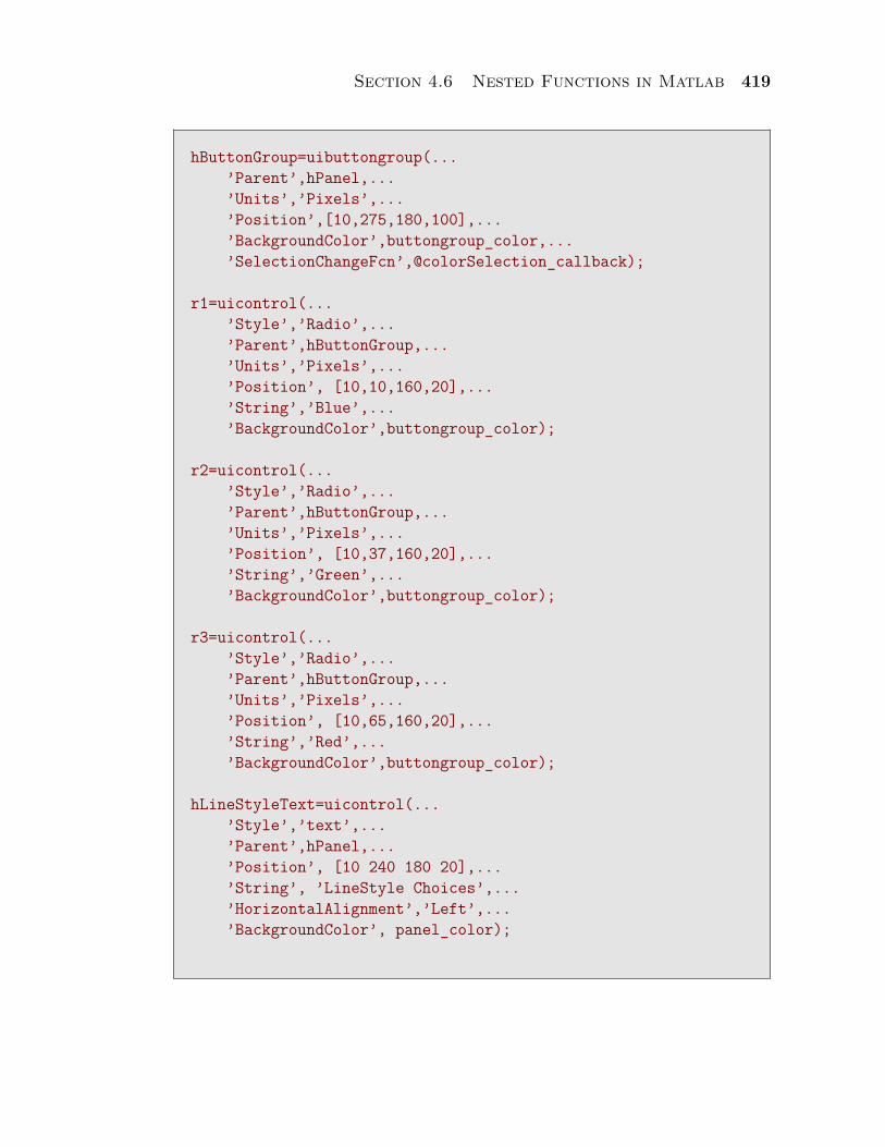
Section 4.6 Nested Functions in Matlab 419
hButtonGroup=uibuttongroup(...’Parent’,hPanel,...’Units’,’Pixels’,...’Position’,[10,275,180,100],...’BackgroundColor’,buttongroup_color,...’SelectionChangeFcn’,@colorSelection_callback);
r1=uicontrol(...’Style’,’Radio’,...’Parent’,hButtonGroup,...’Units’,’Pixels’,...’Position’, [10,10,160,20],...’String’,’Blue’,...’BackgroundColor’,buttongroup_color);
r2=uicontrol(...’Style’,’Radio’,...’Parent’,hButtonGroup,...’Units’,’Pixels’,...’Position’, [10,37,160,20],...’String’,’Green’,...’BackgroundColor’,buttongroup_color);
r3=uicontrol(...’Style’,’Radio’,...’Parent’,hButtonGroup,...’Units’,’Pixels’,...’Position’, [10,65,160,20],...’String’,’Red’,...’BackgroundColor’,buttongroup_color);
hLineStyleText=uicontrol(...’Style’,’text’,...’Parent’,hPanel,...’Position’, [10 240 180 20],...’String’, ’LineStyle Choices’,...’HorizontalAlignment’,’Left’,...’BackgroundColor’, panel_color);
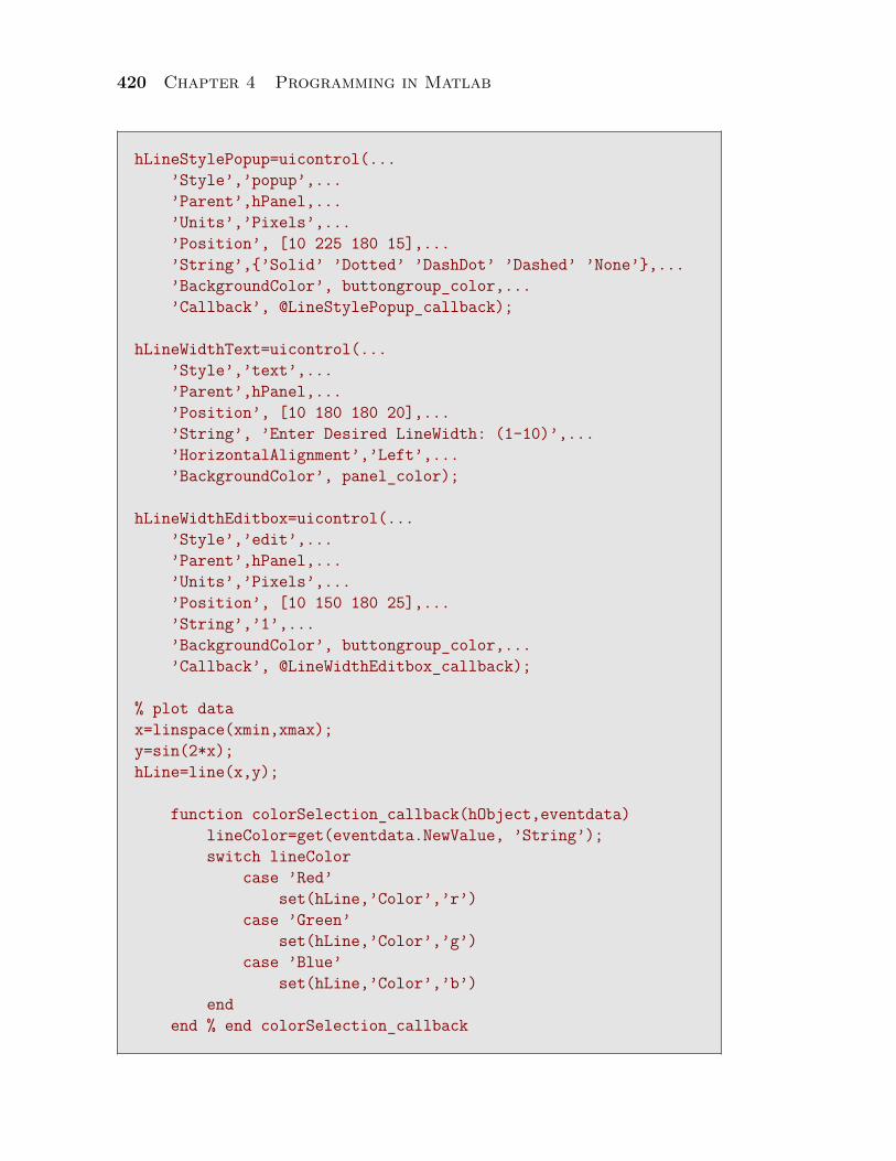
420 Chapter 4 Programming in Matlab
hLineStylePopup=uicontrol(...’Style’,’popup’,...’Parent’,hPanel,...’Units’,’Pixels’,...’Position’, [10 225 180 15],...’String’,{’Solid’ ’Dotted’ ’DashDot’ ’Dashed’ ’None’},...’BackgroundColor’, buttongroup_color,...’Callback’, @LineStylePopup_callback);
hLineWidthText=uicontrol(...’Style’,’text’,...’Parent’,hPanel,...’Position’, [10 180 180 20],...’String’, ’Enter Desired LineWidth: (1-10)’,...’HorizontalAlignment’,’Left’,...’BackgroundColor’, panel_color);
hLineWidthEditbox=uicontrol(...’Style’,’edit’,...’Parent’,hPanel,...’Units’,’Pixels’,...’Position’, [10 150 180 25],...’String’,’1’,...’BackgroundColor’, buttongroup_color,...’Callback’, @LineWidthEditbox_callback);
% plot datax=linspace(xmin,xmax);y=sin(2*x);hLine=line(x,y);
function colorSelection_callback(hObject,eventdata)lineColor=get(eventdata.NewValue, ’String’);switch lineColor
case ’Red’set(hLine,’Color’,’r’)
case ’Green’set(hLine,’Color’,’g’)
case ’Blue’set(hLine,’Color’,’b’)
endend % end colorSelection_callback
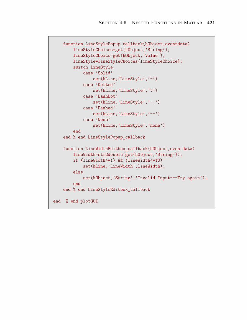
Section 4.6 Nested Functions in Matlab 421
function LineStylePopup_callback(hObject,eventdata)lineStyleChoices=get(hObject,’String’);lineStyleChoice=get(hObject,’Value’);lineStyle=lineStyleChoices{lineStyleChoice};switch lineStyle
case ’Solid’set(hLine,’LineStyle’,’-’)
case ’Dotted’set(hLine,’LineStyle’,’:’)
case ’DashDot’set(hLine,’LineStyle’,’-.’)
case ’Dashed’set(hLine,’LineStyle’,’--’)
case ’None’set(hLine,’LineStyle’,’none’)
endend % end LineStylePopup_callback
function LineWidthEditbox_callback(hObject,eventdata)lineWidth=str2double(get(hObject,’String’));if (lineWidth>=1) && (lineWidth<=10)
set(hLine,’LineWidth’,lineWidth);else
set(hObject,’String’,’Invalid Input---Try again’);end
end % end LineStyleEditbox_callback
end % end plotGUI
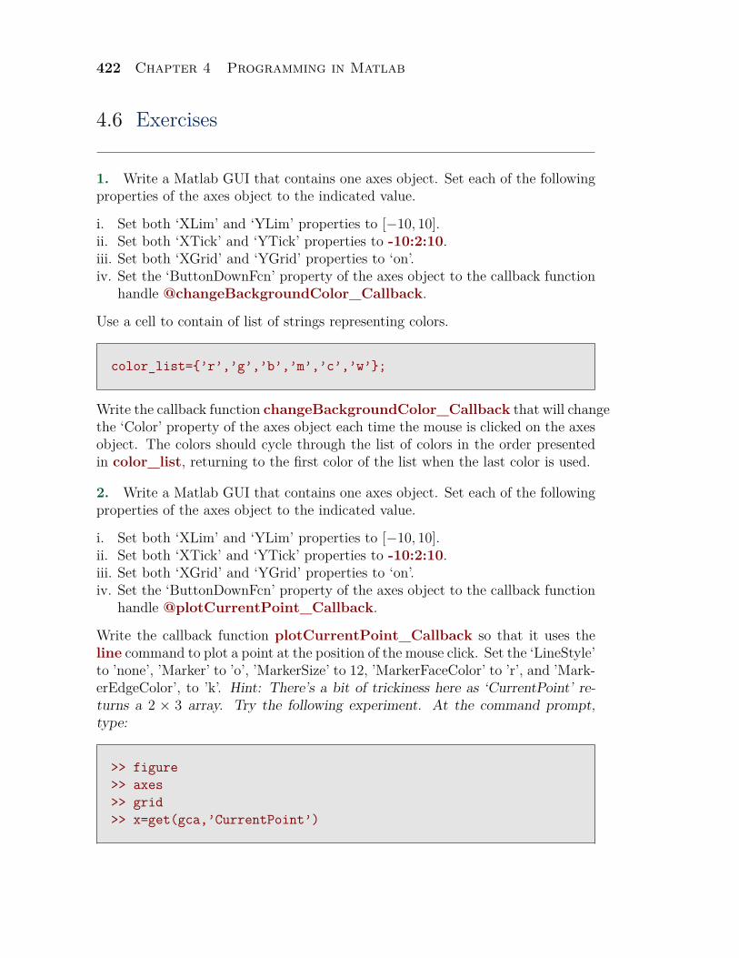
422 Chapter 4 Programming in Matlab
4.6 Exercises
1. Write a Matlab GUI that contains one axes object. Set each of the followingproperties of the axes object to the indicated value.
i. Set both ‘XLim’ and ‘YLim’ properties to [−10, 10].ii. Set both ‘XTick’ and ‘YTick’ properties to -10:2:10.iii. Set both ‘XGrid’ and ‘YGrid’ properties to ‘on’.iv. Set the ‘ButtonDownFcn’ property of the axes object to the callback function
handle @changeBackgroundColor_Callback.
Use a cell to contain of list of strings representing colors.
color_list={’r’,’g’,’b’,’m’,’c’,’w’};
Write the callback function changeBackgroundColor_Callback that will changethe ‘Color’ property of the axes object each time the mouse is clicked on the axesobject. The colors should cycle through the list of colors in the order presentedin color_list, returning to the first color of the list when the last color is used.
2. Write a Matlab GUI that contains one axes object. Set each of the followingproperties of the axes object to the indicated value.
i. Set both ‘XLim’ and ‘YLim’ properties to [−10, 10].ii. Set both ‘XTick’ and ‘YTick’ properties to -10:2:10.iii. Set both ‘XGrid’ and ‘YGrid’ properties to ‘on’.iv. Set the ‘ButtonDownFcn’ property of the axes object to the callback function
handle @plotCurrentPoint_Callback.
Write the callback function plotCurrentPoint_Callback so that it uses theline command to plot a point at the position of the mouse click. Set the ‘LineStyle’to ’none’, ’Marker’ to ’o’, ’MarkerSize’ to 12, ’MarkerFaceColor’ to ’r’, and ’Mark-erEdgeColor’, to ’k’. Hint: There’s a bit of trickiness here as ‘CurrentPoint’ re-turns a 2 × 3 array. Try the following experiment. At the command prompt,type:
>> figure>> axes>> grid>> x=get(gca,’CurrentPoint’)
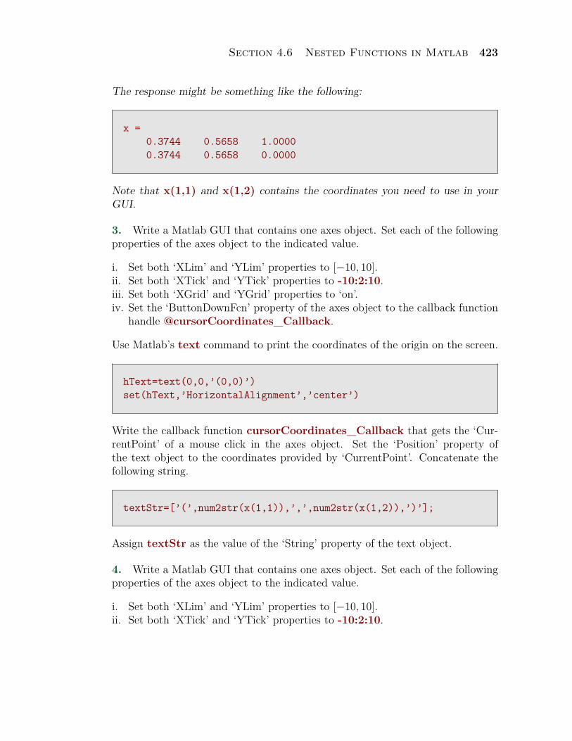
Section 4.6 Nested Functions in Matlab 423
The response might be something like the following:
x =0.3744 0.5658 1.00000.3744 0.5658 0.0000
Note that x(1,1) and x(1,2) contains the coordinates you need to use in yourGUI.
3. Write a Matlab GUI that contains one axes object. Set each of the followingproperties of the axes object to the indicated value.
i. Set both ‘XLim’ and ‘YLim’ properties to [−10, 10].ii. Set both ‘XTick’ and ‘YTick’ properties to -10:2:10.iii. Set both ‘XGrid’ and ‘YGrid’ properties to ‘on’.iv. Set the ‘ButtonDownFcn’ property of the axes object to the callback function
handle @cursorCoordinates_Callback.
Use Matlab’s text command to print the coordinates of the origin on the screen.
hText=text(0,0,’(0,0)’)set(hText,’HorizontalAlignment’,’center’)
Write the callback function cursorCoordinates_Callback that gets the ‘Cur-rentPoint’ of a mouse click in the axes object. Set the ‘Position’ property ofthe text object to the coordinates provided by ‘CurrentPoint’. Concatenate thefollowing string.
textStr=[’(’,num2str(x(1,1)),’,’,num2str(x(1,2)),’)’];
Assign textStr as the value of the ‘String’ property of the text object.
4. Write a Matlab GUI that contains one axes object. Set each of the followingproperties of the axes object to the indicated value.
i. Set both ‘XLim’ and ‘YLim’ properties to [−10, 10].ii. Set both ‘XTick’ and ‘YTick’ properties to -10:2:10.
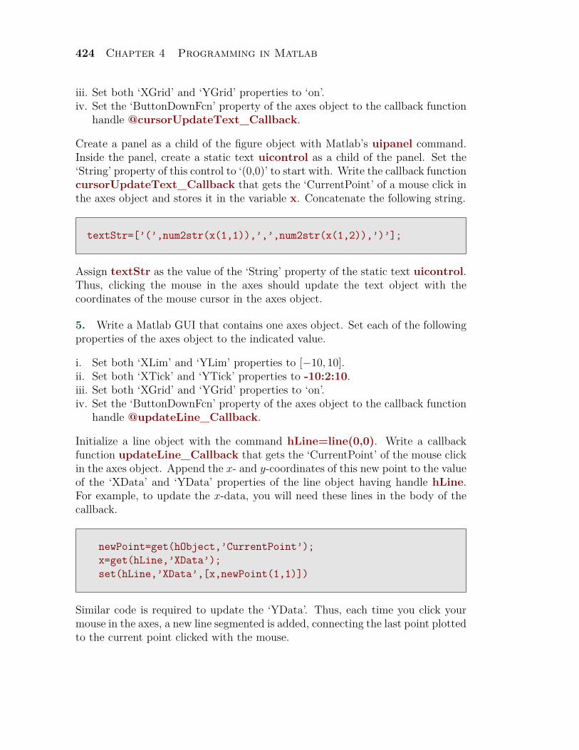
424 Chapter 4 Programming in Matlab
iii. Set both ‘XGrid’ and ‘YGrid’ properties to ‘on’.iv. Set the ‘ButtonDownFcn’ property of the axes object to the callback function
handle @cursorUpdateText_Callback.
Create a panel as a child of the figure object with Matlab’s uipanel command.Inside the panel, create a static text uicontrol as a child of the panel. Set the‘String’ property of this control to ‘(0,0)’ to start with. Write the callback functioncursorUpdateText_Callback that gets the ‘CurrentPoint’ of a mouse click inthe axes object and stores it in the variable x. Concatenate the following string.
textStr=[’(’,num2str(x(1,1)),’,’,num2str(x(1,2)),’)’];
Assign textStr as the value of the ‘String’ property of the static text uicontrol.Thus, clicking the mouse in the axes should update the text object with thecoordinates of the mouse cursor in the axes object.
5. Write a Matlab GUI that contains one axes object. Set each of the followingproperties of the axes object to the indicated value.
i. Set both ‘XLim’ and ‘YLim’ properties to [−10, 10].ii. Set both ‘XTick’ and ‘YTick’ properties to -10:2:10.iii. Set both ‘XGrid’ and ‘YGrid’ properties to ‘on’.iv. Set the ‘ButtonDownFcn’ property of the axes object to the callback function
handle @updateLine_Callback.
Initialize a line object with the command hLine=line(0,0). Write a callbackfunction updateLine_Callback that gets the ‘CurrentPoint’ of the mouse clickin the axes object. Append the x- and y-coordinates of this new point to the valueof the ‘XData’ and ‘YData’ properties of the line object having handle hLine.For example, to update the x-data, you will need these lines in the body of thecallback.
newPoint=get(hObject,’CurrentPoint’);x=get(hLine,’XData’);set(hLine,’XData’,[x,newPoint(1,1)])
Similar code is required to update the ‘YData’. Thus, each time you click yourmouse in the axes, a new line segmented is added, connecting the last point plottedto the current point clicked with the mouse.
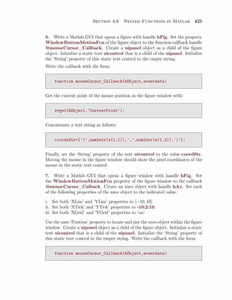
Section 4.6 Nested Functions in Matlab 425
6. Write a Matlab GUI that opens a figure with handle hFig. Set the propertyWindowButtonMotionFcn of the figure object to the function callback handle@mouseCursor_Callback. Create a uipanel object as a child of the figureobject. Initialize a static text uicontrol that is a child of the uipanel. Initializethe ‘String’ property of this static text control to the empty string.Write the callback with the form:
function mouseCursor_Callback(hObject,eventdata)
Get the current point of the mouse position in the figure window with:
x=get(hObject,’CurrentPoint’);
Concatenate a text string as follows:
coordsStr=[’(’,num2str(x(1,1)),’,’,num2str(x(1,2)),’)’];
Finally, set the ‘String’ property of the text uicontrol to the value coordStr.Moving the mouse in the figure window should show the pixel coordinates of themouse in the static text control.
7. Write a Matlab GUI that opens a figure window with handle hFig. Setthe WindowButtonMotionFcn property of the figure window to the callback@mouseCursor_Calback. Create an axes object with handle hAx. Set eachof the following properties of the axes object to the indicated value.
i. Set both ‘XLim’ and ‘YLim’ properties to [−10, 10].ii. Set both ‘XTick’ and ‘YTick’ properties to -10:2:10.iii. Set both ‘XGrid’ and ‘YGrid’ properties to ‘on’.
Use the axes ‘Position’ property to locate and size the axes object within the figurewindow. Create a uipanel object as a child of the figure object. Initialize a statictext uicontrol that is a child of the uipanel. Initialize the ‘String’ property ofthis static text control to the empty string. Write the callback with the form:
function mouseCursor_Callback(hObject,eventdata)
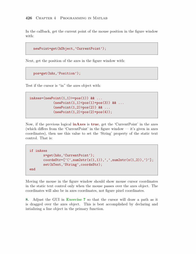
426 Chapter 4 Programming in Matlab
In the callback, get the current point of the mouse position in the figure windowwith:
newPoint=get(hObject,’CurrentPoint’);
Next, get the position of the axes in the figure window with:
pos=get(hAx,’Position’);
Test if the cursor is “in” the axes object with:
inAxes=(newPoint(1,1)>=pos(1)) && ...(newPoint(1,1)<pos(1)+pos(3)) && ...(newPoint(1,2)>pos(2)) && ...(newPoint(1,2)<pos(2)+pos(4));
Now, if the previous logical inAxes is true, get the ‘CurrentPoint’ in the axes(which differs from the ‘CurrentPoint’ in the figure window — it’s given in axescoordinates), then use this value to set the ‘String’ property of the static textcontrol. That is:
if inAxesx=get(hAx,’CurrentPoint’);coordsStr=[’(’,num2str(x(1,1)),’,’,num2str(x(1,2)),’)’];set(hText,’String’,coordsStr);
end
Moving the mouse in the figure window should show mouse cursor coordinatesin the static text control only when the mouse passes over the axes object. Thecoordinates will also be in axes coordinates, not figure pixel coordinates.
8. Adjust the GUI in Exercise 7 so that the cursor will draw a path as itis dragged over the axes object. This is best accomplished by declaring andintializing a line object in the primary function.
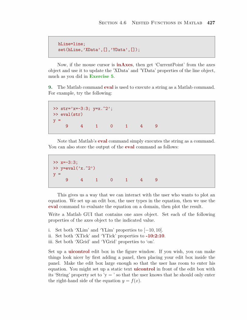
Section 4.6 Nested Functions in Matlab 427
hLine=line;set(hLine,’XData’,[],’YData’,[]);
Now, if the mouse cursor is inAxes, then get ‘CurrentPoint’ from the axesobject and use it to update the ’XData’ and ’YData’ properties of the line object,much as you did in Exercise 5.
9. The Matlab command eval is used to execute a string as a Matlab command.For example, try the following:
>> str=’x=-3:3; y=x.^2’;>> eval(str)y =
9 4 1 0 1 4 9
Note that Matlab’s eval command simply executes the string as a command.You can also store the output of the eval command as follows:
>> x=-3:3;>> y=eval(’x.^2’)y =
9 4 1 0 1 4 9
This gives us a way that we can interact with the user who wants to plot anequation. We set up an edit box, the user types in the equation, then we use theeval command to evaluate the equation on a domain, then plot the result.Write a Matlab GUI that contains one axes object. Set each of the followingproperties of the axes object to the indicated value.
i. Set both ‘XLim’ and ‘YLim’ properties to [−10, 10].ii. Set both ‘XTick’ and ‘YTick’ properties to -10:2:10.iii. Set both ‘XGrid’ and ‘YGrid’ properties to ‘on’.
Set up a uicontrol edit box in the figure window. If you wish, you can makethings look nicer by first adding a panel, then placing your edit box inside thepanel. Make the edit box large enough so that the user has room to enter hisequation. You might set up a static text uicontrol in front of the edit box withits ‘String’ property set to ’y = ’ so that the user knows that he should only enterthe right-hand side of the equation y = f(x).
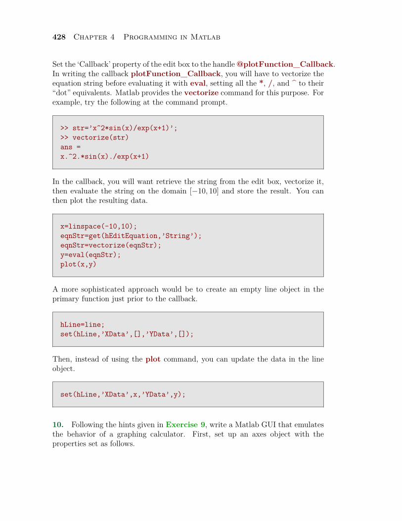
428 Chapter 4 Programming in Matlab
Set the ‘Callback’ property of the edit box to the handle @plotFunction_Callback.In writing the callback plotFunction_Callback, you will have to vectorize theequation string before evaluating it with eval, setting all the *, /, and ^ to their“dot” equivalents. Matlab provides the vectorize command for this purpose. Forexample, try the following at the command prompt.
>> str=’x^2*sin(x)/exp(x+1)’;>> vectorize(str)ans =x.^2.*sin(x)./exp(x+1)
In the callback, you will want retrieve the string from the edit box, vectorize it,then evaluate the string on the domain [−10, 10] and store the result. You canthen plot the resulting data.
x=linspace(-10,10);eqnStr=get(hEditEquation,’String’);eqnStr=vectorize(eqnStr);y=eval(eqnStr);plot(x,y)
A more sophisticated approach would be to create an empty line object in theprimary function just prior to the callback.
hLine=line;set(hLine,’XData’,[],’YData’,[]);
Then, instead of using the plot command, you can update the data in the lineobject.
set(hLine,’XData’,x,’YData’,y);
10. Following the hints given in Exercise 9, write a Matlab GUI that emulatesthe behavior of a graphing calculator. First, set up an axes object with theproperties set as follows.
Section 4.6 Nested Functions in Matlab 429
i. Set both ‘XLim’ and ‘YLim’ properties to [−10, 10].ii. Set both ‘XTick’ and ‘YTick’ properties to -10:2:10.iii. Set both ‘XGrid’ and ‘YGrid’ properties to ‘on’.
Create three panels. One panel will hold an edit box where the user enters hisequation, a second will hold edit boxes for the window parameters xmin, xmax,xscl, ymin, ymax, and yscl. You might also want to create an edit box in this sec-ond panel that contains the number of points to be plotted. Should a graph have a“jagged” appearance, increasing the number in this edit box would smoothen thegraph. A third panel should contain a uicontrol that is a pushbutton. This push-button should have its ‘String’ property set to ‘Graph’ and ‘Callback’ propertyset to the handle @plotFunction_Callback.The design should allow the user to enter his equation, window parameters, andnumber of points. When the user clicks the pushbutton with his mouse, thecallback function plotFunction_Callback will grab the window parameter dataand adjust ‘Xlim’, ‘YLim’, ‘XTick’, and ‘YTick’ of the axes object accordingly.Then the user’s equation should be drawn over the domain [Xmin,Xmax].This problem could potentially be expanded into a semester ending project,adding ‘Zoom’ menu or a ‘Calc’ menu for finding zeros and extrema. This projectis very open-ended with lots of potential for further implementation of ideas andutilities.
430 Chapter 4 Programming in Matlab
4.6 Answers
2. linePlot.m
4. cursorText.m
8. mouseDraw.m


