Embed Size (px)
Citation preview
CDO User’s Guide
Climate Data OperatorsVersion 1.4.7January 2011
Uwe Schulzweida, Luis Kornblueh – MPI for Meteorology
Ralf Quast – Brockmann Consult
Contents
1. Introduction 61.1. Building from sources . . . . . . . . . . . . . . . . . . . . . . . . . . . . . . . . . . . . . . . 6
1.1.1. Compilation . . . . . . . . . . . . . . . . . . . . . . . . . . . . . . . . . . . . . . . . . 71.1.2. Installation . . . . . . . . . . . . . . . . . . . . . . . . . . . . . . . . . . . . . . . . . 7
1.2. Usage . . . . . . . . . . . . . . . . . . . . . . . . . . . . . . . . . . . . . . . . . . . . . . . . 81.2.1. Options . . . . . . . . . . . . . . . . . . . . . . . . . . . . . . . . . . . . . . . . . . . 81.2.2. Operators . . . . . . . . . . . . . . . . . . . . . . . . . . . . . . . . . . . . . . . . . . 81.2.3. Combining operators . . . . . . . . . . . . . . . . . . . . . . . . . . . . . . . . . . . . 91.2.4. Operator parameter . . . . . . . . . . . . . . . . . . . . . . . . . . . . . . . . . . . . 9
1.3. Grid description . . . . . . . . . . . . . . . . . . . . . . . . . . . . . . . . . . . . . . . . . . 91.3.1. Predefined grids . . . . . . . . . . . . . . . . . . . . . . . . . . . . . . . . . . . . . . 101.3.2. Grids from data files . . . . . . . . . . . . . . . . . . . . . . . . . . . . . . . . . . . . 101.3.3. SCRIP grids . . . . . . . . . . . . . . . . . . . . . . . . . . . . . . . . . . . . . . . . 101.3.4. PINGO grids . . . . . . . . . . . . . . . . . . . . . . . . . . . . . . . . . . . . . . . . 111.3.5. CDO grids . . . . . . . . . . . . . . . . . . . . . . . . . . . . . . . . . . . . . . . . . 11
1.4. Z-axis description . . . . . . . . . . . . . . . . . . . . . . . . . . . . . . . . . . . . . . . . . . 121.5. Time axis . . . . . . . . . . . . . . . . . . . . . . . . . . . . . . . . . . . . . . . . . . . . . . 13
1.5.1. Absolute time . . . . . . . . . . . . . . . . . . . . . . . . . . . . . . . . . . . . . . . . 131.5.2. Relative time . . . . . . . . . . . . . . . . . . . . . . . . . . . . . . . . . . . . . . . . 141.5.3. Conversion of the time . . . . . . . . . . . . . . . . . . . . . . . . . . . . . . . . . . . 14
1.6. Parameter table . . . . . . . . . . . . . . . . . . . . . . . . . . . . . . . . . . . . . . . . . . . 141.7. Missing values . . . . . . . . . . . . . . . . . . . . . . . . . . . . . . . . . . . . . . . . . . . . 14
1.7.1. Mean and average . . . . . . . . . . . . . . . . . . . . . . . . . . . . . . . . . . . . . 15
2. Reference manual 162.1. Information . . . . . . . . . . . . . . . . . . . . . . . . . . . . . . . . . . . . . . . . . . . . . 17
2.1.1. INFO - Information and simple statistics . . . . . . . . . . . . . . . . . . . . . . . . 182.1.2. SINFO - Short information . . . . . . . . . . . . . . . . . . . . . . . . . . . . . . . . 192.1.3. DIFF - Compare two datasets field by field . . . . . . . . . . . . . . . . . . . . . . . 202.1.4. NINFO - Print the number of parameters, levels or times . . . . . . . . . . . . . . . 212.1.5. SHOWINFO - Show variables, levels or times . . . . . . . . . . . . . . . . . . . . . . 222.1.6. FILEDES - Dataset description . . . . . . . . . . . . . . . . . . . . . . . . . . . . . . 23
2.2. File operations . . . . . . . . . . . . . . . . . . . . . . . . . . . . . . . . . . . . . . . . . . . 242.2.1. COPY - Copy datasets . . . . . . . . . . . . . . . . . . . . . . . . . . . . . . . . . . . 252.2.2. REPLACE - Replace variables . . . . . . . . . . . . . . . . . . . . . . . . . . . . . . 252.2.3. MERGE - Merge datasets . . . . . . . . . . . . . . . . . . . . . . . . . . . . . . . . . 272.2.4. SPLIT - Split a dataset . . . . . . . . . . . . . . . . . . . . . . . . . . . . . . . . . . 282.2.5. SPLITTIME - Split time steps of a dataset . . . . . . . . . . . . . . . . . . . . . . . 292.2.6. SPLITSEL - Split selected time steps . . . . . . . . . . . . . . . . . . . . . . . . . . 30
2.3. Selection . . . . . . . . . . . . . . . . . . . . . . . . . . . . . . . . . . . . . . . . . . . . . . . 312.3.1. SELVAR - Select fields . . . . . . . . . . . . . . . . . . . . . . . . . . . . . . . . . . . 322.3.2. SELTIME - Select time steps . . . . . . . . . . . . . . . . . . . . . . . . . . . . . . . 342.3.3. SELBOX - Select a box of a field . . . . . . . . . . . . . . . . . . . . . . . . . . . . . 36
2.4. Conditional selection . . . . . . . . . . . . . . . . . . . . . . . . . . . . . . . . . . . . . . . . 372.4.1. COND - Conditional select one field . . . . . . . . . . . . . . . . . . . . . . . . . . . 382.4.2. COND2 - Conditional select two fields . . . . . . . . . . . . . . . . . . . . . . . . . . 382.4.3. CONDC - Conditional select a constant . . . . . . . . . . . . . . . . . . . . . . . . . 40
2.5. Comparison . . . . . . . . . . . . . . . . . . . . . . . . . . . . . . . . . . . . . . . . . . . . . 412.5.1. COMP - Comparison of two fields . . . . . . . . . . . . . . . . . . . . . . . . . . . . 42
2
Contents Contents
2.5.2. COMPC - Comparison of a field with a constant . . . . . . . . . . . . . . . . . . . . 432.6. Modification . . . . . . . . . . . . . . . . . . . . . . . . . . . . . . . . . . . . . . . . . . . . . 44
2.6.1. SET - Set field info . . . . . . . . . . . . . . . . . . . . . . . . . . . . . . . . . . . . . 452.6.2. SETTIME - Set time . . . . . . . . . . . . . . . . . . . . . . . . . . . . . . . . . . . . 462.6.3. CHANGE - Change field header . . . . . . . . . . . . . . . . . . . . . . . . . . . . . 482.6.4. SETGRID - Set grid type . . . . . . . . . . . . . . . . . . . . . . . . . . . . . . . . . 492.6.5. SETZAXIS - Set z-axis type . . . . . . . . . . . . . . . . . . . . . . . . . . . . . . . . 492.6.6. SETGATT - Set global attribute . . . . . . . . . . . . . . . . . . . . . . . . . . . . . 502.6.7. INVERT - Invert latitudes . . . . . . . . . . . . . . . . . . . . . . . . . . . . . . . . . 512.6.8. INVERTLEV - Invert levels . . . . . . . . . . . . . . . . . . . . . . . . . . . . . . . . 512.6.9. MASKREGION - Mask regions . . . . . . . . . . . . . . . . . . . . . . . . . . . . . . 522.6.10. MASKBOX - Mask a box . . . . . . . . . . . . . . . . . . . . . . . . . . . . . . . . . 532.6.11. SETBOX - Set a box to constant . . . . . . . . . . . . . . . . . . . . . . . . . . . . . 542.6.12. ENLARGE - Enlarge fields . . . . . . . . . . . . . . . . . . . . . . . . . . . . . . . . 552.6.13. SETMISS - Set missing value . . . . . . . . . . . . . . . . . . . . . . . . . . . . . . . 56
2.7. Arithmetic . . . . . . . . . . . . . . . . . . . . . . . . . . . . . . . . . . . . . . . . . . . . . . 582.7.1. EXPR - Evaluate expressions . . . . . . . . . . . . . . . . . . . . . . . . . . . . . . . 592.7.2. MATH - Mathematical functions . . . . . . . . . . . . . . . . . . . . . . . . . . . . . 612.7.3. ARITHC - Arithmetic with a constant . . . . . . . . . . . . . . . . . . . . . . . . . . 622.7.4. ARITH - Arithmetic on two datasets . . . . . . . . . . . . . . . . . . . . . . . . . . . 632.7.5. MONARITH - Monthly arithmetic . . . . . . . . . . . . . . . . . . . . . . . . . . . . 642.7.6. YMONARITH - Multi-year monthly arithmetic . . . . . . . . . . . . . . . . . . . . . 652.7.7. YDAYARITH - Multi-year daily arithmetic . . . . . . . . . . . . . . . . . . . . . . . 662.7.8. ARITHDAYS - Arithmetic with days . . . . . . . . . . . . . . . . . . . . . . . . . . 67
2.8. Statistical values . . . . . . . . . . . . . . . . . . . . . . . . . . . . . . . . . . . . . . . . . . 682.8.1. CONSECSTAT - Consecute timestep periods . . . . . . . . . . . . . . . . . . . . . . 732.8.2. ENSSTAT - Statistical values over an ensemble . . . . . . . . . . . . . . . . . . . . . 742.8.3. ENSSTAT2 - Statistical values over an ensemble . . . . . . . . . . . . . . . . . . . . 762.8.4. FLDSTAT - Statistical values over a field . . . . . . . . . . . . . . . . . . . . . . . . 782.8.5. ZONSTAT - Zonal statistical values . . . . . . . . . . . . . . . . . . . . . . . . . . . 802.8.6. MERSTAT - Meridional statistical values . . . . . . . . . . . . . . . . . . . . . . . . 822.8.7. GRIDBOXSTAT - Statistical values over grid boxes . . . . . . . . . . . . . . . . . . 842.8.8. VERTSTAT - Vertical statistical values . . . . . . . . . . . . . . . . . . . . . . . . . 852.8.9. TIMSELSTAT - Time range statistical values . . . . . . . . . . . . . . . . . . . . . . 862.8.10. TIMSELPCTL - Time range percentile values . . . . . . . . . . . . . . . . . . . . . . 872.8.11. RUNSTAT - Running statistical values . . . . . . . . . . . . . . . . . . . . . . . . . . 882.8.12. RUNPCTL - Running percentile values . . . . . . . . . . . . . . . . . . . . . . . . . 892.8.13. TIMSTAT - Statistical values over all time steps . . . . . . . . . . . . . . . . . . . . 902.8.14. TIMPCTL - Percentile values over all time steps . . . . . . . . . . . . . . . . . . . . 912.8.15. HOURSTAT - Hourly statistical values . . . . . . . . . . . . . . . . . . . . . . . . . 922.8.16. HOURPCTL - Hourly percentile values . . . . . . . . . . . . . . . . . . . . . . . . . 932.8.17. DAYSTAT - Daily statistical values . . . . . . . . . . . . . . . . . . . . . . . . . . . 942.8.18. DAYPCTL - Daily percentile values . . . . . . . . . . . . . . . . . . . . . . . . . . . 952.8.19. MONSTAT - Monthly statistical values . . . . . . . . . . . . . . . . . . . . . . . . . 962.8.20. MONPCTL - Monthly percentile values . . . . . . . . . . . . . . . . . . . . . . . . . 972.8.21. YEARSTAT - Yearly statistical values . . . . . . . . . . . . . . . . . . . . . . . . . . 982.8.22. YEARPCTL - Yearly percentile values . . . . . . . . . . . . . . . . . . . . . . . . . . 992.8.23. SEASSTAT - Seasonal statistical values . . . . . . . . . . . . . . . . . . . . . . . . . 1002.8.24. SEASPCTL - Seasonal percentile values . . . . . . . . . . . . . . . . . . . . . . . . . 1012.8.25. YHOURSTAT - Multi-year hourly statistical values . . . . . . . . . . . . . . . . . . 1022.8.26. YDAYSTAT - Multi-year daily statistical values . . . . . . . . . . . . . . . . . . . . 1032.8.27. YDAYPCTL - Multi-year daily percentile values . . . . . . . . . . . . . . . . . . . . 1042.8.28. YMONSTAT - Multi-year monthly statistical values . . . . . . . . . . . . . . . . . . 1052.8.29. YMONPCTL - Multi-year monthly percentile values . . . . . . . . . . . . . . . . . . 1062.8.30. YSEASSTAT - Multi-year seasonal statistical values . . . . . . . . . . . . . . . . . . 1072.8.31. YSEASPCTL - Multi-year seasonal percentile values . . . . . . . . . . . . . . . . . . 1082.8.32. YDRUNSTAT - Multi-year daily running statistical values . . . . . . . . . . . . . . . 1092.8.33. YDRUNPCTL - Multi-year daily running percentile values . . . . . . . . . . . . . . 111
3
Contents Contents
2.9. Correlation . . . . . . . . . . . . . . . . . . . . . . . . . . . . . . . . . . . . . . . . . . . . . 1122.9.1. FLDCOR - Correlation of grid space . . . . . . . . . . . . . . . . . . . . . . . . . . . 1132.9.2. TIMCOR - Correlation over time . . . . . . . . . . . . . . . . . . . . . . . . . . . . . 113
2.10. Regression . . . . . . . . . . . . . . . . . . . . . . . . . . . . . . . . . . . . . . . . . . . . . . 1142.10.1. REGRES - Regression . . . . . . . . . . . . . . . . . . . . . . . . . . . . . . . . . . . 1152.10.2. DETREND - Detrend time series . . . . . . . . . . . . . . . . . . . . . . . . . . . . . 1152.10.3. TREND - Trend of time series . . . . . . . . . . . . . . . . . . . . . . . . . . . . . . 1162.10.4. SUBTREND - Subtract a trend . . . . . . . . . . . . . . . . . . . . . . . . . . . . . . 116
2.11. EOFs . . . . . . . . . . . . . . . . . . . . . . . . . . . . . . . . . . . . . . . . . . . . . . . . 1172.11.1. EOFS - Empirical Orthogonal Functions . . . . . . . . . . . . . . . . . . . . . . . . . 1182.11.2. EOFCOEFF - Principal coefficients of EOFs . . . . . . . . . . . . . . . . . . . . . . 120
2.12. Interpolation . . . . . . . . . . . . . . . . . . . . . . . . . . . . . . . . . . . . . . . . . . . . 1212.12.1. REMAPGRID - SCRIP grid interpolation . . . . . . . . . . . . . . . . . . . . . . . . 1222.12.2. GENWEIGHTS - Generate SCRIP grid interpolation weights . . . . . . . . . . . . . 1242.12.3. REMAP - SCRIP grid remapping . . . . . . . . . . . . . . . . . . . . . . . . . . . . 1262.12.4. REMAPETA - Remap vertical hybrid level . . . . . . . . . . . . . . . . . . . . . . . 1272.12.5. INTVERT - Vertical interpolation . . . . . . . . . . . . . . . . . . . . . . . . . . . . 1292.12.6. INTLEVEL - Linear level interpolation . . . . . . . . . . . . . . . . . . . . . . . . . 1302.12.7. INTTIME - Time interpolation . . . . . . . . . . . . . . . . . . . . . . . . . . . . . . 1312.12.8. INTYEAR - Year interpolation . . . . . . . . . . . . . . . . . . . . . . . . . . . . . . 132
2.13. Transformation . . . . . . . . . . . . . . . . . . . . . . . . . . . . . . . . . . . . . . . . . . . 1332.13.1. SPECTRAL - Spectral transformation . . . . . . . . . . . . . . . . . . . . . . . . . . 1342.13.2. WIND - Wind transformation . . . . . . . . . . . . . . . . . . . . . . . . . . . . . . . 136
2.14. Import/Export . . . . . . . . . . . . . . . . . . . . . . . . . . . . . . . . . . . . . . . . . . . 1372.14.1. IMPORTBINARY - Import binary data sets . . . . . . . . . . . . . . . . . . . . . . 1382.14.2. IMPORTCMSAF - Import CM-SAF HDF5 files . . . . . . . . . . . . . . . . . . . . 1392.14.3. IMPORTAMSR - Import AMSR binary files . . . . . . . . . . . . . . . . . . . . . . 1402.14.4. INPUT - Formatted input . . . . . . . . . . . . . . . . . . . . . . . . . . . . . . . . . 1412.14.5. OUTPUT - Formatted output . . . . . . . . . . . . . . . . . . . . . . . . . . . . . . 142
2.15. Miscellaneous . . . . . . . . . . . . . . . . . . . . . . . . . . . . . . . . . . . . . . . . . . . . 1432.15.1. GRADSDES - GrADS data descriptor file . . . . . . . . . . . . . . . . . . . . . . . . 1442.15.2. FILTER - Time series filtering . . . . . . . . . . . . . . . . . . . . . . . . . . . . . . 1452.15.3. GRIDCELL - Grid cell quantities . . . . . . . . . . . . . . . . . . . . . . . . . . . . . 1462.15.4. SMOOTH9 - 9 point smoothing . . . . . . . . . . . . . . . . . . . . . . . . . . . . . . 1472.15.5. REPLACEVALUES - Replace variable values . . . . . . . . . . . . . . . . . . . . . . 1472.15.6. TIMSORT - Timsort . . . . . . . . . . . . . . . . . . . . . . . . . . . . . . . . . . . . 1482.15.7. VARGEN - Generate a field . . . . . . . . . . . . . . . . . . . . . . . . . . . . . . . . 1482.15.8. ROTUV - Rotation . . . . . . . . . . . . . . . . . . . . . . . . . . . . . . . . . . . . 1492.15.9. MASTRFU - Mass stream function . . . . . . . . . . . . . . . . . . . . . . . . . . . . 1492.15.10.HISTOGRAM - Histogram . . . . . . . . . . . . . . . . . . . . . . . . . . . . . . . . 1502.15.11.SETHALO - Set the left and right bounds of a field . . . . . . . . . . . . . . . . . . 1502.15.12.WCT - Windchill temperature . . . . . . . . . . . . . . . . . . . . . . . . . . . . . . 1512.15.13.FDNS - Frost days where no snow index per time period . . . . . . . . . . . . . . . . 1512.15.14.STRWIN - Strong wind days index per time period . . . . . . . . . . . . . . . . . . . 1512.15.15.STRBRE - Strong breeze days index per time period . . . . . . . . . . . . . . . . . . 1522.15.16.STRGAL - Strong gale days index per time period . . . . . . . . . . . . . . . . . . . 1522.15.17.HURR - Hurricane days index per time period . . . . . . . . . . . . . . . . . . . . . 152
2.16. Climate indices . . . . . . . . . . . . . . . . . . . . . . . . . . . . . . . . . . . . . . . . . . . 1532.16.1. ECACDD - Consecutive dry days index per time period . . . . . . . . . . . . . . . . 1552.16.2. ECACFD - Consecutive frost days index per time period . . . . . . . . . . . . . . . 1552.16.3. ECACSU - Consecutive summer days index per time period . . . . . . . . . . . . . . 1562.16.4. ECACWD - Consecutive wet days index per time period . . . . . . . . . . . . . . . . 1562.16.5. ECACWDI - Cold wave duration index wrt mean of reference period . . . . . . . . . 1572.16.6. ECACWFI - Cold-spell days index wrt 10th percentile of reference period . . . . . . 1572.16.7. ECAETR - Intra-period extreme temperature range . . . . . . . . . . . . . . . . . . 1592.16.8. ECAFD - Frost days index per time period . . . . . . . . . . . . . . . . . . . . . . . 1592.16.9. ECAGSL - Thermal Growing season length index . . . . . . . . . . . . . . . . . . . . 1602.16.10.ECAHD - Heating degree days per time period . . . . . . . . . . . . . . . . . . . . . 161
4
Contents Contents
2.16.11.ECAHWDI - Heat wave duration index wrt mean of reference period . . . . . . . . . 1612.16.12.ECAHWFI - Warm spell days index wrt 90th percentile of reference period . . . . . 1622.16.13.ECAID - Ice days index per time period . . . . . . . . . . . . . . . . . . . . . . . . . 1622.16.14.ECAPD - Precipitation days index per time period . . . . . . . . . . . . . . . . . . . 1632.16.15.ECAR75P - Moderate wet days wrt 75th percentile of reference period . . . . . . . . 1642.16.16.ECAR75PTOT - Precipitation percent due to R75p days . . . . . . . . . . . . . . . 1642.16.17.ECAR90P - Wet days wrt 90th percentile of reference period . . . . . . . . . . . . . 1652.16.18.ECAR90PTOT - Precipitation percent due to R90p days . . . . . . . . . . . . . . . 1652.16.19.ECAR95P - Very wet days wrt 95th percentile of reference period . . . . . . . . . . 1662.16.20.ECAR95PTOT - Precipitation percent due to R95p days . . . . . . . . . . . . . . . 1662.16.21.ECAR99P - Extremely wet days wrt 99th percentile of reference period . . . . . . . 1672.16.22.ECAR99PTOT - Precipitation percent due to R99p days . . . . . . . . . . . . . . . 1672.16.23.ECARR1 - Wet days index per time period . . . . . . . . . . . . . . . . . . . . . . . 1682.16.24.ECARX1DAY - Highest one day precipitation amount per time period . . . . . . . . 1682.16.25.ECARX5DAY - Highest five-day precipitation amount per time period . . . . . . . . 1692.16.26.ECASDII - Simple daily intensity index per time period . . . . . . . . . . . . . . . . 1692.16.27.ECASU - Summer days index per time period . . . . . . . . . . . . . . . . . . . . . . 1702.16.28.ECATG10P - Cold days percent wrt 10th percentile of reference period . . . . . . . 1712.16.29.ECATG90P - Warm days percent wrt 90th percentile of reference period . . . . . . 1712.16.30.ECATN10P - Cold nights percent wrt 10th percentile of reference period . . . . . . 1722.16.31.ECATN90P - Warm nights percent wrt 90th percentile of reference period . . . . . . 1722.16.32.ECATR - Tropical nights index per time period . . . . . . . . . . . . . . . . . . . . . 1732.16.33.ECATX10P - Very cold days percent wrt 10th percentile of reference period . . . . . 1732.16.34.ECATX90P - Very warm days percent wrt 90th percentile of reference period . . . . 174
A. Grid description examples 176A.1. Example of a curvilinear grid description . . . . . . . . . . . . . . . . . . . . . . . . . . . . . 176A.2. Example description for unstructured grid cells . . . . . . . . . . . . . . . . . . . . . . . . . 177
Operator index 178
5
1. Introduction
The Climate Data Operators (CDO) software are a collection of many operators for standard processingof climate and forecast model output. The operators include simple statistical and arithmetic functions,data selection and subsampling tools, and spatial interpolation. CDO was developed to have the same setof processing functions for GRIB [GRIB] and netCDF [netCDF] datasets in one package.
The Climate Data Interface [CDI] is used for the fast and file format independent access to GRIB andnetCDF datasets. The local data formats SERVICE, EXTRA and IEG are also supported.
There are some limitations for GRIB and netCDF datasets. A GRIB dataset has to be consistent, similarto netCDF. That means all time steps needs to have the same variables, and within a time step eachvariable may occur only once. NetCDF datasets are only supported for the classic data model and arraysup to 4 dimensions. These dimensions should only be used by the horizontal and vertical grid and thetime. The netCDF attributes should follow the GDT, COARDS or CF Conventions.
The user interface and some operators are similar to the PINGO [PINGO] package. There are also someoperators with the same name as in PINGO but with a different meaning. Appendix A gives an overviewof those operators.
The main CDO features are:
� More than 400 operators available
� Modular design and easily extendable with new operators
� Very simple UNIX command line interface
� A dataset can be processed by several operators, without storing the interim results in files
� Most operators handle datasets with missing values
� Fast processing of large datasets
� Support of many different grid types
� Tested on many UNIX/Linux systems, Cygwin, and MacOS-X
1.1. Building from sources
This section describes how to build CDO from the sources on a UNIX system. CDO uses the GNU configureand build system for compilation. The only requirement is a working ANSI C99 compiler.
First go to the download page (http://code.zmaw.de/projects/cdo) to get the latest distribution, ifyou do not have it yet.
To take full advantage of CDO features the following additional libraries should be installed:
� Unidata netCDF library (http://www.unidata.ucar.edu/packages/netcdf) version 3 or higher.This is needed to process netCDF [netCDF] files with CDO.
� HDF5 szip library (http://www.hdfgroup.org/doc resource/SZIP) version 2.1 or higher.This is needed to process szip compressed GRIB [GRIB] files with CDO.
� HDF5 library (http://www.hdfgroup.org/HDF5) version 1.6 or higher.This is needed to import CM-SAF [CM-SAF] HDF5 files with the CDO operator import cmsaf.
� PROJ.4 library (http://trac.osgeo.org/proj) version 4.6 or higher.This is needed to convert Sinusoidal and Lambert Azimuthal Equal Area coordinates to geographiccoordinates, for e.g. remapping.
6
Introduction Building from sources
1.1.1. Compilation
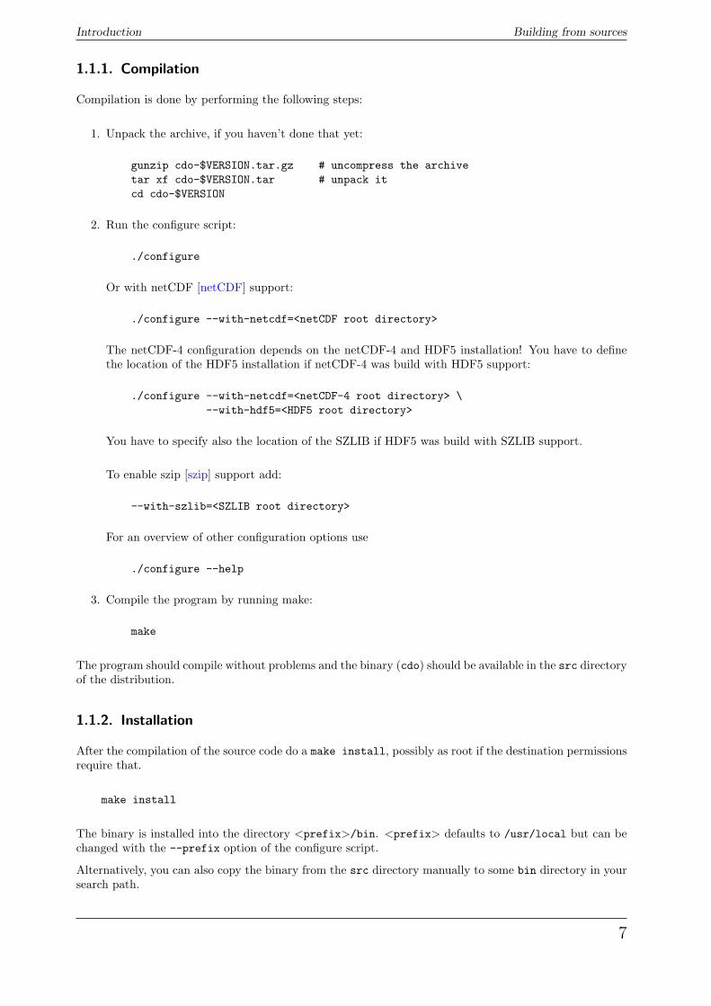
Compilation is done by performing the following steps:
1. Unpack the archive, if you haven’t done that yet:
gunzip cdo-$VERSION.tar.gz # uncompress the archivetar xf cdo-$VERSION.tar # unpack itcd cdo-$VERSION
2. Run the configure script:
./configure
Or with netCDF [netCDF] support:
./configure --with-netcdf=<netCDF root directory>
The netCDF-4 configuration depends on the netCDF-4 and HDF5 installation! You have to definethe location of the HDF5 installation if netCDF-4 was build with HDF5 support:
./configure --with-netcdf=<netCDF-4 root directory> \--with-hdf5=<HDF5 root directory>
You have to specify also the location of the SZLIB if HDF5 was build with SZLIB support.
To enable szip [szip] support add:
--with-szlib=<SZLIB root directory>
For an overview of other configuration options use
./configure --help
3. Compile the program by running make:
make
The program should compile without problems and the binary (cdo) should be available in the src directoryof the distribution.
1.1.2. Installation
After the compilation of the source code do a make install, possibly as root if the destination permissionsrequire that.
make install
The binary is installed into the directory <prefix>/bin. <prefix> defaults to /usr/local but can bechanged with the --prefix option of the configure script.
Alternatively, you can also copy the binary from the src directory manually to some bin directory in yoursearch path.
7
Usage Introduction
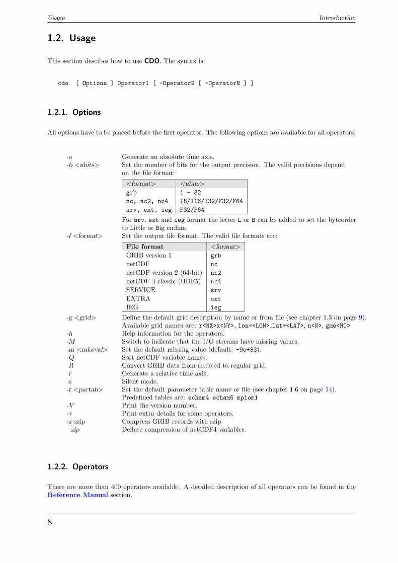
1.2. Usage
This section descibes how to use CDO. The syntax is:
cdo [ Options ] Operator1 [ -Operator2 [ -OperatorN ] ]
1.2.1. Options
All options have to be placed before the first operator. The following options are available for all operators:
-a Generate an absolute time axis.-b <nbits> Set the number of bits for the output precision. The valid precisions depend
on the file format:
<format> <nbits>
grb 1 - 32
nc, nc2, nc4 I8/I16/I32/F32/F64
srv, ext, ieg F32/F64
For srv, ext and ieg format the letter L or B can be added to set the byteorderto Little or Big endian.
-f <format> Set the output file format. The valid file formats are:
File format <format>
GRIB version 1 grb
netCDF nc
netCDF version 2 (64-bit) nc2
netCDF-4 classic (HDF5) nc4
SERVICE srv
EXTRA ext
IEG ieg
-g <grid> Define the default grid description by name or from file (see chapter 1.3 on page 9).Available grid names are: r<NX>x<NY>, lon=<LON> lat=<LAT>, n<N>, gme<NI>
-h Help information for the operators.-M Switch to indicate that the I/O streams have missing values.-m <missval> Set the default missing value (default: -9e+33).-Q Sort netCDF variable names.-R Convert GRIB data from reduced to regular grid.-r Generate a relative time axis.-s Silent mode.-t <partab> Set the default parameter table name or file (see chapter 1.6 on page 14).
Predefined tables are: echam4 echam5 mpiom1-V Print the version number.-v Print extra details for some operators.-z szip Compress GRIB records with szip.
zip Deflate compression of netCDF4 variables.
1.2.2. Operators
There are more than 400 operators available. A detailed description of all operators can be found in theReference Manual section.
8
Introduction Grid description
1.2.3. Combining operators
All operators with a fixed number of input streams and one output stream can pipe the result directlyto an other operator. The operator must begin with ”–”, in order to combine it with others. This canimprove the performance by:
� reducing unnecessary disk I/O
� parallel processing
Use
cdo sub -dayavg ifile2 -timavg ifile1 ofile
instead of
cdo timavg ifile1 tmp1cdo dayavg ifile2 tmp2cdo sub tmp2 tmp1 ofilerm tmp1 tmp2
Combining of operators is implemented over POSIX Threads (pthread). Therefore this CDO feature is notavailable on operating systems without POSIX Threads support.
1.2.4. Operator parameter
Some operators need one or more parameter.
� STRINGUnquoted characters without blanks and tabs. The following command select the variables with thenames pressure and tsurf:
cdo selvar,pressure,tsurf ifile ofile
� FLOATFloating point number in any representation. The following command sets the range between 0 and273.15 of all fields to missing value:
cdo setrtomiss,0,273.15 ifile ofile
� INTEGERA list of integers can be specified by first/last[/inc]. To select the days 5, 6, 7, 8 and 9 use:
cdo selday,5/9 ifile ofile
This is the same as:
cdo selday,5,6,7,8,9 ifile ofile
1.3. Grid description
In the following situations it is necessary to give a description of a horizontal grid:
� Changing the grid description (operator: setgrid)
� Horizontal interpolation (operator: remapXXX and genXXX)
� Generating of variables (operator: const, random)
As now described, there are several possibilities to define a horizontal grid. Predefined grids are availablefor global regular, gaussian or icosahedral-hexagonal GME grids.
9
Grid description Introduction
1.3.1. Predefined grids
The following pre-defined grid names are available: r<NX>x<NY>, lon=<LON> lat=<LAT>, n<N> and gme<NI>
Global regular grid: r<NX>x<NY>
r<NX>x<NY> defines a global regular lon/lat grid. The number of the longitudes <NX> and the latitudes<NY> can be selected at will. The longitudes start at 0◦ with an increment of (360/<NX>)◦. The latitudesgo from south to north with an increment of (180/<NY>)◦.
One grid point: lon=<LON> lat=<LAT>
lon=<LON> lat=<LAT> defines a lon/lat grid with only one grid point.
Global Gaussian grid: n<N>
n<N> defines a global Gaussian grid. N specifies the number of latitudes lines between the Pole and theEquator. The longitudes start at 0◦ with an increment of (360/nlon)◦. The gaussian latitudes go fromnorth to south.
Global icosahedral-hexagonal GME grid: gme<NI>
gme<NI> defines a global icosahedral-hexagonal GME grid. NI specifies the number of intervals on a maintriangle side.
1.3.2. Grids from data files
You can use the grid description from an other datafile. The format of the datafile and the grid of thedata field must be supported by this program. Use the operator ’sinfo’ to get short informations aboutyour variables and the grids. If there are more then one grid in the datafile the grid description of the firstvariable will be used.
1.3.3. SCRIP grids
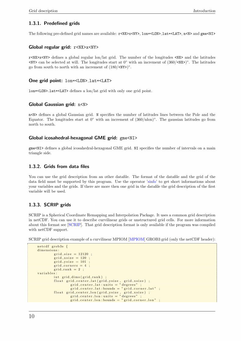
SCRIP is a Spherical Coordinate Remapping and Interpolation Package. It uses a common grid descriptionin netCDF. You can use it to describe curvilinear grids or unstructured grid cells. For more informationabout this format see [SCRIP]. That grid description format is only available if the program was compiledwith netCDF support.
SCRIP grid description example of a curvilinear MPIOM [MPIOM] GROB3 grid (only the netCDF header):
netcd f grob3s {dimensions :
g r i d s i z e = 12120 ;g r i d x s i z e = 120 ;g r i d y s i z e = 101 ;g r i d c o r n e r s = 4 ;g r id rank = 2 ;
v a r i a b l e s :i n t gr id d ims ( g r id rank ) ;f l o a t g r i d c e n t e r l a t ( g r i d y s i z e , g r i d x s i z e ) ;
g r i d c e n t e r l a t : un i t s = ” degree s ” ;g r i d c e n t e r l a t : bounds = ” g r i d c o r n e r l a t ” ;
f l o a t g r i d c e n t e r l o n ( g r i d y s i z e , g r i d x s i z e ) ;g r i d c e n t e r l o n : un i t s = ” degree s ” ;g r i d c e n t e r l o n : bounds = ” g r i d c o r n e r l o n ” ;
10
Introduction Grid description
i n t gr id imask ( g r i d y s i z e , g r i d x s i z e ) ;g r id imask : un i t s = ” u n i t l e s s ” ;g r id imask : coo rd ina t e s = ” g r i d c e n t e r l o n g r i d c e n t e r l a t ” ;
f l o a t g r i d c o r n e r l a t ( g r i d y s i z e , g r i d x s i z e , g r i d c o r n e r s ) ;g r i d c o r n e r l a t : un i t s = ” degree s ” ;
f l o a t g r i d c o r n e r l o n ( g r i d y s i z e , g r i d x s i z e , g r i d c o r n e r s ) ;g r i d c o r n e r l o n : un i t s = ” degree s ” ;
// g l oba l a t t r i b u t e s :: t i t l e = ” grob3s ” ;
}
1.3.4. PINGO grids
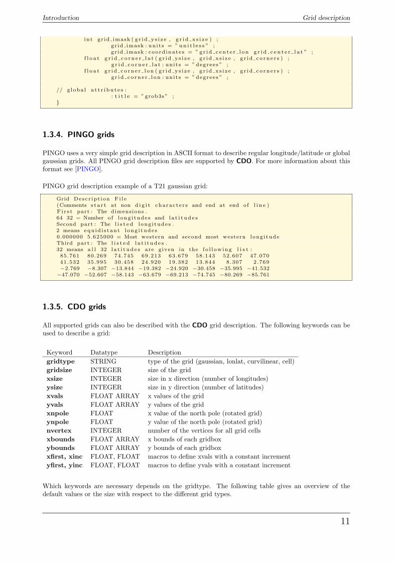
PINGO uses a very simple grid description in ASCII format to describe regular longitude/latitude or globalgaussian grids. All PINGO grid description files are supported by CDO. For more information about thisformat see [PINGO].
PINGO grid description example of a T21 gaussian grid:
Grid Desc r ip t i on F i l e(Comments s t a r t at non d i g i t cha ra c t e r s and end at end o f l i n e )F i r s t part : The dimensions .64 32 = Number o f l ong i tude s and l a t i t u d e sSecond part : The l i s t e d l ong i tude s .2 means equ i d i s t an t l ong i tude s0 .000000 5.625000 = Most western and second most western l ong i tudeThird part : The l i s t e d l a t i t u d e s .32 means a l l 32 l a t i t u d e s are g iven in the f o l l ow i n g l i s t :85 .761 80 .269 74 .745 69 .213 63 .679 58 .143 52 .607 47 .07041 .532 35 .995 30 .458 24 .920 19 .382 13 .844 8 .307 2 .769−2.769 −8.307 −13.844 −19.382 −24.920 −30.458 −35.995 −41.532
−47.070 −52.607 −58.143 −63.679 −69.213 −74.745 −80.269 −85.761
1.3.5. CDO grids
All supported grids can also be described with the CDO grid description. The following keywords can beused to describe a grid:
Keyword Datatype Descriptiongridtype STRING type of the grid (gaussian, lonlat, curvilinear, cell)gridsize INTEGER size of the gridxsize INTEGER size in x direction (number of longitudes)ysize INTEGER size in y direction (number of latitudes)xvals FLOAT ARRAY x values of the gridyvals FLOAT ARRAY y values of the gridxnpole FLOAT x value of the north pole (rotated grid)ynpole FLOAT y value of the north pole (rotated grid)nvertex INTEGER number of the vertices for all grid cellsxbounds FLOAT ARRAY x bounds of each gridboxybounds FLOAT ARRAY y bounds of each gridboxxfirst, xinc FLOAT, FLOAT macros to define xvals with a constant incrementyfirst, yinc FLOAT, FLOAT macros to define yvals with a constant increment
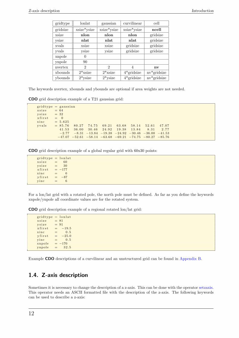
Which keywords are necessary depends on the gridtype. The following table gives an overview of thedefault values or the size with respect to the different grid types.
11
Z-axis description Introduction
gridtype lonlat gaussian curvilinear cell
gridsize xsize*ysize xsize*ysize xsize*ysize ncellxsize nlon nlon nlon gridsizeysize nlat nlat nlat gridsizexvals xsize xsize gridsize gridsizeyvals ysize ysize gridsize gridsizexnpole 0ynpole 90nvertex 2 2 4 nvxbounds 2*xsize 2*xsize 4*gridsize nv*gridsizeybounds 2*ysize 2*ysize 4*gridsize nv*gridsize
The keywords nvertex, xbounds and ybounds are optional if area weights are not needed.
CDO grid description example of a T21 gaussian grid:
gr id type = gauss ianx s i z e = 64y s i z e = 32x f i r s t = 0xinc = 5.625yva l s = 85 .76 80 .27 74 .75 69 .21 63 .68 58 .14 52 .61 47 .07
41 .53 36 .00 30 .46 24 .92 19 .38 13 .84 8 .31 2 .77−2.77 −8.31 −13.84 −19.38 −24.92 −30.46 −36.00 −41.53−47.07 −52.61 −58.14 −63.68 −69.21 −74.75 −80.27 −85.76
CDO grid description example of a global regular grid with 60x30 points:
gr id type = l o n l a tx s i z e = 60y s i z e = 30x f i r s t = −177xinc = 6y f i r s t = −87yinc = 6
For a lon/lat grid with a rotated pole, the north pole must be defined. As far as you define the keywordsxnpole/ynpole all coordinate values are for the rotated system.
CDO grid description example of a regional rotated lon/lat grid:
gr id type = l o n l a tx s i z e = 81y s i z e = 91x f i r s t = −19.5x inc = 0 .5y f i r s t = −25.0y inc = 0 .5xnpole = −170ynpole = 32 .5
Example CDO descriptions of a curvilinear and an unstructured grid can be found in Appendix B.
1.4. Z-axis description
Sometimes it is necessary to change the description of a z-axis. This can be done with the operator setzaxis.This operator needs an ASCII formatted file with the description of the z-axis. The following keywordscan be used to describe a z-axis:
12
Introduction Time axis
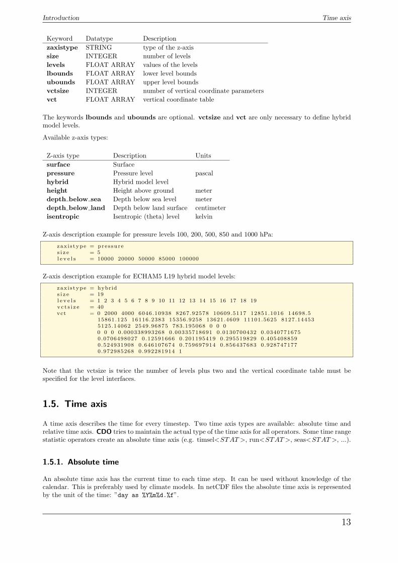
Keyword Datatype Descriptionzaxistype STRING type of the z-axissize INTEGER number of levelslevels FLOAT ARRAY values of the levelslbounds FLOAT ARRAY lower level boundsubounds FLOAT ARRAY upper level boundsvctsize INTEGER number of vertical coordinate parametersvct FLOAT ARRAY vertical coordinate table
The keywords lbounds and ubounds are optional. vctsize and vct are only necessary to define hybridmodel levels.
Available z-axis types:
Z-axis type Description Unitssurface Surfacepressure Pressure level pascalhybrid Hybrid model levelheight Height above ground meterdepth below sea Depth below sea level meterdepth below land Depth below land surface centimeterisentropic Isentropic (theta) level kelvin
Z-axis description example for pressure levels 100, 200, 500, 850 and 1000 hPa:
zax i s type = pre s su r es i z e = 5l e v e l s = 10000 20000 50000 85000 100000
Z-axis description example for ECHAM5 L19 hybrid model levels:
zax i s type = hybrids i z e = 19l e v e l s = 1 2 3 4 5 6 7 8 9 10 11 12 13 14 15 16 17 18 19v c t s i z e = 40vct = 0 2000 4000 6046.10938 8267.92578 10609.5117 12851.1016 14698.5
15861.125 16116.2383 15356.9258 13621.4609 11101.5625 8127.144535125.14062 2549.96875 783.195068 0 0 00 0 0 0.000338993268 0.00335718691 0.0130700432 0.03407716750.0706498027 0.12591666 0.201195419 0.295519829 0.4054088590.524931908 0.646107674 0.759697914 0.856437683 0.9287471770.972985268 0.992281914 1
Note that the vctsize is twice the number of levels plus two and the vertical coordinate table must bespecified for the level interfaces.
1.5. Time axis
A time axis describes the time for every timestep. Two time axis types are available: absolute time andrelative time axis. CDO tries to maintain the actual type of the time axis for all operators. Some time rangestatistic operators create an absolute time axis (e.g. timsel<STAT >, run<STAT >, seas<STAT >, ...).
1.5.1. Absolute time
An absolute time axis has the current time to each time step. It can be used without knowledge of thecalendar. This is preferably used by climate models. In netCDF files the absolute time axis is representedby the unit of the time: ”day as %Y%m%d.%f”.
13
Parameter table Introduction
1.5.2. Relative time
A relative time is the time relative to a fixed reference time. The current time results from the referencetime and the elapsed interval. The result depends on the calendar used. CDO supports the standardGregorian, 360 days, 365 days and 366 days calendars. The relative time axis is preferably used by weatherforecast models. In netCDF files the relative time axis is represented by the unit of the time: ”time-unitssince reference-time”, e.g ”days since 1989-6-15 12:00”.
1.5.3. Conversion of the time
Some programs which work with netCDF data can only process relative time axes. Therefore it may benecessary to convert from an absolute into a relative time axis. This conversion can be done for eachoperator with the CDO option ’-r’. To convert a relative into an absolute time axis use the CDO option’-a’.
1.6. Parameter table
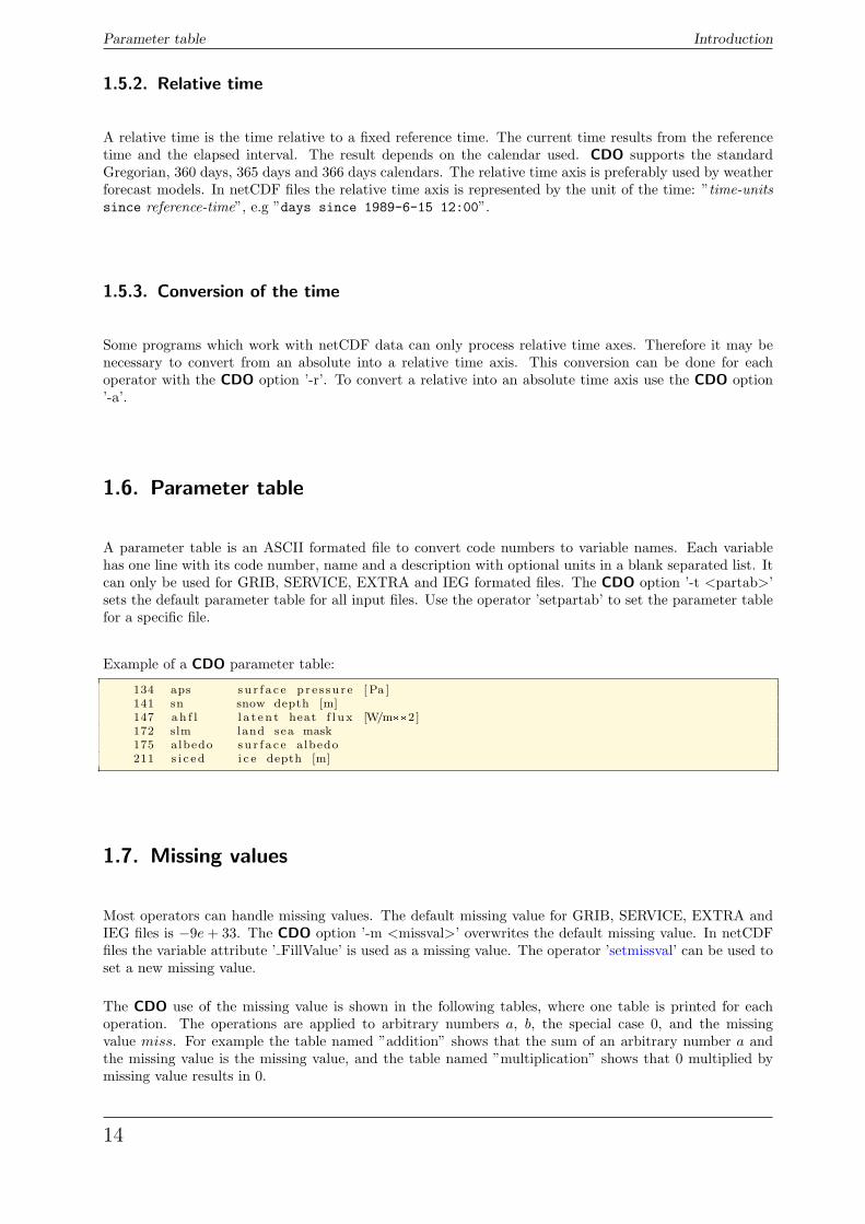
A parameter table is an ASCII formated file to convert code numbers to variable names. Each variablehas one line with its code number, name and a description with optional units in a blank separated list. Itcan only be used for GRIB, SERVICE, EXTRA and IEG formated files. The CDO option ’-t <partab>’sets the default parameter table for all input files. Use the operator ’setpartab’ to set the parameter tablefor a specific file.
Example of a CDO parameter table:
134 aps su r f a c e p r e s su r e [ Pa ]141 sn snow depth [m]147 ah f l l a t e n t heat f l u x [W/m**2 ]172 slm land sea mask175 albedo su r f a c e albedo211 s i c e d i c e depth [m]
1.7. Missing values
Most operators can handle missing values. The default missing value for GRIB, SERVICE, EXTRA andIEG files is −9e + 33. The CDO option ’-m <missval>’ overwrites the default missing value. In netCDFfiles the variable attribute ’ FillValue’ is used as a missing value. The operator ’setmissval’ can be used toset a new missing value.
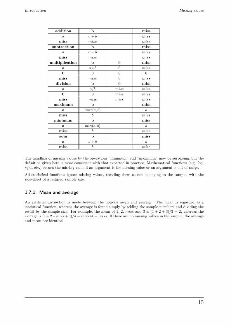
The CDO use of the missing value is shown in the following tables, where one table is printed for eachoperation. The operations are applied to arbitrary numbers a, b, the special case 0, and the missingvalue miss. For example the table named ”addition” shows that the sum of an arbitrary number a andthe missing value is the missing value, and the table named ”multiplication” shows that 0 multiplied bymissing value results in 0.
14
Introduction Missing values
addition b missa a + b miss
miss miss miss
subtraction b missa a− b miss
miss miss miss
multiplication b 0 missa a ∗ b 0 miss
0 0 0 0miss miss 0 miss
division b 0 missa a/b miss miss
0 0 miss miss
miss miss miss miss
maximum b missa max(a, b) a
miss b miss
minimum b missa min(a, b) a
miss b miss
sum b missa a + b a
miss b miss
The handling of missing values by the operations ”minimum” and ”maximum” may be surprising, but thedefinition given here is more consistent with that expected in practice. Mathematical functions (e.g. log,sqrt, etc.) return the missing value if an argument is the missing value or an argument is out of range.
All statistical functions ignore missing values, treading them as not belonging to the sample, with theside-effect of a reduced sample size.
1.7.1. Mean and average
An artificial distinction is made between the notions mean and average. The mean is regarded as astatistical function, whereas the average is found simply by adding the sample members and dividing theresult by the sample size. For example, the mean of 1, 2, miss and 3 is (1 + 2 + 3)/3 = 2, whereas theaverage is (1+2+miss+3)/4 = miss/4 = miss. If there are no missing values in the sample, the averageand mean are identical.
15
2. Reference manual
This section gives a description of all operators. Related operators are grouped to modules. For easierdescription all single input files are named ifile or ifile1, ifile2, etc., and an unlimited number ofinput files are named ifiles. All output files are named ofile or ofile1, ofile2, etc. Further thefollowing notion is introduced:
i(t) Timestep t of ifile
i(t, x) Element number x of the field at timestep t of ifile
o(t) Timestep t of ofile
o(t, x) Element number x of the field at timestep t of ofile
16
Reference manual Information
2.1. Information
This section contains modules to print information about datasets. All operators print there results tostandard output.
Here is a short overview of all operators in this section:
info Dataset information listed by code numberinfov Dataset information listed by variable namemap Dataset information and simple map
sinfo Short dataset information listed by code numbersinfov Short dataset information listed by variable name
diff Compare two datasets listed by code numberdiffv Compare two datasets listed by variable name
npar Number of parametersnlevel Number of levelsnyear Number of yearsnmon Number of monthsndate Number of datesntime Number of time steps
showformat Show file formatshowcode Show code numbersshowname Show variable namesshowstdname Show standard namesshowlevel Show levelsshowltype Show GRIB level typesshowyear Show yearsshowmon Show monthsshowdate Show date informationshowtime Show time informationshowtimestamp Show timestamp
pardes Parameter descriptiongriddes Grid descriptionzaxisdes Z-axis descriptionvct Vertical coordinate table
17
Information Reference manual
2.1.1. INFO - Information and simple statistics
Synopsis
<operator> ifiles
Description
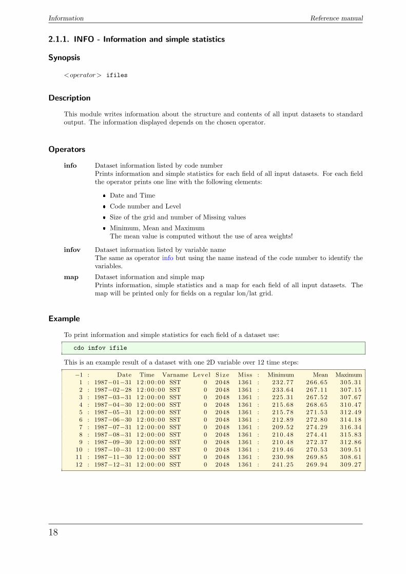
This module writes information about the structure and contents of all input datasets to standardoutput. The information displayed depends on the chosen operator.
Operators
info Dataset information listed by code numberPrints information and simple statistics for each field of all input datasets. For each fieldthe operator prints one line with the following elements:
� Date and Time
� Code number and Level
� Size of the grid and number of Missing values
� Minimum, Mean and MaximumThe mean value is computed without the use of area weights!
infov Dataset information listed by variable nameThe same as operator info but using the name instead of the code number to identify thevariables.
map Dataset information and simple mapPrints information, simple statistics and a map for each field of all input datasets. Themap will be printed only for fields on a regular lon/lat grid.
Example
To print information and simple statistics for each field of a dataset use:
cdo infov ifile
This is an example result of a dataset with one 2D variable over 12 time steps:
−1 : Date Time Varname Level S i z e Miss : Minimum Mean Maximum1 : 1987−01−31 12 : 00 : 00 SST 0 2048 1361 : 232 .77 266 .65 305 .312 : 1987−02−28 12 : 00 : 00 SST 0 2048 1361 : 233 .64 267 .11 307 .153 : 1987−03−31 12 : 00 : 00 SST 0 2048 1361 : 225 .31 267 .52 307 .674 : 1987−04−30 12 : 00 : 00 SST 0 2048 1361 : 215 .68 268 .65 310 .475 : 1987−05−31 12 : 00 : 00 SST 0 2048 1361 : 215 .78 271 .53 312 .496 : 1987−06−30 12 : 00 : 00 SST 0 2048 1361 : 212 .89 272 .80 314 .187 : 1987−07−31 12 : 00 : 00 SST 0 2048 1361 : 209 .52 274 .29 316 .348 : 1987−08−31 12 : 00 : 00 SST 0 2048 1361 : 210 .48 274 .41 315 .839 : 1987−09−30 12 : 00 : 00 SST 0 2048 1361 : 210 .48 272 .37 312 .86
10 : 1987−10−31 12 : 00 : 00 SST 0 2048 1361 : 219 .46 270 .53 309 .5111 : 1987−11−30 12 : 00 : 00 SST 0 2048 1361 : 230 .98 269 .85 308 .6112 : 1987−12−31 12 : 00 : 00 SST 0 2048 1361 : 241 .25 269 .94 309 .27
18
Reference manual Information
2.1.2. SINFO - Short information
Synopsis
<operator> ifiles
Description
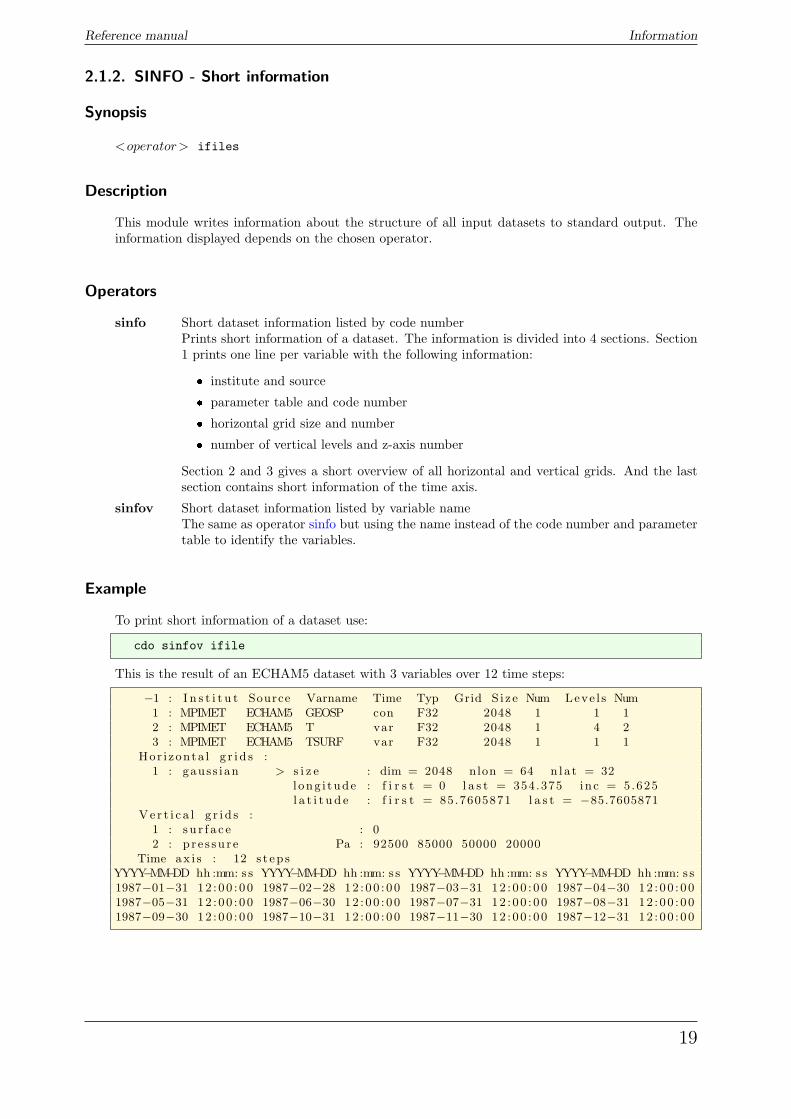
This module writes information about the structure of all input datasets to standard output. Theinformation displayed depends on the chosen operator.
Operators
sinfo Short dataset information listed by code numberPrints short information of a dataset. The information is divided into 4 sections. Section1 prints one line per variable with the following information:
� institute and source
� parameter table and code number
� horizontal grid size and number
� number of vertical levels and z-axis number
Section 2 and 3 gives a short overview of all horizontal and vertical grids. And the lastsection contains short information of the time axis.
sinfov Short dataset information listed by variable nameThe same as operator sinfo but using the name instead of the code number and parametertable to identify the variables.
Example
To print short information of a dataset use:
cdo sinfov ifile
This is the result of an ECHAM5 dataset with 3 variables over 12 time steps:
−1 : I n s t i t u t Source Varname Time Typ Grid S i z e Num Leve l s Num1 : MPIMET ECHAM5 GEOSP con F32 2048 1 1 12 : MPIMET ECHAM5 T var F32 2048 1 4 23 : MPIMET ECHAM5 TSURF var F32 2048 1 1 1
Hor i zonta l g r i d s :1 : gauss ian > s i z e : dim = 2048 nlon = 64 n la t = 32
l ong i tude : f i r s t = 0 l a s t = 354.375 inc = 5.625l a t i t u d e : f i r s t = 85.7605871 l a s t = −85.7605871
Ve r t i c a l g r i d s :1 : s u r f a c e : 02 : p r e s su r e Pa : 92500 85000 50000 20000
Time ax i s : 12 s t ep sYYYY−MM−DD hh :mm: s s YYYY−MM−DD hh :mm: s s YYYY−MM−DD hh :mm: s s YYYY−MM−DD hh :mm: s s1987−01−31 12 : 00 : 00 1987−02−28 12 : 00 : 00 1987−03−31 12 : 00 : 00 1987−04−30 12 : 00 : 001987−05−31 12 : 00 : 00 1987−06−30 12 : 00 : 00 1987−07−31 12 : 00 : 00 1987−08−31 12 : 00 : 001987−09−30 12 : 00 : 00 1987−10−31 12 : 00 : 00 1987−11−30 12 : 00 : 00 1987−12−31 12 : 00 : 00
19
Information Reference manual
2.1.3. DIFF - Compare two datasets field by field
Synopsis
<operator> ifile1 ifile2
Description
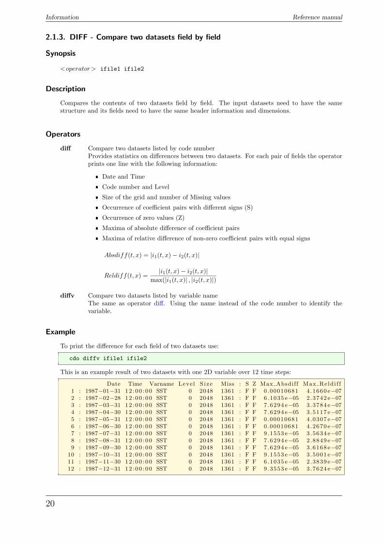
Compares the contents of two datasets field by field. The input datasets need to have the samestructure and its fields need to have the same header information and dimensions.
Operators
diff Compare two datasets listed by code numberProvides statistics on differences between two datasets. For each pair of fields the operatorprints one line with the following information:
� Date and Time
� Code number and Level
� Size of the grid and number of Missing values
� Occurrence of coefficient pairs with different signs (S)
� Occurrence of zero values (Z)
� Maxima of absolute difference of coefficient pairs
� Maxima of relative difference of non-zero coefficient pairs with equal signs
Absdiff(t, x) = |i1(t, x)− i2(t, x)|
Reldiff(t, x) =|i1(t, x)− i2(t, x)|
max(|i1(t, x)| , |i2(t, x)|)
diffv Compare two datasets listed by variable nameThe same as operator diff. Using the name instead of the code number to identify thevariable.
Example
To print the difference for each field of two datasets use:
cdo diffv ifile1 ifile2
This is an example result of two datasets with one 2D variable over 12 time steps:
Date Time Varname Level S i z e Miss : S Z Max Absdiff Max Reld i f f1 : 1987−01−31 12 : 00 : 00 SST 0 2048 1361 : F F 0.00010681 4 .1660 e−072 : 1987−02−28 12 : 00 : 00 SST 0 2048 1361 : F F 6.1035 e−05 2 .3742 e−073 : 1987−03−31 12 : 00 : 00 SST 0 2048 1361 : F F 7.6294 e−05 3 .3784 e−074 : 1987−04−30 12 : 00 : 00 SST 0 2048 1361 : F F 7.6294 e−05 3 .5117 e−075 : 1987−05−31 12 : 00 : 00 SST 0 2048 1361 : F F 0.00010681 4 .0307 e−076 : 1987−06−30 12 : 00 : 00 SST 0 2048 1361 : F F 0.00010681 4 .2670 e−077 : 1987−07−31 12 : 00 : 00 SST 0 2048 1361 : F F 9.1553 e−05 3 .5634 e−078 : 1987−08−31 12 : 00 : 00 SST 0 2048 1361 : F F 7.6294 e−05 2 .8849 e−079 : 1987−09−30 12 : 00 : 00 SST 0 2048 1361 : F F 7.6294 e−05 3 .6168 e−07
10 : 1987−10−31 12 : 00 : 00 SST 0 2048 1361 : F F 9.1553 e−05 3 .5001 e−0711 : 1987−11−30 12 : 00 : 00 SST 0 2048 1361 : F F 6.1035 e−05 2 .3839 e−0712 : 1987−12−31 12 : 00 : 00 SST 0 2048 1361 : F F 9.3553 e−05 3 .7624 e−07
20
Reference manual Information
2.1.4. NINFO - Print the number of parameters, levels or times
Synopsis
<operator> ifile
Description
This module prints the number of variables, levels or times of the input dataset.
Operators
npar Number of parametersPrints the number of parameters (variables).
nlevel Number of levelsPrints the number of levels for each variable.
nyear Number of yearsPrints the number of different years.
nmon Number of monthsPrints the number of different combinations of years and months.
ndate Number of datesPrints the number of different dates.
ntime Number of time stepsPrints the number of time steps.
Example
To print the number of parameters (variables) in a dataset use:
cdo npar ifile
To print the number of months in a dataset use:
cdo nmon ifile
21
Information Reference manual
2.1.5. SHOWINFO - Show variables, levels or times
Synopsis
<operator> ifile
Description
This module prints the format, variables, levels or times of the input dataset.
Operators
showformat Show file formatPrints the file format of the input dataset.
showcode Show code numbersPrints the code number of all variables.
showname Show variable namesPrints the name of all variables.
showstdname Show standard namesPrints the standard name of all variables.
showlevel Show levelsPrints all levels for each variable.
showltype Show GRIB level typesPrints the GRIB level type for all z-axes.
showyear Show yearsPrints all years.
showmon Show monthsPrints all months.
showdate Show date informationPrints date information of all time steps (format YYYY-MM-DD).
showtime Show time informationPrints time information of all time steps (format hh:mm:ss).
showtimestamp Show timestampPrints timestamp of all time steps (format YYYY-MM-DDThh:mm:ss).
Example
To print the code number of all variables in a dataset use:
cdo showcode ifile
This is an example result of a dataset with three variables:
129 130 139
To print all months in a dataset use:
cdo showmon ifile
This is an examples result of a dataset with an annual cycle:
1 2 3 4 5 6 7 8 9 10 11 12
22
Reference manual Information
2.1.6. FILEDES - Dataset description
Synopsis
<operator> ifile
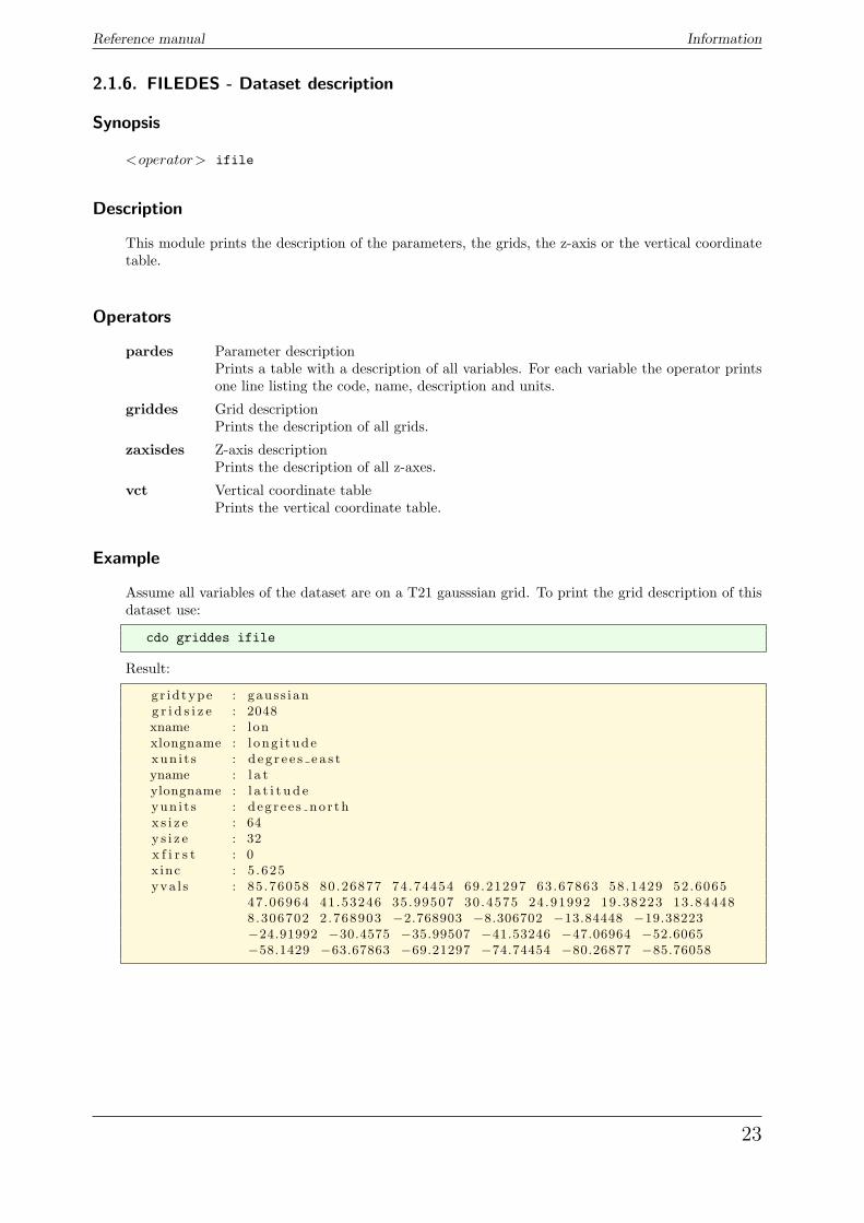
Description
This module prints the description of the parameters, the grids, the z-axis or the vertical coordinatetable.
Operators
pardes Parameter descriptionPrints a table with a description of all variables. For each variable the operator printsone line listing the code, name, description and units.
griddes Grid descriptionPrints the description of all grids.
zaxisdes Z-axis descriptionPrints the description of all z-axes.
vct Vertical coordinate tablePrints the vertical coordinate table.
Example
Assume all variables of the dataset are on a T21 gausssian grid. To print the grid description of thisdataset use:
cdo griddes ifile
Result:
gr id type : gauss iang r i d s i z e : 2048xname : lonxlongname : l ong i tudexun i t s : d e g r e e s e a s tyname : l a tylongname : l a t i t u d eyun i t s : d eg r e e s no r thx s i z e : 64y s i z e : 32x f i r s t : 0x inc : 5 .625yva l s : 85 .76058 80.26877 74.74454 69.21297 63.67863 58.1429 52.6065
47.06964 41.53246 35.99507 30.4575 24.91992 19.38223 13.844488.306702 2.768903 −2.768903 −8.306702 −13.84448 −19.38223−24.91992 −30.4575 −35.99507 −41.53246 −47.06964 −52.6065−58.1429 −63.67863 −69.21297 −74.74454 −80.26877 −85.76058
23
File operations Reference manual
2.2. File operations
This section contains modules to perform operations on files.
Here is a short overview of all operators in this section:
copy Copy datasetscat Concatenate datasets
replace Replace variables
merge Merge datasets with different fieldsmergetime Merge datasets sorted by date and time
splitcode Split code numberssplitname Split variable namessplitlevel Split levelssplitgrid Split gridssplitzaxis Split z-axessplittabnum Split parameter table numbers
splithour Split hourssplitday Split dayssplitmon Split monthssplitseas Split seasonssplityear Split years
splitsel Split time selection
24
Reference manual File operations
2.2.1. COPY - Copy datasets
Synopsis
<operator> ifiles ofile
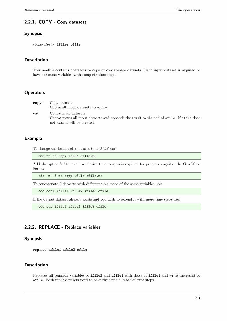
Description
This module contains operators to copy or concatenate datasets. Each input dataset is required tohave the same variables with complete time steps.
Operators
copy Copy datasetsCopies all input datasets to ofile.
cat Concatenate datasetsConcatenates all input datasets and appends the result to the end of ofile. If ofile doesnot exist it will be created.
Example
To change the format of a dataset to netCDF use:
cdo -f nc copy ifile ofile.nc
Add the option ’-r’ to create a relative time axis, as is required for proper recognition by GrADS orFerret:
cdo -r -f nc copy ifile ofile.nc
To concatenate 3 datasets with different time steps of the same variables use:
cdo copy ifile1 ifile2 ifile3 ofile
If the output dataset already exists and you wish to extend it with more time steps use:
cdo cat ifile1 ifile2 ifile3 ofile
2.2.2. REPLACE - Replace variables
Synopsis
replace ifile1 ifile2 ofile
Description
Replaces all common variables of ifile2 and ifile1 with those of ifile1 and write the result toofile. Both input datasets need to have the same number of time steps.
25

File operations Reference manual
Example
Assume the first input dataset ifile1 has three variables with the names geosp, t and tslm1 and thesecond input dataset ifile2 has only the variable tslm1. To replace the variable tslm1 in ifile1with tslm1 from ifile2 use:
cdo replace ifile1 ifile2 ofile
26
Reference manual File operations
2.2.3. MERGE - Merge datasets
Synopsis
<operator> ifiles ofile
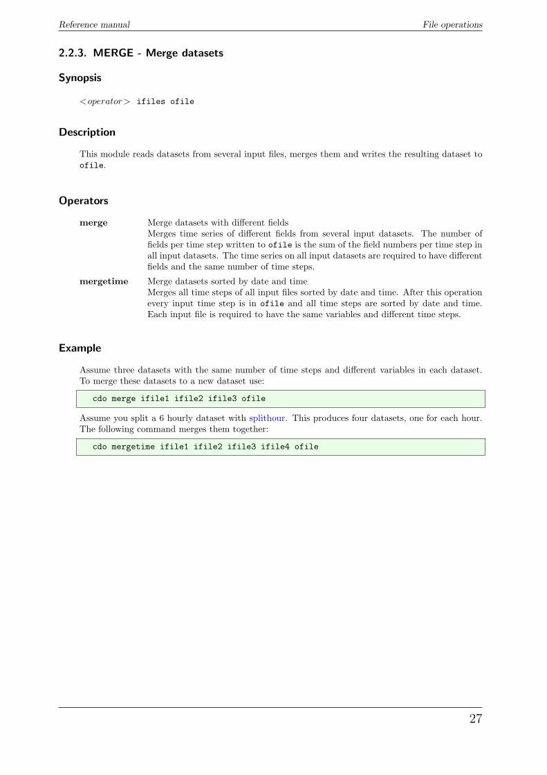
Description
This module reads datasets from several input files, merges them and writes the resulting dataset toofile.
Operators
merge Merge datasets with different fieldsMerges time series of different fields from several input datasets. The number offields per time step written to ofile is the sum of the field numbers per time step inall input datasets. The time series on all input datasets are required to have differentfields and the same number of time steps.
mergetime Merge datasets sorted by date and timeMerges all time steps of all input files sorted by date and time. After this operationevery input time step is in ofile and all time steps are sorted by date and time.Each input file is required to have the same variables and different time steps.
Example
Assume three datasets with the same number of time steps and different variables in each dataset.To merge these datasets to a new dataset use:
cdo merge ifile1 ifile2 ifile3 ofile
Assume you split a 6 hourly dataset with splithour. This produces four datasets, one for each hour.The following command merges them together:
cdo mergetime ifile1 ifile2 ifile3 ifile4 ofile
27
File operations Reference manual
2.2.4. SPLIT - Split a dataset
Synopsis
<operator> ifile obase
Description
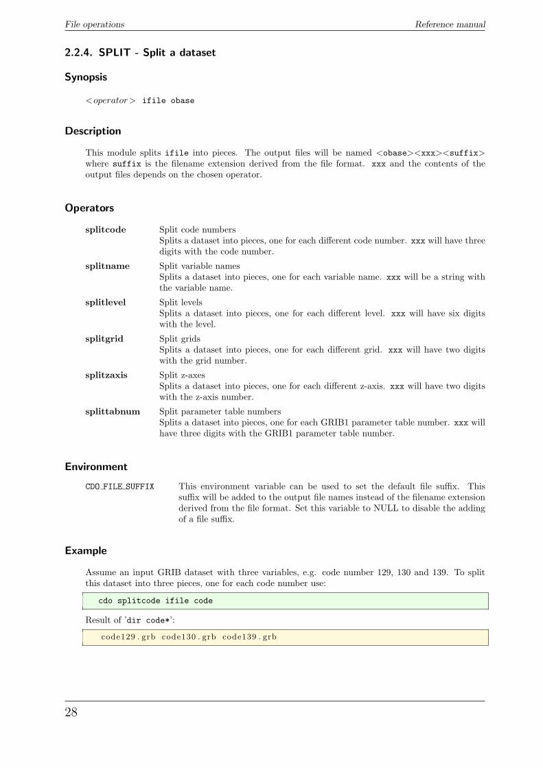
This module splits ifile into pieces. The output files will be named <obase><xxx><suffix>where suffix is the filename extension derived from the file format. xxx and the contents of theoutput files depends on the chosen operator.
Operators
splitcode Split code numbersSplits a dataset into pieces, one for each different code number. xxx will have threedigits with the code number.
splitname Split variable namesSplits a dataset into pieces, one for each variable name. xxx will be a string withthe variable name.
splitlevel Split levelsSplits a dataset into pieces, one for each different level. xxx will have six digitswith the level.
splitgrid Split gridsSplits a dataset into pieces, one for each different grid. xxx will have two digitswith the grid number.
splitzaxis Split z-axesSplits a dataset into pieces, one for each different z-axis. xxx will have two digitswith the z-axis number.
splittabnum Split parameter table numbersSplits a dataset into pieces, one for each GRIB1 parameter table number. xxx willhave three digits with the GRIB1 parameter table number.
Environment
CDO FILE SUFFIX This environment variable can be used to set the default file suffix. Thissuffix will be added to the output file names instead of the filename extensionderived from the file format. Set this variable to NULL to disable the addingof a file suffix.
Example
Assume an input GRIB dataset with three variables, e.g. code number 129, 130 and 139. To splitthis dataset into three pieces, one for each code number use:
cdo splitcode ifile code
Result of ’dir code*’:
code129 . grb code130 . grb code139 . grb
28
Reference manual File operations
2.2.5. SPLITTIME - Split time steps of a dataset
Synopsis
<operator> ifile obase
Description
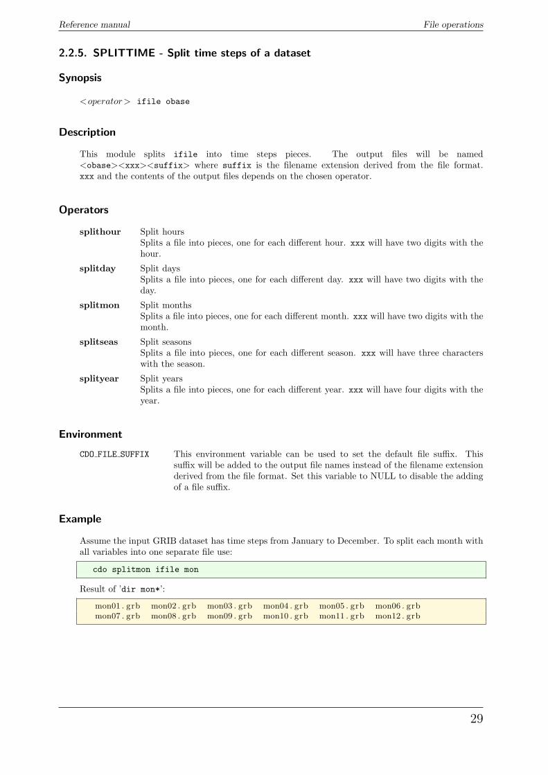
This module splits ifile into time steps pieces. The output files will be named<obase><xxx><suffix> where suffix is the filename extension derived from the file format.xxx and the contents of the output files depends on the chosen operator.
Operators
splithour Split hoursSplits a file into pieces, one for each different hour. xxx will have two digits with thehour.
splitday Split daysSplits a file into pieces, one for each different day. xxx will have two digits with theday.
splitmon Split monthsSplits a file into pieces, one for each different month. xxx will have two digits with themonth.
splitseas Split seasonsSplits a file into pieces, one for each different season. xxx will have three characterswith the season.
splityear Split yearsSplits a file into pieces, one for each different year. xxx will have four digits with theyear.
Environment
CDO FILE SUFFIX This environment variable can be used to set the default file suffix. Thissuffix will be added to the output file names instead of the filename extensionderived from the file format. Set this variable to NULL to disable the addingof a file suffix.
Example
Assume the input GRIB dataset has time steps from January to December. To split each month withall variables into one separate file use:
cdo splitmon ifile mon
Result of ’dir mon*’:
mon01 . grb mon02 . grb mon03 . grb mon04 . grb mon05 . grb mon06 . grbmon07 . grb mon08 . grb mon09 . grb mon10 . grb mon11 . grb mon12 . grb
29
File operations Reference manual
2.2.6. SPLITSEL - Split selected time steps
Synopsis
splitsel,nsets[,noffset[,nskip]] ifile obase
Description
This operator splits ifile into pieces, one for each adjacent sequence t1, ...., tn of time steps ofthe same selected time range. The output files will be named <obase><nnnnnn><suffix> wherennnnnn is the sequence number and suffix is the filename extension derived from the file format.
Parameter
nsets INTEGER Number of input time steps for each output file
noffset INTEGER Number of input time steps skipped before the first time step range (optional)
nskip INTEGER Number of input time steps skipped between time step ranges (optional)
Environment
CDO FILE SUFFIX This environment variable can be used to set the default file suffix. Thissuffix will be added to the output file names instead of the filename extensionderived from the file format. Set this variable to NULL to disable the addingof a file suffix.
30
Reference manual Selection
2.3. Selection
This section contains modules to select time steps, fields or a part of a field from a dataset.
Here is a short overview of all operators in this section:
selcode Select variables by code numberdelcode Delete variables by code numberselname Select variables by namedelname Delete variables by nameselstdname Select variables by standard namesellevel Select levelssellevidx Select levels by indexselgrid Select gridsselzaxis Select z-axesselltype Select GRIB level typesseltabnum Select parameter table numbers
seltimestep Select time stepsseltime Select timesselhour Select hoursselday Select daysselmon Select monthsselyear Select yearsselseas Select seasonsseldate Select datesselsmon Select single month
sellonlatbox Select a longitude/latitude boxselindexbox Select an index box
31
Selection Reference manual
2.3.1. SELVAR - Select fields
Synopsis
selcode,codes ifile ofile
delcode,codes ifile ofile
selname,varnames ifile ofile
delname,varnames ifile ofile
selstdname,stdnames ifile ofile
sellevel,levels ifile ofile
sellevidx,levidx ifile ofile
selgrid,grids ifile ofile
selzaxis,zaxes ifile ofile
selltype,ltypes ifile ofile
seltabnum,tabnums ifile ofile
Description
This module selects some fields from ifile and writes them to ofile. The fields selected depend onthe chosen operator and the parameters.
Operators
selcode Select variables by code numberSelects all fields with code numbers in a user given list.
delcode Delete variables by code numberDeletes all fields with code numbers in a user given list.
selname Select variables by nameSelects all fields with variable names in a user given list.
delname Delete variables by nameDeletes all fields with variable names in a user given list.
selstdname Select variables by standard nameSelects all fields with standard names in a user given list.
sellevel Select levelsSelects all fields with levels in a user given list.
sellevidx Select levels by indexSelects all fields with index of levels in a user given list.
selgrid Select gridsSelects all fields with grids in a user given list.
selzaxis Select z-axesSelects all fields with z-axes in a user given list.
selltype Select GRIB level typesSelects all fields with GRIB level type in a user given list.
seltabnum Select parameter table numbersSelects all fields with parameter table numbers in a user given list.
32
Reference manual Selection
Parameter
codes INTEGER Comma separated list of code numbers
varnames STRING Comma separated list of variable names
stdnames STRING Comma separated list of standard names
levels FLOAT Comma separated list of levels
levidx INTEGER Comma separated list of index of levels
ltypes INTEGER Comma separated list of GRIB level types
grids STRING Comma separated list of grid names or numbers
zaxes STRING Comma separated list of z-axis names or numbers
tabnums INTEGER Comma separated list of parameter table numbers
Example
Assume an input dataset has three variables with the code numbers 129, 130 and 139. To select thevariables with the code number 129 and 139 use:
cdo selcode,129,139 ifile ofile
You can also select the code number 129 and 139 by deleting the code number 130 with:
cdo delcode,130 ifile ofile
33
Selection Reference manual
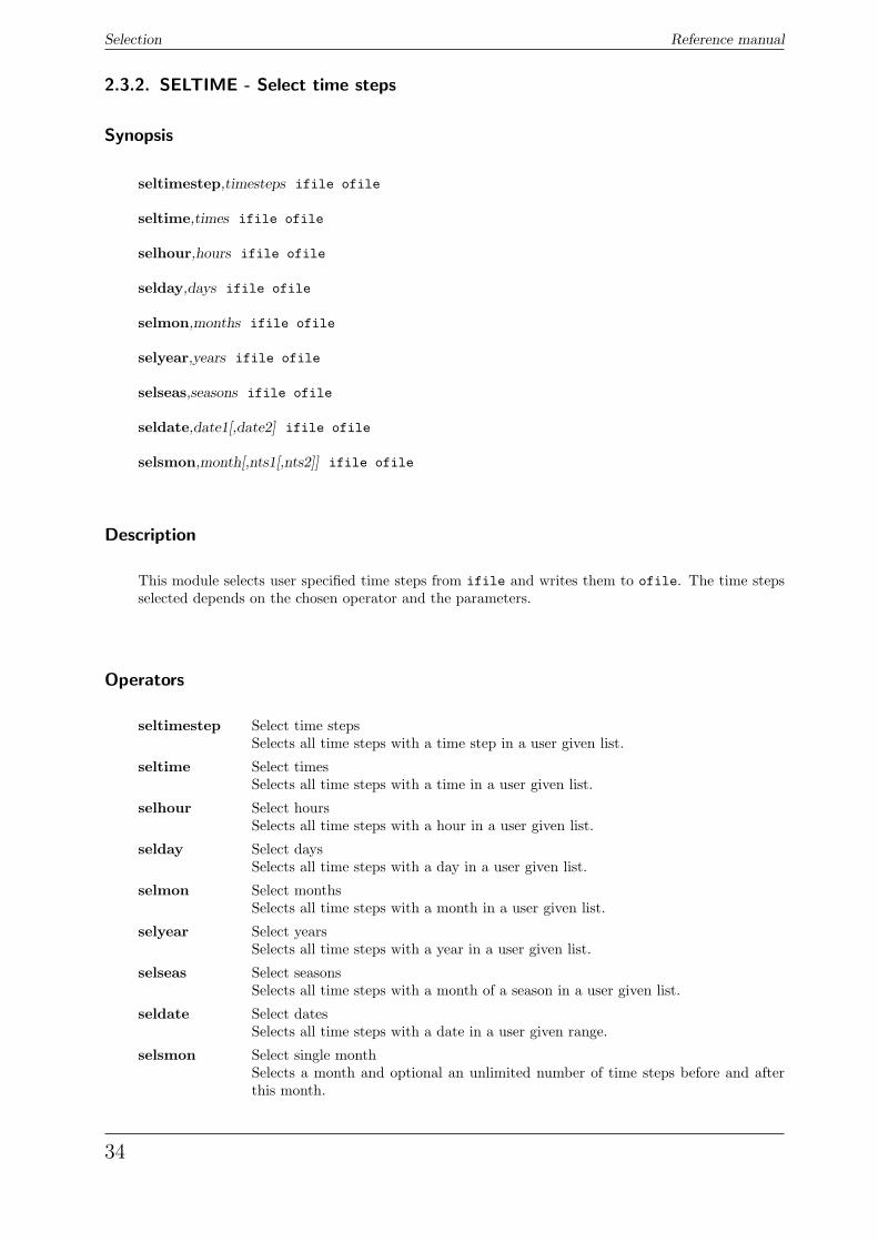
2.3.2. SELTIME - Select time steps
Synopsis
seltimestep,timesteps ifile ofile
seltime,times ifile ofile
selhour,hours ifile ofile
selday,days ifile ofile
selmon,months ifile ofile
selyear,years ifile ofile
selseas,seasons ifile ofile
seldate,date1[,date2] ifile ofile
selsmon,month[,nts1[,nts2]] ifile ofile
Description
This module selects user specified time steps from ifile and writes them to ofile. The time stepsselected depends on the chosen operator and the parameters.
Operators
seltimestep Select time stepsSelects all time steps with a time step in a user given list.
seltime Select timesSelects all time steps with a time in a user given list.
selhour Select hoursSelects all time steps with a hour in a user given list.
selday Select daysSelects all time steps with a day in a user given list.
selmon Select monthsSelects all time steps with a month in a user given list.
selyear Select yearsSelects all time steps with a year in a user given list.
selseas Select seasonsSelects all time steps with a month of a season in a user given list.
seldate Select datesSelects all time steps with a date in a user given range.
selsmon Select single monthSelects a month and optional an unlimited number of time steps before and afterthis month.
34
Reference manual Selection
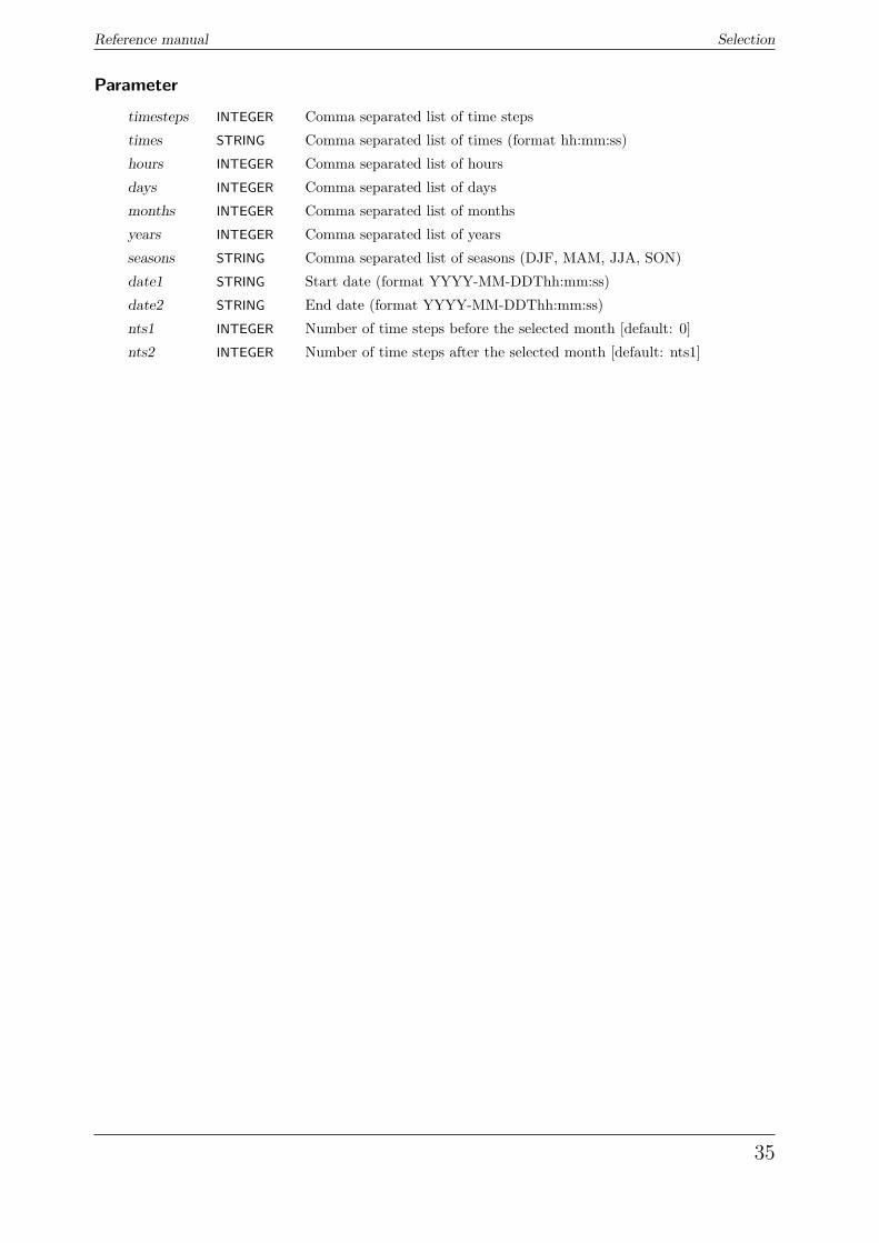
Parameter
timesteps INTEGER Comma separated list of time steps
times STRING Comma separated list of times (format hh:mm:ss)
hours INTEGER Comma separated list of hours
days INTEGER Comma separated list of days
months INTEGER Comma separated list of months
years INTEGER Comma separated list of years
seasons STRING Comma separated list of seasons (DJF, MAM, JJA, SON)
date1 STRING Start date (format YYYY-MM-DDThh:mm:ss)
date2 STRING End date (format YYYY-MM-DDThh:mm:ss)
nts1 INTEGER Number of time steps before the selected month [default: 0]
nts2 INTEGER Number of time steps after the selected month [default: nts1]
35
Selection Reference manual
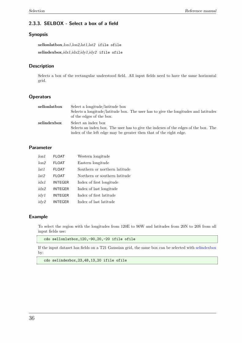
2.3.3. SELBOX - Select a box of a field
Synopsis
sellonlatbox,lon1,lon2,lat1,lat2 ifile ofile
selindexbox,idx1,idx2,idy1,idy2 ifile ofile
Description
Selects a box of the rectangular understood field. All input fields need to have the same horizontalgrid.
Operators
sellonlatbox Select a longitude/latitude boxSelects a longitude/latitude box. The user has to give the longitudes and latitudesof the edges of the box.
selindexbox Select an index boxSelects an index box. The user has to give the indexes of the edges of the box. Theindex of the left edge may be greater then that of the right edge.
Parameter
lon1 FLOAT Western longitude
lon2 FLOAT Eastern longitude
lat1 FLOAT Southern or northern latitude
lat2 FLOAT Northern or southern latitude
idx1 INTEGER Index of first longitude
idx2 INTEGER Index of last longitude
idy1 INTEGER Index of first latitude
idy2 INTEGER Index of last latitude
Example
To select the region with the longitudes from 120E to 90W and latitudes from 20N to 20S from allinput fields use:
cdo sellonlatbox,120,-90,20,-20 ifile ofile
If the input dataset has fields on a T21 Gaussian grid, the same box can be selected with selindexboxby:
cdo selindexbox,23,48,13,20 ifile ofile
36
Reference manual Conditional selection
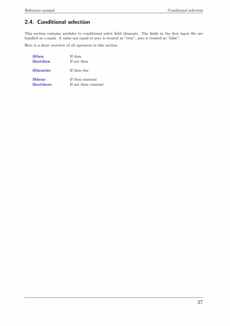
2.4. Conditional selection
This section contains modules to conditional select field elements. The fields in the first input file arehandled as a mask. A value not equal to zero is treated as ”true”, zero is treated as ”false”.
Here is a short overview of all operators in this section:
ifthen If thenifnotthen If not then
ifthenelse If then else
ifthenc If then constantifnotthenc If not then constant
37
Conditional selection Reference manual
2.4.1. COND - Conditional select one field
Synopsis
<operator> ifile1 ifile2 ofile
Description
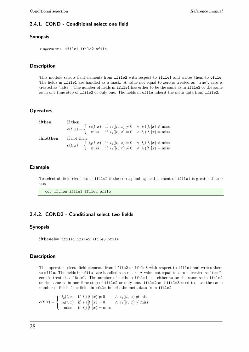
This module selects field elements from ifile2 with respect to ifile1 and writes them to ofile.The fields in ifile1 are handled as a mask. A value not equal to zero is treated as ”true”, zero istreated as ”false”. The number of fields in ifile1 has either to be the same as in ifile2 or the sameas in one time step of ifile2 or only one. The fields in ofile inherit the meta data from ifile2.
Operators
ifthen If then
o(t, x) ={
i2(t, x) if i1([t, ]x) 6= 0 ∧ i1([t, ]x) 6= missmiss if i1([t, ]x) = 0 ∨ i1([t, ]x) = miss
ifnotthen If not then
o(t, x) ={
i2(t, x) if i1([t, ]x) = 0 ∧ i1([t, ]x) 6= missmiss if i1([t, ]x) 6= 0 ∨ i1([t, ]x) = miss
Example
To select all field elements of ifile2 if the corresponding field element of ifile1 is greater than 0use:
cdo ifthen ifile1 ifile2 ofile
2.4.2. COND2 - Conditional select two fields
Synopsis
ifthenelse ifile1 ifile2 ifile3 ofile
Description
This operator selects field elements from ifile2 or ifile3 with respect to ifile1 and writes themto ofile. The fields in ifile1 are handled as a mask. A value not equal to zero is treated as ”true”,zero is treated as ”false”. The number of fields in ifile1 has either to be the same as in ifile2or the same as in one time step of ifile2 or only one. ifile2 and ifile3 need to have the samenumber of fields. The fields in ofile inherit the meta data from ifile2.
o(t, x) =
i2(t, x) if i1([t, ]x) 6= 0 ∧ i1([t, ]x) 6= missi3(t, x) if i1([t, ]x) = 0 ∧ i1([t, ]x) 6= missmiss if i1([t, ]x) = miss
38

Reference manual Conditional selection
Example
To select all field elements of ifile2 if the corresponding field element of ifile1 is greater than 0and from ifile3 otherwise use:
cdo ifthenelse ifile1 ifile2 ifile3 ofile
39
Conditional selection Reference manual
2.4.3. CONDC - Conditional select a constant
Synopsis
<operator>,c ifile ofile
Description
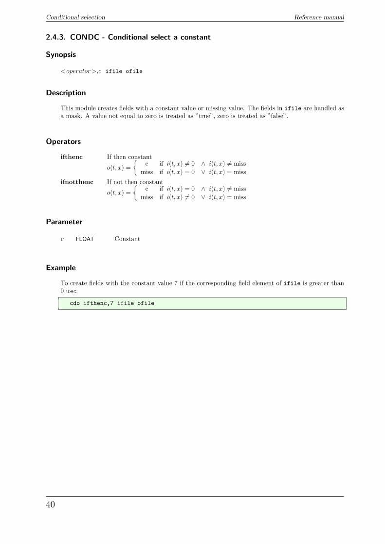
This module creates fields with a constant value or missing value. The fields in ifile are handled asa mask. A value not equal to zero is treated as ”true”, zero is treated as ”false”.
Operators
ifthenc If then constant
o(t, x) ={
c if i(t, x) 6= 0 ∧ i(t, x) 6= missmiss if i(t, x) = 0 ∨ i(t, x) = miss
ifnotthenc If not then constant
o(t, x) ={
c if i(t, x) = 0 ∧ i(t, x) 6= missmiss if i(t, x) 6= 0 ∨ i(t, x) = miss
Parameter
c FLOAT Constant
Example
To create fields with the constant value 7 if the corresponding field element of ifile is greater than0 use:
cdo ifthenc,7 ifile ofile
40
Reference manual Comparison
2.5. Comparison
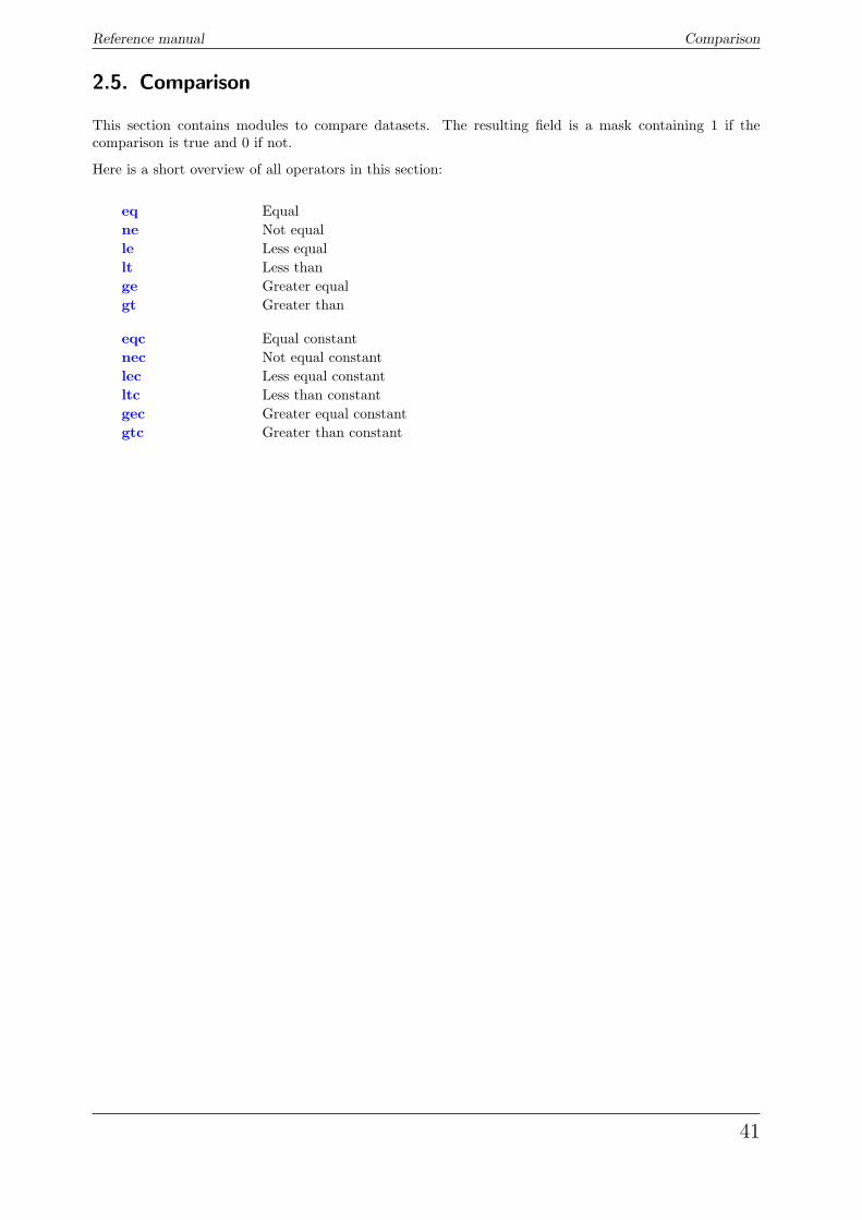
This section contains modules to compare datasets. The resulting field is a mask containing 1 if thecomparison is true and 0 if not.
Here is a short overview of all operators in this section:
eq Equalne Not equalle Less equallt Less thange Greater equalgt Greater than
eqc Equal constantnec Not equal constantlec Less equal constantltc Less than constantgec Greater equal constantgtc Greater than constant
41
Comparison Reference manual
2.5.1. COMP - Comparison of two fields
Synopsis
<operator> ifile1 ifile2 ofile
Description
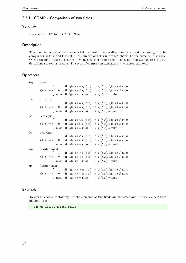
This module compares two datasets field by field. The resulting field is a mask containing 1 if thecomparison is true and 0 if not. The number of fields in ifile1 should be the same as in ifile2.One of the input files can contain only one time step or one field. The fields in ofile inherit the metadata from ifile1 or ifile2. The type of comparison depends on the chosen operator.
Operators
eq Equal
o(t, x) =
1 if i1(t, x) = i2(t, x) ∧ i1(t, x), i2(t, x) 6= miss0 if i1(t, x) 6= i2(t, x) ∧ i1(t, x), i2(t, x) 6= miss
miss if i1(t, x) = miss ∨ i2(t, x) = miss
ne Not equal
o(t, x) =
1 if i1(t, x) 6= i2(t, x) ∧ i1(t, x), i2(t, x) 6= miss0 if i1(t, x) = i2(t, x) ∧ i1(t, x), i2(t, x) 6= miss
miss if i1(t, x) = miss ∨ i2(t, x) = miss
le Less equal
o(t, x) =
1 if i1(t, x) ≤ i2(t, x) ∧ i1(t, x), i2(t, x) 6= miss0 if i1(t, x) > i2(t, x) ∧ i1(t, x), i2(t, x) 6= miss
miss if i1(t, x) = miss ∨ i2(t, x) = miss
lt Less than
o(t, x) =
1 if i1(t, x) < i2(t, x) ∧ i1(t, x), i2(t, x) 6= miss0 if i1(t, x) ≥ i2(t, x) ∧ i1(t, x), i2(t, x) 6= miss
miss if i1(t, x) = miss ∨ i2(t, x) = miss
ge Greater equal
o(t, x) =
1 if i1(t, x) ≥ i2(t, x) ∧ i1(t, x), i2(t, x) 6= miss0 if i1(t, x) < i2(t, x) ∧ i1(t, x), i2(t, x) 6= miss
miss if i1(t, x) = miss ∨ i2(t, x) = miss
gt Greater than
o(t, x) =
1 if i1(t, x) > i2(t, x) ∧ i1(t, x), i2(t, x) 6= miss0 if i1(t, x) ≤ i2(t, x) ∧ i1(t, x), i2(t, x) 6= miss
miss if i1(t, x) = miss ∨ i2(t, x) = miss
Example
To create a mask containing 1 if the elements of two fields are the same and 0 if the elements aredifferent use:
cdo eq ifile1 ifile2 ofile
42
Reference manual Comparison
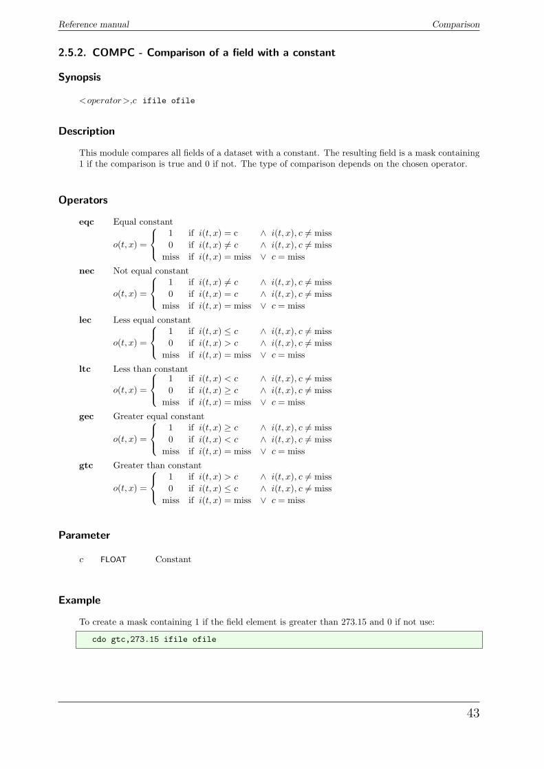
2.5.2. COMPC - Comparison of a field with a constant
Synopsis
<operator>,c ifile ofile
Description
This module compares all fields of a dataset with a constant. The resulting field is a mask containing1 if the comparison is true and 0 if not. The type of comparison depends on the chosen operator.
Operators
eqc Equal constant
o(t, x) =
1 if i(t, x) = c ∧ i(t, x), c 6= miss0 if i(t, x) 6= c ∧ i(t, x), c 6= miss
miss if i(t, x) = miss ∨ c = miss
nec Not equal constant
o(t, x) =
1 if i(t, x) 6= c ∧ i(t, x), c 6= miss0 if i(t, x) = c ∧ i(t, x), c 6= miss
miss if i(t, x) = miss ∨ c = miss
lec Less equal constant
o(t, x) =
1 if i(t, x) ≤ c ∧ i(t, x), c 6= miss0 if i(t, x) > c ∧ i(t, x), c 6= miss
miss if i(t, x) = miss ∨ c = miss
ltc Less than constant
o(t, x) =
1 if i(t, x) < c ∧ i(t, x), c 6= miss0 if i(t, x) ≥ c ∧ i(t, x), c 6= miss
miss if i(t, x) = miss ∨ c = miss
gec Greater equal constant
o(t, x) =
1 if i(t, x) ≥ c ∧ i(t, x), c 6= miss0 if i(t, x) < c ∧ i(t, x), c 6= miss
miss if i(t, x) = miss ∨ c = miss
gtc Greater than constant
o(t, x) =
1 if i(t, x) > c ∧ i(t, x), c 6= miss0 if i(t, x) ≤ c ∧ i(t, x), c 6= miss
miss if i(t, x) = miss ∨ c = miss
Parameter
c FLOAT Constant
Example
To create a mask containing 1 if the field element is greater than 273.15 and 0 if not use:
cdo gtc,273.15 ifile ofile
43
Modification Reference manual
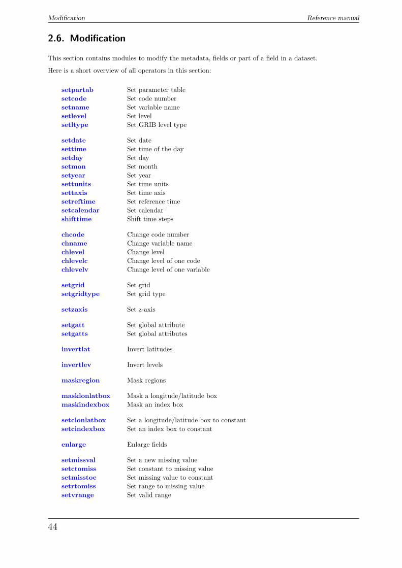
2.6. Modification
This section contains modules to modify the metadata, fields or part of a field in a dataset.
Here is a short overview of all operators in this section:
setpartab Set parameter tablesetcode Set code numbersetname Set variable namesetlevel Set levelsetltype Set GRIB level type
setdate Set datesettime Set time of the daysetday Set daysetmon Set monthsetyear Set yearsettunits Set time unitssettaxis Set time axissetreftime Set reference timesetcalendar Set calendarshifttime Shift time steps
chcode Change code numberchname Change variable namechlevel Change levelchlevelc Change level of one codechlevelv Change level of one variable
setgrid Set gridsetgridtype Set grid type
setzaxis Set z-axis
setgatt Set global attributesetgatts Set global attributes
invertlat Invert latitudes
invertlev Invert levels
maskregion Mask regions
masklonlatbox Mask a longitude/latitude boxmaskindexbox Mask an index box
setclonlatbox Set a longitude/latitude box to constantsetcindexbox Set an index box to constant
enlarge Enlarge fields
setmissval Set a new missing valuesetctomiss Set constant to missing valuesetmisstoc Set missing value to constantsetrtomiss Set range to missing valuesetvrange Set valid range
44
Reference manual Modification
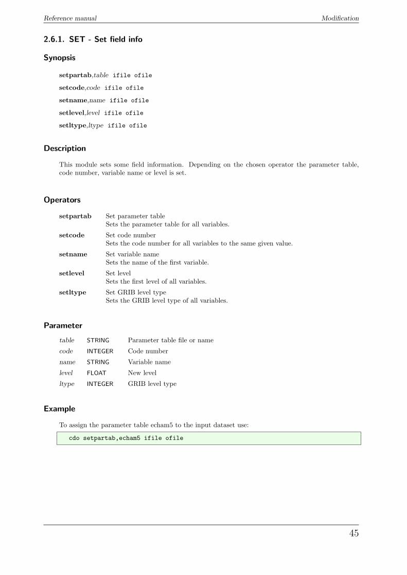
2.6.1. SET - Set field info
Synopsis
setpartab,table ifile ofile
setcode,code ifile ofile
setname,name ifile ofile
setlevel,level ifile ofile
setltype,ltype ifile ofile
Description
This module sets some field information. Depending on the chosen operator the parameter table,code number, variable name or level is set.
Operators
setpartab Set parameter tableSets the parameter table for all variables.
setcode Set code numberSets the code number for all variables to the same given value.
setname Set variable nameSets the name of the first variable.
setlevel Set levelSets the first level of all variables.
setltype Set GRIB level typeSets the GRIB level type of all variables.
Parameter
table STRING Parameter table file or name
code INTEGER Code number
name STRING Variable name
level FLOAT New level
ltype INTEGER GRIB level type
Example
To assign the parameter table echam5 to the input dataset use:
cdo setpartab,echam5 ifile ofile
45
Modification Reference manual
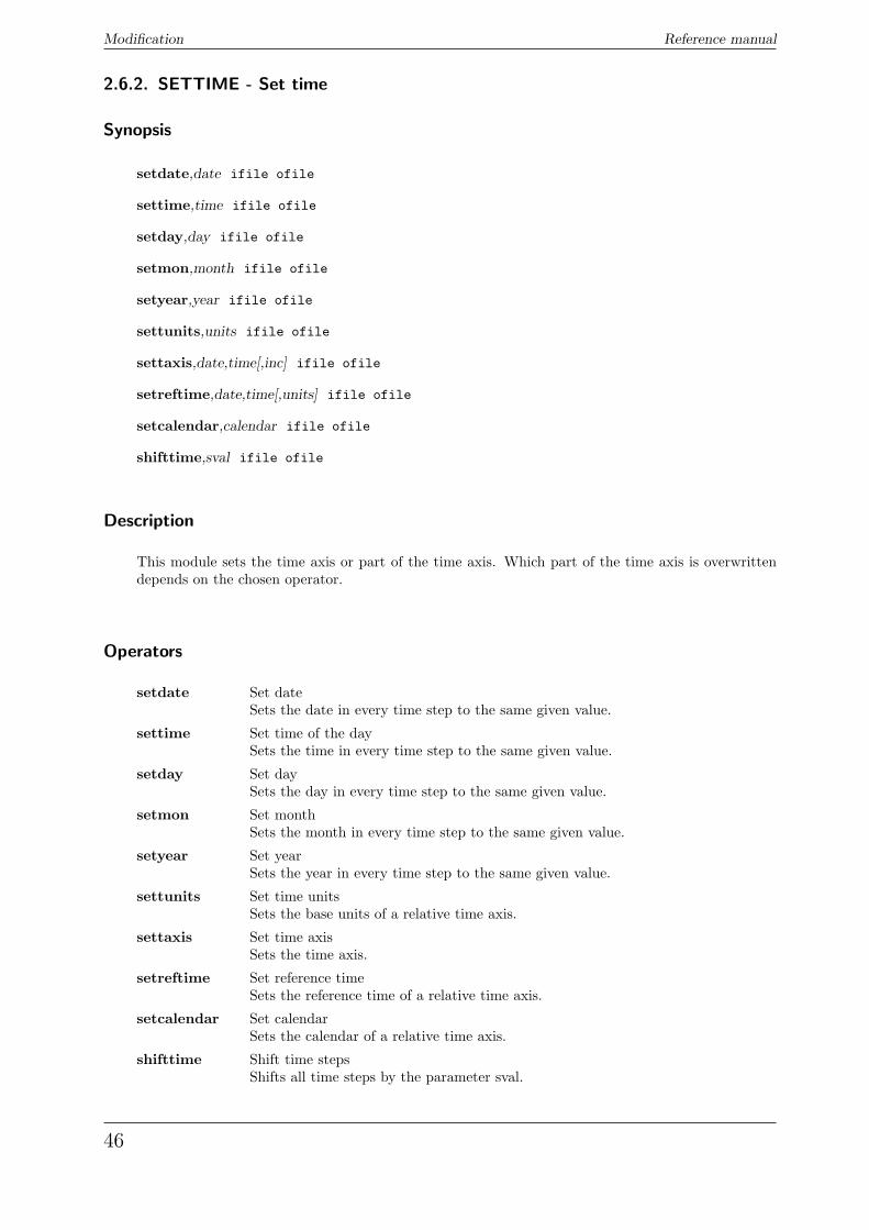
2.6.2. SETTIME - Set time
Synopsis
setdate,date ifile ofile
settime,time ifile ofile
setday,day ifile ofile
setmon,month ifile ofile
setyear,year ifile ofile
settunits,units ifile ofile
settaxis,date,time[,inc] ifile ofile
setreftime,date,time[,units] ifile ofile
setcalendar,calendar ifile ofile
shifttime,sval ifile ofile
Description
This module sets the time axis or part of the time axis. Which part of the time axis is overwrittendepends on the chosen operator.
Operators
setdate Set dateSets the date in every time step to the same given value.
settime Set time of the daySets the time in every time step to the same given value.
setday Set daySets the day in every time step to the same given value.
setmon Set monthSets the month in every time step to the same given value.
setyear Set yearSets the year in every time step to the same given value.
settunits Set time unitsSets the base units of a relative time axis.
settaxis Set time axisSets the time axis.
setreftime Set reference timeSets the reference time of a relative time axis.
setcalendar Set calendarSets the calendar of a relative time axis.
shifttime Shift time stepsShifts all time steps by the parameter sval.
46
Reference manual Modification
Parameter
day INTEGER Value of the new day
month INTEGER Value of the new month
year INTEGER Value of the new year
units STRING Base units of the time axis (seconds, minutes, hours, days, months, years)
date STRING Date (format YYYY-MM-DD)
time STRING Time (format hh:mm:ss)
inc STRING Optional increment (seconds, minutes, hours, days, months, years) [default:0hour]
calendar STRING Calendar (standard, proleptic, 360days, 365days, 366days)
sval STRING Shift value (e.g. -3hour)
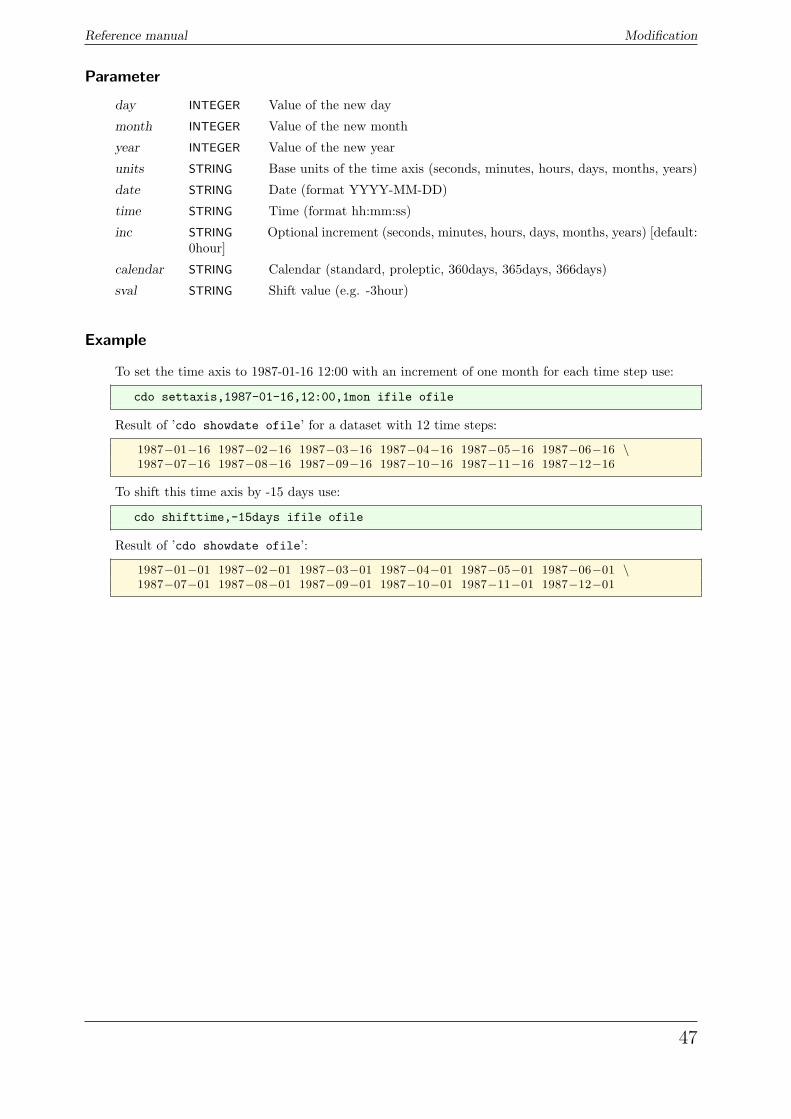
Example
To set the time axis to 1987-01-16 12:00 with an increment of one month for each time step use:
cdo settaxis,1987-01-16,12:00,1mon ifile ofile
Result of ’cdo showdate ofile’ for a dataset with 12 time steps:
1987−01−16 1987−02−16 1987−03−16 1987−04−16 1987−05−16 1987−06−16 \1987−07−16 1987−08−16 1987−09−16 1987−10−16 1987−11−16 1987−12−16
To shift this time axis by -15 days use:
cdo shifttime,-15days ifile ofile
Result of ’cdo showdate ofile’:
1987−01−01 1987−02−01 1987−03−01 1987−04−01 1987−05−01 1987−06−01 \1987−07−01 1987−08−01 1987−09−01 1987−10−01 1987−11−01 1987−12−01
47
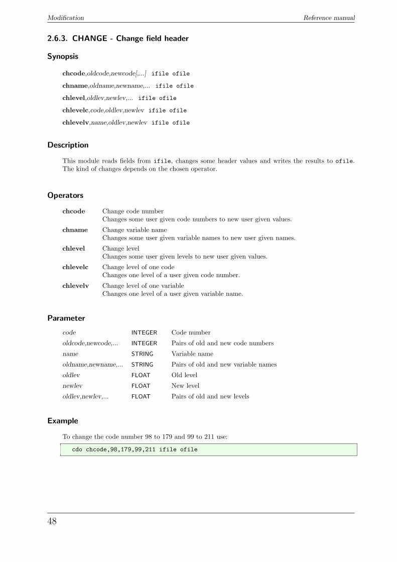
Modification Reference manual
2.6.3. CHANGE - Change field header
Synopsis
chcode,oldcode,newcode[,...] ifile ofile
chname,oldname,newname,... ifile ofile
chlevel,oldlev,newlev,... ifile ofile
chlevelc,code,oldlev,newlev ifile ofile
chlevelv,name,oldlev,newlev ifile ofile
Description
This module reads fields from ifile, changes some header values and writes the results to ofile.The kind of changes depends on the chosen operator.
Operators
chcode Change code numberChanges some user given code numbers to new user given values.
chname Change variable nameChanges some user given variable names to new user given names.
chlevel Change levelChanges some user given levels to new user given values.
chlevelc Change level of one codeChanges one level of a user given code number.
chlevelv Change level of one variableChanges one level of a user given variable name.
Parameter
code INTEGER Code number
oldcode,newcode,... INTEGER Pairs of old and new code numbers
name STRING Variable name
oldname,newname,... STRING Pairs of old and new variable names
oldlev FLOAT Old level
newlev FLOAT New level
oldlev,newlev,... FLOAT Pairs of old and new levels
Example
To change the code number 98 to 179 and 99 to 211 use:
cdo chcode,98,179,99,211 ifile ofile
48
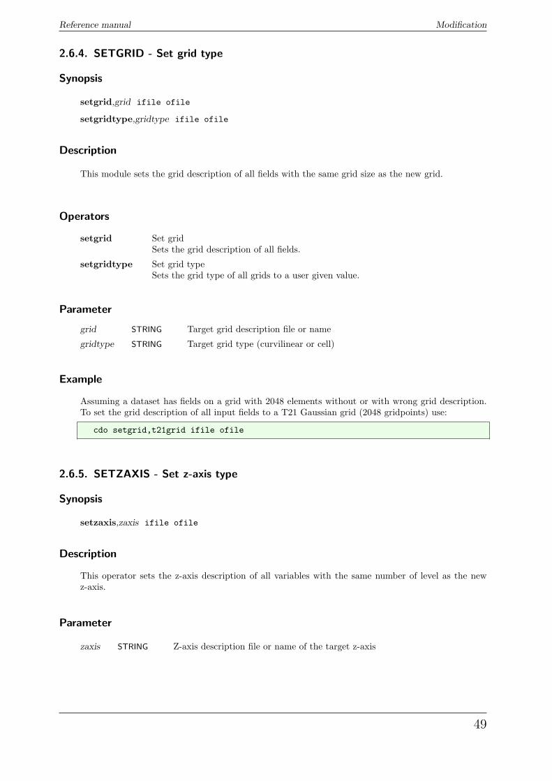
Reference manual Modification
2.6.4. SETGRID - Set grid type
Synopsis
setgrid,grid ifile ofile
setgridtype,gridtype ifile ofile
Description
This module sets the grid description of all fields with the same grid size as the new grid.
Operators
setgrid Set gridSets the grid description of all fields.
setgridtype Set grid typeSets the grid type of all grids to a user given value.
Parameter
grid STRING Target grid description file or name
gridtype STRING Target grid type (curvilinear or cell)
Example
Assuming a dataset has fields on a grid with 2048 elements without or with wrong grid description.To set the grid description of all input fields to a T21 Gaussian grid (2048 gridpoints) use:
cdo setgrid,t21grid ifile ofile
2.6.5. SETZAXIS - Set z-axis type
Synopsis
setzaxis,zaxis ifile ofile
Description
This operator sets the z-axis description of all variables with the same number of level as the newz-axis.
Parameter
zaxis STRING Z-axis description file or name of the target z-axis
49
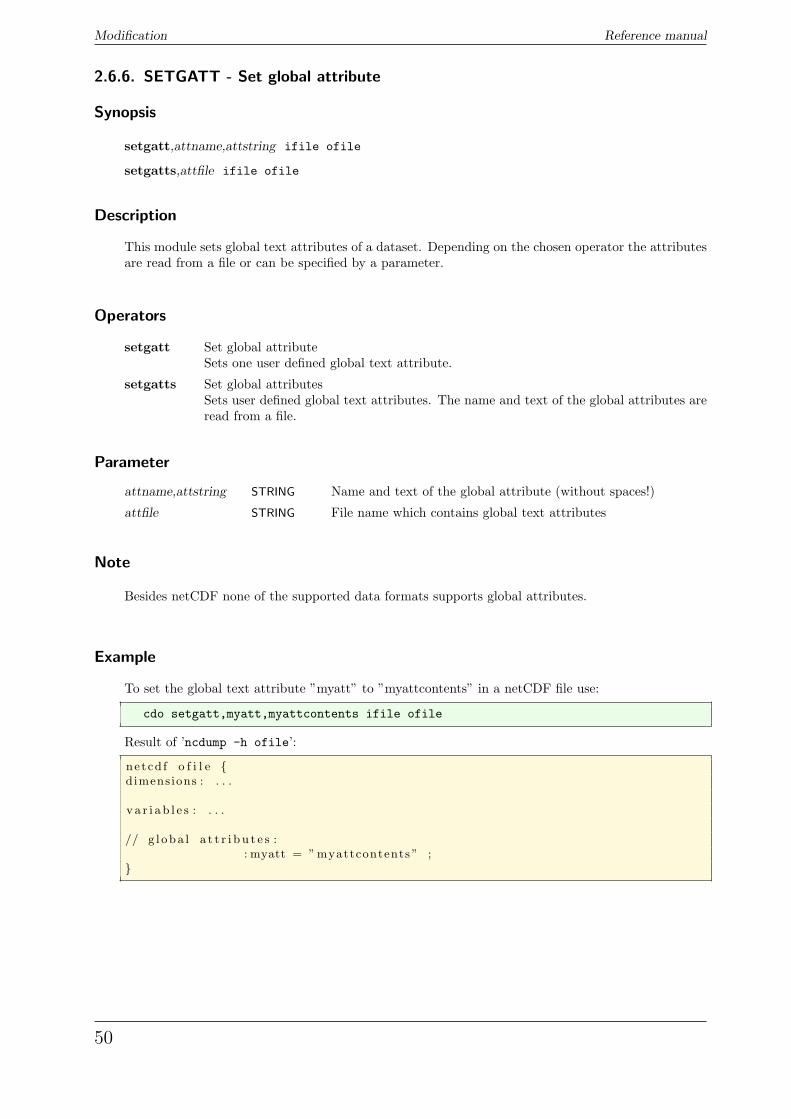
Modification Reference manual
2.6.6. SETGATT - Set global attribute
Synopsis
setgatt,attname,attstring ifile ofile
setgatts,attfile ifile ofile
Description
This module sets global text attributes of a dataset. Depending on the chosen operator the attributesare read from a file or can be specified by a parameter.
Operators
setgatt Set global attributeSets one user defined global text attribute.
setgatts Set global attributesSets user defined global text attributes. The name and text of the global attributes areread from a file.
Parameter
attname,attstring STRING Name and text of the global attribute (without spaces!)
attfile STRING File name which contains global text attributes
Note
Besides netCDF none of the supported data formats supports global attributes.
Example
To set the global text attribute ”myatt” to ”myattcontents” in a netCDF file use:
cdo setgatt,myatt,myattcontents ifile ofile
Result of ’ncdump -h ofile’:
netcd f o f i l e {dimensions : . . .
v a r i a b l e s : . . .
// g l oba l a t t r i b u t e s :: myatt = ”myattcontents ” ;
}
50
Reference manual Modification
2.6.7. INVERT - Invert latitudes
Synopsis
invertlat ifile ofile
Description
This operator inverts the latitudes of all fields with a regular lon/lat grid.
Example
To invert the latitudes of a 2D field from N->S to S->N use:
cdo invertlat ifile ofile
2.6.8. INVERTLEV - Invert levels
Synopsis
invertlev ifile ofile
Description
This operator inverts the levels of all non hybrid 3D variables.
51
Modification Reference manual
2.6.9. MASKREGION - Mask regions
Synopsis
maskregion,regions ifile ofile
Description
Masks different regions of fields with a regular lon/lat grid. The elements inside a region are un-touched, the elements outside are set to missing value. All input fields must have the same horizontalgrid. The user has to give ASCII formatted files with different regions. A region is defined by apolygon. Each line of a polygon description file contains the longitude and latitude of one point.Each polygon description file can contain one or more polygons separated by a line with the character&.
Parameter
regions STRING Comma separated list of ASCII formatted files with different regions
Example
To mask the region with the longitudes from 120E to 90W and latitudes from 20N to 20S on all inputfields use:
cdo maskregion,myregion ifile ofile
For this example the polygon description file myregion should contain the following four coordinates:
120 20120 −20270 −20270 20
52
Reference manual Modification
2.6.10. MASKBOX - Mask a box
Synopsis
masklonlatbox,lon1,lon2,lat1,lat2 ifile ofile
maskindexbox,idx1,idx2,idy1,idy2 ifile ofile
Description
Masks a box of the rectangular understood field. The elements inside the box are untouched, theelements outside are set to missing value. All input fields need to have the same horizontal grid. Usesellonlatbox or selindexbox if only the data inside the box are needed.
Operators
masklonlatbox Mask a longitude/latitude boxMasks a longitude/latitude box. The user has to give the longitudes and lati-tudes of the edges of the box.
maskindexbox Mask an index boxMasks an index box. The user has to give the indexes of the edges of the box.The index of the left edge can be greater then the one of the right edge.
Parameter
lon1 FLOAT Western longitude
lon2 FLOAT Eastern longitude
lat1 FLOAT Southern or northern latitude
lat2 FLOAT Northern or southern latitude
idx1 INTEGER Index of first longitude
idx2 INTEGER Index of last longitude
idy1 INTEGER Index of first latitude
idy2 INTEGER Index of last latitude
Example
To mask the region with the longitudes from 120E to 90W and latitudes from 20N to 20S on all inputfields use:
cdo masklonlatbox,120,-90,20,-20 ifile ofile
If the input dataset has fields on a T21 Gaussian grid, the same box can be masked with maskindexboxby:
cdo maskindexbox,23,48,13,20 ifile ofile
53
Modification Reference manual
2.6.11. SETBOX - Set a box to constant
Synopsis
setclonlatbox,c,lon1,lon2,lat1,lat2 ifile ofile
setcindexbox,c,idx1,idx2,idy1,idy2 ifile ofile
Description
Sets a box of the rectangular understood field to a constant value. The elements outside the box areuntouched, the elements inside are set to the given constant. All input fields need to have the samehorizontal grid.
Operators
setclonlatbox Set a longitude/latitude box to constantSets the values of a longitude/latitude box to a constant value. The user has togive the longitudes and latitudes of the edges of the box.
setcindexbox Set an index box to constantSets the values of an index box to a constant value. The user has to give theindexes of the edges of the box. The index of the left edge can be greater thanthe one of the right edge.
Parameter
c FLOAT Constant
lon1 FLOAT Western longitude
lon2 FLOAT Eastern longitude
lat1 FLOAT Southern or northern latitude
lat2 FLOAT Northern or southern latitude
idx1 INTEGER Index of first longitude
idx2 INTEGER Index of last longitude
idy1 INTEGER Index of first latitude
idy2 INTEGER Index of last latitude
Example
To set all values in the region with the longitudes from 120E to 90W and latitudes from 20N to 20Sto the constant value -1.23 use:
cdo setclonlatbox,-1.23,120,-90,20,-20 ifile ofile
If the input dataset has fields on a T21 Gaussian grid, the same box can be set with setcindexbox by:
cdo setcindexbox,-1.23,23,48,13,20 ifile ofile
54
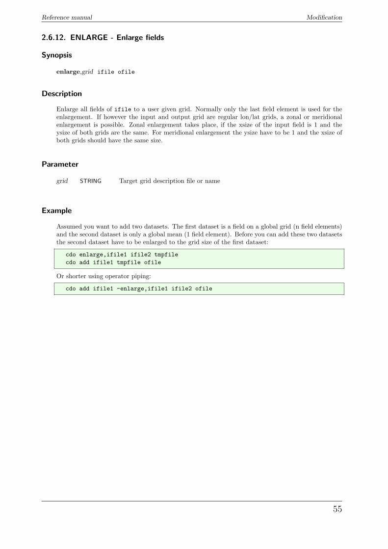
Reference manual Modification
2.6.12. ENLARGE - Enlarge fields
Synopsis
enlarge,grid ifile ofile
Description
Enlarge all fields of ifile to a user given grid. Normally only the last field element is used for theenlargement. If however the input and output grid are regular lon/lat grids, a zonal or meridionalenlargement is possible. Zonal enlargement takes place, if the xsize of the input field is 1 and theysize of both grids are the same. For meridional enlargement the ysize have to be 1 and the xsize ofboth grids should have the same size.
Parameter
grid STRING Target grid description file or name
Example
Assumed you want to add two datasets. The first dataset is a field on a global grid (n field elements)and the second dataset is only a global mean (1 field element). Before you can add these two datasetsthe second dataset have to be enlarged to the grid size of the first dataset:
cdo enlarge,ifile1 ifile2 tmpfilecdo add ifile1 tmpfile ofile
Or shorter using operator piping:
cdo add ifile1 -enlarge,ifile1 ifile2 ofile
55
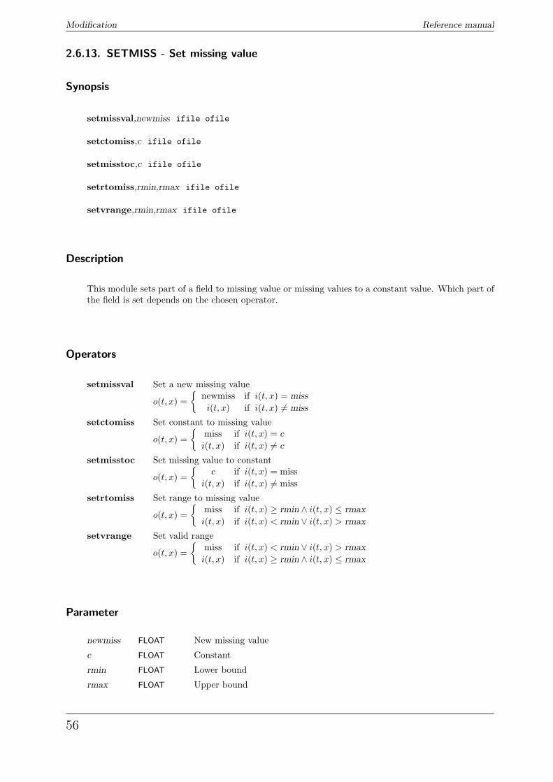
Modification Reference manual
2.6.13. SETMISS - Set missing value
Synopsis
setmissval,newmiss ifile ofile
setctomiss,c ifile ofile
setmisstoc,c ifile ofile
setrtomiss,rmin,rmax ifile ofile
setvrange,rmin,rmax ifile ofile
Description
This module sets part of a field to missing value or missing values to a constant value. Which part ofthe field is set depends on the chosen operator.
Operators
setmissval Set a new missing value
o(t, x) ={
newmiss if i(t, x) = miss
i(t, x) if i(t, x) 6= miss
setctomiss Set constant to missing value
o(t, x) ={
miss if i(t, x) = c
i(t, x) if i(t, x) 6= c
setmisstoc Set missing value to constant
o(t, x) ={
c if i(t, x) = missi(t, x) if i(t, x) 6= miss
setrtomiss Set range to missing value
o(t, x) ={
miss if i(t, x) ≥ rmin ∧ i(t, x) ≤ rmax
i(t, x) if i(t, x) < rmin ∨ i(t, x) > rmax
setvrange Set valid range
o(t, x) ={
miss if i(t, x) < rmin ∨ i(t, x) > rmax
i(t, x) if i(t, x) ≥ rmin ∧ i(t, x) ≤ rmax
Parameter
newmiss FLOAT New missing value
c FLOAT Constant
rmin FLOAT Lower bound
rmax FLOAT Upper bound
56
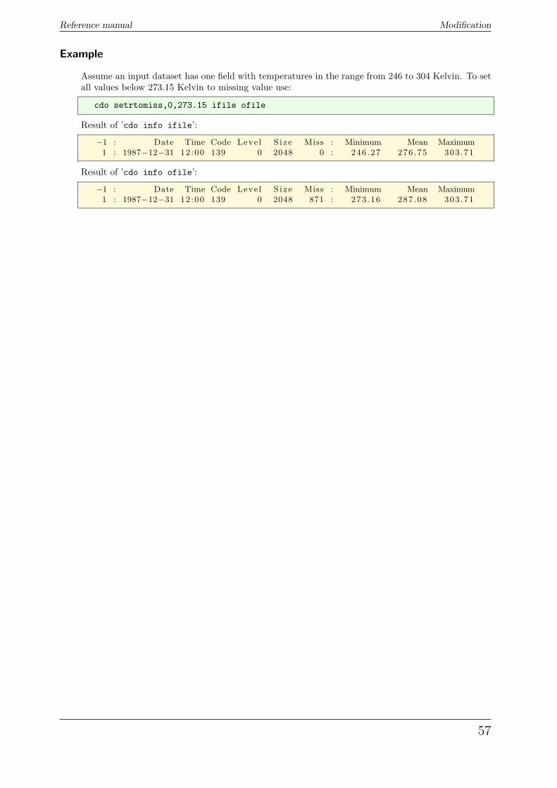
Reference manual Modification
Example
Assume an input dataset has one field with temperatures in the range from 246 to 304 Kelvin. To setall values below 273.15 Kelvin to missing value use:
cdo setrtomiss,0,273.15 ifile ofile
Result of ’cdo info ifile’:
−1 : Date Time Code Leve l S i z e Miss : Minimum Mean Maximum1 : 1987−12−31 12 :00 139 0 2048 0 : 246 .27 276 .75 303 .71
Result of ’cdo info ofile’:
−1 : Date Time Code Leve l S i z e Miss : Minimum Mean Maximum1 : 1987−12−31 12 :00 139 0 2048 871 : 273 .16 287 .08 303 .71
57
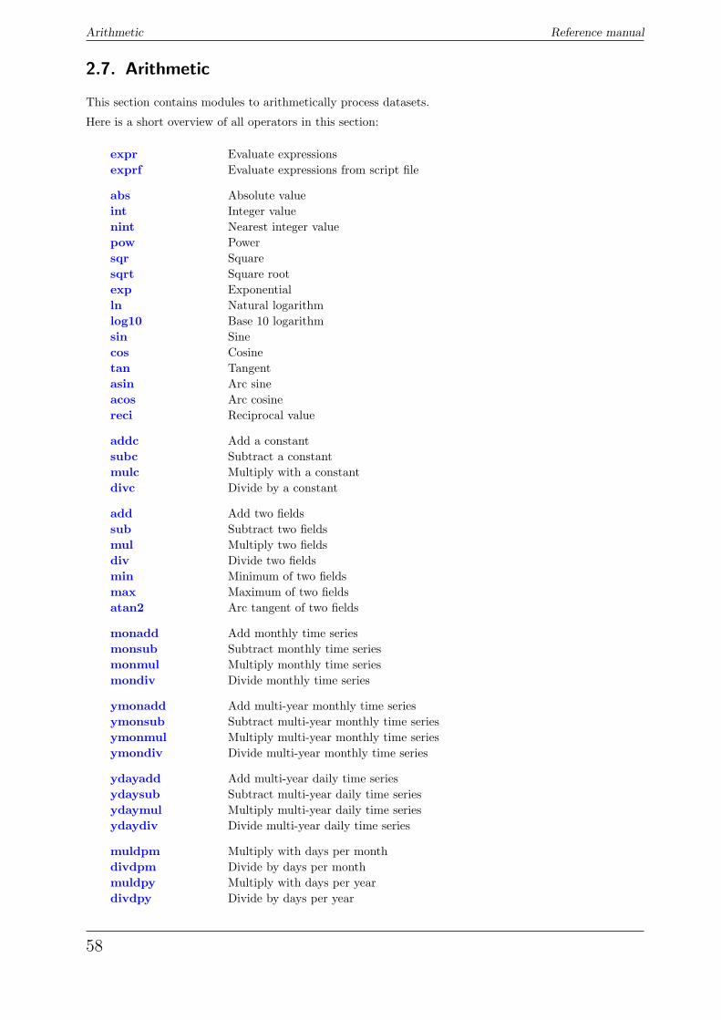
Arithmetic Reference manual
2.7. Arithmetic
This section contains modules to arithmetically process datasets.
Here is a short overview of all operators in this section:
expr Evaluate expressionsexprf Evaluate expressions from script file
abs Absolute valueint Integer valuenint Nearest integer valuepow Powersqr Squaresqrt Square rootexp Exponentialln Natural logarithmlog10 Base 10 logarithmsin Sinecos Cosinetan Tangentasin Arc sineacos Arc cosinereci Reciprocal value
addc Add a constantsubc Subtract a constantmulc Multiply with a constantdivc Divide by a constant
add Add two fieldssub Subtract two fieldsmul Multiply two fieldsdiv Divide two fieldsmin Minimum of two fieldsmax Maximum of two fieldsatan2 Arc tangent of two fields
monadd Add monthly time seriesmonsub Subtract monthly time seriesmonmul Multiply monthly time seriesmondiv Divide monthly time series
ymonadd Add multi-year monthly time seriesymonsub Subtract multi-year monthly time seriesymonmul Multiply multi-year monthly time seriesymondiv Divide multi-year monthly time series
ydayadd Add multi-year daily time seriesydaysub Subtract multi-year daily time seriesydaymul Multiply multi-year daily time seriesydaydiv Divide multi-year daily time series
muldpm Multiply with days per monthdivdpm Divide by days per monthmuldpy Multiply with days per yeardivdpy Divide by days per year
58
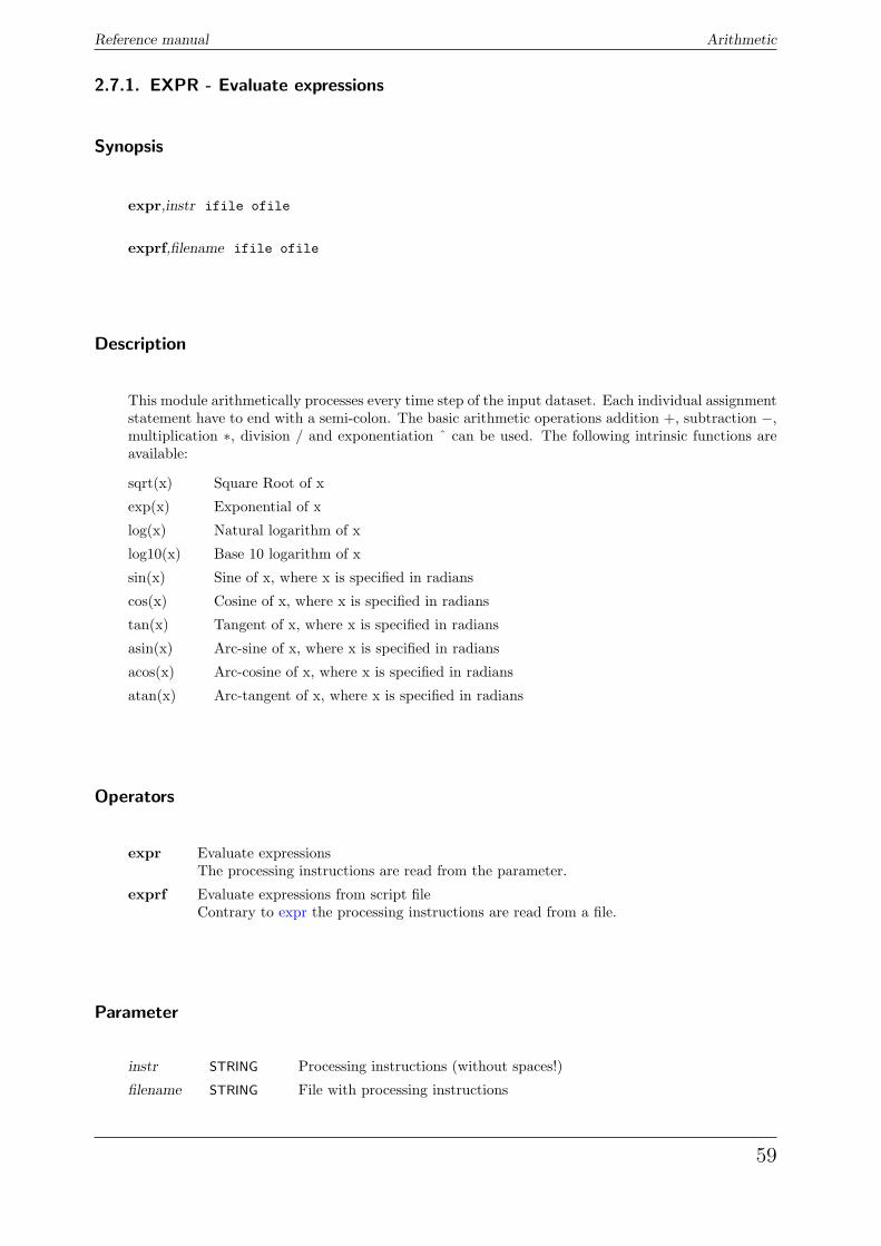
Reference manual Arithmetic
2.7.1. EXPR - Evaluate expressions
Synopsis
expr,instr ifile ofile
exprf,filename ifile ofile
Description
This module arithmetically processes every time step of the input dataset. Each individual assignmentstatement have to end with a semi-colon. The basic arithmetic operations addition +, subtraction −,multiplication ∗, division / and exponentiation ˆ can be used. The following intrinsic functions areavailable:
sqrt(x) Square Root of x
exp(x) Exponential of x
log(x) Natural logarithm of x
log10(x) Base 10 logarithm of x
sin(x) Sine of x, where x is specified in radians
cos(x) Cosine of x, where x is specified in radians
tan(x) Tangent of x, where x is specified in radians
asin(x) Arc-sine of x, where x is specified in radians
acos(x) Arc-cosine of x, where x is specified in radians
atan(x) Arc-tangent of x, where x is specified in radians
Operators
expr Evaluate expressionsThe processing instructions are read from the parameter.
exprf Evaluate expressions from script fileContrary to expr the processing instructions are read from a file.
Parameter
instr STRING Processing instructions (without spaces!)
filename STRING File with processing instructions
59
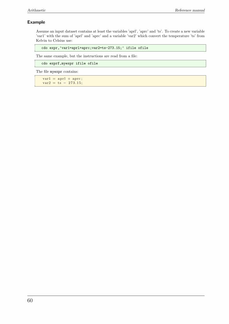
Arithmetic Reference manual
Example
Assume an input dataset contains at least the variables ’aprl’, ’aprc’ and ’ts’. To create a new variable’var1’ with the sum of ’aprl’ and ’aprc’ and a variable ’var2’ which convert the temperature ’ts’ fromKelvin to Celsius use:
cdo expr,’var1=aprl+aprc;var2=ts-273.15;’ ifile ofile
The same example, but the instructions are read from a file:
cdo exprf,myexpr ifile ofile
The file myexpr contains:
var1 = apr l + aprc ;var2 = t s − 273 . 1 5 ;
60
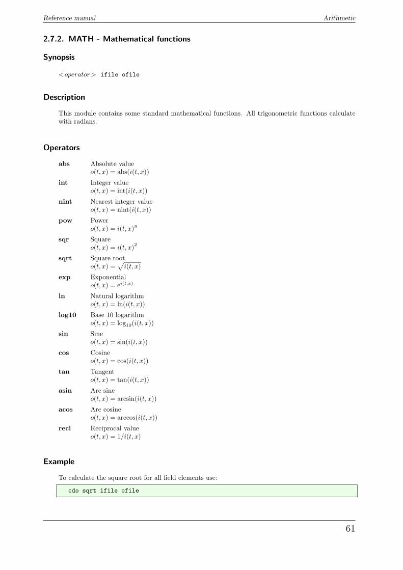
Reference manual Arithmetic
2.7.2. MATH - Mathematical functions
Synopsis
<operator> ifile ofile
Description
This module contains some standard mathematical functions. All trigonometric functions calculatewith radians.
Operators
abs Absolute valueo(t, x) = abs(i(t, x))
int Integer valueo(t, x) = int(i(t, x))
nint Nearest integer valueo(t, x) = nint(i(t, x))
pow Powero(t, x) = i(t, x)y
sqr Squareo(t, x) = i(t, x)2
sqrt Square rooto(t, x) =
√i(t, x)
exp Exponentialo(t, x) = ei(t,x)
ln Natural logarithmo(t, x) = ln(i(t, x))
log10 Base 10 logarithmo(t, x) = log10(i(t, x))
sin Sineo(t, x) = sin(i(t, x))
cos Cosineo(t, x) = cos(i(t, x))
tan Tangento(t, x) = tan(i(t, x))
asin Arc sineo(t, x) = arcsin(i(t, x))
acos Arc cosineo(t, x) = arccos(i(t, x))
reci Reciprocal valueo(t, x) = 1/i(t, x)
Example
To calculate the square root for all field elements use:
cdo sqrt ifile ofile
61
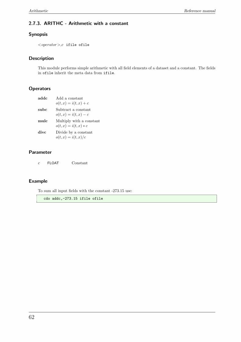
Arithmetic Reference manual
2.7.3. ARITHC - Arithmetic with a constant
Synopsis
<operator>,c ifile ofile
Description
This module performs simple arithmetic with all field elements of a dataset and a constant. The fieldsin ofile inherit the meta data from ifile.
Operators
addc Add a constanto(t, x) = i(t, x) + c
subc Subtract a constanto(t, x) = i(t, x)− c
mulc Multiply with a constanto(t, x) = i(t, x) ∗ c
divc Divide by a constanto(t, x) = i(t, x)/c
Parameter
c FLOAT Constant
Example
To sum all input fields with the constant -273.15 use:
cdo addc,-273.15 ifile ofile
62
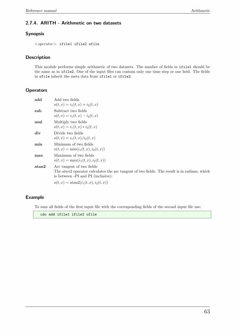
Reference manual Arithmetic
2.7.4. ARITH - Arithmetic on two datasets
Synopsis
<operator> ifile1 ifile2 ofile
Description
This module performs simple arithmetic of two datasets. The number of fields in ifile1 should bethe same as in ifile2. One of the input files can contain only one time step or one field. The fieldsin ofile inherit the meta data from ifile1 or ifile2.
Operators
add Add two fieldso(t, x) = i1(t, x) + i2(t, x)
sub Subtract two fieldso(t, x) = i1(t, x)− i2(t, x)
mul Multiply two fieldso(t, x) = i1(t, x) ∗ i2(t, x)
div Divide two fieldso(t, x) = i1(t, x)/i2(t, x)
min Minimum of two fieldso(t, x) = min(i1(t, x), i2(t, x))
max Maximum of two fieldso(t, x) = max(i1(t, x), i2(t, x))
atan2 Arc tangent of two fieldsThe atan2 operator calculates the arc tangent of two fields. The result is in radians, whichis between -PI and PI (inclusive).
o(t, x) = atan2(i1(t, x), i2(t, x))
Example
To sum all fields of the first input file with the corresponding fields of the second input file use:
cdo add ifile1 ifile2 ofile
63
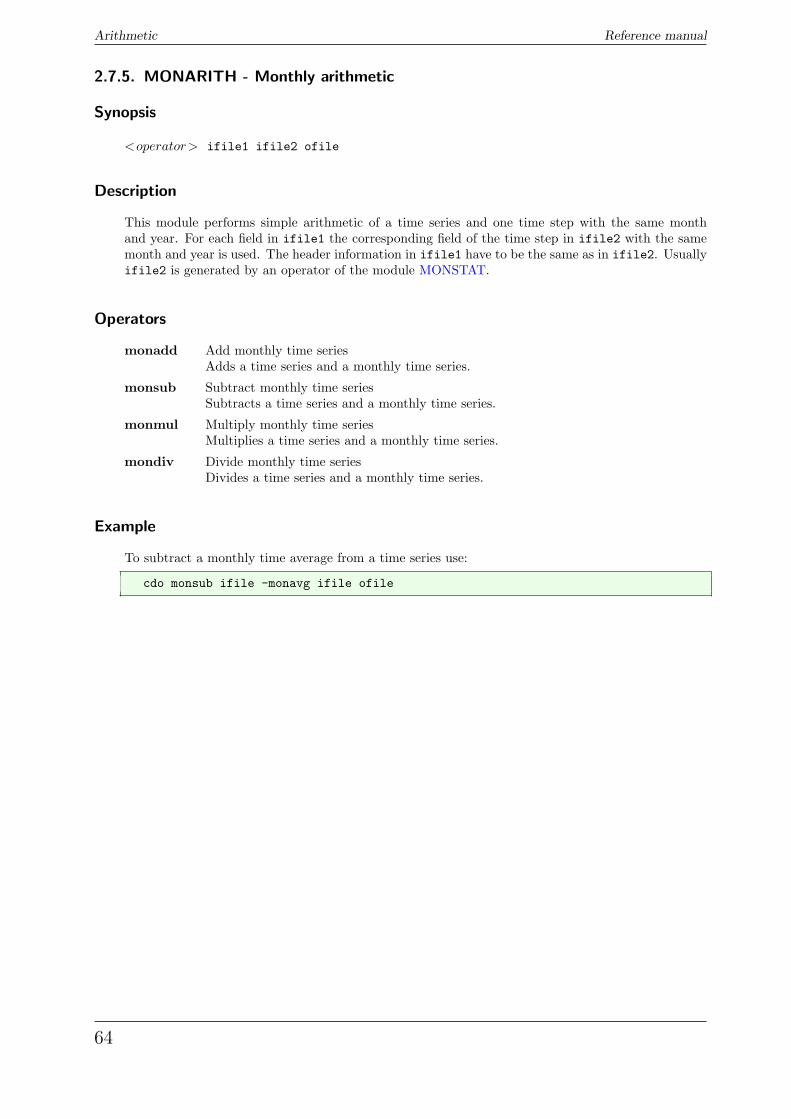
Arithmetic Reference manual
2.7.5. MONARITH - Monthly arithmetic
Synopsis
<operator> ifile1 ifile2 ofile
Description
This module performs simple arithmetic of a time series and one time step with the same monthand year. For each field in ifile1 the corresponding field of the time step in ifile2 with the samemonth and year is used. The header information in ifile1 have to be the same as in ifile2. Usuallyifile2 is generated by an operator of the module MONSTAT.
Operators
monadd Add monthly time seriesAdds a time series and a monthly time series.
monsub Subtract monthly time seriesSubtracts a time series and a monthly time series.
monmul Multiply monthly time seriesMultiplies a time series and a monthly time series.
mondiv Divide monthly time seriesDivides a time series and a monthly time series.
Example
To subtract a monthly time average from a time series use:
cdo monsub ifile -monavg ifile ofile
64
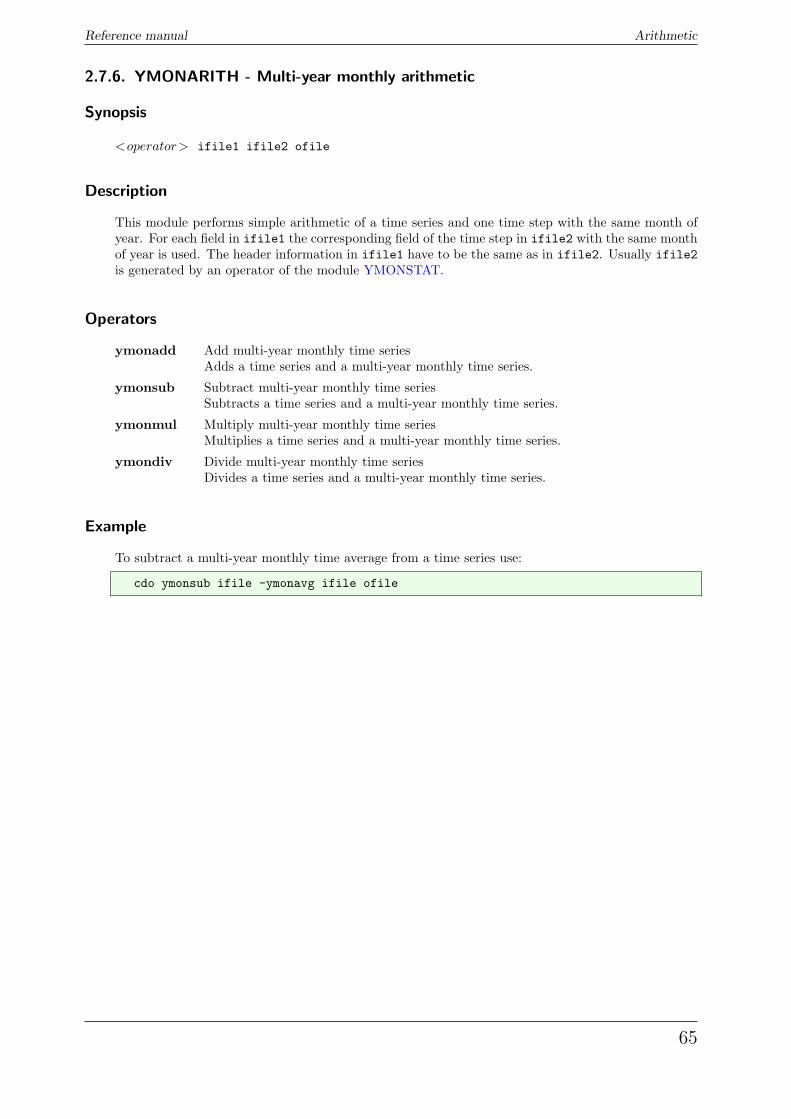
Reference manual Arithmetic
2.7.6. YMONARITH - Multi-year monthly arithmetic
Synopsis
<operator> ifile1 ifile2 ofile
Description
This module performs simple arithmetic of a time series and one time step with the same month ofyear. For each field in ifile1 the corresponding field of the time step in ifile2 with the same monthof year is used. The header information in ifile1 have to be the same as in ifile2. Usually ifile2is generated by an operator of the module YMONSTAT.
Operators
ymonadd Add multi-year monthly time seriesAdds a time series and a multi-year monthly time series.
ymonsub Subtract multi-year monthly time seriesSubtracts a time series and a multi-year monthly time series.
ymonmul Multiply multi-year monthly time seriesMultiplies a time series and a multi-year monthly time series.
ymondiv Divide multi-year monthly time seriesDivides a time series and a multi-year monthly time series.
Example
To subtract a multi-year monthly time average from a time series use:
cdo ymonsub ifile -ymonavg ifile ofile
65
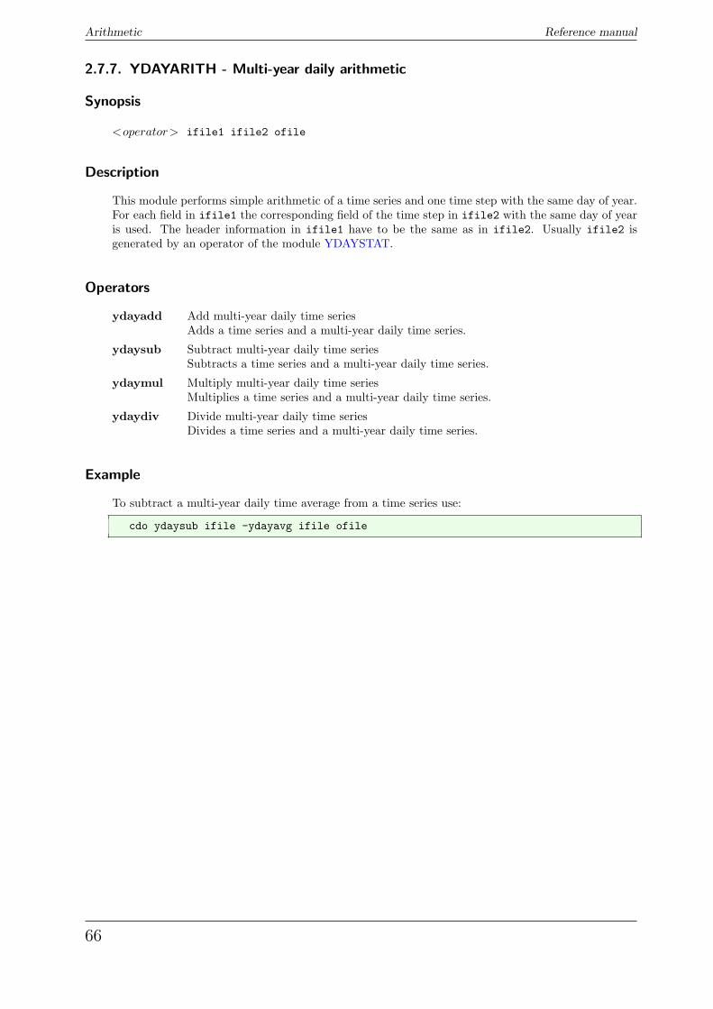
Arithmetic Reference manual
2.7.7. YDAYARITH - Multi-year daily arithmetic
Synopsis
<operator> ifile1 ifile2 ofile
Description
This module performs simple arithmetic of a time series and one time step with the same day of year.For each field in ifile1 the corresponding field of the time step in ifile2 with the same day of yearis used. The header information in ifile1 have to be the same as in ifile2. Usually ifile2 isgenerated by an operator of the module YDAYSTAT.
Operators
ydayadd Add multi-year daily time seriesAdds a time series and a multi-year daily time series.
ydaysub Subtract multi-year daily time seriesSubtracts a time series and a multi-year daily time series.
ydaymul Multiply multi-year daily time seriesMultiplies a time series and a multi-year daily time series.
ydaydiv Divide multi-year daily time seriesDivides a time series and a multi-year daily time series.
Example
To subtract a multi-year daily time average from a time series use:
cdo ydaysub ifile -ydayavg ifile ofile
66
Reference manual Arithmetic
2.7.8. ARITHDAYS - Arithmetic with days
Synopsis
<operator> ifile ofile
Description
This module multiplies or divides each time step of a dataset with the corresponding days per monthor days per year. The result of these functions depends on the used calendar of the input data.
Operators
muldpm Multiply with days per montho(t, x) = i(t, x) ∗ days per month
divdpm Divide by days per montho(t, x) = i(t, x)/days per month
muldpy Multiply with days per yearo(t, x) = i(t, x) ∗ days per year
divdpy Divide by days per yearo(t, x) = i(t, x)/days per year
Example
Assume an input dataset is a monthly mean time series. To compute the yearly mean from the correctweighted monthly mean use:
cdo muldpm ifile tmpfile1cdo yearsum tmpfile1 tmpfile2cdo divdpy tmpfile2 ofile
Or all in one command line:
cdo divdpy -yearsum -muldpm ifile ofile
67
Statistical values Reference manual
2.8. Statistical values
This section contains modules to compute statistical values of datasets. In this program there is thedifferent notion of ”mean” and ”average” to distinguish two different kinds of treatment of missing values.While computing the mean, only the not missing values are considered to belong to the sample with theside effect of a probably reduced sample size. Computing the average is just adding the sample membersand divide the result by the sample size. For example, the mean of 1, 2, miss and 3 is (1+2+3)/3 = 2,whereas the average is (1+2+miss+3)/4 = miss/4 = miss. If there are no missing values in the sample,the average and the mean are identical.In this section the abbreviations as in the following table are used:
sumn∑
i=1
xi
mean resp. avg n−1n∑
i=1
xi
mean resp. avgweighted by{wi, i = 1, ..., n}
n∑j=1
wj
−1n∑
i=1
wi xi
Variancevar
n−1n∑
i=1
(xi − x)2
var weighted by{wi, i = 1, ..., n}
n∑j=1
wj
−1n∑
i=1
wi
xi −
n∑j=1
wj
−1n∑
j=1
wj xj
2
Standard deviationstd
√√√√n−1
n∑i=1
(xi − x)2
std weighted by{wi, i = 1, ..., n}
√√√√√√ n∑
j=1
wj
−1n∑
i=1
wi
xi −
n∑j=1
wj
−1n∑
j=1
wj xj
2
Cumulative RankedProbability Scorecrps
∫ ∞
−∞[H(x1)− cdf({x2 . . . xn})|r]2 dr
with cdf(X)|r being the cumulative distribution function of {xi, i = 2 . . . n} at r
and H(x) the Heavyside function jumping at x.
Here is a short overview of all operators in this section:
consecsum Consecutive Sumconsects Consecutive Timesteps
68
Reference manual Statistical values
ensmin Ensemble minimumensmax Ensemble maximumenssum Ensemble sumensmean Ensemble meanensavg Ensemble averageensvar Ensemble varianceensstd Ensemble standard deviationenspctl Ensemble percentiles
ensbrs Brier scoreenscrps Cumulative Ranked Probability scoreensrkhistspace Ranked Histogram averaged over timeensrkhisttime Ranked Histogram averaged over spaceensroc Ensemble Receiver Operating characteristics
fldmin Field minimumfldmax Field maximumfldsum Field sumfldmean Field meanfldavg Field averagefldvar Field variancefldstd Field standard deviationfldpctl Field percentiles
zonmin Zonal minimumzonmax Zonal maximumzonsum Zonal sumzonmean Zonal meanzonavg Zonal averagezonvar Zonal variancezonstd Zonal standard deviationzonpctl Zonal percentiles
mermin Meridional minimummermax Meridional maximummersum Meridional summermean Meridional meanmeravg Meridional averagemervar Meridional variancemerstd Meridional standard deviationmerpctl Meridional percentiles
gridboxmin Gridbox minimumgridboxmax Gridbox maximumgridboxsum Gridbox sumgridboxmean Gridbox meangridboxavg Gridbox averagegridboxvar Gridbox variancegridboxstd Gridbox standard deviation
69
Statistical values Reference manual
vertmin Vertical minimumvertmax Vertical maximumvertsum Vertical sumvertmean Vertical meanvertavg Vertical averagevertvar Vertical variancevertstd Vertical standard deviation
timselmin Time range minimumtimselmax Time range maximumtimselsum Time range sumtimselmean Time range meantimselavg Time range averagetimselvar Time range variancetimselstd Time range standard deviation
timselpctl Time range percentiles
runmin Running minimumrunmax Running maximumrunsum Running sumrunmean Running meanrunavg Running averagerunvar Running variancerunstd Running standard deviation
runpctl Running percentiles
timmin Time minimumtimmax Time maximumtimsum Time sumtimmean Time meantimavg Time averagetimvar Time variancetimstd Time standard deviation
timpctl Time percentiles
hourmin Hourly minimumhourmax Hourly maximumhoursum Hourly sumhourmean Hourly meanhouravg Hourly averagehourvar Hourly variancehourstd Hourly standard deviation
hourpctl Hourly percentiles
daymin Daily minimumdaymax Daily maximumdaysum Daily sumdaymean Daily meandayavg Daily averagedayvar Daily variancedaystd Daily standard deviation
70
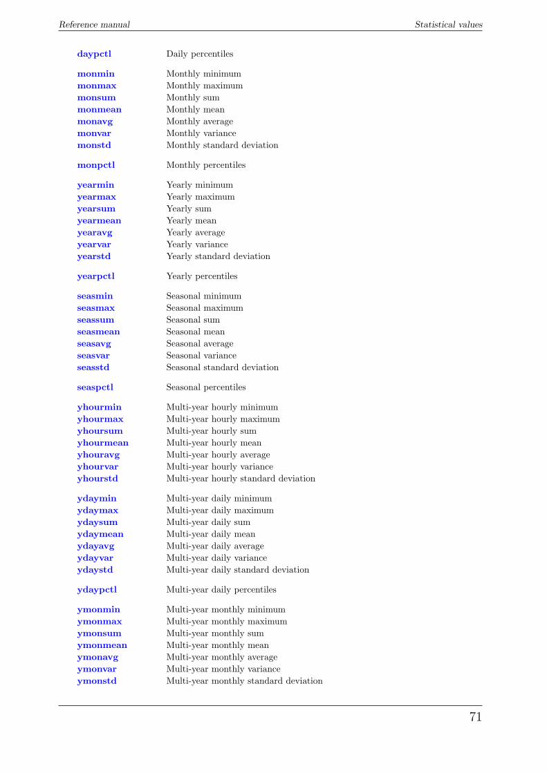
Reference manual Statistical values
daypctl Daily percentiles
monmin Monthly minimummonmax Monthly maximummonsum Monthly summonmean Monthly meanmonavg Monthly averagemonvar Monthly variancemonstd Monthly standard deviation
monpctl Monthly percentiles
yearmin Yearly minimumyearmax Yearly maximumyearsum Yearly sumyearmean Yearly meanyearavg Yearly averageyearvar Yearly varianceyearstd Yearly standard deviation
yearpctl Yearly percentiles
seasmin Seasonal minimumseasmax Seasonal maximumseassum Seasonal sumseasmean Seasonal meanseasavg Seasonal averageseasvar Seasonal varianceseasstd Seasonal standard deviation
seaspctl Seasonal percentiles
yhourmin Multi-year hourly minimumyhourmax Multi-year hourly maximumyhoursum Multi-year hourly sumyhourmean Multi-year hourly meanyhouravg Multi-year hourly averageyhourvar Multi-year hourly varianceyhourstd Multi-year hourly standard deviation
ydaymin Multi-year daily minimumydaymax Multi-year daily maximumydaysum Multi-year daily sumydaymean Multi-year daily meanydayavg Multi-year daily averageydayvar Multi-year daily varianceydaystd Multi-year daily standard deviation
ydaypctl Multi-year daily percentiles
ymonmin Multi-year monthly minimumymonmax Multi-year monthly maximumymonsum Multi-year monthly sumymonmean Multi-year monthly meanymonavg Multi-year monthly averageymonvar Multi-year monthly varianceymonstd Multi-year monthly standard deviation
71
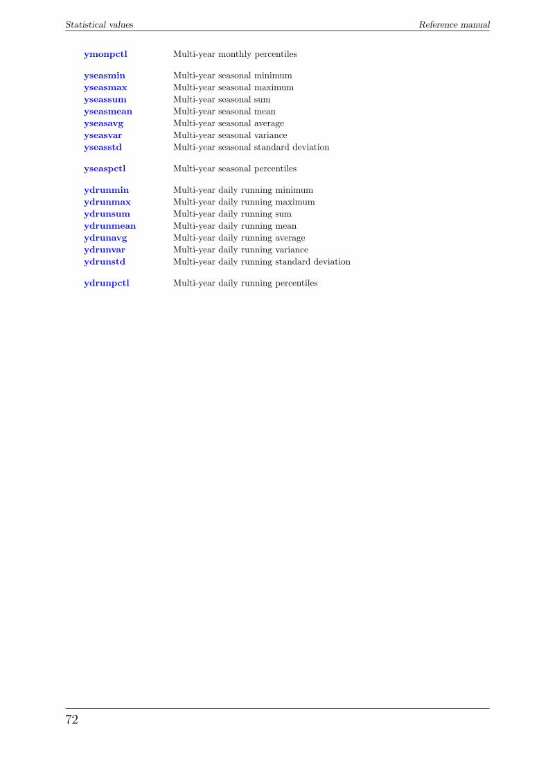
Statistical values Reference manual
ymonpctl Multi-year monthly percentiles
yseasmin Multi-year seasonal minimumyseasmax Multi-year seasonal maximumyseassum Multi-year seasonal sumyseasmean Multi-year seasonal meanyseasavg Multi-year seasonal averageyseasvar Multi-year seasonal varianceyseasstd Multi-year seasonal standard deviation
yseaspctl Multi-year seasonal percentiles
ydrunmin Multi-year daily running minimumydrunmax Multi-year daily running maximumydrunsum Multi-year daily running sumydrunmean Multi-year daily running meanydrunavg Multi-year daily running averageydrunvar Multi-year daily running varianceydrunstd Multi-year daily running standard deviation
ydrunpctl Multi-year daily running percentiles
72
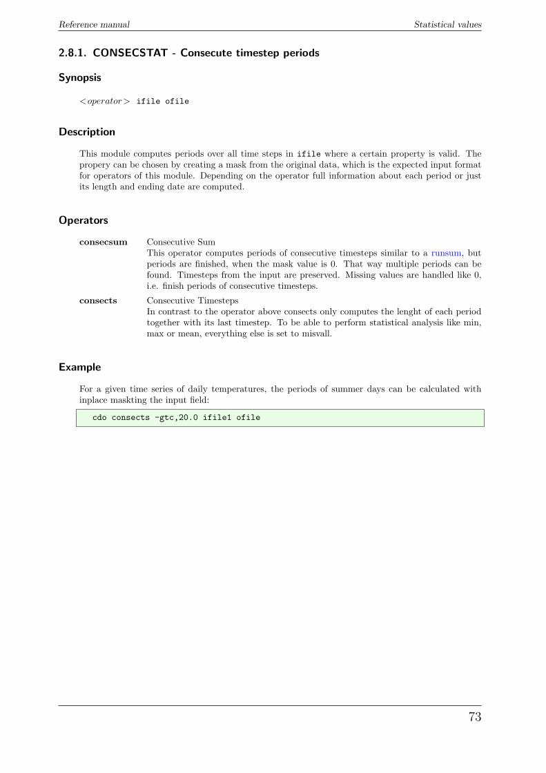
Reference manual Statistical values
2.8.1. CONSECSTAT - Consecute timestep periods
Synopsis
<operator> ifile ofile
Description
This module computes periods over all time steps in ifile where a certain property is valid. Thepropery can be chosen by creating a mask from the original data, which is the expected input formatfor operators of this module. Depending on the operator full information about each period or justits length and ending date are computed.
Operators
consecsum Consecutive SumThis operator computes periods of consecutive timesteps similar to a runsum, butperiods are finished, when the mask value is 0. That way multiple periods can befound. Timesteps from the input are preserved. Missing values are handled like 0,i.e. finish periods of consecutive timesteps.
consects Consecutive TimestepsIn contrast to the operator above consects only computes the lenght of each periodtogether with its last timestep. To be able to perform statistical analysis like min,max or mean, everything else is set to misvall.
Example
For a given time series of daily temperatures, the periods of summer days can be calculated withinplace maskting the input field:
cdo consects -gtc,20.0 ifile1 ofile
73
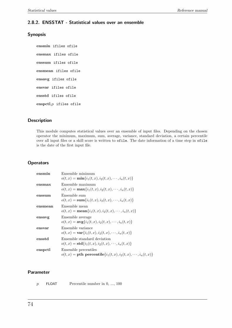
Statistical values Reference manual
2.8.2. ENSSTAT - Statistical values over an ensemble
Synopsis
ensmin ifiles ofile
ensmax ifiles ofile
enssum ifiles ofile
ensmean ifiles ofile
ensavg ifiles ofile
ensvar ifiles ofile
ensstd ifiles ofile
enspctl,p ifiles ofile
Description
This module computes statistical values over an ensemble of input files. Depending on the chosenoperator the minimum, maximum, sum, average, variance, standard deviation, a certain percentileover all input files or a skill score is written to ofile. The date information of a time step in ofileis the date of the first input file.
Operators
ensmin Ensemble minimumo(t, x) = min{i1(t, x), i2(t, x), · · · , in(t, x)}
ensmax Ensemble maximumo(t, x) = max{i1(t, x), i2(t, x), · · · , in(t, x)}
enssum Ensemble sumo(t, x) = sum{i1(t, x), i2(t, x), · · · , in(t, x)}
ensmean Ensemble meano(t, x) = mean{i1(t, x), i2(t, x), · · · , in(t, x)}
ensavg Ensemble averageo(t, x) = avg{i1(t, x), i2(t, x), · · · , in(t, x)}
ensvar Ensemble varianceo(t, x) = var{i1(t, x), i2(t, x), · · · , in(t, x)}
ensstd Ensemble standard deviationo(t, x) = std{i1(t, x), i2(t, x), · · · , in(t, x)}
enspctl Ensemble percentileso(t, x) = pth percentile{i1(t, x), i2(t, x), · · · , in(t, x)}
Parameter
p FLOAT Percentile number in 0, ..., 100
74
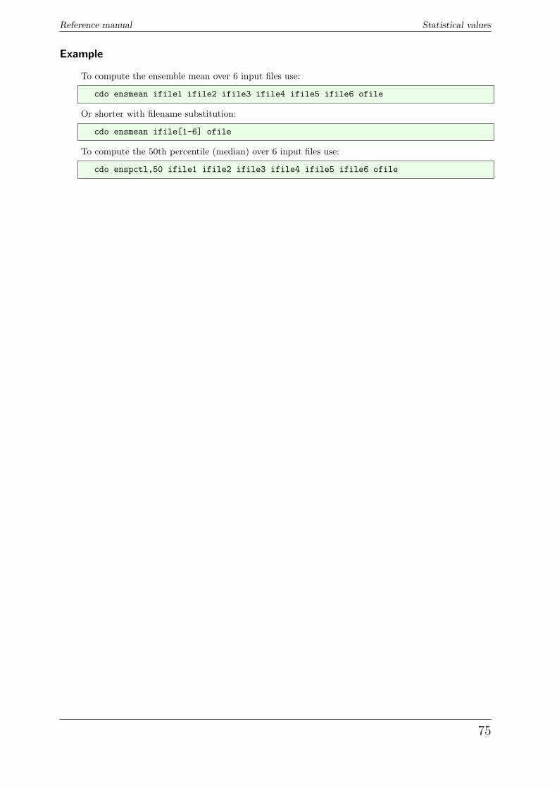
Reference manual Statistical values
Example
To compute the ensemble mean over 6 input files use:
cdo ensmean ifile1 ifile2 ifile3 ifile4 ifile5 ifile6 ofile
Or shorter with filename substitution:
cdo ensmean ifile[1-6] ofile
To compute the 50th percentile (median) over 6 input files use:
cdo enspctl,50 ifile1 ifile2 ifile3 ifile4 ifile5 ifile6 ofile
75
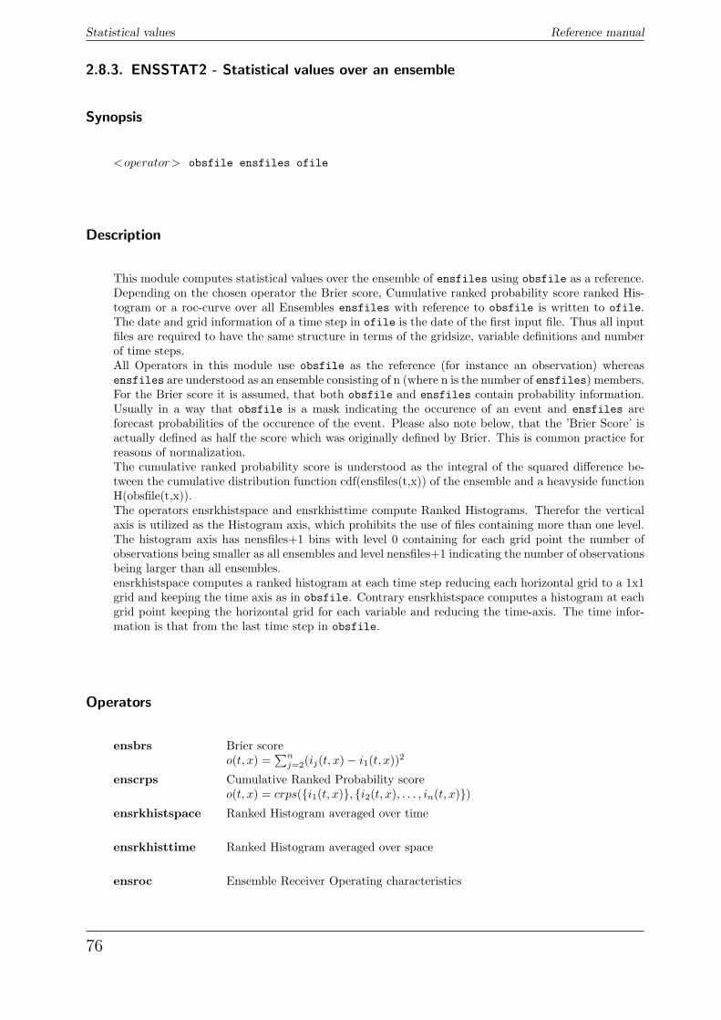
Statistical values Reference manual
2.8.3. ENSSTAT2 - Statistical values over an ensemble
Synopsis
<operator> obsfile ensfiles ofile
Description
This module computes statistical values over the ensemble of ensfiles using obsfile as a reference.Depending on the chosen operator the Brier score, Cumulative ranked probability score ranked His-togram or a roc-curve over all Ensembles ensfiles with reference to obsfile is written to ofile.The date and grid information of a time step in ofile is the date of the first input file. Thus all inputfiles are required to have the same structure in terms of the gridsize, variable definitions and numberof time steps.All Operators in this module use obsfile as the reference (for instance an observation) whereasensfiles are understood as an ensemble consisting of n (where n is the number of ensfiles) members.For the Brier score it is assumed, that both obsfile and ensfiles contain probability information.Usually in a way that obsfile is a mask indicating the occurence of an event and ensfiles areforecast probabilities of the occurence of the event. Please also note below, that the ’Brier Score’ isactually defined as half the score which was originally defined by Brier. This is common practice forreasons of normalization.The cumulative ranked probability score is understood as the integral of the squared difference be-tween the cumulative distribution function cdf(ensfiles(t,x)) of the ensemble and a heavyside functionH(obsfile(t,x)).The operators ensrkhistspace and ensrkhisttime compute Ranked Histograms. Therefor the verticalaxis is utilized as the Histogram axis, which prohibits the use of files containing more than one level.The histogram axis has nensfiles+1 bins with level 0 containing for each grid point the number ofobservations being smaller as all ensembles and level nensfiles+1 indicating the number of observationsbeing larger than all ensembles.ensrkhistspace computes a ranked histogram at each time step reducing each horizontal grid to a 1x1grid and keeping the time axis as in obsfile. Contrary ensrkhistspace computes a histogram at eachgrid point keeping the horizontal grid for each variable and reducing the time-axis. The time infor-mation is that from the last time step in obsfile.
Operators
ensbrs Brier scoreo(t, x) =
∑nj=2(ij(t, x)− i1(t, x))2
enscrps Cumulative Ranked Probability scoreo(t, x) = crps({i1(t, x)}, {i2(t, x), . . . , in(t, x)})
ensrkhistspace Ranked Histogram averaged over time
ensrkhisttime Ranked Histogram averaged over space
ensroc Ensemble Receiver Operating characteristics
76
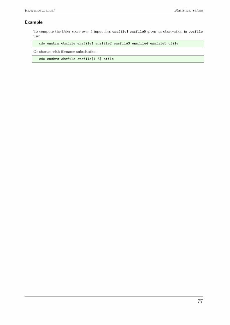
Reference manual Statistical values
Example
To compute the Brier score over 5 input files ensfile1-ensfile5 given an observation in obsfileuse:
cdo ensbrs obsfile ensfile1 ensfile2 ensfile3 ensfile4 ensfile5 ofile
Or shorter with filename substitution:
cdo ensbrs obsfile ensfile[1-5] ofile
77
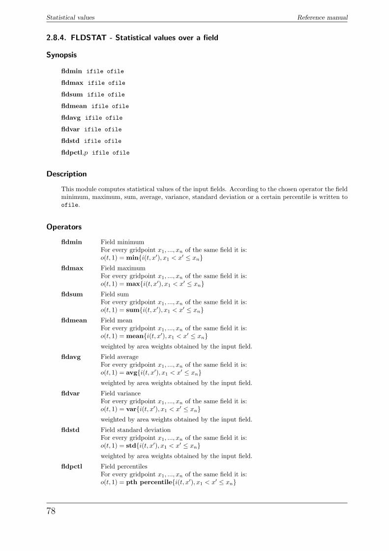
Statistical values Reference manual
2.8.4. FLDSTAT - Statistical values over a field
Synopsis
fldmin ifile ofile
fldmax ifile ofile
fldsum ifile ofile
fldmean ifile ofile
fldavg ifile ofile
fldvar ifile ofile
fldstd ifile ofile
fldpctl,p ifile ofile
Description
This module computes statistical values of the input fields. According to the chosen operator the fieldminimum, maximum, sum, average, variance, standard deviation or a certain percentile is written toofile.
Operators
fldmin Field minimumFor every gridpoint x1, ..., xn of the same field it is:o(t, 1) = min{i(t, x′), x1 < x′ ≤ xn}
fldmax Field maximumFor every gridpoint x1, ..., xn of the same field it is:o(t, 1) = max{i(t, x′), x1 < x′ ≤ xn}
fldsum Field sumFor every gridpoint x1, ..., xn of the same field it is:o(t, 1) = sum{i(t, x′), x1 < x′ ≤ xn}
fldmean Field meanFor every gridpoint x1, ..., xn of the same field it is:o(t, 1) = mean{i(t, x′), x1 < x′ ≤ xn}weighted by area weights obtained by the input field.
fldavg Field averageFor every gridpoint x1, ..., xn of the same field it is:o(t, 1) = avg{i(t, x′), x1 < x′ ≤ xn}weighted by area weights obtained by the input field.
fldvar Field varianceFor every gridpoint x1, ..., xn of the same field it is:o(t, 1) = var{i(t, x′), x1 < x′ ≤ xn}weighted by area weights obtained by the input field.
fldstd Field standard deviationFor every gridpoint x1, ..., xn of the same field it is:o(t, 1) = std{i(t, x′), x1 < x′ ≤ xn}weighted by area weights obtained by the input field.
fldpctl Field percentilesFor every gridpoint x1, ..., xn of the same field it is:o(t, 1) = pth percentile{i(t, x′), x1 < x′ ≤ xn}
78
Reference manual Statistical values
Parameter
p FLOAT Percentile number in 0, ..., 100
Example
To compute the field mean of all input fields use:
cdo fldmean ifile ofile
To compute the 90th percentile of all input fields use:
cdo fldpctl,90 ifile ofile
79
Statistical values Reference manual
2.8.5. ZONSTAT - Zonal statistical values
Synopsis
zonmin ifile ofile
zonmax ifile ofile
zonsum ifile ofile
zonmean ifile ofile
zonavg ifile ofile
zonvar ifile ofile
zonstd ifile ofile
zonpctl,p ifile ofile
Description
This module computes zonal statistical values of the input fields. According to the chosen operatorthe zonal minimum, maximum, sum, average, variance, standard deviation or a certain percentile iswritten to ofile. All input fields need to have the same regular lonlat grid.
Operators
zonmin Zonal minimumFor every latitude the minimum over all longitudes is computed.
zonmax Zonal maximumFor every latitude the maximum over all longitudes is computed.
zonsum Zonal sumFor every latitude the sum over all longitudes is computed.
zonmean Zonal meanFor every latitude the mean over all longitudes is computed.
zonavg Zonal averageFor every latitude the average over all longitudes is computed.
zonvar Zonal varianceFor every latitude the variance over all longitudes is computed.
zonstd Zonal standard deviationFor every latitude the standard deviation over all longitudes is computed.
zonpctl Zonal percentilesFor every latitude the pth percentile over all longitudes is computed.
Parameter
p FLOAT Percentile number in 0, ..., 100
80
Reference manual Statistical values
Example
To compute the zonal mean of all input fields use:
cdo zonmean ifile ofile
To compute the 50th meridional percentile (median) of all input fields use:
cdo zonpctl,50 ifile ofile
81
Statistical values Reference manual
2.8.6. MERSTAT - Meridional statistical values
Synopsis
mermin ifile ofile
mermax ifile ofile
mersum ifile ofile
mermean ifile ofile
meravg ifile ofile
mervar ifile ofile
merstd ifile ofile
merpctl,p ifile ofile
Description
This module computes meridional statistical values of the input fields. According to the chosenoperator the meridional minimum, maximum, sum, average, variance, standard deviation or a certainpercentile is written to ofile. All input fields need to have the same regular lon/lat grid.
Operators
mermin Meridional minimumFor every longitude the minimum over all latitudes is computed.
mermax Meridional maximumFor every longitude the maximum over all latitudes is computed.
mersum Meridional sumFor every longitude the sum over all latitudes is computed.
mermean Meridional meanFor every longitude the area weighted mean over all latitudes is computed.
meravg Meridional averageFor every longitude the area weighted average over all latitudes is computed.
mervar Meridional varianceFor every longitude the variance over all latitudes is computed.
merstd Meridional standard deviationFor every longitude the standard deviation over all latitudes is computed.
merpctl Meridional percentilesFor every longitude the pth percentile over all latitudes is computed.
Parameter
p FLOAT Percentile number in 0, ..., 100
82
Reference manual Statistical values
Example
To compute the meridional mean of all input fields use:
cdo mermean ifile ofile
To compute the 50th meridional percentile (median) of all input fields use:
cdo merpctl,50 ifile ofile
83
Statistical values Reference manual
2.8.7. GRIDBOXSTAT - Statistical values over grid boxes
Synopsis
<operator>,nx,,ny ifile ofile
Description
This module computes statistical values over surrounding grid boxes. According to the chosen operatorthe minimum, maximum, sum, average, variance, or standard deviation of the neighboring grid boxesis written to ofile. All gridbox operators only works on quadrilateral curvilinear grids.
Operators
gridboxmin Gridbox minimum
gridboxmax Gridbox maximum
gridboxsum Gridbox sum
gridboxmean Gridbox mean
gridboxavg Gridbox average
gridboxvar Gridbox variance
gridboxstd Gridbox standard deviation
Parameter
nx INTEGER Number of grid boxes in x direction
ny INTEGER Number of grid boxes in y direction
Example
To compute the mean over 10x10 grid boxes of the input field use:
cdo gridboxmean,10,10 ifile ofile
84
Reference manual Statistical values
2.8.8. VERTSTAT - Vertical statistical values
Synopsis
<operator> ifile ofile
Description
This module computes statistical values over all levels of the input variables. According to chosenoperator the vertical minimum, maximum, sum, average, variance or standard deviation is written toofile.
Operators
vertmin Vertical minimumFor every gridpoint the minimum over all levels is computed.
vertmax Vertical maximumFor every gridpoint the maximum over all levels is computed.
vertsum Vertical sumFor every gridpoint the sum over all levels is computed.
vertmean Vertical meanFor every gridpoint the mean over all levels is computed.
vertavg Vertical averageFor every gridpoint the average over all levels is computed.
vertvar Vertical varianceFor every gridpoint the variance over all levels is computed.
vertstd Vertical standard deviationFor every gridpoint the standard deviation over all levels is computed.
Example
To compute the vertical sum of all input variables use:
cdo vertsum ifile ofile
85
Statistical values Reference manual
2.8.9. TIMSELSTAT - Time range statistical values
Synopsis
<operator>,nsets[,noffset[,nskip]] ifile ofile
Description
This module computes statistical values for a selected number of time steps. According to the chosenoperator the minimum, maximum, sum, average, variance or standard deviation of the selected timesteps is written to ofile. The date information of a time step in ofile is the date of the lastcontributing time step in ifile.
Operators
timselmin Time range minimumFor every adjacent sequence t1, ..., tn of time steps of the same selected time rangeit is:o(t, x) = min{i(t′, x), t1 < t′ ≤ tn}
timselmax Time range maximumFor every adjacent sequence t1, ..., tn of time steps of the same selected time rangeit is:o(t, x) = max{i(t′, x), t1 < t′ ≤ tn}
timselsum Time range sumFor every adjacent sequence t1, ..., tn of time steps of the same selected time rangeit is:o(t, x) = sum{i(t′, x), t1 < t′ ≤ tn}
timselmean Time range meanFor every adjacent sequence t1, ..., tn of time steps of the same selected time rangeit is:o(t, x) = mean{i(t′, x), t1 < t′ ≤ tn}
timselavg Time range averageFor every adjacent sequence t1, ..., tn of time steps of the same selected time rangeit is:o(t, x) = avg{i(t′, x), t1 < t′ ≤ tn}
timselvar Time range varianceFor every adjacent sequence t1, ..., tn of time steps of the same selected time rangeit is:o(t, x) = var{i(t′, x), t1 < t′ ≤ tn}
timselstd Time range standard deviationFor every adjacent sequence t1, ..., tn of time steps of the same selected time rangeit is:o(t, x) = std{i(t′, x), t1 < t′ ≤ tn}
Parameter
nsets INTEGER Number of input time steps for each output time step
noffset INTEGER Number of input time steps skipped before the first time step range (optional)
nskip INTEGER Number of input time steps skipped between time step ranges (optional)
86
Reference manual Statistical values
Example
Assume an input dataset has monthly means over several years. To compute seasonal means frommonthly means the first two month have to be skipped:
cdo timselmean,3,2 ifile ofile
2.8.10. TIMSELPCTL - Time range percentile values
Synopsis
timselpctl,p,nsets[,noffset[,nskip]] ifile1 ifile2 ifile3 ofile
Description
This operator computes percentile values over a selected number of time steps in ifile1. The algo-rithm uses histograms with minimum and maximum bounds given in ifile2 and ifile3, respectively.The default number of histogram bins is 101. The default can be overridden by setting the environ-ment variable CDO PCTL NBINS to a different value. The files ifile2 and ifile3 should be the resultof corresponding timselmin and timselmax operations, respectively. The date information of a timestep in ofile is the date of the last contributing time step in ifile.For every adjacent sequence t1, ..., tn of time steps of the same selected time range it is:
o(t, x) = pth percentile{i(t′, x), t1 < t′ ≤ tn}
Parameter
p FLOAT Percentile number in 0, ..., 100
nsets INTEGER Number of input time steps for each output time step
noffset INTEGER Number of input time steps skipped before the first time step range (optional)
nskip INTEGER Number of input time steps skipped between time step ranges (optional)
Environment
CDO PCTL NBINS Sets the number of histogram bins. The default number is 101.
87
Statistical values Reference manual
2.8.11. RUNSTAT - Running statistical values
Synopsis
<operator>,nts ifile ofile
Description
This module computes running statistical values over a selected number of time steps. Dependingon the chosen operator the minimum, maximum, sum, average, variance or standard deviation of aselected number of consecutive time steps read from ifile is written to ofile. The date informationin ofile is the date of the middle contributing time step in ifile.
Operators
runmin Running minimumo(t + (nts− 1)/2, x) = min{i(t, x), i(t + 1, x), ..., i(t + nts− 1, x)}
runmax Running maximumo(t + (nts− 1)/2, x) = max{i(t, x), i(t + 1, x), ..., i(t + nts− 1, x)}
runsum Running sumo(t + (nts− 1)/2, x) = sum{i(t, x), i(t + 1, x), ..., i(t + nts− 1, x)}
runmean Running meano(t + (nts− 1)/2, x) = mean{i(t, x), i(t + 1, x), ..., i(t + nts− 1, x)}
runavg Running averageo(t + (nts− 1)/2, x) = avg{i(t, x), i(t + 1, x), ..., i(t + nts− 1, x)}
runvar Running varianceo(t + (nts− 1)/2, x) = std{i(t, x), i(t + 1, x), ..., i(t + nts− 1, x)}
runstd Running standard deviationo(t + (nts− 1)/2, x) = std{i(t, x), i(t + 1, x), ..., i(t + nts− 1, x)}
Parameter
nts INTEGER Number of time steps
Environment
RUNSTAT DATE Sets the date information in ofile to the ”first”, ”last” or ”middle” contributingtime step in ifile.
Example
To compute the running mean over 9 time steps use:
cdo runmean,9 ifile ofile
88
Reference manual Statistical values
2.8.12. RUNPCTL - Running percentile values
Synopsis
runpctl,p,nts ifile1 ofile
Description
This module computes running percentiles over a selected number of time steps in ifile1. The dateinformation in ofile is the date of the medium contributing time step in ifile1.
o(t + (nts− 1)/2, x) = pth percentile{i(t, x), i(t + 1, x), ..., i(t + nts− 1, x)}
Parameter
p FLOAT Percentile number in 0, ..., 100
nts INTEGER Number of time steps
Example
To compute the running 50th percentile (median) over 9 time steps use:
cdo runpctl,50,9 ifile -runmin,9 ifile -runmax,9 ifile ofile
89
Statistical values Reference manual
2.8.13. TIMSTAT - Statistical values over all time steps
Synopsis
<operator> ifile ofile
Description
This module computes statistical values over all time steps in ifile. Depending on the chosenoperator the minimum, maximum, sum, average, variance or standard deviation of all time steps readfrom ifile is written to ofile. The date information of a time step in ofile is the date of the lastcontributing time step in ifile.
Operators
timmin Time minimumo(1, x) = min{i(t′, x), t1 < t′ ≤ tn}
timmax Time maximumo(1, x) = max{i(t′, x), t1 < t′ ≤ tn}
timsum Time sumo(1, x) = sum{i(t′, x), t1 < t′ ≤ tn}
timmean Time meano(1, x) = mean{i(t′, x), t1 < t′ ≤ tn}
timavg Time averageo(1, x) = avg{i(t′, x), t1 < t′ ≤ tn}
timvar Time varianceo(1, x) = var{i(t′, x), t1 < t′ ≤ tn}
timstd Time standard deviationo(1, x) = std{i(t′, x), t1 < t′ ≤ tn}
Example
To compute the mean over all input time steps use:
cdo timmean ifile ofile
90
Reference manual Statistical values
2.8.14. TIMPCTL - Percentile values over all time steps
Synopsis
timpctl,p ifile1 ifile2 ifile3 ofile
Description
This operator computes percentiles over all time steps in ifile1. The algorithm uses histogramswith minimum and maximum bounds given in ifile2 and ifile3, respectively. The default num-ber of histogram bins is 101. The default can be overridden by setting the environment variableCDO PCTL NBINS to a different value. The files ifile2 and ifile3 should be the result of correspond-ing timmin and timmax operations, respectively. The date information of a time step in ofile is thedate of the last contributing time step in ifile1.
o(1, x) = pth percentile{i(t′, x), t1 < t′ ≤ tn}
Parameter
p FLOAT Percentile number in 0, ..., 100
Environment
CDO PCTL NBINS Sets the number of histogram bins. The default number is 101.
Example
To compute the 90th percentile over all input time steps use:
cdo timmin ifile minfilecdo timmax ifile maxfilecdo timpctl,90 ifile minfile maxfile ofile
Or shorter using operator piping:
cdo timpctl,90 ifile -timmin ifile -timmax ifile ofile
91
Statistical values Reference manual
2.8.15. HOURSTAT - Hourly statistical values
Synopsis
<operator> ifile ofile
Description
This module computes statistical values over time steps of the same hour. Depending on the chosenoperator the minimum, maximum, sum, average, variance or standard deviation of time steps of thesame hour is written to ofile. The date information of a time step in ofile is the date of the lastcontributing time step in ifile.
Operators
hourmin Hourly minimumFor every adjacent sequence t1, ..., tn of time steps of the same hour it is:o(t, x) = min{i(t′, x), t1 < t′ ≤ tn}
hourmax Hourly maximumFor every adjacent sequence t1, ..., tn of time steps of the same hour it is:o(t, x) = max{i(t′, x), t1 < t′ ≤ tn}
hoursum Hourly sumFor every adjacent sequence t1, ..., tn of time steps of the same hour it is:o(t, x) = sum{i(t′, x), t1 < t′ ≤ tn}
hourmean Hourly meanFor every adjacent sequence t1, ..., tn of time steps of the same hour it is:o(t, x) = mean{i(t′, x), t1 < t′ ≤ tn}
houravg Hourly averageFor every adjacent sequence t1, ..., tn of time steps of the same hour it is:o(t, x) = avg{i(t′, x), t1 < t′ ≤ tn}
hourvar Hourly varianceFor every adjacent sequence t1, ..., tn of time steps of the same hour it is:o(t, x) = var{i(t′, x), t1 < t′ ≤ tn}
hourstd Hourly standard deviationFor every adjacent sequence t1, ..., tn of time steps of the same hour it is:o(t, x) = std{i(t′, x), t1 < t′ ≤ tn}
Example
To compute the hourly mean of a time series use:
cdo hourmean ifile ofile
92
Reference manual Statistical values
2.8.16. HOURPCTL - Hourly percentile values
Synopsis
hourpctl,p ifile1 ifile2 ifile3 ofile
Description
This operator computes percentiles over all time steps of the same hour in ifile1. The algorithmuses histograms with minimum and maximum bounds given in ifile2 and ifile3, respectively. Thedefault number of histogram bins is 101. The default can be overridden by setting the environmentvariable CDO PCTL NBINS to a different value. The files ifile2 and ifile3 should be the result ofcorresponding hourmin and hourmax operations, respectively. The date information of a time step inofile is the date of the last contributing time step in ifile1.For every adjacent sequence t1, ..., tn of time steps of the same hour it is:
o(t, x) = pth percentile{i(t′, x), t1 < t′ ≤ tn}
Parameter
p FLOAT Percentile number in 0, ..., 100
Environment
CDO PCTL NBINS Sets the number of histogram bins. The default number is 101.
Example
To compute the hourly 90th percentile of a time series use:
cdo hourmin ifile minfilecdo hourmax ifile maxfilecdo hourpctl,90 ifile minfile maxfile ofile
Or shorter using operator piping:
cdo hourpctl,90 ifile -hourmin ifile -hourmax ifile ofile
93
Statistical values Reference manual
2.8.17. DAYSTAT - Daily statistical values
Synopsis
<operator> ifile ofile
Description
This module computes statistical values over time steps of the same day. Depending on the chosenoperator the minimum, maximum, sum, average, variance or standard deviation of time steps of thesame day is written to ofile. The date information of a time step in ofile is the date of the lastcontributing time step in ifile.
Operators
daymin Daily minimumFor every adjacent sequence t1, ..., tn of time steps of the same day it is:o(t, x) = min{i(t′, x), t1 < t′ ≤ tn}
daymax Daily maximumFor every adjacent sequence t1, ..., tn of time steps of the same day it is:o(t, x) = max{i(t′, x), t1 < t′ ≤ tn}
daysum Daily sumFor every adjacent sequence t1, ..., tn of time steps of the same day it is:o(t, x) = sum{i(t′, x), t1 < t′ ≤ tn}
daymean Daily meanFor every adjacent sequence t1, ..., tn of time steps of the same day it is:o(t, x) = mean{i(t′, x), t1 < t′ ≤ tn}
dayavg Daily averageFor every adjacent sequence t1, ..., tn of time steps of the same day it is:o(t, x) = avg{i(t′, x), t1 < t′ ≤ tn}
dayvar Daily varianceFor every adjacent sequence t1, ..., tn of time steps of the same day it is:o(t, x) = var{i(t′, x), t1 < t′ ≤ tn}
daystd Daily standard deviationFor every adjacent sequence t1, ..., tn of time steps of the same day it is:o(t, x) = std{i(t′, x), t1 < t′ ≤ tn}
Example
To compute the daily mean of a time series use:
cdo daymean ifile ofile
94
Reference manual Statistical values
2.8.18. DAYPCTL - Daily percentile values
Synopsis
daypctl,p ifile1 ifile2 ifile3 ofile
Description
This operator computes percentiles over all time steps of the same day in ifile1. The algorithmuses histograms with minimum and maximum bounds given in ifile2 and ifile3, respectively. Thedefault number of histogram bins is 101. The default can be overridden by defining the environmentvariable CDO PCTL NBINS. The files ifile2 and ifile3 should be the result of corresponding dayminand daymax operations, respectively. The date information of a time step in ofile is the date of thelast contributing time step in ifile1.For every adjacent sequence t1, ..., tn of time steps of the same day it is:
o(t, x) = pth percentile{i(t′, x), t1 < t′ ≤ tn}
Parameter
p FLOAT Percentile number in 0, ..., 100
Environment
CDO PCTL NBINS Sets the number of histogram bins. The default number is 101.
Example
To compute the daily 90th percentile of a time series use:
cdo daymin ifile minfilecdo daymax ifile maxfilecdo daypctl,90 ifile minfile maxfile ofile
Or shorter using operator piping:
cdo daypctl,90 ifile -daymin ifile -daymax ifile ofile
95
Statistical values Reference manual
2.8.19. MONSTAT - Monthly statistical values
Synopsis
<operator> ifile ofile
Description
This module computes statistical values over time steps of the same month. Depending on the chosenoperator the minimum, maximum, sum, average, variance or standard deviation of time steps of thesame month is written to ofile. The date information of a time step in ofile is the date of the lastcontributing time step in ifile.
Operators
monmin Monthly minimumFor every adjacent sequence t1, ..., tn of time steps of the same month it is:o(t, x) = min{i(t′, x), t1 < t′ ≤ tn}
monmax Monthly maximumFor every adjacent sequence t1, ..., tn of time steps of the same month it is:o(t, x) = max{i(t′, x), t1 < t′ ≤ tn}
monsum Monthly sumFor every adjacent sequence t1, ..., tn of time steps of the same month it is:o(t, x) = sum{i(t′, x), t1 < t′ ≤ tn}
monmean Monthly meanFor every adjacent sequence t1, ..., tn of time steps of the same month it is:o(t, x) = mean{i(t′, x), t1 < t′ ≤ tn}
monavg Monthly averageFor every adjacent sequence t1, ..., tn of time steps of the same month it is:o(t, x) = avg{i(t′, x), t1 < t′ ≤ tn}
monvar Monthly varianceFor every adjacent sequence t1, ..., tn of time steps of the same month it is:o(t, x) = var{i(t′, x), t1 < t′ ≤ tn}
monstd Monthly standard deviationFor every adjacent sequence t1, ..., tn of time steps of the same month it is:o(t, x) = std{i(t′, x), t1 < t′ ≤ tn}
Example
To compute the monthly mean of a time series use:
cdo monmean ifile ofile
96
Reference manual Statistical values
2.8.20. MONPCTL - Monthly percentile values
Synopsis
monpctl,p ifile1 ifile2 ifile3 ofile
Description
This operator computes percentiles over all time steps of the same month in ifile1. The algorithmuses histograms with minimum and maximum bounds given in ifile2 and ifile3, respectively. Thedefault number of histogram bins is 101. The default can be overridden by setting the environmentvariable CDO PCTL NBINS to a different value. The files ifile2 and ifile3 should be the result ofcorresponding monmin and monmax operations, respectively. The date information of a time step inofile is the date of the last contributing time step in ifile1.For every adjacent sequence t1, ..., tn of time steps of the same month it is:
o(t, x) = pth percentile{i(t′, x), t1 < t′ ≤ tn}
Parameter
p FLOAT Percentile number in 0, ..., 100
Environment
CDO PCTL NBINS Sets the number of histogram bins. The default number is 101.
Example
To compute the monthly 90th percentile of a time series use:
cdo monmin ifile minfilecdo monmax ifile maxfilecdo monpctl,90 ifile minfile maxfile ofile
Or shorter using operator piping:
cdo monpctl,90 ifile -monmin ifile -monmax ifile ofile
97
Statistical values Reference manual
2.8.21. YEARSTAT - Yearly statistical values
Synopsis
<operator> ifile ofile
Description
This module computes statistical values over time steps of the same year. Depending on the chosenoperator the minimum, maximum, sum, average, variance or standard deviation of time steps of thesame year is written to ofile. The date information of a time step in ofile is the date of the lastcontributing time step in ifile.
Operators
yearmin Yearly minimumFor every adjacent sequence t1, ..., tn of time steps of the same year it is:o(t, x) = min{i(t′, x), t1 < t′ ≤ tn}
yearmax Yearly maximumFor every adjacent sequence t1, ..., tn of time steps of the same year it is:o(t, x) = max{i(t′, x), t1 < t′ ≤ tn}
yearsum Yearly sumFor every adjacent sequence t1, ..., tn of time steps of the same year it is:o(t, x) = sum{i(t′, x), t1 < t′ ≤ tn}
yearmean Yearly meanFor every adjacent sequence t1, ..., tn of time steps of the same year it is:o(t, x) = mean{i(t′, x), t1 < t′ ≤ tn}
yearavg Yearly averageFor every adjacent sequence t1, ..., tn of time steps of the same year it is:o(t, x) = avg{i(t′, x), t1 < t′ ≤ tn}
yearvar Yearly varianceFor every adjacent sequence t1, ..., tn of time steps of the same year it is:o(t, x) = var{i(t′, x), t1 < t′ ≤ tn}
yearstd Yearly standard deviationFor every adjacent sequence t1, ..., tn of time steps of the same year it is:o(t, x) = std{i(t′, x), t1 < t′ ≤ tn}
Note
The operators yearmean and yearavg compute only arithmetical means!
Example
To compute the yearly mean of a time series use:
cdo yearmean ifile ofile
To compute the yearly mean from the correct weighted monthly mean use:
cdo divdpy -yearsum -muldpm ifile ofile
98

Reference manual Statistical values
2.8.22. YEARPCTL - Yearly percentile values
Synopsis
yearpctl,p ifile1 ifile2 ifile3 ofile
Description
This operator computes percentiles over all time steps of the same year in ifile1. The algorithmuses histograms with minimum and maximum bounds given in ifile2 and ifile3, respectively. Thedefault number of histogram bins is 101. The default can be overridden by setting the environmentvariable CDO PCTL NBINS to a different value. The files ifile2 and ifile3 should be the result ofcorresponding yearmin and yearmax operations, respectively. The date information of a time step inofile is the date of the last contributing time step in ifile1.For every adjacent sequence t1, ..., tn of time steps of the same year it is:
o(t, x) = pth percentile{i(t′, x), t1 < t′ ≤ tn}
Parameter
p FLOAT Percentile number in 0, ..., 100
Environment
CDO PCTL NBINS Sets the number of histogram bins. The default number is 101.
Example
To compute the yearly 90th percentile of a time series use:
cdo yearmin ifile minfilecdo yearmax ifile maxfilecdo yearpctl,90 ifile minfile maxfile ofile
Or shorter using operator piping:
cdo yearpctl,90 ifile -yearmin ifile -yearmax ifile ofile
99
Statistical values Reference manual
2.8.23. SEASSTAT - Seasonal statistical values
Synopsis
<operator> ifile ofile
Description
This module computes statistical values over time steps of the same season. Depending on the chosenoperator the minimum, maximum, sum, average, variance or standard deviation of time steps of thesame season is written to ofile. The date information of a time step in ofile is the date of the lastcontributing time step in ifile. Be careful about the first and the last output time step, they maybe incorrect values if the seasons have incomplete time steps.
Operators
seasmin Seasonal minimumFor every adjacent sequence t1, ..., tn of time steps of the same season it is:o(t, x) = min{i(t′, x), t1 < t′ ≤ tn}
seasmax Seasonal maximumFor every adjacent sequence t1, ..., tn of time steps of the same season it is:o(t, x) = max{i(t′, x), t1 < t′ ≤ tn}
seassum Seasonal sumFor every adjacent sequence t1, ..., tn of time steps of the same season it is:o(t, x) = sum{i(t′, x), t1 < t′ ≤ tn}
seasmean Seasonal meanFor every adjacent sequence t1, ..., tn of time steps of the same season it is:o(t, x) = mean{i(t′, x), t1 < t′ ≤ tn}
seasavg Seasonal averageFor every adjacent sequence t1, ..., tn of time steps of the same season it is:o(t, x) = avg{i(t′, x), t1 < t′ ≤ tn}
seasvar Seasonal varianceFor every adjacent sequence t1, ..., tn of time steps of the same season it is:o(t, x) = var{i(t′, x), t1 < t′ ≤ tn}
seasstd Seasonal standard deviationFor every adjacent sequence t1, ..., tn of time steps of the same season it is:o(t, x) = std{i(t′, x), t1 < t′ ≤ tn}
Example
To compute the seasonal mean of a time series use:
cdo seasmean ifile ofile
100
Reference manual Statistical values
2.8.24. SEASPCTL - Seasonal percentile values
Synopsis
seaspctl,p ifile1 ifile2 ifile3 ofile
Description
This operator computes percentiles over all time steps in ifile1 of the same season. The algorithmuses histograms with minimum and maximum bounds given in ifile2 and ifile3, respectively. Thedefault number of histogram bins is 101. The default can be overridden by setting the environmentvariable CDO PCTL NBINS to a different value. The files ifile2 and ifile3 should be the result ofcorresponding seasmin and seasmax operations, respectively. The date information of a time step inofile is the date of the last contributing time step in ifile1. Be careful about the first and the lastoutput time step, they may be incorrect values if the seasons have incomplete time steps.For every adjacent sequence t1, ..., tn of time steps of the same season it is:
o(t, x) = pth percentile{i(t′, x), t1 < t′ ≤ tn}
Parameter
p FLOAT Percentile number in 0, ..., 100
Environment
CDO PCTL NBINS Sets the number of histogram bins. The default number is 101.
Example
To compute the seasonal 90th percentile of a time series use:
cdo seasmin ifile minfilecdo seasmax ifile maxfilecdo seaspctl,90 ifile minfile maxfile ofile
Or shorter using operator piping:
cdo seaspctl,90 ifile -seasmin ifile -seasmax ifile ofile
101
Statistical values Reference manual
2.8.25. YHOURSTAT - Multi-year hourly statistical values
Synopsis
<operator> ifile ofile
Description
This module computes statistical values of each hour and day of year. Depending on the chosenoperator the minimum, maximum, sum, average, variance or standard deviation of each hour and dayof year in ifile is written to ofile. The date information in an output field is the date of the lastcontributing input field.
Operators
yhourmin Multi-year hourly minimumo(0001, x) = min{i(t, x),day(i(t)) = 0001}
...o(8784, x) = min{i(t, x),day(i(t)) = 8784}
yhourmax Multi-year hourly maximumo(0001, x) = max{i(t, x),day(i(t)) = 0001}
...o(8784, x) = max{i(t, x),day(i(t)) = 8784}
yhoursum Multi-year hourly sumo(0001, x) = sum{i(t, x),day(i(t)) = 0001}
...o(8784, x) = sum{i(t, x),day(i(t)) = 8784}
yhourmean Multi-year hourly meano(0001, x) = mean{i(t, x),day(i(t)) = 0001}
...o(8784, x) = mean{i(t, x),day(i(t)) = 8784}
yhouravg Multi-year hourly averageo(0001, x) = avg{i(t, x),day(i(t)) = 0001}
...o(8784, x) = avg{i(t, x),day(i(t)) = 8784}
yhourvar Multi-year hourly varianceo(0001, x) = var{i(t, x),day(i(t)) = 0001}
...o(8784, x) = var{i(t, x),day(i(t)) = 8784}
yhourstd Multi-year hourly standard deviationo(0001, x) = std{i(t, x),day(i(t)) = 0001}
...o(8784, x) = std{i(t, x),day(i(t)) = 8784}
Example
To compute the hourly mean for all days over all input years use:
cdo yhourmean ifile ofile
102
Reference manual Statistical values
2.8.26. YDAYSTAT - Multi-year daily statistical values
Synopsis
<operator> ifile ofile
Description
This module computes statistical values of each day of year. Depending on the chosen operator theminimum, maximum, sum, average, variance or standard deviation of each day of year in ifile iswritten to ofile. The date information in an output field is the date of the last contributing inputfield.
Operators
ydaymin Multi-year daily minimumo(001, x) = min{i(t, x),day(i(t)) = 001}
...o(366, x) = min{i(t, x),day(i(t)) = 366}
ydaymax Multi-year daily maximumo(001, x) = max{i(t, x),day(i(t)) = 001}
...o(366, x) = max{i(t, x),day(i(t)) = 366}
ydaysum Multi-year daily sumo(001, x) = sum{i(t, x),day(i(t)) = 001}
...o(366, x) = sum{i(t, x),day(i(t)) = 366}
ydaymean Multi-year daily meano(001, x) = mean{i(t, x),day(i(t)) = 001}
...o(366, x) = mean{i(t, x),day(i(t)) = 366}
ydayavg Multi-year daily averageo(001, x) = avg{i(t, x),day(i(t)) = 001}
...o(366, x) = avg{i(t, x),day(i(t)) = 366}
ydayvar Multi-year daily varianceo(001, x) = var{i(t, x),day(i(t)) = 001}
...o(366, x) = var{i(t, x),day(i(t)) = 366}
ydaystd Multi-year daily standard deviationo(001, x) = std{i(t, x),day(i(t)) = 001}
...o(366, x) = std{i(t, x),day(i(t)) = 366}
Example
To compute the daily mean over all input years use:
cdo ydaymean ifile ofile
103
Statistical values Reference manual
2.8.27. YDAYPCTL - Multi-year daily percentile values
Synopsis
ydaypctl,p ifile1 ifile2 ifile3 ofile
Description
This operator writes a certain percentile of each day of year in ifile1 to ofile. The algorithmuses histograms with minimum and maximum bounds given in ifile2 and ifile3, respectively. Thedefault number of histogram bins is 101. The default can be overridden by setting the environmentvariable CDO PCTL NBINS to a different value. The files ifile2 and ifile3 should be the result ofcorresponding ydaymin and ydaymax operations, respectively. The date information in an outputfield is the date of the last contributing input field.
o(001, x) = pth percentile{i(t, x),day(i(t)) = 001}...
o(366, x) = pth percentile{i(t, x),day(i(t)) = 366}
Parameter
p FLOAT Percentile number in 0, ..., 100
Environment
CDO PCTL NBINS Sets the number of histogram bins. The default number is 101.
Example
To compute the daily 90th percentile over all input years use:
cdo ydaymin ifile minfilecdo ydaymax ifile maxfilecdo ydaypctl,90 ifile minfile maxfile ofile
Or shorter using operator piping:
cdo ydaypctl,90 ifile -ydaymin ifile -ydaymax ifile ofile
104
Reference manual Statistical values
2.8.28. YMONSTAT - Multi-year monthly statistical values
Synopsis
<operator> ifile ofile
Description
This module computes statistical values of each month of year. Depending on the chosen operator theminimum, maximum, sum, average, variance or standard deviation of each month of year in ifile iswritten to ofile. The date information in an output field is the date of the last contributing inputfield.
Operators
ymonmin Multi-year monthly minimumo(01, x) = min{i(t, x),month(i(t)) = 01}
...o(12, x) = min{i(t, x),month(i(t)) = 12}
ymonmax Multi-year monthly maximumo(01, x) = max{i(t, x),month(i(t)) = 01}
...o(12, x) = max{i(t, x),month(i(t)) = 12}
ymonsum Multi-year monthly sumo(01, x) = sum{i(t, x),month(i(t)) = 01}
...o(12, x) = sum{i(t, x),month(i(t)) = 12}
ymonmean Multi-year monthly meano(01, x) = mean{i(t, x),month(i(t)) = 01}
...o(12, x) = mean{i(t, x),month(i(t)) = 12}
ymonavg Multi-year monthly averageo(01, x) = avg{i(t, x),month(i(t)) = 01}
...o(12, x) = avg{i(t, x),month(i(t)) = 12}
ymonvar Multi-year monthly varianceo(01, x) = var{i(t, x),month(i(t)) = 01}
...o(12, x) = var{i(t, x),month(i(t)) = 12}
ymonstd Multi-year monthly standard deviationo(01, x) = std{i(t, x),month(i(t)) = 01}
...o(12, x) = std{i(t, x),month(i(t)) = 12}
Example
To compute the monthly mean over all input years use:
cdo ymonmean ifile ofile
105
Statistical values Reference manual
2.8.29. YMONPCTL - Multi-year monthly percentile values
Synopsis
ymonpctl,p ifile1 ifile2 ifile3 ofile
Description
This operator writes a certain percentile of each month of year in ifile1 to ofile. The algorithmuses histograms with minimum and maximum bounds given in ifile2 and ifile3, respectively. Thedefault number of histogram bins is 101. The default can be overridden by setting the environmentvariable CDO PCTL NBINS to a different value. The files ifile2 and ifile3 should be the result ofcorresponding ymonmin and ymonmax operations, respectively. The date information in an outputfield is the date of the last contributing input field.
o(01, x) = pth percentile{i(t, x),month(i(t)) = 01}...
o(12, x) = pth percentile{i(t, x),month(i(t)) = 12}
Parameter
p FLOAT Percentile number in 0, ..., 100
Environment
CDO PCTL NBINS Sets the number of histogram bins. The default number is 101.
Example
To compute the monthly 90th percentile over all input years use:
cdo ymonmin ifile minfilecdo ymonmax ifile maxfilecdo ymonpctl,90 ifile minfile maxfile ofile
Or shorter using operator piping:
cdo ymonpctl,90 ifile -ymonmin ifile -ymonmax ifile ofile
106
Reference manual Statistical values
2.8.30. YSEASSTAT - Multi-year seasonal statistical values
Synopsis
<operator> ifile ofile
Description
This module computes statistical values of each season. Depending on the chosen operator theminimum, maximum, sum, average, variance or standard deviation of each season in ifile is writtento ofile. The date information in an output field is the date of the last contributing input field.
Operators
yseasmin Multi-year seasonal minimumo(1, x) = min{i(t, x),month(i(t)) = 12, 01, 02}o(2, x) = min{i(t, x),month(i(t)) = 03, 04, 05}o(3, x) = min{i(t, x),month(i(t)) = 06, 07, 08}o(4, x) = min{i(t, x),month(i(t)) = 09, 10, 11}
yseasmax Multi-year seasonal maximumo(1, x) = max{i(t, x),month(i(t)) = 12, 01, 02}o(2, x) = max{i(t, x),month(i(t)) = 03, 04, 05}o(3, x) = max{i(t, x),month(i(t)) = 06, 07, 08}o(4, x) = max{i(t, x),month(i(t)) = 09, 10, 11}
yseassum Multi-year seasonal sumo(1, x) = sum{i(t, x),month(i(t)) = 12, 01, 02}o(2, x) = sum{i(t, x),month(i(t)) = 03, 04, 05}o(3, x) = sum{i(t, x),month(i(t)) = 06, 07, 08}o(4, x) = sum{i(t, x),month(i(t)) = 09, 10, 11}
yseasmean Multi-year seasonal meano(1, x) = mean{i(t, x),month(i(t)) = 12, 01, 02}o(2, x) = mean{i(t, x),month(i(t)) = 03, 04, 05}o(3, x) = mean{i(t, x),month(i(t)) = 06, 07, 08}o(4, x) = mean{i(t, x),month(i(t)) = 09, 10, 11}
yseasavg Multi-year seasonal averageo(1, x) = avg{i(t, x),month(i(t)) = 12, 01, 02}o(2, x) = avg{i(t, x),month(i(t)) = 03, 04, 05}o(3, x) = avg{i(t, x),month(i(t)) = 06, 07, 08}o(4, x) = avg{i(t, x),month(i(t)) = 09, 10, 11}
yseasvar Multi-year seasonal varianceo(1, x) = var{i(t, x),month(i(t)) = 12, 01, 02}o(2, x) = var{i(t, x),month(i(t)) = 03, 04, 05}o(3, x) = var{i(t, x),month(i(t)) = 06, 07, 08}o(4, x) = var{i(t, x),month(i(t)) = 09, 10, 11}
yseasstd Multi-year seasonal standard deviationo(1, x) = std{i(t, x),month(i(t)) = 12, 01, 02}o(2, x) = std{i(t, x),month(i(t)) = 03, 04, 05}o(3, x) = std{i(t, x),month(i(t)) = 06, 07, 08}o(4, x) = std{i(t, x),month(i(t)) = 09, 10, 11}
107
Statistical values Reference manual
Example
To compute the seasonal mean over all input years use:
cdo yseasmean ifile ofile
2.8.31. YSEASPCTL - Multi-year seasonal percentile values
Synopsis
yseaspctl,p ifile1 ifile2 ifile3 ofile
Description
This operator writes a certain percentile of each season in ifile1 to ofile. The algorithm useshistograms with minimum and maximum bounds given in ifile2 and ifile3, respectively. Thedefault number of histogram bins is 101. The default can be overridden by setting the environmentvariable CDO PCTL NBINS to a different value. The files ifile2 and ifile3 should be the result ofcorresponding yseasmin and yseasmax operations, respectively. The date information in an outputfield is the date of the last contributing input field.
o(1, x) = pth percentile{i(t, x),month(i(t)) = 12, 01, 02}o(2, x) = pth percentile{i(t, x),month(i(t)) = 03, 04, 05}o(3, x) = pth percentile{i(t, x),month(i(t)) = 06, 07, 08}o(4, x) = pth percentile{i(t, x),month(i(t)) = 09, 10, 11}
Parameter
p FLOAT Percentile number in 0, ..., 100
Environment
CDO PCTL NBINS Sets the number of histogram bins. The default number is 101.
Example
To compute the seasonal 90th percentile over all input years use:
cdo yseasmin ifile minfilecdo yseasmax ifile maxfilecdo yseaspctl,90 ifile minfile maxfile ofile
Or shorter using operator piping:
cdo yseaspctl,90 ifile -yseasmin ifile -yseasmax ifile ofile
108
Reference manual Statistical values
2.8.32. YDRUNSTAT - Multi-year daily running statistical values
Synopsis
<operator>,nts ifile ofile
Description
This module writes running statistical values for each day of year in ifile to ofile. Depending onthe chosen operator, the minimum, maximum, sum, average, variance or standard deviation of alltime steps in running windows of wich the medium time step corresponds to a certain day of year iscomputed. The date information in an output field is the date of the medium time step in the lastcontributing running window. Note that the operator have to be applied to a continuous time seriesof daily measurements in order to yield physically meaningful results. Also note that the output timeseries begins (nts-1)/2 time steps after the first time step of the input time series and ends (nts-1)/2time steps before the last one. For input data which are complete but not continuous, such as timeseries of daily measurements for the same month or season within different years, the operator yieldsphysically meaningful results only if the input time series does include the (nts-1)/2 days before andafter each period of interest.
Operators
ydrunmin Multi-year daily running minimumo(001, x) = min{i(t, x), i(t + 1, x), ..., i(t + nts− 1, x); day[(i(t + (nts− 1)/2)] = 001}
...o(366, x) = min{i(t, x), i(t + 1, x), ..., i(t + nts− 1, x); day[(i(t + (nts− 1)/2)] = 366}
ydrunmax Multi-year daily running maximumo(001, x) = max{i(t, x), i(t + 1, x), ..., i(t + nts− 1, x); day[(i(t + (nts− 1)/2)] = 001}
...o(366, x) = max{i(t, x), i(t + 1, x), ..., i(t + nts− 1, x); day[(i(t + (nts− 1)/2)] = 366}
ydrunsum Multi-year daily running sumo(001, x) = sum{i(t, x), i(t + 1, x), ..., i(t + nts− 1, x); day[(i(t + (nts− 1)/2)] = 001}
...o(366, x) = sum{i(t, x), i(t + 1, x), ..., i(t + nts− 1, x); day[(i(t + (nts− 1)/2)] = 366}
ydrunmean Multi-year daily running meano(001, x) = mean{i(t, x), i(t + 1, x), ..., i(t + nts− 1, x); day[(i(t + (nts− 1)/2)] = 001}
...o(366, x) = mean{i(t, x), i(t + 1, x), ..., i(t + nts− 1, x); day[(i(t + (nts− 1)/2)] = 366}
ydrunavg Multi-year daily running averageo(001, x) = avg{i(t, x), i(t + 1, x), ..., i(t + nts− 1, x); day[(i(t + (nts− 1)/2)] = 001}
...o(366, x) = avg{i(t, x), i(t + 1, x), ..., i(t + nts− 1, x); day[(i(t + (nts− 1)/2)] = 366}
ydrunvar Multi-year daily running varianceo(001, x) = var{i(t, x), i(t + 1, x), ..., i(t + nts− 1, x); day[(i(t + (nts− 1)/2)] = 001}
...o(366, x) = var{i(t, x), i(t + 1, x), ..., i(t + nts− 1, x); day[(i(t + (nts− 1)/2)] = 366}
ydrunstd Multi-year daily running standard deviationo(001, x) = std{i(t, x), i(t + 1, x), ..., i(t + nts− 1, x); day[(i(t + (nts− 1)/2)] = 001}
...o(366, x) = std{i(t, x), i(t + 1, x), ..., i(t + nts− 1, x); day[(i(t + (nts− 1)/2)] = 366}
109
Statistical values Reference manual
Parameter
nts INTEGER Number of time steps
Example
Assume the input data provide a continuous time series of daily measurements. To compute therunning multi-year daily mean over all input time steps for a running window of five days use:
cdo ydrunmean,5 ifile ofile
Note that except for the standard deviation the results of the operators in this module are equivalentto a composition of corresponding operators from the YDAYSTAT and RUNSTAT modules. Forinstance, the above command yields the same result as:
cdo ydaymean -runmean,5 ifile ofile
110
Reference manual Statistical values
2.8.33. YDRUNPCTL - Multi-year daily running percentile values
Synopsis
ydrunpctl,p,nts ifile1 ifile2 ifile3 ofile
Description
This operator writes running percentile values for each day of year in ifile1 to ofile. A certainpercentile is computed for all time steps in running windows of which the medium time step corre-sponds to a certain day of year. The algorithm uses histograms with minimum and maximum boundsgiven in ifile2 and ifile3, respectively. The default number of histogram bins is 101. The defaultcan be overridden by setting the environment variable CDO PCTL NBINS to a different value. Thefiles ifile2 and ifile3 should be the result of corresponding ydrunmin and ydrunmax operations,respectively. The date information in an output field is the date of the medium time step in the lastcontributing running window. Note that the operator have to be applied to a continuous time seriesof daily measurements in order to yield physically meaningful results. Also note that the output timeseries begins (nts-1)/2 time steps after the first time step of the input time series and ends (nts-1)/2time steps before the last. For input data which are complete but not continuous, such as time seriesof daily measurements for the same month or season within different years, the operator only yieldsphysically meaningful results if the input time series does include the (nts-1)/2 days before and aftereach period of interest.
o(001, x) = pth percentile{i(t, x), i(t + 1, x), ..., i(t + nts− 1, x); day[(i(t + (nts− 1)/2)] = 001}...
o(366, x) = pth percentile{i(t, x), i(t + 1, x), ..., i(t + nts− 1, x); day[(i(t + (nts− 1)/2)] = 366}
Parameter
p FLOAT Percentile number in 0, ..., 100
nts INTEGER Number of time steps
Environment
CDO PCTL NBINS Sets the number of histogram bins. The default number is 101.
Example
Assume the input data provide a continuous time series of daily measurements. To compute therunning multi-year daily 90th percentile over all input time steps for a running window of five daysuse:
cdo ydrunmin,5 ifile minfilecdo ydrunmax,5 ifile maxfilecdo ydrunpctl,90,5 ifile minfile maxfile ofile
Or shorter using operator piping:
cdo ydrunpctl,90,5 ifile -ydrunmin ifile -ydrunmax ifile ofile
111
Correlation Reference manual
2.9. Correlation
This sections contains modules for correlation in space and time.
Here is a short overview of all operators in this section:
fldcor Correlation in grid space
timcor Correlation over time
112
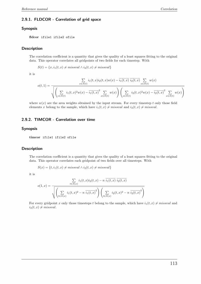
Reference manual Correlation
2.9.1. FLDCOR - Correlation of grid space
Synopsis
fldcor ifile1 ifile2 ofile
Description
The correlation coefficient is a quantity that gives the quality of a least squares fitting to the originaldata. This operator correlates all gridpoints of two fields for each timestep. With
S(t) = {x, i1(t, x) 6= missval ∧ i2(t, x) 6= missval}
it is
o(t, 1) =
∑x∈S(t)
i1(t, x)i2(t, x)w(x)− i1(t, x) i2(t, x)∑
x∈S(t)
w(x)√√√√( ∑x∈S(t)
i1(t, x)2w(x)− i1(t, x)2 ∑
x∈S(t)
w(x)
)( ∑x∈S(t)
i2(t, x)2w(x)− i2(t, x)2 ∑
x∈S(t)
w(x)
)
where w(x) are the area weights obtained by the input stream. For every timestep t only those fieldelements x belong to the sample, which have i1(t, x) 6= missval and i2(t, x) 6= missval.
2.9.2. TIMCOR - Correlation over time
Synopsis
timcor ifile1 ifile2 ofile
Description
The correlation coefficient is a quantity that gives the quality of a least squares fitting to the originaldata. This operator correlates each gridpoint of two fields over all timesteps. With
S(x) = {t, i1(t, x) 6= missval ∧ i2(t, x) 6= missval}
it is
o(1, x) =
∑t∈S(x)
i1(t, x)i2(t, x)− n i1(t, x) i2(t, x)√√√√( ∑t∈S(x)
i1(t, x)2 − n i1(t, x)2
)( ∑t∈S(x)
i2(t, x)2 − n i2(t, x)2
)
For every gridpoint x only those timesteps t belong to the sample, which have i1(t, x) 6= missval andi2(t, x) 6= missval.
113
Regression Reference manual
2.10. Regression
This sections contains modules for linear regression of time series.
Here is a short overview of all operators in this section:
regres Regression
detrend Detrend
trend Trend
subtrend Subtract trend
114
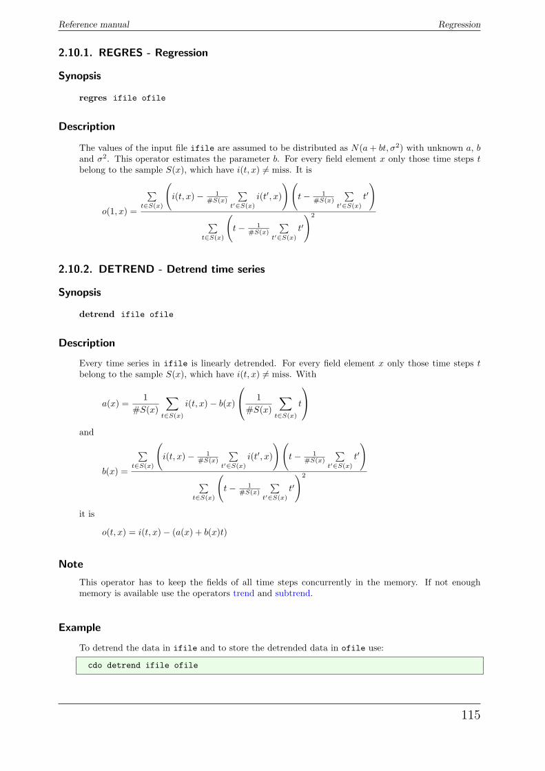
Reference manual Regression
2.10.1. REGRES - Regression
Synopsis
regres ifile ofile
Description
The values of the input file ifile are assumed to be distributed as N(a + bt, σ2) with unknown a, band σ2. This operator estimates the parameter b. For every field element x only those time steps tbelong to the sample S(x), which have i(t, x) 6= miss. It is
o(1, x) =
∑t∈S(x)
(i(t, x)− 1
#S(x)
∑t′∈S(x)
i(t′, x)
)(t− 1
#S(x)
∑t′∈S(x)
t′
)∑
t∈S(x)
(t− 1
#S(x)
∑t′∈S(x)
t′
)2
2.10.2. DETREND - Detrend time series
Synopsis
detrend ifile ofile
Description
Every time series in ifile is linearly detrended. For every field element x only those time steps tbelong to the sample S(x), which have i(t, x) 6= miss. With
a(x) =1
#S(x)
∑t∈S(x)
i(t, x)− b(x)
1#S(x)
∑t∈S(x)
t
and
b(x) =
∑t∈S(x)
(i(t, x)− 1
#S(x)
∑t′∈S(x)
i(t′, x)
)(t− 1
#S(x)
∑t′∈S(x)
t′
)∑
t∈S(x)
(t− 1
#S(x)
∑t′∈S(x)
t′
)2
it is
o(t, x) = i(t, x)− (a(x) + b(x)t)
Note
This operator has to keep the fields of all time steps concurrently in the memory. If not enoughmemory is available use the operators trend and subtrend.
Example
To detrend the data in ifile and to store the detrended data in ofile use:
cdo detrend ifile ofile
115
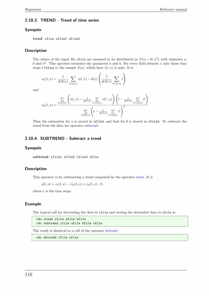
Regression Reference manual
2.10.3. TREND - Trend of time series
Synopsis
trend ifile ofile1 ofile2
Description
The values of the input file ifile are assumed to be distributed as N(a + bt, σ2) with unknown a,b and σ2. This operator estimates the parameter a and b. For every field element x only those timesteps t belong to the sample S(x), which have i(t, x) 6= miss. It is
o1(1, x) =1
#S(x)
∑t∈S(x)
i(t, x)− b(x)
1#S(x)
∑t∈S(x)
t
and
o2(1, x) =
∑t∈S(x)
(i(t, x)− 1
#S(x)
∑t′∈S(x)
i(t′, x)
)(t− 1
#S(x)
∑t′∈S(x)
t′
)∑
t∈S(x)
(t− 1
#S(x)
∑t′∈S(x)
t′
)2
Thus the estimation for a is stored in ofile1 and that for b is stored in ofile2. To subtract thetrend from the data see operator subtrend.
2.10.4. SUBTREND - Subtract a trend
Synopsis
subtrend ifile1 ifile2 ifile3 ofile
Description
This operator is for subtracting a trend computed by the operator trend. It is
o(t, x) = i1(t, x)− (i2(1, x) + i3(1, x) · t)
where t is the time steps.
Example
The typical call for detrending the data in ifile and storing the detrended data in ofile is:
cdo trend ifile afile bfilecdo subtrend ifile afile bfile ofile
The result is identical to a call of the operator detrend:
cdo detrend ifile ofile
116
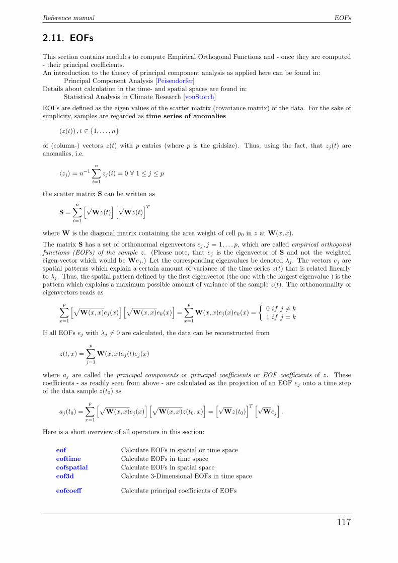
Reference manual EOFs
2.11. EOFs
This section contains modules to compute Empirical Orthogonal Functions and - once they are computed- their principal coefficients.An introduction to the theory of principal component analysis as applied here can be found in:
Principal Component Analysis [Peisendorfer]Details about calculation in the time- and spatial spaces are found in:
Statistical Analysis in Climate Research [vonStorch]
EOFs are defined as the eigen values of the scatter matrix (covariance matrix) of the data. For the sake ofsimplicity, samples are regarded as time series of anomalies
(z(t)) , t ∈ {1, . . . , n}
of (column-) vectors z(t) with p entries (where p is the gridsize). Thus, using the fact, that zj(t) areanomalies, i.e.
〈zj〉 = n−1n∑
i=1
zj(i) = 0 ∀ 1 ≤ j ≤ p
the scatter matrix S can be written as
S =n∑
t=1
[√Wz(t)
] [√Wz(t)
]Twhere W is the diagonal matrix containing the area weight of cell p0 in z at W(x, x).
The matrix S has a set of orthonormal eigenvectors ej , j = 1, . . . p, which are called empirical orthogonalfunctions (EOFs) of the sample z. (Please note, that ej is the eigenvector of S and not the weightedeigen-vector which would be Wej .) Let the corresponding eigenvalues be denoted λj . The vectors ej arespatial patterns which explain a certain amount of variance of the time series z(t) that is related linearlyto λj . Thus, the spatial pattern defined by the first eigenvector (the one with the largest eigenvalue ) is thepattern which explains a maximum possible amount of variance of the sample z(t). The orthonormality ofeigenvectors reads as
p∑x=1
[√W(x, x)ej(x)
] [√W(x, x)ek(x)
]=
p∑x=1
W(x, x)ej(x)ek(x) ={
0 if j 6= k
1 if j = k
If all EOFs ej with λj 6= 0 are calculated, the data can be reconstructed from
z(t, x) =p∑
j=1
W(x, x)aj(t)ej(x)
where aj are called the principal components or principal coefficients or EOF coefficients of z. Thesecoefficients - as readily seen from above - are calculated as the projection of an EOF ej onto a time stepof the data sample z(t0) as
aj(t0) =p∑
x=1
[√W(x, x)ej(x)
] [√W(x, x)z(t0, x)
]=[√
Wz(t0)]T [√
Wej
].
Here is a short overview of all operators in this section:
eof Calculate EOFs in spatial or time spaceeoftime Calculate EOFs in time spaceeofspatial Calculate EOFs in spatial spaceeof3d Calculate 3-Dimensional EOFs in time space
eofcoeff Calculate principal coefficients of EOFs
117
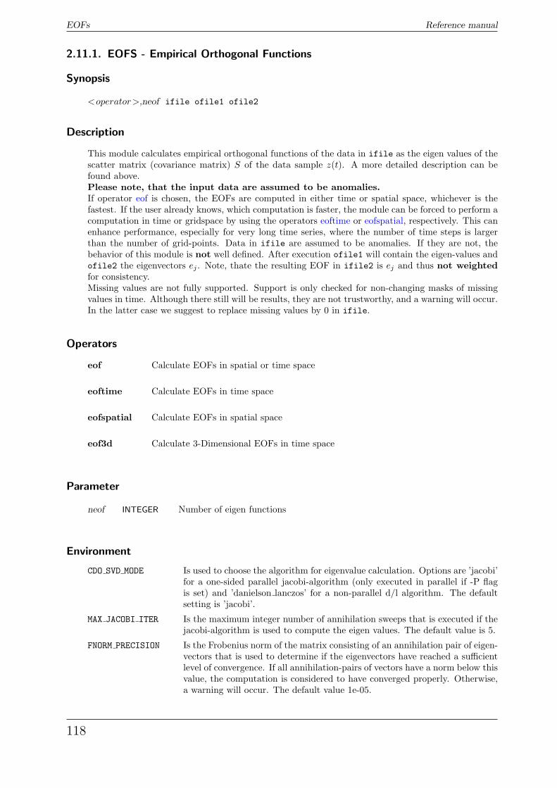
EOFs Reference manual
2.11.1. EOFS - Empirical Orthogonal Functions
Synopsis
<operator>,neof ifile ofile1 ofile2
Description
This module calculates empirical orthogonal functions of the data in ifile as the eigen values of thescatter matrix (covariance matrix) S of the data sample z(t). A more detailed description can befound above.Please note, that the input data are assumed to be anomalies.If operator eof is chosen, the EOFs are computed in either time or spatial space, whichever is thefastest. If the user already knows, which computation is faster, the module can be forced to perform acomputation in time or gridspace by using the operators eoftime or eofspatial, respectively. This canenhance performance, especially for very long time series, where the number of time steps is largerthan the number of grid-points. Data in ifile are assumed to be anomalies. If they are not, thebehavior of this module is not well defined. After execution ofile1 will contain the eigen-values andofile2 the eigenvectors ej . Note, thate the resulting EOF in ifile2 is ej and thus not weightedfor consistency.Missing values are not fully supported. Support is only checked for non-changing masks of missingvalues in time. Although there still will be results, they are not trustworthy, and a warning will occur.In the latter case we suggest to replace missing values by 0 in ifile.
Operators
eof Calculate EOFs in spatial or time space
eoftime Calculate EOFs in time space
eofspatial Calculate EOFs in spatial space
eof3d Calculate 3-Dimensional EOFs in time space
Parameter
neof INTEGER Number of eigen functions
Environment
CDO SVD MODE Is used to choose the algorithm for eigenvalue calculation. Options are ’jacobi’for a one-sided parallel jacobi-algorithm (only executed in parallel if -P flagis set) and ’danielson lanczos’ for a non-parallel d/l algorithm. The defaultsetting is ’jacobi’.
MAX JACOBI ITER Is the maximum integer number of annihilation sweeps that is executed if thejacobi-algorithm is used to compute the eigen values. The default value is 5.
FNORM PRECISION Is the Frobenius norm of the matrix consisting of an annihilation pair of eigen-vectors that is used to determine if the eigenvectors have reached a sufficientlevel of convergence. If all annihilation-pairs of vectors have a norm below thisvalue, the computation is considered to have converged properly. Otherwise,a warning will occur. The default value 1e-05.
118
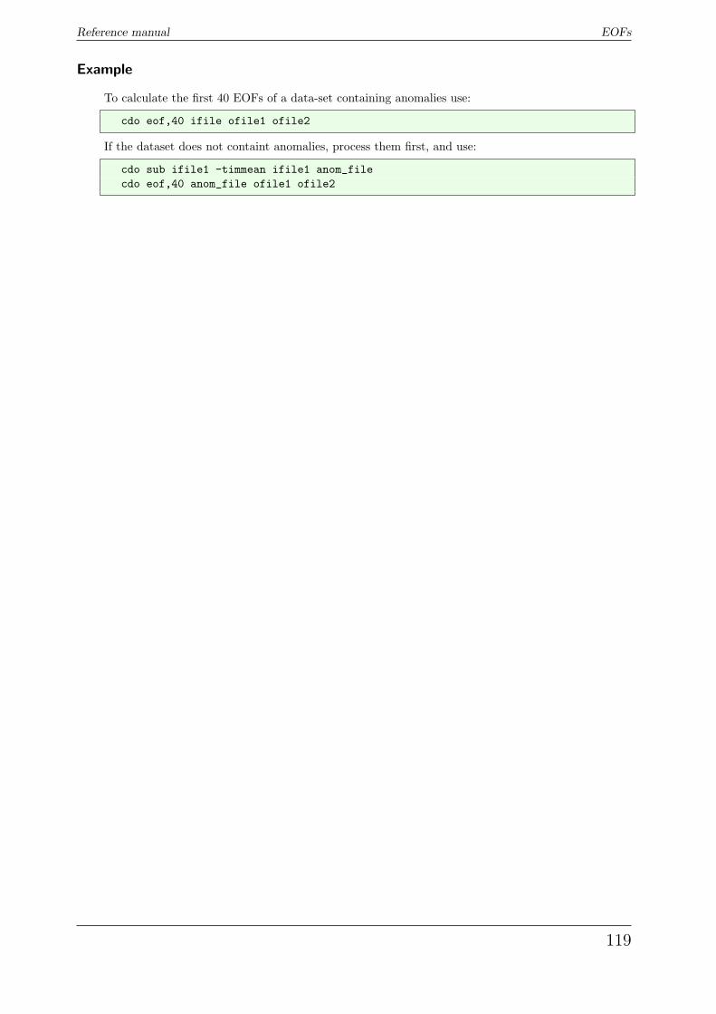
Reference manual EOFs
Example
To calculate the first 40 EOFs of a data-set containing anomalies use:
cdo eof,40 ifile ofile1 ofile2
If the dataset does not containt anomalies, process them first, and use:
cdo sub ifile1 -timmean ifile1 anom_filecdo eof,40 anom_file ofile1 ofile2
119
EOFs Reference manual
2.11.2. EOFCOEFF - Principal coefficients of EOFs
Synopsis
eofcoeff ifile1 ifile2 obase
Description
This module calculates the time series of the principal coefficients for given EOF (empirical orthogonalfunctions) and data. Time steps in ifile1 are assumed to be the EOFs, Time steps in ifile2 areassumed to be the time series. Weights are taken into account, which is why EOF output is notweighted. Note, that this operator calculates a weighted dot product of the fields in ifile1 andifile2. Given a set of EOFs ej and a time series of data z(t) with p entries for each time step fromwhich ej have been calculated, this operator calculates the time series of the projections of data ontoeach EOF
oj(t) =p∑
x=1
W (x, x)z(t, x)ej(x)
where W is the diagonal matrix containing area weights as above. There will be a seperate file oj forthe principal coefficients of each EOF.As the EOFs ej are uncorrelated, so are their principal coefficients, i.e.
n∑t=1
oj(t)ok(t) ={
0 if j 6= k
λj if j = kwith
n∑t=1
oj(t) = 0∀j ∈ {1, . . . , p}.
There will be a separate file containing a time series of principal coefficients with time informationfrom ifile2 for each EOF in ifile1. Output files will be numbered as <obase><neof><suffix>where neof+1 is the number of the EOF (time step) in ifile1 and suffix is the filename extensionderived from the file format.
Environment
CDO FILE SUFFIX This environment variable can be used to set the default file suffix. Thissuffix will be added to the output file names instead of the filename extensionderived from the file format. Set this variable to NULL to disable the addingof a file suffix.
Example
To calculate principal coefficients of the first 40 EOFs of anom file, and write them to files beginningwith obase, use:
cdo eof,40 anom_file eval_file eof_filecdo eofcoeff eof_file anom_file obase
The principal coefficients of the first EOF will be in the file obase000000.nc (and so forth for higherEOFs, nth EOF will be in obase<n-1>).If the dataset ifile does not containt anomalies, process them first, and use:
cdo sub ifile -timmean ifile anom_filecdo eof,40 anom_file eval_file eof_filecdo eofcoeff eof_file anom_file obase
120
Reference manual Interpolation
2.12. Interpolation
This section contains modules to interpolate datasets. There are several operators to interpolate horizontalfields to a new grid. Some of those operators can handle only 2D fields on a regular rectangular grid. Verticalinterpolation of 3D variables is possible from hybrid model levels to height or pressure levels. Interpolationin time is possible between time steps and years.
Here is a short overview of all operators in this section:
remapbil Bilinear interpolationremapbic Bicubic interpolationremapdis Distance-weighted average remappingremapnn Nearest neighbor remappingremapcon First order conservative remappingremapcon2 Second order conservative remappingremaplaf Largest area fraction remapping
genbil Generate bilinear interpolation weightsgenbic Generate bicubic interpolation weightsgendis Generate distance-weighted average remap weightsgennn Generate nearest neighbor remap weightsgencon Generate 1st order conservative remap weightsgencon2 Generate 2nd order conservative remap weightsgenlaf Generate largest area fraction remap weights
remap SCRIP grid remapping
remapeta Remap vertical hybrid level
ml2pl Model to pressure level interpolationml2hl Model to height level interpolation
intlevel Linear level interpolation
inttime Interpolation between time stepsintntime Interpolation between time steps
intyear Interpolation between two years
121
Interpolation Reference manual
2.12.1. REMAPGRID - SCRIP grid interpolation
Synopsis
<operator>,grid ifile ofile
Description
This module contains operators to remap all input fields to a new horizontal grid. Each operator usesa different remapping method. The interpolation is based on an adapted SCRIP library version. Fora detailed description of the remapping methods see [SCRIP].
Operators
remapbil Bilinear interpolationPerforms a bilinear interpolation on all input fields. This interpolation method onlyworks on quadrilateral curvilinear grids.
remapbic Bicubic interpolationPerforms a bicubic interpolation on all input fields. This interpolation method onlyworks on quadrilateral curvilinear grids.
remapdis Distance-weighted average remappingPerforms a distance-weighted average remapping of the four nearest neighbor valueson all input fields.
remapnn Nearest neighbor remappingPerforms a nearest neighbor remapping on all input fields.
remapcon First order conservative remappingPerforms a first order conservative remapping on all input fields.
remapcon2 Second order conservative remappingPerforms a second order conservative remapping on all input fields.
remaplaf Largest area fraction remappingPerforms a largest area fraction remapping on all input fields.
Parameter
grid STRING Target grid description file or name
Environment
NORMALIZE OPT This variable is used to choose the normalization of the conservative remap-ping. By default NORMALIZE OPT is set to ’fracarea’ and will includethe destination area fraction in the output weights; other options are ’none’and ’destarea’ (for more information see [SCRIP]).
REMAP EXTRAPOLATE This variable is used to switch the extrapolation feature ’on’ or ’off’. Bydefault the extrapolation is enabled for remapdis, remapnn and for circulargrids.
Note
For this module the author has converted the original Fortran 90 SCRIP software to ANSI C99. Ifthere are any problems send a bug report to CDO and not to SCRIP!
122
Reference manual Interpolation
Example
Say ifile contains fields on a quadrilateral curvilinear grid. To remap all fields bilinear to a T42Gaussian grid type:
cdo remapbil,t42grid ifile ofile
123
Interpolation Reference manual
2.12.2. GENWEIGHTS - Generate SCRIP grid interpolation weights
Synopsis
<operator>,grid ifile ofile
Description
Interpolation between different horizontal grids can be a very time-consuming process. Especiallyif the data are on an unstructured or a large grid. In this case the SCRIP interpolation processcan be split into two parts. Firstly the generation of the interpolation weights, which is the mosttime-consuming part. These interpolation weights can be reused for every remapping process withthe operator remap. This method should be used only if all input fields are on the same grid and apossibly mask (missing values) does not change. This module contains operators to generate SCRIPinterpolation weights of the first input field. Each operator is using a different interpolation method.
Operators
genbil Generate bilinear interpolation weightsGenerates bilinear interpolation weights and writes the result to a file. This interpola-tion method only works on quadrilateral curvilinear grids.
genbic Generate bicubic interpolation weightsGenerates bicubic interpolation weights and writes the result to a file. This interpolationmethod only works on quadrilateral curvilinear grids.
gendis Generate distance-weighted average remap weightsGenerates distance-weighted average remapping weights of the four nearest neighborvalues and writes the result to a file.
gennn Generate nearest neighbor remap weightsGenerates nearest neighbor remapping weights and writes the result to a file.
gencon Generate 1st order conservative remap weightsGenerates first order conservative remapping weights and writes the result to a file.
gencon2 Generate 2nd order conservative remap weightsGenerates second order conservative remapping weights and writes the result to a file.
genlaf Generate largest area fraction remap weightsGenerates largest area fraction remapping weights and writes the result to a file.
Parameter
grid STRING Target grid description file or name
Environment
NORMALIZE OPT This variable is used to choose the normalization of the conservative in-terpolation. By default NORMALIZE OPT is set to ’fracarea’ and willinclude the destination area fraction in the output weights; other optionsare ’none’ and ’destarea’ (for more information see [SCRIP]).
REMAP EXTRAPOLATE This variable is used to switch the extrapolation feature ’on’ or ’off’. Bydefault the extrapolation is enabled for remapdis, remapnn and for circulargrids.
124
Reference manual Interpolation
Note
For this module the author has converted the original Fortran 90 SCRIP software to ANSI C99. Ifthere are any problems send a bug report to CDO and not to SCRIP!
Example
Say ifile contains fields on a quadrilateral curvilinear grid. To remap all fields bilinear to a T42Gaussian grid use:
cdo genbil,t42grid ifile remapweights.nccdo remap,t42grid,remapweights.nc ifile ofile
125
Interpolation Reference manual
2.12.3. REMAP - SCRIP grid remapping
Synopsis
remap,grid,weights ifile ofile
Description
This operator remaps all input fields to a new horizontal grid. The remap type and the interpolationweights of one input grid are read from a netCDF file. The netCDF file with the weights should followthe SCRIP convention. Normally these weights come from a previous call to module GENWEIGHTSor were created by the original SCRIP package.
Parameter
grid STRING Target grid description file or name
weights STRING Interpolation weights (SCRIP netCDF file)
Environment
NORMALIZE OPT This variable is used to choose the normalization of the conservative in-terpolation. By default NORMALIZE OPT is set to ’fracarea’ and willinclude the destination area fraction in the output weights; other optionsare ’none’ and ’destarea’ (for more information see [SCRIP]).
REMAP EXTRAPOLATE This variable is used to switch the extrapolation feature ’on’ or ’off’. Bydefault the extrapolation is enabled for remapdis, remapnn and for circulargrids.
Note
For this module the author has converted the original Fortran 90 SCRIP software to ANSI C99. Ifthere are any problems send a bug report to CDO and not to SCRIP!
Example
Say ifile contains fields on a quadrilateral curvilinear grid. To remap all fields bilinear to a T42Gaussian grid use:
cdo genbil,t42grid ifile remapweights.nccdo remap,t42grid,remapweights.nc ifile ofile
126
Reference manual Interpolation
2.12.4. REMAPETA - Remap vertical hybrid level
Synopsis
remapeta,vct[,oro] ifile ofile
Description
This operator interpolates between different vertical hybrid levels. This include the preparation ofconsistent data for the free atmosphere. The procedure for the vertical interpolation is based on theHIRLAM scheme and was adapted from [INTERA]. The vertical interpolation is based on the verticalintegration of the hydrostatic equation with few adjustments. The basic tasks are the following one:
� at first integration of hydrostatic equation
� extrapolation of surface pressure
� Planetary Boundary-Layer (PBL) profile interpolation
� interpolation in free atmosphere
� merging of both profiles
� final surface pressure correction
The vertical interpolation corrects the surface pressure. This is simply a cut-off or an addition ofair mass. This mass correction should not influence the geostrophic velocity field in the middletroposhere. Therefore the total mass above a given reference level is conserved. As reference level thegeopotential height of the 500 hPa level is used. Near the surface the correction can affect the verticalstructure of the PBL. Therefore the interpolation is done using the potential temperature. But inthe free atmosphere above a certain n (n=0.8 defining the top of the PBL) the interpolation is donelinearly. After the interpolation both profiles are merged. With the resulting temperature/pressurecorrection the hydrostatic equation is integrated again and adjusted to the reference level finding thefinal surface pressure correction. A more detailed description of the interpolation can be found in[INTERA]. All input fields have to be on the same horizontal grid.
Parameter
vct STRING File name of an ASCII dataset with the vertical coordinate table
oro STRING File name with the orography (surf. geopotential) of the target dataset (optional)
127
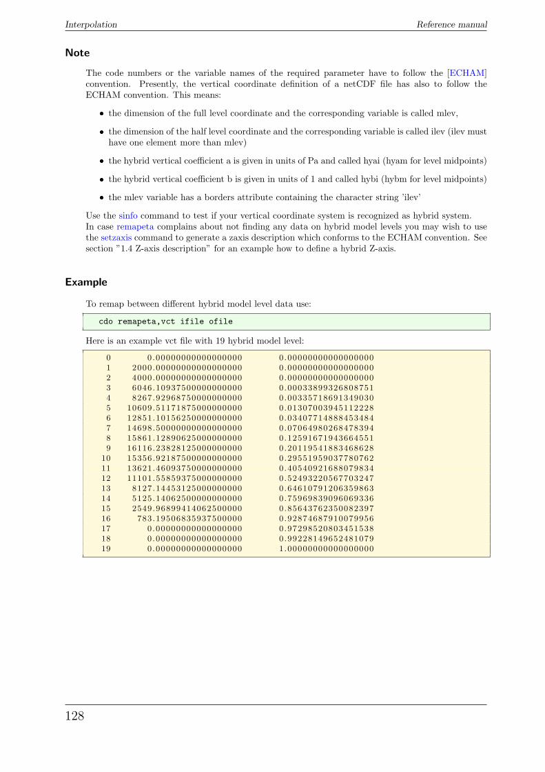
Interpolation Reference manual
Note
The code numbers or the variable names of the required parameter have to follow the [ECHAM]convention. Presently, the vertical coordinate definition of a netCDF file has also to follow theECHAM convention. This means:
� the dimension of the full level coordinate and the corresponding variable is called mlev,
� the dimension of the half level coordinate and the corresponding variable is called ilev (ilev musthave one element more than mlev)
� the hybrid vertical coefficient a is given in units of Pa and called hyai (hyam for level midpoints)
� the hybrid vertical coefficient b is given in units of 1 and called hybi (hybm for level midpoints)
� the mlev variable has a borders attribute containing the character string ’ilev’
Use the sinfo command to test if your vertical coordinate system is recognized as hybrid system.In case remapeta complains about not finding any data on hybrid model levels you may wish to usethe setzaxis command to generate a zaxis description which conforms to the ECHAM convention. Seesection ”1.4 Z-axis description” for an example how to define a hybrid Z-axis.
Example
To remap between different hybrid model level data use:
cdo remapeta,vct ifile ofile
Here is an example vct file with 19 hybrid model level:
0 0.00000000000000000 0.000000000000000001 2000.00000000000000000 0.000000000000000002 4000.00000000000000000 0.000000000000000003 6046.10937500000000000 0.000338993268087514 8267.92968750000000000 0.003357186913490305 10609.51171875000000000 0.013070039451122286 12851.10156250000000000 0.034077148884534847 14698.50000000000000000 0.070649802684783948 15861.12890625000000000 0.125916719436645519 16116.23828125000000000 0.20119541883468628
10 15356.92187500000000000 0.2955195903778076211 13621.46093750000000000 0.4054092168807983412 11101.55859375000000000 0.5249322056770324713 8127.14453125000000000 0.6461079120635986314 5125.14062500000000000 0.7596983909606933615 2549.96899414062500000 0.8564376235008239716 783.19506835937500000 0.9287468791007995617 0.00000000000000000 0.9729852080345153818 0.00000000000000000 0.9922814965248107919 0.00000000000000000 1.00000000000000000
128
Reference manual Interpolation
2.12.5. INTVERT - Vertical interpolation
Synopsis
ml2pl,plevels ifile ofile
ml2hl,hlevels ifile ofile
Description
Interpolate 3D variables on hybrid model levels to pressure or height levels. The input file shouldcontain the log. surface pressure or the surface pressure. To interpolate the temperature, the orogra-phy (surface geopotential) is also needed. The pressure, temperature, and orography are identified bytheir code numbers. Supported parameter tables are: WMO standard table number 2 and ECMWFlocal table number 128. Use the alias ml2plx/ml2hlx or the environment variable EXTRAPOLATE toextrapolate missing values. All input fields have to be on the same horizontal grid.
Operators
ml2pl Model to pressure level interpolationInterpolates 3D variables on hybrid model levels to pressure levels.
ml2hl Model to height level interpolationInterpolates 3D variables on hybrid model levels to height levels. The procedure is thesame as for the operator mh2pl except for the pressure levels being calculated from theheights by: plevel = 101325 ∗ exp(hlevel/− 7000)
Parameter
plevels FLOAT Pressure levels in pascal
hlevels FLOAT Height levels in meter (max level: 65535 m)
Environment
EXTRAPOLATE If set to 1 extrapolate missing values.
Note
The netCDF CF convention for vertical hybrid coordinates is not supported, yet!
Example
To interpolate hybrid model level data to pressure levels of 925, 850, 500 and 200 hPa use:
cdo ml2pl,92500,85000,50000,20000 ifile ofile
129
Interpolation Reference manual
2.12.6. INTLEVEL - Linear level interpolation
Synopsis
intlevel,levels ifile ofile
Description
This operator performs a linear vertical interpolation of non hybrid 3D variables.
Parameter
levels FLOAT Target levels
Example
To interpolate 3D variables on height levels to a new set of height levels use:
cdo intlevel,10,50,100,500,1000 ifile ofile
130
Reference manual Interpolation
2.12.7. INTTIME - Time interpolation
Synopsis
inttime,date,time[,inc] ifile ofile
intntime,n ifile ofile
Description
This module performs linear interpolation between time steps.
Operators
inttime Interpolation between time stepsThis operator creates a new dataset by linear interpolation between time steps. Theuser has to define the start date/time with an optional increment.
intntime Interpolation between time stepsThis operator performs linear interpolation between time steps. The user has to definethe number of time steps from one time step to the next.
Parameter
date STRING Start date (format YYYY-MM-DD)
time STRING Start time (format hh:mm:ss)
inc STRING Optional increment (seconds, minutes, hours, days, months, years) [default:0hour]
n INTEGER Number of time steps from one time step to the next
Example
Assumed a 6 hourly dataset starts at 1987-01-01 12:00. To interpolate this time series to a one hourlydataset use:
cdo inttime,1987-01-01,12:00,1hour ifile ofile
131
Interpolation Reference manual
2.12.8. INTYEAR - Year interpolation
Synopsis
intyear,years ifile1 ifile2 obase
Description
This operator performs linear interpolation between two years, time step by time step. The output fileswill be named <obase><yyyy><suffix> where yyyy will be the year and suffix is the filenameextension derived from the file format.
Parameter
years INTEGER Comma separated list of years
Environment
CDO FILE SUFFIX This environment variable can be used to set the default file suffix. Thissuffix will be added to the output file names instead of the filename extensionderived from the file format. Set this variable to NULL to disable the addingof a file suffix.
Example
Assume there are two monthly mean datasets over a year. The first dataset has 12 time steps forthe year 1985 and the second one for the year 1990. To interpolate the years between 1985 and 1990month by month use:
cdo intyear,1986,1987,1988,1989 ifile1 ifile2 year
Example result of ’dir year*’ for netCDF datasets:
year1986 . nc year1987 . nc year1988 . nc year1989 . nc
132
Reference manual Transformation
2.13. Transformation
This section contains modules to perform spectral transformations.
Here is a short overview of all operators in this section:
sp2gp Spectral to gridpointsp2gpl Spectral to gridpoint (linear)gp2sp Gridpoint to spectralgp2spl Gridpoint to spectral (linear)sp2sp Spectral to spectral
dv2uv Divergence and vorticity to U and V winddv2uvl Divergence and vorticity to U and V wind (linear)uv2dv U and V wind to divergence and vorticityuv2dvl U and V wind to divergence and vorticity (linear)dv2ps D and V to velocity potential and stream function
133
Transformation Reference manual
2.13.1. SPECTRAL - Spectral transformation
Synopsis
sp2gp ifile ofile
sp2gpl ifile ofile
gp2sp ifile ofile
gp2spl ifile ofile
sp2sp,trunc ifile ofile
Description
This module transforms fields on Gaussian grids to spectral coefficients and vice versa.
Operators
sp2gp Spectral to gridpointConvert all fields with spectral coefficients to a regular Gaussian grid. The number oflatitudes of the resulting Gaussian grid is calculated from the triangular truncation by:nlat = NINT ((trunc ∗ 3 + 1.)/2.)
sp2gpl Spectral to gridpoint (linear)Convert all fields with spectral coefficients to a regular Gaussian grid. The number oflatitudes of the resulting Gaussian grid is calculated from the triangular truncation by:nlat = NINT ((trunc ∗ 2 + 1.)/2.)
Use this operator to convert ERA40 data e.g. from TL159 to N80.
gp2sp Gridpoint to spectralConvert all Gaussian gridpoint fields to spectral coefficients. The triangular truncationof the resulting spherical harmonics is calculated from the number of latitudes by:trunc = (nlat ∗ 2− 1)/ 3
gp2spl Gridpoint to spectral (linear)Convert all Gaussian gridpoint fields to spectral coefficients. The triangular truncationof the resulting spherical harmonics is calculated from the number of latitudes by:trunc = (nlat ∗ 2− 1)/ 2
Use this operator to convert ERA40 data e.g. from N80 to TL159 instead of T106.
sp2sp Spectral to spectralChange the triangular truncation of all spectral fields. The operator performs downwardconversion by cutting the resolution. Upward conversions are achieved by filling in zeros.
Parameter
trunc INTEGER New spectral resolution
wnums INTEGER Comma separated list of wave numbers
134
Reference manual Transformation
Example
To transform spectral coefficients from T106 to N80 Gaussian grid use:
cdo sp2gp ifile ofile
To transform spectral coefficients from TL159 to N80 Gaussian grid use:
cdo sp2gpl ifile ofile
135
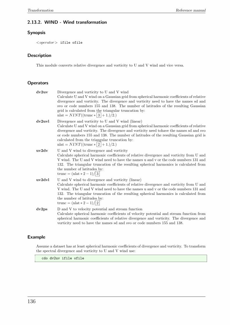
Transformation Reference manual
2.13.2. WIND - Wind transformation
Synopsis
<operator> ifile ofile
Description
This module converts relative divergence and vorticity to U and V wind and vice versa.
Operators
dv2uv Divergence and vorticity to U and V windCalculate U and V wind on a Gaussian grid from spherical harmonic coefficients of relativedivergence and vorticity. The divergence and vorticity need to have the names sd andsvo or code numbers 155 and 138. The number of latitudes of the resulting Gaussiangrid is calculated from the triangular truncation by:nlat = NINT ((trunc ∗ 3 + 1.)/2.)
dv2uvl Divergence and vorticity to U and V wind (linear)Calculate U and V wind on a Gaussian grid from spherical harmonic coefficients of relativedivergence and vorticity. The divergence and vorticity need tohave the names sd and svoor code numbers 155 and 138. The number of latitudes of the resulting Gaussian grid iscalculated from the triangular truncation by:nlat = NINT ((trunc ∗ 2 + 1.)/2.)
uv2dv U and V wind to divergence and vorticityCalculate spherical harmonic coefficients of relative divergence and vorticity from U andV wind. The U and V wind need to have the names u and v or the code numbers 131 and132. The triangular truncation of the resulting spherical harmonics is calculated fromthe number of latitudes by:trunc = (nlat ∗ 2− 1)/ 3
uv2dvl U and V wind to divergence and vorticity (linear)Calculate spherical harmonic coefficients of relative divergence and vorticity from U andV wind. The U and V wind need to have the names u and v or the code numbers 131 and132. The triangular truncation of the resulting spherical harmonics is calculated fromthe number of latitudes by:trunc = (nlat ∗ 2− 1)/ 2
dv2ps D and V to velocity potential and stream functionCalculate spherical harmonic coefficients of velocity potential and stream function fromspherical harmonic coefficients of relative divergence and vorticity. The divergence andvorticity need to have the names sd and svo or code numbers 155 and 138.
Example
Assume a dataset has at least spherical harmonic coefficients of divergence and vorticity. To transformthe spectral divergence and vorticity to U and V wind use:
cdo dv2uv ifile ofile
136
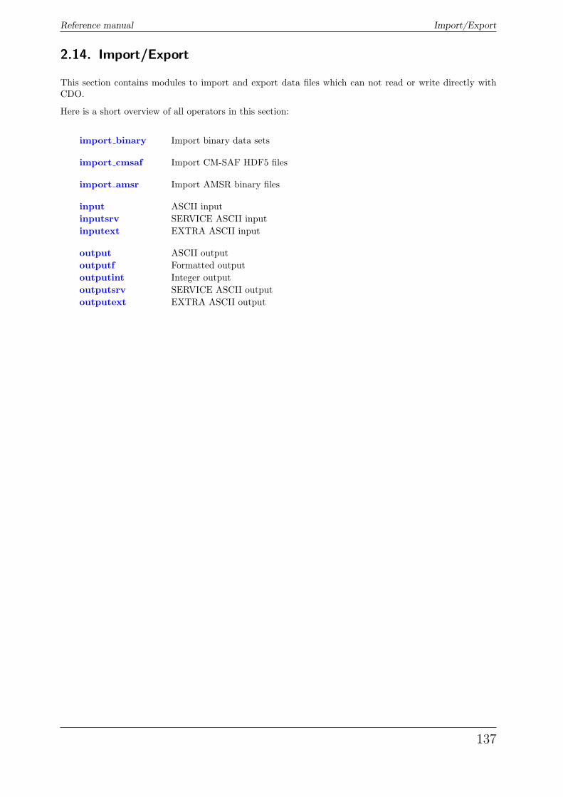
Reference manual Import/Export
2.14. Import/Export
This section contains modules to import and export data files which can not read or write directly withCDO.
Here is a short overview of all operators in this section:
import binary Import binary data sets
import cmsaf Import CM-SAF HDF5 files
import amsr Import AMSR binary files
input ASCII inputinputsrv SERVICE ASCII inputinputext EXTRA ASCII input
output ASCII outputoutputf Formatted outputoutputint Integer outputoutputsrv SERVICE ASCII outputoutputext EXTRA ASCII output
137
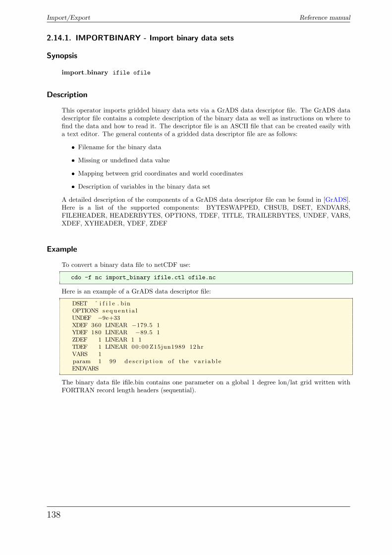
Import/Export Reference manual
2.14.1. IMPORTBINARY - Import binary data sets
Synopsis
import binary ifile ofile
Description
This operator imports gridded binary data sets via a GrADS data descriptor file. The GrADS datadescriptor file contains a complete description of the binary data as well as instructions on where tofind the data and how to read it. The descriptor file is an ASCII file that can be created easily witha text editor. The general contents of a gridded data descriptor file are as follows:
� Filename for the binary data
� Missing or undefined data value
� Mapping between grid coordinates and world coordinates
� Description of variables in the binary data set
A detailed description of the components of a GrADS data descriptor file can be found in [GrADS].Here is a list of the supported components: BYTESWAPPED, CHSUB, DSET, ENDVARS,FILEHEADER, HEADERBYTES, OPTIONS, TDEF, TITLE, TRAILERBYTES, UNDEF, VARS,XDEF, XYHEADER, YDEF, ZDEF
Example
To convert a binary data file to netCDF use:
cdo -f nc import_binary ifile.ctl ofile.nc
Here is an example of a GrADS data descriptor file:
DSET ˆ i f i l e . binOPTIONS s equ en t i a lUNDEF −9e+33XDEF 360 LINEAR −179.5 1YDEF 180 LINEAR −89.5 1ZDEF 1 LINEAR 1 1TDEF 1 LINEAR 00:00 Z15jun1989 12hrVARS 1param 1 99 d e s c r i p t i o n o f the va r i ab l eENDVARS
The binary data file ifile.bin contains one parameter on a global 1 degree lon/lat grid written withFORTRAN record length headers (sequential).
138
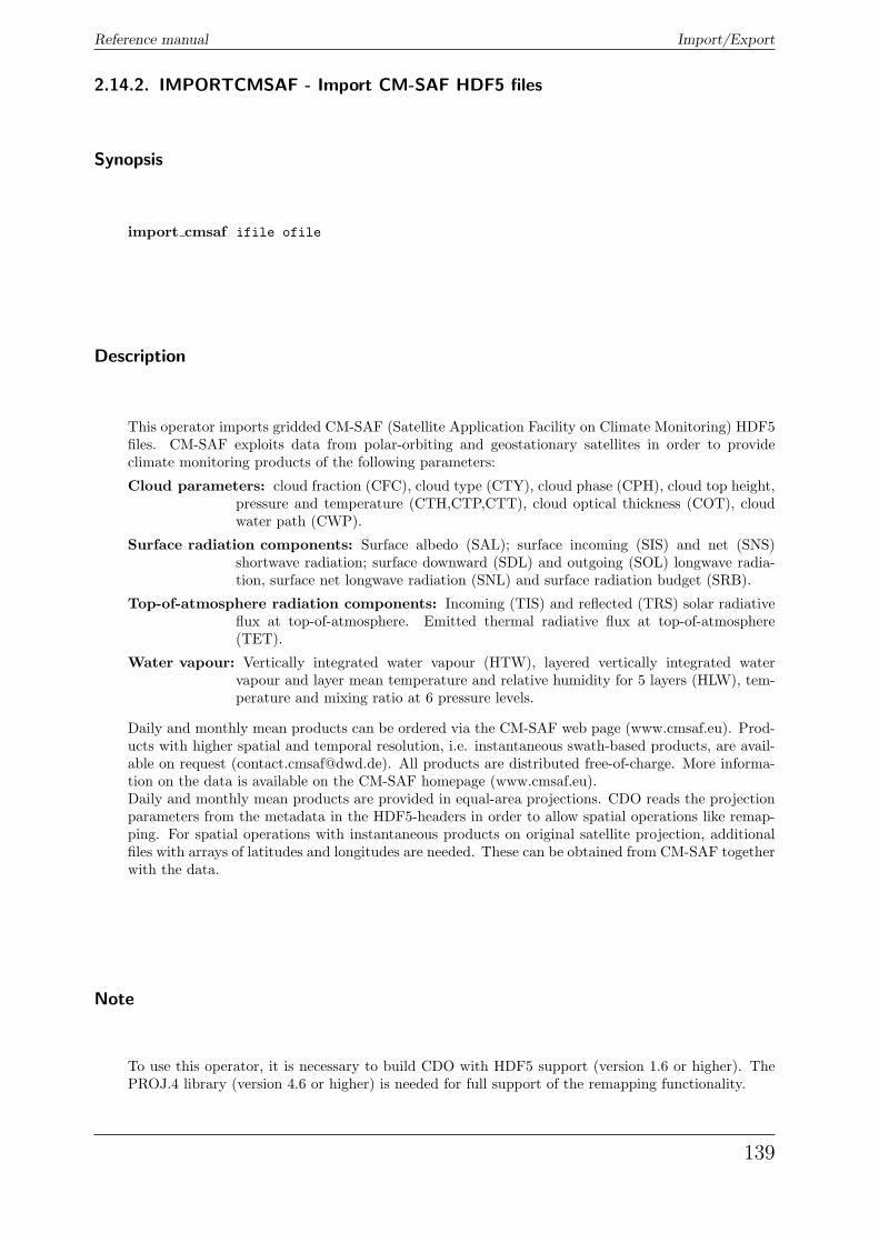
Reference manual Import/Export
2.14.2. IMPORTCMSAF - Import CM-SAF HDF5 files
Synopsis
import cmsaf ifile ofile
Description
This operator imports gridded CM-SAF (Satellite Application Facility on Climate Monitoring) HDF5files. CM-SAF exploits data from polar-orbiting and geostationary satellites in order to provideclimate monitoring products of the following parameters:
Cloud parameters: cloud fraction (CFC), cloud type (CTY), cloud phase (CPH), cloud top height,pressure and temperature (CTH,CTP,CTT), cloud optical thickness (COT), cloudwater path (CWP).
Surface radiation components: Surface albedo (SAL); surface incoming (SIS) and net (SNS)shortwave radiation; surface downward (SDL) and outgoing (SOL) longwave radia-tion, surface net longwave radiation (SNL) and surface radiation budget (SRB).
Top-of-atmosphere radiation components: Incoming (TIS) and reflected (TRS) solar radiativeflux at top-of-atmosphere. Emitted thermal radiative flux at top-of-atmosphere(TET).
Water vapour: Vertically integrated water vapour (HTW), layered vertically integrated watervapour and layer mean temperature and relative humidity for 5 layers (HLW), tem-perature and mixing ratio at 6 pressure levels.
Daily and monthly mean products can be ordered via the CM-SAF web page (www.cmsaf.eu). Prod-ucts with higher spatial and temporal resolution, i.e. instantaneous swath-based products, are avail-able on request ([email protected]). All products are distributed free-of-charge. More informa-tion on the data is available on the CM-SAF homepage (www.cmsaf.eu).Daily and monthly mean products are provided in equal-area projections. CDO reads the projectionparameters from the metadata in the HDF5-headers in order to allow spatial operations like remap-ping. For spatial operations with instantaneous products on original satellite projection, additionalfiles with arrays of latitudes and longitudes are needed. These can be obtained from CM-SAF togetherwith the data.
Note
To use this operator, it is necessary to build CDO with HDF5 support (version 1.6 or higher). ThePROJ.4 library (version 4.6 or higher) is needed for full support of the remapping functionality.
139
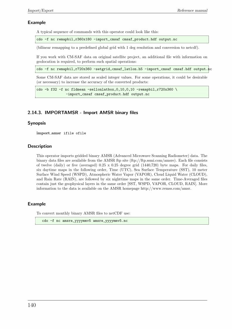
Import/Export Reference manual
Example
A typical sequence of commands with this operator could look like this:
cdo -f nc remapbil,r360x180 -import_cmsaf cmsaf_product.hdf output.nc
(bilinear remapping to a predefined global grid with 1 deg resolution and conversion to netcdf).
If you work with CM-SAF data on original satellite project, an additional file with information ongeolocation is required, to perform such spatial operations:
cdo -f nc remapbil,r720x360 -setgrid,cmsaf_latlon.h5 -import_cmsaf cmsaf.hdf output.nc
Some CM-SAF data are stored as scaled integer values. For some operations, it could be desirable(or necessary) to increase the accuracy of the converted products:
cdo -b f32 -f nc fldmean -sellonlatbox,0,10,0,10 -remapbil,r720x360 \-import_cmsaf cmsaf_product.hdf output.nc
2.14.3. IMPORTAMSR - Import AMSR binary files
Synopsis
import amsr ifile ofile
Description
This operator imports gridded binary AMSR (Advanced Microwave Scanning Radiometer) data. Thebinary data files are available from the AMSR ftp site (ftp://ftp.ssmi.com/amsre). Each file consistsof twelve (daily) or five (averaged) 0.25 x 0.25 degree grid (1440,720) byte maps. For daily files,six daytime maps in the following order, Time (UTC), Sea Surface Temperature (SST), 10 meterSurface Wind Speed (WSPD), Atmospheric Water Vapor (VAPOR), Cloud Liquid Water (CLOUD),and Rain Rate (RAIN), are followed by six nighttime maps in the same order. Time-Averaged filescontain just the geophysical layers in the same order [SST, WSPD, VAPOR, CLOUD, RAIN]. Moreinformation to the data is available on the AMSR homepage http://www.remss.com/amsr.
Example
To convert monthly binary AMSR files to netCDF use:
cdo -f nc amsre_yyyymmv5 amsre_yyyymmv5.nc
140
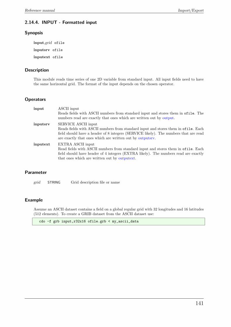
Reference manual Import/Export
2.14.4. INPUT - Formatted input
Synopsis
input,grid ofile
inputsrv ofile
inputext ofile
Description
This module reads time series of one 2D variable from standard input. All input fields need to havethe same horizontal grid. The format of the input depends on the chosen operator.
Operators
input ASCII inputReads fields with ASCII numbers from standard input and stores them in ofile. Thenumbers read are exactly that ones which are written out by output.
inputsrv SERVICE ASCII inputReads fields with ASCII numbers from standard input and stores them in ofile. Eachfield should have a header of 8 integers (SERVICE likely). The numbers that are readare exactly that ones which are written out by outputsrv.
inputext EXTRA ASCII inputRead fields with ASCII numbers from standard input and stores them in ofile. Eachfield should have header of 4 integers (EXTRA likely). The numbers read are exactlythat ones which are written out by outputext.
Parameter
grid STRING Grid description file or name
Example
Assume an ASCII dataset contains a field on a global regular grid with 32 longitudes and 16 latitudes(512 elements). To create a GRIB dataset from the ASCII dataset use:
cdo -f grb input,r32x16 ofile.grb < my_ascii_data
141
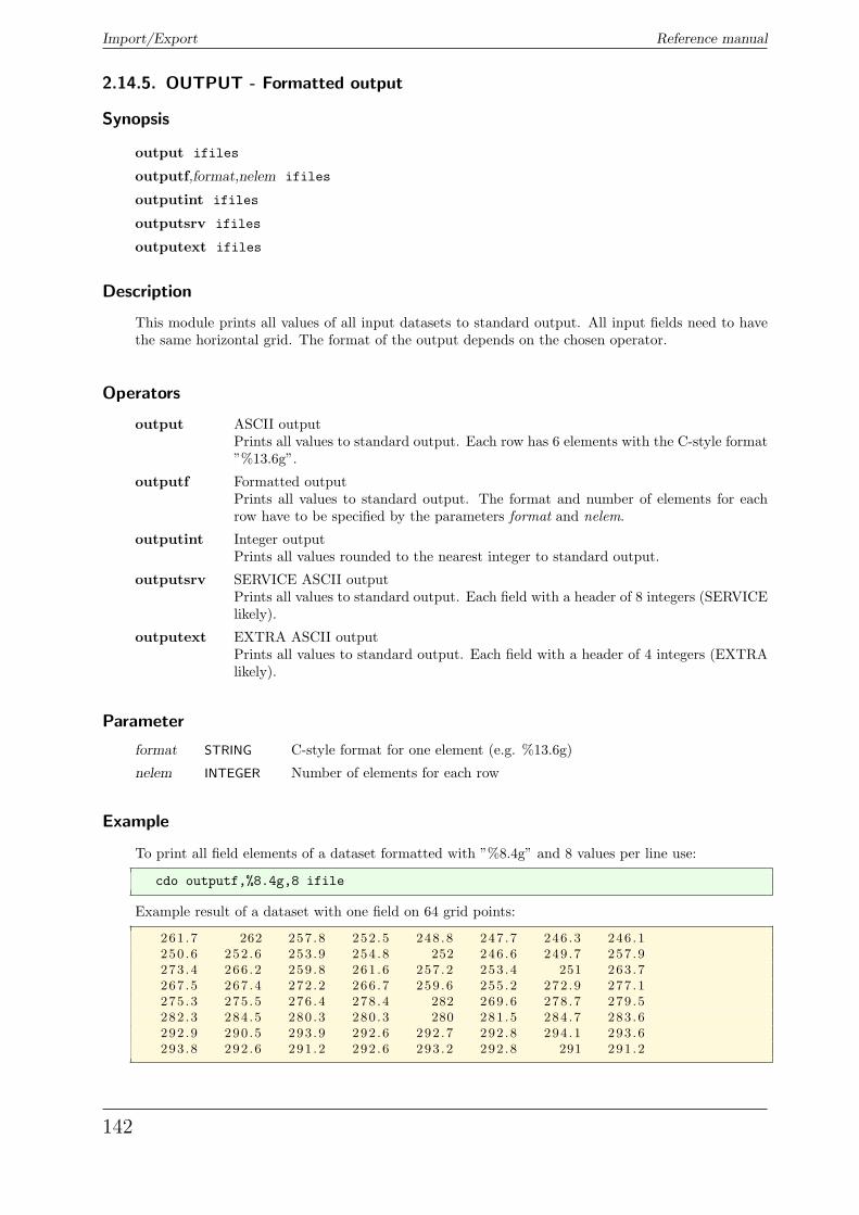
Import/Export Reference manual
2.14.5. OUTPUT - Formatted output
Synopsis
output ifiles
outputf,format,nelem ifiles
outputint ifiles
outputsrv ifiles
outputext ifiles
Description
This module prints all values of all input datasets to standard output. All input fields need to havethe same horizontal grid. The format of the output depends on the chosen operator.
Operators
output ASCII outputPrints all values to standard output. Each row has 6 elements with the C-style format”%13.6g”.
outputf Formatted outputPrints all values to standard output. The format and number of elements for eachrow have to be specified by the parameters format and nelem.
outputint Integer outputPrints all values rounded to the nearest integer to standard output.
outputsrv SERVICE ASCII outputPrints all values to standard output. Each field with a header of 8 integers (SERVICElikely).
outputext EXTRA ASCII outputPrints all values to standard output. Each field with a header of 4 integers (EXTRAlikely).
Parameter
format STRING C-style format for one element (e.g. %13.6g)
nelem INTEGER Number of elements for each row
Example
To print all field elements of a dataset formatted with ”%8.4g” and 8 values per line use:
cdo outputf,%8.4g,8 ifile
Example result of a dataset with one field on 64 grid points:
261 .7 262 257 .8 252 .5 248 .8 247 .7 246 .3 246 .1250 .6 252 .6 253 .9 254 .8 252 246 .6 249 .7 257 .9273 .4 266 .2 259 .8 261 .6 257 .2 253 .4 251 263 .7267 .5 267 .4 272 .2 266 .7 259 .6 255 .2 272 .9 277 .1275 .3 275 .5 276 .4 278 .4 282 269 .6 278 .7 279 .5282 .3 284 .5 280 .3 280 .3 280 281 .5 284 .7 283 .6292 .9 290 .5 293 .9 292 .6 292 .7 292 .8 294 .1 293 .6293 .8 292 .6 291 .2 292 .6 293 .2 292 .8 291 291 .2
142
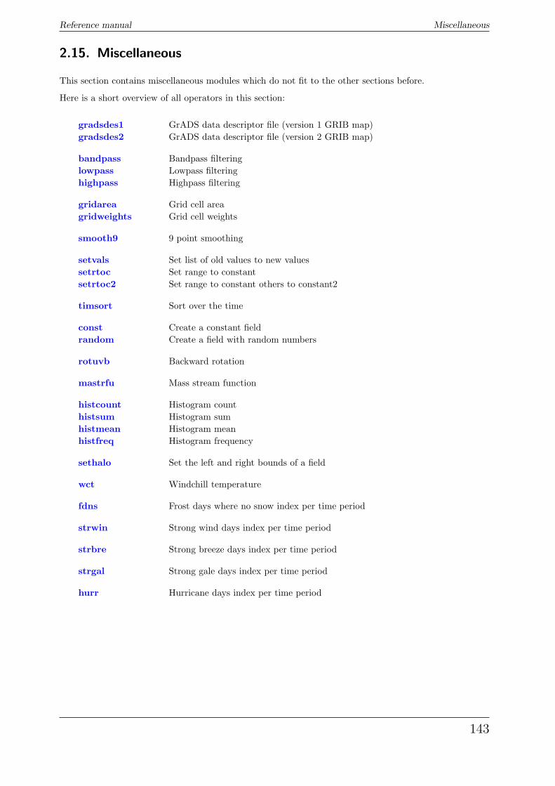
Reference manual Miscellaneous
2.15. Miscellaneous
This section contains miscellaneous modules which do not fit to the other sections before.
Here is a short overview of all operators in this section:
gradsdes1 GrADS data descriptor file (version 1 GRIB map)gradsdes2 GrADS data descriptor file (version 2 GRIB map)
bandpass Bandpass filteringlowpass Lowpass filteringhighpass Highpass filtering
gridarea Grid cell areagridweights Grid cell weights
smooth9 9 point smoothing
setvals Set list of old values to new valuessetrtoc Set range to constantsetrtoc2 Set range to constant others to constant2
timsort Sort over the time
const Create a constant fieldrandom Create a field with random numbers
rotuvb Backward rotation
mastrfu Mass stream function
histcount Histogram counthistsum Histogram sumhistmean Histogram meanhistfreq Histogram frequency
sethalo Set the left and right bounds of a field
wct Windchill temperature
fdns Frost days where no snow index per time period
strwin Strong wind days index per time period
strbre Strong breeze days index per time period
strgal Strong gale days index per time period
hurr Hurricane days index per time period
143
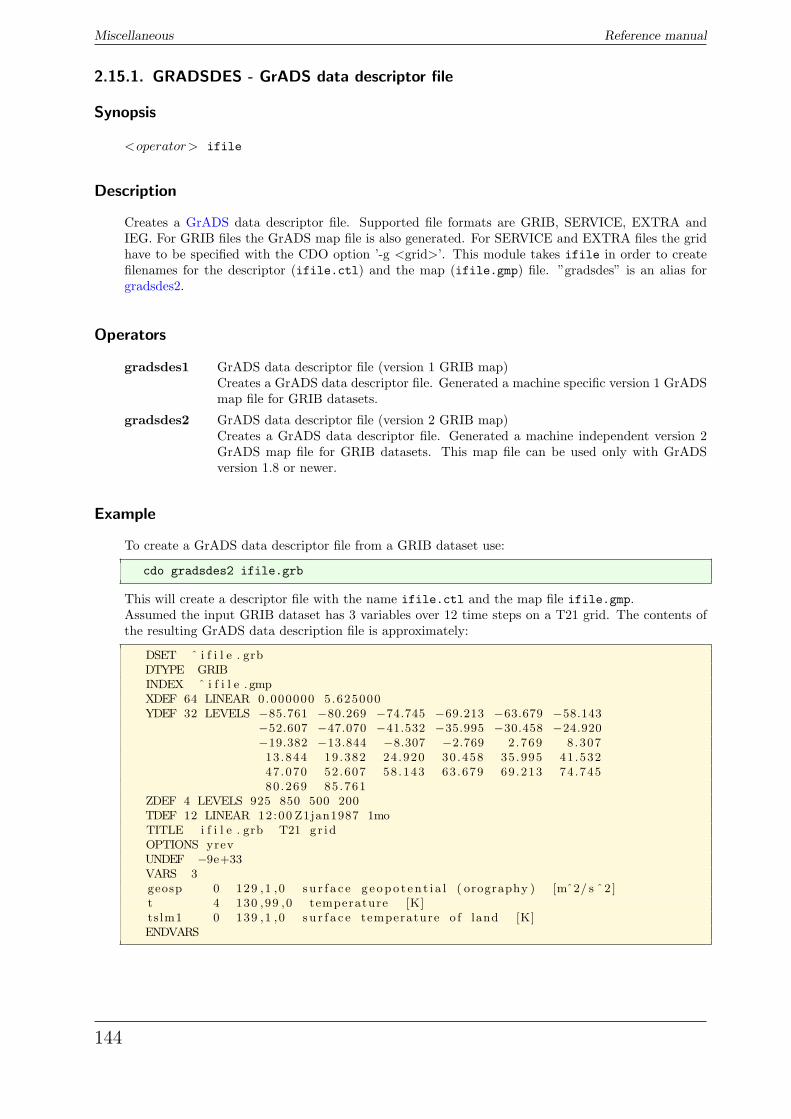
Miscellaneous Reference manual
2.15.1. GRADSDES - GrADS data descriptor file
Synopsis
<operator> ifile
Description
Creates a GrADS data descriptor file. Supported file formats are GRIB, SERVICE, EXTRA andIEG. For GRIB files the GrADS map file is also generated. For SERVICE and EXTRA files the gridhave to be specified with the CDO option ’-g <grid>’. This module takes ifile in order to createfilenames for the descriptor (ifile.ctl) and the map (ifile.gmp) file. ”gradsdes” is an alias forgradsdes2.
Operators
gradsdes1 GrADS data descriptor file (version 1 GRIB map)Creates a GrADS data descriptor file. Generated a machine specific version 1 GrADSmap file for GRIB datasets.
gradsdes2 GrADS data descriptor file (version 2 GRIB map)Creates a GrADS data descriptor file. Generated a machine independent version 2GrADS map file for GRIB datasets. This map file can be used only with GrADSversion 1.8 or newer.
Example
To create a GrADS data descriptor file from a GRIB dataset use:
cdo gradsdes2 ifile.grb
This will create a descriptor file with the name ifile.ctl and the map file ifile.gmp.Assumed the input GRIB dataset has 3 variables over 12 time steps on a T21 grid. The contents ofthe resulting GrADS data description file is approximately:
DSET ˆ i f i l e . grbDTYPE GRIBINDEX ˆ i f i l e . gmpXDEF 64 LINEAR 0.000000 5.625000YDEF 32 LEVELS −85.761 −80.269 −74.745 −69.213 −63.679 −58.143
−52.607 −47.070 −41.532 −35.995 −30.458 −24.920−19.382 −13.844 −8.307 −2.769 2 .769 8 .30713 .844 19 .382 24 .920 30 .458 35 .995 41 .53247 .070 52 .607 58 .143 63 .679 69 .213 74 .74580 .269 85 .761
ZDEF 4 LEVELS 925 850 500 200TDEF 12 LINEAR 12:00 Z1jan1987 1moTITLE i f i l e . grb T21 gr idOPTIONS yrevUNDEF −9e+33VARS 3geosp 0 129 ,1 ,0 s u r f a c e g eopo t en t i a l ( orography ) [mˆ2/ s ˆ2 ]t 4 130 ,99 ,0 temperature [K]ts lm1 0 139 ,1 ,0 s u r f a c e temperature o f land [K]ENDVARS
144
Reference manual Miscellaneous
2.15.2. FILTER - Time series filtering
Synopsis
bandpass,fmin,fmax ifile ofile
lowpass,fmax ifile ofile
highpass,fmin ifile ofile
Description
This module takes the time series for each gridpoint in ifile and fills it with zeros (zero- padding)up to the next time-step-number that is a power of 2. Then it (fast fourier) transforms the time serieswith 2n elements into the frequency domain. According to the particular operator and its parameterscertain frequencies are filtered (set to zero) in the frequency domain and the spectrum is (inverse fastfourier) transformed back into the time domain. This time series is cut to the original number oftimesteps from ifile and written to ofile. To determine the frequency the time-axis of ifile isused. (Data should have a constant time increment since this assumption applies for transformation.However, the time increment has to be different from zero.) All frequencies given as parameter areinterpreted per year. This is done by the assumption of a 365-day calendar. Consequently if youwant to perform multiyear-filtering accurately you have to delete the 29th of February. If your ifilehas a 360 year calendar the frequency parameters fmin respectively fmax should be multiplied with afactor of 360/365 in order to obtain accurate results. For the set up of a frequency filter the frequencyparameters have to be adjusted to a frequency in the data. Here fmin is rounded down and fmax isalways rounded up. Consequently it is possible to use bandpass with fmin=fmax without getting azero-field for ofile. Hints for efficient usage:
� to avoid effects of zero-padding cut or extend your time series down/up to the nearest power oftwo
� to get reliable results the time-series has to be detrended (cdo detrend)
� the lowest frequency greater zero that can be contained in ifile is 1/(N*dT),
� the greatest frequency is 1/(2dT) (Nyquist frequency),
with N the number of time steps and dT the time increment of ifile in years.
Operators
bandpass Bandpass filteringBandpass filtering (pass for frequencies between fmin and fmax). Suppresses all vari-ability outside the frequency range specified by [fmin,fmax].
lowpass Lowpass filteringLowpass filtering (pass for frequencies lower than fmax). Suppresses all variabilitywith frequencies greater than fmax.
highpass Highpass filteringHighpass filtering (pass for frequencies greater than fmin). Suppresses all variabiltywith frequencies lower than fmin.
Parameter
fmin FLOAT Minimum frequency per year that passes the filter.
fmax FLOAT Maximum frequency per year that passes the filter.
145
Miscellaneous Reference manual
Example
Now assume your data are still hourly for a time period of 5 years but with a 365/366-day- calendarand you want to suppress the variability on timescales greater ore equal to one year (we suggest hereto use a number x bigger than one (e.g. x=1.5) since there will be dominant frequencies around thepeak (if there is one) as well due to the issue that the time series is not of infinite length). Thereforyou can use the following:
cdo highpass,x -del29feb ifile ofile
Accordingly you might use the following to suppress variability on timescales shorter than one year:
cdo lowpass,1 -del29feb ifile ofile
Finally you might be interested in 2-year variability. If you want to suppress the seasonal cycle aswell as say the longer cycles in climate system you might use
cdo bandpass,x,y -del29feb ifile ofile
with x<=0.5 and y >=0.5.
2.15.3. GRIDCELL - Grid cell quantities
Synopsis
<operator> ifile ofile
Description
This module reads the grid cell area of the first grid from the input stream. If the grid cell area ismissing it will be computed from the grid description. Depending on the chosen operator the gridcell area or weights are written to the output stream.
Operators
gridarea Grid cell areaWrites the grid cell area to the output stream. If the grid cell area have to becomputed it is scaled with the earth radius to square meters.
gridweights Grid cell weightsWrites the grid cell area weights to the output stream.
Environment
PLANET RADIUS This variable is used to scale the computed grid cell areas to square meters. Bydefault PLANET RADIUS is set to an earth radius of 6371000 meter.
146
Reference manual Miscellaneous
2.15.4. SMOOTH9 - 9 point smoothing
Synopsis
smooth9 ifile ofile
Description
Performs a 9 point smoothing on all fields with a quadrilateral curvilinear grid. The result at eachgrid point is a weighted average of the grid point plus the 8 surrounding points. The center pointreceives a weight of 1.0, the points at each side and above and below receive a weight of 0.5, andcorner points receive a weight of 0.3. All 9 points are multiplied by their weights and summed, thendivided by the total weight to obtain the smoothed value. Any missing data points are not includedin the sum; points beyond the grid boundary are considered to be missing. Thus the final result maybe the result of an averaging with less than 9 points.
2.15.5. REPLACEVALUES - Replace variable values
Synopsis
setvals,oldval,newval[,...] ifile ofile
setrtoc,rmin,rmax,c ifile ofile
setrtoc2,rmin,rmax,c,c2 ifile ofile
Description
This module replaces old variable values with new values, depending on the operator.
Operators
setvals Set list of old values to new valuesSupply a list of n pairs of old and new values.
setrtoc Set range to constant
o(t, x) ={
c if i(t, x) ≥ rmin ∧ i(t, x) ≤ rmax
i(t, x) if i(t, x) < rmin ∨ i(t, x) > rmax
setrtoc2 Set range to constant others to constant2
o(t, x) ={
c if i(t, x) ≥ rmin ∧ i(t, x) ≤ rmax
c2 if i(t, x) < rmin ∨ i(t, x) > rmax
Parameter
oldval,newval,... FLOAT Pairs of old and new values
rmin FLOAT Lower bound
rmax FLOAT Upper bound
c FLOAT New value - inside range
c2 FLOAT New value - outside range
147
Miscellaneous Reference manual
2.15.6. TIMSORT - Timsort
Synopsis
timsort ifile ofile
Description
Sorts the elements in ascending order over all time steps for every field position. After sorting it is:
o(t1, x) <= o(t2, x) ∀(t1 < t2), x
Example
To sort all field elements of a dataset over all time steps use:
cdo timsort ifile ofile
2.15.7. VARGEN - Generate a field
Synopsis
const,const,grid ofile
random,grid[,seed] ofile
Description
Generates a dataset with one field. The size of the field is specified by the user given grid description.According to the chosen operator all field elements are constant or filled with random numbers.
Operators
const Create a constant fieldCreates a constant field. All field elements of the grid have the same value.
random Create a field with random numbersCreates a field with rectangularly distrubuted random numbers in the interval [0,1].
Parameter
const FLOAT Constant
seed INTEGER The seed for a new sequence of pseudo-random numbers [default: 1]
grid STRING Target grid description file or name
148
Reference manual Miscellaneous
2.15.8. ROTUV - Rotation
Synopsis
rotuvb,u,v,... ifile ofile
Description
This is a special operator for datsets with wind components on a rotated grid, e.g. data from theregional model REMO. It performs a backward transformation of velocity components U and V froma rotated spherical system to a geographical system.
Parameter
u,v,... STRING Pairs of zonal and meridional velocity components (use variable names orcode numbers)
Example
To transform the u and v velocity of a dataset from a rotated spherical system to a geographicalsystem use:
cdo rotuvb,u,v ifile ofile
2.15.9. MASTRFU - Mass stream function
Synopsis
mastrfu ifile ofile
Description
This is a special operator for the post processing of the atmospheric general circulation modelECHAM. It computes the mass stream function (code number 272). The input dataset have tobe a zonal mean of v-velocity (code number 132) on pressure levels.
Example
To compute the mass stream function from a zonal mean v-velocity dataset use:
cdo mastrfu ifile ofile
149
Miscellaneous Reference manual
2.15.10. HISTOGRAM - Histogram
Synopsis
<operator>,bounds ifile ofile
Description
This module creates bins for a histogram of the input data. The bins have to be adjacent and havenon-overlapping intervals. The user has to define the bounds of the bins. The first value is the lowerbound and the second value the upper bound of the first bin. The bounds of the second bin aredefined by the second and third value, aso. Only 2-dimensional input fields are allowed. The ouputfile contains one vertical level for each of the bins requested.
Operators
histcount Histogram countNumber of elements in the bin range.
histsum Histogram sumSum of elements in the bin range.
histmean Histogram meanMean of elements in the bin range.
histfreq Histogram frequencyRelative frequency of elements in the bin range.
Parameter
bounds FLOAT Comma separated list of the bin bounds (-inf and inf valid)
2.15.11. SETHALO - Set the left and right bounds of a field
Synopsis
sethalo,lhalo,rhalo ifile ofile
Description
This operator sets the left and right bounds of the rectangularly understood fields. Positive numbersof the parameter lhalo enlarges the left bound by the given number of columns from the right bound.The parameter rhalo does the similar for the right bound. Negative numbers of the parameterlhalo/rhalo can be used to remove the given number of columns of the left and right bounds.
Parameter
lhalo INTEGER Left halo
rhalo INTEGER Right halo
150
Reference manual Miscellaneous
2.15.12. WCT - Windchill temperature
Synopsis
wct ifile1 ifile2 ofile
Description
Let ifile1 and ifile2 be time series of temperature and wind speed records, then a correspondingtime series of resulting windchill temperatures is written to ofile. The wind chill temperature calcu-lation is only valid for a temperature of T <= 33 � and a wind speed of v >= 1.39 m/s. Wheneverthese conditions are not satisfied, a missing value is written to ofile. Note that temperature andwind speed records have to be given in units of � and m/s, respectively.
2.15.13. FDNS - Frost days where no snow index per time period
Synopsis
fdns ifile1 ifile2 ofile
Description
Let ifile1 be a time series of daily minimum temperatures TN and ifile2 be a corresponding seriesof daily surface snow amounts. Then counted is the number of days where TN < 0 � and the surfacesnow amount is less than 1 cm. The temperature TN have to be given in units of Kelvin. The dateinformation of a time step in ofile is the date of the last contributing time step in ifile.
2.15.14. STRWIN - Strong wind days index per time period
Synopsis
strwin[,v] ifile ofile
Description
Let ifile be a time series of daily maximum horizontal wind speeds VX, then counted is the numberof days where VX > v. The horizontal wind speed v is an optional parameter with default v = 10.5m/s. A further output variable is the maximum number of consecutive days with maximum windspeed greater than or equal to v. Note that both VX and v have to be given in units of m/s. Alsonote that the horizontal wind speed is defined as the square root of the sum of squares of the zonaland meridional wind speeds. The date information of a time step in ofile is the date of the lastcontributing time step in ifile.
Parameter
v FLOAT Horizontal wind speed threshold (m/s, default v = 10.5 m/s)
151
Miscellaneous Reference manual
2.15.15. STRBRE - Strong breeze days index per time period
Synopsis
strbre ifile ofile
Description
Let ifile be a time series of daily maximum horizontal wind speeds VX, then counted is the numberof days where VX is greater than or equal to 10.5 m/s. A further output variable is the maximumnumber of consecutive days with maximum wind speed greater than or equal to 10.5 m/s. Note thatVX is defined as the square root of the sum of squares of the zonal and meridional wind speeds andhave to be given in units of m/s. The date information of a time step in ofile is the date of the lastcontributing time step in ifile.
2.15.16. STRGAL - Strong gale days index per time period
Synopsis
strgal ifile ofile
Description
Let ifile be a time series of daily maximum horizontal wind speeds VX, then counted is the numberof days where VX is greater than or equal to 20.5 m/s. A further output variable is the maximumnumber of consecutive days with maximum wind speed greater than or equal to 20.5 m/s. Note thatVX is defined as the square root of the sum of square of the zonal and meridional wind speeds andhave to be given in units of m/s. The date information of a time step in ofile is the date of the lastcontributing time step in ifile.
2.15.17. HURR - Hurricane days index per time period
Synopsis
hurr ifile ofile
Description
Let ifile be a time series of daily maximum horizontal wind speeds VX, then counted is the numberof days where VX is greater than or equal to 32.5 m/s. A further output variable is the maximumnumber of consecutive days with maximum wind speed greater than or equal to 32.5 m/s. Note thatVX is defined as the square root of the sum of squares of the zonal and meridional wind speeds andhave to be given in units of m/s. The date information of a time step in ofile is the date of the lastcontributing time step in ifile.
152
Reference manual Climate indices
2.16. Climate indices
This section contains modules to compute the climate indices of daily temperature and precipitationextremes.
Here is a short overview of all operators in this section:
eca cdd Consecutive dry days index per time period
eca cfd Consecutive frost days index per time period
eca csu Consecutive summer days index per time period
eca cwd Consecutive wet days index per time period
eca cwdi Cold wave duration index wrt mean of reference period
eca cwfi Cold-spell days index wrt 10th percentile of reference period
eca etr Intra-period extreme temperature range
eca fd Frost days index per time period
eca gsl Growing season length index
eca hd Heating degree days per time period
eca hwdi Heat wave duration index wrt mean of reference period
eca hwfi Warm spell days index wrt 90th percentile of reference period
eca id Ice days index per time period
eca pd Precipitation days index per time periodeca r10mm Heavy precipitation days index per time periodeca r20mm Very heavy precipitation days index per time period
eca r75p Moderate wet days wrt 75th percentile of reference period
eca r75ptot Precipitation percent due to R75p days
eca r90p Wet days wrt 90th percentile of reference period
eca r90ptot Precipitation percent due to R90p days
eca r95p Very wet days wrt 95th percentile of reference period
eca r95ptot Precipitation percent due to R95p days
eca r99p Extremely wet days wrt 99th percentile of reference period
eca r99ptot Precipitation percent due to R99p days
eca rr1 Wet days index per time period
eca rx1day Highest one day precipitation amount per time period
eca rx5day Highest five-day precipitation amount per time period
153
Climate indices Reference manual
eca sdii Simple daily intensity index per time period
eca su Summer days index per time period
eca tg10p Cold days percent wrt 10th percentile of reference period
eca tg90p Warm days percent wrt 90th percentile of reference period
eca tn10p Cold nights percent wrt 10th percentile of reference period
eca tn90p Warm nights percent wrt 90th percentile of reference period
eca tr Tropical nights index per time period
eca tx10p Very cold days percent wrt 10th percentile of reference period
eca tx90p Very warm days percent wrt 90th percentile of reference period
154
Reference manual Climate indices
2.16.1. ECACDD - Consecutive dry days index per time period
Synopsis
eca cdd ifile ofile
Description
Let ifile be a time series of daily precipitation amounts RR, then counted is the largest number ofconsecutive days where RR is less than 1 mm. A further output variable is the number of dry periodsof more than 5 days. The date information of a time step in ofile is the date of the last contributingtime step in ifile. The following variables are created:
� consecutive dry days index per time period
� number of cdd periods with more than 5days per time period
Example
To get the largest number of consecutive dry days of a time series of daily precipitation amounts use:
cdo eca_cdd rrfile ofile
2.16.2. ECACFD - Consecutive frost days index per time period
Synopsis
eca cfd ifile ofile
Description
Let ifile be a time series of daily minimum temperatures TN, then counted is the largest numberof consecutive days where TN < 0 �. Note that TN have to be given in units of Kelvin. The dateinformation of a time step in ofile is the date of the last contributing time step in ifile. Thefollowing variables are created:
� consecutive frost days index per time period
Example
To get the largest number of consecutive frost days of a time series of daily minimum temperaturesuse:
cdo eca_cfd tnfile ofile
155
Climate indices Reference manual
2.16.3. ECACSU - Consecutive summer days index per time period
Synopsis
eca csu[,T] ifile ofile
Description
Let ifile be a time series of daily maximum temperatures TX, then counted is the largest numberof consecutive days where TX > T. The number T is an optional parameter with default T = 25 �.Note that TN have to be given in units of Kelvin, whereas T have to be given in degrees Celsius. Thedate information of a time step in ofile is the date of the last contributing time step in ifile. Thefollowing variables are created:
� consecutive summer days index per time period
Parameter
T FLOAT Temperature threshold ( Celsius, default: T = 25 Celsius)
Example
To get the largest number of consecutive summer days of a time series of daily minimum temperaturesuse:
cdo eca_csu txfile ofile
2.16.4. ECACWD - Consecutive wet days index per time period
Synopsis
eca cwd ifile ofile
Description
Let ifile be a time series of daily precipitation amounts RR, then counted is the largest number ofconsecutive days where RR is at least 1 mm. A further output variable is the number of wet periodsof more than 5 days. The date information of a time step in ofile is the date of the last contributingtime step in ifile. The following variables are created:
� consecutive wet days index per time period
� number of cwd periods with more than 5days per time period
Example
To get the largest number of consecutive wet days of a time series of daily precipitation amounts use:
cdo eca_cwd rrfile ofile
156
Reference manual Climate indices
2.16.5. ECACWDI - Cold wave duration index wrt mean of reference period
Synopsis
eca cwdi[,nday[,T]] ifile1 ifile2 ofile
Description
Let ifile1 be a time series of daily minimum temperatures TN, and let ifile2 be the mean TNnormof daily minimum temperatures for any period used as reference. Then counted is the number of dayswhere, in intervals of at least nday consecutive days, TN < TNnorm - T. The numbers nday and Tare optional parameters with default nday = 6 and T = 5 �. A further output variable is the numberof cold waves longer than or equal to nday days. Note that both TN and TNnorm have to be givenin the same units. The date information of a time step in ofile is the date of the last contributingtime step in ifile1. The following variables are created:
� cold wave duration index wrt mean of reference period
� cold waves per time period
Parameter
nday INTEGER Number of consecutive days (default: nday = 6)
T FLOAT Temperature offset ( Celsius, default: T = 5 Celsius)
Example
To compute the cold wave duration index of a time series of daily minimum temperatures use:
cdo eca_cwdi tnfile tnnormfile ofile
2.16.6. ECACWFI - Cold-spell days index wrt 10th percentile of reference period
Synopsis
eca cwfi[,nday] ifile1 ifile2 ofile
Description
Let ifile1 be a time series of daily mean temperatures TG, and ifile2 be the 10th percentile TGn10of daily mean temperatures for any period used as reference. Then counted is the number of dayswhere, in intervals of at least nday consecutive days, TG < TGn10. The number nday is an optionalparameter with default nday = 6. A further output variable is the number of cold-spell periods longerthan or equal to nday days. Note that both TG and TGn10 have to be given in the same units. Thedate information of a time step in ofile is the date of the last contributing time step in ifile1. Thefollowing variables are created:
� cold spell days index wrt 10th percentile of reference period
� cold spell periods per time period
157

Climate indices Reference manual
Parameter
nday INTEGER Number of consecutive days (default: nday = 6)
Example
To compute the number of cold-spell days of a time series of daily mean temperatures use:
cdo eca_cwfi tgfile tgn10file ofile
158
Reference manual Climate indices
2.16.7. ECAETR - Intra-period extreme temperature range
Synopsis
eca etr ifile1 ifile2 ofile
Description
Let ifile1 and ifile2 be time series of maximum and minimum temperatures TX and TN, respec-tively. Then the extreme temperature range is the difference of the maximum of TX and the minimumof TN. Note that TX and TN have to be given in the same units. The date information of a timestep in ofile is the date of the last contributing time steps in ifile1 and ifile2. The followingvariables are created:
� intra period extreme temperature range
Example
To get the intra-period extreme temperature range for two time series of maximum and minimumtemperatures use:
cdo eca_etr txfile tnfile ofile
2.16.8. ECAFD - Frost days index per time period
Synopsis
eca fd ifile ofile
Description
Let ifile be a time series of daily minimum temperatures TN, then counted is the number of dayswhere TN < 0 �. Note that TN have to be given in units of Kelvin. The date information of a timestep in ofile is the date of the last contributing time step in ifile. The following variables arecreated:
� frost days index per time period
Example
To get the number of frost days of a time series of daily minimum temperatures use:
cdo eca_fd tnfile ofile
159
Climate indices Reference manual
2.16.9. ECAGSL - Thermal Growing season length index
Synopsis
eca gsl[,nday[,T[,fland]]] ifile1 ifile2 ofile
Description
Let ifile1 be a time series of daily mean temperatures TG, and ifile2 be a land-water mask.Within a period of 12 months, the thermal growing season length is officially defined as the numberof days between:
� frist occurrence of at least nday consecutive days with TG > T
� first occurrence of at least nday consecutive days with TG < T within the last 6 months
On northern hemispere, this period corresponds with the regular year, whereas on southern hemispere,it starts at july 1st. Please note, that this definition may lead to weird results concerning values TG= T: In the first half of the period, these days do not contribute to the gsl, but they do within thesecond half. Moreover this definition could lead to discontinuous values in equatorial regions.The numbers nday and T are optional parameter with default nday = 6 and T = 5 �. The numberfland is an optional parameter with default value fland = 0.5 and denotes the fraction of a grid pointthat have to be covered by land in order to be included in the calculation. A further output variableis the start day of year of the growing season. Note that TG have to be given in units of Kelvin,whereas T have to be given in degrees Celsius.The date information of a time step in ofile is the date of the last contributing time step in ifile.The following variables are created:
� thermal growing season length
� day of year of growing season start
Parameter
nday INTEGER Number of consecutive days (default: nday = 6)
T FLOAT Temperature threshold (degree Celsius, default: T = 5 Celsius)
fland FLOAT Land fraction threshold (default: fland = 0.5)
Example
To get the growing season length of a time series of daily mean temperatures use:
cdo eca_gsl tgfile maskfile ofile
160
Reference manual Climate indices
2.16.10. ECAHD - Heating degree days per time period
Synopsis
eca hd[,T1[,T2]] ifile ofile
Description
Let ifile be a time series of daily mean temperatures TG, then the heating degree days are definedas the sum of T1 - TG, where only values TG < T2 are considered. If T1 and T2 are omitted, atemperature of 17 � is used for both parameters. If only T1 is given, T2 is set to T1. Note thatTG have to be given in units of kelvin, whereas T1 and T2 have to be given in degrees Celsius. Thedate information of a time step in ofile is the date of the last contributing time step in ifile. Thefollowing variables are created:
� heating degree days per time period
Parameter
T1 FLOAT Temperature limit ( Celsius, default: T1 = 17 Celsius)
T2 FLOAT Temperature limit ( Celsius, default: T2 = T1)
Example
To compute the heating degree days of a time series of daily mean temperatures use:
cdo eca_hd tgfile ofile
2.16.11. ECAHWDI - Heat wave duration index wrt mean of reference period
Synopsis
eca hwdi[,nday[,T]] ifile1 ifile2 ofile
Description
Let ifile1 be a time series of daily maximum temperatures TX, and let ifile2 be the mean TXnormof daily maximum temperatures for any period used as reference. Then counted is the number of dayswhere, in intervals of at least nday consecutive days, TX > TXnorm + T. The numbers nday and Tare optional parameters with default nday = 6 and T = 5 �. A further output variable is the numberof heat waves longer than or equal to nday days. Note that both TX and TXnorm have to be givenin the same units. The date information of a time step in ofile is the date of the last contributingtime step in ifile1. The following variables are created:
� heat wave duration index wrt mean of reference period
� heat waves per time period
Parameter
nday INTEGER Number of consecutive days (default: nday = 6)
T FLOAT Temperature offset ( Celsius, default: T = 5 Celsius)
161
Climate indices Reference manual
2.16.12. ECAHWFI - Warm spell days index wrt 90th percentile of reference period
Synopsis
eca hwfi[,nday] ifile1 ifile2 ofile
Description
Let ifile1 be a time series of daily mean temperatures TG, and ifile2 be the 90th percentileTGn90 of daily mean temperatures for any period used as reference. Then counted is the numberof days where, in intervals of at least nday consecutive days, TG > TGn90. The number nday is anoptional parameter with default nday = 6. A further output variable is the number of warm-spellperiods longer than or equal to nday days. Note that both TG and TGn90 have to be given in thesame units. The date information of a time step in ofile is the date of the last contributing timestep in ifile1. The following variables are created:
� warm spell days index wrt 90th percentile of reference period
� warm spell periods per time period
Parameter
nday INTEGER Number of consecutive days (default: nday = 6)
Example
To compute the number of warm-spell days of a time series of daily mean temperatures use:
cdo eca_hwfi tgfile tgn90file ofile
2.16.13. ECAID - Ice days index per time period
Synopsis
eca id ifile ofile
Description
Let ifile be a time series of daily maximum temperatures TX, then counted is the number of dayswhere TX < 0 �. Note that TX have to be given in units of Kelvin. The date information of a timestep in ofile is the date of the last contributing time step in ifile. The following variables arecreated:
� ice days index per time period
Example
To get the number of ice days of a time series of daily maximum temperatures use:
cdo eca_id txfile ofile
162
Reference manual Climate indices
2.16.14. ECAPD - Precipitation days index per time period
Synopsis
eca pd,x ifile ofile
eca r10mm ifile ofile
eca r20mm ifile ofile
Description
Let ifile be a time series of daily precipitation amounts RR in [mm] (or alternatively in [kg m-2]),then counted is the number of days where RR is at least x mm. eca r10mm and eca r20mm arespecific ECA operators with a daily precipitation amount of 10 and 20 mm respectively. The dateinformation of a time step in ofile is the date of the last contributing time step in ifile. Thefollowing variables are created:
� precipitation days index per time period
Operators
eca pd Precipitation days index per time periodGeneric ECA operator with daily precipitation sum exceeding x mm.
eca r10mm Heavy precipitation days index per time periodSpecific ECA operator with daily precipitation sum exceeding 10 mm.
eca r20mm Very heavy precipitation days index per time periodSpecific ECA operator with daily precipitation sum exceeding 20 mm.
Parameter
x FLOAT Daily precipitation amount threshold in [mm]
Note
Please note, that precipitation rates in [mm/s] have to be converted to precipitation amounts (multiplywith 86400 s).
Example
To get the number of days with precipitation greater than 25 mm for a time series of daily precipitationamounts use:
cdo eca_pd,25 ifile ofile
163
Climate indices Reference manual
2.16.15. ECAR75P - Moderate wet days wrt 75th percentile of reference period
Synopsis
eca r75p ifile1 ifile2 ofile
Description
Let ifile1 be a time series of daily precipitation amounts RR, and ifile2 be the 75th percentileRRn75 of daily precipitation amounts at wet days for any period used as reference. Then calculatedis the percentage of wet days with RR > RRn75. The date information of a time step in ofile is thedate of the last contributing time step in ifile1. The following variables are created:
� moderate wet days wrt 75th percentile of reference period
Example
To compute the percentage of wet days where the daily precipitation amount is greater than the 75thpercentile of the daily precipitation amount at wet days for a given reference period use:
cdo eca_r75p rrfile rrn75file ofile
2.16.16. ECAR75PTOT - Precipitation percent due to R75p days
Synopsis
eca r75ptot ifile1 ifile2 ofile
Description
Let ifile1 be a time series of daily precipitation amounts RR, and ifile2 be the 75th percentileRRn75 of daily precipitation amounts at wet days for any period used as reference. Then calculatedis the ratio of the precipitation sum at wet days with RR > RRn75 to the total precipitation sum.The date information of a time step in ofile is the date of the last contributing time step in ifile1.The following variables are created:
� precipitation percent due to R75p days
164
Reference manual Climate indices
2.16.17. ECAR90P - Wet days wrt 90th percentile of reference period
Synopsis
eca r90p ifile1 ifile2 ofile
Description
Let ifile1 be a time series of daily precipitation amounts RR, and ifile2 be the 90th percentileRRn90 of daily precipitation amounts at wet days for any period used as reference. Then calculatedis the percentage of wet days with RR > RRn90. The date information of a time step in ofile is thedate of the last contributing time step in ifile1. The following variables are created:
� wet days wrt 90th percentile of reference period
Example
To compute the percentage of wet days where the daily precipitation amount is greater than the 90thpercentile of the daily precipitation amount at wet days for a given reference period use:
cdo eca_r90p rrfile rrn90file ofile
2.16.18. ECAR90PTOT - Precipitation percent due to R90p days
Synopsis
eca r90ptot ifile1 ifile2 ofile
Description
Let ifile1 be a time series of daily precipitation amounts RR, and ifile2 be the 90th percentileRRn90 of daily precipitation amounts at wet days for any period used as reference. Then calculatedis the ratio of the precipitation sum at wet days with RR > RRn90 to the total precipitation sum.The date information of a time step in ofile is the date of the last contributing time step in ifile1.The following variables are created:
� precipitation percent due to R90p days
165
Climate indices Reference manual
2.16.19. ECAR95P - Very wet days wrt 95th percentile of reference period
Synopsis
eca r95p ifile1 ifile2 ofile
Description
Let ifile1 be a time series of daily precipitation amounts RR, and ifile2 be the 95th percentileRRn95 of daily precipitation amounts at wet days for any period used as reference. Then calculatedis the percentage of wet days with RR > RRn95. The date information of a time step in ofile is thedate of the last contributing time step in ifile1. The following variables are created:
� very wet days wrt 95th percentile of reference period
Example
To compute the percentage of wet days where the daily precipitation amount is greater than the 95thpercentile of the daily precipitation amount at wet days for a given reference period use:
cdo eca_r95p rrfile rrn95file ofile
2.16.20. ECAR95PTOT - Precipitation percent due to R95p days
Synopsis
eca r95ptot ifile1 ifile2 ofile
Description
Let ifile1 be a time series of daily precipitation amounts RR, and ifile2 be the 95th percentileRRn95 of daily precipitation amounts at wet days for any period used as reference. Then calculatedis the ratio of the precipitation sum at wet days with RR > RRn95 to the total precipitation sum.The date information of a time step in ofile is the date of the last contributing time step in ifile1.The following variables are created:
� precipitation percent due to R95p days
166
Reference manual Climate indices
2.16.21. ECAR99P - Extremely wet days wrt 99th percentile of reference period
Synopsis
eca r99p ifile1 ifile2 ofile
Description
Let ifile1 be a time series of daily precipitation amounts RR, and ifile2 be the 99th percentileRRn99 of daily precipitation amounts at wet days for any period used as reference. Then calculatedis the percentage of wet days with RR > RRn99. The date information of a time step in ofile is thedate of the last contributing time step in ifile1. The following variables are created:
� extremely wet days wrt 99th percentile of reference period
Example
To compute the percentage of wet days where the daily precipitation amount is greater than the 99thpercentile of the daily precipitation amount at wet days for a given reference period use:
cdo eca_r99p rrfile rrn99file ofile
2.16.22. ECAR99PTOT - Precipitation percent due to R99p days
Synopsis
eca r99ptot ifile1 ifile2 ofile
Description
Let ifile1 be a time series of daily precipitation amounts RR, and ifile2 be the 99th percentileRRn99 of daily precipitation amounts at wet days for any period used as reference. Then calculatedis the ratio of the precipitation sum at wet days with RR > RRn99 to the total precipitation sum.The date information of a time step in ofile is the date of the last contributing time step in ifile1.The following variables are created:
� precipitation percent due to R99p days
167
Climate indices Reference manual
2.16.23. ECARR1 - Wet days index per time period
Synopsis
eca rr1 ifile ofile
Description
Let ifile be a time series of daily precipitation amounts RR, then counted is the number of dayswhere RR is at least 1 mm. The date information of a time step in ofile is the date of the lastcontributing time step in ifile. The following variables are created:
� wet days index per time period
Example
To get the number of wet days of a time series of daily precipitation amounts use:
cdo eca_rr1 rrfile ofile
2.16.24. ECARX1DAY - Highest one day precipitation amount per time period
Synopsis
eca rx1day[,mode] ifile ofile
Description
Let ifile be a time series of daily precipitation amounts RR, then the maximum of RR is writtento ofile. If the optional parameter mode is set to ’m’, then maximum daily precipitation amountsare determined for each month. The date information of a time step in ofile is the date of the lastcontributing time step in ifile. The following variables are created:
� highest one day precipitation amount per time period
Parameter
mode STRING Operation mode (optional). If mode = ’m’ then maximum daily precipitationamounts are determined for each month
Example
To get the maximum of a time series of daily precipitation amounts use:
cdo eca_rx1day rrfile ofile
If you are interested in the maximum daily precipitation for each month, use:
cdo eca_rx1day,m rrfile ofile
Apart from metadata information, both operations yield the same as:
cdo timmax rrfile ofilecdo monmax rrfile ofile
168
Reference manual Climate indices
2.16.25. ECARX5DAY - Highest five-day precipitation amount per time period
Synopsis
eca rx5day[,x] ifile ofile
Description
Let ifile be a time series of 5-day precipitation totals RR, then the maximum of RR is written toofile. A further output variable is the number of 5 day period with precipitation totals greater thanx mm, where x is an optional parameter with default x = 50 mm. The date information of a time stepin ofile is the date of the last contributing time step in ifile. The following variables are created:
� highest five day precipitation amount per time period
� number of 5day heavy precipitation periods per time period
Parameter
x FLOAT Precipitation threshold (mm, default: x = 50 mm)
Example
To get the maximum of a time series of 5-day precipitation totals use:
cdo eca_rx5day rrfile ofile
Apart from metadata information, the above operation yields the same as:
cdo timmax rrfile ofile
2.16.26. ECASDII - Simple daily intensity index per time period
Synopsis
eca sdii ifile ofile
Description
Let ifile be a time series of daily precipitation amounts RR, then the mean precipitation amountat wet days (RR > 1 mm) is written to ofile. The date information of a time step in ofile is thedate of the last contributing time step in ifile. The following variables are created:
� simple daily intensitiy index per time period
Example
To get the daily intensity index of a time series of daily precipitation amounts use:
cdo eca_sdii rrfile ofile
169
Climate indices Reference manual
2.16.27. ECASU - Summer days index per time period
Synopsis
eca su[,T] ifile ofile
Description
Let ifile be a time series of daily maximum temperatures TX, then counted is the number of dayswhere TX > T. The number T is an optional parameter with default T = 25 �. Note that TX haveto be given in units of Kelvin, whereas T have to be given in degrees Celsius. The date information ofa time step in ofile is the date of the last contributing time step in ifile. The following variablesare created:
� summer days index per time period
Parameter
T FLOAT Temperature threshold (degree Celsius, default: T = 25 Celsius)
Example
To get the number of summer days of a time series of daily maximum temperatures use:
cdo eca_su txfile ofile
170
Reference manual Climate indices
2.16.28. ECATG10P - Cold days percent wrt 10th percentile of reference period
Synopsis
eca tg10p ifile1 ifile2 ofile
Description
Let ifile1 be a time series of daily mean temperatures TG, and ifile2 be the 10th percentile TGn10of daily mean temperatures for any period used as reference. Then calculated is the percentage oftime where TG < TGn10. Note that both TG and TGn10 have to be given in the same units. Thedate information of a time step in ofile is the date of the last contributing time step in ifile1. Thefollowing variables are created:
� cold days percent wrt 10th percentile of reference period
Example
To compute the percentage of time where the daily mean temperature is less than the 10th percentileof the daily mean temperature for a given reference period use:
cdo eca_tg10p tgfile tgn10file ofile
2.16.29. ECATG90P - Warm days percent wrt 90th percentile of reference period
Synopsis
eca tg90p ifile1 ifile2 ofile
Description
Let ifile1 be a time series of daily mean temperatures TG, and ifile2 be the 90th percentile TGn90of daily mean temperatures for any period used as reference. Then calculated is the percentage oftime where TG > TGn90. Note that both TG and TGn90 have to be given in the same units. Thedate information of a time step in ofile is the date of the last contributing time step in ifile1. Thefollowing variables are created:
� warm days percent wrt 90th percentile of reference period
Example
To compute the percentage of time where the daily mean temperature is greater than the 90thpercentile of the daily mean temperature for a given reference period use:
cdo eca_tg90p tgfile tgn90file ofile
171
Climate indices Reference manual
2.16.30. ECATN10P - Cold nights percent wrt 10th percentile of reference period
Synopsis
eca tn10p ifile1 ifile2 ofile
Description
Let ifile1 be a time series of daily minimum temperatures TN, and ifile2 be the 10th percentileTNn10 of daily minimum temperatures for any period used as reference. Then calculated is thepercentage of time where TN < TNn10. Note that both TN and TNn10 have to be given in the sameunits. The date information of a time step in ofile is the date of the last contributing time step inifile1. The following variables are created:
� cold nights percent wrt 10th percentile of reference period
Example
To compute the percentage of time where the daily minimum temperature is less than the 10thpercentile of the daily minimum temperature for a given reference period use:
cdo eca_tn10p tnfile tnn10file ofile
2.16.31. ECATN90P - Warm nights percent wrt 90th percentile of reference period
Synopsis
eca tn90p ifile1 ifile2 ofile
Description
Let ifile1 be a time series of daily minimum temperatures TN, and ifile2 be the 90th percentileTNn90 of daily minimum temperatures for any period used as reference. Then calculated is thepercentage of time where TN > TNn90. Note that both TN and TNn90 have to be given in the sameunits. The date information of a time step in ofile is the date of the last contributing time step inifile1. The following variables are created:
� warm nights percent wrt 90th percentile of reference period
Example
To compute the percentage of time where the daily minimum temperature is greater than the 90thpercentile of the daily minimum temperature for a given reference period use:
cdo eca_tn90p tnfile tnn90file ofile
172
Reference manual Climate indices
2.16.32. ECATR - Tropical nights index per time period
Synopsis
eca tr[,T] ifile ofile
Description
Let ifile be a time series of daily minimum temperatures TN, then counted is the number of dayswhere TN > T. The number T is an optional parameter with default T = 20 �. Note that TN haveto be given in units of Kelvin, whereas T have to be given in degrees Celsius. The date information ofa time step in ofile is the date of the last contributing time step in ifile. The following variablesare created:
� tropical nights index per time period
Parameter
T FLOAT Temperature threshold ( Celsius, default: T = 20 Celsius)
Example
To get the number of tropical nights of a time series of daily minimum temperatures use:
cdo eca_tr tnfile ofile
2.16.33. ECATX10P - Very cold days percent wrt 10th percentile of referenceperiod
Synopsis
eca tx10p ifile1 ifile2 ofile
Description
Let ifile1 be a time series of daily maximum temperatures TX, and ifile2 be the 10th percentileTNx10 of daily maximum temperatures for any period used as reference. Then calculated is thepercentage of time where TX < TXn10. Note that both TX and TXn10 have to be given in the sameunits. The date information of a time step in ofile is the date of the last contributing time step inifile1. The following variables are created:
� very cold days percent wrt 10th percentile of reference period
Example
To compute the percentage of time where the daily maximum temperature is less than the 10thpercentile of the daily maximum temperature for a given reference period use:
cdo eca_tx10p txfile txn10file ofile
173
Climate indices Reference manual
2.16.34. ECATX90P - Very warm days percent wrt 90th percentile of referenceperiod
Synopsis
eca tx90p ifile1 ifile2 ofile
Description
Let ifile1 be a time series of daily maximum temperatures TX, and ifile2 be the 90th percentileTXn90 of daily maximum temperatures for any period used as reference. Then calculated is thepercentage of time where TX > TXn90. Note that both TX and TXn90 have to be given in the sameunits. The date information of a time step in ofile is the date of the last contributing time step inifile1. The following variables are created:
� very warm days percent wrt 90th percentile of reference period
Example
To compute the percentage of time where the daily maximum temperature is greater than the 90thpercentile of the daily maximum temperature for a given reference period use:
cdo eca_tx90p txfile txn90file ofile
174
Bibliography
[CDI]Climate Data Interface, from the Max Planck Institute for Meteorologie
[CM-SAF]Satellite Application Facility on Climate Monitoring, from the German Weather Service (DeutscherWetterdienst, DWD)
[ECHAM]The atmospheric general circulation model ECHAM5, from the Max Planck Institute for Meteorologie
[GrADS]Grid Analysis and Display System, from the Center for Ocean-Land-Atmosphere Studies (COLA)
[GRIB]GRIB version 1, from the World Meteorological Organisation (WMO)
[HDF5]HDF version 5, from the HDF Group
[INTERA]INTERA Software Package, from the Max Planck Institute for Meteorologie
[MPIOM]Ocean and sea ice model, from the Max Planck Institute for Meteorologie
[netCDF]NetCDF Software Package, from the UNIDATA Program Center of the University Corporation forAtmospheric Research
[PINGO]The PINGO package, from the Model & Data group at the Max Planck Institute for Meteorologie
[REMO]Regional Model, from the Max Planck Institute for Meteorologie
[Peisendorfer]Rudolph W. Peisendorfer: Principal Component Analysis, Elsevier (1988)
[PROJ.4]Cartographic Projections Library, originally written by Gerald Evenden then of the USGS.
[SCRIP]SCRIP Software Package, from the Los Alamos National Laboratory
[szip]Szip compression software, developed at University of New Mexico.
[vonStorch]Hans von Storch, Walter Zwiers: Statistical Analysis in Climate Research, Cambridge University Press(1999)
175
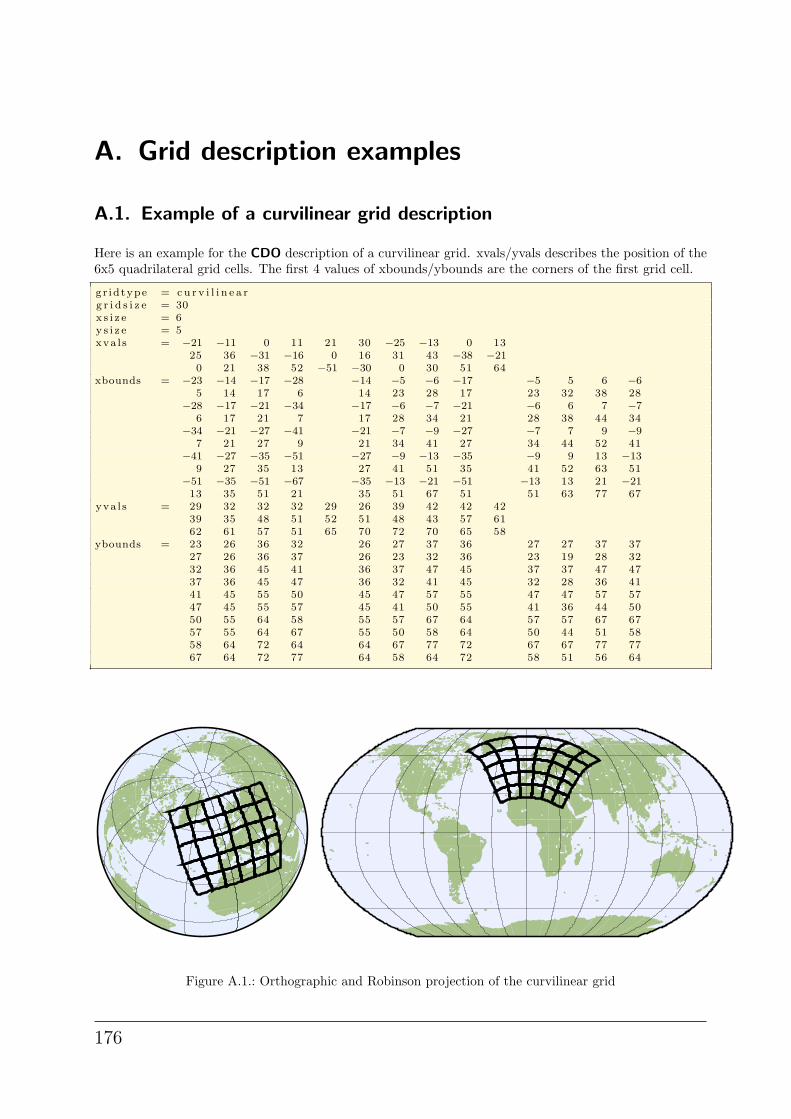
A. Grid description examples
A.1. Example of a curvilinear grid description
Here is an example for the CDO description of a curvilinear grid. xvals/yvals describes the position of the6x5 quadrilateral grid cells. The first 4 values of xbounds/ybounds are the corners of the first grid cell.
gr id type = cu r v i l i n e a rg r i d s i z e = 30x s i z e = 6y s i z e = 5xva l s = −21 −11 0 11 21 30 −25 −13 0 13
25 36 −31 −16 0 16 31 43 −38 −210 21 38 52 −51 −30 0 30 51 64
xbounds = −23 −14 −17 −28 −14 −5 −6 −17 −5 5 6 −65 14 17 6 14 23 28 17 23 32 38 28
−28 −17 −21 −34 −17 −6 −7 −21 −6 6 7 −76 17 21 7 17 28 34 21 28 38 44 34
−34 −21 −27 −41 −21 −7 −9 −27 −7 7 9 −97 21 27 9 21 34 41 27 34 44 52 41
−41 −27 −35 −51 −27 −9 −13 −35 −9 9 13 −139 27 35 13 27 41 51 35 41 52 63 51
−51 −35 −51 −67 −35 −13 −21 −51 −13 13 21 −2113 35 51 21 35 51 67 51 51 63 77 67
yva l s = 29 32 32 32 29 26 39 42 42 4239 35 48 51 52 51 48 43 57 6162 61 57 51 65 70 72 70 65 58
ybounds = 23 26 36 32 26 27 37 36 27 27 37 3727 26 36 37 26 23 32 36 23 19 28 3232 36 45 41 36 37 47 45 37 37 47 4737 36 45 47 36 32 41 45 32 28 36 4141 45 55 50 45 47 57 55 47 47 57 5747 45 55 57 45 41 50 55 41 36 44 5050 55 64 58 55 57 67 64 57 57 67 6757 55 64 67 55 50 58 64 50 44 51 5858 64 72 64 64 67 77 72 67 67 77 7767 64 72 77 64 58 64 72 58 51 56 64
Figure A.1.: Orthographic and Robinson projection of the curvilinear grid
176
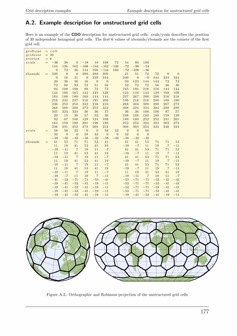
Grid description examples Example description for unstructured grid cells
A.2. Example description for unstructured grid cells
Here is an example of the CDO description for unstructured grid cells. xvals/yvals describes the positionof 30 independent hexagonal grid cells. The first 6 values of xbounds/ybounds are the corners of the firstgrid cell.
gr id type = c e l lg r i d s i z e = 30nvertex = 6xva l s = −36 36 0 −18 18 108 72 54 90 180
144 126 162 −108 −144 −162 −126 −72 −90 −540 72 36 144 108 −144 180 −72 −108 −36
xbounds = 339 0 0 288 288 309 21 51 72 72 0 00 16 21 0 339 344 340 0 −0 344 324 324
20 36 36 16 0 0 93 123 144 144 72 7272 88 93 72 51 56 52 72 72 56 36 3692 108 108 88 72 72 165 195 216 216 144 144
144 160 165 144 123 128 124 144 144 128 108 108164 180 180 160 144 144 237 267 288 288 216 216216 232 237 216 195 200 196 216 216 200 180 180236 252 252 232 216 216 288 304 309 288 267 272268 288 288 272 252 252 308 324 324 304 288 288345 324 324 36 36 15 36 36 108 108 87 5720 15 36 57 52 36 108 108 180 180 159 12992 87 108 129 124 108 180 180 252 252 231 201
164 159 180 201 196 180 252 252 324 324 303 273236 231 252 273 268 252 308 303 324 345 340 324
yva l s = 58 58 32 0 0 58 32 0 0 5832 0 0 58 32 0 0 32 0 0
−58 −58 −32 −58 −32 −58 −32 −58 −32 −32ybounds = 41 53 71 71 53 41 41 41 53 71 71 53
11 19 41 53 41 19 −19 −7 11 19 7 −11−19 −11 7 19 11 −7 41 41 53 71 71 5311 19 41 53 41 19 −19 −7 11 19 7 −11
−19 −11 7 19 11 −7 41 41 53 71 71 5311 19 41 53 41 19 −19 −7 11 19 7 −11
−19 −11 7 19 11 −7 41 41 53 71 71 5311 19 41 53 41 19 −19 −7 11 19 7 −11
−19 −11 7 19 11 −7 11 19 41 53 41 19−19 −7 11 19 7 −11 −19 −11 7 19 11 −7−41 −53 −71 −71 −53 −41 −53 −71 −71 −53 −41 −41−19 −41 −53 −41 −19 −11 −53 −71 −71 −53 −41 −41−19 −41 −53 −41 −19 −11 −53 −71 −71 −53 −41 −41−19 −41 −53 −41 −19 −11 −53 −71 −71 −53 −41 −41−19 −41 −53 −41 −19 −11 −19 −41 −53 −41 −19 −11
Figure A.2.: Orthographic and Robinson projection of the unstructured grid cells
177
Operator index
Aabs . . . . . . . . . . . . . . . . . . . . . . . . . . . . . . . . . . . . . . . . 61acos . . . . . . . . . . . . . . . . . . . . . . . . . . . . . . . . . . . . . . . 61add . . . . . . . . . . . . . . . . . . . . . . . . . . . . . . . . . . . . . . . . 63addc . . . . . . . . . . . . . . . . . . . . . . . . . . . . . . . . . . . . . . . 62asin . . . . . . . . . . . . . . . . . . . . . . . . . . . . . . . . . . . . . . . . 61atan2 . . . . . . . . . . . . . . . . . . . . . . . . . . . . . . . . . . . . . . 63
Bbandpass . . . . . . . . . . . . . . . . . . . . . . . . . . . . . . . . . 145
Ccat . . . . . . . . . . . . . . . . . . . . . . . . . . . . . . . . . . . . . . . . 25chcode . . . . . . . . . . . . . . . . . . . . . . . . . . . . . . . . . . . . . 48chlevel . . . . . . . . . . . . . . . . . . . . . . . . . . . . . . . . . . . . . 48chlevelc . . . . . . . . . . . . . . . . . . . . . . . . . . . . . . . . . . . . 48chlevelv . . . . . . . . . . . . . . . . . . . . . . . . . . . . . . . . . . . . 48chname . . . . . . . . . . . . . . . . . . . . . . . . . . . . . . . . . . . . 48consecsum . . . . . . . . . . . . . . . . . . . . . . . . . . . . . . . . . 73consects . . . . . . . . . . . . . . . . . . . . . . . . . . . . . . . . . . . 73const . . . . . . . . . . . . . . . . . . . . . . . . . . . . . . . . . . . . . 148copy . . . . . . . . . . . . . . . . . . . . . . . . . . . . . . . . . . . . . . . 25cos . . . . . . . . . . . . . . . . . . . . . . . . . . . . . . . . . . . . . . . . 61
Ddayavg . . . . . . . . . . . . . . . . . . . . . . . . . . . . . . . . . . . . . 94daymax . . . . . . . . . . . . . . . . . . . . . . . . . . . . . . . . . . . . 94daymean . . . . . . . . . . . . . . . . . . . . . . . . . . . . . . . . . . . 94daymin . . . . . . . . . . . . . . . . . . . . . . . . . . . . . . . . . . . . 94daypctl . . . . . . . . . . . . . . . . . . . . . . . . . . . . . . . . . . . . 95daystd . . . . . . . . . . . . . . . . . . . . . . . . . . . . . . . . . . . . . 94daysum . . . . . . . . . . . . . . . . . . . . . . . . . . . . . . . . . . . . 94dayvar . . . . . . . . . . . . . . . . . . . . . . . . . . . . . . . . . . . . . 94delcode . . . . . . . . . . . . . . . . . . . . . . . . . . . . . . . . . . . . 32delname . . . . . . . . . . . . . . . . . . . . . . . . . . . . . . . . . . . 32detrend . . . . . . . . . . . . . . . . . . . . . . . . . . . . . . . . . . . 115diff . . . . . . . . . . . . . . . . . . . . . . . . . . . . . . . . . . . . . . . . 20diffv . . . . . . . . . . . . . . . . . . . . . . . . . . . . . . . . . . . . . . . 20div . . . . . . . . . . . . . . . . . . . . . . . . . . . . . . . . . . . . . . . . 63divc . . . . . . . . . . . . . . . . . . . . . . . . . . . . . . . . . . . . . . . 62divdpm . . . . . . . . . . . . . . . . . . . . . . . . . . . . . . . . . . . . 67divdpy . . . . . . . . . . . . . . . . . . . . . . . . . . . . . . . . . . . . . 67dv2ps . . . . . . . . . . . . . . . . . . . . . . . . . . . . . . . . . . . . . 136dv2uv . . . . . . . . . . . . . . . . . . . . . . . . . . . . . . . . . . . . 136dv2uvl . . . . . . . . . . . . . . . . . . . . . . . . . . . . . . . . . . . . 136
Eeca cdd . . . . . . . . . . . . . . . . . . . . . . . . . . . . . . . . . . . 155eca cfd . . . . . . . . . . . . . . . . . . . . . . . . . . . . . . . . . . . 155eca csu . . . . . . . . . . . . . . . . . . . . . . . . . . . . . . . . . . . 156
eca cwd . . . . . . . . . . . . . . . . . . . . . . . . . . . . . . . . . . 156eca cwdi . . . . . . . . . . . . . . . . . . . . . . . . . . . . . . . . . . 157eca cwfi . . . . . . . . . . . . . . . . . . . . . . . . . . . . . . . . . . 157eca etr . . . . . . . . . . . . . . . . . . . . . . . . . . . . . . . . . . . . 159eca fd . . . . . . . . . . . . . . . . . . . . . . . . . . . . . . . . . . . . 159eca gsl . . . . . . . . . . . . . . . . . . . . . . . . . . . . . . . . . . . . 160eca hd . . . . . . . . . . . . . . . . . . . . . . . . . . . . . . . . . . . . 161eca hwdi . . . . . . . . . . . . . . . . . . . . . . . . . . . . . . . . . . 161eca hwfi . . . . . . . . . . . . . . . . . . . . . . . . . . . . . . . . . . 162eca id . . . . . . . . . . . . . . . . . . . . . . . . . . . . . . . . . . . . . 162eca pd . . . . . . . . . . . . . . . . . . . . . . . . . . . . . . . . . . . . 163eca r10mm . . . . . . . . . . . . . . . . . . . . . . . . . . . . . . . 163eca r20mm . . . . . . . . . . . . . . . . . . . . . . . . . . . . . . . 163eca r75p . . . . . . . . . . . . . . . . . . . . . . . . . . . . . . . . . . 164eca r75ptot . . . . . . . . . . . . . . . . . . . . . . . . . . . . . . . 164eca r90p . . . . . . . . . . . . . . . . . . . . . . . . . . . . . . . . . . 165eca r90ptot . . . . . . . . . . . . . . . . . . . . . . . . . . . . . . . 165eca r95p . . . . . . . . . . . . . . . . . . . . . . . . . . . . . . . . . . 166eca r95ptot . . . . . . . . . . . . . . . . . . . . . . . . . . . . . . . 166eca r99p . . . . . . . . . . . . . . . . . . . . . . . . . . . . . . . . . . 167eca r99ptot . . . . . . . . . . . . . . . . . . . . . . . . . . . . . . . 167eca rr1 . . . . . . . . . . . . . . . . . . . . . . . . . . . . . . . . . . . 168eca rx1day . . . . . . . . . . . . . . . . . . . . . . . . . . . . . . . . 168eca rx5day . . . . . . . . . . . . . . . . . . . . . . . . . . . . . . . . 169eca sdii . . . . . . . . . . . . . . . . . . . . . . . . . . . . . . . . . . . 169eca su . . . . . . . . . . . . . . . . . . . . . . . . . . . . . . . . . . . . 170eca tg10p . . . . . . . . . . . . . . . . . . . . . . . . . . . . . . . . . 171eca tg90p . . . . . . . . . . . . . . . . . . . . . . . . . . . . . . . . . 171eca tn10p . . . . . . . . . . . . . . . . . . . . . . . . . . . . . . . . . 172eca tn90p . . . . . . . . . . . . . . . . . . . . . . . . . . . . . . . . . 172eca tr . . . . . . . . . . . . . . . . . . . . . . . . . . . . . . . . . . . . . 173eca tx10p . . . . . . . . . . . . . . . . . . . . . . . . . . . . . . . . . 173eca tx90p . . . . . . . . . . . . . . . . . . . . . . . . . . . . . . . . . 174enlarge . . . . . . . . . . . . . . . . . . . . . . . . . . . . . . . . . . . . 55ensavg . . . . . . . . . . . . . . . . . . . . . . . . . . . . . . . . . . . . . 74ensbrs . . . . . . . . . . . . . . . . . . . . . . . . . . . . . . . . . . . . . 76enscrps . . . . . . . . . . . . . . . . . . . . . . . . . . . . . . . . . . . . 76ensmax . . . . . . . . . . . . . . . . . . . . . . . . . . . . . . . . . . . . 74ensmean . . . . . . . . . . . . . . . . . . . . . . . . . . . . . . . . . . . 74ensmin . . . . . . . . . . . . . . . . . . . . . . . . . . . . . . . . . . . . . 74enspctl . . . . . . . . . . . . . . . . . . . . . . . . . . . . . . . . . . . . 74ensrkhistspace . . . . . . . . . . . . . . . . . . . . . . . . . . . . . 76ensrkhisttime . . . . . . . . . . . . . . . . . . . . . . . . . . . . . . 76ensroc . . . . . . . . . . . . . . . . . . . . . . . . . . . . . . . . . . . . . 76ensstd . . . . . . . . . . . . . . . . . . . . . . . . . . . . . . . . . . . . . 74enssum . . . . . . . . . . . . . . . . . . . . . . . . . . . . . . . . . . . . 74ensvar . . . . . . . . . . . . . . . . . . . . . . . . . . . . . . . . . . . . . 74eof . . . . . . . . . . . . . . . . . . . . . . . . . . . . . . . . . . . . . . . . 118eof3d . . . . . . . . . . . . . . . . . . . . . . . . . . . . . . . . . . . . . 118
178
Operator index Operator index
eofcoeff . . . . . . . . . . . . . . . . . . . . . . . . . . . . . . . . . . . 120eofspatial . . . . . . . . . . . . . . . . . . . . . . . . . . . . . . . . . 118eoftime . . . . . . . . . . . . . . . . . . . . . . . . . . . . . . . . . . . 118eq . . . . . . . . . . . . . . . . . . . . . . . . . . . . . . . . . . . . . . . . . 42eqc . . . . . . . . . . . . . . . . . . . . . . . . . . . . . . . . . . . . . . . . 43exp . . . . . . . . . . . . . . . . . . . . . . . . . . . . . . . . . . . . . . . . 61expr . . . . . . . . . . . . . . . . . . . . . . . . . . . . . . . . . . . . . . . 59exprf . . . . . . . . . . . . . . . . . . . . . . . . . . . . . . . . . . . . . . 59
Ffdns . . . . . . . . . . . . . . . . . . . . . . . . . . . . . . . . . . . . . . 151fldavg . . . . . . . . . . . . . . . . . . . . . . . . . . . . . . . . . . . . . . 78fldcor . . . . . . . . . . . . . . . . . . . . . . . . . . . . . . . . . . . . . 113fldmax . . . . . . . . . . . . . . . . . . . . . . . . . . . . . . . . . . . . . 78fldmean . . . . . . . . . . . . . . . . . . . . . . . . . . . . . . . . . . . . 78fldmin . . . . . . . . . . . . . . . . . . . . . . . . . . . . . . . . . . . . . 78fldpctl . . . . . . . . . . . . . . . . . . . . . . . . . . . . . . . . . . . . . 78fldstd . . . . . . . . . . . . . . . . . . . . . . . . . . . . . . . . . . . . . . 78fldsum . . . . . . . . . . . . . . . . . . . . . . . . . . . . . . . . . . . . . 78fldvar . . . . . . . . . . . . . . . . . . . . . . . . . . . . . . . . . . . . . . 78
Gge . . . . . . . . . . . . . . . . . . . . . . . . . . . . . . . . . . . . . . . . . 42gec . . . . . . . . . . . . . . . . . . . . . . . . . . . . . . . . . . . . . . . . 43genbic . . . . . . . . . . . . . . . . . . . . . . . . . . . . . . . . . . . . 124genbil . . . . . . . . . . . . . . . . . . . . . . . . . . . . . . . . . . . . . 124gencon . . . . . . . . . . . . . . . . . . . . . . . . . . . . . . . . . . . . 124gencon2 . . . . . . . . . . . . . . . . . . . . . . . . . . . . . . . . . . 124gendis . . . . . . . . . . . . . . . . . . . . . . . . . . . . . . . . . . . . 124genlaf . . . . . . . . . . . . . . . . . . . . . . . . . . . . . . . . . . . . . 124gennn . . . . . . . . . . . . . . . . . . . . . . . . . . . . . . . . . . . . 124gp2sp . . . . . . . . . . . . . . . . . . . . . . . . . . . . . . . . . . . . . 134gp2spl . . . . . . . . . . . . . . . . . . . . . . . . . . . . . . . . . . . . 134gradsdes1 . . . . . . . . . . . . . . . . . . . . . . . . . . . . . . . . . 144gradsdes2 . . . . . . . . . . . . . . . . . . . . . . . . . . . . . . . . . 144gridarea . . . . . . . . . . . . . . . . . . . . . . . . . . . . . . . . . . 146gridboxavg . . . . . . . . . . . . . . . . . . . . . . . . . . . . . . . . . 84gridboxmax . . . . . . . . . . . . . . . . . . . . . . . . . . . . . . . . 84gridboxmean . . . . . . . . . . . . . . . . . . . . . . . . . . . . . . . 84gridboxmin . . . . . . . . . . . . . . . . . . . . . . . . . . . . . . . . 84gridboxstd . . . . . . . . . . . . . . . . . . . . . . . . . . . . . . . . . 84gridboxsum . . . . . . . . . . . . . . . . . . . . . . . . . . . . . . . . 84gridboxvar . . . . . . . . . . . . . . . . . . . . . . . . . . . . . . . . . 84griddes . . . . . . . . . . . . . . . . . . . . . . . . . . . . . . . . . . . . 23gridweights . . . . . . . . . . . . . . . . . . . . . . . . . . . . . . . 146gt . . . . . . . . . . . . . . . . . . . . . . . . . . . . . . . . . . . . . . . . . 42gtc . . . . . . . . . . . . . . . . . . . . . . . . . . . . . . . . . . . . . . . . 43
Hhighpass . . . . . . . . . . . . . . . . . . . . . . . . . . . . . . . . . . 145histcount . . . . . . . . . . . . . . . . . . . . . . . . . . . . . . . . . 150histfreq . . . . . . . . . . . . . . . . . . . . . . . . . . . . . . . . . . . 150histmean . . . . . . . . . . . . . . . . . . . . . . . . . . . . . . . . . 150histsum . . . . . . . . . . . . . . . . . . . . . . . . . . . . . . . . . . . 150houravg . . . . . . . . . . . . . . . . . . . . . . . . . . . . . . . . . . . . 92hourmax . . . . . . . . . . . . . . . . . . . . . . . . . . . . . . . . . . . 92hourmean . . . . . . . . . . . . . . . . . . . . . . . . . . . . . . . . . . 92hourmin . . . . . . . . . . . . . . . . . . . . . . . . . . . . . . . . . . . 92
hourpctl . . . . . . . . . . . . . . . . . . . . . . . . . . . . . . . . . . . 93hourstd . . . . . . . . . . . . . . . . . . . . . . . . . . . . . . . . . . . . 92hoursum . . . . . . . . . . . . . . . . . . . . . . . . . . . . . . . . . . . 92hourvar . . . . . . . . . . . . . . . . . . . . . . . . . . . . . . . . . . . . 92hurr . . . . . . . . . . . . . . . . . . . . . . . . . . . . . . . . . . . . . . 152
Iifnotthen . . . . . . . . . . . . . . . . . . . . . . . . . . . . . . . . . . 38ifnotthenc . . . . . . . . . . . . . . . . . . . . . . . . . . . . . . . . . 40ifthen . . . . . . . . . . . . . . . . . . . . . . . . . . . . . . . . . . . . . . 38ifthenc . . . . . . . . . . . . . . . . . . . . . . . . . . . . . . . . . . . . . 40ifthenelse . . . . . . . . . . . . . . . . . . . . . . . . . . . . . . . . . . 38import amsr . . . . . . . . . . . . . . . . . . . . . . . . . . . . . . 140import binary . . . . . . . . . . . . . . . . . . . . . . . . . . . . 138import cmsaf . . . . . . . . . . . . . . . . . . . . . . . . . . . . . 139info . . . . . . . . . . . . . . . . . . . . . . . . . . . . . . . . . . . . . . . . 18infov . . . . . . . . . . . . . . . . . . . . . . . . . . . . . . . . . . . . . . . 18input . . . . . . . . . . . . . . . . . . . . . . . . . . . . . . . . . . . . . 141inputext . . . . . . . . . . . . . . . . . . . . . . . . . . . . . . . . . . 141inputsrv . . . . . . . . . . . . . . . . . . . . . . . . . . . . . . . . . . 141int . . . . . . . . . . . . . . . . . . . . . . . . . . . . . . . . . . . . . . . . . 61intlevel . . . . . . . . . . . . . . . . . . . . . . . . . . . . . . . . . . . 130intntime . . . . . . . . . . . . . . . . . . . . . . . . . . . . . . . . . . 131inttime . . . . . . . . . . . . . . . . . . . . . . . . . . . . . . . . . . . 131intyear . . . . . . . . . . . . . . . . . . . . . . . . . . . . . . . . . . . . 132invertlat . . . . . . . . . . . . . . . . . . . . . . . . . . . . . . . . . . . 51invertlev . . . . . . . . . . . . . . . . . . . . . . . . . . . . . . . . . . . 51
Lle . . . . . . . . . . . . . . . . . . . . . . . . . . . . . . . . . . . . . . . . . . 42lec . . . . . . . . . . . . . . . . . . . . . . . . . . . . . . . . . . . . . . . . . 43ln . . . . . . . . . . . . . . . . . . . . . . . . . . . . . . . . . . . . . . . . . . 61log10 . . . . . . . . . . . . . . . . . . . . . . . . . . . . . . . . . . . . . . 61lowpass . . . . . . . . . . . . . . . . . . . . . . . . . . . . . . . . . . . 145lt . . . . . . . . . . . . . . . . . . . . . . . . . . . . . . . . . . . . . . . . . . 42ltc . . . . . . . . . . . . . . . . . . . . . . . . . . . . . . . . . . . . . . . . . 43
Mmap . . . . . . . . . . . . . . . . . . . . . . . . . . . . . . . . . . . . . . . 18maskindexbox . . . . . . . . . . . . . . . . . . . . . . . . . . . . . 53masklonlatbox . . . . . . . . . . . . . . . . . . . . . . . . . . . . . 53maskregion . . . . . . . . . . . . . . . . . . . . . . . . . . . . . . . . 52mastrfu . . . . . . . . . . . . . . . . . . . . . . . . . . . . . . . . . . . 149max . . . . . . . . . . . . . . . . . . . . . . . . . . . . . . . . . . . . . . . 63meravg . . . . . . . . . . . . . . . . . . . . . . . . . . . . . . . . . . . . 82merge . . . . . . . . . . . . . . . . . . . . . . . . . . . . . . . . . . . . . . 27mergetime . . . . . . . . . . . . . . . . . . . . . . . . . . . . . . . . . 27mermax . . . . . . . . . . . . . . . . . . . . . . . . . . . . . . . . . . . 82mermean . . . . . . . . . . . . . . . . . . . . . . . . . . . . . . . . . . 82mermin . . . . . . . . . . . . . . . . . . . . . . . . . . . . . . . . . . . . 82merpctl . . . . . . . . . . . . . . . . . . . . . . . . . . . . . . . . . . . . 82merstd . . . . . . . . . . . . . . . . . . . . . . . . . . . . . . . . . . . . . 82mersum . . . . . . . . . . . . . . . . . . . . . . . . . . . . . . . . . . . . 82mervar . . . . . . . . . . . . . . . . . . . . . . . . . . . . . . . . . . . . . 82min . . . . . . . . . . . . . . . . . . . . . . . . . . . . . . . . . . . . . . . . 63ml2hl . . . . . . . . . . . . . . . . . . . . . . . . . . . . . . . . . . . . . 129ml2pl . . . . . . . . . . . . . . . . . . . . . . . . . . . . . . . . . . . . . 129monadd . . . . . . . . . . . . . . . . . . . . . . . . . . . . . . . . . . . . 64
179
Operator index Operator index
monavg . . . . . . . . . . . . . . . . . . . . . . . . . . . . . . . . . . . . 96mondiv . . . . . . . . . . . . . . . . . . . . . . . . . . . . . . . . . . . . 64monmax . . . . . . . . . . . . . . . . . . . . . . . . . . . . . . . . . . . 96monmean . . . . . . . . . . . . . . . . . . . . . . . . . . . . . . . . . . 96monmin . . . . . . . . . . . . . . . . . . . . . . . . . . . . . . . . . . . 96monmul . . . . . . . . . . . . . . . . . . . . . . . . . . . . . . . . . . . . 64monpctl . . . . . . . . . . . . . . . . . . . . . . . . . . . . . . . . . . . 97monstd . . . . . . . . . . . . . . . . . . . . . . . . . . . . . . . . . . . . 96monsub . . . . . . . . . . . . . . . . . . . . . . . . . . . . . . . . . . . . 64monsum . . . . . . . . . . . . . . . . . . . . . . . . . . . . . . . . . . . 96monvar . . . . . . . . . . . . . . . . . . . . . . . . . . . . . . . . . . . . 96mul . . . . . . . . . . . . . . . . . . . . . . . . . . . . . . . . . . . . . . . . 63mulc . . . . . . . . . . . . . . . . . . . . . . . . . . . . . . . . . . . . . . . 62muldpm . . . . . . . . . . . . . . . . . . . . . . . . . . . . . . . . . . . 67muldpy . . . . . . . . . . . . . . . . . . . . . . . . . . . . . . . . . . . . 67
Nndate . . . . . . . . . . . . . . . . . . . . . . . . . . . . . . . . . . . . . . 21ne . . . . . . . . . . . . . . . . . . . . . . . . . . . . . . . . . . . . . . . . . 42nec . . . . . . . . . . . . . . . . . . . . . . . . . . . . . . . . . . . . . . . . 43nint . . . . . . . . . . . . . . . . . . . . . . . . . . . . . . . . . . . . . . . . 61nlevel . . . . . . . . . . . . . . . . . . . . . . . . . . . . . . . . . . . . . . 21nmon . . . . . . . . . . . . . . . . . . . . . . . . . . . . . . . . . . . . . . 21npar . . . . . . . . . . . . . . . . . . . . . . . . . . . . . . . . . . . . . . . 21ntime . . . . . . . . . . . . . . . . . . . . . . . . . . . . . . . . . . . . . . 21nyear . . . . . . . . . . . . . . . . . . . . . . . . . . . . . . . . . . . . . . 21
Ooutput . . . . . . . . . . . . . . . . . . . . . . . . . . . . . . . . . . . . 142outputext . . . . . . . . . . . . . . . . . . . . . . . . . . . . . . . . . 142outputf . . . . . . . . . . . . . . . . . . . . . . . . . . . . . . . . . . . 142outputint . . . . . . . . . . . . . . . . . . . . . . . . . . . . . . . . . 142outputsrv . . . . . . . . . . . . . . . . . . . . . . . . . . . . . . . . . 142
Ppardes . . . . . . . . . . . . . . . . . . . . . . . . . . . . . . . . . . . . . 23pow . . . . . . . . . . . . . . . . . . . . . . . . . . . . . . . . . . . . . . . 61
Rrandom . . . . . . . . . . . . . . . . . . . . . . . . . . . . . . . . . . . 148reci . . . . . . . . . . . . . . . . . . . . . . . . . . . . . . . . . . . . . . . . 61regres . . . . . . . . . . . . . . . . . . . . . . . . . . . . . . . . . . . . . 115remap . . . . . . . . . . . . . . . . . . . . . . . . . . . . . . . . . . . . 126remapbic . . . . . . . . . . . . . . . . . . . . . . . . . . . . . . . . . 122remapbil . . . . . . . . . . . . . . . . . . . . . . . . . . . . . . . . . . 122remapcon . . . . . . . . . . . . . . . . . . . . . . . . . . . . . . . . . 122remapcon2 . . . . . . . . . . . . . . . . . . . . . . . . . . . . . . . . 122remapdis . . . . . . . . . . . . . . . . . . . . . . . . . . . . . . . . . 122remapeta . . . . . . . . . . . . . . . . . . . . . . . . . . . . . . . . . 127remaplaf . . . . . . . . . . . . . . . . . . . . . . . . . . . . . . . . . . 122remapnn . . . . . . . . . . . . . . . . . . . . . . . . . . . . . . . . . . 122replace . . . . . . . . . . . . . . . . . . . . . . . . . . . . . . . . . . . . . 25rotuvb . . . . . . . . . . . . . . . . . . . . . . . . . . . . . . . . . . . . 149runavg . . . . . . . . . . . . . . . . . . . . . . . . . . . . . . . . . . . . . 88runmax . . . . . . . . . . . . . . . . . . . . . . . . . . . . . . . . . . . . 88runmean . . . . . . . . . . . . . . . . . . . . . . . . . . . . . . . . . . . 88runmin . . . . . . . . . . . . . . . . . . . . . . . . . . . . . . . . . . . . 88runpctl . . . . . . . . . . . . . . . . . . . . . . . . . . . . . . . . . . . . 89
runstd . . . . . . . . . . . . . . . . . . . . . . . . . . . . . . . . . . . . . 88runsum . . . . . . . . . . . . . . . . . . . . . . . . . . . . . . . . . . . . 88runvar . . . . . . . . . . . . . . . . . . . . . . . . . . . . . . . . . . . . . 88
Sseasavg . . . . . . . . . . . . . . . . . . . . . . . . . . . . . . . . . . . 100seasmax . . . . . . . . . . . . . . . . . . . . . . . . . . . . . . . . . . 100seasmean . . . . . . . . . . . . . . . . . . . . . . . . . . . . . . . . . 100seasmin . . . . . . . . . . . . . . . . . . . . . . . . . . . . . . . . . . . 100seaspctl . . . . . . . . . . . . . . . . . . . . . . . . . . . . . . . . . . . 101seasstd . . . . . . . . . . . . . . . . . . . . . . . . . . . . . . . . . . . 100seassum . . . . . . . . . . . . . . . . . . . . . . . . . . . . . . . . . . 100seasvar . . . . . . . . . . . . . . . . . . . . . . . . . . . . . . . . . . . 100selcode . . . . . . . . . . . . . . . . . . . . . . . . . . . . . . . . . . . . 32seldate . . . . . . . . . . . . . . . . . . . . . . . . . . . . . . . . . . . . . 34selday . . . . . . . . . . . . . . . . . . . . . . . . . . . . . . . . . . . . . 34selgrid . . . . . . . . . . . . . . . . . . . . . . . . . . . . . . . . . . . . . 32selhour . . . . . . . . . . . . . . . . . . . . . . . . . . . . . . . . . . . . 34selindexbox . . . . . . . . . . . . . . . . . . . . . . . . . . . . . . . . 36sellevel . . . . . . . . . . . . . . . . . . . . . . . . . . . . . . . . . . . . . 32sellevidx . . . . . . . . . . . . . . . . . . . . . . . . . . . . . . . . . . . 32sellonlatbox . . . . . . . . . . . . . . . . . . . . . . . . . . . . . . . . 36selltype . . . . . . . . . . . . . . . . . . . . . . . . . . . . . . . . . . . . 32selmon . . . . . . . . . . . . . . . . . . . . . . . . . . . . . . . . . . . . . 34selname . . . . . . . . . . . . . . . . . . . . . . . . . . . . . . . . . . . . 32selseas . . . . . . . . . . . . . . . . . . . . . . . . . . . . . . . . . . . . . 34selsmon . . . . . . . . . . . . . . . . . . . . . . . . . . . . . . . . . . . . 34selstdname . . . . . . . . . . . . . . . . . . . . . . . . . . . . . . . . . 32seltabnum . . . . . . . . . . . . . . . . . . . . . . . . . . . . . . . . . 32seltime . . . . . . . . . . . . . . . . . . . . . . . . . . . . . . . . . . . . . 34seltimestep . . . . . . . . . . . . . . . . . . . . . . . . . . . . . . . . . 34selyear . . . . . . . . . . . . . . . . . . . . . . . . . . . . . . . . . . . . . 34selzaxis . . . . . . . . . . . . . . . . . . . . . . . . . . . . . . . . . . . . 32setcalendar . . . . . . . . . . . . . . . . . . . . . . . . . . . . . . . . 46setcindexbox . . . . . . . . . . . . . . . . . . . . . . . . . . . . . . . 54setclonlatbox . . . . . . . . . . . . . . . . . . . . . . . . . . . . . . 54setcode . . . . . . . . . . . . . . . . . . . . . . . . . . . . . . . . . . . . 45setctomiss . . . . . . . . . . . . . . . . . . . . . . . . . . . . . . . . . 56setdate . . . . . . . . . . . . . . . . . . . . . . . . . . . . . . . . . . . . 46setday . . . . . . . . . . . . . . . . . . . . . . . . . . . . . . . . . . . . . 46setgatt . . . . . . . . . . . . . . . . . . . . . . . . . . . . . . . . . . . . . 50setgatts . . . . . . . . . . . . . . . . . . . . . . . . . . . . . . . . . . . . 50setgrid . . . . . . . . . . . . . . . . . . . . . . . . . . . . . . . . . . . . . 49setgridtype . . . . . . . . . . . . . . . . . . . . . . . . . . . . . . . . 49sethalo . . . . . . . . . . . . . . . . . . . . . . . . . . . . . . . . . . . 150setlevel . . . . . . . . . . . . . . . . . . . . . . . . . . . . . . . . . . . . 45setltype . . . . . . . . . . . . . . . . . . . . . . . . . . . . . . . . . . . . 45setmisstoc . . . . . . . . . . . . . . . . . . . . . . . . . . . . . . . . . 56setmissval . . . . . . . . . . . . . . . . . . . . . . . . . . . . . . . . . . 56setmon . . . . . . . . . . . . . . . . . . . . . . . . . . . . . . . . . . . . 46setname . . . . . . . . . . . . . . . . . . . . . . . . . . . . . . . . . . . 45setpartab . . . . . . . . . . . . . . . . . . . . . . . . . . . . . . . . . . 45setreftime . . . . . . . . . . . . . . . . . . . . . . . . . . . . . . . . . . 46setrtoc . . . . . . . . . . . . . . . . . . . . . . . . . . . . . . . . . . . . 147setrtoc2 . . . . . . . . . . . . . . . . . . . . . . . . . . . . . . . . . . 147setrtomiss . . . . . . . . . . . . . . . . . . . . . . . . . . . . . . . . . 56settaxis . . . . . . . . . . . . . . . . . . . . . . . . . . . . . . . . . . . . 46settime . . . . . . . . . . . . . . . . . . . . . . . . . . . . . . . . . . . . 46
180
Operator index Operator index
settunits . . . . . . . . . . . . . . . . . . . . . . . . . . . . . . . . . . . 46setvals . . . . . . . . . . . . . . . . . . . . . . . . . . . . . . . . . . . . 147setvrange . . . . . . . . . . . . . . . . . . . . . . . . . . . . . . . . . . 56setyear . . . . . . . . . . . . . . . . . . . . . . . . . . . . . . . . . . . . . 46setzaxis . . . . . . . . . . . . . . . . . . . . . . . . . . . . . . . . . . . . 49shifttime . . . . . . . . . . . . . . . . . . . . . . . . . . . . . . . . . . . 46showcode . . . . . . . . . . . . . . . . . . . . . . . . . . . . . . . . . . 22showdate . . . . . . . . . . . . . . . . . . . . . . . . . . . . . . . . . . 22showformat . . . . . . . . . . . . . . . . . . . . . . . . . . . . . . . . 22showlevel . . . . . . . . . . . . . . . . . . . . . . . . . . . . . . . . . . 22showltype . . . . . . . . . . . . . . . . . . . . . . . . . . . . . . . . . . 22showmon . . . . . . . . . . . . . . . . . . . . . . . . . . . . . . . . . . 22showname . . . . . . . . . . . . . . . . . . . . . . . . . . . . . . . . . 22showstdname . . . . . . . . . . . . . . . . . . . . . . . . . . . . . . 22showtime . . . . . . . . . . . . . . . . . . . . . . . . . . . . . . . . . . 22showtimestamp . . . . . . . . . . . . . . . . . . . . . . . . . . . . 22showyear . . . . . . . . . . . . . . . . . . . . . . . . . . . . . . . . . . 22sin . . . . . . . . . . . . . . . . . . . . . . . . . . . . . . . . . . . . . . . . . 61sinfo . . . . . . . . . . . . . . . . . . . . . . . . . . . . . . . . . . . . . . . 19sinfop . . . . . . . . . . . . . . . . . . . . . . . . . . . . . . . . . . . . . . 19sinfov . . . . . . . . . . . . . . . . . . . . . . . . . . . . . . . . . . . . . . 19smooth9 . . . . . . . . . . . . . . . . . . . . . . . . . . . . . . . . . . 147sp2gp . . . . . . . . . . . . . . . . . . . . . . . . . . . . . . . . . . . . . 134sp2gpl . . . . . . . . . . . . . . . . . . . . . . . . . . . . . . . . . . . . 134sp2sp . . . . . . . . . . . . . . . . . . . . . . . . . . . . . . . . . . . . . 134splitcode . . . . . . . . . . . . . . . . . . . . . . . . . . . . . . . . . . . 28splitday . . . . . . . . . . . . . . . . . . . . . . . . . . . . . . . . . . . . 29splitgrid . . . . . . . . . . . . . . . . . . . . . . . . . . . . . . . . . . . 28splithour . . . . . . . . . . . . . . . . . . . . . . . . . . . . . . . . . . . 29splitlevel . . . . . . . . . . . . . . . . . . . . . . . . . . . . . . . . . . . 28splitmon . . . . . . . . . . . . . . . . . . . . . . . . . . . . . . . . . . . 29splitname . . . . . . . . . . . . . . . . . . . . . . . . . . . . . . . . . . 28splitseas . . . . . . . . . . . . . . . . . . . . . . . . . . . . . . . . . . . 29splitsel . . . . . . . . . . . . . . . . . . . . . . . . . . . . . . . . . . . . . 30splittabnum . . . . . . . . . . . . . . . . . . . . . . . . . . . . . . . . 28splityear . . . . . . . . . . . . . . . . . . . . . . . . . . . . . . . . . . . 29splitzaxis . . . . . . . . . . . . . . . . . . . . . . . . . . . . . . . . . . 28sqr . . . . . . . . . . . . . . . . . . . . . . . . . . . . . . . . . . . . . . . . . 61sqrt . . . . . . . . . . . . . . . . . . . . . . . . . . . . . . . . . . . . . . . . 61strbre . . . . . . . . . . . . . . . . . . . . . . . . . . . . . . . . . . . . . 152strgal . . . . . . . . . . . . . . . . . . . . . . . . . . . . . . . . . . . . . 152strwin . . . . . . . . . . . . . . . . . . . . . . . . . . . . . . . . . . . . 151sub . . . . . . . . . . . . . . . . . . . . . . . . . . . . . . . . . . . . . . . . 63subc . . . . . . . . . . . . . . . . . . . . . . . . . . . . . . . . . . . . . . . 62subtrend . . . . . . . . . . . . . . . . . . . . . . . . . . . . . . . . . . 116
Ttan . . . . . . . . . . . . . . . . . . . . . . . . . . . . . . . . . . . . . . . . 61timavg . . . . . . . . . . . . . . . . . . . . . . . . . . . . . . . . . . . . . 90timcor . . . . . . . . . . . . . . . . . . . . . . . . . . . . . . . . . . . . 113timmax . . . . . . . . . . . . . . . . . . . . . . . . . . . . . . . . . . . . 90timmean . . . . . . . . . . . . . . . . . . . . . . . . . . . . . . . . . . . 90timmin . . . . . . . . . . . . . . . . . . . . . . . . . . . . . . . . . . . . 90timpctl . . . . . . . . . . . . . . . . . . . . . . . . . . . . . . . . . . . . 91timselavg . . . . . . . . . . . . . . . . . . . . . . . . . . . . . . . . . . 86timselmax . . . . . . . . . . . . . . . . . . . . . . . . . . . . . . . . . 86timselmean . . . . . . . . . . . . . . . . . . . . . . . . . . . . . . . . 86timselmin . . . . . . . . . . . . . . . . . . . . . . . . . . . . . . . . . . 86
timselpctl . . . . . . . . . . . . . . . . . . . . . . . . . . . . . . . . . . 87timselstd . . . . . . . . . . . . . . . . . . . . . . . . . . . . . . . . . . . 86timselsum . . . . . . . . . . . . . . . . . . . . . . . . . . . . . . . . . . 86timselvar . . . . . . . . . . . . . . . . . . . . . . . . . . . . . . . . . . 86timsort . . . . . . . . . . . . . . . . . . . . . . . . . . . . . . . . . . . 148timstd . . . . . . . . . . . . . . . . . . . . . . . . . . . . . . . . . . . . . 90timsum . . . . . . . . . . . . . . . . . . . . . . . . . . . . . . . . . . . . 90timvar . . . . . . . . . . . . . . . . . . . . . . . . . . . . . . . . . . . . . 90trend . . . . . . . . . . . . . . . . . . . . . . . . . . . . . . . . . . . . . 116
Uuv2dv . . . . . . . . . . . . . . . . . . . . . . . . . . . . . . . . . . . . 136uv2dvl . . . . . . . . . . . . . . . . . . . . . . . . . . . . . . . . . . . . 136
Vvct . . . . . . . . . . . . . . . . . . . . . . . . . . . . . . . . . . . . . . . . 23vertavg . . . . . . . . . . . . . . . . . . . . . . . . . . . . . . . . . . . . 85vertmax . . . . . . . . . . . . . . . . . . . . . . . . . . . . . . . . . . . 85vertmean . . . . . . . . . . . . . . . . . . . . . . . . . . . . . . . . . . 85vertmin . . . . . . . . . . . . . . . . . . . . . . . . . . . . . . . . . . . . 85vertstd . . . . . . . . . . . . . . . . . . . . . . . . . . . . . . . . . . . . . 85vertsum . . . . . . . . . . . . . . . . . . . . . . . . . . . . . . . . . . . . 85vertvar . . . . . . . . . . . . . . . . . . . . . . . . . . . . . . . . . . . . 85
Wwct . . . . . . . . . . . . . . . . . . . . . . . . . . . . . . . . . . . . . . . 151
Yydayadd . . . . . . . . . . . . . . . . . . . . . . . . . . . . . . . . . . . 66ydayavg . . . . . . . . . . . . . . . . . . . . . . . . . . . . . . . . . . 103ydaydiv . . . . . . . . . . . . . . . . . . . . . . . . . . . . . . . . . . . . 66ydaymax . . . . . . . . . . . . . . . . . . . . . . . . . . . . . . . . . 103ydaymean . . . . . . . . . . . . . . . . . . . . . . . . . . . . . . . . 103ydaymin . . . . . . . . . . . . . . . . . . . . . . . . . . . . . . . . . . 103ydaymul . . . . . . . . . . . . . . . . . . . . . . . . . . . . . . . . . . . 66ydaypctl . . . . . . . . . . . . . . . . . . . . . . . . . . . . . . . . . . 104ydaystd . . . . . . . . . . . . . . . . . . . . . . . . . . . . . . . . . . . 103ydaysub . . . . . . . . . . . . . . . . . . . . . . . . . . . . . . . . . . . 66ydaysum . . . . . . . . . . . . . . . . . . . . . . . . . . . . . . . . . . 103ydayvar . . . . . . . . . . . . . . . . . . . . . . . . . . . . . . . . . . . 103ydrunavg . . . . . . . . . . . . . . . . . . . . . . . . . . . . . . . . . 109ydrunmax . . . . . . . . . . . . . . . . . . . . . . . . . . . . . . . . 109ydrunmean . . . . . . . . . . . . . . . . . . . . . . . . . . . . . . . 109ydrunmin . . . . . . . . . . . . . . . . . . . . . . . . . . . . . . . . . 109ydrunpctl . . . . . . . . . . . . . . . . . . . . . . . . . . . . . . . . . 111ydrunstd . . . . . . . . . . . . . . . . . . . . . . . . . . . . . . . . . 109ydrunsum . . . . . . . . . . . . . . . . . . . . . . . . . . . . . . . . 109ydrunvar . . . . . . . . . . . . . . . . . . . . . . . . . . . . . . . . . 109yearavg . . . . . . . . . . . . . . . . . . . . . . . . . . . . . . . . . . . . 98yearmax . . . . . . . . . . . . . . . . . . . . . . . . . . . . . . . . . . . 98yearmean . . . . . . . . . . . . . . . . . . . . . . . . . . . . . . . . . . 98yearmin . . . . . . . . . . . . . . . . . . . . . . . . . . . . . . . . . . . . 98yearpctl . . . . . . . . . . . . . . . . . . . . . . . . . . . . . . . . . . . 99yearstd . . . . . . . . . . . . . . . . . . . . . . . . . . . . . . . . . . . . 98yearsum . . . . . . . . . . . . . . . . . . . . . . . . . . . . . . . . . . . 98yearvar . . . . . . . . . . . . . . . . . . . . . . . . . . . . . . . . . . . . 98yhouravg . . . . . . . . . . . . . . . . . . . . . . . . . . . . . . . . . 102yhourmax . . . . . . . . . . . . . . . . . . . . . . . . . . . . . . . . 102
181
Operator index Operator index
yhourmean . . . . . . . . . . . . . . . . . . . . . . . . . . . . . . . 102yhourmin . . . . . . . . . . . . . . . . . . . . . . . . . . . . . . . . . 102yhourstd . . . . . . . . . . . . . . . . . . . . . . . . . . . . . . . . . . 102yhoursum . . . . . . . . . . . . . . . . . . . . . . . . . . . . . . . . . 102yhourvar . . . . . . . . . . . . . . . . . . . . . . . . . . . . . . . . . . 102ymonadd . . . . . . . . . . . . . . . . . . . . . . . . . . . . . . . . . . 65ymonavg . . . . . . . . . . . . . . . . . . . . . . . . . . . . . . . . . 105ymondiv . . . . . . . . . . . . . . . . . . . . . . . . . . . . . . . . . . . 65ymonmax . . . . . . . . . . . . . . . . . . . . . . . . . . . . . . . . . 105ymonmean . . . . . . . . . . . . . . . . . . . . . . . . . . . . . . . . 105ymonmin . . . . . . . . . . . . . . . . . . . . . . . . . . . . . . . . . 105ymonmul . . . . . . . . . . . . . . . . . . . . . . . . . . . . . . . . . . 65ymonpctl . . . . . . . . . . . . . . . . . . . . . . . . . . . . . . . . . 106ymonstd . . . . . . . . . . . . . . . . . . . . . . . . . . . . . . . . . . 105ymonsub . . . . . . . . . . . . . . . . . . . . . . . . . . . . . . . . . . . 65ymonsum . . . . . . . . . . . . . . . . . . . . . . . . . . . . . . . . . 105ymonvar . . . . . . . . . . . . . . . . . . . . . . . . . . . . . . . . . . 105yseasavg . . . . . . . . . . . . . . . . . . . . . . . . . . . . . . . . . . 107yseasmax . . . . . . . . . . . . . . . . . . . . . . . . . . . . . . . . . 107yseasmean . . . . . . . . . . . . . . . . . . . . . . . . . . . . . . . . 107yseasmin . . . . . . . . . . . . . . . . . . . . . . . . . . . . . . . . . 107yseaspctl . . . . . . . . . . . . . . . . . . . . . . . . . . . . . . . . . 108yseasstd . . . . . . . . . . . . . . . . . . . . . . . . . . . . . . . . . . 107yseassum . . . . . . . . . . . . . . . . . . . . . . . . . . . . . . . . . 107yseasvar . . . . . . . . . . . . . . . . . . . . . . . . . . . . . . . . . . 107
Zzaxisdes . . . . . . . . . . . . . . . . . . . . . . . . . . . . . . . . . . . 23zonavg . . . . . . . . . . . . . . . . . . . . . . . . . . . . . . . . . . . . . 80zonmax . . . . . . . . . . . . . . . . . . . . . . . . . . . . . . . . . . . . 80zonmean . . . . . . . . . . . . . . . . . . . . . . . . . . . . . . . . . . . 80zonmin . . . . . . . . . . . . . . . . . . . . . . . . . . . . . . . . . . . . 80zonpctl . . . . . . . . . . . . . . . . . . . . . . . . . . . . . . . . . . . . 80zonstd . . . . . . . . . . . . . . . . . . . . . . . . . . . . . . . . . . . . . 80zonsum . . . . . . . . . . . . . . . . . . . . . . . . . . . . . . . . . . . . 80zonvar . . . . . . . . . . . . . . . . . . . . . . . . . . . . . . . . . . . . . 80
182


![[2021] 675 IAC 28 National Fire Protection Association (Nfpa](https://img.dokumen.tips/doc/110x75/6331d9427f0d9c38da0128bc/2021-675-iac-28-national-fire-protection-association-nfpa-.jpg)


