A Fresh Look at the Bayesian Bounds of the Weiss-Weinstein Family

5334 IEEE TRANSACTIONS ON SIGNAL PROCESSING, VOL. 56, NO. 11, NOVEMBER 2008

A Fresh Look at the Bayesian Bounds of theWeiss-Weinstein Family

Alexandre Renaux, Member, IEEE, Philippe Forster, Member, IEEE, Pascal Larzabal, Member, IEEE,Christ D. Richmond, Senior Member, IEEE, and Arye Nehorai, Fellow, IEEE

Abstract—Minimal bounds on the mean square error (MSE) aregenerally used in order to predict the best achievable performanceof an estimator for a given observation model. In this paper, we areinterested in the Bayesian bound of the Weiss–Weinstein family.Among this family, we have Bayesian Cramér-Rao bound, the Bo-brovsky–MayerWolf–Zakaï bound, the Bayesian Bhattacharyyabound, the Bobrovsky–Zakaï bound, the Reuven–Messer bound,and the Weiss–Weinstein bound. We present a unification ofall these minimal bounds based on a rewriting of the minimummean square error estimator (MMSEE) and on a constrainedoptimization problem. With this approach, we obtain a usefultheoretical framework to derive new Bayesian bounds. For thatpurpose, we propose two bounds. First, we propose a generaliza-tion of the Bayesian Bhattacharyya bound extending the worksof Bobrovsky, Mayer–Wolf, and Zakaï. Second, we propose abound based on the Bayesian Bhattacharyya bound and on theReuven–Messer bound, representing a generalization of thesebounds. The proposed bound is the Bayesian extension of thedeterministic Abel bound and is found to be tighter than theBayesian Bhattacharyya bound, the Reuven–Messer bound, theBobrovsky–Zakaï bound, and the Bayesian Cramér–Rao bound.We propose some closed-form expressions of these bounds for ageneral Gaussian observation model with parameterized mean. Inorder to illustrate our results, we present simulation results in thecontext of a spectral analysis problem.

Index Terms—Bayesian bounds on the MSE, Weiss–Weinsteinfamily.

Manuscript received April 24, 2007; revised April 18, 2008 First publishedJune 13, 2008; current version published October 15, 2008. The associate editorcoordinating the review of this manuscript and approving it for publication wasProf. Philippe Loubaton. The work of A. Renaux and A. Nehorai was supportedin part by the Department of Defense under the Air Force Office of ScientificResearch MURI Grant FA9550-05-1-0443, AFOSR Grant FA9550-05-1-0018,and by the National Science Foundation by Grants CCR-0330342 and CCF-0630734. The material in this paper was presented in part at the IEEE Workshopon Statistical Signal Processing, Bordeaux, France, July 2005 and at the IEEEInternational Conference on Acoustic, Speech and Signal Processing, Toulouse,France, May 2006.

A. Renaux is with the Laboratoire des Signaux et Systèmes, Laboratory ofSignals and Systems, University Paris-Sud 11, 91192 Gif-sur-Yvette cedex,France (e-mail: [email protected]).

P. Forster is with the Université de Nanterre, IUT de Ville d’Avray, France.He is also with the SATIE Laboratory (École Normale Supérieure de Cachan),94235 Cachan, France (e-mail: [email protected]).

P. Larzabal is with the University Paris-Sud 11, 91192 Gif-sur-Yvette cedex,France. He is also with the SATIE Laboratory (École Normale Supérieure deCachan), 94235 Cachan, France (e-mail: [email protected]).

C. D. Richmond is with the Advanced Sensor Techniques Group, LincolnLaboratory, Massachusetts Institute of Technology, Lexington, MA 02420 USA(e-mail: [email protected]).

A. Nehorai is with Washington University, St. Louis, MO 63130 USA (e-mail:[email protected]).

Color versions of one or more of the figures in this paper are available onlineat http://ieeexplore.ieee.org.

Digital Object Identifier 10.1109/TSP.2008.927075

NOTATIONS

The notational convention adopted in this paper is as follows:italic indicates a scalar quantity, as in ; lowercase boldface in-dicates a vector quantity, as in ; uppercase boldface indicates amatrix quantity, as in . is the real part of andis the imaginary part of . The complex conjugation of a quan-tity is indicated by a superscript * as in . The matrix transposeis indicated by a superscript as in , and the complex con-jugate plus matrix transpose is indicated by a superscript as in

. The -th row and -th column element of thematrix is denoted by . denotes the identity matrixof size . is a matrix of zeros. denotesthe norm. denotes the modulus. denotes the absolutevalue. denotes the Dirac delta function. denotes theexpectation operator with respect to a density probability func-tion explicitly given by a subscript. is the observation spaceand is the parameter space.

I. INTRODUCTION

M INIMAL bounds on the mean square error (MSE) pro-vide the ultimate performance that an estimator can ex-

pect to achieve for a given observation model. Consequently,they are used as a benchmark in order to evaluate the perfor-mance of an estimator and to determine if an improvement ispossible. The Cramér–Rao bound [3]–[8] has been the mostwidely used by the signal processing community and is stillunder investigation from a theoretical point of view (particu-larly throughout the differential variety in the Riemannian ge-ometry framework [9]–[14]) as from a practical point of view(see, e.g., [15]–[19]). But the Cramér–Rao bound suffers fromsome drawbacks when the scenario becomes critical. Indeed, ina nonlinear estimation problem, when the parameters have fi-nite support, there are three distinct MSE areas for an estimator[20, p. 273], [21]. For a large number of observations or for ahigh signal-to-noise ratio (SNR), the estimator MSE is smalland the area is called an asymptotic area. When the scenario be-comes critical, i.e., when the number of observations or the SNRdecreases, the estimator MSE increases dramatically due to theoutlier effect, and the area is called threshold area. Finally, whenthe number of observations or the SNR is low, the estimator cri-terion is hugely corrupted by the noise and becomes a quasi-uni-form random variable on the parameter support. Since in this lastarea the observations bring almost no information, it is calledno information area. The Cramér–Rao bound is used only inthe asymptotic area and is not able to handle the threshold phe-nomena (i.e., when the performance breaks down).

1053-587X/$25.00 © 2008 IEEE

Authorized licensed use limited to: IEEE Xplore. Downloaded on October 15, 2008 at 04:39 from IEEE Xplore. Restrictions apply.

RENAUX et al.: BAYESIAN BOUNDS OF THE WEISS-WEINSTEIN FAMILY 5335

To fill this lack, a plethora of other minimal bounds tighterthan the Cramér–Rao bound has been proposed and studied.All these bounds have been derived by way of several inequal-ities, such as the Cauchy-Schwartz inequality, the Kotelnikovinequality, the Hölder inequality, the Ibragimov-Hasminskiiinequality, the Bhattacharyya inequality, and the Kiefer in-equality. Note that due to this diversity, it is sometimes difficultto fully understand the underlying concept and the differencebetween all these bounds; consequently it is difficult to applythese bounds to a specific estimation problem.

Minimal bounds on the MSE can be divided into two cate-gories: the deterministic bounds for situations in which the truevector of the parameters is assumed to be deterministic andthe Bayesian bounds for situations in which the vector of pa-rameters is assumed to be random with an a priori proba-bility density function . Among the deterministic bounds,we have the well-known Cramér–Rao bound; the Bhattacharyyabound [22], [23]; the Chapman-Robbins bound [24]–[26], theBarankin bound [27], [28], the Abel bound [29]–[31]; and theQuinlan-Chaumette-Larzabal bound [32]. Bayesian bounds canbe subdivided into two categories: the Ziv-Zakaï family, derivedfrom a binary hypothesis testing problem (and more generallyfrom an -ary hypothesis testing problem), and the Weiss-Weinstein family, derived (as the deterministic bounds) froma covariance inequality principle. The Ziv-Zakaï family con-tains the Ziv-Zakaï bound [33], the Bellini-Tartara bound [34],the Chazan-Zakaï-Ziv bound [35], the Weinstein bound [36],the Bell-Steinberg-Ephraim-VanTrees bound [37], and the Bellbound [38]. The Weiss-Weinstein family contains the BayesianCramér–Rao bound [20, pp. 72 and 84], the Bobrovsky-Mayer-Wolf-Zakaï bound [39], the Bayesian Bhattacharyya bound [20,p. 149], the Bobrovsky-Zakaï bound [40], the Reuven-Messerbound [41], and the Weiss-Weinstein bound [42]. A nice tuto-rial about both families can be found in the recent book of VanTrees and Bell [43].

The deterministic bounds are used as a lower bound of thelocal MSE in ; i.e.,

(1)

where is a complex observation vector, is thelikelihood of the observations parameterized by the true param-eter value , and is an estimator of .

On the other hand, Bayesian bounds are used as a lower boundof the global MSE; i.e.,

(2)

where is the random parameter vector with an a prioriprobability density function and

is the joint probability function of the observations andof the parameters.

In the deterministic context, minimal bounds—in particularthe Chapman-Robbins bound and the Barankin bound—aregenerally used in order to predict the aforementioned thresholdeffect which cannot be handled by the Cramér–Rao bound. TheChapman-Robbins bound and the Barankin bound have already

been successfully applied to several estimation problems [28],[31], [44]–[55]. The use of the Abel bound, which can alsohandle the threshold phenomena, is still marginal [56].

Contrary to the deterministic bounds, the Bayesian boundstake into account the parameter support throughout the a prioriprobability density function , and they give the ultimateperformances of an estimator on the three aforementionedareas of the global MSE. These bounds give the performanceof the Bayesian estimator, such as the maximum a posteriori(MAP) estimator or the minimum mean square error estimator(MMSEE), and can be used in order to know the global per-formance of the deterministic estimators such as the maximumlikelihood estimator (MLE), since

(3)

The reader is referred to Xu et al. [57]–[59], where theMLE performances are analyzed in the context of an under-water acoustic problem by way of the Ziv-Zakaï and of theWeiss-Weinstein bounds. The Ziv-Zakaï family bounds havebeen applied in other signal processing areas: time-delay esti-mation [60]; direction-of-arrival estimation [38], [61], [62]; anddigital communication [63]. On the other hand, the Weiss-We-instein bound has been less investigated: the aforementionedXu et al. works and in the framework of digital communication[64].

This article presents a new unified approach for the establish-ment of the Weiss-Weinstein family bounds. Note that the uni-fication of the deterministic bounds has already been proposedby [65] and [66] based on a constrained optimization problem.A unification has been proposed by Bell et al. in [37] and [38]for the Ziv-Zakaï family.

Concerning the Weiss-Weinstein family unification, a first ap-proach has been given by Weiss and Weinstein in [67]. Thisapproach is based on the following inequality proved by theauthors:

(4)

where the function must satisfied

(5)

Weiss and Weinstein gave several functionssatisfying (5) for which they again obtain the BayesianCramér–Rao bound, the Bayesian Bhattacharyya bound, theBobrovsky-Zakaï bound, and the Weiss-Weinstein bound.Moreover, a function satisfying (5) leading to theBobrovsky-MayerWolf-Zakaï bound is given in [38]. Unfor-tunately, there are no general rules to find . In thiscontribution, the Weiss-Weinstein family unification is basedon the best Bayesian bound, i.e., the MSE of the MMSEE.By rewriting the MMSEE and by using a constrained opti-mization problem similar to one derived for the unificationof deterministic bounds [65], [66], we unify the BayesianCramér–Rao bound, the Bobrovsky-MayerWolf-Zakaï bound,the Bayesian Bhattacharyya bound, the Bobrovsky-Zakaï



bound, the Reuven-Messer bound (for which no functionis proposed in the Weiss-Weinstein approach), and

the Weiss-Weinstein bound. This approach brings a usefultheoretical framework to derive new Bayesian bounds.

For that purpose, we propose two bounds. First, we propose ageneralization of the Bayesian Bhattacharyya bound extendingthe works of Bobrovsky, Mayer-Wolf, and Zakaï. Second, wepropose a bound based on the Bayesian Bhattacharyya boundand on the Reuven-Messer bound, one that represents a gener-alization of these bounds. This bound is found to be tighter thanthe Bayesian Bhattacharyya bound, the Reuven-Messer bound,the Bobrovsky-Zakaï bound, and the Bayesian Cramér–Raobound. In order to illustrate our results, we propose someclosed-form expressions of the minimal bounds for a Gaussianobservation model with parameterized mean widely used insignal processing, and we apply it to a spectral analysis problemfor which we present simulation results.

II. MMSE REFORMULATION

In this section, we start by reformulating the MMSEE as aconstrained optimization problem. Then, we rewrite the under-lying constraint under three different forms that will be of in-terest for our proposed unification.

In the Bayesian framework, the minimal global MSE and con-sequently the best Bayesian bound is the MSE of the MMSEE:

, where is the a posteriori prob-

ability density function of the parameter. Unfortunately, it isgenerally impossible to obtain a closed-form expression of thisMSE. The MMSEE is the solution of the following problem:

(6)

Let be the set of function such thatis defined. Let be the subset

of function satisfying

(7)

where is a function only of .

Consequently, the MMSEE (6) is the solution of the followingconstrained optimization problem:

(8)

Let be the set of functions such that

(9)

Let us now introduce the three following subsets of functionsbelonging to :

• Subset [see (10)–(12) shown at the bottom of the page];• Subset ;• Subset with .Theorem 1 shows that, although these four subsets are gener-

ated in a different manner, they are the same.Theorem 1:

(13)

The Proof of Theorem 1 (13) is given in Appendix A.Consequently, the MMSEE (6) (best Bayesian bound) is the

solution of the following constrained optimization problem:

(14)

III. WEISS-WEINSTEIN FAMILY UNIFICATION

In the light of the previous analysis, it appears a naturalmanner to introduce Bayesian bound lower than the MMSEE.Indeed, if is a subset of , the solution of

(15)

will be also a lower bound of the MMSEE. In this paper, we willfirst show that an appropriate choice of leads to the Bayesianbounds of the Weiss-Weinstein family. Second, we will showhow this approach can be used in order to build new minimal

(10)

and and(11)

and and and

(12)



bounds, particularly, by solving the following constrained opti-mization problem:

(16)

In this section, we restrict , and in order to obtain ageneral framework to create minimal bounds. Then, by way of aconstrained optimization problem for which we give an explicitsolution we unify the bounds of the Weiss-Weinstein family.

A. A General Class of Lower Bounds Based on , and

Thanks to Theorem 1, we have proposed four equivalentsets of functions leading to the MMSEE. Note that thisequivalence holds for (17)-(19), shown at the bottom of thepage.

Consequently, if we take a finite set of functions , afinite set of values , and a finite set of values , we will findbounds lower than the best Bayesian bounds and consequentlya general class of minimal bounds on the MSE.

In this way, , and are restricted, respectively, asfollows in (20)-(22), shown at the bottom of the page, with

.

, and define a set of finite constraints, and (15) be-comes a classical linear constrained optimization problem

(23)

where , and are the functions and the scalars involvedin , and .

For

and

(24)

For

and (25)

For , see (26) at the bottom of the page.

(17)

(18)

(19)

(20)

(21)

(22)

and

(26)



Theorem 2 below gives the solution of (23). Note that thistheorem has already been used in the case of a deterministicparameter in [17].

Theorem 2: Let be a real vector and andbe two functions of . Let

(27)

be an inner product of these two functions and its associate norm. Let and be a

set of functions of , and let andbe real numbers. Then, the solution of the constrained optimiza-tion problem leading to the minimum of under the fol-lowing constraints

(28)

is given by

(29)

with(30)

and

(31)

The Proof of Theorem 2 (29) is given in Appendix B.

B. Application to the Weiss-Weinstein Family

Using (29), , and , we have built a general frame-work to obtain Bayesian minimal bounds on the MSE. In thissection, we apply this framework and we revisit the Bayesianbounds of the Weiss-Weinstein family. Let and

(i.e., ).Note that Theorem 2 still holds for a set of complex observa-tions by letting .

Moreover, due to the restriction at some particular values of, and , it is still possible to add constraints with our

prior on the MMSEE in order to achieve tighter bounds. Herewe will use the natural constraints of a null bias in terms ofthe joint probability function; i.e., ,

where is the joint density of the problem (i.e.,and ).

a) Bayesian Cramér–Rao Bound: By using the setwith and (consequently,

, we obtain the following set of

constraints:

(32)

Matrix involved in Theorem 2 is

(33)

since .

Finally

(34)

which is the Bayesian Cramér–Rao bound [20, pp. 72 and 84].b) Bayesian Bhattacharyya Bound: By using the set

with and , we obtainthe following set of constraints:

(35)

We assume that the joint probability density function is suchthat for .With this assumption and (9), we have

(36)

where

(37)

which is the Bayesian Bhattacharyya bound [20, p. 149].c) Bobrovsky-MayerWolf-Zakaï Bound: By using the set

with and , whereis any function such that satisfies (9), we obtain thefollowing set of constraints:

(38)

Due to (9), and the ma-

trix involved in Theorem 2 is

(39)

Finally

(40)

We recognize the Bobrovsky-MayerWolf-Zakaï bound [39],which is an extension of the Bayesian Cramér–Rao bound, since

(41)



d) Bobrovsky-Zakaï Bound: We choose here that the par-ticular value of , the joint density probabilityfunction of the problem. Consequently, .

By using the set with , we obtain the following setof constraints:

(42)

Matrix involved in Theorem 2 is

(43)

Finally

(44)

Since is a parameter left to the user, the highest bound thatcan be obtained with (44) is given by

(45)

which is the Bobrovsky-Zakaï bound [40].e) Reuven-Messer Bound: We choose here that the partic-

ular value of , the joint density probabilityfunction of the problem. Consequently, .

In order to obtain a bound tighter than the Bobrovsky-Zakaïbound (i.e., ), we use the set with . We thenobtain the following set of constraints:

(46)

where .Matrix involved in Theorem 2 is

...(47)

where is defined as shown in (48) shown at the bottomof the page.

Finally

(49)

As for the Bobrovsky-Zakaï bound, since is a parametervector left to the user, the highest bound that can be obtainedwith (49) is given by

(50)

which is a particular case1 of the Reuven-Messer bound [41].f) Weiss-Weinstein Bound: We choose here that the par-

ticular value of , the joint density probabilityfunction of the problem. Consequently, .

By using the set with , we obtain the following setof constraints: [see (51) at the bottom of the next page].

Let, [see (52)-(54) at the bottom of the next page].The application of Theorem 2 leads to

(55)

where

(56)

As for the Bobrovsky-Zakaï bound and the Reuven-Messerbound, since and are parameter vectors left to the user, thehighest bound that can be obtained with (55) is given by

(57)

We recognize the Weiss-Weinstein bound [42].

IV. NEW MINIMAL BOUNDS

The framework proposed in the last section allows us to red-erive all the bounds of the Weiss-Weinstein family by way ofa constrained optimization problem. But this framework is also

1In 1997, Reuven and Messer proposed a hybrid minimal bound based on theBarankin bound for both random and nonrandom vector of parameters. Here,only the random case is considered.

(48)



useful for deriving new lower bounds. In this section, we pro-pose two lower bounds.

A. Some Global Classes of Bhattacharyya Bounds

In [39], Bobrovsky, Mayer-Wolf, and Zakaï propose an exten-sion of the Bayesian Cramér–Rao bound given by (40). The ad-vantage of this bound is the degree of freedom given by .Indeed, the authors give some examples for which use of aproperly chosen function leads to useful bounds. More-over, when does not satisfy the regularity assumptiongiven in [20] (e.g., for uniform random variables), a properlychosen can solve the problem. Here we obtain an exten-sion of this bound and of the Bayesian Bhattacharyya boundin a straightforward manner by mixing the constraints of theBobrovsky-MayerWolf-Zakaï bound and the constraints of theBayesian Bhattacharyya bound.

By using the set with and, where is any func-

tion such that satisfies (9), we obtain the following setof constraints:

(58)

We assume that the functions and are such thatfor .

With this assumption and (9), we have

(59)

where [see (60) shown at the bottom of the page].

B. The Bayesian Abel Bound

In this section, we propose a new minimal bound on the MSEbased on our framework and on the Abel works on determin-istic bounds [29], [30]. In the deterministic parameter context,the Cramér–Rao bound and the Bhattacharyya bound accountfor the small estimation error (near the true value of the param-eters). The Chapman-Robbins bound and the Barankin boundaccount for the large estimation error generally due to the ap-pearance of outliers which creates the performance breakdownphenomena. In [29] and [30], Abel combined the two kinds ofbounds in order to obtain a bound that accounts for both localand large errors. The obtained deterministic Abel bound leadsto a generalization of the Cramér–Rao, the Bhattacharyya, theChapman-Robbins, and the Barankin bounds. As the determin-istic bounds, the Bayesian Cramér–Rao bound and the BayesianBhattacharyya bound are small error bounds, as compared to theBobrovsky-Zakaï bound and the Reuven-Messer bound whichare large error bounds. The purpose here is to apply the ideaof Abel in the Bayesian context, i.e., to derive a bound thatcombines the Bayesian small and large error bounds. This ap-plication will be accomplished by way of the constrained opti-mization problem introduced in the last section. Our Bayesianversion of the Abel bound is derived by mixing the constraintsof the Reuven-Messer bound and the Bayesian Bhattacharyyabound and, thus, represents a generalization of these bounds.Consequently, we are solving the following constrained opti-mization problem

(61)

By combining the Bayesian Bhattacharyya constraints (35)and the Reuven-Messer constraints (46), i.e., by concatenatingboth vectors andfrom the Bayesian Bhattacharyya bound of order and from

(51)

(52)

(53)

(54)

(60)



the Reuven-Messer bound of order , we obtain the followingnew set of constraints 2:

...

...

and

...

...

(62)

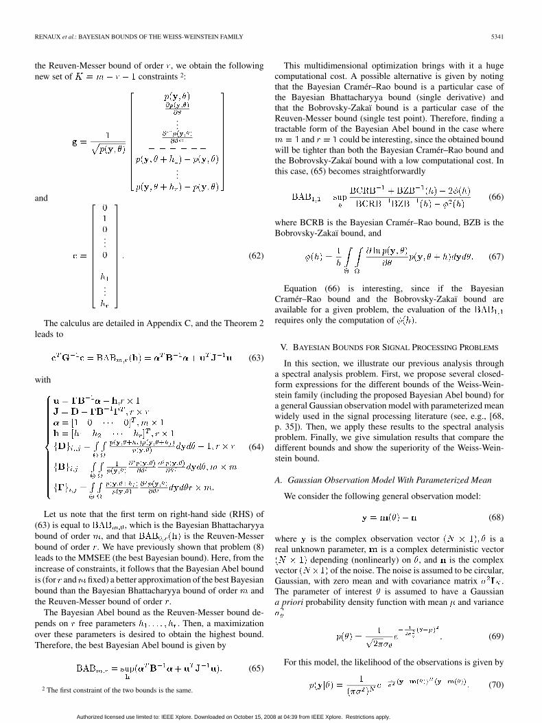
The calculus are detailed in Appendix C, and the Theorem 2leads to

(63)

with

(64)

Let us note that the first term on right-hand side (RHS) of(63) is equal to , which is the Bayesian Bhattacharyyabound of order , and that is the Reuven-Messerbound of order . We have previously shown that problem (8)leads to the MMSEE (the best Bayesian bound). Here, from theincrease of constraints, it follows that the Bayesian Abel boundis (for and fixed) a better approximation of the best Bayesianbound than the Bayesian Bhattacharyya bound of order andthe Reuven-Messer bound of order .

The Bayesian Abel bound as the Reuven-Messer bound de-pends on free parameters . Then, a maximizationover these parameters is desired to obtain the highest bound.Therefore, the best Bayesian Abel bound is given by

(65)

2 The first constraint of the two bounds is the same.

This multidimensional optimization brings with it a hugecomputational cost. A possible alternative is given by notingthat the Bayesian Cramér–Rao bound is a particular case ofthe Bayesian Bhattacharyya bound (single derivative) andthat the Bobrovsky-Zakaï bound is a particular case of theReuven-Messer bound (single test point). Therefore, finding atractable form of the Bayesian Abel bound in the case where

and could be interesting, since the obtained boundwill be tighter than both the Bayesian Cramér–Rao bound andthe Bobrovsky-Zakaï bound with a low computational cost. Inthis case, (65) becomes straightforwardly

(66)

where BCRB is the Bayesian Cramér–Rao bound, BZB is theBobrovsky-Zakaï bound, and

(67)

Equation (66) is interesting, since if the BayesianCramér–Rao bound and the Bobrovsky-Zakaï bound areavailable for a given problem, the evaluation of therequires only the computation of .

V. BAYESIAN BOUNDS FOR SIGNAL PROCESSING PROBLEMS

In this section, we illustrate our previous analysis througha spectral analysis problem. First, we propose several closed-form expressions for the different bounds of the Weiss-Wein-stein family (including the proposed Bayesian Abel bound) fora general Gaussian observation model with parameterized meanwidely used in the signal processing literature (see, e.g., [68,p. 35]). Then, we apply these results to the spectral analysisproblem. Finally, we give simulation results that compare thedifferent bounds and show the superiority of the Weiss-Wein-stein bound.

A. Gaussian Observation Model With Parameterized Mean

We consider the following general observation model:

(68)

where is the complex observation vector is areal unknown parameter, is a complex deterministic vector

depending (nonlinearly) on , and is the complexvector of the noise. The noise is assumed to be circular,Gaussian, with zero mean and with covariance matrix .The parameter of interest is assumed to have a Gaussiana priori probability density function with mean and variance

(69)

For this model, the likelihood of the observations is given by

(70)



To the best of our knowledge, only the Cramér–Rao boundexpression is known in this case (see [68]).

The Bayesian Bhattacharyya bound requires the calculationof several derivatives of the joint probability function in orderto be significantly tighter than the Cramér–Rao bound, which isgenerally difficult (see [69, Ch. 4] for an example for which theBhattacharyya bound of order 2 requires much algebraic effortto finally be equal to the Cramér–Rao bound). Consequently, wewill not use this bound here.

The details are given in Appendix D.1) Bayesian Cramér–Rao Bound:

(71)

2) Bobrovsky-Zakaï Bound:

(72)

3) Bayesian Abel Bound: is given by (66):

(73)

where

(74)

and

(75)

4) Weiss-Weinstein Bound: We now consider the Weiss-Weinstein bound with one test point, which can be simplifiedas follows (see [42, eq. (6)]):

(76)

where the key point to evaluate this bound is , which isthe semi-invariant moment generating function [70], defined asfollows:

(77)

This function is given by (78), as shown at the bottom of thepage.

B. Spectral Analysis Problem

We now consider the following observation model involvedin spectral analysis:

(79)

where is the complex observation. The observationsare assumed to be independent. is the amplitude of thesingle cisoïde of frequency . is a sequence of randomvariables assumed complex, circular, i.i.d, Gaussian, with zeromean and variance . Consequently the SNR is given by

. The parameter of interest is the frequencywhich is a Gaussian random variable

with mean and variance (69).This model is a particular case of the model (68), where

(80)

with

(81)

Let . The likelihood of the observa-tion is given by

(82)

Note that, if is assumed to be deterministic and in a digitalcommunications context, some closed-form expressions of de-terministic bounds can be found in [56].

The details of the calculus for the Weiss-Weinstein family aregiven in Appendix E.

1) Cramér–Rao Bound:

(83)

2) Bobrovsky-Zakaï Bound:

(84)

3) Bayesian Abel Bound: The is given by (66)

(85)

(78)



where

(86)

and

(87)

4) Weiss-Weinstein Bound: The Weiss-Weinstein bound isgiven by

(88)

where is given by

(89)

The Weiss-Weinstein bound needs to be optimized over twocontinuous parameters, which creates significant computationalcost. Here, two methods for reducing the computational cost arepresented.

• As previously stated, is chosen on the parameter supportwhich is approximated by . This support can bereduced to , since the function is even with respectto . Note that this remark holds for the Bayesian Abelbound and the Bobrovsky-Zakaï bound.

• As proposed by Weiss and Weinstein in [42], it is some-times a good choice to set . This approximationis intuitively justified by the fact that the Weiss-Weinsteinbound tends to the Bobrovsky-Zakaï bound when tendsto zero or one. Unfortunately, no sound proof that this re-sult is true in general is available in the literature. If weset is modified as follows: [see (90) atthe bottom of the page] and the modified Weiss-Weinsteinbound becomes

(91)

The resulting bound has approximaely the same computa-tional cost as the BZB and the BAB.

Fig. 1. Comparison of the global MSE of the MLE and of the MAP estimator,the Cramér–Rao bound, the Bobrovsky-Zakaï bound, the Bayesian Abel bound,and the Weiss-Weinstein bound with optimization over s and s = 1=2.N = 15

observations. � = 1=36 rad .

C. Simulations

In order to illustrate our results on the different bounds,we present here a simulation result for the spectral analysisproblem.

We consider a scenario with observations and,without loss of generality, . The estimator will be themaximum likelihood estimator (MLE) given for this model by

(92)

We also use the maximum a posteriori (MAP) estimatorgiven by

(93)

The global MSE will be computed by using (3) and 1000Monte Carlo runs. For the a priori probability density functionof the parameter of interest, we choose andrad .

Fig. 1 superimposes the global MSE of the MLE and of theMAP estimator, the Cramér–Rao bound, the Bobrovsky-Zakaïbound, the Bayesian Abel bound, and the Weiss-Weinsteinbound with optimization over and .

(90)



This figure shows the threshold behavior of both estimatorswhen the SNR decreases. In contrast to the Cramér–Rao bound,the Bobrovsky-Zakaï bound, the Bayesian Abel bound, and theWeiss-Weinstein bound exhibit the threshold phenomena. TheBayesian Abel bound is slightly higher than the Bobrovsky-Zaka ï bound and, consequently, leads to a better predictionof the threshold effect with the same computational cost. TheWeiss-Weinstein bounds obtained by numerical evaluation of(88) and (91) are the same; therefore, seems to bethe optimum value in this problem. As expected by the addi-tion of constraints, the Weiss-Weinstein bounds provide a betterprediction of the global MSE of the estimators in comparisonwith the Bobrovsky-Zakaï bound and the Bayesian Abel bound.The Weiss-Weinstein bound threshold value provides a betterapproximation of the effective SNR at which the estimators ex-perience the threshold behavior.

VI. CONCLUSION

In this paper, we proposed a framework to study the Bayesianminimal bounds on the MSE of the Weiss-Weinstein family.This framework is based on both the best Bayesian bound(MMSE) and a constrained optimization problem. By rewritingthe problem of the MMSEE as a continuous constrained opti-mization problem and by relaxing these constraints, we reobtainthe lower bounds of the Weiss-Weinstein family. Moreover, thisframework allows us to propose new minimal bounds. In thisway, we propose an extension of the Bayesian Bhattacharyyabound and a Bayesian version of the Abel bound. Additionally,we give some closed-form expressions of several minimalbounds for both a general Gaussian observation model withparameterized mean and a spectral analysis model.

APPENDIX

A. Proof of Theorem 1

This proof is based on the three following lemmas.Lemma 1:

(94)

Lemma 2:

(95)

Lemma 3:

(96)

Proof of Lemma 1:• we assume that

S

S

Since

(97)

we have

(98)

(99)

Since (99) holds for any , if we choose, we obtain

(100)

where is a function of only.• : on the other hand, if we assume that

, then

(101)

These two items prove Lemma 1.Proof of Lemma 2:

• we assume that such thatand such that

(102)

Then, when , we have

(103)

thanks to the result of the first item of Lemma 1.



• on the other hand, if we assume, then by setting

(104)

leading to

(105)

such that and such

that .These two items prove Lemma 2.

Proof of Lemma 3:• : let and assume

that such that

such that and

(106)

Then, when , we obtain

(107)

thanks to the result of the first item of Lemma 2.• : on the other hand, if we assume

, then by letting

(108)

Fig. 2. Graphical representation of the problem.

leading to

(109)

such that such

that and .These two items prove Lemma 3.Lemmas 1, 2, and 3 prove Theorem 1.

B. Proof of Theorem 2

Let be a vector space of any dimension on the field of realnumbers , with an inner product denoted by , whereand are two vectors of . Let be a family ofindependent vectors of and be a vectorof . We are interested in the solution of the minimization of

subject to the following linear constraints.

Let be the vectorial subspace of dimension generatedby the elements . Then, ,where is the orthogonal projection of on , i.e., the vector

such that (see Fig. 2) fora graphical representation).

Let be the coordinates of in thebasis of (i.e., ). These coor-dinates satisfy: . Moreover, ifsatisfies the constraints , then

(110)

i.e., by a matricial rewriting , where is the Grammatrix associated to the family : .The equation has for unique solution . Let



be the vector of corresponding to this solution. Then,and for satisfying the aforementioned constraints

we have , andthe minimum is achieved for , which means that isthe solution of the problem. The value of the minimal norm isgiven by

(111)

C. Derivation of the Bayesian Abel Bound

We have to calculate the quadratic form (29). Since

(112)

and, due to (9)

(113)

the matrix can now be written as the fol-

lowing partitioned matrix:

(114)

where the elements and of the matricesand are given by (37) and (48), respectively, and

the element of the matrix is given by

(115)

Let and , where

(size ), and .Since the first element of is null, only the right bottom corner

(size ) of is of interest. isgiven straightforwardly by

(116)

Consequently, the Bayesian Abel bound denoted isthen given by

(117)

After some algebraic effort, we obtain the final form

(118)

with

(119)

D. Minimal Bounds Derivation for the Gaussian ObservationModel With Parameterized Mean

1) Bayesian Cramér–Rao Bound: The Bayesian Cramér–Rao bound can be divided into two terms [20]

(120)

where is the standard (i.e., deterministic) Cramér–Raobound given by [68]:

(121)

where is the true value of the parameter in the deterministiccontext.

The second term of (120) is

(122)

Consequently

(123)

2) Bobrovsky-Zakaï Bound: The Bobrovsky-Zakaï bound isgiven by

(124)



The double integral in the last equation can be rewritten asfollows:

(125)

The term becomes (126), shown at thebottom of the page.

Let , and note that

Consequently [see (127) at the bottom of the page].The Bobrovsky-Zakaï bound is finally given by

(128)

3) Bayesian Abel Bound: We have to calculate

(129)

The first term in (129) is given by

(130)

For the second term in (129), we have

(131)

(126)

(127)



Finally

(132)

4) Weiss-Weinstein Bound: We have to calculate

(133)

This function can be modified as follows:

(134)

Let us first study the term shown in (135) at the bottom of thepage.

Let . Note that

(136)

Consequently, [see (137) at the bottom of the page].For the second term

(138)

Finally, the semi-invariant moment generating function isgiven by (139), shown at the bottom of the page.

E. Bayesian Bounds Derivation for a Spectral AnalysisProblem

1) Cramér–Rao Bound: The Bayesian Cramér–Rao boundis given by (123)

(140)

The term can be written

(141)

which is independent of . Consequently, the BayesianCramér–Rao bound is

(142)

(135)

(137)

(139)



2) Bobrovsky-Zakaï Bound: The Bobrovsky-Zakaï bound isgiven by (128)

(143)

In the case of our specific model (79), the termcan be written

(144)

which is independent of . The term

becomes

(145)

where the term is given by [71, p.

355, eq. (BI (28) (1))]

(146)

Finally, the Bobrovsky-Zakaï is given by

(147)

3) Bayesian Abel Bound: We have to calculate (132)

(148)

The term can berewritten as follows:

(149)

which is independent of . Consequently

(150)

4) Weiss-Weinstein Bound: We have to calculate (139)

(151)

thanks to (144) and to the independence of in the term.

The remaining term is given by

(152)

where is obtained thanks to [71, p.

355, eq. (BI(28)(1))].Consequently, is given by

(153)

ACKNOWLEDGMENT

This paper was developed while A. Renaux was a Post-doctoral Research Associate in Prof. Nehorai’s research groupat the Department of Electrical and Systems Engineering,Washington University, St. Louis.



REFERENCES

[1] A. Renaux, P. Forster, and P. Larzabal, “A new derivation of theBayesian bounds for parameter estimation,” in Proc. IEEE Statist.Signal Process. Workshop—SSP05, Bordeaux, France, Jul. 2005, pp.567–572.

[2] A. Renaux, P. Forster, P. Larzabal, and C. Richmond, “The BayesianAbel bound on the mean square error,” in Proc. IEEE Int. Conf. Acoust.,Speech, Signal Process., Toulouse, France, May 2006, vol. 3, pp. 9–12.

[3] R. A. Fisher, “On the mathematical foundations of theoretical statis-tics,” Phil. Trans. Royal Soc., vol. 222, p. 309, 1922.

[4] D. Dugué, “Application des propriétés de la limite au sens du calculdes probabilités à I’étude des diverses questions d’estimation,” Ecol.Poly., vol. 3, pp. 305–372, 1937.

[5] M. Frechet, “Sur I’extension de certaines evaluations statistiques ancas de petit echantillons,” Rev. Inst. Int. Statist., vol. 11, pp. 182–205,1943.

[6] G. Darmois, “Sur les lois limites de la dispersion de certaines estima-tions,” Rev. Inst. Int. Statist., vol. 13, pp. 9–15, 1945.

[7] C. R. Rao, “Information and accuracy attainable in the estimation ofstatistical parameters,” Bull. Calcutta Math. Soc., vol. 37, pp. 81–91,1945.

[8] H. Cramér, Mathematical Methods of Statistics. New York: PrincetonUniv. Press, 1946.

[9] L. L. Scharf and T. McWhorter, “Geometry of the Cramer Rao bound,”Signal Process., vol. 31, pp. 301–311, 1993.

[10] J. Xavier and V. Barroso, “The Riemannian geometry of certain param-eter estimation problems with singular Fisher information matrices,”in Proc. IEEE Int. Conf. Acoust., Speech, Signal Process., Montreal,Canada, May 2004, vol. 2, pp. 1021–1024.

[11] J. Xavier and V. Barroso, “Intrinsic variance lower bound (IVLB): Anextension of the Cramer Rao bound to Riemannian manifolds,” in Proc.IEEE Int. Conf. Acoust., Speech, Signal Process., Hong Kong, Mar.2004, vol. 5, pp. 1033–1036.

[12] A. Manikas, Differential Geometry in Array Processing. London,U.K.: Imperial College Press, 2004.

[13] S. T. Smith, “Statistical resolution limits and the complexified CramerRao bound,” IEEE Trans. Signal Process., vol. 53, pp. 1597–1609, May2005.

[14] S. T. Smith, “Covariance, subspace, and intrinsic Cramer Rao bounds,”IEEE Trans. Signal Process., vol. 53, pp. 1610–1630, May 2005.

[15] J.-P. Delmas and H. Abeida, “Stochastic Cramer-Rao bound for noncir-cular signals with application to DOA estimation,” IEEE Trans. SignalProcess., vol. 52, pp. 3192–3199, Nov. 2004.

[16] J.-P. Delmas and H. Abeida, “Cramer Rao bounds of DOA estimatesfor BPSK and QPSK modulated signals,” IEEE Trans. Signal Process.,vol. 54, pp. 117–126, Jan. 2005.

[17] E. Chaumette, P. Larzabal, and P. Forster, “On the influence of a de-tection step on lower bounds for deterministic parameter estimation,”IEEE Trans. Signal Process., vol. 53, pp. 4080–4090, Nov. 2005.

[18] Q. Zou, Z. Lin, and R. J. Ober, “The Cramer Rao lower bound forbilinear systems,” IEEE Trans. Signal Process., vol. 54, pp. 1666–1680,May 2006.

[19] I. Yetik and A. Nehorai, “Performance bounds on image registration,”IEEE Trans. Signal Process., vol. 54, pp. 1737–1736, May 2006.

[20] H. L. Van Trees, Detection, Estimation and Modulation Theory. NewYork: Wiley, 1968, vol. 1.

[21] D. C. Rife and R. R. Boorstyn, “Single tone parameter estimationfrom discrete time observations,” IEEE Trans. Inf. Theory, vol. 20, pp.591–598, 1974.

[22] A. Bhattacharyya, “On some analogues of the amount of informationand their use in statistical estimation,” Sankhya Indian J. Statist., vol.8, pp. 1–14, 201–218, 315–328, 1946.

[23] D. A. S. Fraser and I. Guttman, “Bhattacharyya bounds without regu-larity assumptions,” Ann. Math. Stat., vol. 23, pp. 629–632, 1952.

[24] D. G. Chapman and H. Robbins, “Minimum variance estimationwithout regularity assumptions,” Ann. Math. Stat., vol. 22, pp.581–586, 1951.

[25] J. Kiefer, “On minimum variance estimators,” Ann. Math. Stat., vol. 23,pp. 627–629, 1952.

[26] J. M. Hammersley, “On estimating restricted parametrers,” J. RoyalSoc. Ser. B, vol. 12, pp. 192–240, 1950.

[27] E. W. Barankin, “Locally best unbiased estimates,” Ann. Math. Stat.,vol. 20, pp. 477–501, 1949.

[28] R. J. McAulay and L. P. Seidman, “A useful form of the Barankin lowerbound and its application to ppm threshold analysis,” IEEE Trans. Inf.Theory, vol. 15, pp. 273–279, Mar. 1969.

[29] J. S. Abel, “A bound on mean square estimate error,” in Proc. IEEE Int.Conf. Acoust., Speech, Signal Process., Albuquerque, NM, 1990, vol.3, pp. 1345–1348.

[30] J. S. Abel, “A bound on mean square estimate error,” IEEE Trans. Inf.Theory, vol. 39, pp. 1675–1680, Sep. 1993.

[31] R. J. McAulay and E. M. Hofstetter, “Barankin bounds on parameterestimation,” IEEE Trans. Inf. Theory, vol. 17, pp. 669–676, Nov. 1971.

[32] A. Quinlan, E. Chaumette, and P. Larzabal, “A direct method to gen-erate approximations of the Barankin bound,” in Proc. IEEE Int. Conf.Acoust., Speech, Signal Process., Toulouse, France, May 2006, vol. 3,pp. 808–811.

[33] J. Ziv and M. Zakai, “Some lower bounds on signal parameter estima-tion,” IEEE Trans. Inf. Theory, vol. 15, pp. 386–391, May 1969.

[34] S. Bellini and G. Tartara, “Bounds on error in signal parameter estima-tion,” IEEE Trans. Commun., vol. 22, pp. 340–342, Mar. 1974.

[35] D. Chazan, M. Zakai, and J. Ziv, “Improved lower bounds on signalparameter estimation,” IEEE Trans. Inf. Theory, vol. 21, pp. 90–93,Jan. 1975.

[36] E. Weinstein, “Relations between Belini-Tartara, Chazan-Zakai-Ziv,and Wax-Ziv lower bounds,” IEEE Trans. Inf. Theory, vol. 34, pp.342–343, Mar. 1988.

[37] K. L. Bell, Y. Steinberg, Y. Ephraim, and H. L. V. Trees, “ExtendedZiv Zakai lower bound for vector parameter estimation,” IEEE Trans.Signal Process., vol. 43, pp. 624–638, Mar. 1997.

[38] K. L. Bell, “Performance bounds in parameter estimation with appli-cation to bearing estimation,” Ph.D. dissertation, George Mason Univ.,Fairfax, VA, 1995.

[39] B. Z. Bobrovsky, E. Mayer-Wolf, and M. Zakai, “Some classes ofglobal Cramer Rao bounds,” Ann. Statist., vol. 15, pp. 1421–1438,1987.

[40] B. Z. Bobrovsky and M. Zakai, “A lower bound on the estimation errorfor certain diffusion processes,” IEEE Trans. Inf. Theory, vol. 22, pp.45–52, Jan. 1976.

[41] I. Reuven and H. Messer, “A Barankin-type lower bound on the esti-mation error of a hybrid parameter vector,” IEEE Trans. Inf. Theory,vol. 43, no. 3, pp. 1084–1093, May 1997.

[42] A. J. Weiss and E. Weinstein, “A lower bound on the mean square errorin random parameter estimation,” IEEE Trans. Inf. Theory, vol. 31, pp.680–682, Sep. 1985.

[43] , H. L. Van Trees and K. L. Bell, Eds., Bayesian Bounds for Param-eter Estimation and Nonlinear Filtering/Tracking. New York: Wiley,2007.

[44] A. B. Baggeroer, Barankin Bound on the Variance of Estimates ofGaussian Random Process MIT Lincoln Lab., Lexington, MA, Tech.Rep., Jan. 1969.

[45] I. Reuven and H. Messer, “The use of the Barankin bound for deter-mining the threshold SNR in estimating the bearing of a source in thepresence of another,” in Proc. IEEE Int. Conf. Acoust., Speech, SignalProcess., Detroit, MI, May 1995, vol. 3, pp. 1645–1648.

[46] L. Knockaert, “The Barankin bound and threshold behavior infrequency estimation,” IEEE Trans. Signal Process., vol. 45, pp.2398–2401, Sep. 1997.

[47] J. Tabrikian and J. L. Krolik, “Barankin bound for source localizationin shallow water,” in Proc. IEEE Int. Conf. Acoust., Speech, SignalProcess., Munich, Germany, Apr. 1997.

[48] T. L. Marzetta, “Computing the Barankin bound by solving an un-constrained quadratic optimization problem,” in Proc. IEEE Int. Conf.Acoust., Speech, Signal Process., Munich, Germany, Apr. 1997, vol. 5,pp. 3829–3832.

[49] I. Reuven and H. Messer, “On the effect of nuisance parameters onthe threshold SNR value of the Barankin bound,” IEEE Trans. SignalProcess., vol. 47, no. 2, pp. 523–527, Feb. 1999.

[50] J. Tabrikian and J. Krolik, “Barankin bounds for source localization inan uncertain ocean environment,” IEEE Trans. Signal Process., vol. 47,pp. 2917–2927, Nov. 1999.

[51] A. Ferrari and J.-Y. Tourneret, “Barankin lower bound for changepoints in independent sequences,” in Proc. IEEE Statist. SignalProcess. Workshop—SSP03, St. Louis, MO, Sep. 2003, pp. 557–560.

[52] P. Ciblat, M. Ghogho, P. Forster, and P. Larzabal, “Harmonic retrievalin the presence of non-circular Gaussian multiplicative noise: Perfor-mance bounds,” Signal Process., vol. 85, pp. 737–749, Apr. 2005.

[53] P. Ciblat, P. Forster, and P. Larzabal, “Harmonic retrieval in noncir-cular complex-valued multiplicative noise: Barankin bound,” in Proc.EUS1PCO, Vienne, Australia, Sep. 2004, pp. 2151–2154.

[54] L. Atallah, J. P. Barbot, and P. Larzabal, “SNR threshold indicator indata aided frequency synchronization,” IEEE Signal Process. Lett., vol.11, pp. 652–654, Aug. 2004.



[55] L. Atallah, J. P. Barbot, and P. Larzabal, “From Chapman Robbinsbound towards Barankin bound in threshold behavior prediction,” Elec-tron. Lett., vol. 40, pp. 279–280, Feb. 2004.

[56] A. Renaux, L. N. Atallah, P. Forster, and P. Larzabal, “A useful form ofthe Abel bound and its application to estimator threshold prediction,”IEEE Trans. Signal Process., vol. 55, no. 5, pp. 2365–2369, May 2007.

[57] W. Xu, “Performances bounds on matched-field methods for sourcelocalization and estimation of ocean environmental parameters,” Ph.D.dissertation, Mass. Inst. Technol., Cambridge, Jun. 2001.

[58] W. Xu, A. B. Baggeroer, and K. Bell, “A bound on mean-squareestimation with background parameter mismatch,” IEEE Trans. Inf.Theory, vol. 50, pp. 621–632, Apr. 2004.

[59] W. Xu, A. B. Baggeroer, and C. D. Richmond, “Bayesian bounds formatched-field parameter estimation,” IEEE Trans. Signal Process., vol.52, pp. 3293–3305, Dec. 2004.

[60] A. J. Weiss and E. Weinstein, “Fundamental limitation in passive timedelay estimation Part 1: Narrowband systems,” IEEE Trans. Acoust.,Speech, Signal Process., vol. 31, pp. 472–486, Apr. 1983.

[61] K. L. Bell, Y. Ephraim, and H. L. V. Trees, “Ziv Zakai lower bounds inbearing estimation,” in Proc. IEEE Int. Conf. Acoust., Speech, SignalProcess., Detroit, MI, 1995, vol. 5, pp. 2852–2855.

[62] K. L. Bell, Y. Ephraim, and H. L. V. Trees, “Explicit Ziv Zakai lowerbound for bearing estimation,” IEEE Trans. Signal Process., vol. 44,pp. 2810–2824, Nov. 1996.

[63] P. Ciblat and M. Ghogho, “Ziv Zakai bound for harmonic retrievalin multiplicative and additive Gaussian noise,” in Proc. IEEE Statist.Signal Process. Workshop—SSP05, Bordeaux, France, Jul. 2005, pp.561–566.

[64] A. Renaux, “Weiss-Weinstein bound for data aided carrier estimation,”IEEE Signal Process. Lett., vol. 14, no. 4, pp. 283–286, Apr. 2007.

[65] F. E. Glave, “A new look at the Barankin lower bound,” IEEE Trans.Inf. Theory, vol. 18, no. 3, pp. 349–356, May 1972.

[66] P. Forster and P. Larzabal, “On lower bounds for deterministic pa-rameter estimation,” in Proc. IEEE Int. Conf. Acoust., Speech, SignalProcess., Orlando, FL, 2002, vol. 2, pp. 1137–1140.

[67] E. Weinstein and A. J. Weiss, “A general class of lower bounds in pa-rameter estimation,” IEEE Trans. Inf. Theory, vol. 34, pp. 338–342,Mar. 1988.

[68] S. M. Kay, Fundamentals of Statistical Signal Processing. Engle-wood Cliffs, NJ: Prentice-Hall, 1993, vol. I.

[69] A. Renaux, “Contribution a panalyse des performances d’estimaiionen traitement statisticue du signal” Ph.D. dissertation, Ecole NormaleSuperieure de Cachan, Cachan, France, Jul. 2006 [Online]. Available:http://www.satie.ens-c;achan.fr/ts/These_Alex.pdf

[70] H. L. Van Trees, Detection, Estimation and Modulation Theory: Radar-Sonar Signal Processing and Gaussian Signals in Noise. New York:Wiley, 2001, vol. 3.

[71] S. Gradshteyn and I. M. Ryzhik, Table of Integrals, Series, and Prod-ucts. San Diego, CA: Academic, 1994.

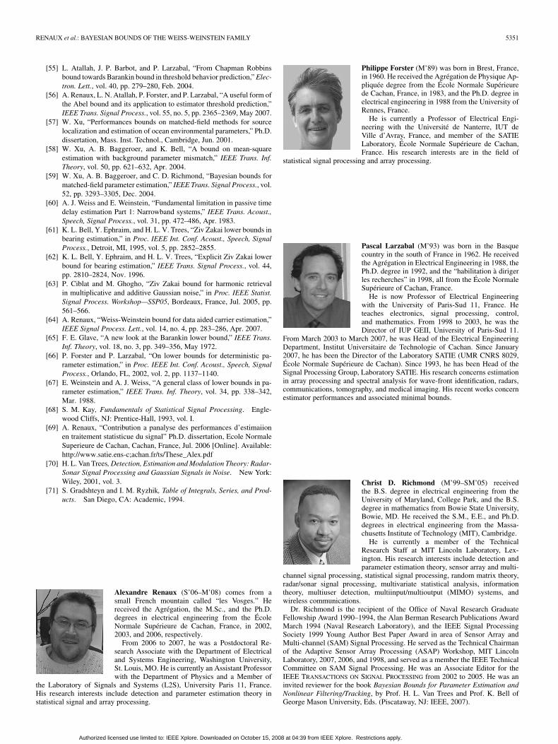
Alexandre Renaux (S’06–M’08) comes from asmall French mountain called “les Vosges.” Hereceived the Agrégation, the M.Sc., and the Ph.D.degrees in electrical engineering from the ÉcoleNormale Supérieure de Cachan, France, in 2002,2003, and 2006, respectively.

From 2006 to 2007, he was a Postdoctoral Re-search Associate with the Department of Electricaland Systems Engineering, Washington University,St. Louis, MO. He is currently an Assistant Professorwith the Department of Physics and a Member of

the Laboratory of Signals and Systems (L2S), University Paris 11, France.His research interests include detection and parameter estimation theory instatistical signal and array processing.

Philippe Forster (M’89) was born in Brest, France,in 1960. He received the Agrégation de Physique Ap-pliquée degree from the École Normale Supérieurede Cachan, France, in 1983, and the Ph.D. degree inelectrical engineering in 1988 from the University ofRennes, France.

He is currently a Professor of Electrical Engi-neering with the Université de Nanterre, IUT deVille d’Avray, France, and member of the SATIELaboratory, École Normale Supérieure de Cachan,France. His research interests are in the field of

statistical signal processing and array processing.

Pascal Larzabal (M’93) was born in the Basquecountry in the south of France in 1962. He receivedthe Agrégation in Electrical Engineering in 1988, thePh.D. degree in 1992, and the “habilitation à dirigerles recherches” in 1998, all from the École NormaleSupérieure of Cachan, France.

He is now Professor of Electrical Engineeringwith the University of Paris-Sud 11, France. Heteaches electronics, signal processing, control,and mathematics. From 1998 to 2003, he was theDirector of IUP GEII, University of Paris-Sud 11.

From March 2003 to March 2007, he was Head of the Electrical EngineeringDepartment, Institut Universitaire de Technologie of Cachan. Since January2007, he has been the Director of the Laboratory SATIE (UMR CNRS 8029,École Normale Supérieure de Cachan). Since 1993, he has been Head of theSignal Processing Group, Laboratory SATIE. His research concerns estimationin array processing and spectral analysis for wave-front identification, radars,communications, tomography, and medical imaging. His recent works concernestimator performances and associated minimal bounds.

Christ D. Richmond (M’99–SM’05) receivedthe B.S. degree in electrical engineering from theUniversity of Maryland, College Park, and the B.S.degree in mathematics from Bowie State University,Bowie, MD. He received the S.M., E.E., and Ph.D.degrees in electrical engineering from the Massa-chusetts Institute of Technology (MIT), Cambridge.

He is currently a member of the TechnicalResearch Staff at MIT Lincoln Laboratory, Lex-ington. His research interests include detection andparameter estimation theory, sensor array and multi-

channel signal processing, statistical signal processing, random matrix theory,radar/sonar signal processing, multivariate statistical analysis, informationtheory, multiuser detection, multiinput/multioutput (MIMO) systems, andwireless communications.

Dr. Richmond is the recipient of the Office of Naval Research GraduateFellowship Award 1990–1994, the Alan Berman Research Publications AwardMarch 1994 (Naval Research Laboratory), and the IEEE Signal ProcessingSociety 1999 Young Author Best Paper Award in area of Sensor Array andMulti-channel (SAM) Signal Processing. He served as the Technical Chairmanof the Adaptive Sensor Array Processing (ASAP) Workshop, MIT LincolnLaboratory, 2007, 2006, and 1998, and served as a member the IEEE TechnicalCommittee on SAM Signal Processing. He was an Associate Editor for theIEEE TRANSACTIONS ON SIGNAL PROCESSING from 2002 to 2005. He was aninvited reviewer for the book Bayesian Bounds for Parameter Estimation andNonlinear Filtering/Tracking, by Prof. H. L. Van Trees and Prof. K. Bell ofGeorge Mason University, Eds. (Piscataway, NJ: IEEE, 2007).



Arye Nehorai (S’80–M’83–SM’90–F’94) receivedthe B.Sc. and M.Sc. degrees in electrical engineeringfrom the Technion, Israel, and the Ph.D. degreein electrical engineering from Stanford University,Stanford, CA.

From 1985 to 1995, he was a faculty memberwith the Department of Electrical Engineering, YaleUniversity, New Haven, CT. In 1995, he joined theDepartment of Electrical Engineering and ComputerScience, The University of Illinois at Chicago (UIC)as Full Professor. From 2000 to 2001, he was Chair

of the department’s Electrical and Computer Engineering (ECE) Division,which then became a new department. In 2001, he was named UniversityScholar of the University of Illinois. In 2006, he became Chairman of theDepartment of Electrical and Systems Engineering, Washington University, St.Louis (WUSTL), MO. He is the inaugural holder of the Eugene and Martha

Lohman Professorship and the Director of the Center for Sensor Signal andInformation Processing (CSSIP) at WUSTL since 2006.

Dr. Nehorai was Editor-in-Chief of the IEEE TRANSACTIONS ON SIGNAL

PROCESSING during 2000 to 2002. During 2003–2005, he was Vice President(Publications) of the IEEE Signal Processing Society, Chair of the PublicationsBoard, member of the Board of Governors, and member of the Executive Com-mittee of this Society. From 2003 to 2006, he was the Founding Editor of theSpecial Columns on Leadership Reflections in the IEEE SIGNAL PROCESSING

MAGAZINE. He was corecipient of the IEEE SPS 1989 Senior Award for BestPaper with P. Stoica, coauthor of the 2003 Young Author Best Paper Award,and corecipient of the 2004 Magazine Paper Award with A. Dogandzic. He waselected Distinguished Lecturer of the IEEE SPS for the term 2004 to 2005 andreceived the 2006 IEEE SPS Technical Achievement Award. He is the PrincipalInvestigator of the new multidisciplinary university research initiative (MURI)project entitled Adaptive Waveform Diversity for Full Spectral Dominance. Hehas been a Fellow of the Royal Statistical Society since 1996.


Documents

A Fresh Look at the Bayesian Bounds of the Weiss-Weinstein Family