Embed Size (px)
Citation preview
Computational bounds on polynomial
differential equations
Daniel S. Graca a,b , Jorge Buescu c,d ,Manuel L. Campagnolo e,b ,
aDM/FCT da Universidade do Algarve, PortugalbSQIG/Instituto de Telecomunicacoes, Lisboa, Portugal
cDM/FCUL, University of Lisbon, PortugaldCMAF, Lisbon, Portugal
eDM/ISA, Technical University of Lisbon, Portugal
Abstract
In this paper we study from a computational perspective some properties of thesolutions of polynomial ordinary differential equations.
We consider elementary (in the sense of Analysis) discrete-time dynamical sys-tems satisfying certain criteria of robustness. We show that those systems can besimulated with elementary and robust continuous-time dynamical systems whichcan be expanded into fully polynomial ordinary differential equations in Q[π]. Thissets a computational lower bound on polynomial ODEs since the former class islarge enough to include the dynamics of arbitrary Turing machines.
We also apply the previous methods to show that the problem of determiningwhether the maximal interval of definition of an initial-value problem defined withpolynomial ODEs is bounded or not is in general undecidable, even if the parametersof the system are computable and comparable and if the degree of the correspondingpolynomial is at most 56.
Combined with earlier results on the computability of solutions of polynomialODEs, one can conclude that there is from a computational point of view a closeconnection between these systems and Turing machines.
Email addresses: [email protected] (Daniel S. Graca), [email protected](Jorge Buescu), [email protected] (Manuel L. Campagnolo).
Preprint submitted to Elsevier 5 July 2008
1 Introduction
Differential equations are a powerful tool to model a diversity of phenomenain fields ranging from basic natural sciences like physics, chemistry or biologyto social sciences or economics. Among these, initial value problems (IVPs)of the form x′ = f(t, x), with x(t0) = x0, where f is a vector field and t isthe independent variable, play a predominant role. In this paper we considerthe large class of polynomial IVPs (PIVPs for short) in which f is a vector ofpolynomials. Many well known models, like the Lorenz equations in meteorol-ogy, the Lotka-Volterra equations for predator-prey systems, or Van der Pol’sequation in electronics [1] fall into this category. In Section 2 we show that infact all the elementary functions of Analysis are solutions of PIVPs. This is astronger version of the well established fact that all elementary functions aredifferentially algebraic [2]. It is also worth noticing that the solutions of PIVPsare precisely the set of functions definable with Shannon’s General PurposeAnalog Computer (GPAC) [3] as proved in [4].
While the qualitative behavior of linear systems (i. e. where f is linear) andplanar systems (where f : R3 → R2) is completely understood [5], it is notknown for all but a few cases how to predict the behavior of the solutionsof general PIVPs from the expression of f , which is the reason why manyfundamental questions about PIVPs (e.g. Hilbert’s 16th problem) are stillopen.
Since most nonlinear differential equations cannot be solved exactly, one hasto resort to numerical methods to obtain approximate solutions. This leads toa range of questions about computational properties of PIVPs. In particular,one can ask if PIVPs have computable approximations, if the domain of thesolution is computable, or even if deciding whether the maximal interval ofexistence is bounded is computable. Such questions have been answered foranalytic IVPs (where f is analytic) in [6]. In Section 2 we point out that theresults in [6] imply that the domain of existence of PIVP functions (i.e. so-lutions of PIVPs) is in general recursively enumerable and that the solutionis computable on its domain. This last result sets an upper bound on thecomputability of PIVP functions since it ensures that as long as f is polyno-mial and computable they can be arbitrarily approximated wherever they aredefined.
To obtain computational lower bounds for PIVPs, one can show that anycomputable function can be approximated by some PIVP function. In [7] itwas proved that under a simple (and unbounded) encoding in N3, the evolutionof Turing machines can be simulated with PIVPs. In this paper, we extendthat result and show that any computable discrete dynamical system on Nm
which admits a robust extension (to be defined) can be simulated with a PIVP.
2
The iteration of maps with IVPs is not new and can be found, for instance, in[8], [9]. However, those constructions are in some sense not satisfactory sincethey involve functions with some degree of discreteness (e.g. functions whichare not analytic or even have discontinuous derivatives) which can be used tobuild “exact clocks” that simulate the discrete steps of the iteration.
In Sections 3 and 4 we state and prove the main result of the paper. We showthat given a map ω on Nm, one can construct a PIVP with coefficients in Q[π]that simulates the iteration of ω as long as ω is extendable to a “robust” map Ωon Rm, in a sense to be defined in Section 3, and Ω is composition of polynomialand PIVP functions with parameters in Q[π] . The simulation is robust, whichis a necessity for our construction, but is also a natural requirement for acontinuous-time physical system described by an IVP. The constructions inSection 4 will also provide the necessary tools to address the issues discussedin the remainder of the paper.
Finally, in Section 5, we review and extend some undecidability results onPIVPs. Our results in [7] imply that reachability for PIVPs is undecidable,i.e., given a PIVP and some open set in phase space, there is no algorithm todecide if the solution of the PIVP crosses the open set. This contrasts with thedecidability of the reachability for linear differential equations [10]. In [11] weshowed that the boundedness of the domain of existence for PVIPs is undecid-able as long as f is polynomial of sufficiently high degree and computable. Atfirst sight, this result might seem trivial, since one can easily construct simplePIVPs which, upon varying one parameter, exhibit a critical value where thesolution is bounded on the left of this parameter value and unbounded on theright. For instance, the PIVP x′ = α(x2−1)t, x(0) = 3 has a maximal intervalwhich is bounded for α > 0 and unbounded if α ≤ 0. Since we cannot compareexactly two arbitrary computable reals [12] the boundedness problem for thePIVP above is undecidable. However, in Section 5 we show that if we con-sider that all input parameters are “comparable”, the boundedness problemremains undecidable. We also prove the claim in [11] that those undecidabilityresults hold for PIVPs where the degree of the polynomial is less or equal to56.
2 The GPAC, Polynomial Differential Equations, and ComputableAnalysis
In this section we introduce some useful definitions and results that will laterbe used in this paper.
Definition 1 Let I ⊆ R be a non-empty open interval and let t0 ∈ I. We saythat g : I → R is a PIVP function on I if it is a component of the solution of
3
the initial-value problem
x′ = p(t, x), x(t0) = x0 (1)
where p is a vector of polynomials and t0 ∈ I. We say that g is a PIVPfunction with parameters in S ⊆ R if the coefficients of p in (1), t0, and thecomponents of x0 belong to S.
Similarly we say that a function g : I ⊆ R→ Rk is a vector PIVP function ifeach component of g is a PIVP function.
Example 2 The following are examples of PIVP functions with parametersin Z: the exponential function ex, the trigonometric functions cos, sin [7], theinverse function x 7→ 1/x (solution of y′ = −y2; on (0,+∞) it can be obtainedby setting the initial condition y(1) = 1).
The PIVP functions are also closed under the following operations (as far aswe know, these properties have only been reported in the literature for thebroader case of differentially algebraic functions):
(1) Field operations +,−,×, /. For instance, if f, g : I → R, where I ⊆ R isan open interval, are PIVP functions, then so is f + g in I. In fact, if f, gare the first components of the solutions of the (vector) PIVPs
x′ = p(t, x)
x(t0) = x0
and
y′ = q(t, y)
y(t0) = y0
respectively then, since f ′(t) + g′(t) = p1(t, x) + q1(t, x), where p1(t, x)and q1(t, x) are the first components of p(t, x) and q(t, x) respectively,f + g is the last component of the solution of the PIVP
x′ = p(t, x)
y′ = q(t, y)
z′ = p1(t, x) + q1(t, y)
x(t0) = x0
y(t0) = y0
z(t0) = x0,1 + y0,1
where x0,1 and y0,1 are the first components of vectors x0 and y0, respec-tively. Similar proofs apply for the operations −,×, /. It should be notedthat the quotient f/g is a PIVP function in intervals which do not containzeros of g, and that the PIVP which generates f/g is well-defined in suchintervals. For instance tan(= sin
cos) is a PIVP function on (−π/2, π/2).
(2) Composition. If f : I → R, g : J → R, where I, J ⊆ R are open intervalsand f(I) ⊆ J , are PIVP functions, then so is g f on I. To see this,
4
suppose that f, g are the first components of the solutions of the PIVPsx′ = p(t, x)
x(t0) = x0
and
y′ = q(t, y)
y(t1) = y0
(2)
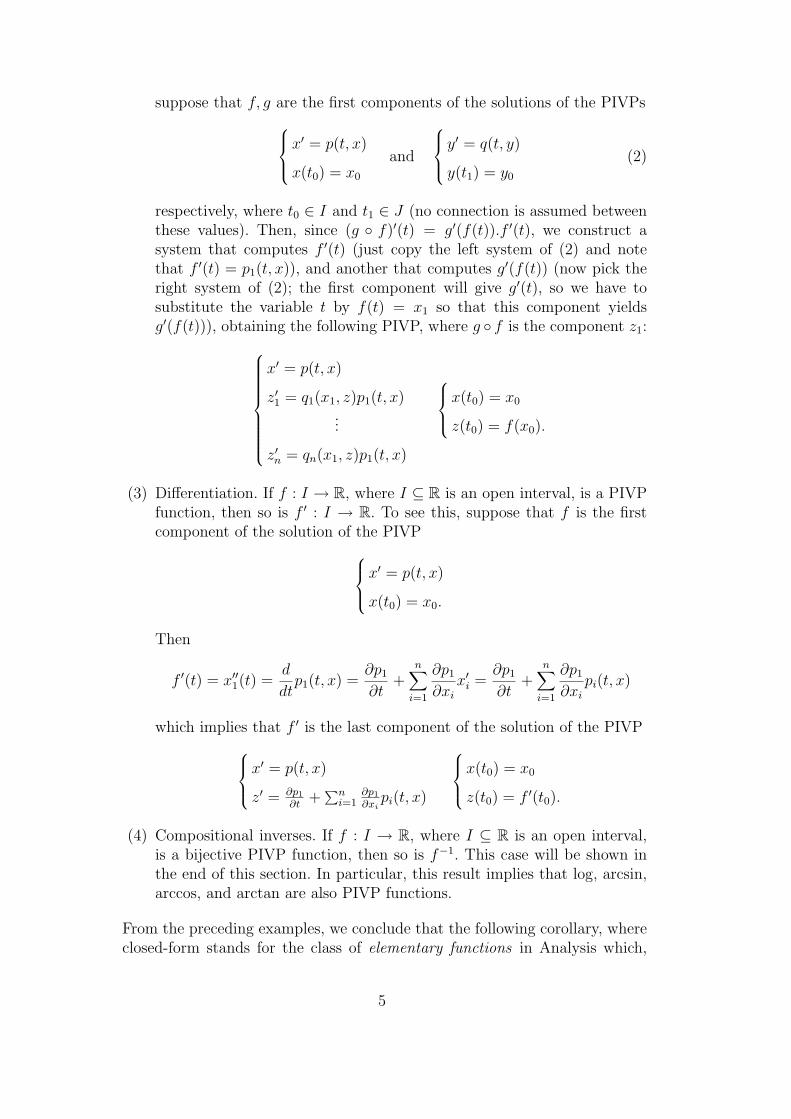
respectively, where t0 ∈ I and t1 ∈ J (no connection is assumed betweenthese values). Then, since (g f)′(t) = g′(f(t)).f ′(t), we construct asystem that computes f ′(t) (just copy the left system of (2) and notethat f ′(t) = p1(t, x)), and another that computes g′(f(t)) (now pick theright system of (2); the first component will give g′(t), so we have tosubstitute the variable t by f(t) = x1 so that this component yieldsg′(f(t))), obtaining the following PIVP, where g f is the component z1:
x′ = p(t, x)
z′1 = q1(x1, z)p1(t, x)...
z′n = qn(x1, z)p1(t, x)
x(t0) = x0
z(t0) = f(x0).
(3) Differentiation. If f : I → R, where I ⊆ R is an open interval, is a PIVPfunction, then so is f ′ : I → R. To see this, suppose that f is the firstcomponent of the solution of the PIVPx
′ = p(t, x)
x(t0) = x0.
Then
f ′(t) = x′′1(t) =d
dtp1(t, x) =
∂p1
∂t+
n∑i=1
∂p1
∂xix′i =
∂p1
∂t+
n∑i=1
∂p1
∂xipi(t, x)
which implies that f ′ is the last component of the solution of the PIVPx′ = p(t, x)
z′ = ∂p1∂t
+∑ni=1
∂p1∂xipi(t, x)
x(t0) = x0
z(t0) = f ′(t0).
(4) Compositional inverses. If f : I → R, where I ⊆ R is an open interval,is a bijective PIVP function, then so is f−1. This case will be shown inthe end of this section. In particular, this result implies that log, arcsin,arccos, and arctan are also PIVP functions.
From the preceding examples, we conclude that the following corollary, whereclosed-form stands for the class of elementary functions in Analysis which,
5
informally, correspond to the functions obtained from the rational functions,sin, cos, exp through finitely many compositions and inversions.
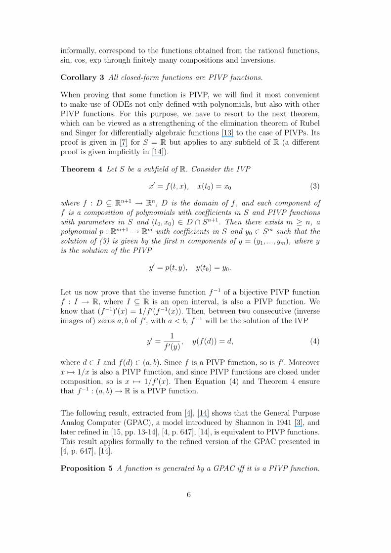
Corollary 3 All closed-form functions are PIVP functions.
When proving that some function is PIVP, we will find it most convenientto make use of ODEs not only defined with polynomials, but also with otherPIVP functions. For this purpose, we have to resort to the next theorem,which can be viewed as a strengthening of the elimination theorem of Rubeland Singer for differentially algebraic functions [13] to the case of PIVPs. Itsproof is given in [7] for S = R but applies to any subfield of R (a differentproof is given implicitly in [14]).
Theorem 4 Let S be a subfield of R. Consider the IVP
x′ = f(t, x), x(t0) = x0 (3)
where f : D ⊆ Rn+1 → Rn, D is the domain of f , and each component off is a composition of polynomials with coefficients in S and PIVP functionswith parameters in S and (t0, x0) ∈ D ∩ Sn+1. Then there exists m ≥ n, apolynomial p : Rm+1 → Rm with coefficients in S and y0 ∈ Sm such that thesolution of (3) is given by the first n components of y = (y1, ..., ym), where yis the solution of the PIVP
y′ = p(t, y), y(t0) = y0.
Let us now prove that the inverse function f−1 of a bijective PIVP functionf : I → R, where I ⊆ R is an open interval, is also a PIVP function. Weknow that (f−1)′(x) = 1/f ′(f−1(x)). Then, between two consecutive (inverseimages of) zeros a, b of f ′, with a < b, f−1 will be the solution of the IVP
y′ =1
f ′(y), y(f(d)) = d, (4)
where d ∈ I and f(d) ∈ (a, b). Since f is a PIVP function, so is f ′. Moreoverx 7→ 1/x is also a PIVP function, and since PIVP functions are closed undercomposition, so is x 7→ 1/f ′(x). Then Equation (4) and Theorem 4 ensurethat f−1 : (a, b)→ R is a PIVP function.
The following result, extracted from [4], [14] shows that the General PurposeAnalog Computer (GPAC), a model introduced by Shannon in 1941 [3], andlater refined in [15, pp. 13-14], [4, p. 647], [14], is equivalent to PIVP functions.This result applies formally to the refined version of the GPAC presented in[4, p. 647], [14].
Proposition 5 A function is generated by a GPAC iff it is a PIVP function.
6
Therefore, all results stated in this paper for PIVP functions are also valid forthe GPAC generable functions.
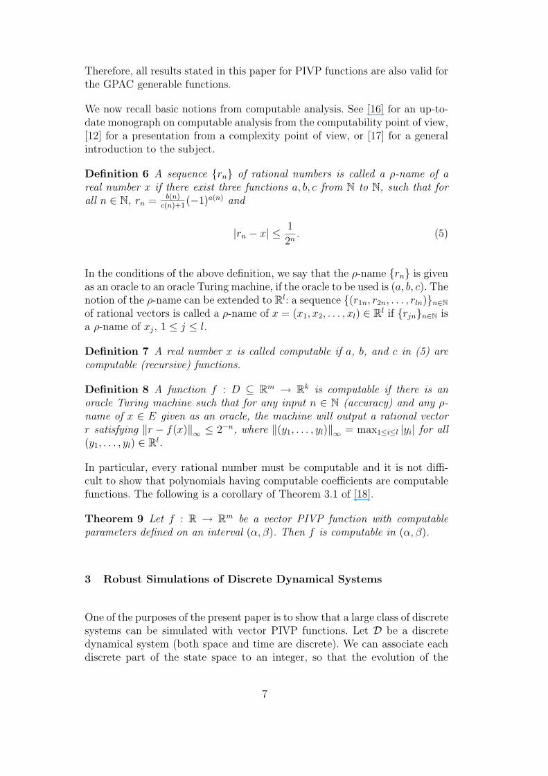
We now recall basic notions from computable analysis. See [16] for an up-to-date monograph on computable analysis from the computability point of view,[12] for a presentation from a complexity point of view, or [17] for a generalintroduction to the subject.
Definition 6 A sequence rn of rational numbers is called a ρ-name of areal number x if there exist three functions a, b, c from N to N, such that forall n ∈ N, rn = b(n)
c(n)+1(−1)a(n) and
|rn − x| ≤1
2n. (5)
In the conditions of the above definition, we say that the ρ-name rn is givenas an oracle to an oracle Turing machine, if the oracle to be used is (a, b, c). Thenotion of the ρ-name can be extended to Rl: a sequence (r1n, r2n, . . . , rln)n∈Nof rational vectors is called a ρ-name of x = (x1, x2, . . . , xl) ∈ Rl if rjnn∈N isa ρ-name of xj, 1 ≤ j ≤ l.
Definition 7 A real number x is called computable if a, b, and c in (5) arecomputable (recursive) functions.
Definition 8 A function f : D ⊆ Rm → Rk is computable if there is anoracle Turing machine such that for any input n ∈ N (accuracy) and any ρ-name of x ∈ E given as an oracle, the machine will output a rational vectorr satisfying ‖r − f(x)‖∞ ≤ 2−n, where ‖(y1, . . . , yl)‖∞ = max1≤i≤l |yi| for all(y1, . . . , yl) ∈ Rl.
In particular, every rational number must be computable and it is not diffi-cult to show that polynomials having computable coefficients are computablefunctions. The following is a corollary of Theorem 3.1 of [18].
Theorem 9 Let f : R → Rm be a vector PIVP function with computableparameters defined on an interval (α, β). Then f is computable in (α, β).
3 Robust Simulations of Discrete Dynamical Systems
One of the purposes of the present paper is to show that a large class of discretesystems can be simulated with vector PIVP functions. Let D be a discretedynamical system (both space and time are discrete). We can associate eachdiscrete part of the state space to an integer, so that the evolution of the
7
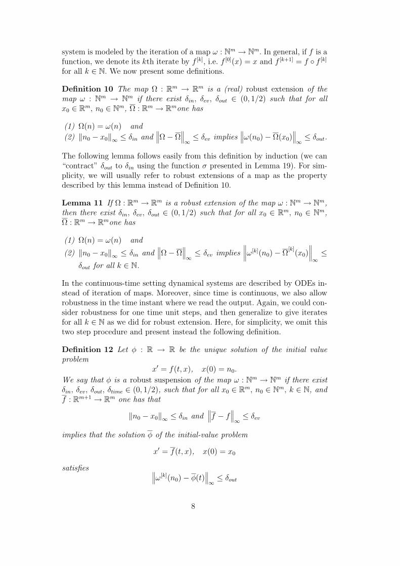
system is modeled by the iteration of a map ω : Nm → Nm. In general, if f is afunction, we denote its kth iterate by f [k], i.e. f [0](x) = x and f [k+1] = f f [k]
for all k ∈ N. We now present some definitions.
Definition 10 The map Ω : Rm → Rm is a (real) robust extension of themap ω : Nm → Nm if there exist δin, δev, δout ∈ (0, 1/2) such that for allx0 ∈ Rm, n0 ∈ Nm, Ω : Rm → Rmone has
(1) Ω(n) = ω(n) and
(2) ‖n0 − x0‖∞ ≤ δin and∥∥∥Ω− Ω
∥∥∥∞≤ δev implies
∥∥∥ω(n0)− Ω(x0)∥∥∥∞≤ δout.
The following lemma follows easily from this definition by induction (we can“contract” δout to δin using the function σ presented in Lemma 19). For sim-plicity, we will usually refer to robust extensions of a map as the propertydescribed by this lemma instead of Definition 10.
Lemma 11 If Ω : Rm → Rm is a robust extension of the map ω : Nm → Nm,then there exist δin, δev, δout ∈ (0, 1/2) such that for all x0 ∈ Rm, n0 ∈ Nm,Ω : Rm → Rmone has
(1) Ω(n) = ω(n) and
(2) ‖n0 − x0‖∞ ≤ δin and∥∥∥Ω− Ω
∥∥∥∞≤ δev implies
∥∥∥∥ω[k](n0)− Ω[k]
(x0)∥∥∥∥∞≤
δout for all k ∈ N.
In the continuous-time setting dynamical systems are described by ODEs in-stead of iteration of maps. Moreover, since time is continuous, we also allowrobustness in the time instant where we read the output. Again, we could con-sider robustness for one time unit steps, and then generalize to give iteratesfor all k ∈ N as we did for robust extension. Here, for simplicity, we omit thistwo step procedure and present instead the following definition.
Definition 12 Let φ : R → R be the unique solution of the initial valueproblem
x′ = f(t, x), x(0) = n0.
We say that φ is a robust suspension of the map ω : Nm → Nm if there existδin, δev, δout, δtime ∈ (0, 1/2), such that for all x0 ∈ Rm, n0 ∈ Nm, k ∈ N, andf : Rm+1 → Rm one has that
‖n0 − x0‖∞ ≤ δin and∥∥∥f − f∥∥∥
∞≤ δev
implies that the solution φ of the initial-value problem
x′ = f(t, x), x(0) = x0
satisfies ∥∥∥ω[k](n0)− φ(t)∥∥∥∞≤ δout
8
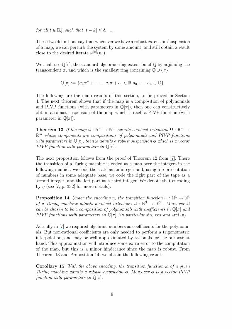
for all t ∈ R+0 such that |t− k| ≤ δtime.
These two definitions say that whenever we have a robust extension/suspensionof a map, we can perturb the system by some amount, and still obtain a resultclose to the desired iterate ω[k](n0).
We shall use Q[π], the standard algebraic ring extension of Q by adjoining thetranscendent π, and which is the smallest ring containing Q ∪ π:
Q[π] := anπn + . . .+ a1π + a0 ∈ R|a0, . . . , an ∈ Q.
The following are the main results of this section, to be proved in Section4. The next theorem shows that if the map is a composition of polynomialsand PIVP functions (with parameters in Q[π]), then one can constructivelyobtain a robust suspension of the map which is itself a PIVP function (withparameter in Q[π]).
Theorem 13 If the map ω : Nm → Nm admits a robust extension Ω : Rm →Rm whose components are compositions of polynomials and PIVP functionswith parameters in Q[π], then ω admits a robust suspension φ which is a vectorPIVP function with parameters in Q[π].
The next proposition follows from the proof of Theorem 12 from [7]. Therethe transition of a Turing machine is coded as a map over the integers in thefollowing manner: we code the state as an integer and, using a representationof numbers in some adequate base, we code the right part of the tape as asecond integer, and the left part as a third integer. We denote that encodingby η (see [7, p. 332] for more details).
Proposition 14 Under the encoding η, the transition function ω : N3 → N3
of a Turing machine admits a robust extension Ω : R3 → R3 . Moreover Ωcan be chosen to be a composition of polynomials with coefficients in Q[π] andPIVP functions with parameters in Q[π] (in particular sin, cos and arctan).
Actually in [7] we required algebraic numbers as coefficients for the polynomi-als. But non-rational coefficients are only needed to perform a trigonometricinterpolation, and may be well approximated by rationals for the purpose athand. This approximation will introduce some extra error to the computationof the map, but this is a minor hinderance since the map is robust. FromTheorem 13 and Proposition 14, we obtain the following result.
Corollary 15 With the above encoding, the transition function ω of a givenTuring machine admits a robust suspension φ. Moreover φ is a vector PIVPfunction with parameters in Q[π].
9
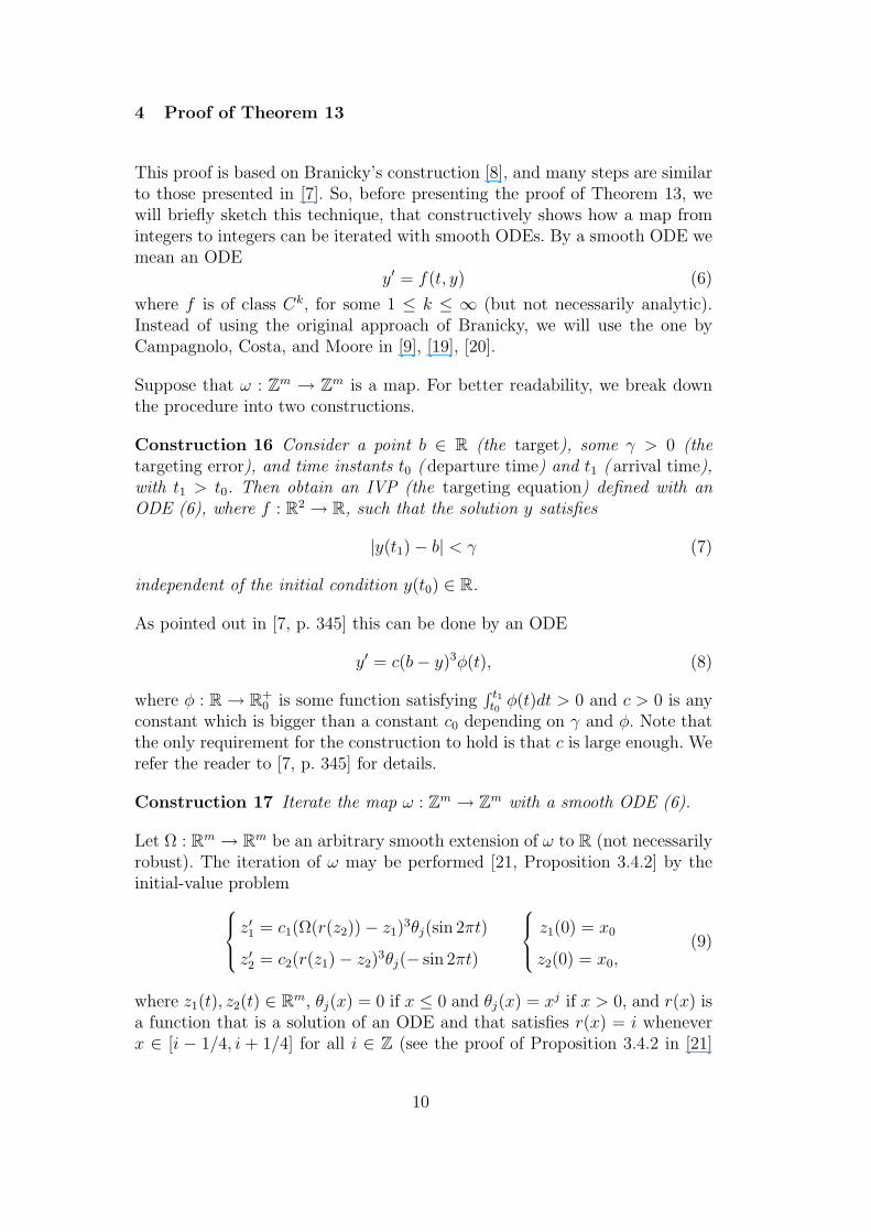
4 Proof of Theorem 13
This proof is based on Branicky’s construction [8], and many steps are similarto those presented in [7]. So, before presenting the proof of Theorem 13, wewill briefly sketch this technique, that constructively shows how a map fromintegers to integers can be iterated with smooth ODEs. By a smooth ODE wemean an ODE
y′ = f(t, y) (6)
where f is of class Ck, for some 1 ≤ k ≤ ∞ (but not necessarily analytic).Instead of using the original approach of Branicky, we will use the one byCampagnolo, Costa, and Moore in [9], [19], [20].
Suppose that ω : Zm → Zm is a map. For better readability, we break downthe procedure into two constructions.
Construction 16 Consider a point b ∈ R (the target), some γ > 0 (thetargeting error), and time instants t0 ( departure time) and t1 ( arrival time),with t1 > t0. Then obtain an IVP (the targeting equation) defined with anODE (6), where f : R2 → R, such that the solution y satisfies
|y(t1)− b| < γ (7)
independent of the initial condition y(t0) ∈ R.
As pointed out in [7, p. 345] this can be done by an ODE
y′ = c(b− y)3φ(t), (8)
where φ : R→ R+0 is some function satisfying
∫ t1t0φ(t)dt > 0 and c > 0 is any
constant which is bigger than a constant c0 depending on γ and φ. Note thatthe only requirement for the construction to hold is that c is large enough. Werefer the reader to [7, p. 345] for details.
Construction 17 Iterate the map ω : Zm → Zm with a smooth ODE (6).
Let Ω : Rm → Rm be an arbitrary smooth extension of ω to R (not necessarilyrobust). The iteration of ω may be performed [21, Proposition 3.4.2] by theinitial-value problem z
′1 = c1(Ω(r(z2))− z1)3θj(sin 2πt)
z′2 = c2(r(z1)− z2)3θj(− sin 2πt)
z1(0) = x0
z2(0) = x0,(9)
where z1(t), z2(t) ∈ Rm, θj(x) = 0 if x ≤ 0 and θj(x) = xj if x > 0, and r(x) isa function that is a solution of an ODE and that satisfies r(x) = i wheneverx ∈ [i − 1/4, i + 1/4] for all i ∈ Z (see the proof of Proposition 3.4.2 in [21]
10
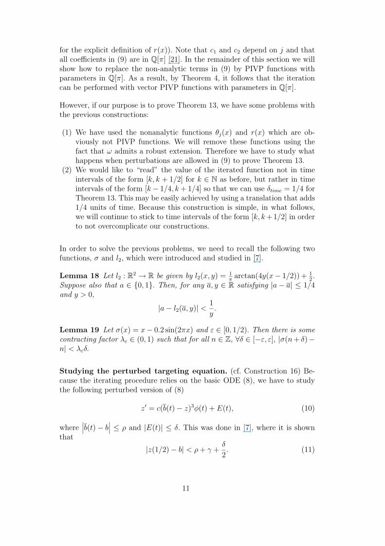
for the explicit definition of r(x)). Note that c1 and c2 depend on j and thatall coefficients in (9) are in Q[π] [21]. In the remainder of this section we willshow how to replace the non-analytic terms in (9) by PIVP functions withparameters in Q[π]. As a result, by Theorem 4, it follows that the iterationcan be performed with vector PIVP functions with parameters in Q[π].
However, if our purpose is to prove Theorem 13, we have some problems withthe previous constructions:
(1) We have used the nonanalytic functions θj(x) and r(x) which are ob-viously not PIVP functions. We will remove these functions using thefact that ω admits a robust extension. Therefore we have to study whathappens when perturbations are allowed in (9) to prove Theorem 13.
(2) We would like to “read” the value of the iterated function not in timeintervals of the form [k, k + 1/2] for k ∈ N as before, but rather in timeintervals of the form [k− 1/4, k+ 1/4] so that we can use δtime = 1/4 forTheorem 13. This may be easily achieved by using a translation that adds1/4 units of time. Because this construction is simple, in what follows,we will continue to stick to time intervals of the form [k, k+ 1/2] in orderto not overcomplicate our constructions.
In order to solve the previous problems, we need to recall the following twofunctions, σ and l2, which were introduced and studied in [7].
Lemma 18 Let l2 : R2 → R be given by l2(x, y) = 1π
arctan(4y(x− 1/2)) + 12.
Suppose also that a ∈ 0, 1. Then, for any a, y ∈ R satisfying |a− a| ≤ 1/4and y > 0,
|a− l2(a, y)| < 1
y.
Lemma 19 Let σ(x) = x− 0.2 sin(2πx) and ε ∈ [0, 1/2). Then there is somecontracting factor λε ∈ (0, 1) such that for all n ∈ Z, ∀δ ∈ [−ε, ε], |σ(n+ δ)−n| < λεδ.
Studying the perturbed targeting equation. (cf. Construction 16) Be-cause the iterating procedure relies on the basic ODE (8), we have to studythe following perturbed version of (8)
z′ = c(b(t)− z)3φ(t) + E(t), (10)
where∣∣∣b(t)− b∣∣∣ ≤ ρ and |E(t)| ≤ δ. This was done in [7], where it is shown
that
|z(1/2)− b| < ρ+ γ +δ
2. (11)
11
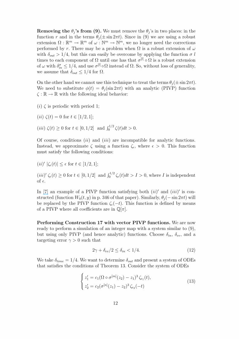
Removing the θj’s from (9). We must remove the θj’s in two places: in thefunction r and in the terms θj(± sin 2πt). Since in (9) we are using a robustextension Ω : Rm → Rm of ω : Nm → Nm, we no longer need the correctionsperformed by r. There may be a problem when Ω is a robust extension of ωwith δout > 1/4, but this can easily be overcome by applying the function σ ltimes to each component of Ω until one has that σ[l] Ω is a robust extensionof ω with δσin ≤ 1/4, and use σ[l]Ω instead of Ω. So, without loss of generality,we assume that δout ≤ 1/4 for Ω.
On the other hand we cannot use this technique to treat the terms θj(± sin 2πt).We need to substitute φ(t) = θj(sin 2πt) with an analytic (PIVP) functionζ : R→ R with the following ideal behavior:
(i) ζ is periodic with period 1;
(ii) ζ(t) = 0 for t ∈ [1/2, 1];
(iii) ζ(t) ≥ 0 for t ∈ [0, 1/2] and∫ 1/2
0 ζ(t)dt > 0.
Of course, conditions (ii) and (iii) are incompatible for analytic functions.Instead, we approximate ζ using a function ζε, where ε > 0. This functionmust satisfy the following conditions:
(ii)′ |ζε(t)| ≤ ε for t ∈ [1/2, 1];
(iii)′ ζε(t) ≥ 0 for t ∈ [0, 1/2] and∫ 1/20 ζε(t)dt > I > 0, where I is independent
of ε.
In [7] an example of a PIVP function satisfying both (ii)′ and (iii)′ is con-structed (function W0(t, y) in p. 346 of that paper). Similarly, θj(− sin 2πt) willbe replaced by the PIVP function ζε(−t). This function is defined by meansof a PIVP where all coefficients are in Q[π].
Performing Construction 17 with vector PIVP functions. We are nowready to perform a simulation of an integer map with a system similar to (9),but using only PIVP (and hence analytic) functions. Choose δin, δev, and atargeting error γ > 0 such that
2γ + δev/2 ≤ δin < 1/4. (12)
We take δtime = 1/4. We want to determine δout and present a system of ODEsthat satisfies the conditions of Theorem 13. Consider the system of ODEs z
′1 = c1(Ω σ[m](z2)− z1)3 ζε1(t),
z′2 = c2(σ[n](z1)− z2)3 ζε2(−t)(13)
12
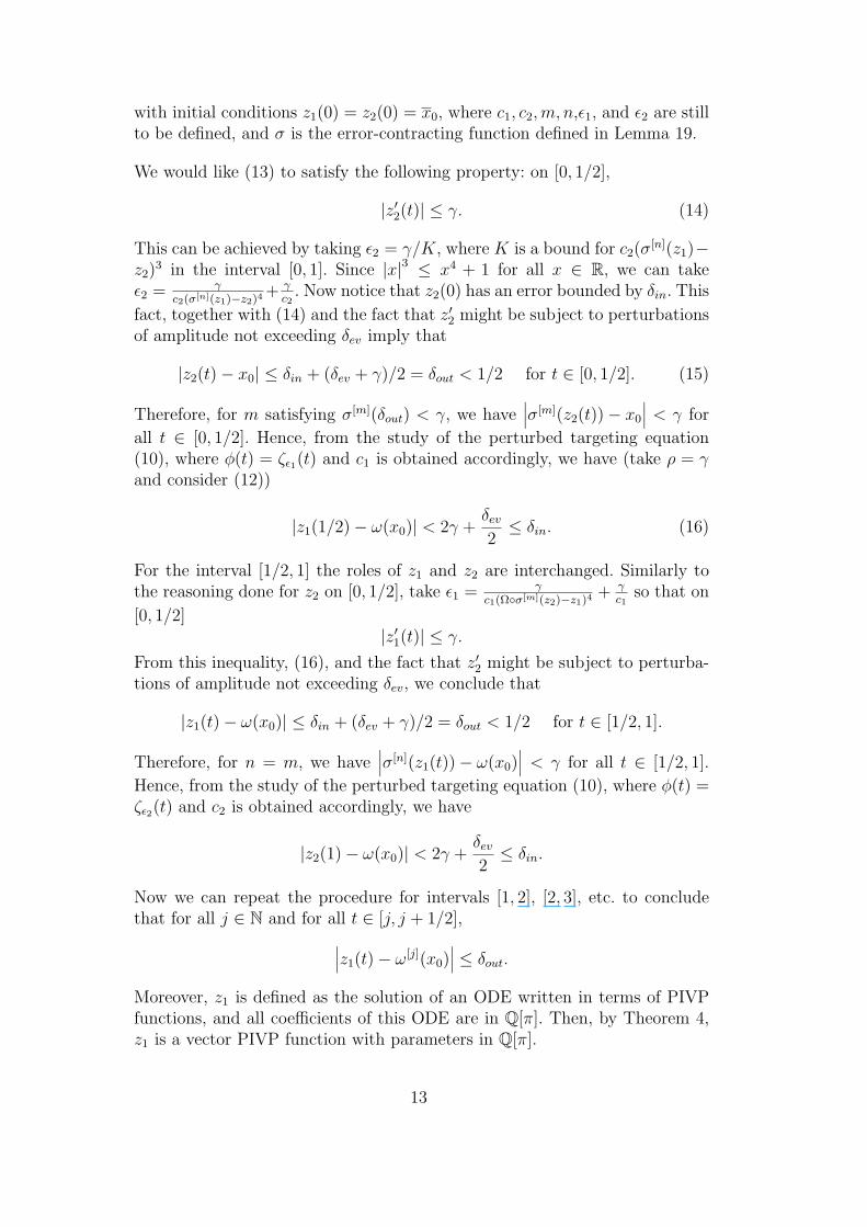
with initial conditions z1(0) = z2(0) = x0, where c1, c2,m, n,ε1, and ε2 are stillto be defined, and σ is the error-contracting function defined in Lemma 19.
We would like (13) to satisfy the following property: on [0, 1/2],
|z′2(t)| ≤ γ. (14)
This can be achieved by taking ε2 = γ/K, where K is a bound for c2(σ[n](z1)−z2)3 in the interval [0, 1]. Since |x|3 ≤ x4 + 1 for all x ∈ R, we can takeε2 = γ
c2(σ[n](z1)−z2)4+ γc2
. Now notice that z2(0) has an error bounded by δin. This
fact, together with (14) and the fact that z′2 might be subject to perturbationsof amplitude not exceeding δev imply that
|z2(t)− x0| ≤ δin + (δev + γ)/2 = δout < 1/2 for t ∈ [0, 1/2]. (15)
Therefore, for m satisfying σ[m](δout) < γ, we have∣∣∣σ[m](z2(t))− x0
∣∣∣ < γ for
all t ∈ [0, 1/2]. Hence, from the study of the perturbed targeting equation(10), where φ(t) = ζε1(t) and c1 is obtained accordingly, we have (take ρ = γand consider (12))
|z1(1/2)− ω(x0)| < 2γ +δev2≤ δin. (16)
For the interval [1/2, 1] the roles of z1 and z2 are interchanged. Similarly tothe reasoning done for z2 on [0, 1/2], take ε1 = γ
c1(Ωσ[m](z2)−z1)4+ γ
c1so that on
[0, 1/2]|z′1(t)| ≤ γ.
From this inequality, (16), and the fact that z′2 might be subject to perturba-tions of amplitude not exceeding δev, we conclude that
|z1(t)− ω(x0)| ≤ δin + (δev + γ)/2 = δout < 1/2 for t ∈ [1/2, 1].
Therefore, for n = m, we have∣∣∣σ[n](z1(t))− ω(x0)
∣∣∣ < γ for all t ∈ [1/2, 1].
Hence, from the study of the perturbed targeting equation (10), where φ(t) =ζε2(t) and c2 is obtained accordingly, we have
|z2(1)− ω(x0)| < 2γ +δev2≤ δin.
Now we can repeat the procedure for intervals [1, 2], [2, 3], etc. to concludethat for all j ∈ N and for all t ∈ [j, j + 1/2],∣∣∣z1(t)− ω[j](x0)
∣∣∣ ≤ δout.
Moreover, z1 is defined as the solution of an ODE written in terms of PIVPfunctions, and all coefficients of this ODE are in Q[π]. Then, by Theorem 4,z1 is a vector PIVP function with parameters in Q[π].
13
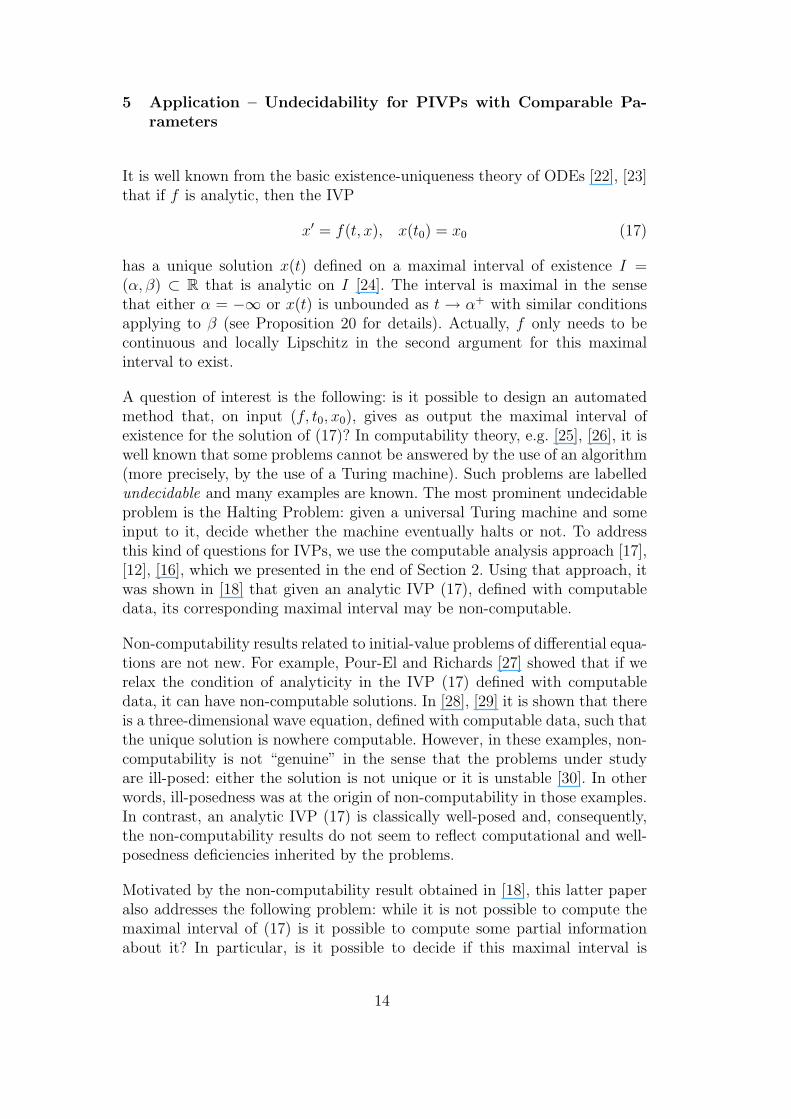
5 Application – Undecidability for PIVPs with Comparable Pa-rameters
It is well known from the basic existence-uniqueness theory of ODEs [22], [23]that if f is analytic, then the IVP
x′ = f(t, x), x(t0) = x0 (17)
has a unique solution x(t) defined on a maximal interval of existence I =(α, β) ⊂ R that is analytic on I [24]. The interval is maximal in the sensethat either α = −∞ or x(t) is unbounded as t → α+ with similar conditionsapplying to β (see Proposition 20 for details). Actually, f only needs to becontinuous and locally Lipschitz in the second argument for this maximalinterval to exist.
A question of interest is the following: is it possible to design an automatedmethod that, on input (f, t0, x0), gives as output the maximal interval ofexistence for the solution of (17)? In computability theory, e.g. [25], [26], it iswell known that some problems cannot be answered by the use of an algorithm(more precisely, by the use of a Turing machine). Such problems are labelledundecidable and many examples are known. The most prominent undecidableproblem is the Halting Problem: given a universal Turing machine and someinput to it, decide whether the machine eventually halts or not. To addressthis kind of questions for IVPs, we use the computable analysis approach [17],[12], [16], which we presented in the end of Section 2. Using that approach, itwas shown in [18] that given an analytic IVP (17), defined with computabledata, its corresponding maximal interval may be non-computable.
Non-computability results related to initial-value problems of differential equa-tions are not new. For example, Pour-El and Richards [27] showed that if werelax the condition of analyticity in the IVP (17) defined with computabledata, it can have non-computable solutions. In [28], [29] it is shown that thereis a three-dimensional wave equation, defined with computable data, such thatthe unique solution is nowhere computable. However, in these examples, non-computability is not “genuine” in the sense that the problems under studyare ill-posed: either the solution is not unique or it is unstable [30]. In otherwords, ill-posedness was at the origin of non-computability in those examples.In contrast, an analytic IVP (17) is classically well-posed and, consequently,the non-computability results do not seem to reflect computational and well-posedness deficiencies inherited by the problems.
Motivated by the non-computability result obtained in [18], this latter paperalso addresses the following problem: while it is not possible to compute themaximal interval of (17) is it possible to compute some partial informationabout it? In particular, is it possible to decide if this maximal interval is
14
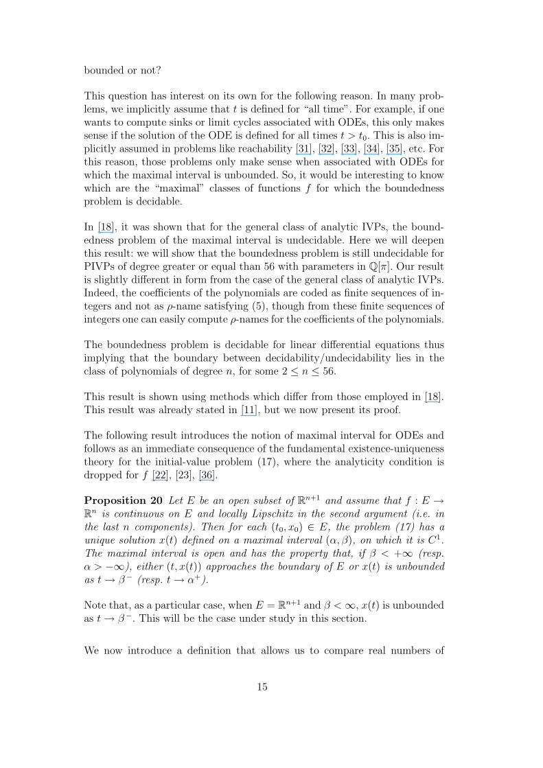
bounded or not?
This question has interest on its own for the following reason. In many prob-lems, we implicitly assume that t is defined for “all time”. For example, if onewants to compute sinks or limit cycles associated with ODEs, this only makessense if the solution of the ODE is defined for all times t > t0. This is also im-plicitly assumed in problems like reachability [31], [32], [33], [34], [35], etc. Forthis reason, those problems only make sense when associated with ODEs forwhich the maximal interval is unbounded. So, it would be interesting to knowwhich are the “maximal” classes of functions f for which the boundednessproblem is decidable.
In [18], it was shown that for the general class of analytic IVPs, the bound-edness problem of the maximal interval is undecidable. Here we will deepenthis result: we will show that the boundedness problem is still undecidable forPIVPs of degree greater or equal than 56 with parameters in Q[π]. Our resultis slightly different in form from the case of the general class of analytic IVPs.Indeed, the coefficients of the polynomials are coded as finite sequences of in-tegers and not as ρ-name satisfying (5), though from these finite sequences ofintegers one can easily compute ρ-names for the coefficients of the polynomials.
The boundedness problem is decidable for linear differential equations thusimplying that the boundary between decidability/undecidability lies in theclass of polynomials of degree n, for some 2 ≤ n ≤ 56.
This result is shown using methods which differ from those employed in [18].This result was already stated in [11], but we now present its proof.
The following result introduces the notion of maximal interval for ODEs andfollows as an immediate consequence of the fundamental existence-uniquenesstheory for the initial-value problem (17), where the analyticity condition isdropped for f [22], [23], [36].
Proposition 20 Let E be an open subset of Rn+1 and assume that f : E →Rn is continuous on E and locally Lipschitz in the second argument (i.e. inthe last n components). Then for each (t0, x0) ∈ E, the problem (17) has aunique solution x(t) defined on a maximal interval (α, β), on which it is C1.The maximal interval is open and has the property that, if β < +∞ (resp.α > −∞), either (t, x(t)) approaches the boundary of E or x(t) is unboundedas t→ β − (resp. t→ α+).
Note that, as a particular case, when E = Rn+1 and β <∞, x(t) is unboundedas t→ β −. This will be the case under study in this section.
We now introduce a definition that allows us to compare real numbers of
15
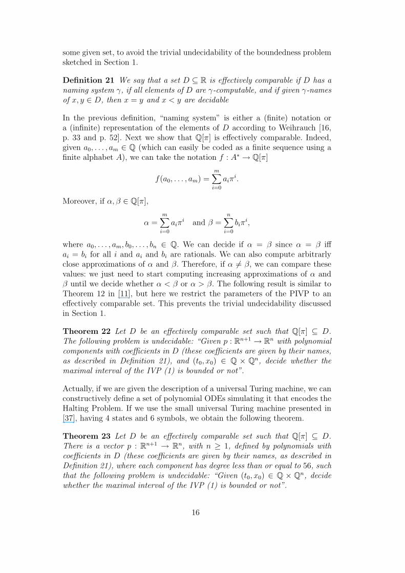
some given set, to avoid the trivial undecidability of the boundedness problemsketched in Section 1.
Definition 21 We say that a set D ⊆ R is effectively comparable if D has anaming system γ, if all elements of D are γ-computable, and if given γ-namesof x, y ∈ D, then x = y and x < y are decidable
In the previous definition, “naming system” is either a (finite) notation ora (infinite) representation of the elements of D according to Weihrauch [16,p. 33 and p. 52]. Next we show that Q[π] is effectively comparable. Indeed,given a0, . . . , am ∈ Q (which can easily be coded as a finite sequence using afinite alphabet A), we can take the notation f : A∗ → Q[π]
f(a0, . . . , am) =m∑i=0
aiπi.
Moreover, if α, β ∈ Q[π],
α =m∑i=0
aiπi and β =
n∑i=0
biπi,
where a0, . . . , am, b0, . . . , bn ∈ Q. We can decide if α = β since α = β iffai = bi for all i and ai and bi are rationals. We can also compute arbitrarlyclose approximations of α and β. Therefore, if α 6= β, we can compare thesevalues: we just need to start computing increasing approximations of α andβ until we decide whether α < β or α > β. The following result is similar toTheorem 12 in [11], but here we restrict the parameters of the PIVP to aneffectively comparable set. This prevents the trivial undecidability discussedin Section 1.
Theorem 22 Let D be an effectively comparable set such that Q[π] ⊆ D.The following problem is undecidable: “Given p : Rn+1 → Rn with polynomialcomponents with coefficients in D (these coefficients are given by their names,as described in Definition 21), and (t0, x0) ∈ Q × Qn, decide whether themaximal interval of the IVP (1) is bounded or not”.
Actually, if we are given the description of a universal Turing machine, we canconstructively define a set of polynomial ODEs simulating it that encodes theHalting Problem. If we use the small universal Turing machine presented in[37], having 4 states and 6 symbols, we obtain the following theorem.
Theorem 23 Let D be an effectively comparable set such that Q[π] ⊆ D.There is a vector p : Rn+1 → Rn, with n ≥ 1, defined by polynomials withcoefficients in D (these coefficients are given by their names, as described inDefinition 21), where each component has degree less than or equal to 56, suchthat the following problem is undecidable: “Given (t0, x0) ∈ Q × Qn, decidewhether the maximal interval of the IVP (1) is bounded or not”.
16
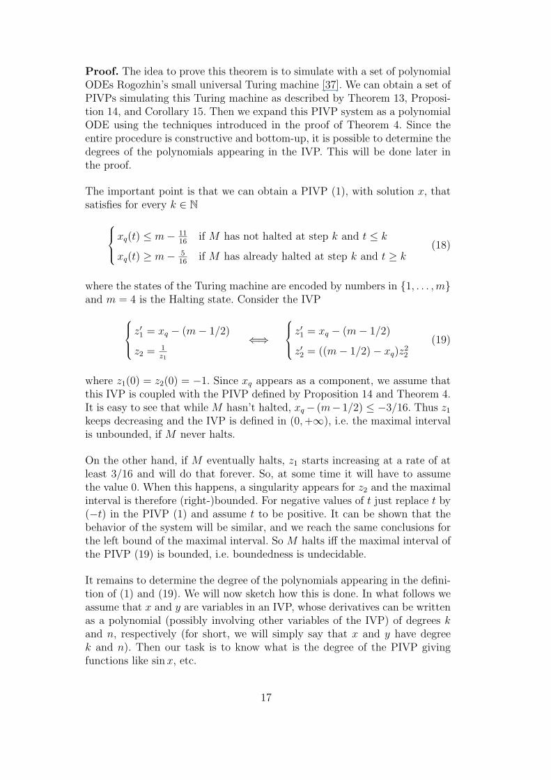
Proof. The idea to prove this theorem is to simulate with a set of polynomialODEs Rogozhin’s small universal Turing machine [37]. We can obtain a set ofPIVPs simulating this Turing machine as described by Theorem 13, Proposi-tion 14, and Corollary 15. Then we expand this PIVP system as a polynomialODE using the techniques introduced in the proof of Theorem 4. Since theentire procedure is constructive and bottom-up, it is possible to determine thedegrees of the polynomials appearing in the IVP. This will be done later inthe proof.
The important point is that we can obtain a PIVP (1), with solution x, thatsatisfies for every k ∈ N
xq(t) ≤ m− 1116
if M has not halted at step k and t ≤ k
xq(t) ≥ m− 516
if M has already halted at step k and t ≥ k(18)
where the states of the Turing machine are encoded by numbers in 1, . . . ,mand m = 4 is the Halting state. Consider the IVP
z′1 = xq − (m− 1/2)
z2 = 1z1
⇐⇒
z′1 = xq − (m− 1/2)
z′2 = ((m− 1/2)− xq)z22
(19)
where z1(0) = z2(0) = −1. Since xq appears as a component, we assume thatthis IVP is coupled with the PIVP defined by Proposition 14 and Theorem 4.It is easy to see that while M hasn’t halted, xq− (m− 1/2) ≤ −3/16. Thus z1
keeps decreasing and the IVP is defined in (0,+∞), i.e. the maximal intervalis unbounded, if M never halts.
On the other hand, if M eventually halts, z1 starts increasing at a rate of atleast 3/16 and will do that forever. So, at some time it will have to assumethe value 0. When this happens, a singularity appears for z2 and the maximalinterval is therefore (right-)bounded. For negative values of t just replace t by(−t) in the PIVP (1) and assume t to be positive. It can be shown that thebehavior of the system will be similar, and we reach the same conclusions forthe left bound of the maximal interval. So M halts iff the maximal interval ofthe PIVP (19) is bounded, i.e. boundedness is undecidable.
It remains to determine the degree of the polynomials appearing in the defini-tion of (1) and (19). We will now sketch how this is done. In what follows weassume that x and y are variables in an IVP, whose derivatives can be writtenas a polynomial (possibly involving other variables of the IVP) of degrees kand n, respectively (for short, we will simply say that x and y have degreek and n). Then our task is to know what is the degree of the PIVP givingfunctions like sin x, etc.
17
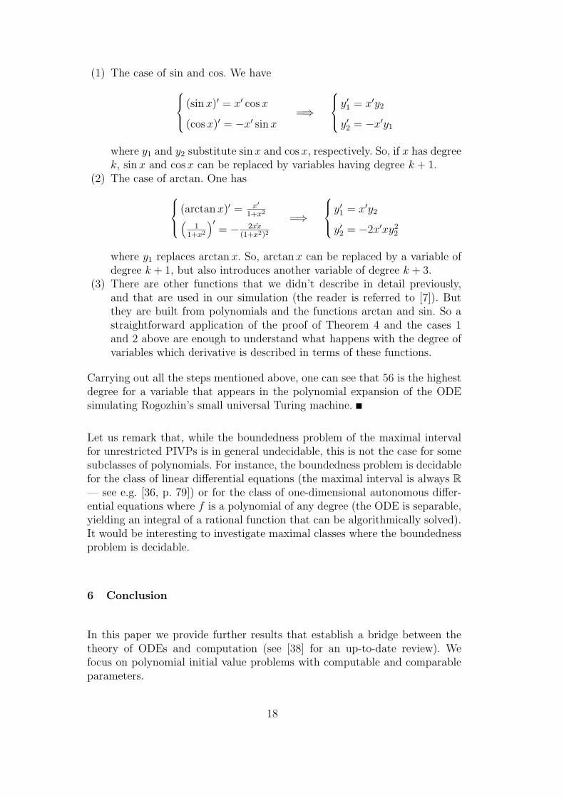
(1) The case of sin and cos. We have (sinx)′ = x′ cosx
(cosx)′ = −x′ sinx=⇒
y′1 = x′y2
y′2 = −x′y1
where y1 and y2 substitute sin x and cos x, respectively. So, if x has degreek, sin x and cos x can be replaced by variables having degree k + 1.
(2) The case of arctan. One has (arctanx)′ = x′
1+x2(1
1+x2
)′= − 2xx
(1+x2)2
=⇒
y′1 = x′y2
y′2 = −2x′xy22
where y1 replaces arctanx. So, arctan x can be replaced by a variable ofdegree k + 1, but also introduces another variable of degree k + 3.
(3) There are other functions that we didn’t describe in detail previously,and that are used in our simulation (the reader is referred to [7]). Butthey are built from polynomials and the functions arctan and sin. So astraightforward application of the proof of Theorem 4 and the cases 1and 2 above are enough to understand what happens with the degree ofvariables which derivative is described in terms of these functions.
Carrying out all the steps mentioned above, one can see that 56 is the highestdegree for a variable that appears in the polynomial expansion of the ODEsimulating Rogozhin’s small universal Turing machine.
Let us remark that, while the boundedness problem of the maximal intervalfor unrestricted PIVPs is in general undecidable, this is not the case for somesubclasses of polynomials. For instance, the boundedness problem is decidablefor the class of linear differential equations (the maximal interval is always R— see e.g. [36, p. 79]) or for the class of one-dimensional autonomous differ-ential equations where f is a polynomial of any degree (the ODE is separable,yielding an integral of a rational function that can be algorithmically solved).It would be interesting to investigate maximal classes where the boundednessproblem is decidable.
6 Conclusion
In this paper we provide further results that establish a bridge between thetheory of ODEs and computation (see [38] for an up-to-date review). Wefocus on polynomial initial value problems with computable and comparableparameters.
18
With respect to computation, our main result is that the boundness of themaximal interval of definition is undecidable even for PIVPs with comparableparameters and degree up to 56. We can view this result as a ODE analog tothe undecidability of the Halting problem for Turing machines.
With respect to polynomial ODEs, we show that they can simulate a largeclass of dynamical systems – including Turing machines – in the presence ofnoise.
Based on the previous results we argue that polynomial ODEs, which are awell known model of physical phenomena, are also a powerful, yet realistic,model of continuous time computation.
Acknowledgments. The authors wish to thank Pieter Collins, Kerry Ojakian,and Ning Zhong, and the anonymous referees for useful remarks and com-ments. DG and MC were partially supported by Fundacao para a Ciencia e aTecnologia and EU FEDER POCTI/POCI via CLC, SQIG - Instituto de Tele-comunicacoes and grant SFRH/BPD/39779/2007 (DG). Additional supportto DG was also provided by the Fundacao Calouste Gulbenkian through thePrograma Gulbenkian de Estımulo a Investigacao. JB was partially supportedby CMAF through FEDER and FCT-Plurianual 2007.
References
[1] M. W. Hirsch, S. Smale, Differential Equations, Dynamical Systems, and LinearAlgebra, Academic Press, 1974.
[2] J. F. Ritt, Integration in Finite Terms. Liouville’s Theory of ElementaryMethods., Columbia Univ. Press, 1948.
[3] C. E. Shannon, Mathematical theory of the differential analyzer, J. Math. Phys.MIT 20 (1941) 337–354.
[4] D. S. Graca, J. F. Costa, Analog computers and recursive functions over thereals, J. Complexity 19 (5) (2003) 644–664.
[5] J. H. Hubbard, B. H. West, Differential Equations: A Dynamical SystemsApproach — Higher-Dimensional Systems, Springer, 1995.
[6] D. S. Graca, N. Zhong, J. Buescu, The ordinary differential equation defined bya computable function whose maximal interval of existence is non-computable,in: G. Hanrot, P. Zimmermann (Eds.), Proceedings of the 7th Conference onReal Numbers and Computers (RNC 7), LORIA/INRIA, 2006, pp. 33–40.
[7] D. S. Graca, M. L. Campagnolo, J. Buescu, Computability with polynomialdifferential equations, Adv. Appl. Math. 40 (3) (2008) 330–349.
19
[8] M. S. Branicky, Universal computation and other capabilities of hybrid andcontinuous dynamical systems, Theoret. Comput. Sci. 138 (1) (1995) 67–100.
[9] M. L. Campagnolo, C. Moore, J. F. Costa, Iteration, inequalities, anddifferentiability in analog computers, J. Complexity 16 (4) (2000) 642–660.
[10] E. Hainry, Reachability in linear dynamical systems, in: A. Beckmann,C. Dimitracopoulos, B. Lowe (Eds.), Computability in Europe 2008 (CiE 2008),Vol. 5028 of LNCS, 2008.
[11] D. S. Graca, J. Buescu, M. L. Campagnolo, Boundedness of the domain ofdefinition is undecidable for polynomial ODEs, in: R. Dillhage, T. Grubba,A. Sorbi, K. Weihrauch, N. Zhong (Eds.), Proceedings of the 4th InternationalConference on Computability and Complexity in Analysis (CCA 2007),FernUniversitat in Hagen, 2007, pp. 127–135.
[12] K.-I. Ko, Computational Complexity of Real Functions, Birkhauser, 1991.
[13] L. A. Rubel, F. Singer, A differentially algebraic elimination theorem withapplication to analog computability in the calculus of variations, Proc. Amer.Math. Soc. 94 (4) (1985) 653–658.
[14] D. S. Graca, Some recent developments on Shannon’s General Purpose AnalogComputer, Math. Log. Quart. 50 (4-5) (2004) 473–485.
[15] M. B. Pour-El, Abstract computability and its relations to the general purposeanalog computer, Trans. Amer. Math. Soc. 199 (1974) 1–28.
[16] K. Weihrauch, Computable Analysis: an Introduction, Springer, 2000.
[17] M. B. Pour-El, J. I. Richards, Computability in Analysis and Physics, Springer,1989.
[18] D. Graca, N. Zhong, J. Buescu, Computability, noncomputability andundecidability of maximal intervals of IVPs, Trans. Amer. Math. Soc.To appear.
[19] M. Campagnolo, C. Moore, Upper and lower bounds on continuous-timecomputation, in: I. Antoniou, C. Calude, M. Dinneen (Eds.), 2nd InternationalConference on Unconventional Models of Computation - UMC’2K, Springer,2001, pp. 135–153.
[20] M. L. Campagnolo, Computational complexity of real valued recursive functionsand analog circuits, Ph.D. thesis, Instituto Superior Tecnico/UniversidadeTecnica de Lisboa (2002).
[21] M. L. Campagnolo, The complexity of real recursive functions, in: C. S.Calude, M. J. Dinneen, F. Peper (Eds.), Unconventional Models of Computation(UMC’02), LNCS 2509, Springer, 2002, pp. 1–14.
[22] E. A. Coddington, N. Levinson, Theory of Ordinary Differential Equations,McGraw-Hill, 1955.
[23] S. Lefshetz, Differential Equations: Geometric Theory, 2nd Edition,Interscience, 1965.
20
[24] V. I. Arnold, Ordinary Differential Equations, MIT Press, 1978.
[25] M. Sipser, Introduction to the Theory of Computation, PWS PublishingCompany, 1997.
[26] J. E. Hopcroft, R. Motwani, J. D. Ullman, Introduction to Automata Theory,Languages, and Computation, 2nd Edition, Addison-Wesley, 2001.
[27] M. B. Pour-El, J. I. Richards, A computable ordinary differential equation whichpossesses no computable solution, Ann. Math. Logic 17 (1979) 61–90.
[28] M. B. Pour-El, J. I. Richards, The wave equation with computable initial datasuch that its unique solution is not computable, Adv. Math. 39 (1981) 215–239.
[29] M. B. Pour-El, N. Zhong, The wave equation with computable initial data whoseunique solution is nowhere computable, Math. Log. Quart. 43 (1997) 499–509.
[30] K. Weihrauch, N. Zhong, Is wave propagation computable or can wavecomputers beat the Turing machine?, Proc. London Math. Soc. 85 (3) (2002)312–332.
[31] R. Alur, D. L. Dill, Automata for modeling real-time systems, in: Automata,Languages and Programming, 17th International Colloquium, LNCS 443,Springer, 1990, pp. 322–335.
[32] E. Asarin, O. Maler, A. Pnueli, Reachability analysis of dynamical systemshaving piecewise-constant derivatives, Theoret. Comput. Sci. 138 (1995) 35–65.
[33] T. A. Henzinger, P. W. Kopke, A. Puri, P. Varaiya, What’s decidable abouthybrid automata?, J. Comput. System Sci. 57 (1) (1998) 94–124.
[34] O. Bournez, Achilles and the Tortoise climbing up the hyper-arithmeticalhierarchy, Theoret. Comput. Sci. 210 (1) (1999) 21–71.
[35] V. D. Blondel, J. N. Tsitsiklis, A survey of computational complexity results insystems and control, Automatica 9 (36) (2000) 1249–1274.
[36] J. K. Hale, Ordinary Differential Equations, 2nd Edition, Robert E. KriegerPub. Co, 1980.
[37] Y. Rogozhin, Small universal Turing machines, Theoret. Comput. Sci. 168 (2)(1996) 215–240.
[38] O. Bournez, M. L. Campagnolo, New Computational Paradigms. ChangingConceptions of What is Computable, Springer-Verlag, New York, 2008, Ch.A Survey on Continuous Time Computations, pp. 383–423.
21


