POLYNOMIAL ROOTS AND OPEN MAPPINGS

Jon A. Sjogren

Faculty of Graduate Studies, Towson University

1 June 2015

Plan of Argument

We examine a class of proofs to the Fundamental Theorem of Algebra thatrelate to partial open mappings of the complex plane. These proofs use the “open”property of a complex polynomial, at points of its domain. Based on proofs byF.S. Cater and D. Reem, we know using only elementary analysis that a non-constant polynomial is in fact open. This fact, which is easily derived using thenon-elementary tools of complex analysis, may be more technical than necessaryfor proving FTA. In any case, combined with the Principle of S. Reich that for apolynomial P (z), the image set P (C) is also closed (the mapping P (z) is proper),the proof is already finished!

Another approach is to exploit the openness that holds away from critical pointsand critical values. What is needed follows from the Inverse and Implicit FunctionTheorems. One of the simplest and best of all proofs of FTA is due to [Wolfenstein],who shows that critical points and values are easily dealt with. A related proof givenbelow is reminiscent of the Argaud-Cauchy-Littlewood method, where one showsthat if P (z0) 6= 0, some z1 ∈ C can always be found so that |P (z1)| < |P (z0)|. Itturns out that this proof was already sketched out in Smale’s survey article [Smale],where the author tacitly makes use of Reich’s Principle, so it could be called theReich-Smale Proof.

The proof of FTA from J. Milnor’s published notes “Topology from the Differ-entiable Viewpoint”, [TFDV], is examined next as it also deals with topologicalproperties of the given polynomial mapping P (z). The fact that P (z) is proper(has the “propriety” property) is used to compactify the mapping, making it pos-sible to use a “Pre-Image” result from differential topology to establish that themapping, in the non-constant case, is surjective. This argument, which uses the“locally constant” nature of a counting function for the pre-image points of thecompactified polynomial, goes forward because of propriety. In fact it is Reich’sPrinciple that allows P to be extended to a compact manifold (the two-sphere S2).

The final word on giving a modern cast to Gauss’s first proof (Thesis 1799)appears in [Gersten-Stallings]. The blend of differential topology with the geomet-ric theory of free groups may have resulted in the paper not being much quoted,except by Martin, Savitt and Singer, referred to as [MSS], who study the combi-natorics of harmonic functions and their graphs. These authors come up with anew proof of FTA along the lines of Gauss I. This proof has elegant features but

Typeset by AMS-TEX

1

2 JON A. SJOGREN

does not dwell on the rigor of the topological argument. It takes as second natureseveral observations on plane curves from the algebraic side that were overlookedin [Gersten-Stallings].

It should be enough for grounding in the Gauss I proof, to read [Ostrowski],[Gersten-Stallings], [MSS] and the present report. From the Ostrowski paper, onlythe first sections on “the exterior of the large circle” are used here, or much quotedby [Smale] or by others. A scholar with fortitude can attempt the Master’s original[Gauss]. In addition, references such as the text [Guillemin & Pollack], a sourceof multivariate methods such as [C.H. Edwards], and a primer on plane curves [G.Fischer] will be helpful.

As pointed out by S. Smale in his survey, the assumptions without proof madeby Gauss about algebraic curves were not dealt with until the 1920’s, long after thedevelopment of much of “higher” algebraic geometry. Our current understandingof point sets, contraction mappings etc., no doubt makes the task so brilliantlyattacked by Gauss more tractable. We hope that further improvement along indi-cated lines will be forthcoming. The author thanks Prof. Chao Lu and colleagues atTowson University for sharing related algorithmic work. The author also is gratefulto Dr. Daniel Reem of IMPA for his keen interest in the topic, and for suggestinga number of specific improvements to the presentation.

The Principle of S. Reich

A straightforward way to prove the Fundamental Theorem of Algebra is to ob-serve that if P (z) is a polynomial of degree ≥ 1, the image set P (C) is both openand closed in Cw (the “target plane”). Since the latter “space” is also connected,we have P (Cz) = Cw, where Cz is the “source” complex plane, and certainlyOw = 0 + i0 ∈ Cw belongs to the image.

In fact any complex polynomial gives a closed mapping [S. Reich]. In the case ofa constant P (deg P = 0), this result is clear. For deg P (z) = n ≥ 1 we know that[Hille] for some R > 0, any z with |z| ≥ R yields |P (z)| ≥ 1

2 |z|n, hence {|zi|} → ∞implies {|P (zj)|} → ∞. This means by definition that P : Cz → Cw is proper (theinverse image of a compact set K ⊂ Cw is always compact).

We now state a usable form of the Inverse Function Theorem. An “analytic”function defined on an open set U is one that has a convergent power series on U .

Proposition. Suppose f : U ⊂ Cz → Cw is analytic on U with f ′(p) 6= 0,p ∈ U . Then there is an open neighborhood V of v = f(p) and an analytic functiong = V → U such that z ∈ g(V ) implies that z = g ◦ f(z) and w ∈ V impliesw = f ◦ g(w). �

Thus at a regular point of f , where the derivative does not vanish, an analyticinverse can be found on some neighborhood of the image value. The inverse functiong maps V injectively onto an open set of Cz. We will subsequently derive thisProposition from the Implicit Function Theorem.

One of the differences between R and C is that while polynomials defined oneither field are continuous, proper, and closed, a polynomial with an extremum atx0 ∈ R is not open on a small neighborhood of x0.

3

The use of contour integrals allows for a beautiful explicit formula for the inversesuch as

g(v) =1

2πi

∮

γ

tf ′(t)

f(t)− vdt

for a simple contour γ contained in U that holds v in its interior. In any case wehave f(p) contained in a Cw-neighborhood V of image values meaning that f isopen away from the set B ⊂ Cz of singular points, where the derivative vanishes.We are ready for

Fundamental Theorem of Algebra. ([Wolfenstein, 1967]).Proof. Let P (z) have degree n ≥ 0. Let S = P (Cz) which is closed in Cw by

Reich’s Principle so Cw−S is open. As long as P is not constant, B := {z : P ′(z) =0} is finite in Cz since P

′(z) has degree n−1. Hence T = P (B) is finite and Cw−Tis connected. (There is a polygonal arc connecting w1, w2 ∈ Cw − T within thatspace, see [Dugundji, V.2.2])

Every w0 ∈ S−T satisfies w0 = P (z0) for some z0 ∈ Cz −B, hence is a “regularvalue” for P . The Inverse Function Theorem now asserts that some neighborhood ofw0 maps analytically by a function locally the inverse of P (z) onto a neighborhoodof z0. Therefore, S − T is open in Cw. Writing

Cw − T = (Cw − S) ∪ (S − T ),

we are faced with a disjoint union of open sets. The left-hand side is connected,so if the image S does not fill up Cw, we must have S − T = ∅. But S is thecontinuous image of connected Cz, so is connected, and T is discrete, so S itselfmust be a one-point set {w0}. Hence P (z) must be a constant function (of degree0), otherwise P (z) is surjective and certainly has a root. �

Before we move on to methods needing deeper concepts from topology and poly-nomial algebra, we consider a new proof combining elements of the Wolfensteinproof with another one found in [Thompson]. The visualization of this new proof,which could be called the Reich-Smale approach, may appeal to some researchers.

Proof of Reich-Smale FTA. Consider a bounded neighborhood E in a 45◦

sector of Cz. As z ranges over E, the image values {P (z)} can be made to rangewithin a 45◦ sector of Cw by shrinking E. We assume that 0 ∈ Cw is not inthe image. Also we are assured that not all of E maps to a particular radial line(ray to the origin). For one may pick a point z0 ∈ E where P ′(z0) 6= 0, else thederivative would vanish on an open set and the polynomial would be degenerate(constant). Furthermore let E0 ⊂ E be open and contain z0. Then the InverseFunction Theorem implies that some open set of Cw containing w0 = P (z0) is theanalytic image under P of a subset of E0. In particular, P is continuous, injectiveand surjective from the subset of E0 to its image. Thus a line segment such as partof a radial ray cannot contain the image of E0. Note how it is important to keep theimage from submerging onto a radial, whereas in the Cater proof to follow, aboutthe openness of a polynomial function, one places image points onto a radial ray.

Now we take z1, z2 close enough in E, and connect them with a line segmentl ⊂ Cz, with P (l) not on any radial, hence w1 = P (z1), w2 = P (z2) have diversearguments (complex phases differ). By compactness, the set P (l) realizes its maxi-mum modulus at a value w∗ = P (z∗). Now by the propriety of P , we can choose R

4 JON A. SJOGREN

large enough so that |z| > R implies that |P (z)| > |w∗|, and let AR := {z : |z| ≤ R}.Then we know that between θ1 = argw1 and θ2 = argw2, every θ with θ1 ≤ θ ≤ θ2leads to ρeiθ = P (z) for some z ∈ AR. We make take without loss of generality theangles 0 ≤ θ1 < θ2 < 2π as lying within some 45◦ circular sector. A real quantitydepending on θ is

ρθ = inf{

ρ : w = ρeiθ = P (z) for some z ∈ AR}

.

The modulus ρθ is attained by P (z) on AR so we can define

wθ = ρθeiθ.

For the continuum of allowed values of the parameter θ, not all wθ can be critical

values of P ! Thus we pick θ ∈ [θ1, θ2] where wθ is a regular value. See [Figure A].

z

AR

Sector

E

R

lz1

z2

O

w

O

θθ′

wθ′wθ

w2

θ

w∗

P (l)

w1

Figure A

5

On the one hand, by minimality, there is no 0 < ρ < ρθ such that there exists

z′ ∈ AR with P (z′) = ρeiθ. On the other hand, wθ as a regular image point underP , is interior to an open set of other regular values, each having a pre-image. Thus

there is a value P (z′′), z′′ ∈ AR having the argument θ, which is closer to the originOw than is P (z).

The point z′′ must lie in AR, since the complement of AR in Cz, call it BR, mapsentirely to values w = P (z) satisfying

|w| > |w∗| ≥ |P (z)| > |P (z′′)| .

The construction of z′′ gives a contradiction which shows that P : Cz → Cw musthave a root, and in fact is surjective. �

The present “original” proof of FTA just given can be seen as simplifying the[Thompson] and the Milnor [TFDV] proofs, and is somewhat less abstract than theWolfenstein proof. It retains the essence of the classic Argaud-Cauchy-Littlewoodmethod, (see [Littlewood]), but is is really the same as a proof sketched out in the“computational” survey of [Smale]. The author Prof. Smale uses “propriety” orthe “closed property” implicitly, and did not banner the result as a theorem, so wepropose to call what we just detailed, the “Reich-Smale proof” of FTA.

Again, the main point is the predominance of regular points and regular values.Although an arbitrary complex polynomial turns out to be an open mapping Cz →Cw, this is a more obvious (local) fact when the complex derivative is non-zero. Inthat case the Inverse Function Theorem shows that a “compact” image set avoidingthe origin must actually be “open” and hence include it. This contradiction showsthat AR must contain a root of P , or else be constant.

Remarks on Milnor’s Proof

In his “iconic” set of lecture notes of 1965, “Topology from the DifferentiableViewpoint” [TFDV], J. Milnor gave a new proof of FTA that received wide atten-tion. The Fundamental Theorem of Algebra was displayed as an exercise in thecategory of smooth compact manifolds and their mappings. Milnor resorts to theartifice of compactifying complex planes Cz and Cw, which necessitates conjugationby stereographic projections etc. But working with compact spaces is consistentwith the theme of the book [TFDV].

Consider the smooth mapping f : S2 → S2, derived from the original polynomialP : Cz → Cw. One observes that the sets of critical points {κ} ⊂ Cz and criti-cal values {τ} ⊂ Cw are discrete and finite, so their complements are connected,similar to as comes up in Wolfenstein’s proof. An interesting aspect of the proofis the author’s verification that f is smooth at the North Pole of Cz, where in factf(Northz) = Northw. This amounts to nothing less than the Reich Principle (f isa closed mapping), so essential to an FTA proof of the type we are considering.

We quote freely from [TFDV]. Given f :M → N smooth,

“for ... a regular value y, we define #f−1(y) to be the number of points inf−1(y).”

“The first observation to be made about #f−1(y) is that it is locally constantas a function of y (running through regular values!). I.e., there is a neighborhoodV ⊂ N such that y′ ∈ V implies #f−1(y′) = #f−1(y).”

6 JON A. SJOGREN

A brief demonstration of this last quotation starts with “let x1, . . . , xk be thepoints of f−1(y), and choose pairwise disjoint neighborhoods U1, . . . , Uk of these...”From this results the invariance of the integer k as y varies over an open set. In thecase f−1(y) = ∅, the omitted proof would be that since M was assumed compact,f must be proper, so its image is closed in N . Hence the set of “non-image” regularvalues {y} is also open.

A function such as F (x, y) = (ex cos y, ex sin y) cannot be extended continuouslyto the Riemann sphere S

2. Indeed (0, 0) ∈ R2w is an isolated regular value with no

pre-image, but every other value in Cw does have some pre-image. The derivativematrix always has full rank, since the derivative ez never vanishes. The fact thatnon-image values form an open set is critical to Milnor’s proof of FTA. A functionsuch as ez is not a proper mapping from Cz → Cw. On the other hand, the set{w : ∀z, P (z) 6= w} is the complement of the image set S = P (Cz) hence is open,since P is continuous and proper, hence closed. Thus for a polynomial P (z), andf derived from it, #P−1(w) and #f−1(w) can be defined and is locally constant.

Although there are by now a number of proofs of FTA referring to open map-pings and critical points, Milnor’s book shows the relevance of modern differentialtopology. The Pre-Image Theorem is central to the treatment of the Gauss Proof(Thesis, Univ. Helmstedt 1799) as in [Gersten-Stallings]; instead we emphasize therelated but more basic Implicit Function Theorem.

The Complex Polynomial as an Open Mapping

We review the argument that a non-constant complex polynomial maps everyopen planar set onto another open set. The simplifications from modern proofs thatcover any analytic function are not substantial —one can apply them to the case ofa “finite power series” or polynomial. The desired result, which immediately yieldsthat P (Cz) is open, leads to the Fundamental Theorem of Algebra that P (Cz) = Cw

for deg P (z) ≥ 1, since this space is also closed by Reich’s Principle, and Cw isconnected.

Theorem (Complex Polynomials). If f(z) = zk + an−1zk−1 + · · · + ajz

j,n ≥ 1, j ≥ 0, ak ∈ C for k = j, j + 1, . . . , k − 1, and aj 6= 0.

Then there exists δ > 0 real such that |w| < δ implies that w ∈ f(Cz); hencef is open at Oz. Thus our situation is that the polynomial f is of degree n (wemay write ak = 1 if called for), is not constant on any neighborhood, and satisfiesf(0) = 0. By translating f(z) we see at once that f(Cz) ⊂ Cw is also an open set.

Proof of Theorem. Take r > 0 so small that

(1) rn +n−1∑

i=j+1

|ai|ri < |aj |rj (aj 6= 0).

The inequality (1) will also hold for smaller r′, 0 < r′ < r. Next, consider theclosed r-disc D ⊂ Cz, D = {z : |z| ≤ r} with B = ∂D, the complex numbers ofmodulus r. Since f is continuous, f(B) is compact and inf |f(b)| is realized at someb0 ∈ B and we let d = |f(b0)| with δ = d/2.

Given t ∈ Cw satisfying |t| < δ = d/2, it is sufficient for the conclusion of theTheorem to show that t ∈ f(D). Let us assume otherwise, by compactness we can

7

realize inf{|t − f(z)| : z ∈ D} by the choice of some v ∈ D, letting q = t − f(z),noting that |q| > 0. But v is not in B, since the value t is closer to f(Oz) = Owthan to f(B), given inf{|t − f(b)| : b ∈ B} ≥ d/2, since t was chosen closer in toOw than half the radius d = inf{|w| : w ∈ f(B)}. See [Figure B].

tδ

Ow

f(b0)

f(B)

Figure B

In any case f(b) never takes the value Ow when r is chosen small as above. Forthat would entail, for |z| = r, that

∣

∣ajzj∣

∣ = |aj |rj =

∣

∣

∣

∣

∣

∣

znn−1∑

i=j+1

aizi

∣

∣

∣

∣

∣

∣

≤ rn +n−1∑

i=j+1

|ai|ri

which violates our postulated inequality (1).We recapitulate the situation regarding points and values. The value t ∈ Cw was

chosen closer to f(Oz) = Ow than to any f(b), b ∈ B. We find v ∈ D that makes|t−f(v)| minimal. Hence v cannot belong to B = ∂D since Oz ∈ D and |t−f(Oz)|would be smaller than this minimum. In short, v ∈ D\B so |v| < r.

We are now in a position to recalibrate the function f with v as the new base pointof a Taylor series. In other words we obtain f(v+ h) = hn + bn−1h

n−1 + · · ·+ bshs

where s ≥ 0, bn ≥ 1 and bs 6= 0. We note that the degree of f in the new variabledid not change.

8 JON A. SJOGREN

Since |v| < r, we may choose β ∈ R so that all the following hold:

i) 0 < β < r − |v|

ii)

n∑

k=s+1

|bn|βk−s < |bs|, and since q = t− f(z) 6= 0.

iii) |bs|βs < |q|

Now express in polar form:

bs = |bs|eiθ 0 ≤ θ < 2π

q = |q|eiϕ 0 ≤ ϕ < 2π

and choose 0 ≤ ϕ < 2π such that

s · ψ + θ = ϕ mod (2π) .

t− f(v)

bsps

bs

Ow

p = βeiψ

Figure C

Take p = βeiψ, so that bsps and q = t−f(v) have the same argument mod (2π).

See [Figure C]. Using iii) above, |bsps| < |q|. Therefore since these values lie on acommon radial,

|q| − |bsps| = |t− f(v)− bsps|

and from ii),

∣

∣

∣

∣

∣

n∑

k=s+1

bkpk

∣

∣

∣

∣

∣

< |bsps| ,

9

so we finally obtain

|t− f(v + p)| =∣

∣

∣

∣

∣

t− f(v)− bsps −

n∑

k=s+1

bkpk

∣

∣

∣

∣

∣

≤ |t− f(v)− bsps|+

∣

∣

∣

∣

∣

n∑

k=s+1

bkpk

∣

∣

∣

∣

∣

=

= |t− f(v)| − |bsps|+∣

∣

∣

∣

∣

n∑

k=s+1

bkpk

∣

∣

∣

∣

∣

< |t− f(v)| .

We must additionally understand why v + p ∈ D holds true. But

|v + p| ≤ |v|+ |p| = |v|+ β < r

by i). Thus v+p ∈ D, but |t−f(v+p)| being strictly smaller than |t−f(v)|, definedas the infimum of all |t− f(z)|, z ∈ D, gives a contradiction. Hence t ∈ f(D) afterall and Ow = f(Oz) is contained in a neighborhood U(Ow) entirely in the imagef(D) ⊂ f(Cz). Translating the polynomial in the image plane as necessary werecover

Theorem. When f : Cz → Cw is a polynomial function of degree n ≥ 1, if U isopen in Cz then f(U) is open in Cw. In particular f(Cz) is always an open set inthe complex metric topology. �

Intersection Geometry of Plane Curves

For a real (plane) algebraic “curve” defined by F (x, y) = 0 where F is a poly-nomial in two variables, it is often desired to exhibit some part of the locus as asmooth curve in the sense of analytic geometry. In particular, Gauss’s First Proof[Gauss, 1799] exhibits solutions to f(z) = 0 as the common points of two smoothcurves in a planar domain D ⊂ R

2 (each with several components). Gauss’s spec-ulation on the topological nature of these real curves was evidently premature, thereal numbers not yet having been precisely defined. Criticism has continued untilthe present day with the “completion” work of Ostrowski clarifying some but not allof the obscurities in Gauss’s arguments. In fact Uspensky, who probably knew thework of Ostrowski as well as anyone, gives only a summary of it in his book. Smalein his survey lauds the Ostrowski work on Gauss I without elaboration: instead heoffers his own much simpler proof of FTA, the Reich-Smale argument.

The key to parametrizing an algebraic curve is the Implicit Function Theorem.We have need of this theorem in its classical form, but the proof we present isa modern one that is recommended by authorities on (several) complex variabletheory.

Our intention is to go through an up-to-date version of Gauss I, driven by the pa-per [Gersten-Stallings]. This article is also cited by [MSS] of J. Martin et al., whichgives a similar proof using new features, but taking the topological stipulationsof [Gersten-Stallings] at face value. The paper [MSS] is directed at combinatorialstructures that arise from the interplay of the curves g(x, y) = 0, h(x, y) = 0 whenf(z) = f(x+ iy) = g(x, y) + ih(x, y).

We redo all the geometry of [Gersten-Stallings] for several reasons. Firstly, itis hardly a good sign to construct regular values of a mapping by using Sard’s(non-deterministic) theorem, when the set of critical points (and critical values) is

10 JON A. SJOGREN

finite in the first place. One realizes that features of the problem not of interest tothe authors are ignored, including certain geometric simplifications. An example isthat conceivably g−1(0) ⊂ R2

z could contain some closed 1-manifold components,but this is not the case since g(x, y) is a harmonic function satisfying the Maxi-mum Principle. The “deep point” of the authors’ proof involves the “topology ofa 2-cell” and the Jordan Curve Theorem. We try to make such statements moreprecise without necessitating a foray into geometric group theory that seems orig-inally adapted to surfaces of genus greater than 0. Sweeping statements are maderegarding the convergence of g(reiθ), “uniformly with all its derivatives”, but in-stead of pursuing such results, we find that the first Sections of Ostrowski’s paper,the part quoted in Uspensky’s book, yield sufficient geometric information to dothe job. See [Uspensky].

The present author admits that by now his (condensed) critique of the [Gersten-Stallings] paper has gone on about as long as that paper itself. One major reason toreconsider this worthwhile article is its use of the “extended Pre-Image Theorem”,already referred to, that requires a certain mapping to be regular on two differentspaces (at the same point). It may be advisable to avoid such an arcane result,especially where we have at hand a visual context of two real variables. You shouldbe able to see the roots emerge as intersections before your eyes! Instead of the“pre-image as manifold” result, we use the Implicit Function Theorem as our maintool.

The Latest on Gauss’s Thesis (1799)

We consider Gauss’s First Proof to fall into the category of proofs based on theopen mapping concept. This is because of its critical dependence on the ImplicitFunction Theorem and the construction of a 1-manifold or plane curve componentusing an open cover.

Several writings seemed to represent the “final word” in describing Gauss’s proof,making it sufficiently convincing. This report will not fully achieve such a goaleither. Additionally looking through [Gersten-Stallings 1988], [Ostrowski 1920],and [MSS 2002] should provide a good picture of how to carry through Gauss I withmodern methods. Somewhat more difficult than these papers is the original Thesisof Gauss, “Demonstratio nova Theorematis omnem functionem...”. A synopsis ofessential portions of the Ostrowski article, which brought the Gauss proof back toa good reputation, is given in the books of [Uspensky, Appendix I], or [Fine &Rosenberger].

We are going to follow the [Gersten-Stallings] model, but with refinements basedon elementary observations about real plane curves. A first aspect is the “pre-image” theorem from differential topology, where a given g−1(y) is seen to be a“one-manifold”. The desired properties of this point set are then derived from acharacterization of an “abstract” one-manifold. We work with concrete curves andarcs, to the extent that “one-manifold” becomes superfluous. In particular, we canavoid the full strength of the Pre-Image Theorem. The treatment of this result inwell-known books has been debated: we try to step around issues such as a mappingbeing transverse to a point set, and also to the boundary of this point set. We areable to avoid use of Sard’s theorem with its nondeterministic implications by notingas does Milnor on [TFDV p. 8] that the sets of critical points and critical valuesare both finite.

11

The article [MSS] gives a nice geometric approach different from [Gersten-Sta-llings], by adjusting the component curves instead of the polynomial itself, buttakes the needed topological tools for granted. We do not use the Jordan CurveTheorem at all, falling back on a simpler result that is a prelude to the JCT itself.Also we simplify the final combinatorial step, at the cost of obtaining only one rootof the polynomial, not the full contingent of n roots at one time, which the JordanCurve methods of [MSS] might achieve.

A. Ostrowski’s treatment of a locus of zeros (a real variety) has been much quotedin its aspect “toward infinity”. The critical element was where Gauss admitted thathe had not proved that an algebraic curve that “runs into a limited space must runout again”. Ostrowski’s clarification of this “limited” issue has been completelyaccepted, but not carried through into any textbook, except by a few drawings[Uspensky, Appendix I].

Thus it is well to attack the problem from scratch. We have a monic complexpolynomial

f(z) = zn + bn−1zn−1 + · · ·+ b0, bj ∈ C

which may be rewritten into real and imaginary parts

f(x+ iy) = g(x, y) + ih(x, y)

where g, h : R2 → R. We know that g and h are smooth and satisfy the Cauchy-Riemann conditions. One would like to work away from critical points and criticalvalues of g and h. Since we will be content to find one zero, with f(z0) = 0, this isnot hard to arrange.

Before considering the singularity of the curves g(x, y) = 0, h(x, y) = 0, weuse the “external” results of Ostrowski, which can be found in greater detail in[Gersten-Stallings], [MSS], [Fine & Rosenberger] and elsewhere. See [Figure D].

Proposition (Annulus g). There is a real R > 0 so means that the locusof g−1(0) of modulus r over r ∈ [R,R + 1] consists of a quantity 2n arcs {γi(t)}where the initial point γi(0) is Pi and final point is γi(1) = P ′

i . Here |Pi| = R,|P ′i | = R+ 1,

arg γi(t) =(2i+ 1)π

2n+ ǫi(t), i = 0, . . . , 2n− 1.

We have that |γi(t)| is an increasing function, ǫi(t) is smooth with values in[−1◦, 1◦] and |ǫi(t)| < .01

R. Thus argPi and argP ′

i are nearly the roots (2i+1)π/2kof cosnθ. �

Proposition (Annulus h). A real value R > 0 can be chosen as above andalso so that h−1(0) in the annulus [R,R+1] consists of a quantity 2n parametrizedarcs {ζi(t)} where the initial point ζi(0) is Qi and whose final point ζi(1) is Q

′i with

|Qi| = R, |Q′i| = R+ 1. Also |ζi(t)| is an increasing function with

arg ζi(t) =iπ

n+ δi(t),

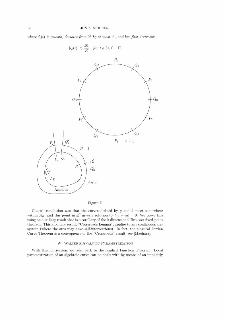
12 JON A. SJOGREN

where δi(t) is smooth, deviates from 0◦ by at most 1◦, and has first derivative

|ζi(t)| ⊂.01

Rfor t ∈ [0, 1]. �

P1

Q1

P0

Q0

P5

Q5

n = 3P4

Q4

P3

Q3

P2

Q2

R

Annulus

AR

P ′r

Q′r

Pr Qr

R+ 1

P ′0

Q′0

AR+1

Figure D

Gauss’s conclusion was that the curves defined by g and h meet somewherewithin AR, and this point in R2 gives a solution to f(x + iy) = 0. We prove thisusing an auxiliary result that is a corollary of the 2-dimensional Brouwer fixed-pointtheorem. This auxiliary result, “Crossroads Lemma”, applies to any continuous arc-system (where the arcs may have self-intersections). In fact, the classical JordanCurve Theorem is a consequence of the “Crossroads” result, see [Maehara].

W. Walter’s Analytic Parametrization

With this motivation, we refer back to the Implicit Function Theorem. Localparametrization of an algebraic curve can be dealt with by means of an implicitly

13

defined function such as F (x, y(x)) = 0 or F (x(y), y) = 0. With F a polynomial,one cannot expect the solution y(x), say to be polynomial. The right category tooperate in is that of real analytic functions (power series convergent in some openinterval). For example, the “nodal cubic” given by F (x, y) = y2 − x2(x + 1) hasa singularity at (0, 0), but can be defined near the Origin by means of two curves(“one-manifolds”) given by Y (X) = ±X

√X + 1.

At the “compactifying point” (−1, 0), a separate parametrization, of X in termsof Y , should be found in view of ∂F

∂Y= 2Y which equals 0 at (−1, 0), even though

the curve is smooth here. The square roots in the expressions above can be writtenas convergent power series. Certainly our starting data, the plane curves that ariseas real and imaginary parts of the complex polynomial P (z), form a special case of“power series” in two variables.

Thus we use a rather general implicit function theorem, following [Walter 1992].Let

f(x, y) =∑

aijxiyj , f(0, 0) = a00 = 0, fy(0, 0) = a01 6= 0

with aij , x and y belonging to R.

Proposition (Implicit Analytic Parametrization). Suppose that the seriesdefining f converges absolutely for |x| ≤ a, |y| ≤ b, with a, b > 0. Then there arereal numbers 0 < r ≤ a, 0 < s ≤ b and a power series w(x) converging absolutely for|x| ≤ r such that f(x,w(x)) = 0 for |x| ≤ r, |w(x)| ≤ s and furthermore f(x, y) 6= 0for all points (x, y) ∈ U ×W , not equal to one of the (x,w(x)).

Here U ×W denotes the rectangular box just constructed.The uniqueness of solution within the box is critical and may be called “Walter’s

Second Uniqueness”, the First being uniqueness merely among analytic solutioncurves. Actually “Second Uniqueness” depends upon carrying through Walter’sproof a second time, changing the Banach algebra of analytic “germs” to a Banachalgebra of locally bounded functions. We leave out this additional construction,but instead suggest alternative arguments that are consistent with an “analytic” orat least a smooth (differentiable) framework.

Sketch of proof of Proposition (see [Walter]). In the region of convergence wewrite f(x, y) = 0 in the form

Y =∞∑

i,j=0

bijxiyj := g(x, y)

where b00 = b0i = 0 and bij = −aij/a01. We already have the contraction operatorthat we need. Define Gw = g(x,w(x)) which we will see acts as an operator on areal Banach algebra H. Choose positive real numbers r, s according to the recipe

B =∞∑

i

|bi0|ri ≤1

2s

L =∞∑

i,j

|bij |rijsi−1 ≤ 1

2.

14 JON A. SJOGREN

Now let H = Hr be the vector space of all functions

u(x) =∞∑

r=0

αkxk

which are absolutely convergent for x = r, and define a norm on Hr as

‖u(x)‖ =∞∑

0

|αk|rk <∞.

It is required to prove that ‖ · ‖ on Hr is a legitimate norm, and Cauchy sequencesu1, u2, . . . , uf , . . . of series in Hr, converge to a series in Hr. Also, with the productuv of the series defining the Banach product, one computes

‖uv‖ =∑

k

rk

∣

∣

∣

∣

∣

∣

∑

i+j=k

αiβj

∣

∣

∣

∣

∣

∣

≤∑

k

rk∑

i+j=k

|ci||dj | = ‖u‖‖v‖.

Walter gives some basic facts about the Banach algebra Hr.

i) ‖xk‖ = rk, hence ‖1‖ = 1.

ii) u ∈ Hr implies uk ∈ Hr with ‖uk‖ = ‖u‖k, k = 0, 1, 2, . . .

iii) If {un} is a sequence in Hr such that∑

‖un‖ <∞, then

u =∑

un ∈ Hr and ‖u‖ ≤∑

‖un‖.

iv) The integration operator (Iu)(x) =∞∑

k=0

αkxk+1

k + 1maps Hr into itself and

satisfies ‖Iu‖ ≤ r‖u‖ with equality for u = 1.

One may compute that when ‖u‖, ‖v‖ ≤ s then

‖Gu−Gv‖ ≤ L‖u− v‖ ≤ 1

2‖u− v‖.

Since B = ‖G(0)‖, and given u ∈ Hr with ‖u‖ ≤ s,

‖G(u)‖ ≤ ‖G(0)‖+ ‖G(u)−G(0)‖ ≤ 1

2s+ L‖u‖ ≤ s,

we see that G maps the closed ball ‖u‖ ≤ s into itself. By the Banach Fixed-PointTheorem, there must exist a fixed element w under G, unique for this propertyamong elements w ∈ Hr. �

15

Proof of Inverse Function Theorem Let f : U → Cw be analytic and Df|pinvertible for p ∈ U . Defining F : U × Cw → Cw by

F (z, w) = f(z)− w .

Now∂F

∂z= f ′(z), so f ′(p) 6= 0 gives, from the above “Implicit” Function Theorem

a mapping g : V ⊂ Cw → U that is locally analytic. It follows that F (g(w), w) = 0for w ∈ V , in other words f(g(w)) = w. But also

F (g(f(z)), f(z)) = f ◦ g ◦ f(z)− f(z) = 0 ,

so g(f(z)) = z for z ∈ g(V ). Thus we have the two “inverse” properties requiredby the Inverse Function Theorem cited above as a Proposition. �

To conclude the Section, we mention Walter’s Second Uniqueness Property, thatis, the “point-wise” uniqueness of the solution w that we found. We repeat theproof above, this time working with the Banach algebra of bounded functions w :[−r, r] → R with norm ‖w‖ = sup{|w(x)| : |x| ≤ r}. This shows as in [Walter] thatour (bounded) analytic w gives rise to all the zeros of u(x, y) when |x| ≤ r, |y| ≤ s,namely they are exactly the pairs (x, w(x)). Since we have not covered the proof ofSecond Uniqueness in detail, those places where it is used in the continuation aregiven alternate treatment.

Regular Values and Curve Singularity

For the versions of Gauss I carried through on [Gersten-Stallings] and by J.Martin et al. in [MSS], it is a key point to have both components g, h in f(z) =g(x, y)+ih(x, y) = 0 lead to non-singular real algebraic curves g(x, y) = 0, h(x, y) =0 valid in a disk AR. Every point (x, y) should be a regular point for both g and h,where (x, y) is on the respective curve g = 0 or h = 0. This avoids self-intersectionof any component within AR of the curve, and for that matter any intersection oftwo components of g(x, y) = 0 (same for h(x, y)).

Since for each component G0, . . . , Gk−1,H0, . . . ,Hk−1 (as it will turn out), thereare only finitely many extrema, we can arrange for the “coordinate patches” of thiscomponent ηi : [tb, te] → R2, i = 0, . . . to contain at most one extremum. Therethen follows the condition K, also referred to as b) in the next Section, which is akey element of the curve construction in [Ostrowski]. At each “end” of η0, namelyη0(t0) and η0(t1) for the endpoints t0, t1 of the parametrizing interval, the functionη0(t) is monotone in both x and y coordinates. Thus definite limits

(K) limt→t+

0

η0(t) = η−0 , limt→t−

1

η0(t) = η+0 exist.

A similar property holds for all ηj . One may now use the Implicit Function Theoremto generate η1 : (t∗1, t2) → R

2 on a new interval, centered at u1 = η+0 and an openset V1 ⊂ R

2 containing u1, where uniqueness of the solution prevails.The absence of curve singularities is critical to the approach of [MSS] which

constructs a beautiful combinatorial structure on the curve components, leading toall n algebraic roots appearing at once, as intersection points. In our approach weare completely indifferent to self-intersections and intersections among components.

16 JON A. SJOGREN

We do need non-singularity (points on the curve are regular for g and for h) for onereason: the curve components must have distinct endpoints on the circle ER = ∂AR.This will force some component of G : g(x, y) = 0 to intersect some component ofH : h(x, y) = 0, yielding the one root z0 = x0 + iy0 for f(z) that we seek.

Since g and h are harmonic conjugates, the point sets

S ={

(a, b) ∈ R2 : gx(a, b) = gy(a, b) = 0

}

T ={

(a, b) ∈ R2 : hx(a, b) = hy(a, b) = 0

}

are the same. In fact this is the “same” as {z = a+ bi} where f ′(z) = 0, which ofcourse is finite by elementary field theory.

We wish both curves to be singularity-free, which means that for any (a, b) ∈S = T , we have g(a, b) 6= 0, h(a, b) 6= 0. If there exists z0 = a + ib with f(z0) =g(a, b) + ih(a, b) = 0, we have found a root and are done. But it might happenthat g(a, b) = 0 and h(a′, b′) = 0 for a 6= a′ or b 6= b′, (a′, b′) ∈ S. In that caseone or the other of g and h would potentially define a singular curve. Changingg(x, y) = 0 to g(x, y) = ǫ1, by a real constant small in modulus, we may assume thatg(x, y) := g(x, y)− ǫ1 never takes the value 0 ∈ R on any (a, b) ∈ S = set of critical

points {z0} of f(z). Similarly we may find ǫ2 near 0 such that h(x, y) := h(x, y)−ǫ2never satisfies h(a, b) = 0 for any a + ib ∈ “finite singular set of f(z)”. Then let

f(z) = f(z)− ǫ1 − iǫ2, which has the same set of critical points as does f(z).In summary, we wish to modify the complex equation f(z) = 0 so that g(x, y) = 0

does not have solutions (a, b) yielding f ′(a+ ib) = 0. The exact same constructionapplies to h(x, y).

Merely alter g to g by subtracting small positive or negative ǫ1. Now the newg might have acquired a new solution (a′, b′) where f ′(a′ + ib′) = 0. In that casepush all g to g by adding to g a real constant ǫ′1, smaller in modulus than ǫ1, so bynow we have avoided both “critical” solutions (a, b) and (a′, b′). After finitely manysteps we have (re-using notation) g(x, y) = g(x, y)+ ǫ where g(x, y) = 0 contains nosingularities. Again by closure of f(z), given that f(z) = 0 also has no solution, weconstruct ǫ, δ where f(z) = ǫ+ iδ has no solution, and its constituent real harmoniccurves g = 0, h = 0 have only regular points.

Admittedly the somewhat lengthy argument above is covered by [Gersten-Sta-llings] in one sentence. But the authors did not make explicit the need to assume,for the purposes of their argument, that both harmonic curves are non-singular.

We just established that there is a sequence {ǫk1} converging monotonically inmodulus to 0 ∈ R (where k is an index), such that g(a, b) = ǫk1 never has a solutionin S. Also we have a sequence {ǫk2} converging monotonically in modulus to 0 ∈ R

such that h(a, b) = ǫk2 never has a solution (a, b) ∈ S = T either. We claim thatif f(z) = 0 has no solution at all, then neither does f(z) = ǫ1 + iǫ2, for valuesǫ1, ǫ2 arbitrarily close in to 0 ∈ R. If such a convergent sequence did exists, withsolutions zk

f(zk) = ǫk1 + iǫk2 ,

the solutions would be bounded and a convergent sub-sequence of {zk} would leadto f(zk) = 0. Thus the Reich Principle shows that we can reduce the problem ofexistence of a root for f to one where the two real curves g(x, y) = 0 and h(x, y) = 0have no singularities in R2.

17

With these choices we now have in AR+1, that g−1(0) is a “smooth 1-manifold”,

consisting of several arcs with no intersections, and h−1(0) is also a “smooth 1-manifold” composed of non-intersecting arcs.

Furthermore g−1(0) ∩ h−1(0) is empty unless some x + iy in the intersectionsolves f(x + iy) = 0. We write g−1(0) instead of g−1(ǫ) as in [Gersten-Stallings]as we take it that the “ǫ modification” to the original polynomial function hasalready been carried through. The following Section will use the Implicit FunctionTheorem to describe the arc structure of g−1(0) within the disc AR. The boundarypoints of g−1(0) and h−1(0) on ER or ER+1 lie on a combinatorial configurationthat eventually will contradict g−1(0)∩ h−1(0) = ∅, and we will produce a solutionto f(z) = 0 ∈ Cw.

Inside the Disk AR

The next step is to characterize each arc in AR which is the continuation at Pior Qi of a given arc γi or ζi. Begin by considering the connected component G0 ofAR ∩ g−1(0) that contains the “node” P0. By means of the Implicit Function The-orem, since the entire curve g(x, y) = 0 is non-singular, it is possible at P0 to finda partial arc (coordinate patch) extending into AR and analytically diffeomorphic(expressible as a power series) to an open interval. We will denote by σ the full arcof a connected component G0, G1, . . . and by τ an arc of a component H0,H1, . . . .We denote generically by ηj a coordinate patch of one such arc or component. Sucha partial arc (patch) η0 (say open on G0 in the relative topology) and others subse-quent can be made small enough to have the following properties. See [Figure E].We may interpret η0 as a functional relation, with its graph [x, η0(x)] or [η0(y), y],or more generally [x(t), y(t)], for t ∈ (t0, t1), t0 < t1, η0(t) = u ∈ R2, x, y ∈ V , asmall open set containing u.

( ( ) )t0 t∗1 t1 t2

σ(t0)

σ(t1)

σ(t∗1)

σ(t2)

R

Figure E

(a) ηj has at most one y-extremum (maximum or minimum) in the parametriza-tion [x, y(x)] and at most one x-extremum in the parametrization [x(y), y].

(b) Unique limits exist for x(t), y(t) as t→ t−0 and t→ t+1 .(c) The {ηk} are ordered linearly with a non-empty overlap Im(ηi) ∩ Im(ηj)

only when i = j + 1 or j = i+ 1.

18 JON A. SJOGREN

Discussion of η conditions. Since our problem relates to the topology ofcurves in the plane, the intersection of g−1(0) and h−1(0), we may adjust thecoordinate system to gain any advantage through Algebra. In particular we wantg(x, y) as a polynomial form to contain no single-variable factors b(x) or c(y): thesewould present curve components parallel to an axis. This being given, the numberof extrema on g−1(0) should not be greater than 2n(n−1), as follows from Bezout’sTheorem [G. Fischer, Section 3.2].

Since g and h are continuous functions, we have that g−1(0) and h−1(0) are closedsubsets of AR. The connected component of g−1(0) containing P0 is constructed asabove by a sequence of arcs {ηi} coming from Walter’s Implicit Function Theorem.The arcs will eventually exhaust the allowable finite number of extrema. The “final”arc ηw will either “stop suddenly” in the interior of AR, or meet ∂AR. By “finalarc” we may mean a convergent sequence of monotone arcs. In either case one canconstruct a global parametrization of that part of the component G0 reached tothis point, as a concatenation, leaving in mind overlap of the local parametrizations{ηi} coming from Implicit Function Theorem. In the case where convergent “ends”of a sequence ηk, ηk+1, . . . converge to u∗ = (x∗, y∗) ∈ R2, we may take u∗ as thecenter of a new local parametrization η∗ : (t∞, t∞ + ǫ) → R

2. See [Figure F].The other possibility is that a ηj intersects the image of a previous ηi, i < j

or, a sequence ηj , ηj+1, . . . comes arbitrarily close to an image point of ηi, i < j.Specifically, the open set Vi, “domain of uniqueness” can be intruded on by patchesthat were generated subsequent to ηi.

...

P0

σ0 G0

convergent sequence

new arc

η∗

u∗

Figure F

Walter’s Second Uniqueness result, part of the analytic Implicit Function The-orem, rules out such behavior. If Di = {x, y : r1 < x < r2, s1 < y < s2} is thedomain of uniqueness for the patch ηi, then the only values (x, y) in Di that satisfyg(x, y) = 0 are the values ηi(t) = (x(t), y(t)) for t in the parametrizing interval(t∗i , ti+1). See [Figure G].

As previously remarked, this part of Walter’s Theorem requires considerationof a Banach algebra larger than “locally convergent power series”, namely “locallybounded functions”. It would be good to prove this uniqueness (a double point

19

or crossing is an algebraic singular point) without leaving the category of powerseries. For example, if ηj were to merge with ηk with an infinite order of tangency,

all higher order derivatives at u, namelydy

dx,d2y

dx2, . . . are equal for the two curves.

Thus by uniqueness of analytic solution the curves are equal in a neighborhood ofu. But u was assumed to be the first point for the parametrization that the curvesmeet (the curves are topologically closed) which gives a contradiction.

ηk ηk+1

convergent

η0

u∗

∂AR

Pk

ηw

AR

Figure G

u

ηj

ηk

Figure H

If on the other hand, ηj and ηk differ at u in some power of tangency, there areformulas that specify this “slope” or tangency, and there is no leeway for solutionsto the relation g(x, y) = 0 locally. For example if y = σ(x) is the solution at regularpoint x, y the slope there is given by the well-known formula

dy

dx

∣

∣

∣

∣

p=(x,y)

=dσ(x)

dx=

−gx(x, y)gy(x, y)

The formula for the second derivative is

d2y

dx2=

(

−g2ygxx + 2gxgygxy − g2xgyy)

g3y

20 JON A. SJOGREN

where

gxx =∂2g

∂x2, gxy =

∂2g

∂xdyetc.

There are formulas for all order derivatives, valid as long as gy 6= 0. This showsthe Taylor “jet” or “germ” at P is completely determined by g(x, y) as long as g isregular (surjective) at P . See [Figure H].

The above considerations have an essential consequence. Though we noted thatit is not vital for the rest of the proof whether G0 has any “self-intersections” orwhether Gi intersects Gj for i 6= j, it is essential that the starting node Pib ofGi be distinct from the ending node Pie , and that this pair be disjoint from anypair Pjb , Pje for i 6= j. We essentially did show that no self-intersection, mutualcrossings or mergings between Gi, Gj can occur, which is key to the “basketball”argument in [MSS].

A possible drawback of the reasoning about arcs given above is that either onemust work through a different “Walter” Uniqueness argument in a new category(bounded functions) or one must apply background knowledge about germs andjets of convergence power series. An alternative will now be sketched, that keeps usin the smooth category which is familiar to many. Taking by the argument about“finitely many extrema” of all the component curves G0, G1, . . . , Gk−1 (at least wesuspect that they are curves) we may look at an intersect or “merger” point isolatedin a rectangular box [Figure I]:

Γ ∆

box B

g

R

wp

Figure I

Now since p is regular for g(x, y), we can apply the Local Submersion Theoremof differential topology [Guillemin & Pollack, Section 1.4]. This is proved directlyfrom an Inverse Function Theorem that is available to us. Local submersion tellsus that there is a diffeomorphism ψ : B → T where T is another box but ψ(Γ) = L,where L is a horizontal segment. See [Figure J].

Γ∆

B

R2R2

p

T

L

a bψ

Figure J

21

But applying the same theorem to Γ + S, S a subset of the image of ∆ (“theother arc”) gives another diffeomorphism ϕ : B → T where ϕ(Γ) ⊆ L, but alsoϕ(g) ∈ L where g ∈ S. The diffeomorphism λ = ψϕ−1 : T → T takes L → L + S.The map λ is monotone on L and maps ψ(p) onto ϕ(p). Points in S converge top; therefore some λ−1(s) lies on the interval [λ(a), λ(b)]. But then λ−1(s) is notattained on t ∈ [a, b], contradicting the Intermediate Value Theorem.

Again, the “terminal” boundary point of K = Imσ must be some Pm distinctfrom P0 for the reasons just propounded. That is, σw would have to merge withσ0 at a previous coordinate σi(t

′), or meet P0 directly from inside AR. The σw(t)values near P0 would provide “extra solutions” to g(x, y) = 0 that are ruled out byWalter’s Second Uniqueness Theorem. Alternatively one can show the same, thatGi has two distinct endpoints of ∂AR, and these are distinct from those of all otherGj , by means of the derivative formulas and analytic uniqueness, or by the LocalSubmersion Theorem of differential topology.

We recapitulate the situation regarding algebraic arcs inside a closed disc AR.We quote C.F. Gauss (see [Smale]), “an algebraic curve can neither suddenly beinterrupted... nor lose itself after an infinite number of terms”.

From our point of view, the curve cannot “suddenly be interrupted” unless ∂ARis reached, since an extension of the growing arc can always be found at any limitpoint such a “u” discussed above. The curve cannot “lose itself” into oblivion likea logarithmic spiral, since the number of x- or y- extrema would have no bound.Arguments from compactness were not available until after Gauss’s time, but sucha proof using Bezout’s theorem would have been at hand.

So, according to Gauss, there remains the possibility that the curve “runs intoitself”, which we could rule out since we have enforced non-singularity of the curvecomponents. There remains only “runs out to infinity in both directions” (at dis-tinct angles), which means that each topological component such as Gi has twoboundary points on ∂AR.

The admission by Smale, Master of the high-dimensional Universe, that “it is asubtle point even today” why a real algebraic component g−1(0) cannot enter ARwithout leaving, makes one wonder whether all similar issues have been cleared upfor “3-folds in projective N -space” and so forth.

Pulling together the various pieces, we apply the process given above to allcomponents of G = g−1(0) ∩ AR and components of H = h−1(0) ∩ AR. We find,as is discussed in [Gersten-Stallings], [Uspensky] and [MSS] that there are n arcsG0, . . . , Gn−1, parametrized by {σi}, and n arcs H0, . . . ,Hn−1, parametrized by{τj}, connecting up the P0, . . . , P2n−1 and Q0, . . . , Q2n−1 respectively. In [FigureK] we see the “matching” partially defined by [0] ↔ [k] for P and [0] ↔ [m] for Q.

In the previous Section we saw that the collection of P -arcs {σi} in AR, eachcorresponding to a component Gi, were disjoint by the smoothness of the overallalgebraic curve g(x, y) = 0. Similarly the arcs {τj} corresponding to the compo-nents {Hi}, whose endpoints are {Qf} do not intersect. The goal now is to showthat some arc σj must meet some arc τk within AR.

22 JON A. SJOGREN

AR+1

Q′m

Pk

Pk

Qm

σ0

τ0

P ′k

P0P ′0

γ0

Q0

ξ0

Q′0

Figure K

We give the topological part of the short remaining argument.

Proposition [Maehara]. Suppose that a continuous arc σ on AR has distinctendpoints (nodes) E,F separated by nodes A,B, where E = [2e], F = [2f ], A =[2a + 1], B = [2b + 1] are the distinct boundary points of τ . Then σ and τ have acommon point (non-empty intersection) within AR. �

AR

B = Qb

F = Pf A = Qa

E = Pe

Figure L: Maehara Crossroads Theorem

Remarks. Note that σ and τ in this statement are not required to be simpleor smooth arcs, but each boundary ∂σ, ∂τ lies on ∂AR and consists of two points.“Separated” means that on the circle, reading counterclockwise the indicated nodessimilar to the following, see [MSS].

EQP Q PQ . . . APQP Q . . . FQPQPQ . . . BPQP . . .

23

orEQPQ . . . BPQP . . . FQPQ . . . APQP . . . ,

or a cyclic permutation of same.On the other hand the configuration EPQPFAQPQB does not satisfy the hy-

pothesis. In this case it is possible to choose σ and τ that do not intersect. See[Figures L & M].

A

B

F

E

τ

σ

Figure M

A generalization of Maehara’s result, deriving from the Theorem of Poincare-Miranda, is discussed in the Appendix. The article by three authors on “basketballconfigurations” [MSS] shows more strongly that every σi is matched to one τji withwhich it has exactly one intersection point. Their proof uses non-self-intersectionof G and H and a less elementary topological fact, the Jordan Curve Theorem (inits form applying to smooth curves).

Sector Matching by Harmonic Components

We review notation that has already been used, and is consistent with the treat-ment in [Uspensky, Appendix I], and similar to that of [MSS]. Consider 2N non-negative integers in an ordered interval

{2N} = [0, 1, . . . , 2N − 1].

Choosing say N = 5 and A = 3, B = 7 we obtain two sectors of {2N} − (A,B),namely S1 = [4, 5, 6] and S2 = [8, 9, 0, 1, 2] where we see that the integers wereactually in sequence mod (10). The model to keep in mind is the circle ER = ∂ARdescribed earlier where P0, . . . , P2N−1 were given in counter-clockwise order. Wemay say that 4 and 6 are in the same sector S1 for {2N} − (A,B) but that the“matched pair” (A,B) separates nodes 5 and 0. See [Figure N].

Getting to the case of interest, let N = 2n where n is the degree of our originalpolynomial P (z) (or f(z)). In this case our geometric labels look like

Q0 ∼ [0] Q1 ∼ [2] · · ·QN−1 ∼ [4n− 2]

P0 ∼ [1] P1 ∼ [3] · · ·PN−1 ∼ [4n− 1]

in the above description.

24 JON A. SJOGREN

The pairing of the boundary by arcs σj corresponding to Pj , and the boundarypoints of arcs τk corresponding to node Qk gives a matching (fixed-point free in-volution) of the {Pj}, and of the {Qk} respectively. Given some arc σ, its distinctend-nodes form two sectors I and II

A ∼ [k], [k + 1], . . . , B ∼ [m].

Hence, A and B are “P -nodes”. Suppose that the number of Q-nodes in sector Iis odd. See [Figure O].

Sector ISectorII

Pk Qk Pk+1 Qk+1 · · ·Pk+5

Qk+5· · ·

Figure N

Sector I

Sector II

P2Q1

P1

Q0

P0 ∼ [0]

Q7 ∼ [15]

P7 ∼ [14]

Q6P6

Q5

P5

Q4

P4

Q3

P3

Q2

τ1

σ0

Figure O: (P0, P3) gives Sector I = [Q0, P1, Q1, P2, Q2] and

Sector II = [Q3, P4, Q4, P5, Q5, P6, Q6, P7, Q7]

hence separates Q1 from Q4. If σ0 has boundary P0, P3, then τ1 with boundaryQ1, Q4 should intersect σ0.

25

Then one of the nodes Qf in Sector I must match (be attached by a τ arc) anode Q′

f of Sector II. By the Proposition of Maehara, this τ -arc must intersectthe original σ-arc in the interior of AR. So we would have a common solution(a, b) ∈ R2 for g(a, b) = h(a, b) = 0.

On the other hand, if the number of Q nodes in Sector I is even, we may assumethat all of their arc-pairings occur within Sector I, else we have a τ ′ that must meetσ as before. Any such Q-pairing, call it τ ′′, forms new sectors labeled III and IV ,one of which, say III, lies entirely within the P -sector I, hence is strictly smaller incardinality. Now we are interested in the P -nodes of Section III. As always underthis construction (when Sector Λ′ ends up strictly contained in Sector Λ), there isat least one P -node in Sector III. If the count of these P -nodes is odd, a pairingarc σ′ must arise that meets τ ′′ in a solution point. If we are still not finished,interchanging the roles of P and Q, g and h and so forth, leads by induction toa basic case of a singleton P - or Q-node that must be paired outside its sector,leading to a solution point.

Appendix: The “Crossroads Theorem” in Higher Dimensions

Maehara’s ‘Crossroads’ result generalizes from arcs in a disc or square, to “hy-percurves” of complementary dimension, transverse in a cube of the ambient di-mension.

If I = [−1, 1] is the closed double interval, we define Ik ⊆ In by

Ik = {|x1| ≤ 1, . . . , |xk| ≤ 1, xk+1 = 0, . . . , xn = 0}

and similarly Il ⊆ In by

Il = {x1 = 0, . . . , xl−1 = 0, |xl| ≤ 1, . . . , |xk| ≤ 1} .

Suppose we have mappings g : Ik → In, h : Ik+1 → In satisfying

g| ∂Ik = id∂Ik , h| ∂Ik+1= id∂Ik+1

.

Then we have

Proposition (Generalized Crossing Theorem). In this case there exist

s ∈ Ik, t ∈ Ik+1 such thatg(s) = h(t).

In other words, the image G = g(Ik) meets the image H = h(Ik+1) in at least onepoint.

Maehara’s result is when k = 1, n = 2. For example, consider an arc (a ‘path’) inI3 from A to Q (in red), and a surface within I3 whose boundary is the “equator”in blue, BCDE. Then the path and the surface must meet within closed I3. See[Figure P].

The proof is an immediate application of Miranda’s Theorem, a version of theBrouwer Fixed-Point Theorem originally proposed by Poincare. See [Miranda],[Vrahatis]. �

26 JON A. SJOGREN

We regard Brouwer’s FPT as a tool to be employed without hesitation. Proofsof the equivalent “non-retraction theorem”, due to Y. Kannai (see [Flanders]), C.A.Rogers, and Milnor-Asimov are elementary and lucid. Any of these approaches leadsto a modern proof of the Poincare-Miranda Theorem, the generalized CrossroadsTheorem (“topological transversality”) and a new proof of the result of Maehara,which he uses in turn to obtain a short proof of the Jordan Curve Theorem.

E

Q

D

B C

A

Figure P

27

References

J.R. Argand, Essay sur une maniere de representer le Quantites imaginaires dan les constructions

Geometriques, Nahu Press, 2010.

L.E.J. Brouwer, Beweis der Invarianz der Dimensionzahl, Math. Ann. 70 (1911), 161–165.F.S. Cater, An elementary proof that analytic functions are open mappings, Real Analysis Ex-

change 27 (2001/2002), no. 1, 389–392.J. Dugundji, Topology, Allyn and Bacon, Boston, 1966.C.H. Edwards, Advanced Calculus of Several Variables, Academic Press, New York, 1973.B. Fine and G. Rosenberger, The Fundamental Theorem of Algebra, Undergraduate Texts in

Mathematics, Springer-Verlag, New York, 1997.Harley Flanders, Differential Forms with Applications to the Physical Sciences, Academic Press,

New York, 1963.G. Fischer, Plane Algebraic Curves, AMS Press, Providence, 2001.C.F. Gauss, Demonstratio nova theorematis omnen functionem algebraicam rationalem integram

unius variabilis in factores reales primi vel secundi gradus resolvi posse, Thesis UniversitatHelmstedt. In Werke III (1799), 1–30.

S. Gersten and J. Stallings, On Gauss’s first proof of the Fundamental Theorem of Algebra, Proc.Amer. Math. Soc 103 (1988), no. 1, 331–332.

V. Guillemin and A. Pollack, Differential Topology, Prentice-Hall, Englewood Cliffs, 1974.E. Hille, Analytic Function Theory I, Ginn, Boston, 1962.Wl. Kulpa, The Poincare-Miranda Theorem, Amer. Math. Monthly 104 (1997), no. 6, 545–550.J.E. Littlewood, Every polynomial has a root, J. London Math. Soc. 16 (1941), 95–98.R. Maehara, The Jordan Curve Theorem Via the Brouwer Fixed Point Theorem, Amer. Math.

Monthly 91 (1984), no. 10, 641–643.J. Martin, D. Savitt and T. Singer, Harmonic Algebraic Curves and Noncrossing Partitions,

[MSS], Discrete Comput. Geom. 37 (2007), 267–286.J. Milnor, Topology from the Differentiable Viewpoint, [TFDV], The University Press of Virginia,

Charlottesville, Second printing, 1969.C. Miranda, Un’osservazione su un teorema di Brouwer, Boll. Unione Mat. Ital. 3 (1940), 527.

A. Ostrowski, Uber den ersten und vierten Gauss’schen Beweis des Fundamentalsatzes der Alge-

bra, in Gauss Werke Band X, Georg Olms Verlag, New York, 1973.D. Reem, The open mapping theorem and the fundamental theorem of algebra, Fixed Point Theory

9 (2008), 259–266.S. Reich, Notes and comments, Math. Mag. 45 (1972), 113.S. Smale, The Fundamental Theorem of Algebra and complexity theory, Bull. Amer. Math. Soc 4

(1981), no. 1, 1–3.R.L. Thompson, Open mappings and the fundamental theorem of algebra, Math. Mag. 42 (1970),

no. 1, 39–40.

J.V. Uspensky, Theory of Equations, McGraw-Hill, New York, 1948.M. Vrahatis, A short proof and a generalization of Miranda’s Existence Theorem, Proc Amer

Math Soc 107 (1989), no. 3.W. Walter, A useful Banach algebra, El. Math 47 (1992), 27–32.S. Wolfenstein, Proof of the fundamental theorem of algebra, Amer. Math. Monthly 74 (1967),

853–854.

Towson, Maryland