3778 IEEE TRANSACTIONS ON INFORMATION THEORY, VOL. 52, NO. 8, AUGUST 2006

Distortion Bounds for Broadcasting With BandwidthExpansion

Zvi Reznic, Member, IEEE, Meir Feder, Fellow, IEEE, andRam Zamir, Senior Member, IEEE

Abstract—We consider the problem of broadcasting a single Gaussiansource to two listeners over a Gaussian broadcast channel, with � channeluses per source sample, where � > 1. A distortion pair (D ;D ) is saidto be achievable if one can simultaneously achieve a mean-squared error(MSE) D at receiver 1 and D at receiver 2. The main result of this cor-respondence is an outer bound for the set of all achievable distortion pairs.That is, we find necessary conditions under which (D ;D ) is achievable.We then apply this result to the problem of point-to-point transmission overa Gaussian channel with unknown signal-to-noise ratio (SNR) and � > 1.We show that if a system must be optimal at a certain SNR , then, asymp-totically, the system distortion cannot decay faster than O(1=SNR). As forachievability, we show that a previously reported scheme, due to Mittal andPhamdo (2002), is optimal at high SNR. We introduce two new schemesfor broadcasting with bandwidth expansion, combining digital and analogtransmissions. We finally show how a system with a partial feedback, re-turning from the bad receiver to the transmitter and to the good receiver,achieves a distortion pair that lies on the outer bound derived here.

Index Terms—Distortion region, joint source–channel coding, lossybroadcasting.

I. INTRODUCTION

The broadcast channel, illustrated in Fig. 1, is a communicationchannel in which one sender transmits to two or more receivers [1].Suppose that we are given an analog source and a fidelity criterion,and we want to convey the source to both receivers simultaneously.The problem of joint source–channel coding for the broadcast channelis to find the distortion region which is the set of all simultaneouslyachievable distortion pairs (D1; D2) at the two receivers. For a generalsource, broadcast channel, and distortion measure, this problem is stillopen [2].

We investigate below an important special case, of transmittinga band-limited white Gaussian source over a band-limited whiteGaussian broadcast channel with squared-error distortion measure.Note that a Gaussian broadcast channel is a degraded broadcastchannel [1], and we shall say that receiver 1 is connected to the goodchannel and receiver 2 is connected to the bad channel. Also notethat this type of problem can be characterized by the parameter �. Incontinuous-time systems, we define �

�= Wc=Ws, where Wc is the

channel bandwidth and Ws is the source bandwidth. In discrete-timesystems, � is defined as the number of channel uses per source sample.Since band-limited continuous-time systems can be translated todiscrete-time systems, we shall use the discrete-time representation.We shall focus on the bandwidth expansion scenario, in which � > 1.

Manuscript received January 22, 2005; revised December 12, 2005. The ma-terial in this correspondence was presented in part at the 40th Annual AllertonConference on Communication, Control and Computing, Monticello, IL, Oc-tober 2002. The work of R. Zamir was supported by the Israel Academy ofScience under Grant ISF 65/01.

The authors are with the Department of Electrical Engineering–Systems, Tel-Aviv University, Ramat-Aviv 69978, Israel (e-mail: zvi.reznic@amimon.com;meir@eng.tau.ac.il; zamir@eng.tau.ac.il)

Communicated by Y. Steinberg, Associate Editor for Shannon Theory.Digital Object Identifier 10.1109/TIT.2006.878178

Fig. 1. Lossy transmission of a source through a broadcast channel.

Following Shannon’s theory, a trivial Cartesian outer bound on thedistortion region is given by D1 � R�1(�C1) and D2 � R�1(�C2),where

R(x) =1

2log

�2

x(1)

is the rate-distortion function of a Gaussian source with variance �2 (inbits per source sample) [1], and C1 and C2 are the individual point-to-point capacities (in bits per channel use) of the good and bad channels,respectively. In the case of � = 1, the trivial outer bound is achievedby analog transmission, i.e., by sending the source uncoded [3]. Thismeans that in this special case, there is no conflict between the needsof the two receivers, and both of them perform as if the needs of theother receiver could be ignored.

For the case of � > 1, Mittal and Phamdo [4] suggested a hybriddigital–analog scheme which achieves the distortion pair

(D1;D2) = (R�1((�� 1)C2 + C1); R�1(�C2)): (2)

Other schemes were developed for the case of � > 1, providing otherachievable distortion pairs [3], [5], [6]. However, no nontrivial outerbound (converse) on the distortion region was ever derived. The mainresult of this correspondence is such an outer bound. For deriving theouter bound we use an auxiliary random variable, similar to the oneused by Ozarow [7] for proving the converse for the Gaussian multipledescription problem. It follows from our outer bound that the distortionpair (2) is optimal in the limit of high signal-to-noise ratio (SNR).

Regarding an inner bound for the distortion region, we develop anew coding scheme which combines elements from the Mittal–Phamdoscheme together with a Wyner–Ziv source encoding and a broadcastchannel encoding. In addition, we outline a second scheme, that canbe thought of as a multidimensional extension of Chen and Wornell’sanalog error-correction scheme [3], making further use of analog trans-mission.

A variant of the problem above is the problem of sending a Gaussiansource over an additive white Gaussian noise (AWGN) channel, wherethe SNR is unknown except that SNR � SNRmin, where SNRmin isknown. Using our outer bound on the distortion region for the broad-cast channel, we prove that for any system, if SNRmin is high, and ifthe system is tuned to be optimal at SNRmin, then, as the SNR im-proves (but the transmitter is held fixed), the distortion cannot decayfaster than 1=SNR for all values of �. For comparison, we recall thatthe solution of R(D0) = �C is given by D0 = �2=(1 + SNR)�, andhence, the mean-squared error (MSE) of a collection of systems, eachoptimally designed for a different (high) SNR, decays as 1=SNR�. Wenote that for the case where the system is optimal at SNRmin, our resultis stronger than a previous result by Ziv [8], who showed that asymp-totically, the distortion cannot decay faster than 1=SNR2 for all valuesof �.

0018-9448/$20.00 © 2006 IEEE

IEEE TRANSACTIONS ON INFORMATION THEORY, VOL. 52, NO. 8, AUGUST 2006 3779

The correspondence is organized as follow: In Section II, we intro-duce the outer bound on the distortion region. In Section III, we provethe theorem and corollaries of Section II. In Section IV, we apply ourresults to the case of point-to-point communication over a channel withunknown SNR. In Section V, we introduce a coding scheme for broad-casting with bandwidth expansion. In Section VI, we introduce themodulo-lattice modulation, which makes further use of analog trans-mission. In Section VII. we analyze the performance of a system witha feedback, and in Section VIII, we conclude the correspondence.

II. OUTER BOUND ON THE DISTORTION REGION

In this section, we introduce the outer bound, which is the main re-sult of the correspondence. Before doing so, we note that in the gen-eral case of lossy broadcasting the distortion region depends only onthe marginal distributions of the channel (see Appendix I for proof).We recall that this is also the case for the channel coding problem ofbroadcast channels [1, p. 422].

We denote the source bySSS = (S1; . . . ; Sm), and the decoders outputby SSS111 = (S1;1; . . . ; S1;m) and SSS222 = (S2;1; . . . ; S2;m). We denotethe channel input by XXX = (X1; . . . ; Xn) and the channel outputs byYYY 1 = (Y1;1; . . . ; Y1;n) and YYY 222 = (Y2;1; . . . ; Y2;n). The bandwidthexpansion ratio � is defined by

� =n

m(3)

and we shall focus on the case where � > 1.

Definition 1: A Gaussian broadcast channel with input XXX and out-puts YYY 111 and YYY 222, satisfies for i = 1; 2

1

n

n

t=1

E X2

t � P;

Yi;t = Xt + Zi;t; Zi;t � N (0; Ni); t = 1; . . . ; n (4)

where ZZZ111 = (Z1;1; . . . ; Z1;n) and ZZZ222 = (Z2;1; . . . ; Z2;n) are memo-ryless and statistically independent of XXX , and N2 � N1.

The capacities C1 andC2 of the good and bad channel, respectively,are given by

Ci =1

2log 1 +

P

Nibits per channel use; i = 1; 2: (5)

We denote the distortion measure by d(SSS; SSSiii) for (i = 1; 2), anddefine the following.

Definition 2: (D1; D2) is an achievable distortion pair if, for any�� > 0, there exist integers m and n = �m, an encoding functionXXX = inm(SSS) and reconstruction functions SSS111 = gn1m(YYY 111) and SSS222 =gn2m(YYY 222), such that

E(d(SSS; SSSiii)) < Di + ��; for i = 1; 2: (6)

The achievable distortion region is defined as the convex closure of theset of achievable distortion pairs.

Note that it follows from Definition 2 that � is a rational number.This does not limit the scope of the results in any practical way, sinceany nonrational value could be replaced by a rational value which isarbitrary close to it.

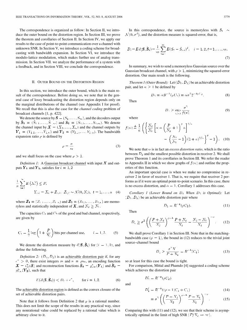
In this correspondence, the source is memoryless with St �

N (0; �2), and the distortion measure is squared-error, that is,

Di=Ed(SSS; SSSiii)=1

m

m

t=1

E(St � Si;t)2; i = 1; 2; t=1; . . . ;m:

(7)

In summary, we wish to send a memoryless Gaussian source over theGaussian broadcast channel, with � > 1, minimizing the squared-errordistortion. Our main result is the following.

Theorem 1 (Outer Bound): Let (D1;D2) be an achievable distortionpair, and let � � 1 be defined by

D2 = �R�1(�C2) = ��22�2�C : (8)

Then

D1 � sup�>0

�2

f(�)(9)

where

f(�)�=

1

�

N2

N1

� +P

N2

+ 1�

�1=�

�N2

N1

� 1 (1 + �)1=��

� 1 : (10)

We note that � is in fact an excess distortion ratio, which is the ratiobetweenD2 and the smallest possible distortion in receiver 2. We shallprove Theorem 1 and its corollaries in Section III. We refer the readerto Appendix II in which we show graphs of f(�) and outline the prop-erties of this function.

An important special case is when we make no compromise in re-ceiver 2 in favor of receiver 1. That is, we require that receiver 2 per-forms as if it were an optimal point-to-point scenario. In this case, thereis no excess distortion, and � = 1. Corollary 1 addresses this case.

Corollary 1 (Lower Bound on D1 When D2 is Optimal): Let(D1; D2) be an achievable distortion pair where

D2 = R�1(�C2): (11)

Then

D1 � �2P +N2

N2

��1P +N2

N1

�N2 �N1

N1

�1

: (12)

We shall prove Corollary 1 in Section III. Note that in the matching-bandwidth case (� = 1), the bound in (12) reduces to the trivial jointsource–channel bound

D1 ��2N1

P +N1

= R�1(C1) (13)

so at least for this case the bound is tight.For comparison, Mittal and Phamdo [4] suggested a coding scheme

which achieves the distortion pair

D0

2 = R�1(�C2)

and

D0

1 = R�1((�� 1)C2 + C1) (14)

= �2P +N2

N2

��1P +N1

N1

�1

: (15)

Comparing this with (11) and (12), we see that their scheme is asymp-totically optimal in the limit of high SNR (P=N2 ! 1).

3780 IEEE TRANSACTIONS ON INFORMATION THEORY, VOL. 52, NO. 8, AUGUST 2006

It can also be shown that in the limit of N2 ! 1, the lower boundof (12) becomes

D1 � �2 1 +�P

N1: (16)

In this case, one can actually achieve this bound by sending the sourceuncoded with power �P at 1=� of the time (first m samples of alength-n block), and sending zeros at the rest of the time (last n �msamples). Alternatively, if � is an integer, one can achieve this boundby repeating each source sample � times at a constant power P .

Corollary 2 addresses the special case in which we make no com-promise in receiver 1 in favor of receiver 2.

Corollary 2 (Lower Bound on D2 When D1 is Optimal): Let(D1; D2) be an achievable distortion pair where

D1 = R�1(�C1): (17)

Then

D2 � R�1(C2) 1�N1

N2+N1

N2

N1

P +N1

��1

: (18)

We shall prove Corollary 2 in Section III. For comparison, thescheme of Shamai, Verdú, and Zamir [5] (although not designedoriginally for broadcast channels) achieves the distortion pair

D1 = R�1(�C1); D2 = R�1(C2):

Hence, their scheme is optimal in the limit of N1=N2 ! 0.

III. PROOFS OF THEOREM 1, COROLLARY 1 AND COROLLARY 2

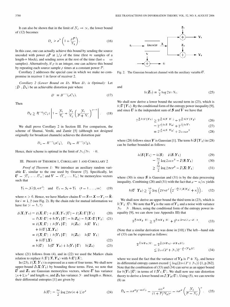
Proof of Theorem 1: We introduce an auxiliary random vari-able UUU , similar to the one used by Ozarow [7]. Specifically, letUUU = (U1; . . . ; Um) and VVV = (V1; . . . ; Vm) be memoryless vectorssuch that

Vt � N (0; ��2) and Ut = St + Vt (t = 1; . . . ;m) (19)

where � > 0. Hence, we have Markov chainsUUU$SSS$XXX$YYY i$ SSSifor i = 1; 2 (see Fig. 2). By the chain rule for mutual information wehave for (i = 1; 2)

I(XXX;YYY 111) = I(XXX;UUU) + I(XXX;YYY 111 jUUU)� I(XXX;UUU jYYY 1) (20)

= I(XXX;UUU) + h(YYY 111 jUUU)� h(ZZZ111)� I(XXX;UUU jYYY 111) (21)

= I(XXX;UUU) + h(YYY 111 jUUU)� h(ZZZ111)� h(UUU jYYY 111)

+ h(UUU jXXX;YYY 111)

= I(XXX;UUU) + h(YYY 111 jUUU)� h(ZZZ111)� h(UUU jYYY 111)

+ h(UUU jXXX) (22)

= h(UUU)� h(UUU jYYY 111) + h(YYY 111 jUUU)� h(ZZZ111) (23)

where (21) follows from (4), and in (22) we used the Markov chainrelation to replace h(UUU jXXX;YYY 111) with h(UUU jXXX).

In (23), I(XXX;YYY 111) is expressed as a sum of four terms. We shall nowupper-bound I(XXX;YYY 111) by bounding those terms. First, we note thatUUU and ZZZ111 are Gaussian memoryless vectors, where UUU has variance(�+1)�2 and lengthm, andZZZ111 has varianceN1 and length n. Hence,their differential entropies [1] are given by

h(UUU) =m

2log 2�e(�+ 1)�2 (24)

Fig. 2. The Gaussian broadcast channel with the auxiliary variable UUU .

and

h(ZZZ111) =n

2log 2�eN1: (25)

We shall now derive a lower bound the second term in (23), which ish(UUU jYYY 111). By the conditional form of the entropy power inequality [9],and since UUU is the independent sum of SSS and VVV we have that

2 h(UUU jYYY ) � 2 h(SSS jYYY ) + 2 h(VVV jYYY ) (26)

= 2 h(SSS jYYY ) + 2 h(VVV ) (27)

= 2 h(SSS jYYY ) + 2�e��2 (28)

where (28) follows sinceVVV is Gaussian [1]. The term h(SSS jYYY 111) in (28)can be further bounded as follows:

h(SSS jYYY 111) = h(SSS)� I(SSS;YYY 111) (29)

=m

2log 2�e�2 � I(SSS;YYY 111) (30)

�m

2log 2�e�2 � I(XXX;YYY 111) (31)

where (30) is since SSS is Gaussian and (31) is by the data processinginequality. Combining (28) and (31) with the fact that � = n=m yields

h(UUU jYYY 111) �m

2log 2�e�2 2� I(XXX;YYY ) + � : (32)

We shall now derive an upper bound the third term in (23), which ish(YYY 111 jUUU). We note that YYY 222 is the sum of YYY 111 and a noise with varianceN2 �N1. Hence, using the conditional form of the entropy power in-equality [9], we can show (see Appendix III) that

2 h(YYY jUUU) � 2 h(YYY jUUU) + 2log(2�e(N �N )): (33)

(Note that a similar derivation was done in [10].) The left—hand sideof (33) can be expressed as follows:

2 h(YYY jUUU) = 2 (h(YYY )�I(YYY ;UUU))

� 2�e(P +N2)2� I(YYY ;UUU) (34)

where we used the fact that the variance of YYY 222 is P + N2, and henceits differential entropy cannot exceed n

2log(2�e(P +N2)) [1, p.262].

Note that the combination of (33) and (34) can serve as an upper boundfor h(YYY 111 jUUU) in terms of I(YYY 2;UUU). We shall now use rate distortiontheory to derive a lower bound on I(YYY 222;UUU). Using (5), we can rewrite(8) as

D2 = ��22�2�C =��2

(1 + P=N2)�= ��2 N2

P +N2

�

: (35)

IEEE TRANSACTIONS ON INFORMATION THEORY, VOL. 52, NO. 8, AUGUST 2006 3781

We have

E(d(SSS2; UUU))=E1

m

m

t=1

(S2;t � Ut)2 (36)

=E1

m

m

t=1

(S2;t � St + St � Ut)2

(37)

=E1

m

m

t=1

(S2;t � St)2 + E

1

m

m

t=1

(St � Ut)2

(38)

=D2 + E1

m

m

t=1

V 2t (39)

=��2N2

P +N2

�

+ ��2 (40)

where (38) follows since St � Ut = Vt is independent of S2;t � St,(39) follows from (7) and (19), and (40) follows from (19) and (35).We now have

1

nI(YYY 2;UUU) �

1

nI(SSS2;UUU) (41)

�1

nmR(Ed(SSS2;UUU)) (42)

�1

2�log

(�+ 1)�2

��2 NP+N

�

+ ��2(43)

where (41) is by the data processing inequality, (42) is by rate-distortiontheory, and (43) follows since UUU is Gaussian with variance (�+ 1)�2,and by (1) and (40). Combining (33), (34), and (43) yields

h(YYY 111 jUUU) �n

2log 2�e(P +N2)

�� N

P+N

�

+ �

�+ 1

1=�

� 2�e(N2 �N1) : (44)

Hence, we have bounded all four terms in (23). Combining these terms,that is, combining (23), (24), (25), (32), and (44) yields (45) at thebottom of the page, for all� > 0. Algebraic manipulation of (45) yields

1

nI(XXX;YYY 111) �

1

2�log f(�) (46)

for all � > 0, where f(�) is defined in (10).By rate distortion theory, by the data processing inequality, and by

(46) we have that if (D1; D2) is achievable than

1

�R(D1) �

1

nI(XXX;YYY 111) �

1

2�log f(�) (47)

for all � > 0. Combining this with the rate distortion function (1) andtaking the supermum over all � > 0 proves the theorem.

Proof of Corrolary 1: By Theorem 1 we have thatD1 ��f(�)

forall � > 0, and in particular for � ! 0 (from above). By (11) and (8)

we have that � = 1. Combining this with Property 3 of f(�), which isdescribed in Appendix II, proves the theorem.

Proof of Corrolary 2: By Property 4 of f(�), which is describedin Appendix II, we have that

lim�!1

1

2log f(�) = �C1: (48)

Hence, the requirement set by (17) can be written as

R(D1) = lim�!1

1

2log f(�): (49)

Using (1), we can write (49) as

D1 = lim�!1

�2

f(�): (50)

Combining this with Theorem 1 yield that (D1; D2) may only beachievable if f(�1) � lim�!1 f(�) for all �1 > 0 (otherwise, therewould be a lower bound on D1 that contradicts (17)). By Properties 7and 5 this may only happen if � � �th. This means that �th is in facta lower bound on the excess distortion ratio which is possible whenreceiver 1 is optimal. Combining the definition of �th, (92) with (1),(5), and (8) proves the corollary.

IV. TRANSMISSION OVER CHANNELS WITH UNKNOWN SNR

We now turn to the issue of lossy transmission over a point-to-pointchannel with unknown SNR. Corollary 1 sets a lower bound on thedistortion D1, achieved at SNR of P=N1, given that the transmitter isoptimal at SNR of P=N2. Hence, by defining SNRmin

�= P=N2 and

SNR�= P=N1 and by (12) we prove the following corollary.

Corollary 3: For every � > 1, if a transmitter is designed to beoptimal at signal-to-noise ratio SNRmin and the actual signal-to-noiseratio is SNR, where SNR > SNRmin, then, the resulting distortionD( SNR) must satisfy

D(SNR) � � ��2

SNR� (1� o(1))

where � is independent of the actual SNR and is given by

� =1

SNRmin

��1

and o(1) ! 0 as SNRmin ! 1.

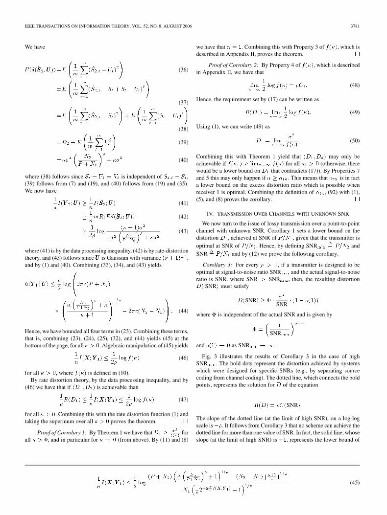
Fig. 3 illustrates the results of Corollary 3 in the case of highSNRmin. The bold dots represent the distortion achieved by systemswhich were designed for specific SNRs (e.g., by separating sourcecoding from channel coding). The dotted line, which connects the boldpoints, represents the solution for D of the equation

R(D) = �C(SNR):

The slope of the dotted line (at the limit of high SNR), on a log-logscale is��. It follows from Corollary 3 that no scheme can achieve thedotted line for more than one value of SNR. In fact, the solid line, whoseslope (at the limit of high SNR) is �1, represents the lower bound of

1

nI(XXX;YYY 111) �

1

2log

(P +N2)��

NP+N

�

+ 11=�

� (N2 �N1)�+1�

1=�

N11�2�2 I(XXX;YYY ) + 1

1=�(45)

3782 IEEE TRANSACTIONS ON INFORMATION THEORY, VOL. 52, NO. 8, AUGUST 2006

Fig. 3. MSE versus SNR. Solid line: the lower bound of Corollary 3. Dottedline: the solution of R(D) = �C(SNR).

Corollary 3. Thus, the MSE (SNR) behavior of any system, must beworse than what is represented by the solid line.

Note that in Corollary 3 we restricted the analysis to the case wherethe system is optimal at SNRmin, that is, when � = 1. We conjecturethat asymptotically, the distortion cannot decay faster than 1=SNR alsowhen the system is suboptimal at SNRmin, that is, when � > 1.

It is interesting to compare these results to a previous result of Zivwho analyzed the same problem [8]. In the case where the system isoptimal at SNRmin our result is stronger than Ziv’s result, since weshowed that the distortion cannot decay faster than 1=SNR, while Zivshowed that it cannot decay faster than 1=SNR2. (Although Ziv’s resultapplies even if the system is not optimal at any SNR.) Additionally, webounded the performance of any system, while Ziv restricted his resultto a class of systems, which he called “practical.”

V. INNER BOUND ON THE DISTORTION REGION

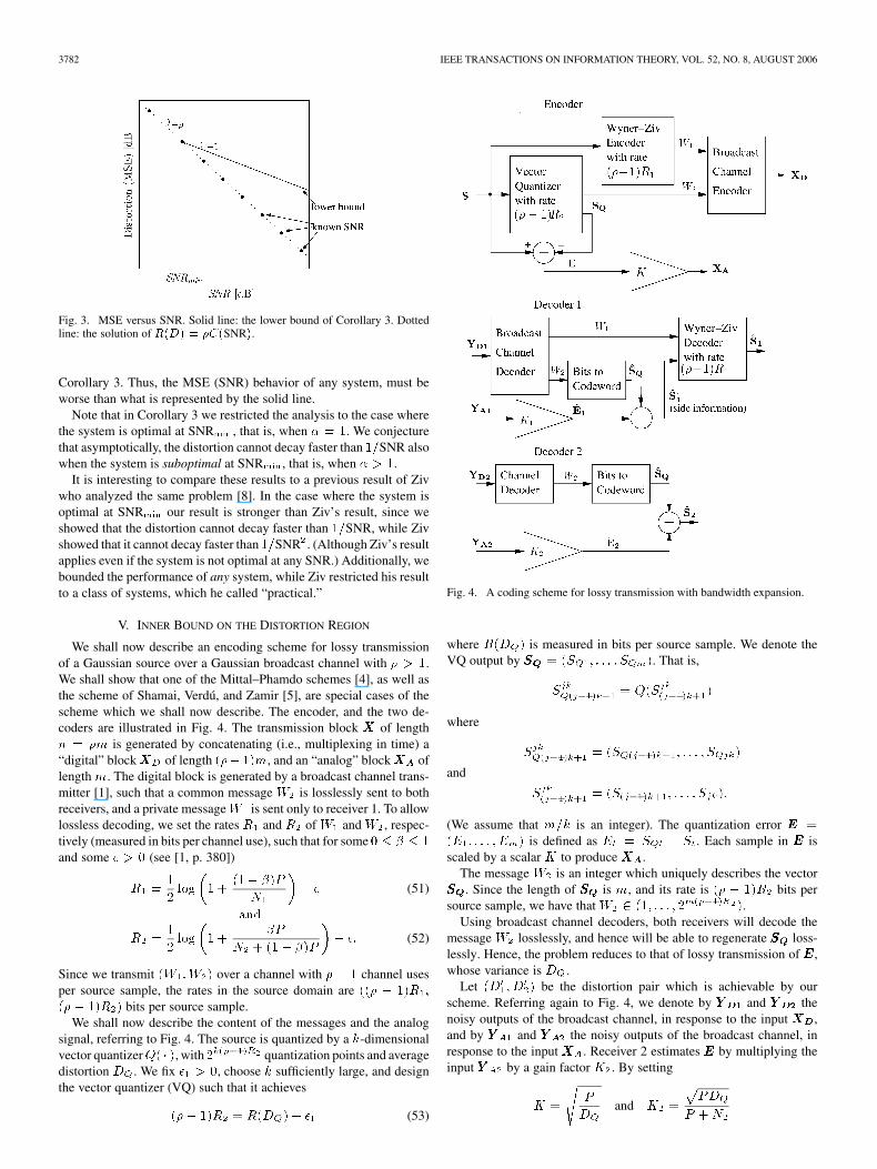
We shall now describe an encoding scheme for lossy transmissionof a Gaussian source over a Gaussian broadcast channel with � > 1.We shall show that one of the Mittal–Phamdo schemes [4], as well asthe scheme of Shamai, Verdú, and Zamir [5], are special cases of thescheme which we shall now describe. The encoder, and the two de-coders are illustrated in Fig. 4. The transmission block XXX of lengthn = �m is generated by concatenating (i.e., multiplexing in time) a“digital” blockXXXD of length (�� 1)m, and an “analog” blockXXXAAA oflength m. The digital block is generated by a broadcast channel trans-mitter [1], such that a common message W2 is losslessly sent to bothreceivers, and a private messageW1 is sent only to receiver 1. To allowlossless decoding, we set the rates R1 and R2 of W1 and W2, respec-tively (measured in bits per channel use), such that for some 0 � � � 1and some � > 0 (see [1, p. 380])

R1 =1

2log 1 +

(1� �)P

N1� � (51)

and

R2 =1

2log 1 +

�P

N2 + (1� �)P� �: (52)

Since we transmit (W1;W2) over a channel with � � 1 channel usesper source sample, the rates in the source domain are ((� � 1)R1;(� � 1)R2) bits per source sample.

We shall now describe the content of the messages and the analogsignal, referring to Fig. 4. The source is quantized by a k-dimensionalvector quantizerQ( � ), with 2k(��1)R quantization points and averagedistortion DQ. We fix �1 > 0, choose k sufficiently large, and designthe vector quantizer (VQ) such that it achieves

(�� 1)R2 = R(DQ) + �1 (53)

Fig. 4. A coding scheme for lossy transmission with bandwidth expansion.

where R(DQ) is measured in bits per source sample. We denote theVQ output by SSSQQQ = (SQ1; . . . ; SQm). That is,

SjkQ(j�1)k+1 = Q(Sjk(j�1)k+1)

where

SjkQ(j�1)k+1 = (SQ(j�1)k+1; . . . ; SQjk)

and

Sjk(j�1)k+1 = (S(j�1)k+1; . . . ; Sjk):

(We assume that m=k is an integer). The quantization error EEE =(E1; . . . ; Em) is defined as Et = SQt � St. Each sample in EEE isscaled by a scalar K to produce XXXAAA.

The message W2 is an integer which uniquely describes the vectorSSSQQQ. Since the length of SSSQQQ is m, and its rate is (� � 1)R2 bits persource sample, we have that W2 2 (1; . . . ; 2m(��1)R ).

Using broadcast channel decoders, both receivers will decode themessage W2 losslessly, and hence will be able to regenerate SSSQQQ loss-lessly. Hence, the problem reduces to that of lossy transmission of EEE,whose variance is DQ.

Let (D0

1; D0

2) be the distortion pair which is achievable by ourscheme. Referring again to Fig. 4, we denote by YYY DDD111 and YYY DDD222 thenoisy outputs of the broadcast channel, in response to the input XXXDDD ,and by YYY AAA111 and YYY AAA222 the noisy outputs of the broadcast channel, inresponse to the input XXXAAA. Receiver 2 estimates EEE by multiplying theinput YYY A2 by a gain factor K2. By setting

K =P

DQ

and K2 =PDQ

P +N2

IEEE TRANSACTIONS ON INFORMATION THEORY, VOL. 52, NO. 8, AUGUST 2006 3783

and taking the limit as � ! 0 and �1 ! 0 we have

D02 =

DQ

1 + PN

(54)

=N2

P +N2R�1((�� 1)R2) (55)

=�2N2

P +N22�2(��1)R (56)

=�2N2

P +N21 +

�P

N2 + (1� �)P

�(��1)

(57)

where (54) follows from standard MSE calculations (since the esti-mator of Et is scalaric and linear, its performance depends only onthe average of the variances of Et), (55) is by (53), (56) is by (1), and(57) is by (52).

As for the good receiver, we note that we can make use of the privatemessage W1 to further reduce the distortion. However, as a temporarystage, suppose that receiver 1 would estimate the source while com-pletely ignoring the private message. We shall denote this estimate bySSS�

111 . LetD�1 be the average distortion between SSS and SSS

�

111 . Repeating thesteps that led to (57) one can verify that

D�1 =

�2N1

P +N11 +

�P

N2 + (1� �)P

�(��1)

: (58)

Our problem with respect to decoder 1 reduces now to the following:the encoder needs to send a message W1, (at rate (� � 1)R1 bits persource sample) to the decoder, describing the source SSS, taking into ac-count that the decoder already has side information SSS

�

111 . This is in factthe Wyner–Ziv problem [11][12]. In Appendix IV, we prove a gen-eral upper bound on the quadratic Wyner–Ziv rate-distortion functionin terms of the MSE between the source and the side information. Inour case this bound asserts

RWZSSS j SSS

(x) �1

2log

1m

mt=1 E(St � S�

1;t)2

x

=1

2log

D�1

x(59)

where RWZSSS j SSS

( � ) is the Wyner–Ziv rate-distortion function of SSS givenside information SSS�

111 . Therefore, it is possible to design Wyner–Ziv en-coder and decoder with rate (� � 1)R1 bits per source sample thatachieves (as � ! 0)

D01 = D

�1 � 2

�2(��1)R

=�2N1

P +N11+

�P

N2+(1� �)P1+

(1� �)P

N1

�(��1)

(60)

where (60) follows from (51) and (58).Note that in the special case of � = 1 (R1 = 0), this scheme is the

same as one of the Mittal–Phamdo schemes [4]. On the other extreme,setting � = 0; (R2 = 0) reduces this scheme to the one of Shamai,Verdú, and Zamir [5]. Rewriting (60) and (57) in terms of � of (8),leads to the following theorem.

Theorem 2 (Inner Bound): For sending a Gaussian source withvariance �2 over the Gaussian broadcast channel, any distortion pair(D0

1; D02) of the form

D02 = �R

�1(�C2) = ��2 N2

P +N2

�

(61)

and

D01 � ��

2 N2

P +N2

��1N1

P +N1

� 1 +N2

N1�1=(��1)

� 1�(��1)

(62)

for some � > 1, is achievable.

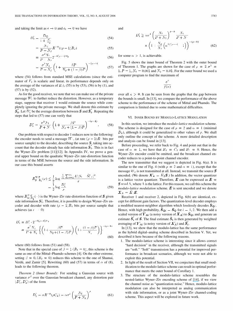
Fig. 5 shows the inner bound of Theorem 2 with the outer boundof Theorem 1. The graphs are shown for the case of � = 2; �2 =1; P = 1; N1 = 0:001 and N2 = 0:01. For the outer bound we used acomputer program to find the maximum of

�2

f(�)

over all � > 0. It can be seen from the graphs that the gap betweenthe bounds is small. In [13], we compare the performance of the abovescheme to the performance of the scheme of Mittal and Phamdo. Thecomparison is limited due to some mathematical difficulties.

VI. INNER BOUND BY MODULO-LATTICE MODULATION

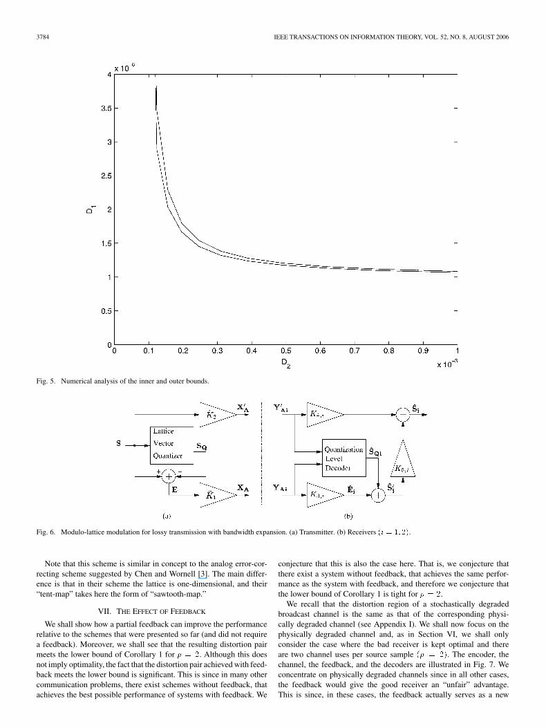
In this section, we introduce the modulo-lattice modulation scheme.The scheme is designed for the case of � = 2 and � = 1 (minimalD2), although it could be generalized to other values of �. We shallonly outline the concept of the scheme. A more detailed descriptionand analysis can be found in [13].

Before proceeding, we refer back to Fig. 4 and point out that in thecase of � = 1, we have that R2 = C2 and R1 = 0. Hence, theWyner–Ziv encoder could be omitted, and the broadcast channel en-coder reduces to a point-to-point channel encoder.

The new transmitter that we suggest is depicted in Fig. 6(a). It issimilar to the one of Fig. 4 (with � = 2 and � = 1), except that themessageW2 is not transmitted at all. Instead, we transmit the source SSSuncoded. (We denote XXX 0

AAA = ~K2SSS.) In addition, the vector quantizeris a lattice vector quantizer. Therefore, EEE can be expressed as EEE =SSSmod�, where� is the lattice. For this reason, we call this scheme themodulo-lattice modulation scheme. EEE is sent uncoded and we denoteXXXAAA = ~K1EEE.

Receiver 1 and receiver 2, depicted in Fig. 6(b) are identical, ex-cept for different gain factors. The quantization-level decoder employsa modified nearest-neighbor algorithm which losslessly decodes SSSQQQi.Hence, with high probability, SSSQQQiii = SSSQQQ for i = 1; 2. We then add ascaled version of YYY AAAiii (a noisy version ofXXXAAA) to SSSQQQiii and generate anestimate SSS

0

iii of SSS. The final estimate SSSiii is then generated by weightedaveraging of YYY 0

AAAiii (a noisy version of XXX 0AAA) and SSS

0

iii.In [13], we show that the modulo-lattice has the same performance

as the hybrid digital–analog scheme described in Section V. Yet, wedescribed it here because of the following reasons.

1. The modulo-lattice scheme is interesting since it allows correct“hard decision” in the receiver, although the transmitted signalsare “soft.” “Soft” transmission has a potential for improved per-formance in broadcast scenarios, although we were not able toexploit this potential.

2. In light of the result of Section VII, we conjecture that small mod-ification to the modulo-lattice scheme can result in optimal perfor-mance that meets the outer bound of Corollary 1.

3. The structure of the modulo-lattice scheme resembles thenested-lattice Wyner–Ziv encoding scheme of [14], if we viewthe channel noise as “quantization noise.” Hence, modulo-latticemodulation can also be interpreted as analog communicationwith side information, or as a joint Wyner–Ziv channel-codingscheme. This aspect will be explored in future work.

3784 IEEE TRANSACTIONS ON INFORMATION THEORY, VOL. 52, NO. 8, AUGUST 2006

Fig. 5. Numerical analysis of the inner and outer bounds.

Fig. 6. Modulo-lattice modulation for lossy transmission with bandwidth expansion. (a) Transmitter. (b) Receivers (i = 1; 2).

Note that this scheme is similar in concept to the analog error-cor-recting scheme suggested by Chen and Wornell [3]. The main differ-ence is that in their scheme the lattice is one-dimensional, and their“tent-map” takes here the form of “sawtooth-map.”

VII. THE EFFECT OF FEEDBACK

We shall show how a partial feedback can improve the performancerelative to the schemes that were presented so far (and did not requirea feedback). Moreover, we shall see that the resulting distortion pairmeets the lower bound of Corollary 1 for � = 2. Although this doesnot imply optimality, the fact that the distortion pair achieved with feed-back meets the lower bound is significant. This is since in many othercommunication problems, there exist schemes without feedback, thatachieves the best possible performance of systems with feedback. We

conjecture that this is also the case here. That is, we conjecture thatthere exist a system without feedback, that achieves the same perfor-mance as the system with feedback, and therefore we conjecture thatthe lower bound of Corollary 1 is tight for � = 2.

We recall that the distortion region of a stochastically degradedbroadcast channel is the same as that of the corresponding physi-cally degraded channel (see Appendix I). We shall now focus on thephysically degraded channel and, as in Section VI, we shall onlyconsider the case where the bad receiver is kept optimal and thereare two channel uses per source sample (� = 2). The encoder, thechannel, the feedback, and the decoders are illustrated in Fig. 7. Weconcentrate on physically degraded channels since in all other cases,the feedback would give the good receiver an “unfair” advantage.This is since, in these cases, the feedback actually serves as a new

IEEE TRANSACTIONS ON INFORMATION THEORY, VOL. 52, NO. 8, AUGUST 2006 3785

Fig. 7. Broadcasting with feedback.

observation of the source which is given to the good receiver. On theother hand, in physically degraded channels, the feedback conveys nonew information about the source (only new information about thereception at the bad receiver).

The encoder output block XXX of length n = 2m is a concatenationof two length-m blocks XXXaaa and XXXbbb, where XXXaaa = K�

1SSS and K�

1 =P=�2. Alternatively, we can write

Xa;t = K�

1St; t = 1; 2; . . . ;m: (63)

The channel is a physically degraded channel and therefore [1]

Ya1;t = Xa;t + Za1;t (64)

Ya2;t = Xa;t + Za1;t + Z 0

a;t; t = 1; 2; . . . ;m (65)

where Za1;t � N (0; N1) and Z 0

a;t � N (0;N2 � N1) and ZZZa1 andZZZ 0

a are memoryless and independent of each other and of XXX .The noisy signal Ya2;t returns as a feedback to the transmitter and to

receiver 1. The transmitter generates Xb;t by

Xb;t = K�

3 (S �K�

2Ya2;t); t = 1; 2; . . . ;m (66)

where K�

2 = P�

P+Nis the Wiener gain for receiver 2, and

K�

3 =(P +N2)P

N2�2

is a gain factor that scales Xb;t to have a power of P . As before, wehave

Yb1;t = Xb;t + Zb1;t (67)

Yb2;t = Xb;t + Zb1;t + Z 0

b;t; t = 1; 2; . . . ;m (68)

where Zb1;t � N (0;N1) and Z 0

b;t � N (0;N2 � N1) and ZZZb1 andZZZ 0

b are memoryless and independent of each other and of XXX .We shall now describe the operation of the two receivers. Let

YYY 222;ttt�=

Ya2;tYb2;t

and

YYY 111;ttt�=

Ya1;tYa2;tYb1;t

; t = 1; . . . ;m: (69)

(Recall that Ya2;t is the feedback.) The two receivers employ the fol-lowing optimal linear estimation of St. Let

RRRyyy;iii = E YYY tiii;ttt � YYY iii;ttt

and

rrrsssy;iii = E(StYYY iii;ttt): (70)

Combining (63)–(70) yields

RRRyyy;222 =P +N2 0

0 P +N2

rrrsssy;222 =

pP�2

N P�

P+N

(71)

RRRyyy;111 =

P +N1 P +N1P (N �N )pN (P+N )

P +N1 P +N2 0P (N �N )pN (P+N )

0 P +N1

(72)

and

rrrsssy;111 =

pP�2pP�2

N P�

P+N

: (73)

The linear estimation is given by

Si;t = aaatiii � YYY i;t; (74)

where

aaaiii = RRR�1yyy;iiirrrsssy;iii: (75)

The resulting distortion is then given by

Di = �2 � aaatiii � rrrsy;i: (76)

Combining (71)–(76) yields

D1 =�2N1N2

P 2 + 2PN2 +N1N2

and

D2 =�2N2

2

(P +N2)2: (77)

3786 IEEE TRANSACTIONS ON INFORMATION THEORY, VOL. 52, NO. 8, AUGUST 2006

Using the rate distortion function of a Gaussian source (1) and the ca-pacity of a Gaussian channel (5), one can verify that the distortion pairof (77) meets the lower bound of Corollary 1 for � = 2. We clarify thatthis does not imply optimality since the scheme assumed the existenceof a feedback, whereas the lower bound did not assume any feedback.Yet, we shall now explain the potential we see.

Shannon showed that feedback does not improve the capacity of apoint-to-point channel. There are other communication scenarios inwhich a feedback cannot improve the performance. We conjecture thatin our case as well, there exists a scheme that does not require a feed-back, and yields the same distortion pair as the one achieved with feed-back. This conjecture, combined with the result above leads us to con-jecture that the bound of Corollary 1 is tight for � = 2.

VIII. CONCLUSION

For lossy transmission of a Gaussian source over a Gaussian broad-cast channel with bandwidth expansion, we have derived inner andouter bounds on the set of all achievable distortion pairs (D1; D2), andshowed that one of the Mittal–Phamdo schemes is optimal at high SNR.The inner bound generalizes both the Mittal–Phamdo scheme and theShamai–Verdú–Zamir scheme.

Although the distortion in point-to-point communications is givenby D = �2=(1+ SNR)�, we showed that if a system must be optimalat a certain SNRmin, then asymptotically the distortion cannot decayfaster than 1=SNR.

APPENDIX ITHE DISTORTION DEPENDS ONLY ON THE CHANNEL’S MARGINALS

We shall now describe a general property of lossy broadcasting. Werecall that in the channel coding problem for broadcast channels, the ca-pacity region depends only on the marginal distributions of the channel[1, p. 422]. We shall show here that the same is true for the distortionregion in lossy broadcasting. We start with a definition.

Definition 3: A broadcast channel consists of an input alphabet Xand two output alphabets Y1 and Y2 and a probability transition func-tion fy ;y jx(yyy111; yyy222 jxxx), where xxx; YYY 111, and YYY 222 are of length n.

Now, suppose that we are given a source, a distortion measure, andtwo broadcast channels (with the same input and output alphabets), onewith probability transition function fy ;y jx(yyy111; yyy222 jxxx) and one withprobability transition function f�y ;y jx(yyy111; yyy222 jxxx), such that

fy jx(yyy111 jxxx) = f�y jx(yyy111 jxxx); for all YYY 111 2 Y1n and xxx 2 Xn

(78)

fy jx(yyy222 jxxx) = f�y jx(yyy222 jxxx); for all YYY 222 2 Y2n and xxx 2 Xn

(79)

but

fy ;y jx(yyy111; yyy222 jxxx) 6= f�y ;y jx(yyy111; yyy222 jxxx); for some (xxx; yyy111; yyy

222):

(80)

Now, using the notations of Definition 2, suppose that we arbitrarilychoose an encoder im(SSS) and decoders g1m(YYY 111) and g2m(YYY 222), andwe calculate the average distortion that result from the use of these de-coders. We denote by Df

i (i = 1; 2) the distortions in the case wherethe channel probability transition function is fy ;y jx(yyy111; yyy222 jxxx) and

by Dfi (i = 1; 2) the distortions in the case where the channel prob-

ability transition function is f�y ;y jx(yyy111; yyy222 jxxx). Then, the distortionscan be written for i = 1; 2 as follow:

Dfi =

SSS YYY

f(SSS) � fy jx(YYY iii j im(SSS))d(SSS; gim(YYY iii))dYYY iiidSSS

(81)

and

Dfi =

SSS YYY

f(SSS) � f�y jx(YYY iii j im(SSS))d(SSS; gim(YYY iii))dYYY iiidSSS:

(82)

Combining (78), (79), (81), and (82) yields

Df1; Df

2= Df

1; Df

2: (83)

It follows that any distortion pair that is achievable onfy ;y jx(yyy111; yyy222 jxxx) is also achievable on f�y ;y jx(yyy111; yyy222 jxxx) andvice versa. We therefore proved the following lemma.

Lemma 1: The distortion region depends on the broadcast channelprobability transition function fy ;y jx(yyy111; yyy222 jxxx) only through themarginal distributions fy jx(yyy111 jxxx) and fy jx(yyy222 jxxx).

An immediate conclusion from Lemma 1 is that the distortion regionof a stochastically degraded broadcast channel is the same as that of thecorresponding physically degraded broadcast channel.

APPENDIX IIPROPERTIES OF THE FUNCTION f(�)

We shall now outline the properties of the function f(�) (note that� > 0 by definition). Examples of f(�) are illustrated in Fig. 8.

Property 1: The function f(�) is continuous in �.

Property 2: If � > 1 then

lim�!0

f(�) =1: (84)

Property 3: If � = 1 then

lim�!0

f(�) =P +N2

N2

��1P +N2

N1

�N2 �N1

N1

: (85)

Property 4: In the limit of�!1, the function f(�) is independentof � and is given by

lim�!1

f(�) = 1 +P

N1

�

= 22�C : (86)

Property 5: The derivative of f(�) with respect to � is given by

@f(�)

@�=

g(�)

�2(87)

where

g(�) =h1(�)h2(�)

N�1

+ 1 (88)

IEEE TRANSACTIONS ON INFORMATION THEORY, VOL. 52, NO. 8, AUGUST 2006 3787

Fig. 8. f(�) for different values of �. Solid line: � = 1, dashed line: 1 < � < � (� = 2), dash-dot line: � > � (� = 6). The dotted line represents thelimit of f(�) as �!1, which is independent of �. (Parameters: P = 0:15; N = 0:01;N = 0:1; � = 3, and, therefore, � = 5:63).

where

h1(�) = N2�

�+ 1 +

P

N2

� 1=�

�(N2 �N1)1

�+ 1

1=� ��1

(89)

and

h2(�) = N2(��)�

�+ 1 +

P

N2

� 1=��1

+ (N2 �N1)1

�+ 1

1=��1

: (90)

Property 6: If follows from Property 5 that

lim�!1

@f(�)

@�= 0: (91)

Property 7: lim�!1 g(�) < 0 if and only if

� > �th�= 1 +

P

N2

��1N1

N2

N1

P +N1

��1

+N2 �N1

N2

(92)

where g(�) was defined in (88).

In the proof of Corollary 2 we show that �th is in fact a lower boundon the excess distortion ratio in receiver 2 in the case that receiver 1 isoptimal.

APPENDIX IIIPROOF OF EQUATION (33)

We shall now prove (33). Let

YYY0222�= YYY 111 +ZZZ

0 (93)

where ZZZ 0 = Z 01; . . . ; Z0n is memoryless with Z 0t � N (0;N2 � N1),

andZZZ 0 is independent ofUUU;XXX , andZZZ111. DefineZZZ 0 = ZZZ111+ZZZ0. Hence,

YYY0222 = XXX + ZZZ

0 where ZZZ 0 is memoryless, zero mean, Gaussian, withvariance N2, and independent of XXX . Additionally we have that

YYY 222 = XXX +ZZZ222 (94)

whereZZZ222 is also memoryless, zero mean, Gaussian, with variance N2,and independent ofXXX . Now, since we have Markov chainsUUU�XXX�YYY 222

and UUU � XXX � YYY0222, we conclude that f(yyy0222 juuu) = f(yyy222 juuu) for all

(uuu; yyy222; yyy0222) and therefore,

h(YYY 222 jUUU) = h(YYY 0222 jUUU): (95)

Now, by the conditional entropy power inequality [9], and since YYY 0222 isan independent sum of YYY 111 and ZZZ 0, and ZZZ 0 is Gaussian with varianceN2 � N1, we have

2 h(YYY jUUU) � 2 h(YYY jUUU) + 2log(2�e(N �N )): (96)

Combining (95) and (96) leads to (33).

APPENDIX IVON THE QUADRATIC WYNER–ZIV RATE DISTORTION FUNCTION OF

NON-GAUSSIAN VECTORS

We shall now prove a general upper bound on the quadraticWyner–Ziv rate-distortion function in terms of the MSE between thesource and the side information. Consider a source–side informationvector pair (SSS0; UUU 0) of length m, where SSS0 and UUU 0 are not necessarilyGaussian and not necessarily memoryless. The quadratic distortionbetween SSS0 and UUU 0 is defined as

d(SSS0; UUU 0)�=

1

m

m

t=1

E(S0t � U0t)2:

3788 IEEE TRANSACTIONS ON INFORMATION THEORY, VOL. 52, NO. 8, AUGUST 2006

We shall now show that for any such source–side information vectorpair (SSS0; UUU 0) the quadratic Wyner–Ziv rate-distortion function satisfies

RWZ

SSS jUUU (D) �1

2log

d(SSS0; UUU 0)

D(97)

where D is the allowed distortion.Proof: Let the pair (SSS�; UUU�) be Gaussian with the same

first- and second-order statistics as (SSS0; UUU 0), i.e., (SSS�; UUU�) �N (E(SSS0; UUU 0);Cov(SSS0; UUU 0)). Let ZZZ� be an independently distributedGaussian vector satisfying for every t

Var(S0t jS

0t + Zt ; U

0t) = D: (98)

We have

1

2log

d(SSS0; UUU 0)

D�

1

2m

m

t=1

logE(S0

t � U 0t)2

D(99)

� mina

1

2m

m

t=1

logE(S0

t � aU 0t)2

D(100)

= mina

1

2m

m

t=1

logE(S�

t � aU�t )

2

D(101)

=1

2m

m

t=1

logVar(St jUt )

D(102)

=1

2m

m

t=1

logVar(St jUt )

Var(S0t jS

0t + Zt ; U 0

t)(103)

�1

2m

m

t=1

logVar(St jUt )

Var(S�t jS

�t + Zt ; U�

t )(104)

=1

m

m

t=1

I(St ;S�t + Z�

t jU�t ) (105)

�1

m

m

t=1

I(S0t;S

0t + Z�

t jU0t) (106)

�1

mI(SSS0;SSS0 +ZZZ� jUUU 0) (107)

� RWZ

SSS jUUU (D): (108)

The preceding sequence of inequalities and equalities is now explained.Equation (99) follows by Jensen’s inequality, (100) follows as a = 1gives a larger value than the minimal a, (101) and (102) follow sincethe optimal square error in linear estimation is the same for Gaussianand non-Gaussian variables with the same second moments and equalsto the conditional variance, and (103) follows by the definition of ZZZ�.As for (104), it follows since Var(S�

t jS�t + Zt ; U

�t ), the Gaussian

conditional variance, equals the MSE of the best linear estimator of S0t

given S0t + Zt and U 0

t , which is larger than the optimal MSE of anyestimator given by the conditional variance of S0

t given S0t + Zt and

U 0t . Equation (105) follows directly from the expression of the mutual

information of Gaussian variables. To see (106), we have I(S0t ;St +

Zt jUt ) = h(St + Zt jUt )� h(Zt ), but

h(St + Zt jUt )

=1

2log [2�e(Var(St jUt ) + Var(Zt ))] (109)

�1

2log 2�e(Var(S0

t jU0t) + Var(Zt )) (110)

�1

2E log 2�e(Var(S0

t jU0t = u0) + Var(Zt )) (111)

= h(S0t + Zt jU

0t) (112)

where (109) follows from the definition of conditional entropy and thefact that Zt is independent of St ; Ut , (110) follows, as above, since

the non-Gaussian conditional variance is smaller than the Gaussianconditional variance, (111) is by Jensen’s inequality, and (112) comesfrom the definition of the conditional entropy, using the fact that Zt isindependent of S0

t; U0t . As for (107) we have

I(S0t;S

0t + Zt jU

0t) = h(S0

t + Zt jU0t)� h(Zt )

but since conditioning reduces entropy we have

h(S0t+Zt jU

0t)�h(S

0t+Zt jS

01; . . . ; S

0t�1; U

01; . . . ; U

0t ; . . . ; U

0m)

and so

m

t=1

h(S0t + Zt jU

0t) � h(SSS0 +ZZZ� jUUU 0)

while m

t=1h(Zt ) = h(ZZZ�). Finally, (108) follows since (107) rep-

resents the mutual information of a specific test channel that satisfiesthe distortion constrains, while RWZ

SSS jUUU (D) is the minimal mutual in-formation over all possible tests channels.

Note that we can show by a straightforward extension of the proof ofthe direct part of the Wyner–Ziv coding theorem, that for any stationaryand ergodic source, the vector form of the Wyner–Ziv function can bearbitrarily approached by a coding system operating on “super sourcesymbols.” Hence, it is possible to design an encoder–decoder pair withrate 1=2 log d(SSS0; UUU 0)=D and distortion D.

REFERENCES

[1] T. M. Cover and J. A. Thomas, Elements of Information Theory. NewYork: Wiley, 1991.

[2] M. D. Trott, “Unequal error protection codes: Theory and practice,” inProc. IEEE Information Theory Workshop, Haifa, Israel, Jun. 1996, p.11.

[3] B. Chen and G. Wornell, “Analog error-correcting codes based onchaotic dynamical systems,” IEEE Trans. Commun., vol. 46, no. 7, pp.881–890, Jul. 1998.

[4] U. Mittal and N. Phamdo, “Joint source-channel codes for broadcastingand robust communication,” IEEE Trans. Inf. Theory, vol. 48, no. 5, pp.1082–1103, May 2002.

[5] S. Shamai (Shitz), S. Verdú, and R. Zamir, “Systematic lossy source-channel coding,” IEEE Trans. Inf. Theory, vol. 44, no. 2, pp. 564–579,Mar. 1998.

[6] V. A. Vaishampayan and S. I. R. Costa, “Curves on a sphere: Errorcontrol for continuous alphabet sources,” in Proc. IEEE Int. Symp. In-formation Theory, Lausanne, Switzerland, Jun./Jul. 2002, p. 376.

[7] L. Ozarow, “On a source-coding problem with two channels and threereceivers,” Bell Syst. Tech. J., vol. 59, no. 10, pp. 1909–1921, Dec.1980.

[8] J. Ziv, “The behavior of analog communication systems,” IEEE Trans.Inf. Theory, vol. IT-16, no. 5, pp. 587–594, Sep. 1970.

[9] N. Blachman, “The convolution inequality for entropy powers,” IEEETrans. Inf. Theory, vol. IT-11, no. 2, pp. 267–271, Apr. 1965.

[10] Z. Reznic, R. Zamir, and M. Feder, “Joint source-channel coding of aGaussian-mixture source over the Gaussian broadcast channel,” IEEETrans. Inf. Theory, vol. 48, no. 3, pp. 776–781, Mar. 2002.

[11] A. D. Wyner and J. Ziv, “The rate-distortion function for source codingwith side information at the decoder,” IEEE Trans. Inf. Theory, vol.IT-22, no. 1, pp. 1–10, Jan. 1976.

[12] A. D. Wyner, “The rate-distortion function for source coding with sideinformation at the decoder—II: General sources,” Inf. Contr., vol. 38,pp. 60–80, 1978.

[13] Z. Reznic, “Broadcasting analog sources over Gaussian channels,”Ph.D. dissertation, Tel-Aviv Univ., Tel-Aviv, Israel, Aug. 2003.

[14] R. Zamir, S. Shamai (Shitz), and U. Erez, “Nested linear/lattce codesfor structural multiterminal binning,” IEEE Trans. Inf. Theory, vol. 48,no. 6, pp. 1250–1276, Jun. 2002.