Embed Size (px)
Citation preview
A COUPLED MAGNETOELASTIC MODEL FOR FERROMAGNETIC
MATERIALS
ANOUAR BELAHCEN1, KATARZYNA FONTEYN1, STEFANIA FORTINO2, REIJO KOUHIA2
1 Laboratory of Electromechanics, Helsinki University of TechnologyP.O. Box 3000, 02015 HUT, Finland
e-mail: [email protected], [email protected]
2Laboratory of Structural Mechanics, Helsinki University of Technology,P.O. Box 2100, 02015 HUT, Finland
e-mail: [email protected], [email protected]
ABSTRACT
This paper presents a coupled magnetoelastic model for isotropic ferromagnetic materials usedin electrical machines. As proposed by Dorfmann et al. for general nonlinear magnetoelastic solids,the constitutive equations of the model are written on the basis of the Helmholtz free energy forwhich the strain tensor and the magnetic induction vector are chosen as the basic variables. Asa result of the method, a suitable form of the free energy is chosen by comparing the proposedconstitutive relations and the corresponding experimental data under several external magneticfields and pre-stresses.
1 INTRODUCTION
The ferromagnetic materials can show the well known phenomenon of magnetostriction and arecharacterized by a coupled magnetomechanical field. In the traditional models for magnetostrictionthe constitutive equations of the material (linear or nonlinear) are decoupled [1].
Nowadays the so–called magnetoelastic coupling is widely used for modeling the reciprocal effectbetween the magnetic and the elastic field. In particular, the linear elastic behaviour is usually con-sidered, while the magnetic properties can be linear or nonlinear. Very simple magnetoelastic modelsare defined by using the magnetic forces as loads for the elastic field (weak coupling, see refs in [2]).In these coupling models the magnetic equations and the mechanical equations are solved separately.More accurate models, based on the so–called strong coupling ([3], [4], [5]), solve simultaneously thegoverning equations of the problem in the following coupled cases: i) linear magnetic - linear elasticfields, ii) nonlinear magnetic - linear elastic fields and iii) nonlinear magnetic - nonlinear elasticfields. The recent literature concerning the development of coupling magnetomechanical methods,pointed out that there is still a lack of both theoretical and experimental work in the developmentof constitutive relations of ferromagnetic materials (see [6] and [7]). As observed by Belahcen in[2], the knowledge of the coupled constitutive equations in general magnetostrictive materials is notpossible without measurements needed to provide the required material parameters.
In this paper, starting from the model proposed by Dorfmann et al. ([8], [9],[10]) for generalnonlinear magnetoelastic solids, the constitutive equations of isotropic ferromagnetic materials arewritten on the basis of the Helmholtz free energy. The strain tensor and the magnetic inductionvector are chosen as the basic variables. Following Dorfmann et al., since the Cauchy stress tensor isnot in general symmetric, the so–called total stress tensor, symmetric and defined as a function of theCauchy stress tensor and of the magnetic field vector, is introduced. In the general case of isotropicmagnetoelastic solids, the Helmholtz free energy depends on the six invariants, forming the integrity
basis of an isotropic tensor function depending on a symmetric second order tensor and a vector. Inthis work a suitable form of the Helmholtz free energy for isotropic ferromagnetic materials used inelectrical machines is then proposed by fitting the experimental data obtained by means of a simplebut sufficiently accurate measurement device. The measurement set-up enables measurements ofboth magnetization and magnetostriction as functions of the externally applied stress. As numericalresults, the magnetostriction curves for uniaxial problems under several external magnetic fields andpre-stresses are shown.
2 Governing equations for ferromagnetic materials
Let us consider a general electromagnetic body of domain Ω and boundary S subjected to bodyforces f in Ω and to surface forces t on S. Following Maugin [1], the mechanical balance laws of thebody are:
ρ+ ρ div u = 0 (1)ρ u = div σ + ρ f + fem (2)
where ρ is the mass density, u the displacement vector, (.) represents the total time derivativeoperator ( d
dt ), σ is the Cauchy stress tensor and fem the electromagnetic force (per unit volume).Equations (1) and (2) represent the conservation of mass and the balance of linear momentumequation, respectively.
The integral form of the energy balance equation in the isothermal case is written as
ddt
∫
Ω
(1
2ρu · u + ρU
)dΩ =
∫
Ω
(Φ + f · u) dΩ +∫
S
t · u dS (3)
where U represents the internal energy density per unit mass and Φ is the electromagnetic energydensity. In particular:
Φ =1
2E · D +
1
2B ·H (4)
where E is the electric field vector, D the electric displacement field vector, B the magnetic inductionfield vector and H the magnetic field intensity vector. The vector fields E,D,B and H obey to theMaxwell equations for general electromagnetic bodies (see [1]). Furthermore, B and H are relatedthrough
B = µ0(H + M) (5)
where µ0 is the magnetic permeability in the vacuum and M represents the magnetization. By usingthe mechanical balance laws (see Maugin [1]), equation (3) can be simplified as follows:
∫
Ω
ρ U dΩ =∫
Ω
(Φ + ε : σ) dΩ (6)
where ε is the infinitesimal strain tensor.
2.1 Case of quasi–magnetostatic of insulators
Let us now consider the assumption of quasi–magnetostatic of insulators (see [1]), which reducesthe Maxwell equations for general electromagnetic bodies to
div B = 0 (7)curlH = 0 (8)
In particular, (7) describes the conservation of magnetic flux and (8) the Ampere law in the sta-tionary case and null current density.
The assumption of quasi–magnetostatic of insulators reduces the balance equation (6) to∫
Ω
ρU dΩ =∫
Ω
(B ·H + ε : σ) dΩ (9)
Following Dorfmann et al., let us further assume the existence of a Helmholtz free energy ψ =ψ(ε,B) for which the strain tensor ε and the magnetic induction vector B are chosen as the basicvariables. In particular, in the case of isotropic ferromagnetic materials, ψ depends on the set ofinvariants
I1 = trε, I2 = tr ε2, I4 = B · B, I5 = B · ε ·B, I6 = B · ε2 ·B (10)By using the Clausius-Duhem inequality (see [1]), the constitutive equations of the material areexpressed as
σ = ρ∂ψ
∂ε(11)
M = −ρ ∂ψ∂B
(12)
It is worth to note that the Cauchy tensor σ is symmetric only when the magnetization M iseverywhere parallel to B (see [1], [8], [9], [10]). This is the case of the linear isotropic bodies, forwhich equation (12) reduces to
M = γB (13)with γ = (µ − 1)/(µµ0) where µ ≥ 1 represents the magnetic permeability. The proportionalitybetween M and B implies the independency of the free energy on the invariants I5 and I6. Actuallyin real ferromagnetic bodies, the magnetic permeability of the material depends not only on themagnetic field strength but also on the mechanical stress, i.e. on the solution of the elastic field.Then, in general cases, γ can be defined as a function of the invariants I4, I5 and I6. Furthermore,to avoid the use of a non-symmetric stress tensor, the so–called total stress tensor is defined:
τ = σ + µ−10
[BB− 1
2(B ·B)I
]+ (M ·B)I −BM (14)
where the dyad BB represents the open product, expressed in the component form as BiBj . Byusing (5) and in the absence of mechanical volume forces, equation (2) becomes:
divτ = 0 (15)
This expression is obtained by incorporating the electromagnetic force fem into the Cauchy stresstensor as a Maxwell stress (see [10]).
3 Proposed form of the Helmholtz free energy
Let us write the Helmholtz free energy ψ in terms of the invariants I1, I2, I4, I5 and I6 in thefollowing form:
ρψ =1
2λI2
1 + µI2 +1
2γ4I4 +
1
2γ5I5 +
1
2γ6I6 (16)
where λ and µ represent the Lame coefficients, the coefficient γ4 is a polynomial expansion of theinvariant I4
γ4 = γ(0)4 +
1
2γ
(1)4 I4 +
1
3γ
(2)4 I2
4 +1
4γ
(3)4 I3
4 +1
5γ
(4)4 I4
4 + ... (17)
while the coefficients γ5 and γ6 are constants.The constitutive equations of the model are then:
σ = λI1I + 2µε +1
2γ5 BB +
1
2γ6(B ε · B + B · εB) (18)
M = −γ′
4B − γ5 ε · B− γ6ε2 ·B (19)
whereγ
′
4 = γ(0)4 + γ
(1)4 I4 + γ
(2)4 I2
4 + γ(3)4 I3
4 + γ(4)4 I4
4 + ... (20)Then, the total stress tensor (15) has the following form:
τ = (λI1 − 12µ
−10 I4 − γ4I4 − γ5I5 − γ6I6)I + 2µε +
(µ−1
0 + γ′
4 + 12γ5
)BB+
+ 12 (γ5 + γ6) (B ε · B + B · εB) + 1
2γ6 (B ε2 ·B + B · ε2 B)(21)
3.1 Uniaxial case
In this work we consider the uniaxial case, such that
τ11 = τ ; otherwise τij = 0ε11 = ε1; ε22 = ε33 = ε2; otherwise εij = 0 (22)
B = [B1 0 0 ]T (23)
where the indexes 1, 2, 3 refer to the axes x1, x2, x3, respectively.The uniaxial model furnishes the following system of equations quadratic in ε1:
τ = λ(ε1 + 2ε2) + 2µε1 +(
12µ
−10 + 1
2γ5 + γ6ε1)B2
1
0 = λ(ε1 + 2ε2) + 2µε2 −(
12µ
−10 + γ
′
4 + γ5ε1 + γ6ε21
)B2
1
(24)
One of the solutions of the system represents the expression of the magnetostrictive strain in thedirection of the x1 axis which, after some manipulations, can be written as
ε1 = −1
4νξ6b1
β
[1 −
[1 +
8νξ6b1β2
( τE
−1
2(1 + 2ν + 4νξ4 + ξ5)b1
)]1/2]
(25)
with β = 1 + (2νξ5 + ξ6)b1 where b1 = µ−10 B2
1/E. Furthermore ξ4 = ξ(0)4 + ξ
(1)4 I4 + ξ
(2)4 I2
4 +ξ(3)4 I3
4 + γ(4)4 I4
4 . Note that ξ(i)4 = γ(i)4 µ0 (i = 0, 1, 2, 3, 4), ξ5 = γ5µ0 and ξ6 = γ6µ0 are dimensionless
parameters to be evaluated by fitting the experimental data in terms of magnetostrictive strains,magnetic field values and magnetic induction field values. Finally, ν is the Poisson’s ratio and Ethe Young’s modulus.
Note that, by neglecting the dependence of the Helmholtz free energy on the invariant I6, system(24) becomes linear in ε1 and the expression of the magnetostrictive strain in the direction of thex1 axis reduces to:
ε1 =1
1 + 2νξ5 b1
[ τE
−1
2(1 + 2ν + 4νξ4 + ξ5) b1
](26)
4 Some results
4.1 Measurements of magnetostriction
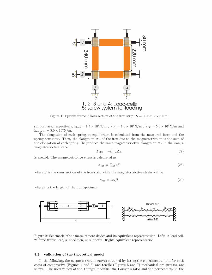
The experiments for measuring the magnetization and the magnetostriction data were conductedat the Laboratory of Electromechanics (Helsinki University of Technology, Finland). To obtain thedata as function of both the magnetic induction field and the external mechanical stress, a slightlymodified version of the 25 cm Epstein frame was used (see Figure 1). The modifications mainlyinvolve the dimensions of the test specimen and the use of extra insulation between strips (see[2] for the details). The screw system allowed for the application of both tensile and compressivemechanical stresses. The use of plastic strips between the iron strips prevented them bending whencompressive stress was applied. The measurement of magnetostriction was conducted by using thesame set-up as for the measurement of magnetization. The only difference is a piezoelectric forcetransducer introduced between the load cell and the specimen holder. The transducer was used forthe measurement of the force due to magnetostriction in the direction of the magnetic field.
As described in [2], the device for measuring magnetostriction furnishes a force from which themagnetostriction and the magnetostrictive stress need to be calculated. In particular, one strip of themeasurement device with its supports and holders, can be schematized as shown in Figure (2). Thispart is mechanically equivalent to the system of springs shown in the same figure. The force measuredby the piezoelectric force transducer is the force in the system of springs at equilibrium after themagnetostriction takes place. Since the measurement is made at a frequency of 5 Hz, the mass effectcan be ignored. The spring constants of the iron strip, the force transducer, the load cell and the
1
2
3 4
5
5
5 5
34
0 m
m
22
0 m
m
30
mm
1, 2, 3 and 4: Load-cells5: screw system for loading
Figure 1: Epstein frame. Cross section of the iron strip: S = 30 mm× 7.5 mm.
support are, respectively, kiron = 1.7× 10⁸N/m , kFT = 1.0× 10⁸N/m , kLC = 5.0× 10⁸N/m andksupport = 5.0 × 10⁶N/m.
The elongation of each spring at equilibrium is calculated from the measured force and thespring constants. Then, the elongation ∆u of the iron due to the magnetostriction is the sum ofthe elongation of each spring. To produce the same magnetostrictive elongation ∆u in the iron, amagnetostrictive force
FMS = −kiron∆u (27)
is needed. The magnetostrictive stress is calculated as
σMS = FMS/S (28)
where S is the cross section of the iron strip while the magnetostrictive strain will be:
εMS = ∆u/l (29)
where l is the length of the iron specimen.
3 2 1
4
44
kiron kFT kLC ksupport
Before MS
After MS
Figure 2: Schematic of the measurement device and its equivalent representation. Left: 1: load cell,2: force transducer, 3: specimen, 4: supports. Right: equivalent representation.
4.2 Validation of the theoretical model
In the following, the magnetostriction curves obtained by fitting the experimental data for bothcases of compressive (Figures 4 and 6) and tensile (Figures 5 and 7) mechanical pre-stresses, areshown. The used valued of the Young’s modulus, the Poisson’s ratio and the permeability in the
0 2 4 6 8 10 12 14 16 180
0.2
0.4
0.6
0.8
1
1.2
1.4
1.6
1.8
2
H1 (kA/m)
B1
(Tes
la)
...experimental results, − proposed model
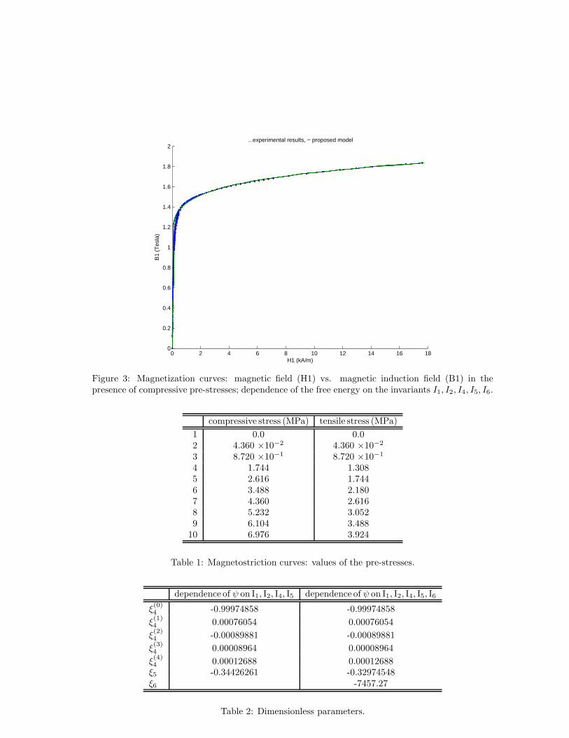
Figure 3: Magnetization curves: magnetic field (H1) vs. magnetic induction field (B1) in thepresence of compressive pre-stresses; dependence of the free energy on the invariants I1, I2, I4, I5, I6.
compressive stress (MPa) tensile stress (MPa)1 0.0 0.02 4.360 ×10⁻² 4.360 ×10⁻²
3 8.720 ×10⁻¹ 8.720 ×10⁻¹
4 1.744 1.3085 2.616 1.7446 3.488 2.1807 4.360 2.6168 5.232 3.0529 6.104 3.488
10 6.976 3.924
Table 1: Magnetostriction curves: values of the pre-stresses.
dependence of ψ on I1, I2, I4, I5 dependence of ψ on I1, I2, I4, I5, I6ξ(0)4 -0.99974858 -0.99974858ξ(1)4 0.00076054 0.00076054ξ(2)4 -0.00089881 -0.00089881ξ(3)4 0.00008964 0.00008964ξ(4)4 0.00012688 0.00012688ξ5 -0.34426261 -0.32974548ξ6 -7457.27
Table 2: Dimensionless parameters.
0 0.2 0.4 0.6 0.8 1 1.2 1.4 1.6 1.8 2−1
0
1
2
3
4
5
6x 10
−6
10
B1 (Tesla)
MS
... experimental results, − proposed model
9
8
7
6
5
4
3
2
1
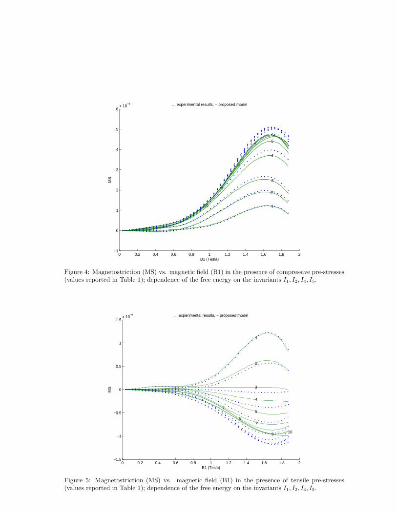
Figure 4: Magnetostriction (MS) vs. magnetic field (B1) in the presence of compressive pre-stresses(values reported in Table 1); dependence of the free energy on the invariants I1, I2, I4, I5.
0 0.2 0.4 0.6 0.8 1 1.2 1.4 1.6 1.8 2−1.5
−1
−0.5
0
0.5
1
1.5x 10
−6
1
B1 (Tesla)
MS
... experimental results, − proposed model
2
3
4
5
6
7
8
9 10
Figure 5: Magnetostriction (MS) vs. magnetic field (B1) in the presence of tensile pre-stresses(values reported in Table 1); dependence of the free energy on the invariants I1, I2, I4, I5.
0 0.2 0.4 0.6 0.8 1 1.2 1.4 1.6 1.8 2−1
0
1
2
3
4
5
6x 10
−6
10
B1 (Tesla)
MS
... experimental results, − proposed model
9
8
7
6
5
4
3
2
1
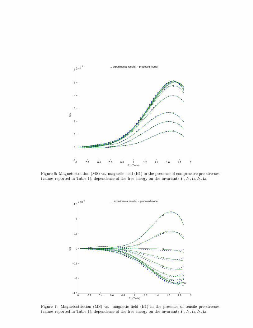
Figure 6: Magnetostriction (MS) vs. magnetic field (B1) in the presence of compressive pre-stresses(values reported in Table 1); dependence of the free energy on the invariants I1, I2, I4, I5, I6.
0 0.2 0.4 0.6 0.8 1 1.2 1.4 1.6 1.8 2−1.5
−1
−0.5
0
0.5
1
1.5x 10
−6
1
B1 (Tesla)
MS
... experimental results, − proposed model
2
3
4
5
6
7
8
9 10
Figure 7: Magnetostriction (MS) vs. magnetic field (B1) in the presence of tensile pre-stresses(values reported in Table 1); dependence of the free energy on the invariants I1, I2, I4, I5, I6.
vacuum are E = 183.62 GPa, ν = 0.34 and µ0 = 4π×10−7 N/A2, respectively. The values of thepre-stresses are reported in Table 1 while Table 2 report the estimated values obtained for thedimensionless parameters.
The results show that the proposed model is suitable to describe the phenomenon of magne-tostriction. It is worth to note that the definition of the coefficient γ4 through the fine polynomialexpansion (17), permitted to correctly describe the effect of the magnetic saturation of the magne-tostrictive strain under high magnetic fields. Furthermore, the dependence of the Helmholtz freeenergy on the invariant I5 is necessary in order to furnish the correct sign of magnetostriction.Finally, the results show that the dependence of the free energy on the invariant I6 is important toaccurately predict the experimental results in the presence of external mechanical pre–stresses. Al-though the proposed model is simple, the obtained results are very good when compared with thoseof the standard square model used in [6] for magnetostrictive materials and based on the expansionin series of the Gibbs free energy. In that paper, the authors had to introduce more complicatedmodels in order to better describe the magnetic saturation at high magnetic fields and the wholephenomenon of magnetostriction even at low values of pre-stresses.
The magnetization curves drawn in Figure 3 for the case of compressive pre-stresses show thatthe results predicted by the theoretical model agree well with the experimental data.
5 CONCLUSIONS
This paper presented a coupled magnetoelastic model for ferromagnetic materials. As proposedby Dorfmann et al. in ([8], [9],[10]), the constitutive equations are written on the basis of theHelmholtz free energy. In particular, the strain tensor and the magnetic induction vector are chosenas the basic variables. A form of the free energy suitable for describing the phenomenon of mag-netostriction in ferromagnetic materials used in electrical machines is presented. The constitutiveequations derived from the proposed free energy depend on the invariants I1, I2, I4, I5 and I6 whichare functions of both the magnetic and the mechanical field. The dimensionless parameters of themodel were evaluated by fitting the experimental data of magnetization and magnetostriction ob-tained by means of a modified Epstein device. The results show a good agreement between themagnetostriction curves obtained from the theoretical model and the experimental results. Sinceboth the magnetic saturation under growing magnetic fields and the magnetostriction in the pres-ence of different mechanical external pre-stresses are described with accuracy, the proposed modelis competitive with respect to the recent magnetoelastic coupled models proposed in literature (see[6]).
Acknowledgments
The present research was funded by TEKES, the National Technology Agency of Finland, in thecontext of the project KOMASI (decision number 40288/05).
REFERENCES
[1] Maugin GA. Continuum Mechanics of Electromagnetic Solids. North–Holland, Amsterdam,1988.
[2] Belahcen A. Magnetoelasticity, Magnetic Forces and Magnetostriction in Electrical Machines.Doctoral Thesis. Helsinki University of Technology, Laboratory of Electromechanics. Report 72(2004).
[3] Besbes M., Ren Z, Razek A. Finite Element Analysis of magneto-Mechanical Coupled Phenom-ena in Magnetostrictive Materials. IEEE Transaction on Magnetics 1996, 32 (3): 1058–1061.
[4] Besbes M, Ren Z, Razek A. A generalized FiniteElment Model of Magnetostriction PhenomenaIEEE Transaction on Magnetics 2001; 37 (5): 3324–3328.
[5] Perez-Aparicio J.L., Sosa H. A continuum three-dimensional, fully coupled, dynamic, non-linear finite element formulation for magnetostrictive materials. Smart Mater. Struct. 2004,13:493–502.
[6] Wan Y, Fang D, Hwang KC. Non–linear constitutive relations for magnetostrictive materials.Int J Engr Mech 2003; 38: 1053–1065.
[7] Fang DN, Feng X, Hwang KC. Study of magnetomechanical non-linear deformation of ferro-magnetic materials. Theory and experiment. Proc. Instn Mech Engrs 2004; 218, Part C: J.Mechanical Engineering Science: 1405–1410.
[8] Brigadnov I.A., Dorfmann A. Mathematical modelling of magneto-sensitive elastomers. Int. J.of Solids and Struct. 2003; 40:4659–4674.
[9] Dorfmann A., Ogden R.J. Magnetoelastic modelling of elastomers Eur. J. of Mech. 2003;22:497–507.
[10] Dorfmann A., Ogden R.W., Saccomandi G. Universal relations for non-linear magnetoelasticsolids. Int. J. Non–Linear Mech. 2004; 39:1699–1708.