Embed Size (px)
Citation preview
Arch. Rational Mech. Anal. 125 (1993) 99-143. �9 Springer-Verlag 1993
Energy Minimizers for Large Ferromagnetic Bodies
ANTONIO DE SIMONE
Communicated by R. D. JAMES
Table of contents
Introduction . . . . . . . . . . . . . . . . . . . . . . . . . . . . . . . 99 1. Micromagnetics: large bodies and small particles . . . . . . . . . . . . . 103 2. Large bodies: asymptotics . . . . . . . . . . . . . . . . . . . . . . . 108 3. Large bodies: energy relaxation . . . . . . . . . . . . . . . . . . . . . 111 4. Large bodies: restrictions on minimizing magnetizations . . . . . . . . . . 121 5. Virgin magnetization curves for large spheres . . . . . . . . . . . . . . . 128 Appendix: magnetostatics . . . . . . . . . . . . . . . . . . . . . . . . . 140 Acknowledgements . . . . . . . . . . . . . . . . . . . . . . . . . . . . 141 References . . . . . . . . . . . . . . . . . . . . . . . . . . . . . . . . 142
Introduction
The problem of predicting the macroscopic response of a permanent magnet to an applied magnetic field from the knowledge of a few constitutive parameters is, in many respects, still unsolved. Magnetization curves, namely, plots of (some measure of) the average magnetization versus the strength of the applied field, give the most basic description of the response of a given specimen. Micromagnetics, a widely used phenomenological model of the behavior of ferromagnetic materials, provides a strategy for the computat ion of magnetization curves. According to micromagnetics, the state of a rigid fer- romagnetic body is described through its magnetization, a vector field defined over the body. Observed magnetizations are assumed to correspond to minimizers of an energy functional E e, which depends on the applied magnetic field. Thus computing magnetization curves amounts to averaging the minimizers of E e, for each value of the applied magnetic field. However, the analytical difficulties involved make this program too hard to implement in cases of practical interest.
The required computations become more manageable if we adopt a simplified formulation o f micromagnetics ("no-exchange" formulation, pro-
100 A. DE SIMONE
posed in [JK90]), obtained by omitting one of the terms of the energy func- tional (the exchange-energy term). In this paper, I show that the no-exchange formulation arises naturally as a limiting case of micromagnetics, the case of large bodies (Sections 1 and 2). I compute the relaxation E** of the no-ex- change functional E (Section 3) and show that, in spite of the non-uniqueness of minimizers of E**, their average is uniquely determined by the applied field (Section 4). Finally, I show that, for a specimen of given shape and increasing size, the average of the absolute minimizers of E ~ tends to the average of the corresponding minimizers of E** (Section 4). In other words, the magneti- zation curves that one would compute from absolute minimizers for micromagnetics tend to those obtained by omitting the exchange energy. That the latter are indeed computable for simple but realistic geometries allows for a comparison between theoretical predictions and measured curves (Section 5). Clearly, this comparison is meaningful only when the measured curves can be thought of as representing absolute minimizers of E c. This is sometimes the case for virgin magnetization curves of defect-free specimens. The good agree- ment of the computed curves with the experimental measurements confirms the reliability of micromagnetics for modelling the macroscopic behavior of ferromagnetic materials.
The focus of this paper is on absolute minimizers. As a consequence, hysteresis is left out of the picture. In the large-body limit, this is immediately clear from the fact that the relationship between applied magnetic field and average of absolute minimizers is one-to-one. In fact, in micromagnetics, hysteresis is associated with the existence of several local minimizers (with dif- ferent averages) under the same applied magnetic field. I plan to address the issues arising in the modelling of hysteresis in a forthcoming paper.
In recent years micromagnetics has attracted the attention of workers in the Calculus of Variations [Vs85, Avgl, JK90, Rogl, Ta92, BR92, JK92, JM92, Pe92] and of numerical analysts [Ma91, LM92]. In particular, the successful application of Young measures in modelling fine phase mixtures in crystalline solids (see [BJ92] and the references quoted therein) has inspired the use of similar tools for modelling the fine domain structures often observed in fer- romagnetic materials. This has led to considering sequences of magnetizations that develop finer and finer spatial oscillations as a mathematical representa- tion of fine magnetic domains (i.e., regions of the body where the magnetiza- tion is approximately constant). Weak limits and Young measures are used to keep track of some of the asymptotic properties of these sequences in the limit of infinite refinement. Loosely speaking, at each point x of the body, the Young measure generated by a sequence of magnetizations [mk} gives the limiting distribution of the values of m k in a vanishingly small neighborhood of x. The weak limit of {ink} characterizes the limit of the average of m k over every subset of the body.
One of the goals of this paper is to clarify the physical meaning of these infinitely refining sequences of magnetizations and to discuss their relevance for applications. I show that they arise naturally in the study of large bodies, by considering a sequence of minimizers of the micromagnetics functional on specimens of given shape and increasing size, and by rescaling them onto a
Large Ferromagnetic Bodies 101
reference body of the same shape and of fixed size. It turns out that a se- quence of rescaled minimizers is a minimizing sequence for the energy func- tional of the no-exchange formulation. Since the no-exchange functional does not penalize interfaces between magnetic domains, this leads, in some cases, to rescaled sequences that exhibit infinite refinement. Essentially, refinement is promoted by the interaction of two terms of the energy functional, namely, the anisotropy energy and the magnetostatic energy. The first forces the magnetization to align with certain preferred directions, the second penalizes magnetizations that are not divergence-free.
An illustrative example of infinite refinement is provided by the power laws that have been proposed (see, e.g., [Hu67]) to express the width of magnetic domains in a thin plate made of a uniaxial material as a function of the plate thickness 2. If the easy axis e is orthogonal to the mid-plane of the plate, and if no external field is applied, then energy minimization leads to domains that are elongated in the direction of e, with magnetization parallel to e and reversing across adjacent domains. For large 2, the width of the domains in the mid-plane of the plate is expected to grow with 2 according to the power law 22/3, while domains at the surfaces of the plate parallel to the mid-plane should tend to a constant width. An isotropic rescaling of these domain pat- terns onto a plate of unit thickness produces infinite refinement.
An interesting feature of the example above, illustrating the limitations of the no-exchange formulation, is the separation of scales of the domain widths at the surfaces and in the center of the plate (see [KM92] for the analysis of a similar branching phenomenon that occurs in a model problem arising from the study of crystalline microstructures). The occurrence of branched patterns has an intuitive explanation. While at the surfaces, domain refinement reduces the magnetostatic energy, there is no advantage for fine structure in the in- terior. On the contrary, exchange energy penalizes domain interfaces, and hence it favors coarser domains in the center of the plate. A branched pattern may result as the compromise between these competing effects (see [Li44, Hu67, Pr76, Hu92]), and it is in fact often observed (see, e.g., [Ch64, p. 228]). Due to the omission of exchange energy, the no-exchange formulation does not allow for an analysis of domain branching. The distinguished feature of se- quences exhibiting branching is that the length scale of the oscillations of the magnetization is not constant throughout the specimen. The no-exchange for- mulation does not discriminate between these sequences (which presumably represent more accurately sequences of micromagnetics minimizers on bodies of increasing size) and those that do not exhibit branching, as long as they have the same limiting energy. A closely related issue is that the Young measure of an oscillating sequence carries no information on the length scale at which oscillations take place. For the prediction of the geometric details of observ- able domain patterns, a selection criterion (in the spirit of [Mti90, Mii92] or of lAB90, AV91]) is needed to choose, among the minimizing sequences of the no-exchange formulation, those "coming from" the full micromagnetics theory.
Rather than pursuing these issues further, I here address the question: What is the no-exchange model good for? The basic answer is that it captures
102 A. DE SIMONE
the asymptotic behavior of some macroscopic quantities of physical relevance, namely, the magnetic field generated by energy-minimizing magnetizations, and their averages over the whole body. Hence, in particular, the no-exchange model is useful for the prediction of magnetization curves for sufficiently large bodies. The key observation is that if {ink} is an arbitrary minimizing se- quence for the no-exchange functional E (under a given applied field), then the sequence of averages [(mg)} converges, and its limit is the same for all minimizing sequences of E (under the same applied field). On the other hand, being a (no-exchange) minimizing sequence is much less stringent a require- ment than being a sequence of rescaled minimizers of the full micromagnetics functional for bodies of increasing size. It is precisely the "degeneracy" of the large-body-limit problem that proves expedient to compute more easily some limit properties of the solutions of the micromagnetics problem.
The actual computation of magnetization curves is based on computing minimizers of the relaxation E** of the no-exchange functional E. This can be formally defined as
E**(m) := inf IlikrninfE(mk) :mk~ m I ,
where ~ denotes weak convergence. In other words, E** (m) gives the lowest energy attainable by a sequence whose asymptotic macroscopic representation is m. Thus E** represents a macroscopic or effective energy of the system. I give a formula for E** and show that the infimum of E** is always attained and that minimizers of E** are always weak limits of weakly converging minimizing sequences of E. For these sequences, the limit average magnetiza- tion is well defined, and it is just the average of the weak limit. Thus the large- body-limit magnetization curves can be obtained by computing, for each value of the applied magnetic field, the average of any one of the minimizers of E**. A similar analysis can be performed in terms of Young measures rather than weak limits. This would lead to the definition of
EYM(Vx):=infIlikm~fE(mk):m k generates the Young measure vx l ,
as the effective energy of the system. Since Young measures give a more de- tailed description of the asymptotic behavior of a sequence, this formulation provides a deeper insight on minimizing sequences of E. However, the com- putation of minimizers of E** represents a natural first step in the computa- tion of minimizers of E TM. Moreover, a careful analysis of the structure of E reveals that the Young measures of minimizing sequences of E (equivalently, the minimizers of E TM) can be reconstructed from the knowledge of the minimizers of E** (see Proposition 4.7).
The results of this paper shed light on the method currently employed by material scientists to compute virgin magnetization curves of defect-free specimens. Due to the difficulties encountered in trying to apply micromagnetics directly, a simplified model, called phase theory in [Hu92],
Large Ferromagnetic Bodies 103
has been devised to perform the task. Phase theory dates back to the work of N~EL [N644] and LAWTON & STEWART [LS48]. The observation that a magnetic domain can be thought of as a region in which a single magnetic phase (i.e., magnetization vector) is present explains the name of the theory. In the conven- tional view, phase theory is derived from domain theory (see [JK90] or [BR92] for a brief account) by simplifying the expression for the energy. The energy associated with domain interfaces is neglected (this is considered acceptable for large specimens) and the magnetostatic energy is computed by substituting the actual magnetization with its average (this is considered acceptable for ellipsoidal specimens). This leads to an approximate effective energy, E PT which is deter- mined by the knowledge of the phases present in the specimen, and of the volume that they occupy. Magnetization curves are computed in the obvious way, via energy minimization. The method has been successfully applied to the prediction of magnetization curves for ellipsoidal samples under a spatially constant magnetic field.
A deeper understanding of the reasons for the success of phase theory can be achieved by a comparison with the methods described in this paper. In fact, the energy E er used in phase theory is a special case of the E** that I com- pute by relaxation. Moreover, E TM represents the Young measure version of phase theory; it is related to large-body micromagnetics in exactly the way Young measure versions of mixture theory (see [BK90]) are related to the ther- mostatics of fluids. For ellipsoids, one can find minimizers of E** or of E TM
that are spatially constant and, for these, the energies E er, E**, and E TM
coincide. Thus one can conclude that, for ellipsoidal specimens, phase theory computes correctly the large-body-limit magnetization curves corresponding to absolute minimizers of micromagnetics. In addition, my derivation of phase theory from micromagnetics shows the form of phase theory that one should use for arbitrary specimen geometries and applied fields.. This may be of significant help in setting up reliable numerical computations of magnetization curves for realistic specimen geometries.
As a final introductory remark, I acknowledge my debt to the sources that provided the motivation for the work reported on this paper. Many of the ideas discussed here are already present in, or directly inspired by [JK90]. The possibility of generalizing results and methods of [JK90] was suggested to me by the computations reported in Section 5, and confirmed by results of TARTAR [Tagl], which appeared in [Ta92]. Finally, the remarkable reliability of the predictions of phase theory, of which I was aware from textbook discussions (see [Ch64, Zi67]), motivated my attempts at a deeper understanding of its methods. The basic tool I used for this purpose is weak convergence. For background material on weak convergence and on the direct methods of the Calculus of Variations, the reader is referred to [Bz87] and to IDa89].
1. Micromagnetics: large bodies and small particles
Micromagnetics, a continuum model of the macroscopic behavior of a body of ferromagnetic material, emerged as a consistent theory from a set of
104 A. DE SIMONE
scattered investigations (among which [LL351 stands as a classic of paramount importance) with the work of BROWN (see [Br63] for a detailed account of the theory and of its historical background). Throughout this paper I restrict my attention to the case of a rigid, homogeneous body, identified with the region of space 2 that it occupies, which I assume to be an open, bounded, connected subset of ~3 with Lipschitz boundary. Under these assumptions, the fundamental quantity describing the state of a ferromagnetic body is a vec- tor field, the magnetization m, defined on ~ . The magnetization field represents a volume density of macroscopic magnetic moment, and this means that m induces a magnetic field hm at all points of space (see the Appendix for the definition and the relevant properties of hm). An important assump- tion of the theory is that a ferromagnetic body is always locally saturated, namely,
Ira(x) I = m~ > 0 in ~_~, (1.t)
so that a specimen can achieve a demagnetized state only in an average sense. The scalar ms, called saturation magnetization, is, for a given material, a func- tion of temperature only. Since I assume that the specimen at hand is at a fixed temperature falling in the range in which the material exhibits fer- romagnetic behavior, ms can be regarded as a material constant.
According to micromagnetics, the observable states of a ferromagnetic body subject to a given external magnetic field he can be modelled as absolute (or possibly relative) minimizers of the energy functional
E~e(m,~.~ ) =�89 2 .[IVml 2 + ~o(m)- Ihe .m+�89 ~Ihm[ 2 ~Y 3 ~3
(1.2)
Each of the summands in (1.2), called respectively exchange energy, anisotropy energy, interaction energy and magnetostatic energy, can be regarded as a penalty term that enforces a certain feature of the observed behavior of fer- romagnets. The exchange-energy term, in which o~ 2 is a positive material con- stant, models the tendency of a specimen to exhibit large regions of uniform magnetization (magnetic domains) separated by very thin transition layers (domain walls), by penalizing spatial variations of m. Expressions for the anisotropy energy density more general than that used here are possible. All the results of this paper are still valid if one replaces ~21Vm[2 in (1.2) by Vm. A Vm, where A is a positive-definite 3 x 3 matrix. The anisotropy energy, in which (p is a non-negative, even function exhibiting crystallographic sym- metry, models the existence of preferred directions of magnetization (easy axes), along which ~0 is assumed to vanish. These axes manifest themselves as the directions of a spatially constant external magnetic field under which a specimen achieves uniform magnetization (saturation) at smallest field strengths. I assume that (p is the restriction to ms $2 := {xE [R 3 : I X [ = ms} of a non-negative, even function 0 6 C = (N3). In fact, fp is usually taken to be a polynomial in m. The interaction energy models the tendency of a specimen to have its magnetization aligned with the external field he, assumed to be unaffected by variations of m. I also assume that he EL2oc(R 3, JR3). Finally,
Large Ferromagnetic Bodies I05
the magnetostatic energy is the energy associated with the magnetic field generated by m, and it is minimized by divergence-flee magnetization fields. Its expression can be justified via atomic lattice calculations (see [Br62] and [JM92]).
As remarked in the Introduction, in this paper I restrict my attention to absolute minimizers of the energy functional (briefly minimizers in what follows), namely, to solutions of the problem:
Minimize E~,(m, ~ ) amongst functions m EHI(~,msS2), (1.3)
where Hl(~.~,ms $2) := {v(Hl(~, [R 3) :lvl = ms a.e. in ~} is the set of vec- tor fields for which (1.2) is finite. Using the direct methods of the Calculus of Variations, VISINTTN [Vs85] has shown that (1.3) admits at least one solution for every he, but the actual computation of solutions in cases of practical in- terest is far from trivial. However, at least in the limit cases in which ~ is either very large or very small, the minimization problem (1.3) can be somewhat simplifed because the exchange energy and the remaining terms in (1.2) scale differently with respect to the body size.
Magnetization fields observed in ferromagnetic bodies of a given shape, but of different sizes, can vary dramatically. For example, very small spheres tend to be uniformly magnetized, while sufficiently large ones can exhibit fine domain structures. To understand how the energy terms in (1.2) are affected by volume rescalings, consider a ferromagnetic body 2 of volume 23, where 2E (0, ~) , and let ma~Hl(~,ms $2) and he~L2oc(R 3, [R 3) be given. Set f2:= ( 1 / 2 ) 2 and define m:f~msS 2 and h : R 3 ~ R 3 by
m ( 2 z ) :=ma(z ) , z~J2,
h ( l z ) :=he(z), z~ [R 3.
Clearly f2 is an open, bounded, and connected set having a Lipschitz bound- ary and unit volume. Moreover, mEH~(f2, msS 2) and hfL2oc(~3,~3). It is also useful to note that in the particular case of a constant he, which is the most natural and interesting for applications, h = h e. Denoting by ha and hm the magnetic field generated by m a and m, and using the uniqueness of the solution of (A.2), we easily show that
h m ( l z ) = hz(z), Z E [ ~ 3 ,
and hence
1 E~e (m'~' ~'~) = E~/a(m' f2)
= 2 ~ l V m l 2 + o ( m ) - h . m +�89 [hm[ 2. (1.4)
Rs
106 A. DE SI~ONE
Since, for given he, the field mx is an energy minimizer for ~2 if and only if it minimizes (1.4), one can study the effect of variations of the size of the specimen by studying the minimizers for the reference body ~ under the scaled external field h, and varying the exchange constant. In particular, (1.4) natural- ly suggests two limit problems, as the scale parameter ,~ approaches the ends of its range~.
(a) Small particles: 2 ~ 0
As 1/)L 2 becomes large, the exchange energy becomes the dominant term in (4). This suggests that one consider the problem
~_@~': Minimize
Eh(m) '= l i b ( m ) - h . m } + � 8 9 2
amongst constant functions m : ~-+ ~3 such that [m I = in ~.
It is easy to show (see [De92]) that ~ =always has at least one solution, and that solutions of ~ oo capture the limit behavior of minimizers of the energy functional of micromagnetics in the following sense. For a given h, let mk be a minimizer of (1.4) corresponding to )L = l/k, k 6 N, and let moo be a solu- tion of ~oo . Then (i) Eh(mk) ~Eh(moo) as k--, oo. (ii) There exists a subsequence of [mk} that converges strongly in Hi(f2, ~3)
to a solution of 3oo . In particular, if moo is the unique solution of ~@oo, then mk~moo in Hl(f~, R3).
Problem ~@oo was posed by S x o ~ R & WOHLF~TI-I in [SW48] for a body of ellipsoidal shape under a constant magnetic field. This case is of special interest since, for an ellipsoid under a constant applied field, con- stant magnetizations satisfy the Euler-Lagrange equations associated with (1.3), and solutions of ~ ~ represent the actual micromagnetics minimizers for a non-empty range (O, Xc(h)) of the scale parameter. For ,~ < 2 c ( h ) , f~ is said to exhibit "single-domain" behavior, and explicit bounds on )L c have been computed for the case h = 0 (see [Br691 for bounds on the critical radius Rc = (3/4rc)l/3)Lc below which a spherical specimen exhibits single-domain behavior and [Ah88] for similar calcula- tions for ellipsoids).
1 The idea used here is essentially the same as that used in the study of the equilibrium shape of liquid crystal drops, e.g., in [Vr89].
Large Ferromagnetic Bodies 107
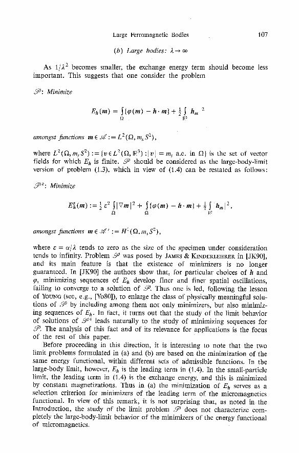
( b ) Large bodies: ~ ~ oo
As 1/)L 2 becomes smaller, the exchange energy term should become less important. This suggests that one consider the problem
~ : Minimize
Eh(m) = ~(~o(m) - h . m } + �89 ~]hml 2 R 3
amongst functions m ~ S : = L 2 (if], m s $2),
where L 2 ( ~ , m s $2) := {vEL2(f2, R 3) :lvl : ms a.e. in f~} is the set of vector fields for which Eh is finite. ~ should be considered as the large-body-limit version of problem (1.3), which in view of (1.4) can be restated as follows:
3 e: Minimize
E~(m):=�89 2 jlVml2+ ~[q~(m) - h . m } + �89 jlhzl 2, ~ ~3
amongst functions m ~ d ' := Hi(f2, m s $2),
where e = o~/2 tends to zero as the size of the specimen under consideration tends to infinity. Problem ~ was posed by JAMES & KINDEgL~I-Im~R in [JK90], and its main feature is that the existence of minimizers is no longer guaranteed. In [JK90] the authors show that, for particular choices of h and (p, minimizing sequences of Eh develop finer and finer spatial oscillations, failing to converge to a solution of ~ . Thus one is led, following the lesson of YOVNG (see, e.g., [Yo80]), to enlarge the class of physically meaningful solu- tions of ~ by including among them not only minimizers, but also minimiz- ing sequences of Eh. In fact, it turns out that the study of the limit behavior of solutions of ~ e leads naturally to the study of minimizing sequences for ~@. The analysis of this fact and of its relevance for applications is the focus of the rest of this paper.
Before proceeding in this direction, it is interesting to note that the two limit problems formulated in (a) and (b) are based on the minimization of the same energy functional, within different sets of admissible functions. In the large-body limit, however, Eh is the leading term in (1.4). In the small-particle limit, the leading term in (1.4) is the exchange energy, and this is minimized by constant magnetizations. Thus in (a) the minimization of Eh serves as a selection criterion for minimizers of the leading term of the micromagnetics functional. In view of this remark, it is not surprising that, as noted in the Introduction, the study of the limit problem ~ does not characterize com- pletely the large-body-limit behavior of the minimizers of the energy functional of micromagnetics.
108 A. DE SIMON~
2. Large bodies: asymptoties
The scaling argument that leads to considering the no-exchange formula- tion as a large-body-limit version of micromagnetics is, at this stage, merely heuristic. It is then natural to ask in which sense the generalized solutions of the limit problem ~@ (i.e., minimizers and minimizing sequences of Eh) repre- sent the limit behavior of solutions of problem ~,o=, as e-->0. The main result in this direction is Theorem 2.4. Loosely speaking, it asserts that sequences of minimizers of E~, are minimizing sequences for Eh. In fact, a similar result can be expected to hold in more general situations. As the following easy prop- osition shows, the key point is that there is no gap between the infimum of Eh in S and the infimum of Eh in the smaller set d ' (recall that S ' and d are respectively the sets of vector fields with finite energy in the full theory and in the large-body-limit theory).
Proposition 2.1. Let E : S ~ ~ and D : S ' ~ [0, oo) be two given functionaIs, with S ' C S . For every e > O, let E s : = eD + E : d ' ~ R and assume that there ex- ists m e s 5 J ' that minimizes E e in d ' . Then the following propositions are equivalent: (i) l i m E ( m e ) = in fE ,
e--+O
(ii) i n fE = infE. (2.1)
Proof. (i) = (ii) is obvious. To show the opposite implication, observe that m e ~ S ' C S . Thus
l iminfE(me) ____ in fE . (2.2) e ~ 0 ~r
But since D >_ 0 and m e is a minimizer of E e, it follows that for every m s
E(mE) <= Es (ms) <-_ e D ( m ) + E ( m ) .
Thus
and, by (2.1),
l i m s u p E ( m = ) <= E ( m ) , e~O
lim supE(ms) < in fE = in fE . (2.3)
Hence (i) follows from (2.2), (2.3) and the fact that l iminf =< lira sup. []
In fact, the "no-gap" condition (2.1) holds for the case of micromagnetics (with E h replacing E). This is shown in Lemma 2.3. In its proof I make use of the following approximation result, which I state separately for later reference.
Large Ferromagnetic Bodies 109
Proposition 2.2. For every
m ( d * : = [ v 6 L 2 ( ~ , N 3 ) : l v ] <_m~ a.e. in f21,
there exists a sequence {n~} C S * of piecewise constant functions such that n k ~ m in L2(~, ~3) as k---> oo.
Proof. This is a standard result. Here it is proved for a specific class of piecewise constant approximants of a function in S * D 54'. Let m ~ H * be given and let [el,e2, e3} be a set of orthonormal vectors in ~3. For every k ~ N consider the cubic lattice
el, Y 1, V 2, E ~ , Lk:= x ~ R S : x = ~ ~ v i v 3
i=1
having as unit cell the cube
U k : : X ( ~ 3 : X : 2k o~iei, O~o~i~ . 1, i = 1,2,3 i=l
of edge length 2 -k. Since ~ is bounded, there exist N ( k ) ~ ~q and a finite collection of N(k) non-empty disjoint subsets of f2 of the form f2kj = f2 n {Xj + U~}, with xj ~ Lk and j = 1 . . . . . N(k) , such that
N(k) I,J f2ky = f~. (2.4)
j= l
For every k ~ N, the piecewise constant vector field defined by
nk(y) := ? 3 ~ j m ( x ) d x yEf2~j, j = 1 . . . . ,N (k )
is in d * , and (see [JM92, Proposition4.1]) n k ~ m in L2(~'2,[~ 3) k ~ w . []
(2.5)
Lemma 2.3. For every h EL2oc([R 3, jR3),
Proof. Since d ' C sd,
as
~,fEh = infEh. (2.6)
To prove the reverse inequality, I prove the following two assertions.
Assertion 1. For every m ~ d , m k ~ m in L2(~ , •3).
there exists a sequence {mk} C S ' such that
110 A. DE SIMONE
Proof of Assertion 1. Let nk be as in (2.5). Note that for every k, n k has finite range (i.e., it takes on only finitely many values) and nk~m in L2(g), R3). Set
(nk(x) ~lnAx) lms if nk(x) * O,
~k(X) / ".urns if n~(x) = O,
where u is an arbitrary fixed unit vector, and note that, in view of the iden- tities
]ak(x)- nk(x)l =lms-ln~(x)ll = IIm(x)[- [~(x)ll a.e. in f2,
r i ~ r n in La(f2, [R 3) by the triangle inequality and the fact that n~--,m. I now show that each of the ~ can be approximated in La(f2, ~3) by a sequence of elements of S ' . Fix k, and let g := ~k. The function g: R3--,m~S 2 defined by
( g ( x ) for x ~ ~ , g(x)
l kUms for x~ ~ 3 \ f 2
has finite range. Hence there exists z~rnsS 2 and a closed ball B(e,z) of radius e centered at z such that range (g) c3 B(e, z) = 0. Thus the stereographic projection n z, with projection center z, maps range (g) into a bounded subset of [R 2. Denoting by {Pl/n} C Co~ (JR 3) a sequence of mollifiers, one has
gn : : 7"gz 1 o LOl/n �9 (TZzog)] E C I ( R 3, jR3),
where n z ~ is the inverse of n z, o denotes composition and * denotes convolu- tion. Moreover, [gn[ = rn~ in R 3 and gn~g in L~o~(FR s, FR3). Letting g~ be the restriction of g~ to f~, one obtains a sequence {g~} C S ' such that gn~g in Le(f2, FR s) as n ~ oo.
Repeating this procedure for each of the ~k, one can define sequences [gk,~}~N of elements of S ' such that gk,~r~g in L2(f2, rR 3) as n ~ o o . Choosing for every k an index n(k) such that the L 2 norm of (gk,~(k~ -- r~g) is less than 1/k and letting mk:= gk, n(k~ concludes the proof of Assertion 1. []
Assertion 2. inf, Eh < i n f E h �9
Proof of Assertion 2. Let {nk} C d be a minimizing sequence for Eh. For fixed k, I use Assertion i to approximate nk with a sequence in S ' that con- verges strongly in L2(f2, VR 3) to n~. Since the magnetostatic energy is con- tinuous in the strong topology of L2(f), [R 3) (see (A.4)) and since ~o is con- tinuous on the compact set ms $2, E h is continuous in the strong topology of L2(~ , ~3). Thus for every k~ •, there exists rake S ' such that Eh(mk) <
Large Ferromagnetic Bodies 111
Eh(nk) + 1/k. Therefore
infEhg, =< g-~liminfEh(m~) =< inf Eh. []
Having shown that (2.1) holds with Eh in place of E, one can read off the following theorem 2 from Proposition 2.1.
Theorem 2.4. For every e ~ O, let me E S ' be a minimizer of E~. Then
e-~olim Eh (me) = inf Eh .
3. Large bodies: energy relaxation
I turn now to the study of minimizing sequences of Eh. As already men- tioned, the infimum of Eh in d may be unattainable by elements of S , and minimizing sequences may develop increasingly finer spatial oscillations. However, due to the constraint (1.1) and to the fact that ~ is bounded, se- quences of magnetizations are always bounded in L2(~, R3); hence they ad- mit weakly convergent subsequences. In view of Theorem 2.4, it is of great in- terest to try to characterize the subsequential weak limits of minimizing se- quences of Eh (i.e., the limits of weakly convergent subsequences extracted from minimizing sequences of Eh). For this purpose, following E~ZEtAND & TEMAM [ET76, page 389], one may try to find a relaxed version of problem ~@, based on the minimization of a new energy functional E~,* (the relaxation of Eh) whose infimum is attained at the value infEh and having the property that its minimizers are precisely the subsequential weak limits of the minimiz- ing sequences of Eh. In this section, I show that this relaxed problem can be formulated as
~@* : Minimize
E~,*(m):= ~ { ( o * * ( m ) - h . m } + � 8 9 ~lhml 2 f] ~3
amongst functions m~ d * = [vELe(f~, [R s) :Iv I __< ms a.e. in f2},
where ~0"* is defined by
~0**(y): = s u p ( f ( y ) : f : ~ 3 - - , ~ is convex and f__<~0 o n rosS2}, Y E~3, [Yl <=ms.
The function r the convexification of ~o, can be alternatively characterized as follows (see, e.g., [Da89]):
(o**(y) = i n f ~.i(P(Yi) : ~.iYi = Y , hi >: O, ~-i : l , y i E m s $2 , i=1 i=l i=1 (3.1)
and some of its properties are collected in the next proposition.
2 A partial result in this direction is in [Ma91].
112 A. DE SIMONE
Proposition 3.1. Let msB := {y fi R 3 :[y[ < ms}. Then (i) The infimum in (3.1) is attained for every y ~ msB. (ii) For every y E ms S 2, (o** (y) = (o (y). (iii) (o** is convex on msB. (iv) (p** is in C i on ms B.
(3.2)
Sketch of the Proof. Proposition (i) follows from the fact that the function f: [0, 114• (msS2)4~R, defined by
4
f ( 2 1 . . . . . 24;Yl . . . . . Y4) : = ~ 2ir i=1
is continuous on the compact set
(21 . . . . . 24;Yl . . . . , Y 4 ) S [0, 114X ( m s S 2 ) 4 : 2 i = ] , 2 i y i = y .
i=1 i=1
Proposition (ii) reflects the fact that a point of ms S 2 can be expressed as a convex combination of points of ms S 2 only in a trivial way. Proposition (iii) is standard, since (0"* is the pointwise supremum of a family of functions that are convex and finite in msB. Also the continuity of q~** in (msB) ~ the in- terior of msB, is standard, and the continuity up to the boundary is a simple consequence of the strict convexity of msB and of the continuity of (0 on ms $2. However, the proof of the continuous differentiability of (0"* up to the boundary is more delicate. First, observe that, at each point of (msB) ~ the subdifferential of q~** is a singleton. (For, if at some point y in (msB) ~ the subdifferential of r consisted of at least two distinct vectors, then one could construct a piecewise affine, convex fuction ~" such that /_< (0 on msS 2 and / = (0"* at y and at some point x e msS 2 where a tangential derivative of / along ms $2 is discontinuous. Since / i s convex and /_< q) on rosS 2, this would force q~ to have a discontinuity in a tangential derivative, against the assump- tion (0 ~ Ca(rosS2)). Then, by standard results of Convex Analysis (see, e.g., [Rk70]), (o**E C 1 ( (msB)~ Observe now that , since (p** is convex, for every x ~ ms S 2 and unit vector u ~ R 3 such that u . x < 0, the one-sided directional derivatives Du(o**(x) are well defined as limits of Du(o**(x+ ru) , r ~ 0. Moreover, these limits are finite. (Since ~ C~ there exists a convex function g/6 C~~ such that q / = (0 on msS 2 and ~ __< (0"* on msB. Hence (o**(x + ru) - (o**(x ) >= - r M , where M : = m a x { l D ~ / ( x ) ] : x e m s S 2} and D~,(x) is the derivative of ~u at x. Furthermore, by the convexity of cp**, Dufo**(x + ru) => - M . Since D,r + ru) decreases as r ~ 0, it has a bounded limit). For unit vectors te R 3 such that t . x = 0, one can use the last result, the definition of (0"* and the smoothness of q~ to show that, as r "~ O, Dt(o**(x + ru) --*Dt(o**(x) = Dt(o(x), the derivative of (0 along t. The continuity of the directional derivatives leads, via the mean value theorem, to the (continuous) differentiability of (r up to ms $2. []
The continuity of (0"* on ms B has some important consequences. First, in view of (A.4), it implies that E~* is continuous in the strong topology of
Large Ferromagnetic Bodies 113
L2(f2, ~3). Moreover, it implies that E~* is weakly lower semicontinuous. This fact is shown and exploited in the following proposition.
P r o p o s i t i o n 3.2. (Existence of solutions of ~* ) . For every h~L~oc(R 3, [~3), there exists m ~ ~ * such that
E~* (m) = infEr*. X *
Proof. The proof is an easy application of the direct method of the Calculus of Variations. Let [ink} C S * be a minimizing sequence for E~*. Since ]m~l - ms and ~ is bounded, one can extract a subsequence {rn/~} of {ink} that converges weakly in L2(f~, R 3) to, say, m ~ d * . Since ~o** is continuous on the compact set m~B, the functional defined by
m ~ ~ ~o** (m) f~
is continuous in the strong topology of L2(~, ~3) and hence, being convex, it is also weakly lower semicontinuous (see [Da89], Section 3.1.2). But also the other summands of E~* are weakly lower semicontinuous (see (A.5) for the magnetostatic energy term). Therefore
E~*(m) <= u-,~lim a~{(~ ( m Y ) - h ' m v } + ~ Ihm"12 = ~ f E~*'
i.e., m is a minimizer for E~,*. []
The analysis of the relationship between minimizers of E~* and minimiz- ing sequences for Eh, relies on the following approximation result. In its proof I repeatedly use the well-known fact that if f ~ f in L2(f~, ~3) and g k ~ g in Lz(~, R3), then
~fk" gk ~ ~f'g. f2 f~
P r o p o s i t i o n 3.3. For every m ~ S* , there exists a sequence {m~} C S such that, as k ~ oo,
m k ~ m inL2(f2, N3), Eh(mk)~E~*(m ).
Proof. Let m ~ S * be given, and let nk be as in (2.5). Recall that {nkl C sr and that n k ~ m in Le(f~, N3) as k ~ c~. Thus, by the continuity of E~'*,
E~'* (rid ~E~* (m). (3.3)
The rest of the proof is divided into two steps. First, I use a "layers- within-layers" construction to show that each n k can be approximated by a sequence of magnetizations {mk, u}ueN C S such that mk, u ~ nk in Le(f2, R 3) and Eh(mk, , )~E~*(nk) as u~co . The key ingredients in this step are the careful choice of the values of rn~,, in each layer to guarantee the con-
114 A. DE SLUONE
vergence of the anisotropy part of the energy functional, and the careful choice of the layering directions 3, to control the divergence of ink, . , hence ensuring the convergence of the magnetostatic energy of Ink,~ to the magnetostatic energy of nk. Then, using the fact that nk-"In, I show that, for every k, one can choose u = u(k) such that the sequence {ink}keN : = {Ink, u(k)}k~N has the desired properties.
Step 1 : Construction of {Ink, u} C S such that, for each fixed k ~ N, mk, u ~ nk in L2(f~, N3) and Eh(m~:,u)--*E~* (nk). In this construction, k is fixed. Recall that nk is constant in each of the sets Okj partitioning f2. Choose j f i [1 . . . . . N(k)} and, to simplify the notation, set E : = f2kj and let n be the value of nk in E. By construction, ln l ____ ms. Then, by Proposition 3.1, there exist 21 . . . . , 2 4 E [0, 1], with Z2i = 1, and In1 . . . . ,m4Ems $2 such that
4 4
gl = E 2iini' qg**(T t )= E 2i(fl(ini) i=1 i=1
where one can assume, without loss of generality, that 2i =r 0 for i = 1 . . . . . 4. Let
21 22 v : = 2 1 + 2 4 ' ] / 1 " - - 2 1 + 2 4 ' ]/2:-- 2 2 + 2 3 ,
and note that v , ] / 1 , ] /2 E (0 , 1) and
v]/1 = 2 1 , v(1 --/ ' /1) = 2 4 , (1 - v)]/z = 22,
Moreover, let q, Pl, P2 be unit vectors in R 3 such that
{[]/ lnll "q- (1 -- ]/1) me] -- []/2m2 + (1 - ]/2) m311" q = 0,
(ml - m4) "Pl = O, ( m 2 - roB)"P2 = O,
and let O, rh, ~/2 be the l-periodic functions defined by
O(t) := f + l for t 6 [ O , v ) ,
I. - 1 for t~ [v, 1),
rh(t ) := f +1 for t~ [0,]/i),
t~ - 1 for tE ~i, 1),
(1 -- Y) ( l -- ] /2) = 23 . (3 .4 )
i = 1 , 2 .
(3.5)
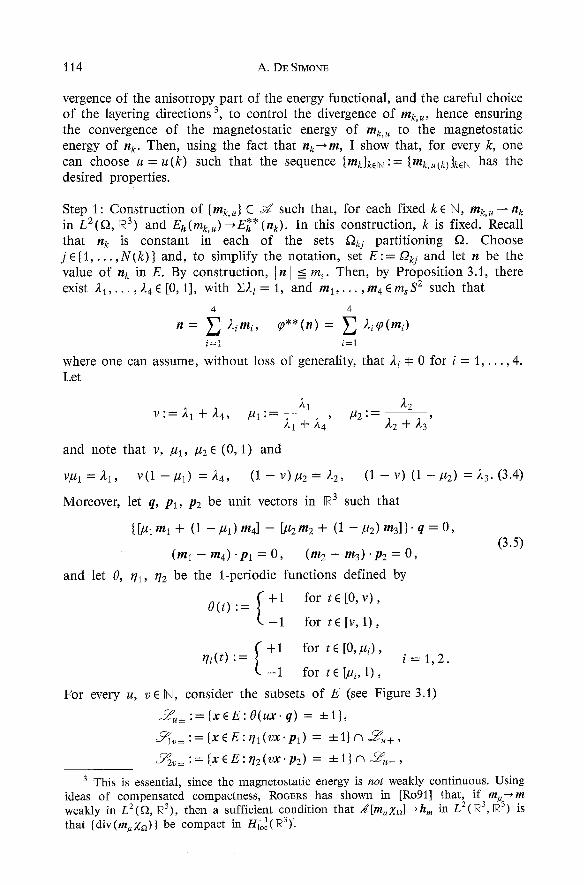
For every u, v~ N, consider the subsets of E (see Figure 3.1)
2 u . ~ : = { x ~ E : O ( u x . q ) = +1},
~-~lv• := [x ~ E: r h (vx. Pl) = -4-1} n 2 u + ,
~ 2 v • = -4-1}n ~ u - ,
3 This is essential, since the magnetostatic energy is not weakly continuous. Using ideas of compensated compactness, ROGERS has shown in [Ro91] that, if mu--*rn weakly in LZ(f2, Rz), then a sufficient condition that ..([mgz~]---~hm in L2(R 3, R 3) is that {div(rnuxa)} be compact in H1~(~3).
Large Ferromagnetic Bodies 115
/ /
-k 2
_ _ _ ~ = 01
\
f2
(a)
]J
1-k~ 2 v
(b) (c)
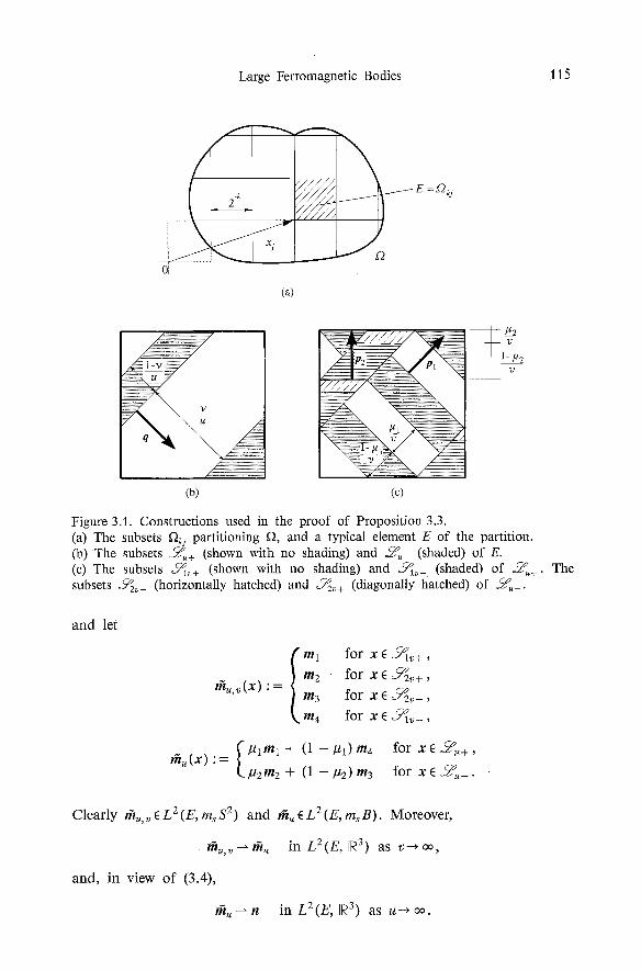
Figure 3.1. Constructions used in the proof of Proposition 3.3. (a) The subsets ~kj partitioning ~, and a typical element E of the partition. (b) The subsets ~ + (shown with no shading) and 2 , (shaded) of E. (c) The subsets ~ + (shown with no shading) and ~ _ (shaded) of 2~+. The subsets ~2~- (horizontally hatched) and ~ + (diagonally hatched) of 2 , _ .
and let
r~,v (x):=
I m I for x E S~lv+,
m 2 for x E ~z~+,
m 3 for x ~ ~ _ ,
m 4 for x ( S~l~-,
f /~ lml -t- (1 - / / 1 )m4 for x ( ~ , + , ~ ( x )
~-/~2 m2 + (1 - / z 2) m3 for x ~ 2 ~ _ .
Clearly rku, ~ ~ L 2 (E , ms S 2) and r~ ~ L 2 (E, ms B). Moreover,
rhu,~ ~ r~. in L2(E, ~3) as v--. ~ ,
and, in view of (3.4),
rku ~ n in L2(E, ~3) as u ~ ~ .
116 A. DE SIMONE
f ar
I a" E
m 4
m u
f(~9(rrtu,~,(~,,v)fQ9 ( l l )
E E
nu,v n u
A~ [nu,v XE] ~ 0
n u = / n u - - /'/
~( [nuXe] ~ 0
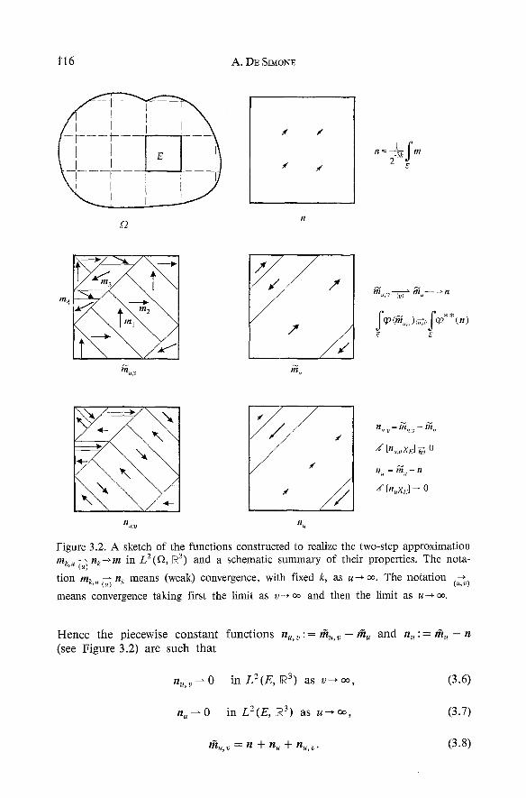
Figure 3.2. A sketch of the functions constructed to realize the two-step approximation mk,~ ~ n k ~ m in Lz(f2, [R 3) and a schematic summary of their properties. The nota-
tion ink,. ~.~ nk means (weak) convergence, with fixed k, as u ~ co. The notation (u,v) means convergence taking first the limit as v--, co and then the limit as u-~ co.
Hence the piecewise cons tant funct ions nu, v : = t h~ ,~ - th~ and n . : = t h . - n (see Figure 3.2) are such that
nu, v ~ 0 in L 2 ( E , ~3) as v ~ oo, (3.6)
n u ~ 0 in L Z ( E , N3) as u---~ oo, (3.7)
rku, v = n + nu + nu, v. (3.8)
Large Ferromagnetic Bodies 117
Furthermore,
X E ~ l v + ~ nu, v(X) = m l - - f l lm l -- (1 -- i l l ) m 4 = (1 - g l ) ( m l -- m 4 ) ,
and therefore, by (3.5)2,
n~,v(X).pl = 0 in ~lv+. Similarly,
rtu, v(X) 'Pl = 0 in S~v_, n,,v(x).pz = 0 in ~ v •
n~(x).q=O in 2 , •
Thus if ~u,v ~ H 1 (~3) is such that V%v = - A'[n~,vXE], then by (A.6) and the divergence theorem,
~ I , r 12 = - ~ n~ .~zE, x[,,~.vz~] = S ,,~.vz~. v~uv ~3 ~3 Rs
= ~ ~u, vnu, v" v+ + ~ ~u, vllu, v " v - , 02.+ a~_
where v+ and v_ are respectively the outer unit normals to a ~ + and a2~_. But, for fixed u, (3.6) and the weak continuity of ~ imply that V#,,v~ 0 in L2(~ 3, [R 3) as v~c~. Hence by the Rellich theorem and trace theorems, u~,v~0 in L2(O~u+) and in L2(O~u_), and since Inu, vl is uniformly bounded,
A'[nu, vZe] ~ 0 in L2( [R 3, R 3) as v~oo. (3.9)
A similar argument based on (3.7) shows that
A'[nuxE]-~0 in L2(~ 3, ~3) as u--. c~. (3.10)
By (3.8) and (A.6), exploiting the linearity of ~, and using (3.6) and (3.9), (3.7) and (3.10), one gets
lim f lim ~l '~[r~,v Ze]]21
fl,m [- U ---~ o o ~ V ---> Co
= lim f - (
I (l't'b nu-.]-nu, v). /~[ (n-]-nu-[-nu, v))~E]II E
(n + nu). A'[(n + n.) ZE]I E
= ~ I ~[nxE] 12. R3
Hence for every uE N, one can choose v(u)~ N such that, as u--,co,
A'[th,,v(,) Ze] --'/Z[nze] in L2([~ 3, /~3). (3.11)
118 A. D~ SIMONE
By construction, on every cube D C E, th,,v(,) takes on precisely the four values in I . . . . . m 4 on disjoint sets covering D whose measures tend to ~,11D [ , . . . , ~4[ D [. Thus, by a standard characterization of weak convergence (see [Da891), it follows that, as u~oo,
rk~,v(u) XE ~ nze in L2([~ 3, ~3) , (3.12)
S S 4 S (O(rku, v(u))~ E ~'i(P(mi) = (,0**(rt). (3.13) i=1
E E E
Since E = f~kj is an arbitrary element of the partition of f~ shown in Figure 3.1(a), the same construction can be repeated for each of the r Thus, for every fixed k~ N, the sequence {mk,~}~N defined by
rnk,.(x) := thu, v( . ) (x) , x ~ f2kj, j = 1 . . . . . N ( k ) , (3.14)
is such that mk, u~nK in L2(f2, N 3) and Eh(mk, . )~E~*(nk) , as u--. c~. The only non-trivial step in the verification of this fact is checking that ~r ,([nkXa] in L2(~ 3, R 3) as u-+ ce. This follows by the same argu- ment used to prove (3.11). Indeed, by (3.14), and since the measurable sets Okj realize a partition of f2,
N(k)
mk'uZf~ = E tnu, v(u) ZakJ" j = l
Thus the desired conclusion follows from (A.6), the linearity of ~, (3.11), and (3.12).
Step2: Construction of {mk}. Since f2 is bounded, S * = { v 6 L 2 ( f 2 , ~ 3 ) : Iv[ - m s a.e. in f2} is a bounded subset of L2(~, R3); hence it is metrizable in the weak topology of L2(~, ~3) (see [Bz87, Thin. III.25]). Thus, given {nklkeN C S * converging strongly (hence weakly) to m as k ~ ~ , and {m~,~}ueN converging weakly to nk as u ~ c~, there exists a mapping k ~ u'(k), increas- ing to + ~, such that rnk, u,(k ) ~ m weakly in L2(f2, ~3) as k-+ ~.
From Step 1, it follows that for every k, there exists an integer u"(k) such that, if u > u"(k), then
1 I E h ( m k , . ) - - E ~ * ( n ~ ) I < - .
= k
Therefore, denoting by u(k) a subsequence of u'(k) such that u(k) > u"(k), by (3.3) and the triangle inequality one obtains
lim Eh (mk, u(k)) = E~*(m). k--+eo
Setting mk:= mk, u(~) completes the proof. []
It is now easy to show that E~* is indeed the relaxation of Eh.
Large Ferromagnetic Bodies 119
Theorem 3.4. (Relaxation Theorem). For every h EL2oc(R 3, ~ 3 ) ,
(i) l~,nE~* = infEh sr '
(ii) for every minimizer m of E~*, there exists a minimizing sequence [mk} C d of E h converging weakly to m in L2(f2, N3),
(iii) conversely, from every minimizing sequence {ink} C S of Eh, one can extract a subsequence that converges weakly in L2(f~, [R 3) to a minimizer of E~*.
Proof. (i) Since 5d C S * and since, by (3.2), Eh is the restriction of El,* to d , it follows that
minE~;* __< infer* = infEh. S * S s~
To show that the reverse inequality also holds, let m be a minimizer of E~*. Then by Proposition 3.3, there exists a sequence {ink} C S such that Eh(mk)- E~ (m). Thus
i~Eh =k< lim= Eh (mD = mind, E~*.
(ii) This is an immediate consequence of Proposition 3.3 and of (i). (iii) Let {ink} C S be a minimizing sequence for Eh. Since [mk} is uniformly bounded in L2(fL R3), there exists m ( S * and a subsequence {mu} of {ink} such that m u ~ m in L2(f~, ~3) and
Eh(mu) ~infEh as t t~ ~ . S
Moreover, by the weak lower semicontinuity of E~* and in view of (3.2),
E~*(m) <__ lim E~*(mu) = lim Eh(m~) = infEh. ~-~oo ~ c o d
Hence, by (i), m is a minimizer of ** E l . []
Remark 3.5. Note that, since S C S* , (i) of Theorem 3.4 implies that m ~ d minimizes Eh in ~ if and only if it minimizes E~* in S* .
Remark 3. 6. By the weak lower semicontinuity of E~*, and because E h is the restriction of E~* to H, it follows that
E~*(m) <= lim infEh (rod k-+oo
for every sequence {m~} C S such that m k ~ m in L2(y2, ~3). Thus,
E~*(m) <= inf I l iminfEh(mk) : m k ~ m I .
But, by Proposition 3.3, for every m s •* there always exists a sequence {ink} C d converging weakly to m in L2(f~, N3), and such that Eh(mk)
120 A. DE SIMONE
E~* (m). Therefore
E~* (m ) = inf [lim inf Eh ( mk) : m~ ~ ml , (3.15)
i.e., E~* (m) gives the lowest possible value for the limit energy achievable by a sequence of magnetizations that converges weakly to m. Since the weak limit m of a weakly convergent sequence of magnetizations {ink} characterizes the limit of the averages of the functions m~ over subsets of f~ (see, e.g., [Da89]), it can be thought of as a macroscopic representation of the limit behavior of {ink}. Hence (3.15) provides a physical interpretation for E~* as a macroscopic or effective energy of the system. E~* has a well-defined, hence limited, role: It is designed to capture the energetics of absolute minimizers and minimizing sequences of Eh. No information on the relative minimizers of Eh can be recovered from the study of E~* (see Remark 4.3).
Remark 3. 7. The notion of relaxation expressed by (3.15) is not the only possi- ble one. The approach taken in this paper, encapsulated in Theorem 3.4, aims at the characterization of subsequential weak limits of minimizing sequences of Eh. The reasons for this choice will become clear in the next section (see, in Particular, Remarks 4.6 and 4.10). However, a more detailed macroscopic description of the asymptotic properties of a sequence of magnetizations can be obtained by introducing the notion of Young measure (see, e.g., [JK90]). From every sequence {rn~} C S , one can extract a weakly convergent subse- quence {m#} with the property that there exists a one-parameter family of non-negative probability measures {Vx}xm, supported on msS 2, depending measurably on the parameter x, and such that, for every ~'E C(msS2),
~(m~)*~ i n L = ( f ~ ) , (3.16)
where * denotes weak* convergence, and
~(x ) = I ~'(g) dvx(g), x~ a . m s 8 2
Briefly: {mu} generates the Young measure Vx. The Young measure vx of {mu} determines the weak limit m of {mu} through the formula
re(x) = ~ gdvx(g), x~f2 , m s S 2
i.e., the weak limit of {m u} is the first moment of its Young measure. Moreover, at each point x of f~, Vx gives the limiting distribution of the values of m u in a vanishingly small neighborhood of x (see [JK90] for the formula that justifies this statement).
Following BAI3~ & K~ow~Es ([BK90]), one may try to formulate a relaxed version of problem ~ aimed at characterizing the Young measures generated by minimizing sequences of Eh. To proceed in this direction, let S TM be the set of one-parameter families of non-negative probability measures, depending measurably on the parameter x E f2, and supported on rosS 2 a.e. in f~, and
Large Ferromagnetic Bodies 121
consider the functional defined on S TM by
EYM(Vx) := I (o(g) dvx(g) - h. m + �89 f2 m s
where m is the first moment of v~. E~ M is a natural candidate for the relaxa- tion of E h since, setting ~u = (o in (16) and using the weak lower semicon- tinuity of the magnetostatic energy, one can easily show that
E~M(Vx) =< inf (fliminfEh(m"):{mulk--,oo ~. generates vxl . (3.18)
In fact, equality holds in (3.18). This follows from the fact that, for every vx6 S TM with first moment m, there exists a sequence {mu) generating Vx such that A'[mu zal--'h,,, in Lz(~3,[R 3) (and hence Eh(m~,)~E~M(Vx)). Moreover, the infimum of Eh TM in S TM is always attained. These facts have been proved by ROGERS [Ro911 for a special choice of ~0 and by TA~TAg [Ta92] and PEDREGaL [Pe92] in the general case. From these results it follows that v, minimizes E T M in S TM if and only if it is the Young measure generated by a minimizing sequence of Eh.
Remark 3.8. An approach alternative to those discussed above is to try to characterize directly the limit energy of an arbitrary sequence of magnetiza- tions (provided, of course, that this limit energy makes sense). TARTAR [Ta92] has shown that the limit energy of a sequence of magnetizations depends on the Young measure and on the H-measure (see [Tag0]) generated by a suitable subsequence {m,). The H-measure allows one to compute the difference be- tween the limit magnetostatic energy and the magnetostatic energy of the weak limit of {mu}, a non-negative quantity by weak lower semicontinuity. By minimizing out the H-measure part of the limit magnetostatic energy, TARTAR has found (3.17) as the expression of the effective energy of the system, according to the terminology introduced in Remark 3.6.
4. Large bodies: restrictions on minimizing magnetizations
For the relaxed problem ~*, the infimum is attained for every applied field h, and the standard machinery of the Calculus of Variations can be used to characterize its solutions. As a byproduct of this characterization one can show that for a given h, in spite of the non-uniqueness of solutions of ~* , all the minimizers of E~'* generate the same magnetic field and hence have the same average. Then one can use the Relaxation Theorem 3.4 to deduce restrictions on minimizing sequences for Eh from restrictions on minimizers of E~*. To proceed in this direction, I start with a first-variation argument.
Proposition 4.1. Let ms be a minimizer of E~*, let f2 < : = [ x E ~ : Im(x)l < ms] and let D(o**(m) denote the derivative of (o** at m: Then
D~o**(m(x)) = h ( x ) + hm(x) a.e. in s (4.1)
122 A. D~ SIMON~
while for almost every x ~ f2 \ f2 <
[D~o**(m(x)) - ( h ( x ) + hm(x) ) l , e >_ 0 Ve~ ~3 such that e. m(x ) <= O.
(4.2)
Proof. I use the shorthand f ( x ) for [D(o**(m(x)) - ( h ( x ) + hm(x))]. TO show (4.1), let f 2k :={xEf2:m(x ) /ms<= 1 -- l/k}, k = 1, 2 . . . . and let v be a fixed function in L~ R3), not identically zero, but otherwise arbitrary. I f
O k : _ ms k lI v lI '
then for every e E [-O~,O~] the function eZa~v + m is in S * . By standard first-variation arguments (see, e.g., [Rogl] for the magnetostatic energy term),
Xak f . v = 0 f2
and since 2ok-.*Za< a.e. as k--* c~, it follows from the dominated convergence theorem that
~za<f" v = O,
which implies (4.1), since v is arbitrary. To show (4.2), let v ( L ~ ( f 2 , ~3) be such that v ( x ) . m ( x ) < 0 a.e. in ~ \ f ~ < . For every n~ N, let
~ n : = [ x ~ f ~ \ f ~ < m ( x ) v ( x ) 1 ] 2 . _ _ < = , G . - n l l v l l ms I v ( x ) l
Then for every e ~ [0, Oj and for every measurable f 2 ' C f2, the function eXa,Xn, v + r n is in S * . But since I ( e ) : = E~*(eXn,Xf~,v+ m) has a minimum at e = 0,
f xanf" v >= 0 V a ' C f2. f2 '
Arguing as before, one sees that Xan--*Xn\a< a.e. as n--*~, and hence
X a \ a < f ' v ___ O. f~,
Since f2' is arbitrary, f ( x ) . v ( x ) >= 0 at a.e. x ~ f2 \ f2 <. Using test functions of the form v (x ) := o~R(x) re(x) , where c~ ~ (0, c~) and R(x ) is a rotation by an angle contained in (-~2,~) about an axis orthogonal to re(x) , one gets that for almost every x ~ r \ f2 <,
f ( x ) . e >= 0 'dee R 3 such that e . m ( x ) < O. (4.3)
Finally (4.2) follows from the continuity of the left-hand side of the inequality in (4.3), interpreted as a function of e. []
Large Ferromagnetic Bodies 123
For m' , m ~ d * , (A.8) implies that
E~*(m') - E ~ * ( m ) = j{(0**(m') - (o**(m) - ( m ' - m ) . (h,n + h)}
+ � 8 9 j l h m , - h m l 2 . (4.4) R3
Introducing the excess funct ion 4 ~ ' ~ * : ~ * x m s B x f 2 ~ defined by
~ * ( m ; g , x ) : = {~o**(g) - ~o** ( r e ( x ) ) - (g - re (x ) ) . (hm(x) + h(x ) )} ,
one can rewrite (4.4) as
E ~ , * ( m ' ) - E ~ * ( m ) = j ~ , * ( m ; m ' ( x ) , x ) d x + � 8 9 j l h m , - h m [ 2. (4.5) f~ FR s
The identi ty (4.5) plays a crucial role in all the results contained in the rest o f this section. As a first application, (4.5) can be used to show that, due to the convexity o f ~0"*, every m ~ H * that satisfies (4~1) and (4.2) is in fact a minimizer o f E?,* and, moreover, that minimizers of E~* are characterized by a sign condi t ion on the excess funct ion ~ * . The p roof of these facts is contained in the next theorem.
Theorem 4.2 (Characterizat ion of minimizers of E~;*). The following proposi- tions are equivalent: (i) m ~ S * is a minimizer of E~*. (ii) There exists a non-positive fl E L2( E2), vanishing on f2 <, such that
D~o**(m(x)) - ( h ( x ) + hm(x)) = f l(x) m(x ) a.e. in ~ . (4.6)
(iii) At almost every x E f2,
g ~ * ( m ; g , x ) >_ 0 Vg~ msB. (4.7)
Proof . I show that (i) ~ [(4.1) and (4.2)1 ~ (ii) = (iii) ~ (i). Note that the first implicat ion is Proposi t ion 4.1, and the last is a trivial consequence of (4.5).
[(4.1) and (4.2)1 = (ii). From (4.1) and (4.2) it follows that at almost every xE ~ , there exists a scalar f l (x) <= 0 such that f l (x) = 0 a.e. in ~ < and (4.6) holds. Hence
fl = 1 [Dcp**(m) - (h + hm)]" m ~ L 2 ( f ) ) . (4.8) ms
(ii) = (iii). By (ii) and the convexity of re)B, for every g(msB,
- (h (x ) + hm(x))" (g - re(x)) >_ -De** ( re (x ) ) . (g - re(x)) a.e. in f~.
4 The notation, here, is non-standard. The first argument of ~ * is a function that appears, in particular, as the argument of the non-local operator / f : m ~ h m. For a fixed m~ d * , ~ * is a real-valued function of g~msB and x~ s
124 A. DE SIMONE
Hence, since (0"* is convex,
~'~,*(m;g,x) >= ~**(g) - ~o** ( re (x) ) - D(o**(m(x ) ) . (g - re(x)) >= 0
a.e. in f~. []
Remark4.3. The statements (ii) and (iii) in Theorem 4.2 express classical necessary conditions on minimizers of E~,*. Equation (4.6) is the Euler- Lagrange equation for the constrained problem ~ * and fl is a Lagrange multiplier corresponding to the constraint I ml _< ms. Note that fl vanishes at points of ~ where the constraint is not active. The inequality (4.7) is a version appropriate to the present context of the classical Weierstrass condition. Due to the convexity of (o** and of the magnetostatic energy, each of (ii) and (iii) also turns out to be a sufficient condition that m be a minimizer of E~,*. Thus all the stationary points of E~* are, in fact, absolute minimizers of E~*, and no information on relative minimizers of Eh can be recovered from E~,*.
It should be emphasized that, at least for some choices of (0 and h, E~* may exhibit several distinct minimizers (see Section 5 for some examples). These minimizers can be far apart in the L 2 norm. An important conse- quence of (4.7) is that every minimizer of E~* generates the same magnetic field. This implies in turn that the average of a minimizer is uniquely deter- mined by the applied magnetic field.
Proposit ion 4.4. Let n ~ S * be a minimizer of E~*. minimizer of E~* if and only if
~ * ( n ; m ( x ) , x ) = 0 a.e. in f~,
hm = h~.
Moreover, if m minimizes E~*, then
l n = ~m. f2 f2
Then m ~ S * is also a
(4.9)
(4.10)
(4.1 I)
Proof. Clearly m minimizes E~* if and only if E~* (m) = E~'* (n) . In view of (4.7) and (4.5), this identity holds if and only if (4.9) and (4.10) hold. Moreover, (4.10) implies that
( n - m ) z a . V ~ = O V~ ~ Co~ (~3) , R3
and since, for every unit vector u E ~3, one can choose ~ Co ~ (R 3) such that Vff = u on f2, (4.11) follows. []
It is now easy, using the Relaxation Theorem 3.4, to deduce from Proposi- tion 4.4 analogous statements for a minimizing sequence {ink} of Eh, in the limit as k ~ co.
Large Ferromagnetic Bodies 125
Proposition 4.5. Let {mk} C S be a minimizing sequence for Eh, and let n ~ S * be a minimizer of E~*. Then, as k ~ oo,
hmk--+hn i n k 2 ( ~ 3, ~ 3 ) , (4.12)
m~-~ ~ n. (4.13) f~ f~
Proof. Let
H~:= ~ lhm~ . h.I 2, JR3
A~:= ~ m k - ~n a
To show that Hk~0 (and, similarly, that A~-~0), I show that from every subsequence of {H~}, one can extract a further subsequence {H~} such that Hu~0. In fact, from every subsequence of {mkl, one can extract a further subsequence {m~} that converges weakly in L2(f~, jR3). Let m~ d * be the weak limit of {m~}. By Theorem 3.4, m minimizes E~*. Hence, by Proposi- tion 4.4, h m = h n and
jm = ~n. (4.14) f~ f~
Thus A u ~ 0, by the definition (4.13). Moreover, since {m,} is a
l i m E h ( m " ) - E ~ * ( m ) = l i m (~a / z ~ oo i z ~ ce
Therefore, by (4.7) and the fact that h m (4.12) holds. []
of weak convergence, and this establishes minimizing sequence for Eh,
~ * (m; m~(x) ,x)dx + �89 R~ 3 IhmFml 2) =0.
= h n it follows that H u ~ 0, and that
Remark 4. 6. Proposition 4.5 establishes that, given an arbitrary minimizing se- quence {m~} of En, the sequence [A'[mkxa]} of the induced magnetic fields and the sequence [<m~)} of averages over f2 converge. Moreover, the limits of these sequences are the same for all minimizing sequences of Eh, and they can be computed from the knowledge of any one of the minimizers of E~;*. Thus, in view of Theorem 2.4, the computation of the large-body-limit magnetization curves corresponding to absolute minimizers of micromagnetics is reduced to the computation of one minimizer of El,* for each value of the applied magnetic field h.
The identity (4.5) is also useful in the characterization of the Young mea- sures generated by minimizing sequences of E h. Denote by gh the restriction of g~* to d * x m , SZxf~, and by m' an element of d . Then (4.5) implies that
Eh(m ' ) -E~*(m) = ~ ~ h ( m ; m ' ( x ) , x ) d x + � 8 9 ~ [ h m , - h m l 2 . (4.15) g) R3
126 A. DE SIMONE
Proposition 4.7. Let link} C S be a sequence of magnetizations generating the Young measure Vx and let
re(x) = ~ gdvx(g) m s S 2
be its center of mass. Moreover, let n E S * be an arbitrary minimizer of E~*. Then necessary and sufficient conditions thai {mk} be a minimizing sequence for Eh are that the following two propositions hold: (i) hmk---~hm = hn in L2(R 3, ~3), (ii) suppvxCKn(x) :=lg~msS2: ~h(n;g,x) =0} a.e. in f).
Proof. Assume that {ink} is a minimizing sequence for E h. Then its weak limit m minimizes E~* (Theorem 3.4) and (i) follows from Propositions 4.4 and 4.5. To show (ii), observe that by definition of minimizing sequence, and by (4.15) and (i),
0 = l imEh(m k) -E~,*(n) = lira I ~h(n;mk(x) ,x)dx" (4.16) k--+o~ k r C~
Using the defining property (3.16) of Young measures, we can rewrite (4.16) as
j [ js ~h(n;g,x) dvx(g)l =0 , (4.17) f ) ms 2
and since, by Theorem 4.2, ~h(n;g,x) >= 0 for every g~msS 2 at almost every x ~ ff2, (ii)follows from Lemma 3.3 in [BJ92].
Conversely, if (i) holds, then by the same arguments used above,
lim Eh(mk) --infEh = ~ I !s ~h(n;g,x) dvx(g) 1 . (4.18) k--*~ ~ m 2
Hence, by (ii), {mk} is a minimizing sequence for Eh. []
Remark 4.8. Note that, for n = m, (4.17) becomes
~ [ ~s2~O(g) dvx(g) - q~**(m(x)) 1 = 0 . (4.19) ~2 m s
Since, by Jensen's inequality, the quantity in the braces is non-negative, (4.19) is equivalent to
I (o(g) dvx(g) = (o** (re(x)) a.e. in f l , (4.20) rosS2
an identity that expresses the fact that EYM(vx) = E~*(m) and that selects, among all the Young measures with center of mass m, those with lowest energy. Thus, from the proof of Proposition 4.7 it follows that a sequence {ink} generating the Young measure vx is a minimizing sequence for Eh if and only if the center of mass m of vx minimizes E~,*, (4.20) holds (equivalently,
Large Ferromagnetic Bodies 127
E TM (v~) = E~* (m)) and ,([rnk)~a] ~ hm in L 2 ( ~3, ~3). Moreover, it is easy to check that the first two conditions are necessary and sufficient that Vx minimize E~ M (sufficiency follows from Jensen's inequality, necessity from Proposition 3.3, (3.17) and again Jensen's inequality).
Remark 4.9. It is important to note that the results of Proposition 4.7 are in- dependent of the choice of the minimizer n of E~*. Indeed, if m and n are two minimizers of E~,*, then h m = hn and Km(x ) = Kn(x) a.e. in g2. (The sec- ond statement is an easy consequence of (4.7) and of the fact that both m and n minimize E~*. )
The set Kn (x) has an easy geometric interpretation. For each x ~ ~, Kn (x) is the set of points of ms $2 where the graph of the affine function
~,x(Y) := ~o** (n(x)) + (y - n(x) ) . (h (x ) + h . (x ) )
touches the graph of ~0. Outside this set, ~0 lies above ~,x (a consequence of (3.2) and of the convexity of ~0"*).
An interesting property of Kn(x) is that ~0"* is affine on coK, (x) , the convex hull of Kn(x). Indeed, if m ~ coK, (x) , then m can be written as a convex combination ~ i m i of points m i ( K , ( x ) . Then, by definition of K,,(x),
(P(mi) = ~o**(mi) = (p** (n(x)) + ( m i - n ( x ) ) . (h (x ) + h . ( x ) ) ,
and since n is a minimizer of E~* and (o** is convex,
e**(m) _-> ~o**(n(x)) + (m - n ( x ) ) . (h(x) + h.(x))
: Z)~i[(p**(n(x) ) + (m i -- n ( x ) ) . (h (x ) + h . (x ) ) l
---- Z~,i(,o** (mi) ~ ~o** ( Z,~i mi) . (4.21)
Thus equality holds in (4.21), i.e., ~o** is affine on coK,(x) . Note that n plays no special role: It simply reveals an intrinsic property of fp**. In fact, either h ( x ) + h , ( x ) = D ~ o * * ( n ( x ) ) (this is the case when f l ( x ) = 0 , e.g., when ]n(x)] < ms) or K,,(x) reduces to a single point (when f l ( x ) < O, in(x)] =ms and ~ * ( n ; g , x ) >=fl(x) ( g - n ( x ) ) > 0 unless g = n ( x ) ) . Using this observation, we easily show that re(x) ~ coK,(x) a.e. in f2 if and only if ~ * ( n ; m ( x ) , x ) = 0 at almost every x in ~. Thus, by Proposi- tion 4.4, r e ( S * is a minimizer of E~* if and only if h m = h , and re(x) 6coKn(x) a.e. in f2.
Ideas similar to the ones discussed here have been recently used also by F~mSECKE ([Fr92]) in the analysis of scalar variational problems motivated by the study of phase transformations in crystalline solids.
Remark 4.10. By the result quoted in Remark 3.7, given vx fi S TM with center of mass m, there always exists a sequence {mu} C d generating vx and such that A'[muxa]~hm in L2(R3, •3). Thus Proposition 4.7 provides a characterization of the Young measures of minimizing sequences for Eh (equivalently, of minimizers of E~ M) and a strategy for their computation.
128 A. D~ SIMONE
The first step is to compute a minimizer n of E~*. Then every Vx~ S YM whose center of mass m is such that hm = h, and whose support is contained in Kn (x) a.e. in f2 is in fact the Young measure of a minimizing sequence for Eh, and conversely.
In view of this remark, the presence of (4.20) among the statements in Remark 4.8 acquires further meaning: Integrating (0"* against the measure Vx over a set on which ~0"* is affine gives the value of ~0"* at the center of mass of v~.
5. Virgin magnetization curves for large spheres
I turn now to the application of the results obtained in the previous sections to the computat ion of magnetization curves, and to the comparison of theoretical predictions with experimental measurements. Schematically, magnetization curves are obtained by applying a magnetic field h -- ru, where r ~ [R and u is a fixed unit vector in R 3, by measuring the average magnetiza- tion (mru) exhibited by the specimen under the field zu, and by plotting (m~ , ) . u versus r. Their typical appearence is that of a hysteresis loop. Magnetization curves are extensively used to determine constitutive parameters characterizing the behavior of a ferromagnetic material and to assess its suitability for applications. For a given material, magnetization curves depend on the shape of the specimen, on the direction u of the applied field, on the initial magnetic state of the specimen and on the history of the applied field (see [Br62, pp. 80 -83] for some interesting remarks on this subject). I f the specimen has been (thermally) demagnetized and if z is always increased from the initial value r = 0, one obtains the so-called initial or virgin magnetization curve. For a defect-free specimen (i.e., a single crystal containing few crystalline imperfections or precipitates of heteregeneous phases), it is typically observed that walls of existing domains move easily under slight variations of the applied magnetic field. The absence of defects, which typically hinder the movement of domain walls, is essential for the mobility of the walls. This observation, together with the fact that the initial state of a virgin magnetiza- tion curve is necessarily a mult idomain state, leads to the following hypothesis:
(H): Along a virgin magnetization curve, a defect-free specimen evolves through absolute minimizers of the energy functional of micromagnetics, as long as this does not require nucleation of new magnetic domains 5.
s It may indeed happen that evolution through absolute minimizers requires nucleation of new domains. Essentially, this means that, for some value ru of the ap- plied field, the micromagnetics minimizers (which are elements of H~(f~, R3)) cor- responding to the applied fields (r - fi) u and (z + fi) u may necessarily be far apart in L ~~ even in the limit ~--.0. The heuristic argument presented below to motivate (H) does not cover these cases. See Remark 5.3 for an example and further discussion.
Large Ferromagnetic Bodies 129
The assumption (H) can be motivated heuristically by introducing a suitable notion of relative minimizers and reasoning along the lines cautiously suggested by ERICKSEN ([Er91]) to describe stress-strain curves for elastic bars. Roughly speaking, in a homogeneous specimen, perturbations of a magnetic state exhibiting several domains and walls that involve only small wall movements, and, possibly, small rotations of the magnetization in each domain (i.e., perturbations of non-constant functions in Hl(f~, R 3) that are small in the L = norm) are accompanied by small changes of energy. One can thus envisage paths in the magnetic state space, starting from a multidomain state and leading to slightly perturbed configurations, along which no large energy barriers are encountered. This suggests that a sensible definition of metastability should allow for perturbations of the kind described above (small pertur- bations in what follows) in testing for a relative minimizer. On the other hand, the study of minimizing sequences in the large-body limit suggests that, in many cases, absolute minimizers corresponding to slightly varied applied fields differ only by small perturbations. The consequences of this observation are best drawn on an example. In Figure 5.1(c), which shows the large-body-limit minimizing sequences for a material exhibiting uniaxial symmetry, let us focus on the sequences corresponding to the ap- plied fields h = 0 and h = ~u, with ~ small. The demagnetized state, an absolute minimizer under zero applied field, should become unstable as soon as the external field Ou is applied, because it has higher energy than the absolute minimizer under 6u, which is an admissible competitor in the test for stability. To complete the argu- ment leading to (H), one needs to assume that, upon loss of stability of the demagnetized state, the system lands on the absolute minimizer under c~u and to repeat the same argument for all the points of the magnetization curve. (As noted in [Er91], to address this issue more realistically, one would need a reliable model for the dynamics of these processes.)
At least in the cases covered by the heuristic argument presented above, (H) implies that, for a defect-free specimen, points of a virgin magnetization curve are representative of absolute minimizers of the energy functional of micromagnetics. In these cases, in view of Remark 4.6, virgin magnetization curves for a specimen of given shape tend, as the specimen size becomes large, to the curves obtained from the minimizers of E~**. At least for simple geometries, minimizers of E~** can be computed explicitly, and the limit magnetization curves thus obtained can be compared to the measured ones. This is done below for a spherical specimen, for which (A.9) holds, with two different expressions for the anisotropy energy density: one appropriate for a material with uniaxial symmetry, and the other for a material with cubic sym- metry.
The study of minimizers of E** requires the computation of q~**. This is made easier by the following elementary proposition, which shows that (0"* inherits the symmetry properties of ~0.
Proposition 5.1. Let Q E i f : = {Q E 0 (3) : (o(Qm) = (o (m) for every m E ms $2}. Then
(o**(Qm) = (p**(m) for every mEm~B. (5.1)
130 A. DE SIMONE
Proof . For fixed rnEm~B, Q~ ~, consider the affine functions mapping ~3 into N, defined by
•(y) := (0"* (m) + (y - m ) - D(o** ( m ) ,
~Q(y) := q~**(m) + (y - Qm) . ao(o**(m).
Since f ( m ) = r and ~0"* is convex, it follows that f__< r on msS 2. Therefore, for y ~ msS 2,
~a(y) = f (aTy) <= q~(QTy) = ~o(y),
since QTy ~ ms S2 and QTE ~ ( ~ is in fact a group). Hence by definition of (0" *,
~o**(Qm) >= ~e(Qm) = (0**(m).
The inequality q)**(Qm)<= q)**(m) follows by a similar argument, obtained by interchanging the role of m and Qm. []
( a ) Uniaxial case
I focus on uniaxial materials of the easy-axis type. These are such that the anisotropy energy density vanishes only when the magnetization m is parallel to a given unit vector e E [R 3, representing the easy axis. The simplest expres- sion for (0 consistent with this assumption is
q)(m) = ~o(O(m)) = ksin20(m), m E ms $2 , (5.2)
where O(m) is the angle between m and e, and k is a positive material con- stant. Clearly if Q is a rotation with axis e, then r177 = ~0(m) for every m E ms S 2.
To compute ~0"*, let e• E ~3 be a unit vector orthogonal to e. For every m ~ span {e, e_L } such that I m i - m,, let
k ~y(m) := __~ (m. e• 2. ms
Note that the vectors
m• := • 2 - (m. ei)211/2e + (m. e • 1 7 7 (5.3)
are on msS 2 and are such that m = 2 + (m) m + (m) + (1 - 2 + (m)) m - (m), where 2 + ( m ) : = 1 if m =m~e• and
1 m , e 2 + ( m ) := +
2 2[m 2 - (m.e . )2] 1/2E[0'1]'
otherwise. Moreover, q~(m+(m)) = ~o(m-(m)) = q/(m). Hence, since ~o** is convex, and in view of (3.2),
q)**(m) <_<_2 + (m) ~o(m+ (m)) + (1 - 2 + ( m ) ) ~o(m- (m)) = gt(m).
Large Ferromagnetic Bodies 131
To show that the opposite inequality also holds, fix m ~ spanle, e• such that Ira I<-ms, and consider the affine function
2k f , n ( y ) : = ~ ( m ) + ( y - m ) . m 2 s ( m . e • 1 7 7 y~[R 3.
Assume m- ez - 0. For y E rosS 2, let Q be a rotation with axis e that maps y into a point of span{e,e• such that Qy.e • >=0. I f re .e• < 0 , Q is chosen so that Qy.e • < 0 . Hence in both cases ~p(y)=~0(Qy) and /m(Y) <=/m(aY). Thus,
k ~o(y) - fro(Y) >-_ ~o(Qy) - /m(Qy) = m~ [Qy.e• - m. e• 2 => 0, (5.4)
and by the definition of (p** and the fact that Urn(m) = qJ(m),
~u(m) _< q~**(m) for m6 span[e ,e• n m~B
follows. Hence q/is the restriction to span{ e, e• } n msB of ~0"*. Using Prop- osition 5.1, and exploiting the symmetry of ~p, one obtains
k (p**(m) = _~Iml2s in20(m) , mEmsB ,
ms
where O(m) is the angle between m and e. It is useful to note that from the symmetry of ~0 and from (5.1) it also follows that D~o**(m).e•177 = 0 for m E span { e, e • } n m s B. Thus,
2k D(o**(m) = ~ ( m . e x ) e • for m E s p a n { e , e • (5.5)
ms
I turn now to the computat ion of virgin magnetization curves for applied magnetic fields in the first quadrant of the plane of e and e• i.e., to the computat ion of minimizers of E** with u ~ spanl e, e• u. e => 0, u . e• __> 0. Curves corresponding to different orientations of u are easily obtained from those analyzed here, by exploiting the symmetry of r I first look for minimizers in a special class, namely, that of constant vector fields in S * ly- ing in span{e,e• I shall show later that all the minimizers of E**u* are in this class. By Theorem 4.3, every solution of (4.6) with fl __< 0 is a minimizer of E~*. For a constant m 6 span{e, e• in view of (5.5) and (A.9), equation (4.6) becomes
2k ( m . e • 1 7 7 - z u + � 8 9 fl<__O,
rrl s (5.6)
where, by (4.8), fl is a constant. For z = 0 the only solution of (5.6) is m = 0. For r > 0, let m~u be a solution to (5.6) corresponding to ru . Then m~ u . e = 0 if and only if u. e = 0, and similarly, m~u. e• = 0 if and only if u ' e • = 0 .
132 A. D~ SIMONE
Case 1: fl = 0. Projecting (5.6) onto span{e} and span{e=}, one gets
2k 1 m . e = r u . e , ma; ( m . e = ) + � 8 9 = r u - e = .
Thus
m r u I 3 r e for u = e,
"C
= (2k/mZs) + �89 e_ for u = e •
ii~u ( e + rue = ) otherwise,
where /z~, = 3-c u . e and
mru" e • 1 u . e _ u . e = t u : - - < - -
mru" e 6k u �9 e u �9 e ~ + 1 m s
is independent o f r. Solutions to (5.6) are solutions o f the minimizat ion prob- lem ~ * only if imp, I __< ms. Hence the rn~ computed above represent minimizers o f E(*~* only for r ( (0, r*] , where
T*----
ms for u : e, 3
2k ms + - - m s 3
1 - ( u " e = ) 2 [ 1 - ( m~ ~2]~ ~,6k + ~ , / J ) /
- 1 / 2
for u = e = ,
otherwise.
Case 2: fl < 0. Cons tant minimizers m,u o f G** corresponding to fl < 0 are such that I m~u [ = ms. For u = e, one easily gets m~, = mse, corresponding to r > r*. Similarly, for u = e= and r > z*, one has mru = rose=. Assume now that u- e * 0, and that u- e• * 0. Solutions o f (5.6) can be parametr ized by fl ~ (0, - ~ ) . For, f rom
m ~ u . e • _ 1 - 3 f l u . e •
n'iT: u " e 6k u . e + 1 - 3 f l
m s
it is clear that O~u, the angle between m~, and e, tends to arctan (t u) when f l -~0 and it strictly increases to COu, the angle between u and e, as f i r - c~.
Large Ferromagnetic Bodies 133
Moreover, projecting (5.6) onto span{e• one gets
3 r u . e• m,u" e• =
6k ~ + 1 - 3 ~ ms
Solving for r as a function of/~, one finds that r strictly increases from r* to + oo as/~ goes from 0 to - oo. In particular, solutions of (5.6) with fl < 0 correspond to r > r*. The explicit expression of the solutions m~u to (5.6) can be recovered from the condition I m~u I--ms and from the relationship be- tween r and m,u" u = rn~cos (0,u - COu), which is more convenient for plot- ting the magnetization curves. This is obtained by computing the field strength corresponding to each angle O,u from the identity
k r sin20,u - sin (cou - O,u) = O. (5.7)
ms ms
Note that (5.7) is the classical identity (2.10) of [SW48]. It is derived by pro- jecting (5.6) onto the linear subspace of span{e,e• orthogonal to m.
The above results are summarized in Figure 5.1(a), (b), where u = (e + e• (1 / - /2 ) has been chosen as an example of a magnetic field applied along a direction that is not parallel to either e or e• The computed curves agree rather well with experimental measurements (see, e.g., [KT85]). Using expressions for ~o containing terms of higher order in sin 0(m), one can also easily obtain magnetization curves that for u :r e are not straight lines in the range of field strengths r ~ [0, r*].
I now show that, for each value of r and u, the constant solution mr, of (5.6) computed above is the unique minimizer of E~**. Let g E • * be a minimizer of E**. By Proposition 4.4,
,4'[gza] = ~ [ m ~ Za], (5.8)
and ~ ** ( g ( x ) , m~,, x) = 0, i.e.,
~o ** (g(x) ) - q~** (m~u) -D(o** (mru)" (g(x) -m~u) + flm~. (g(x) -m~u ) = 0
(5.9)
a.e. in ~2. When r > r*, fl is negative and [m~ 1 = m,. Therefore, by the con- vexity of r and the strict convexity of msB, (5.9) implies that g ( x ) = m~,, a.e. in ~. When r6 [0 , r*], fl vanishes. Then from (5.9) and an argument similar to that used to show (5.4), it follows that
~r** ( g ( x ) , m ,u , x ) > ~** ( Q g ( x ) ) - ~p** (mru) - D~o** (mru) �9 ( Q g ( x ) - mru)
k ~ m2 s [Qg(x ) . e I - mru e ] 2 > 0 .
For equalities to hold throughout, it is necessary that g ( x ) ~ s p a n { e , e . } (hence Q g ( x ) = g ( x ) ) and that g ( x ) . e • =m~u . e = a.e. in ~. In other
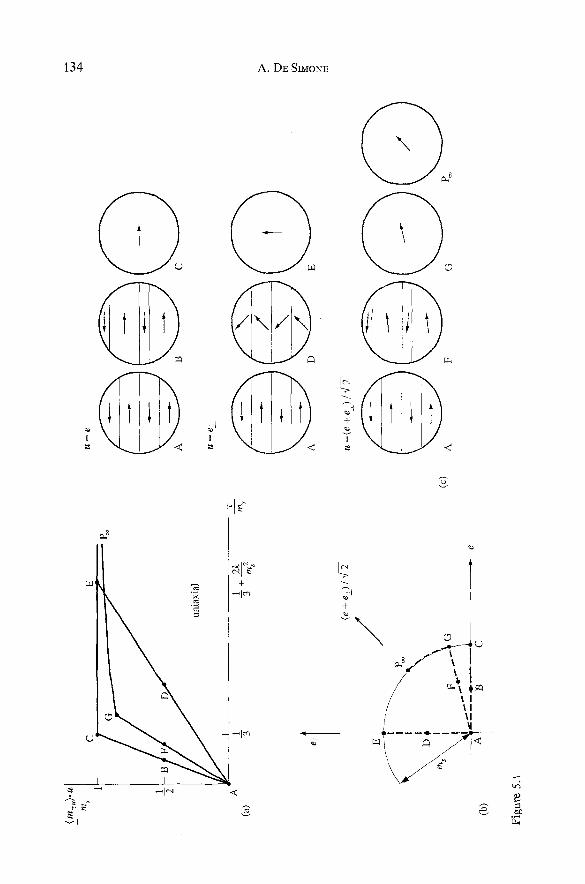
( m
Tu
) �9 I
I.
m s
A
(a)
(b)
C
E
G
P~
B F
unia
xial
1 1
2k
+ 3
m~
(e +
eL
) / ~
-
m s
u=
e
u=
e l
(c)
u =
(e +
e L
)/4-
2
a F
G
P
~
4~
> O
Fig
ure
5.1
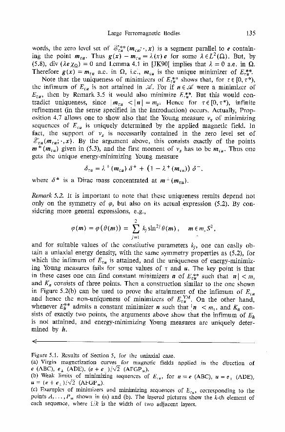
Large Ferromagnetic Bodies 135
words, the zero level set of ~ * * (m~u; ", x) is a segment parallel to e contain- ing the point m ~ . Thus g(x) - m ~ = 2(x) e for some 2 EL2(C2). But, by (5.8), div ()teza) = 0 and Lemma 4.1 in [JK90] implies that 2 = 0 a.e. in f2. Therefore g(x) = m~ a.e. in f2, i .e , m ~ is the unique minimizer of E**.
Note that the uniqueness of minimizers of E~** shows that, for r E [0, r*), the inf imum of E~u is not attained in S . For if n 6 d were a minimizer of E ~ , then by Remark 3.5 it would also minimize E~**. But this would con- tradict uniqueness, since [m~u[ < In[ = ms. Hence for r~ [0, r*), infinite refinement (in the sense specified in the Introduction) occurs. Actually, Prop- osition 4.7 allows one to show also that the Young measure v~ of minimizing sequences of E~u is uniquely determined by the applied magnetic field. In fact, the support of v~ is necessarily contained in the zero level set of ~u(m~u; ' ,x) . By the argument above, this consists exactly of the points
m • (m~,) given in (5.3), and the first moment of v~ has to be m~,. Thus one gets the Unique energy-minimizing Young measure
firu = 2+ (rn~u) fi+ + (1 - 2+ (m~,)) f i - ,
where fi• is a Dirac mass concentrated at m•
Remark 5.2. It is important to note that these uniqueness results depend not only on the symmetry of (0, but also on its actual expression (5.2). By con- sidering more general expressions, e.g.,
2
(p(m) = Co(O(m)) = ~ kjsin2JO(m), m ~ m , S 2, j = i "
and for suitable values of the constitutive parameters kj, one can easily ob- tain a uniaxial energy density, with the same symmetry properties as (5.2), for which the infimum of E~u is attained, and the uniqueness of energy-minimiz- ing Young measures fails for some values of r and u. The key point is that in these cases one can find constant minimizers n of E** such that I n [ < ms and Kn consists of three points. Then a construction similar to the one shown in Figure 5.2(b) can be used to prove the attainment of the infimum of E~u and hence the non-uniqueness of minimizers of YM E~u �9 On the other hand, whenever E~* admits a constant minimizer n such that I nl < ms, and K, con- sists of exactly two points, the arguments above show that the infimum of E h is not attained, and energy-minimizing Young measures are uniquely deter- mined by h.
<
Figure 5.1. Results of Section 5, for the uniaxial case. (a) Virgin magnetization curves for magnetic fields applied in the direction of e (ABC), e• (ADE), (e + e• (AFGP=). (b) Weak limits of minimizing sequences of E~u , for u = e (ABC), u = e• (ADE), u = (e + ez)/x/2 (AFGP~). (c) Examples of minimizers and minimizing sequences of E~u, corresponding to the points A . . . . . P= shown in (a) and (b). The layered pictures show the k-th element of each sequence, where l/k is the width of two adjacent layers.
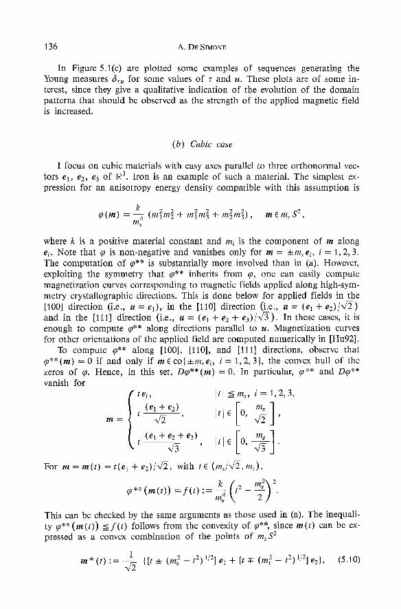
136 A. DE SIMONE
In Figure 5.1(c) are plotted some examples of sequences generating the Young measures fi~u for some values of r and u. These plots are of some in- terest, since they give a qualitative indication of the evolution of the domain patterns that should be observed as the strength of the applied magnetic field is increased.
(b) Cubic case
I focus on cubic materials with easy axes parallel to three orthonormal vec- tors el, e2, e3 of [R 3. Iron is an example of such a material. The simplest ex- pression for an anisotropy energy density compatible with this assumption is
k 2 2 2 2 2 2 ~o(rn) = 77a.4 (mlm2 + mlm3 + m2m3), m ~ ms S 2, ms
where k is a positive material constant and mi is the component of m along eg. Note that q~ is non-negative and vanishes only for rn = 4-msei, i = 1,2, 3. The computation of ~0"* is substantially more involved than in (a). However, exploiting the symmetry that ~0"* inherits from (p, one can easily compute magnetization curves corresponding to magnetic fields applied along high-sym- metry crystallographic directions. This is done below for applied fields in the [1001 direction (i.e., u = el) , in the [110] direction (i.e., u = (el + e2)/x/2) and in the [111] direction (i.e., u = (el + e2 q- e3)/x/3) . In these cases, it is enough to compute ~0"* along directions parallel to u. Magnetization curves for other orientations of the applied field are computed numerically in [Hu92].
To compute (o** along [100], [110], and [111] directions, observe that ~0**(m) = 0 if and only if mEco{-4-msei, i = 1,2,3}, the convex hull of the zeros of ~0. Hence, in this set, Dr = 0. In particular, (p** and D~0**
17l
vanish for
t ( e l + e 2 ) Itj~ O, ms '
[ t ( e l + e 2 + e s ) Itl 0, X/5 '
For m = re(t) = t(el + e2)/x/2, with tE (m~/x/2,ms),
k ( m~\ 2 ~0"* ( re( t ) ) =f(t):=--~ms t2 - 2 ) "
This can be checked by the same arguments as those used in (a). The inequali- ty fp** (m( t ) ) <=f(t) follows from the convexity of q)**, since re(t) can be ex- pressed as a convex combination of the points of ms S 2
1 m • x/2 {[t4- (m2s--t2)l/2]e~+[t-Y - (m2s--t2)V2]e2}, (5.10)
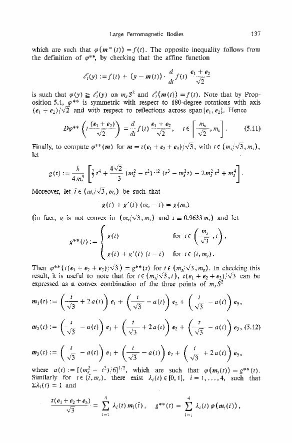
Large Ferromagnetic Bodies 137
which are such that (0(m--(t)) = f ( t ) . The opposite inequality follows from the definition of ~**, by checking that the affine function
d el + e2 ~t(Y) : = f ( t ) + (y - re(t)), d t f ( t )
is such that ~o(y) => ~ (y ) on m~S 2 and ~t(m(t)) = f ( t ) . Note that by Prop- osition 5.1, ~0"* is symmetric with respect to 180-degree rotations with axis (el + e2)/,]2 and with respect to reflections across span{el,e2}. Hence
((el-+~e2)-'~ d e l + e 2 [ ms ] O(o** t x/2 ] = ~ f ( t ) ~/~- , t~ ~ - , m s . (5.11)
Finally, to compute (o** (m) for m = t(el + e2 + e3)/x/3, with tE (ms/x/3, ms), let
k [ 4x/2 (m2s _ tz)1/z (t3 m2t) _ 2m2 tZ + m41. g ( t ) : - 4 m 4 7t 4+ 3
Moreover, let {~ (ms/,/3,ms) be such that
g({) + g'({) (m s - {) = g(m~)
(in fact, g is not convex in (ms/X[5, ms) and t -=- 0.9633 ms) and let
(m 0 g**(t) := g(t) for t~ ~ - , ,
g(T) + g ' ( i ) ( t - i ) for t ( (~ ,m~) .
Then ~0"* (t(el + e2 + e3)/", /3 ) = g** ( t) fo r t E (ms/'~/3, ms). In checking this result, it is useful to note that for t6 (ms/',/3, i) , t(el + e2 + e3)/ 'f3 can be expressed as a convex combination of the three points of ms S 2
( + 3 ) ( + ) ( + 3 ) ml(t) := + 2a( t ) e 1 + - a(t) e: + - a(t) e3,
( + ) ( + ) ( + ) me(t) := - a(t) e 1 + + 2a( t ) ee + - a(t) e3, (5.12)
( + ) ( + 3 , ) (+ ) m3(t) := - a(t) e l+ - a(t e2+ + 2 a ( t ) e3,
where a ( t ) : = [ ( m ~ - t 2 ) / 6 ] 1/2, which are such that o(mi(t) ) =g**( t ) . Similarly for t~(i ,m~), there exist 2 i ( t ) ( [0 ,1 ] , i = 1 . . . . . 4, such that s = 1 and
t ( e l + ee + e3) 4 4
,/5 i=l i=1
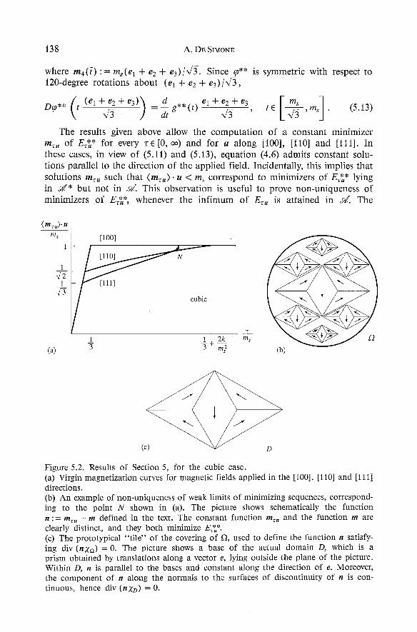
138 A. DE SIMONE
where m4(/) := ms(e 1 + e 2 + e3)/x/3. Since (0"* is symmetric with respect to 120-degree rotations about (e 1 + e2 + e3)/x/3,
D(o**(t (el+e2+e3)) dg**(t) el+e2+e3 [ms ] 7,~ = ~ ~ , tr ~ - , m s . (5.13)
The results given above allow the computat ion of a constant minimizer rn, , of E** for every rE [0, c~) and for u along [100], [ll0] and [1111. In these cases, in view of (5.11) and (5.13), equation (4.6) admits constant solu- tions parallel to the direction of the applied field. Incidentally, this implies that solutions m,u such that (rn~u). u < m, correspond to minimizers of E*** lying in d * but not in S . This observation is useful to prove non-uniqueness of minimizers o f E**, whenever the inf imum of E ~ is attained in S . The
(mTU)" U m s
1
1
[lOO]
cubic
I I ! 1 1 2k m=
3 + m 2 (a) s (b)
(c) D
Figure 5.2. Results of Section 5, for the cubic case. (a) Virgin magnetization curves for magnetic fields applied in the [100], [1101 and [1111 directions. (b) An example of non-uniqueness of weak limits of minimizing sequences, correspond- ing to the point N shown in (a). The picture shows schematically the function n : = m~u- m defined in the text. The constant function rn~u and the function m are clearly distinct, and they both minimize E**. (c) The prototypical "tile" of the covering of ~, used to define the function n satisfy- ing div (nza) = 0. The picture shows a base of the actual domain D, which is a prism obtained by translations along a vector e, lying outside the plane of the picture. Within D, n is parallel to the bases and constant along the direction of e. Moreover, the component of n along the normals to the surfaces of discontinuity of n is con- tinuous, hence div (nzD) = O.
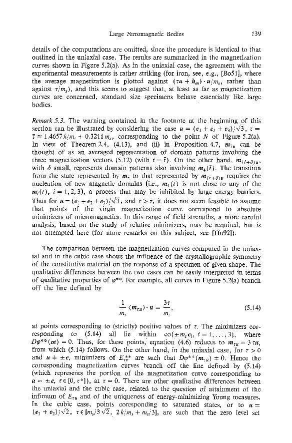
Large Ferromagnetic Bodies 139
details of the computations are omitted, since the procedure is identical to that outlined in the uniaxial case. The results are summarized in the magnetization curves shown in Figure 5.2(a). As in the uniaxial case, the agreement with the experimental measurements is rather striking (for iron, see, e.g., [Bo51], where the average magnetization is plotted against (ru + hm)" u/ms, rather than against "C/ms), and this seems to suggest that, at least as far as magnetization curves are concerned, standard size specimens behave essentially like large bodies.
Remark 5.3. The warning contained in the footnote at the beginning of this section can be illustrated by considering the case u = (el + e2 + e 3 ) / ~ , -c =
_~ 1.4657k/ms + 0.3211ms, corresponding to the point N of Figure 5.2(a). In view of Theorem 2.4, (4.13), and (ii) in Proposition 4.7, rn~ can be thought of as an averaged representation of domain patterns involving the three magnetization vectors (5.12) (with t = [). On the other hand, rn(~+~)u, with O small, represents domain patterns also involving m4(i ). The transition from the state represented by tn~ to that represented by m(~+~)u requires the nucleation of new magnetic domains (i.e., m4(t) is not close to any of the mi(i), i = 1, 2, 3), a process that may be inhibited by large energy barriers.
Thus for u = (el + e2 + e3)/x/3, and r > ~, it does not seem feasible to assume that points of the virgin magnetization curve correspond to absolute minimizers of micromagnetics. In this range of field strengths, a more careful analysis, based on the study of relative minimizers, may be required, but is not attempted here (for more remarks on this subject, see [Hu92]).
The comparison between the magnetization curves computed in the uniax- ial and in the cubic case shows the influence of the crystallographic symmetry of the constitutive material on the response of a specimen of given shape. The qualitative differences between the two cases can be easily interpreted in terms of qualitative properties of ~0"*. For example, all curves in Figure 5.2(a) branch off the line defined by
i 3z - - < m ~ u > " u = - - , ( 5 . 1 4 ) ms ms
at points corresponding to (strictly) positive values of r. The minimizers cor- responding to (5.14) all lie within co[=Lm sei, i = 1 . . . . . 3}, where D~o**(m) = 0. Thus, for these points, equation (4.6) reduces to rnru = 3 ru, from which (5.14) follows. On the other hand, in the uniaxial case, for T > 0 and u :r +e, minimizers of E** are such that D~o**(m~u) 3: O. Hence the corresponding magnetization curves branch off the line defined by (5.14) (which represents the portion of the magnetization curve corresponding to u = 4- e, r ~ [0, r*] ) , at r = 0. There are other qualitative differences between the uniaxial and the cubic case, related to the question of attainment of the infimum of E~, and of the uniqueness of energy-minimizing Young measures. In the cubic case, points coresponding to saturated states, or to u = (el + e2)/ ' ]2, T( [ms/3,~, 2k/ms + ms/31, are such that the zero level set
140 A. DE SIMONE
of ~ u ( m ~ u ; . , x ) is independent of x and consists of at most two points. Hence, in these cases, one has respectively attainment and uniqueness of minimizers, and non-attainment and uniqueness of energy minimizing Young measures (see Remark 5.2). However, an obvious minimizer of E~'* is m = 0, and Figure 2 in [JK90] illustrates the existence of elements of S that minimize E0. Thus, for z = 0, the infimum of E,u is attained, and energy-minimizing Young measures are not uniquely determined by the applied magnetic field. Figure 5.2(b) provides a further example in this direction, corresponding to u = (e 1 + e2 + e3)/x/3, "c = ~" (i.e., to the point N of Figure 5.2(a)). The picture schematically shows the function n : = tn~u - m, where m fi S takes on only the values mi(Z), i = 1, 2, 3, given by (5.12), which are in the zero level set of ~z~(mr , ; . , x ) . The function n is constructed by covering g) in the sense of Vitali (see [JK90]) with scaled copies of the domain D shown in Figure 5.2(c), on which n is defined so that div ( n z D ) = 0. Arguing as in [JKg0], implies that div ( n z n ) = 0. Thus m ~ S minimizes E**, and since rn:, ff S , non-uniqueness follows. Further examples of attainment of the in- fimum of E~,, leading to non-uniqueness of energy-minimizing Young measures, are illustrated by the self-similar constructions shown in [Pr76, pages 51 and 54].
The non-uniqueness of minimizers of El** brings us back to the issue of finding a selection criterion for minimizing sequences of Er~. However, this question, which is relevant for the detailed prediction of domain patterns, is immaterial for the prediction of limit magnetization curves corresponding to absolute minimizers of the micromagnetics functional. After all, the whole point of proving Proposition 4.5 is to be able to stop the computations here.
Appendix: magnetostatics
A magnetized ferromagnetic body, occupying the region f~ C ~3, and with magnetization m, generates a magnetic field satisfying Maxwell's equations for magnetostatics in the absence of currents, namely,
curl hm = O]
) div (h m + m x n ) 0 in N3. (A.1)
Here Za is the characteristic function of f~, which [ assume to be open, bounded and with Lipschitz boundary, and m z a is the extension of m to N3 that vanishes outside f~. To give a precise meaning to (A.1), let m EL2(r fir 3) be given. Then hm is defined as the element of
~'~:= {h EL2(R 3, ~3) : curlh = 0 in fir 3 in the sense of distributions}
satisfying
I hm" h = -- ~ mzf~" tt Vh E ~ . (A.2) ~3 R 3
Large Ferromagnetic Bodies 141
Alternatively, since h 6LZ(N 3, R 3) is curl-free in R 3 if and only if there exists ~ H 1(~3) such that h = - V ~ , (A.2) is equivalent to
j V~m" V~ = j mxa. Vr VCEHI(R3), (A.3) R3 ~3
where ~,~ fi H 1 (R 3) and Vg~ m = - hm. The Lax-Milgram lemma guarantees the existence and uniqueness of solutions of (A.2) in X . Thus the operator ~ such that hm = A'[mza] is well defined, and one can show that ,~ is a linear, con- tinuous and hence weakly continuous operator mapping L2(f2, ~3) into Z (see [JK90], [Ro911). Therefore, if m ~ m in L2(f2, R 3) as k--* co, then
S lhml 2 lim I h 2. = I mk I (A.4) IR 3 k-~oo ~3
Moreover, from the weak continuity of ~, in view of the weak lower semicon- tinuity of norms, it follows that if rnk~rn in L2(f2, R 3) as k--,co, then
j lhml 2 ~ liminf j Ihmkl 2, (A.5) Rs k~ec ~s
i.e., the magnetostatic energy is weakly lower semicontinuous. Note, however, that the magnetostatic energy is not weakly continuous.
For m and m' in L2(f2, R3), the following useful identities are a direct consequence of (A.2):
1 J i ,([mza][2 = - �89 J rnza ~ [ m z a ] , (A.6) IR 3 R3
J mza" ,4'[m'za] = j Z[mxnl" m'zn. (A.7) ~3 ~3
Then from (A.6) and (A.7), using the linearity of ~ one gets
i j {ihm, i 2 2 I - Ihml = - j ( m ' - m ) ' h m + � 8 9 2 (A.8) ~3 f~ ~3
An important property of ,4' is that if f2 is an ellipsoid and m is constant, then ,~[mza] is also constant in ~, i.e., uniformly magnetized ellipsoids in- duce uniform magnetic fields in their interiors. In particular, if f2 is spherical, then for every vector mo ~ R 3
~[moZa] (x) = - �89 a.e. in f2. (A.9)
Acknowledgements. This work is part of my doctoral dissertation, and has been partially supported through NSF/DMS-9111572, AFOSR-91-0301, ONR N/NOO14-9t-J-4034, ARO DAAL03-92-G003. It gives me great pleasure to express my gratitude to my ad- visor RICHARD D. JAMES for the enthusiasm and insight with which he has guided my efforts. I am also grateful to J. M. BAL~, N. B. FIROOZYE, G. FRIESECKE and V. SVERAK for many discussions and suggestions, and to S. M~2L~ER for some enlightening conver- sations. I thank Professor A. HUBERT for helpful discussions after my presentation of these results at the ICMS workshop on "Micromagnetics and Magnetostriction"
142 A. DE SIMONE
(Heriot-Watt University, Edinburgh, June 1992), for calling my attention to references [N644] and [LS48] and for allowing me to read parts of his unpublished manuscript [Hu921. Finally, I thank P. PEDREGAL, since an exchange of drafts of our papers led to various improvements in the exposition of the results of Sections 3 and 4.
[AB90]
[AV91]
[Ah88]
[BJ92]
[BK90I
[Bo51] [Br62]
[Br63] [Br69]
[BR92]
[Bz87] [Ch64] IDa89]
[De92] [Er91]
[ET76]
[Fr92]
[Hu67]
[Hu921 [JK90]
[JK92]
[JM92]
[KM92]
R e f e r e n c e s
G. ANZELLOTTI & S. BALDO: Asymptotic development by F-convergence. Preprint (1990). G. ANZELLOTTI, S. BALDO & A. VISINTIN: Asymptotic behavior of the Landau- Lifschitz model of ferromagnetism. Appl. Math. and Opt. 23 (1991), 171-192. A. AHARONI: Elongated single domain particles. J. Appl. Phys. 63 (1988), 5879- 5882. J. M. BALL & R. D. JAMES: Proposed experimental tests of a theory of fine microstructure and the two-well problem. Phil. Trans. R. Soc. Lond. A338 (1992), 389-450. J. M. BALL & G. KNOW~ES: Young measures and minimization problems of mechanics. In: Elasticity: mathematical methods and applications (G. EASON & R. W. OGDEN eds.). Ellis Horwood, Chichester, 1990. R. M. BOZORTI-I: Ferromagnetism. Van Nostrand, Princeton, 1951. W. E BROWN: Magnetostatic Principles in Ferromagnetism. North-Holland, Amsterdam, 1962. W. F. BROWN: Micromagnetics. Wiley, New York, 1963. W. E BROWN: The fundamental theorem of the theory of fine ferromagnetic particles. Ann. New York Acad. Sci. 147 (1969), 463-488. D. BRANDON & R. C. ROGERS: The coercivity paradox and nonlocal fer- romagnetism. Cont. Mech. Therm. 4 (1992), 1-21 . H. BREZlS: Analyse Fonctionelle. Masson, Paris, 1987. S. CmKaZUMI: Physics of Magnetism. Wiley, New York, 1964. B. DACOROGNA: Direct Methods in the Calculus of Variations. Springer-Verlag, Berlin, 1989. A. DE SIMONE: Thesis. University of Minnesota (1992). J. L. ERICKSEN: Introduction to the Thermodynamics of Solids. Chap- man & Hall, London, 1991. I. EKELAND • R. TEMAM: Convex Analysis and Variational Problems. North- Holland, Amsterdam, 1976. G. FRIESECI(E: A necessary and sufficient condition for non attainment and formation of microstructure almost everywhere in scalar variational problems. Proc. Roy. Soc. Edin. A. To appear. A. HUBERT: Znr Theorie der zweiphasigen Dom~inenstrukturen in Supraleitern und Ferromagneten. Phys. Stat. Sol. 24 (1967), 669-682. A. HUBERT: Magnetic Domains. In preparation. R. D. JAMES ~; D. KINDERLEI-IRER: Frustration in ferromagnetic materials. Cont. Mech. Therm. 2 (1990), 215-239. R. D. JAMES & D. KINDERLEHRER: Theory of magnetostriction with applica- tions to TbxDyl-xFe2. Phil. Mag. B. To appear. R. D. JAMES & S. M~ILLER: Internal variables and fine scale oscillations in Micromagnetics. Cont. Mech. Therm. To appear. R. V. KOI-IN & S. MOILER: Branching of twins near an austenite/twinned- martensite interface. Phil. Mag. A 66 (1992), 697-715.
Large Ferromagnetic Bodies 143
[KT85]
[Li44]
[LL35]
[LM921
[LS48]
[Ma91] [Mti90]
[Mii92]
[N644]
[Pe92] [Pr76]
[Rk70] [Ro91]
[SW481
[Tag01
[Ta91] [Ta921
[Vr891
[Vs851
[Yo801
[Zi671
K. C. KooN, B. N. DAS, M. RUBINSTEIN & J. TYSON: Magnetic properties of R2Fe14B single crystals. J. Appl. Phys. 57 (1985), 4091-4093. E. M. LIFSCHITZ: Oil the magnetic structure of iron. J. Phys. USSR 8 (1944), 337-346. L. D. LANDAU & E. M. LIFSCHITZ: On the theory of the dispersion of magnetic permeability in ferromagnetic bodies. Phys. Z. Sowjetunion 8 (1935), 153-169. M. LUSKIN & LING MA: Analysis of the finite element approximation of microstructure in micromagnetics. SIAM J. Num. Anal. 9 (1992), 320-331. H. LAWTON & K. H. STEWART: Magnetization curves for ferromagnetic single crystals. Proc. Roy. Soc. Lond. A193 (1948), 72-88. LING MA: Thesis. University of Minnesota (1991). S. MOLLER: Minimizing sequences for nonconvex functionals, phase transi- tions and singular perturbations. In: Problems involving change of type. (K. KIRCI-IG~-SSNER, ed.) Springer Lecture Notes in Physics 359 (1990), 31-44. S. MOILER: Singular perturbation as a selection criterion for periodic minimizing sequences. Calculus of Variations. To appear. L. Ns Les lois de l'aimantation et de la subdivision en domaines 616men- taires d'un monocristal de fer I - I I I . J. Phys. Rad. S (1944), 241-251, 265 -276. P. PEDREGAL: Relaxation in ferromagnetism: the rigid case. To appear. I. PRIVOROTSKn: Thermodynamic theory of domain structures. Wiley, New York, 1976. T. ROCKAFEL~AR: Convex Analysis. Princeton University Press, 1970. R. C. ROGERS: A nonlocal model for the exchange energy in ferromagnetic materials. J. Int. Eq. Appl. 3 (1991), 85-127. E. C. STONER & E. P. WOLLFARTH: A mechanism of magnetic hysteresis in heterogeneous alloys. Phil. Trans. Roy. Soc. Lond. A240 (1948), 599-642. L. TARTAR: H-measures, a new approach for studying homogeneisation, oscillations and concentration effects in partial differential equations. Proc. Roy. Soc. Edin. l lSA (1990), 193-230. L. TARTAR: Personal communication to R. D. James. December 1991. L. TARTAR: On mathematical tools for studying partial differential equations of continuum physics: H-measures and Young measures. Preprint (1992). E. VmoA: Drops of nematic liquid crystals. Arch. Rational Mech. Anal. 107 (1989), 371-390. A. VISINTIN: On Landau-Lifschitz' equations for ferromagnetism. Jap. J. Appl. Math. 2 (1985), 69-84. L. C. YOUNG: Lectures on Calculus of Variations and Optimal Control Theory. Chelsea, New York, 1980. H. ZlJ'LSTRA: Experimental Methods in Magnetism. Vols. 1, 2. North-Holland, Amsterdam, 1967.
Dipartimento di Ingegneria Civile Universit/t di Roma "Tor Vergata"
00133 Roma
(Accepted January29, 1993)