Embed Size (px)
Citation preview
Page | 1
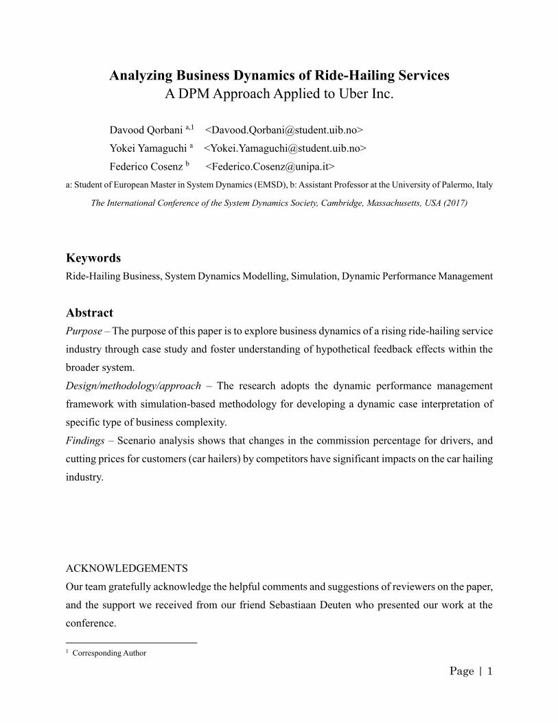
Analyzing Business Dynamics of Ride-Hailing Services
A DPM Approach Applied to Uber Inc.
Davood Qorbani a,1 <[email protected]>
Yokei Yamaguchi a <[email protected]>
Federico Cosenz b <[email protected]>
a: Student of European Master in System Dynamics (EMSD), b: Assistant Professor at the University of Palermo, Italy
The International Conference of the System Dynamics Society, Cambridge, Massachusetts, USA (2017)
Keywords
Ride-Hailing Business, System Dynamics Modelling, Simulation, Dynamic Performance Management
Abstract
Purpose – The purpose of this paper is to explore business dynamics of a rising ride-hailing service
industry through case study and foster understanding of hypothetical feedback effects within the
broader system.
Design/methodology/approach – The research adopts the dynamic performance management
framework with simulation-based methodology for developing a dynamic case interpretation of
specific type of business complexity.
Findings – Scenario analysis shows that changes in the commission percentage for drivers, and
cutting prices for customers (car hailers) by competitors have significant impacts on the car hailing
industry.
ACKNOWLEDGEMENTS
Our team gratefully acknowledge the helpful comments and suggestions of reviewers on the paper,
and the support we received from our friend Sebastiaan Deuten who presented our work at the
conference.
1 Corresponding Author
Page | 2
Introduction
Uber Inc. (hereafter called Uber), since its foundation in March 2009, has experienced significant
growth during recent years both internally and externally. Internally speaking, the company has
been successful in expanding its service capacity in all the cities where it operates. Externally
speaking, Uber has been strategic in developing not only its company name-value, but also in
acquiring additional funds. Recent Uber’s strategic partnership with Toyota (U.S.)
(Bloomberg.com, 2016), a top global automobile company, shows the on-going business dynamics
of the company and prospective business future. At the same time, market valuation of the
company shows an outstanding growth, which could be interpreted as one of clear indicators of
such excitement and business expectation.
Uber’s core business is providing a market for the ride-hailing service supported by
point-to-point software technology and mobile phone application, connecting drivers and
passengers. In this paper, based on the “qualitative” case study “Uber: Changing the Way the World
Moves” (Moon, 2015), we attempted to interpret this business-specific case study from
management decisions perspective, through System Dynamics “quantitative” modeling approach.
Particularly we focused on the company’s business area in New York City. The concept
used in Dynamic Performance Management (hereafter called DPM) is also utilized to foster the
understanding of complex, multilayer factors affecting its core business area. To the best of our
knowledge, such a research attempt has not been performed or made available so far, which
became one of our challenges to overcome in this research together with limited available data due
to the company’s private status.
Critical factors impacting on Performance Management design and
implementation
In recent years, simulation as a research method has gained attraction, allowing for the analysis of
complex strategic phenomena that incorporate a multitude of interrelated issues which may lead
to inflexible analytical models and are particularly difficult to manage in empirical research.
Conventional Performance Management (PM) systems represent useful tools to drive
decision-makers in both designing competitive strategies and measuring resulting outcomes.
However, they often lack to capture the dynamic complexity of managerial decision-making. In
fact, they may fail to consider a number of relevant factors influencing organizational performance.
Such factors can be associated to delays, non-linearity, intangibles, to the unintended consequences
Page | 3
on human perceptions, and to a behavior caused by a superficial or mechanistic approach in setting
performance targets, especially if such targets are used as a basis for organizational incentive and
career systems. In addition, these PM systems tend to frame business performance from a too static
point of view that does not allow one to properly assess policy impacts with reference to the trade-
offs existing between both short- vs. long-term effects (time), and results related to different
strategic business and functional areas within an organization (space). This implies a weak
understanding of both the impact of current decisions on future growth and the strategy to
undertake to cope with major changes. As De Geus (1997) found, misperceiving dynamic
complexity is a main cause of poor organizational performance and crisis. For instance, despite its
widely recognized advantages, even the Balanced Scorecard (BSC) by Kaplan and Norton (1996)
presents some conceptual and structural shortcomings. Linard et al. (2002) assert that the BSC
fails to translate company strategy into a coherent set of measures and objectives, because it lacks
a rigorous methodology for selecting metrics and for establishing the relationship between metrics
and firm strategy. Sloper et al. (1999) remark that the BSC is a static approach. Although Kaplan
and Norton stress the importance of feedback relationships between BSC variables for describing
the trajectory of a given strategy, the cause-and-effect chain is always conceived as a bottom-up
causality, which totally ignores feedbacks, thereby confining attention only to the effect of
variables in the lower perspectives (Linard and Dvorsky, 2001). Misperceiving the dynamic
relationships between the system’s feedback structure and behavior (Davidsen, 1996; Sterman,
2000) often leads managers to make their decisions according to a linear, static and bounded point
of view, in terms of time horizon and relationships between variables. Therefore, conventional
approaches to PM may limit decision-makers’ strategic learning processes (Sloper et al., 1999;
Linard and Dvorsky, 2001) and, as a result, impoverish management decision effectiveness.
As a result, a “dynamic” perspective in designing and implementing PM systems is
particularly valuable in complex and unpredictable contexts, as it implies the identification and
analysis of end-results, value drivers and related strategic resources accumulation/depletion
processes, according to a “cause-and-effect” perspective. A feedback analysis may allow decision-
makers to better frame the relevant structure underlying performance and, consequently, to design
and assess a set of alternative strategies to adopt, so to affect the system structure according to the
desired performance behavior.
In recent years, System Dynamics (SD) modelling combined with strategic PM systems
hold promise to be effective in fostering strategic learning processes and, as a result, supporting

Page | 4
decision-making and performance improvement according to a systemic perspective (Bianchi,
2002, 2012; Bianchi et al., 2015; Cosenz and Noto, 2016). This approach, known as Dynamic
Performance Management (DPM), aims at supporting decision-making through a better
coordination between performance measurement reporting and strategy design (Bianchi, 2016;
Bianchi et al., 2015). In fact, the application of SD to PM helps business analysts to trace both
causes and drivers that have led to a given performance level over time and, in doing so, contributes
in enhancing the diagnosis process that enables business managers to put in place corrective
actions and strategies oriented to fill the gap between the actual and the target performance value.
In the next sections, this paper analyzes how SD modelling may add value to PM in
Ride-Hailing Services operating in dynamic and complex contexts. To this end, the Uber Inc. case-
study will be illustrated and discussed to provide empirical evidence on the effectiveness of this
approach to management decision and control.
Research Methodology: A DPM approach to analyze Ride-Hailing Service
Business Dynamics
To identify and analyze causal relationships underlying ride-hailing business performance
dynamics with the intent to understand how the company reacts to alternative strategies, we take
advantage of the combination between conventional PM tools (Neely, 1999; Neely et al., 1997;
Otley, 1999; Kaplan and Norton, 1996) and SD methodology (Forrester, 1961; Sterman, 2000).
In particular, conventional PM systems aim at managing organizational performance
through a perspective that focuses on end-results in order to design a selected, though significant,
set of performance drivers. These drivers represent not only useful measures of performance, but
also strategic levers on which to intervene in order to fill the gap between actual and expected
results. To affect such drivers, managers must build up, preserve, and deploy a proper endowment
of strategic resources. The feedback loops underlying the dynamics of the different strategic
resources imply that the flows affecting such resources depend on end-results and are measured
over a time lag. End-results are modelled as in- or out-flows, which over a given time span, change
the corresponding stocks of strategic resources, as the result of actions implemented by decision-
makers (Bianchi, 2016). For instance, liquidity (a strategic resource) may change as an effect of
cash flow (an end-result); the change in the image of a firm (an end-result) may change as an effect
of its customer satisfaction (a strategic resource).
On the other hand, SD is an approach for modelling and simulating complex physical
Page | 5
and social systems, and experimenting with the models to design policies for management and
change (Forrester, 1961). As such, SD modelling is adopted to map system structure to capture and
communicate an understanding of behavior driving processes and the quantification of the
relationships to produce a set of equations that form the basis for simulating possible system
behaviors over time. SD models are powerful tools to help understand and leverage the feedback
interrelationships of complex management systems. They are based on a feedback view of business
systems, seen as a closed boundary, i.e. embodying all the main variables related to the
phenomenon being investigated. These models offer an operational methodology to support
decision-making and management. Decision-makers can use the models to test alternative
scenarios and explore what might have happened – or what could happen – under a variety of
different past and future assumptions and across alternative decision choices (Sterman, 2000).
Model structures are realized by linking those relevant variables, which determine certain behavior
of the observed system over time. In these connections, feedback loops are the main building
blocks for articulating the dynamics of these models and their interactions can explain the system
behavior (Morecroft, 2007).
In comparison to other methodologies, the use of SD modelling may lead to remarkable
results in terms of identifying and analyzing both determinants and implications of a given
business phenomenon. As such, SD methodology frames the complex interactions among feedback
loops, rejects notions of linear cause-and-effect, and requires the analyst to view a complete system
of relationships whereby the “cause” might also be affected by the “effect”. This means that a
variable – other conditions being equal – influences another variable (1) positively (i.e., an increase
of the one corresponds to an increase of the other and vice-versa), (2) negatively (i.e., an increase
of the one corresponds to a decrease of the other and vice-versa), and (3) according to a non-linear
relation between them. In addition, if such relations originate closed circuits, these are defined as
feedback loops and determine the system behavior. Shortly, reinforcing loops (R) produce
exponential trends of the system over time; while, balancing loops (B) limit such an effect by
tending to a steady state. The underlying principle is that if the process structure determines the
system behavior, and the system behavior determines the business performance (Davidsen, 1991;
Richardson and Pugh, 1981; Sterman, 2000), then the key to developing sustainable strategies to
optimize performance is understanding the relationship between processes and behaviors and
managing the leverage points (Ghaffarzadegan et al., 2011). By framing the dynamics of a complex
business system, including interactions among key-actors, actions, organizational structures and
Page | 6
processes, analysts can better decide how to reinforce positive factors or diminishing the negative
pressures exerted upon them. Therefore, SD allows managers and entrepreneurs to link strategy to
action, to better perceive interdependencies between business units and functions, as well as
between the firm and its environment, and to understand the crucial role of strategic resources on
firm performance and survival. Therefore, combining SD and PM enables one not only to capture
causal relationships underlying the functioning of a business system, but also to simulate
performance behavior over time and, as a result, contributes in evaluating the trade-offs between
short- and long-term outcomes related to the adoption of a given strategy.
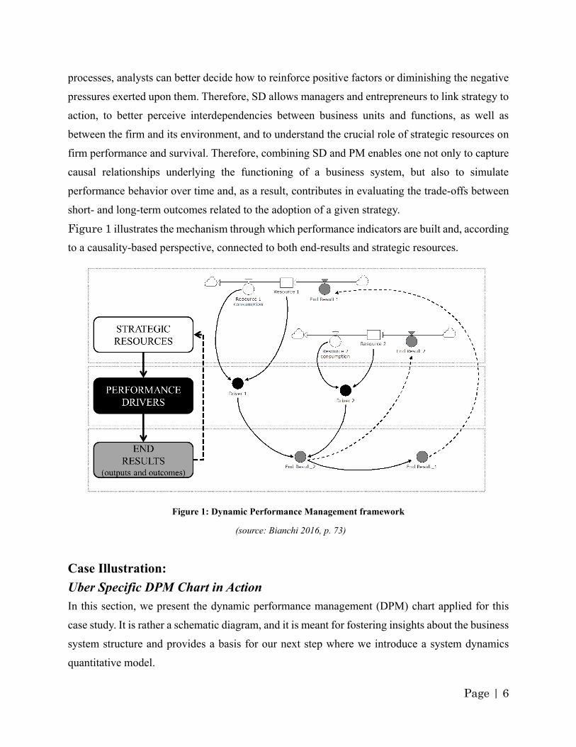
Figure 1 illustrates the mechanism through which performance indicators are built and, according
to a causality-based perspective, connected to both end-results and strategic resources.
Figure 1: Dynamic Performance Management framework
(source: Bianchi 2016, p. 73)
Case Illustration:
Uber Specific DPM Chart in Action
In this section, we present the dynamic performance management (DPM) chart applied for this
case study. It is rather a schematic diagram, and it is meant for fostering insights about the business
system structure and provides a basis for our next step where we introduce a system dynamics
quantitative model.
Page | 7
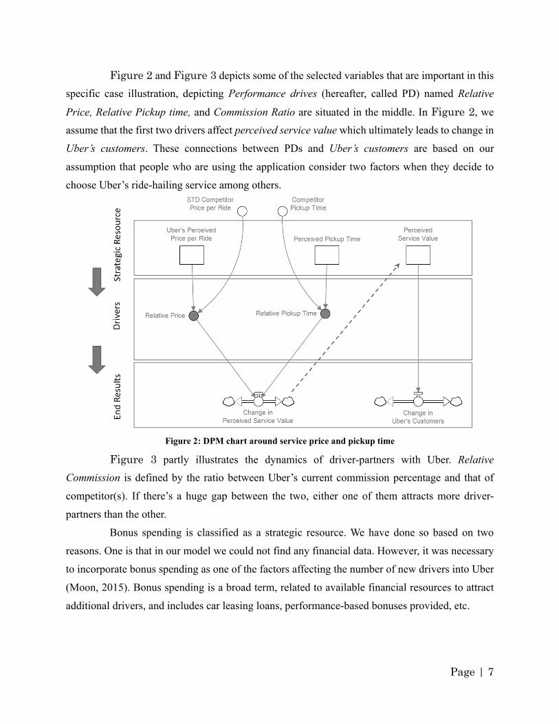
Figure 2 and Figure 3 depicts some of the selected variables that are important in this
specific case illustration, depicting Performance drives (hereafter, called PD) named Relative
Price, Relative Pickup time, and Commission Ratio are situated in the middle. In Figure 2, we
assume that the first two drivers affect perceived service value which ultimately leads to change in
Uber’s customers. These connections between PDs and Uber’s customers are based on our
assumption that people who are using the application consider two factors when they decide to
choose Uber’s ride-hailing service among others.
Figure 2: DPM chart around service price and pickup time
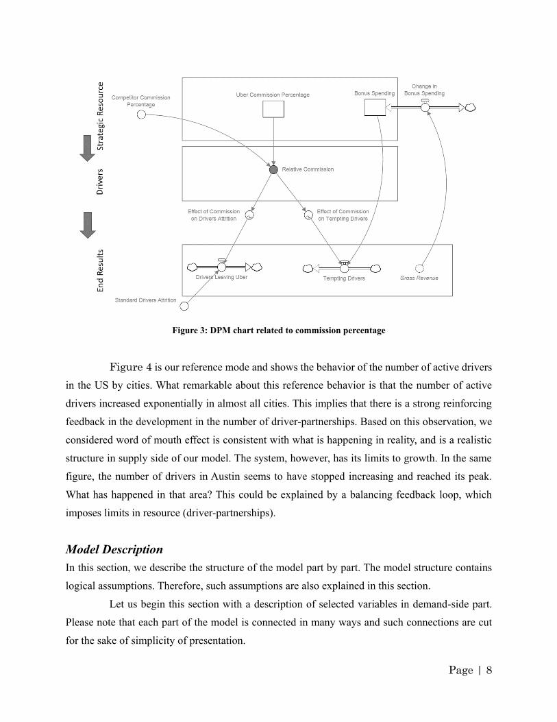
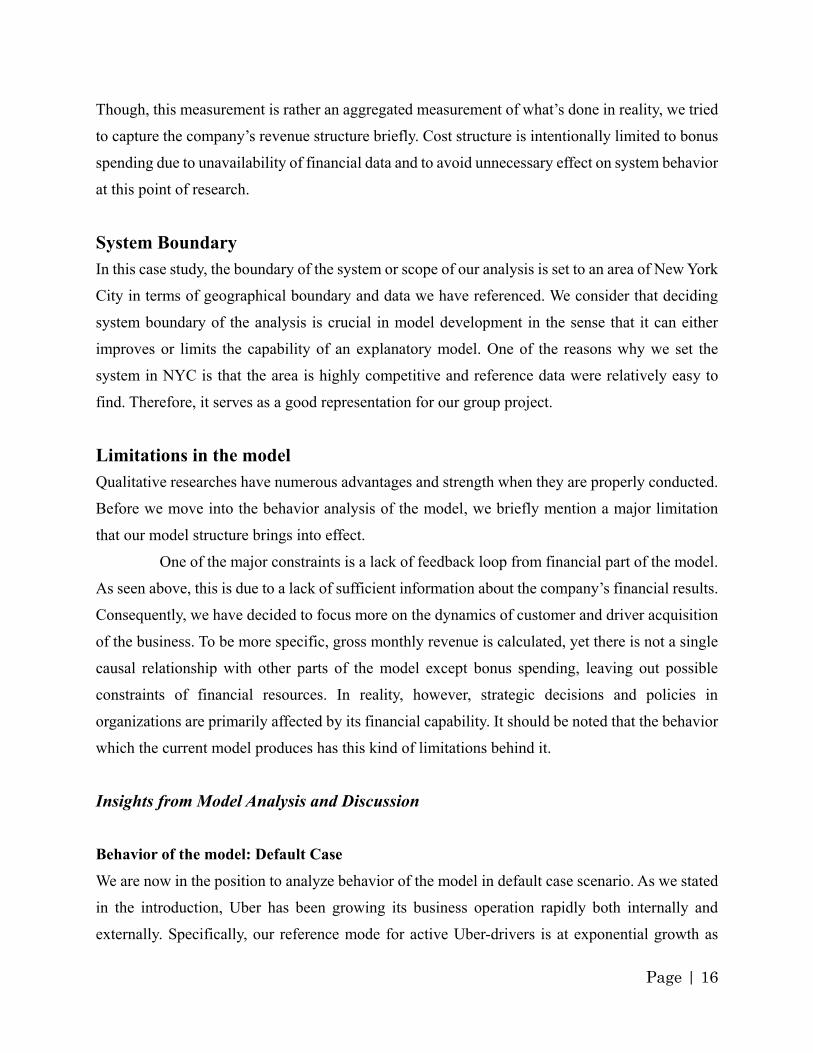
Figure 3 partly illustrates the dynamics of driver-partners with Uber. Relative
Commission is defined by the ratio between Uber’s current commission percentage and that of
competitor(s). If there’s a huge gap between the two, either one of them attracts more driver-
partners than the other.
Bonus spending is classified as a strategic resource. We have done so based on two
reasons. One is that in our model we could not find any financial data. However, it was necessary
to incorporate bonus spending as one of the factors affecting the number of new drivers into Uber
(Moon, 2015). Bonus spending is a broad term, related to available financial resources to attract
additional drivers, and includes car leasing loans, performance-based bonuses provided, etc.
Page | 8
Figure 3: DPM chart related to commission percentage
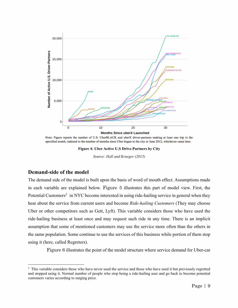
Figure 4 is our reference mode and shows the behavior of the number of active drivers
in the US by cities. What remarkable about this reference behavior is that the number of active
drivers increased exponentially in almost all cities. This implies that there is a strong reinforcing
feedback in the development in the number of driver-partnerships. Based on this observation, we
considered word of mouth effect is consistent with what is happening in reality, and is a realistic
structure in supply side of our model. The system, however, has its limits to growth. In the same
figure, the number of drivers in Austin seems to have stopped increasing and reached its peak.
What has happened in that area? This could be explained by a balancing feedback loop, which
imposes limits in resource (driver-partnerships).
Model Description
In this section, we describe the structure of the model part by part. The model structure contains
logical assumptions. Therefore, such assumptions are also explained in this section.
Let us begin this section with a description of selected variables in demand-side part.
Please note that each part of the model is connected in many ways and such connections are cut
for the sake of simplicity of presentation.
Page | 9
Figure 4: Uber Active U.S Drive-Partners by City
Source: Hall and Krueger (2015)
Demand-side of the model
The demand side of the model is built upon the basis of word of mouth effect. Assumptions made
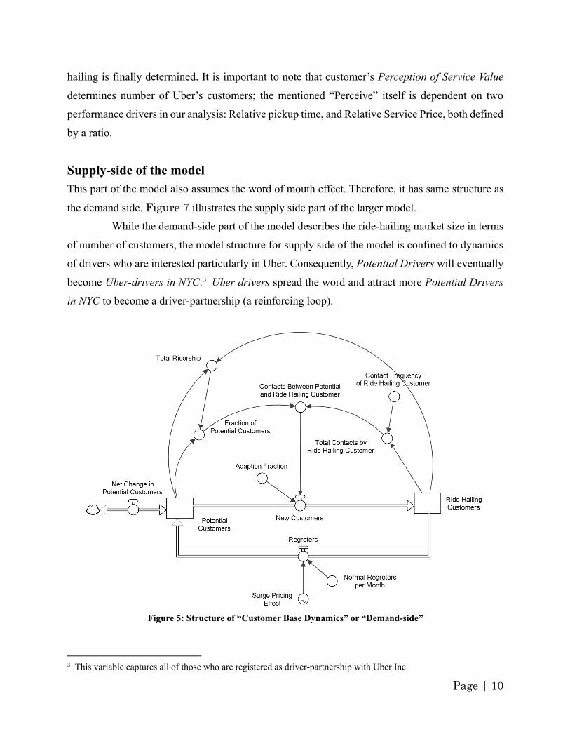
in each variable are explained below. Figure 5 illustrates this part of model view. First, the
Potential Customers2 in NYC become interested in using ride-hailing service in general when they
hear about the service from current users and become Ride-hailing Customers (They may choose
Uber or other competitors such as Gett, Lyft). This variable considers those who have used the
ride-hailing business at least once and may request such ride in any time. There is an implicit
assumption that some of mentioned customers may use the service more often than the others in
the same population. Some continue to use the services of this business while portion of them stop
using it (here, called Regreters).
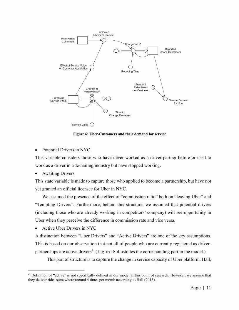
Figure 6 illustrates the point of the model structure where service demand for Uber-car
2 This variable considers those who have never used the service and those who have used it but previously regretted
and stopped using it. Normal number of people who stop being a ride-hailing user and go back to become potential
customers varies according to surging price.
Page | 10
hailing is finally determined. It is important to note that customer’s Perception of Service Value
determines number of Uber’s customers; the mentioned “Perceive” itself is dependent on two
performance drivers in our analysis: Relative pickup time, and Relative Service Price, both defined
by a ratio.
Supply-side of the model
This part of the model also assumes the word of mouth effect. Therefore, it has same structure as
the demand side. Figure 7 illustrates the supply side part of the larger model.
While the demand-side part of the model describes the ride-hailing market size in terms
of number of customers, the model structure for supply side of the model is confined to dynamics
of drivers who are interested particularly in Uber. Consequently, Potential Drivers will eventually
become Uber-drivers in NYC.3 Uber drivers spread the word and attract more Potential Drivers
in NYC to become a driver-partnership (a reinforcing loop).
Figure 5: Structure of “Customer Base Dynamics” or “Demand-side”
3 This variable captures all of those who are registered as driver-partnership with Uber Inc.
Page | 11
Figure 6: Uber-Customers and their demand for service
• Potential Drivers in NYC
This variable considers those who have never worked as a driver-partner before or used to
work as a driver in ride-hailing industry but have stopped working.
• Awaiting Drivers
This state variable is made to capture those who applied to become a partnership, but have not
yet granted an official licensee for Uber in NYC.
We assumed the presence of the effect of “commission ratio” both on “leaving Uber” and
“Tempting Drivers”. Furthermore, behind this structure, we assumed that potential drivers
(including those who are already working in competitors’ company) will see opportunity in
Uber when they perceive the difference in commission rate and vice versa.
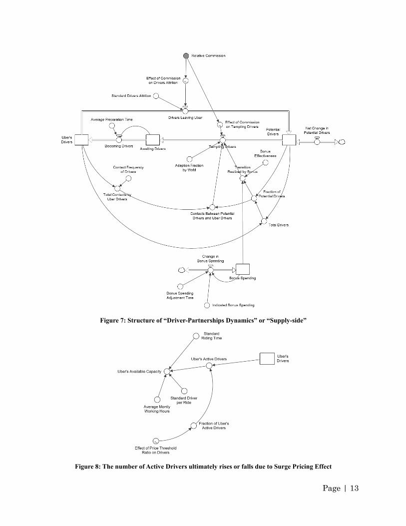
• Active Uber Drivers in NYC
A distinction between “Uber Drivers” and “Active Drivers” are one of the key assumptions.
This is based on our observation that not all of people who are currently registered as driver-
partnerships are active drivers4 (Figure 8 illustrates the corresponding part in the model.)
This part of structure is to capture the change in service capacity of Uber platform. Hall,
4 Definition of “active” is not specifically defined in our model at this point of research. However, we assume that
they deliver rides somewhere around 4 times per month according to Hall (2015).
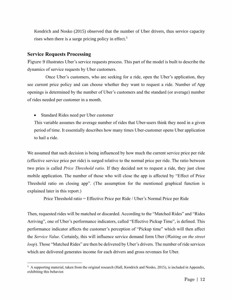
Page | 12
Kendrich and Nosko (2015) observed that the number of Uber drivers, thus service capacity
rises when there is a surge pricing policy in effect.5
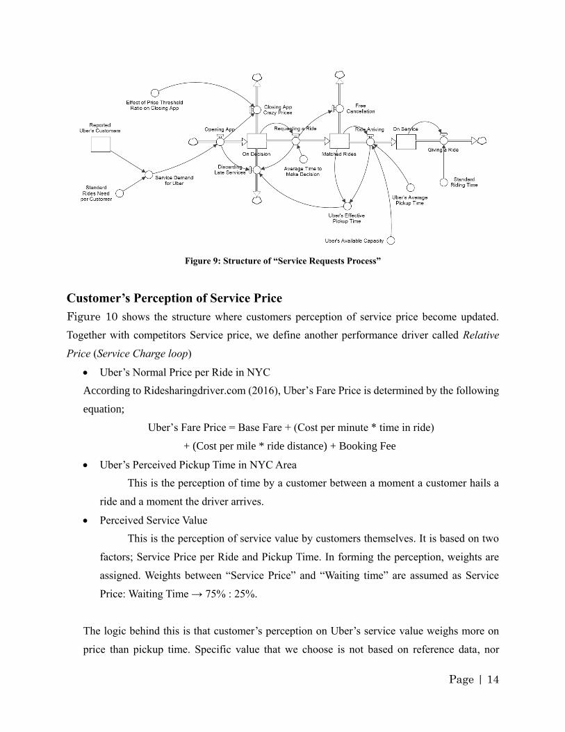
Service Requests Processing
Figure 9 illustrates Uber’s service requests process. This part of the model is built to describe the
dynamics of service requests by Uber customers.
Once Uber’s customers, who are seeking for a ride, open the Uber’s application, they
see current price policy and can choose whether they want to request a ride. Number of App
openings is determined by the number of Uber’s customers and the standard (or average) number
of rides needed per customer in a month.
• Standard Rides need per Uber customer
This variable assumes the average number of rides that Uber-users think they need in a given
period of time. It essentially describes how many times Uber-customer opens Uber application
to hail a ride.
We assumed that such decision is being influenced by how much the current service price per ride
(effective service price per ride) is surged relative to the normal price per ride. The ratio between
two pries is called Price Threshold ratio. If they decided not to request a ride, they just close
mobile application. The number of those who will close the app is affected by “Effect of Price
Threshold ratio on closing app”. (The assumption for the mentioned graphical function is
explained later in this report.)
Price Threshold ratio = Effective Price per Ride / Uber’s Normal Price per Ride
Then, requested rides will be matched or discarded. According to the “Matched Rides” and “Rides
Arriving”, one of Uber’s performance indicators, called “Effective Pickup Time”, is defined. This
performance indicator affects the customer’s perception of “Pickup time” which will then affect
the Service Value. Certainly, this will influence service demand form Uber (Waiting on the street
loop). Those “Matched Rides” are then be delivered by Uber’s drivers. The number of ride services
which are delivered generates income for each drivers and gross revenues for Uber.
5 A supporting material, taken from the original research (Hall, Kendrick and Nosko, 2015), is included in Appendix,
exhibiting this behavior.
Page | 13
Figure 7: Structure of “Driver-Partnerships Dynamics” or “Supply-side”
Figure 8: The number of Active Drivers ultimately rises or falls due to Surge Pricing Effect
Page | 14
Figure 9: Structure of “Service Requests Process”
Customer’s Perception of Service Price
Figure 10 shows the structure where customers perception of service price become updated.
Together with competitors Service price, we define another performance driver called Relative
Price (Service Charge loop)
• Uber’s Normal Price per Ride in NYC
According to Ridesharingdriver.com (2016), Uber’s Fare Price is determined by the following
equation;
Uber’s Fare Price = Base Fare + (Cost per minute * time in ride)
+ (Cost per mile * ride distance) + Booking Fee
• Uber’s Perceived Pickup Time in NYC Area
This is the perception of time by a customer between a moment a customer hails a
ride and a moment the driver arrives.
• Perceived Service Value
This is the perception of service value by customers themselves. It is based on two
factors; Service Price per Ride and Pickup Time. In forming the perception, weights are
assigned. Weights between “Service Price” and “Waiting time” are assumed as Service
Price: Waiting Time → 75% : 25%.
The logic behind this is that customer’s perception on Uber’s service value weighs more on
price than pickup time. Specific value that we choose is not based on reference data, nor
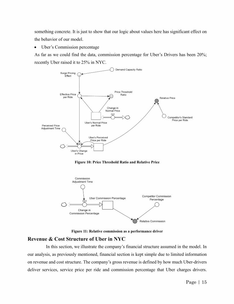
Page | 15
something concrete. It is just to show that our logic about values here has significant effect on
the behavior of our model.
• Uber’s Commission percentage
As far as we could find the data, commission percentage for Uber’s Drivers has been 20%;
recently Uber raised it to 25% in NYC.
Figure 10: Price Threshold Ratio and Relative Price
Figure 11: Relative commission as a performance driver
Revenue & Cost Structure of Uber in NYC
In this section, we illustrate the company’s financial structure assumed in the model. In
our analysis, as previously mentioned, financial section is kept simple due to limited information
on revenue and cost structure. The company’s gross revenue is defined by how much Uber-drivers
deliver services, service price per ride and commission percentage that Uber charges drivers.
Page | 16
Though, this measurement is rather an aggregated measurement of what’s done in reality, we tried
to capture the company’s revenue structure briefly. Cost structure is intentionally limited to bonus
spending due to unavailability of financial data and to avoid unnecessary effect on system behavior
at this point of research.
System Boundary
In this case study, the boundary of the system or scope of our analysis is set to an area of New York
City in terms of geographical boundary and data we have referenced. We consider that deciding
system boundary of the analysis is crucial in model development in the sense that it can either
improves or limits the capability of an explanatory model. One of the reasons why we set the
system in NYC is that the area is highly competitive and reference data were relatively easy to
find. Therefore, it serves as a good representation for our group project.
Limitations in the model
Qualitative researches have numerous advantages and strength when they are properly conducted.
Before we move into the behavior analysis of the model, we briefly mention a major limitation
that our model structure brings into effect.
One of the major constraints is a lack of feedback loop from financial part of the model.
As seen above, this is due to a lack of sufficient information about the company’s financial results.
Consequently, we have decided to focus more on the dynamics of customer and driver acquisition
of the business. To be more specific, gross monthly revenue is calculated, yet there is not a single
causal relationship with other parts of the model except bonus spending, leaving out possible
constraints of financial resources. In reality, however, strategic decisions and policies in
organizations are primarily affected by its financial capability. It should be noted that the behavior
which the current model produces has this kind of limitations behind it.
Insights from Model Analysis and Discussion
Behavior of the model: Default Case
We are now in the position to analyze behavior of the model in default case scenario. As we stated
in the introduction, Uber has been growing its business operation rapidly both internally and
externally. Specifically, our reference mode for active Uber-drivers is at exponential growth as
Page | 17
shown in Figure 4 (by cities). Time = 0 corresponds to the time when Uber began its first ride-
hailing service in NYC.
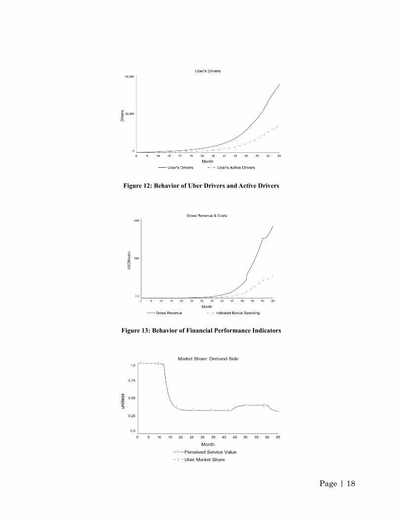
Figure 12 shows our comparative simulation result of Uber’s Drivers and active drivers.
Empowered by the reinforcing loops of word of mouth both in supply and demand side, the number
of drivers increases exponentially.
As a result of such business expansion, the model shows that monthly gross revenue
continues to grow at increasing rate. Behaviors of gross revenue and bonus spending are shown in
Figure 13. Uber’s cost structure in NYC, which consists only of bonus spending in the current
model is correspondingly increasing.
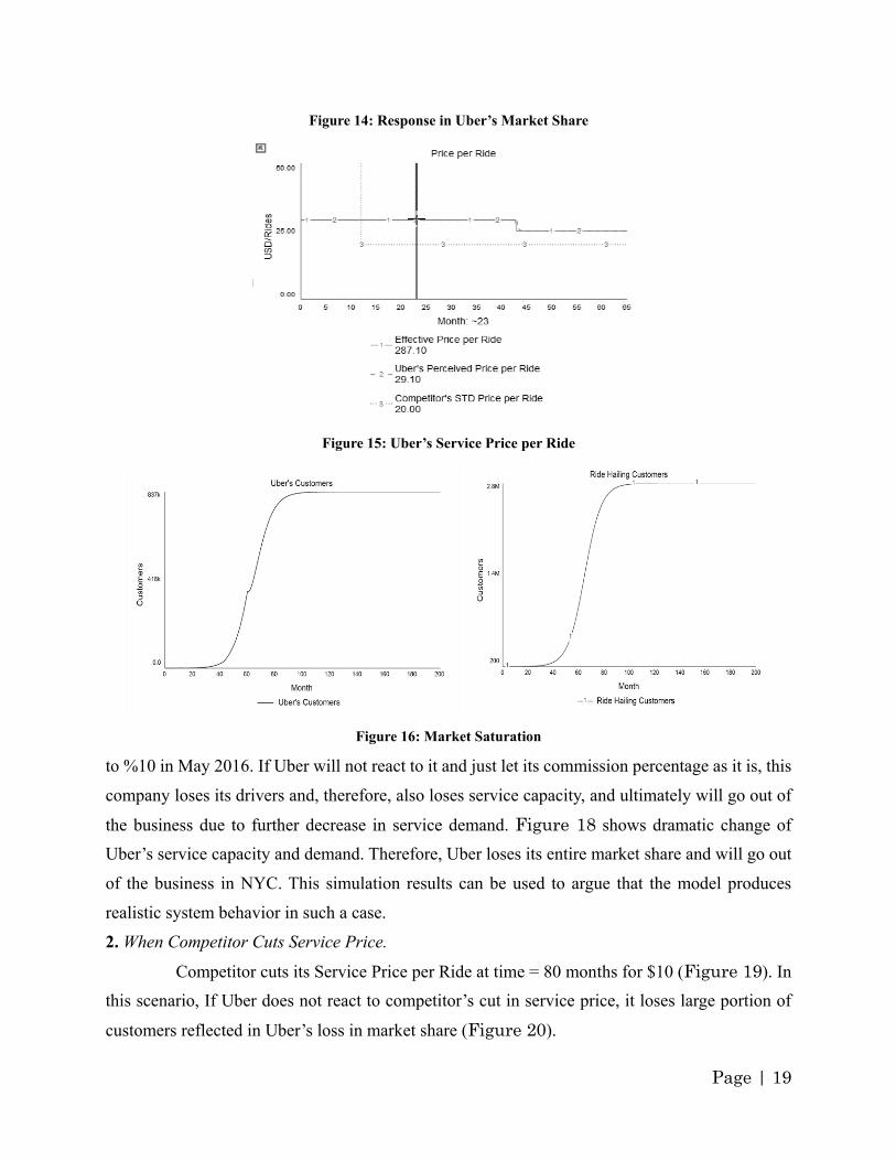
Figure 14 shows behavior of Uber’s market share in response to the entrance of its
main competitor, Gett, to NYC at time = 10 months.6. Initially, there was no ride-hailing service
competitor in NYC. Over time the competitor gradually gain market share until it reaches its steady
point. Then at time = 45 months, Uber cuts its service price by 15 %.7 As a result, Uber regain its
market share. Moreover, at time = 60 months, one of the competitors, Lyft reduces its pickup time
from 6 to 3 minutes.8 The loss in market share of Uber is a consequence of its competitor’s service
price change.
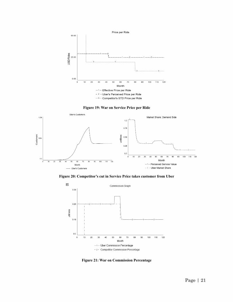
Limits to growth
So far, as the model is simulated in default scenario, the number of Uber’s customers could
continue to grow since the industry itself is expanding, supported by two reinforcing loops of word
of mouth. However, when the model is run until 200 months, it reaches a peak and the market
seems to saturate. This is certainly a result of limited capacity in the number of drivers and service
users in NYC. A specific value does not have significance itself. Rather, system structure which
produces certain behavior should be focused.
Scenario Analysis
1. Change in Commission Percentage
In the scenario 1, competitor cuts its commission from 20% to 10% at time = 60 months.
This happened in reality; Gett, one of Uber’s main competitor in NYC, reduced its commission
6 Uber’s competitor, Gett, launched operation in NYC in June 2012. (Mashable, 2012) 7 This change in Uber’s price is based on real case in Golson (2016)
8 “Since May 2016, Lyft has halved its average waiting time for a ride in NYC” (Wieczner, 2016).
Page | 18
Figure 12: Behavior of Uber Drivers and Active Drivers
Figure 13: Behavior of Financial Performance Indicators
Page | 19
Figure 14: Response in Uber’s Market Share
Figure 15: Uber’s Service Price per Ride
Figure 16: Market Saturation
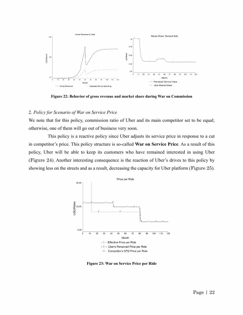
to %10 in May 2016. If Uber will not react to it and just let its commission percentage as it is, this
company loses its drivers and, therefore, also loses service capacity, and ultimately will go out of
the business due to further decrease in service demand. Figure 18 shows dramatic change of
Uber’s service capacity and demand. Therefore, Uber loses its entire market share and will go out
of the business in NYC. This simulation results can be used to argue that the model produces
realistic system behavior in such a case.
2. When Competitor Cuts Service Price.
Competitor cuts its Service Price per Ride at time = 80 months for $10 (Figure 19). In
this scenario, If Uber does not react to competitor’s cut in service price, it loses large portion of
customers reflected in Uber’s loss in market share (Figure 20).
Page | 20
Figure 17: Change in Commission Percentage
Figure 18: Uber’s loss of service capacity and market share
Policy Analysis
In this section, policies for each scenario case is presented and explained:
1. Policy for Scenario of War on Commission
Suppose that we introduce a policy where Uber adjusts “commission percentage” in response to a
change in competitor’s commission. In scenario 1, at time = 60 months, as competitor cuts its
commission from 20% to 10%, Uber perceives such move in competitor and adjusts its
commission with a small delay.
Page | 21
Figure 19: War on Service Price per Ride
Figure 20: Competitor’s cut in Service Price takes customer from Uber
Figure 21: War on Commission Percentage
Page | 22
Figure 22: Behavior of gross revenue and market share during War on Commission
2. Policy for Scenario of War on Service Price
We note that for this policy, commission ratio of Uber and its main competitor set to be equal;
otherwise, one of them will go out of business very soon.
This policy is a reactive policy since Uber adjusts its service price in response to a cut
in competitor’s price. This policy structure is so-called War on Service Price. As a result of this
policy, Uber will be able to keep its customers who have remained interested in using Uber
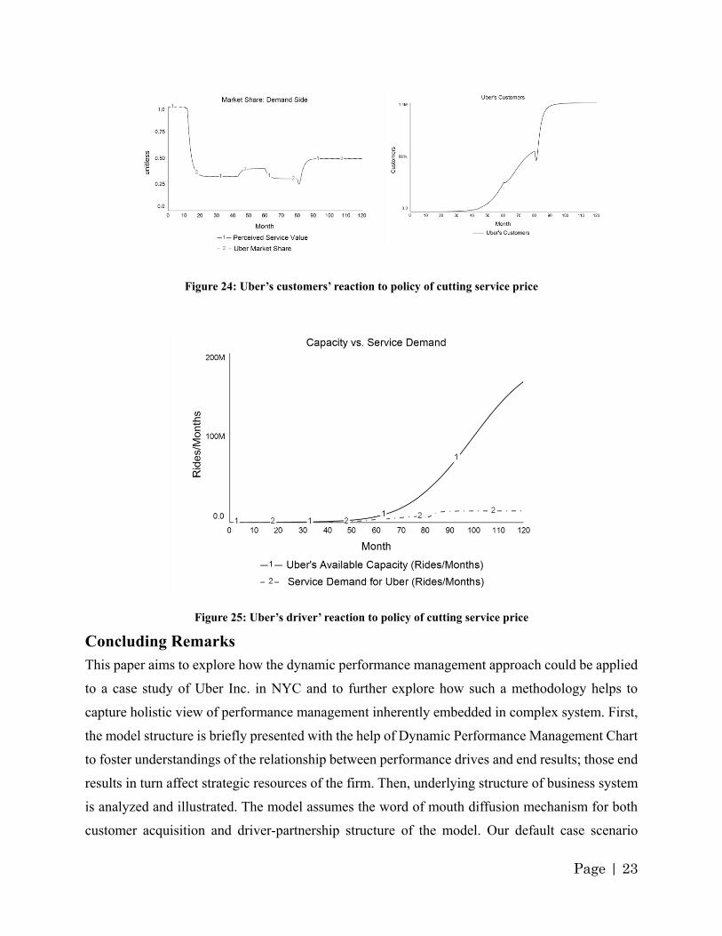
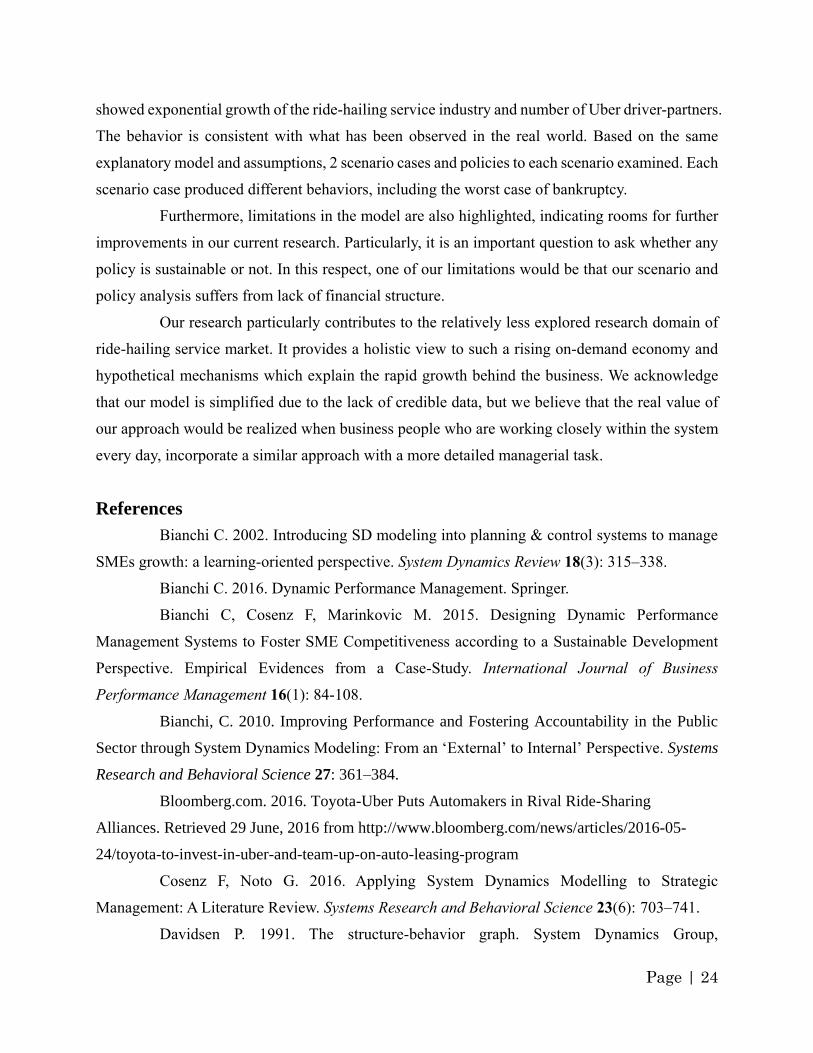
(Figure 24). Another interesting consequence is the reaction of Uber’s drives to this policy by
showing less on the streets and as a result, decreasing the capacity for Uber platform (Figure 25).
Figure 23: War on Service Price per Ride
Page | 23
Figure 24: Uber’s customers’ reaction to policy of cutting service price
Figure 25: Uber’s driver’ reaction to policy of cutting service price
Concluding Remarks
This paper aims to explore how the dynamic performance management approach could be applied
to a case study of Uber Inc. in NYC and to further explore how such a methodology helps to
capture holistic view of performance management inherently embedded in complex system. First,
the model structure is briefly presented with the help of Dynamic Performance Management Chart
to foster understandings of the relationship between performance drives and end results; those end
results in turn affect strategic resources of the firm. Then, underlying structure of business system
is analyzed and illustrated. The model assumes the word of mouth diffusion mechanism for both
customer acquisition and driver-partnership structure of the model. Our default case scenario
Page | 24
showed exponential growth of the ride-hailing service industry and number of Uber driver-partners.
The behavior is consistent with what has been observed in the real world. Based on the same
explanatory model and assumptions, 2 scenario cases and policies to each scenario examined. Each
scenario case produced different behaviors, including the worst case of bankruptcy.
Furthermore, limitations in the model are also highlighted, indicating rooms for further
improvements in our current research. Particularly, it is an important question to ask whether any
policy is sustainable or not. In this respect, one of our limitations would be that our scenario and
policy analysis suffers from lack of financial structure.
Our research particularly contributes to the relatively less explored research domain of
ride-hailing service market. It provides a holistic view to such a rising on-demand economy and
hypothetical mechanisms which explain the rapid growth behind the business. We acknowledge
that our model is simplified due to the lack of credible data, but we believe that the real value of
our approach would be realized when business people who are working closely within the system
every day, incorporate a similar approach with a more detailed managerial task.
References
Bianchi C. 2002. Introducing SD modeling into planning & control systems to manage
SMEs growth: a learning-oriented perspective. System Dynamics Review 18(3): 315–338.
Bianchi C. 2016. Dynamic Performance Management. Springer.
Bianchi C, Cosenz F, Marinkovic M. 2015. Designing Dynamic Performance
Management Systems to Foster SME Competitiveness according to a Sustainable Development
Perspective. Empirical Evidences from a Case-Study. International Journal of Business
Performance Management 16(1): 84-108.
Bianchi, C. 2010. Improving Performance and Fostering Accountability in the Public
Sector through System Dynamics Modeling: From an ‘External’ to Internal’ Perspective. Systems
Research and Behavioral Science 27: 361–384.
Bloomberg.com. 2016. Toyota-Uber Puts Automakers in Rival Ride-Sharing
Alliances. Retrieved 29 June, 2016 from http://www.bloomberg.com/news/articles/2016-05-
24/toyota-to-invest-in-uber-and-team-up-on-auto-leasing-program
Cosenz F, Noto G. 2016. Applying System Dynamics Modelling to Strategic
Management: A Literature Review. Systems Research and Behavioral Science 23(6): 703–741.
Davidsen P. 1991. The structure-behavior graph. System Dynamics Group,
Page | 25
Massachusetts Institute of Technology, Cambridge, MA.
Davidsen P. 1996. Educational features of the system dynamics approach to modeling
and simulation. Journal of Structural Learning 12(4): 269–290.
De Geus A. 1997. The Living Company. Habits for Survival in a Turbulent Business
Environment: Harvard Business School Press.
Fitzpatrick, A. (2012). This App Will Revolutionize the NYC Taxi Experience.
Retrieved 10 June, 2016, from Available at: http://mashable.com/2012/06/07/gettaxi/
Forbes.com. (2016). Uber Raises UberX Commission To 25 Percent In Five More
Markets. Retrieved 29 June, 2016, from http://www.forbes.com/sites/ellenhuet/2015/09/11/uber-
raises-uberx-commission-to-25-percent-in-five-more-markets/
Forrester JW. 1961. Industrial Dynamics. Cambridge, MA: MIT Press.
Ghaffarzadegan N, Lyneis J, Richardson GP. 2011. How small system dynamics models
can help the public policy process. System Dynamics Review 27(1): 22–44.
Golson J. 2016. Uber is slashing prices in New York City. Retrieved 29 June, 2016,
from http://www.theverge.com/2016/1/28/10864516/uber-cutting-uberx-rates-new-york-city
Hall J, Krueger A. 2015. An Analysis of the Labor Market for Uber's Driver-Partners
in the United States. Uber Technologies. Available from
https://irs.princeton.edu/sites/irs/files/An%20Analysis%20of%20the%20Labor%20Market%20fo
r%20Uber’s%20Driver-Partners%20in%20the%20United%20States%20587.pdf
Hall J, Kendrick C, Nosko C. 2015. The Effects of Uber's Surge Pricing: A Case
Study. Available from
http://faculty.chicagobooth.edu/chris.nosko/research/effects_of_uber's_surge_pricing.pdf
Isidore C. 2016. Union to represent 35,000 Uber drivers in New York City, but with
limits. Retrieved 29 June, 2016, from http://money.cnn.com/2016/05/11/news/companies/uber-
new-york-city-union/
Kaplan R. Norton D. 1996. The Balanced Scorecard: Translating Strategy into Action.
Boston: Harvard Business School Press.
Kulp P. 2016. Uber knows you're more likely to pay surge prices when your phone is
dying. Retrieved 30 June, 2016, from http://mashable.com/2016/05/21/uber-phone-batteries-
surge-pricing/
Linard K. Dvorsky L. 2001. People - not human resources: the system dynamics of
human capital accounting. Operations Research Society Conference, University of Bath, Bath.
Page | 26
Linard K, Fleming C, Dvorsky L. 2002. System Dynamics as the Link between
Corporate Vision and Key Performance Indicators. In Proceedings of the 20th System Dynamics
International Conference. Palermo, Italy.
Moon Y. 2015. Uber: Changing the Way the World Moves. Harvard Business School
Case, 316-101.
Morecroft J. 2007. Strategic modeling and business dynamics. Chichester: Wiley.
Neely A. 1999. The performance management revolution: why now and what next?
International Journal of Operations & Production Management 19(2): 205–228.
Neely A, Richards H, Mills J, Platts K. Bourne M. 1997. Designing performance
measures: a structured approach. International Journal of Operations & Production Management
17(11): 1131–52.
NYC Taxi & Limousine Commission, (2014). Taxicab Fact Book. New York City.
Otley D. 1999. Performance management: a framework for management control systems
research. Management Accounting Research 10(4): 363–382.
Richardson GP, Pugh AI. 1981. Introduction to system dynamics modeling with
DYNAMO. Productivity Press, New York.
Ridesharingdriver.com. (2016). Retrieved 29 June, 2016, from
http://www.ridesharingdriver.com/how-much-does-uber-cost-uber-fare-estimator/
Sloper P., Linard K. Paterson D. 1999. Towards a dynamic feedback framework for
public sector performance management. In Proceedings of the 17th International System Dynamics
Conference. Wellington, NZ.
Sterman JD. 2000. Business Dynamics: Systems Thinking and Modeling for a Complex
World. Irwin/McGraw-Hill, Boston.
Wieczner, J. (2016). Lyft Is Growing at a Crazy Pace in New York and San Francisco.
Retrieved 29 June, 2016, from http://fortune.com/2016/03/08/lyft-vs-uber-new-york/
Page | 27
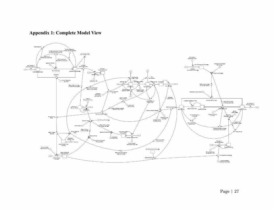
Appendix 1: Complete Model View
Page | 28
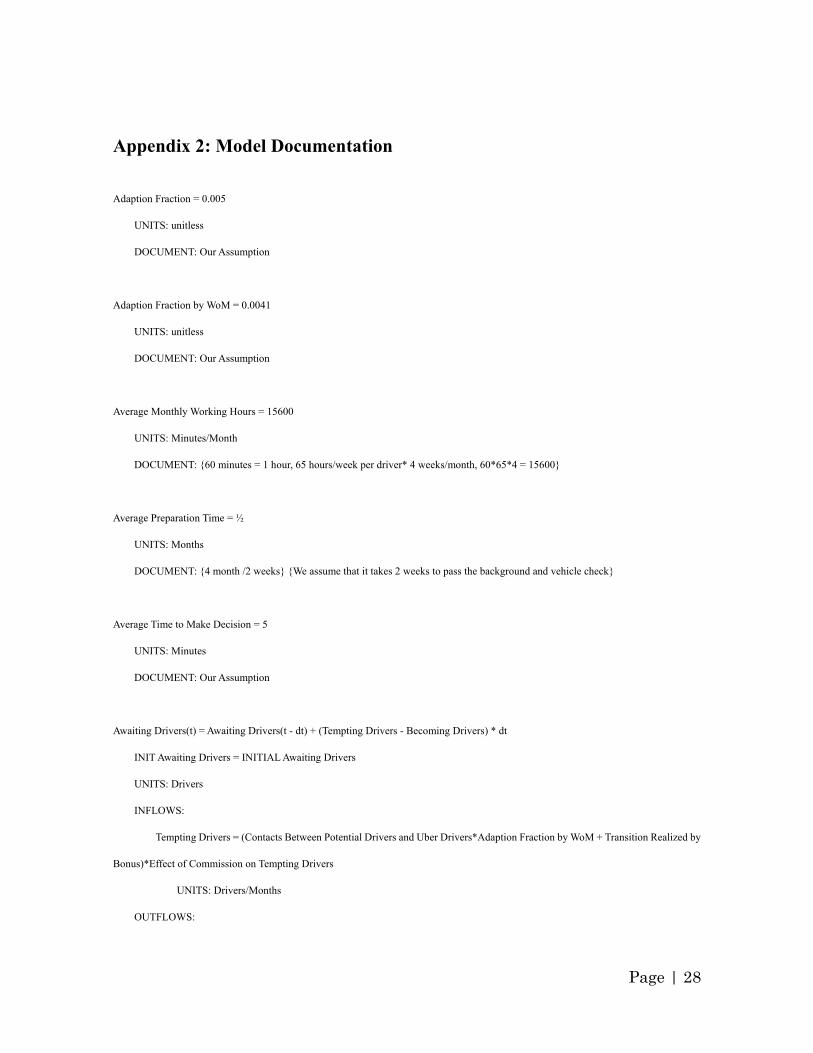
Appendix 2: Model Documentation
Adaption Fraction = 0.005
UNITS: unitless
DOCUMENT: Our Assumption
Adaption Fraction by WoM = 0.0041
UNITS: unitless
DOCUMENT: Our Assumption
Average Monthly Working Hours = 15600
UNITS: Minutes/Month
DOCUMENT: {60 minutes = 1 hour, 65 hours/week per driver* 4 weeks/month, 60*65*4 = 15600}
Average Preparation Time = ½
UNITS: Months
DOCUMENT: {4 month /2 weeks} {We assume that it takes 2 weeks to pass the background and vehicle check}
Average Time to Make Decision = 5
UNITS: Minutes
DOCUMENT: Our Assumption
Awaiting Drivers(t) = Awaiting Drivers(t - dt) + (Tempting Drivers - Becoming Drivers) * dt
INIT Awaiting Drivers = INITIAL Awaiting Drivers
UNITS: Drivers
INFLOWS:
Tempting Drivers = (Contacts Between Potential Drivers and Uber Drivers*Adaption Fraction by WoM + Transition Realized by
Bonus)*Effect of Commission on Tempting Drivers
UNITS: Drivers/Months
OUTFLOWS:
Page | 29
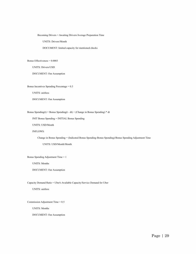
Becoming Drivers = Awaiting Drivers/Average Preparation Time
UNITS: Drivers/Month
DOCUMENT: limited capacity for mentioned checks
Bonus Effectiveness = 0.0003
UNITS: Drivers/USD
DOCUMENT: Our Assumption
Bonus Incentives Spending Percentage = 0.3
UNITS: unitless
DOCUMENT: Our Assumption
Bonus Spending(t) = Bonus Spending(t - dt) + (Change in Bonus Spending) * dt
INIT Bonus Spending = INITIAL Bonus Spending
UNITS: USD/Month
INFLOWS:
Change in Bonus Spending = (Indicated Bonus Spending-Bonus Spending)/Bonus Spending Adjustment Time
UNITS: USD/Month/Month
Bonus Spending Adjustment Time = 1
UNITS: Months
DOCUMENT: Our Assumption
Capacity Demand Ratio = Uber's Available Capacity/Service Demand for Uber
UNITS: unitless
Commission Adjustment Time = 0.5
UNITS: Months
DOCUMENT: Our Assumption
Page | 30
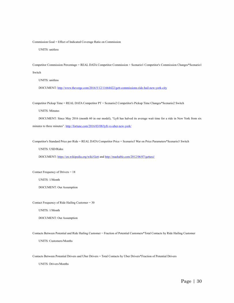
Commission Goal = Effect of Indicated Coverage Ratio on Commission
UNITS: unitless
Competitor Commission Percentage = REAL DATA Competitor Commission + Scenario1 Competitor's Commission Changes*Scenario1
Switch
UNITS: unitless
DOCUMENT: http://www.theverge.com/2016/5/12/11664422/gett-commissions-ride-hail-new-york-city
Competitor Pickup Time = REAL DATA Competitor PT + Scenario2 Competitor's Pickup Time Changes*Scenario2 Switch
UNITS: Minutes
DOCUMENT: Since May 2016 (month 60 in our model), “Lyft has halved its average wait time for a ride in New York from six
minutes to three minutes”. http://fortune.com/2016/03/08/lyft-vs-uber-new-york/
Competitor's Standard Price per Ride = REAL DATA Competitor Price + Scenario3 War on Price Parameters*Scenario3 Switch
UNITS: USD/Rides
DOCUMENT: https://en.wikipedia.org/wiki/Gett and http://mashable.com/2012/06/07/gettaxi/
Contact Frequency of Drivers = 18
UNITS: 1/Month
DOCUMENT: Our Assumption
Contact Frequency of Ride Hailing Customer = 30
UNITS: 1/Month
DOCUMENT: Our Assumption
Contacts Between Potential and Ride Hailing Customer = Fraction of Potential Customers*Total Contacts by Ride Hailing Customer
UNITS: Customers/Months
Contacts Between Potential Drivers and Uber Drivers = Total Contacts by Uber Drivers*Fraction of Potential Drivers
UNITS: Drivers/Months
Page | 31
Demand Capacity Ratio = Service Demand for Uber/Uber's Available Capacity
UNITS: unitless
Effect of Commission on Drivers Attrition = GRAPH(Relative Commission)
(0.000, 0.1), (0.250, 0.3), (0.500, 0.4), (0.750, 0.6), (1.000, 1.0), (1.250, 50.0), (1.500,
100.0), (1.750, 150.0), (2.000, 200.0), (2.250, 250.0), (2.500, 300.0), (2.750, 400.0),
(3.000, 500.0)
UNITS: unitless
DOCUMENT: The logic here is that as competitor offers less commissions (more
gain for Drivers), more and more drivers leave Uber and join its competitor.
Figure A1: Effect of Commission on Drivers Attrition
Effect of Commission on Tempting Drivers = GRAPH(Relative Commission)
(0.000, 2.000), (0.200, 2.000), (0.400, 1.930), (0.600, 1.825), (0.800, 1.572), (1.000,
1.000), (1.200, 0.611), (1.400, 0.419), (1.600, 0.288), (1.800, 0.148), (2.000, 0.070)
UNITS: unitless
DOCUMENT: The logic here is that as competitor offers less commissions (more
gain for Drivers), it becomes more difficult to tempt drivers to join Uber.
Figure A2: Effect of Commission on Tempting Drivers
Effect of Demand Capacity Ratio on Pickup Time = GRAPH(Demand Capacity Ratio)
(1.000, 1.00), (1.100, 1.10), (1.200, 1.17), (1.300, 1.24), (1.400, 1.40), (1.500, 1.66), (1.600, 2.14), (1.700, 2.88), (1.800, 4.25), (1.900,
6.65), (2.000, 10.00)
UNITS: unitless
DOCUMENT: An assumption behind this effect is that when service demand becomes (for example, twice as) higher than service
delivery capacity of Uber, Effective Pickup Time becomes nearly ten times longer than normal time. In other words, having twice as service
Page | 32
demand than service capacity does not simply mean that Uber’s pickup time becomes twice of normal times. In fact, we assumed the effect
would be much stronger until it hits certain threshold9. Our reasoning is as follows: When the service demand for Uber at a specific period
is twice as many as what the company can deliver, each Uber driver in NYC has two
people waiting for a ride at the same time. But some of the drivers need to refill the
gas or even they may get into traffic jam, etc. Therefore, the effect should be
increasingly stronger as Demand-Capacity ratio increases.
Why the maximum is the specific value of 10? Because this is the period between the
moment a customer hails a ride and the driver arrives. In NYC, considering the number
of available Uber driver, we assume that it will not exceed Uber's MIN Pickup Time
(= 3 minutes) * Max value of the Effect (= 10) = 30 minutes.10
Figure A3: Effect of Demand Capacity Ratio on Pickup Time
Effect of Indicated Coverage Ratio on Commission = GRAPH(Indicated Capacity Demand Ratio)
(0.000, 0.2000), (2.000, 0.0100)
UNITS: unitless
DOCUMENT: Our Assumption
Effect of Pickup Time on Service Value = GRAPH(Relative Pickup Time)
(0.000, 1.000), (0.200, 0.983), (0.400, 0.930), (0.600, 0.843), (0.800, 0.677), (1.000,
0.500), (1.200, 0.271), (1.400, 0.157), (1.600, 0.092), (1.800, 0.039), (2.000, 0.022)
UNITS: unitless
INPUT = Relative Waiting Time
Figure A4: Effect of Pickup Time on Service Value
9 Specifically, the maximum value is set to be 10.
10 For example, Uber car hailing service can be considered as a super-efficient version of ambulance in a sense that many available cars
are ready at a specific moment in NYC.
Page | 33
DOCUMENT: The assumption made behind this structure is that the longer Uber drivers make their customers wait, the more they
lose market share (to its competitors such as Gett, Lyft, Yellow cab). The degree of the effect is subjective since, on the shadow of lack of
information, we have not conducted regression analysis whatsoever. However, the curve of the graphical function is determined by our
logics based on our mental model. The horizontal line in the graph means that there will be no effect if “Relative Pickup time” is 1.
Effect of Price on Service Value = GRAPH(Relative Price)
(0.000, 1.000), (0.200, 0.983), (0.400, 0.930), (0.600, 0.843), (0.800, 0.677), (1.000,
0.500), (1.200, 0.271), (1.400, 0.157), (1.600, 0.092), (1.800, 0.039), (2.000, 0.022)
UNITS: unitless
DOCUMENT: Our Assumption
Figure A5: Effect of Price on Service Value
Effect of Price Threshold Ratio on Closing App = (Price Threshold Ratio/10) - 0.1
UNITS: unitless
DOCUMENT:
Figure A6: Effect of Price Threshold Ratio on Closing App
Threshold / 10 - 0.1 =
1 0.1 0.1 0
2 0.2 0.1 0.1
3 0.3 0.1 0.2
4 0.4 0.1 0.3
5 0.5 0.1 0.4
6 0.6 0.1 0.5
7 0.7 0.1 0.6
8 0.8 0.1 0.7
9 0.9 0.1 0.8
9 0.9 0.1 0.8
10 1 0.1 0.9
Page | 34
Effect of Price Threshold Ratio on Active Drivers = GRAPH(Price Threshold Ratio {We assume that in normal situation, price ratio of 1
leads to 40% of drivers availability})
(0.00, 0.000), (1.00, 0.400), (2.00, 0.502), (3.00, 0.590), (4.00, 0.664), (5.00, 0.721), (6.00, 0.790), (7.00, 0.834), (8.00, 0.882), (9.00, 0.921),
(10.00, 0.978)
UNITS: unitless
DOCUMENT: This effect is used to describe the change in active Uber drivers
when service price increase and becomes higher than normal rates. When Uber drivers
see service rate is surging, more and more drivers start turning on their car engines and
become involved actively. This concept of rise in service capacity is observed in real
case study. A case study of Hall, Kendrick and Nosko (2015) shows that the service
capacity can get to be 150% higher than normal times during surge period in the event
of sold-out musical concert in NYC. {We assume that in normal situation, price ratio
of 1 leads to 40% of drivers’ availability}
Figure A7: Effect of Threshold Ratio on Active Drivers
Effect of Service Value on Customer Acquisition = Perceived Service Value
UNITS: unitless
DOCUMENT: This variable is an intermediate one and it is equal to Perceived Service Value.
Effective Price per Ride = Uber's Normal Price per Ride*Surge Pricing Effect
UNITS: USD/Rides
Fraction of Potential Customers = Potential Customers/Total Ridership
UNITS: unitless
Fraction of Potential Drivers = Potential Drivers/Total Drivers
UNITS: unitless
Fraction of Uber's Active Drivers = Effect of Price Threshold Ratio on Drivers
UNITS: unitless
Page | 35
Gross Revenue = Uber Commission Percentage*Giving a Ride*Uber's Perceived Price per Ride
UNITS: USD/Month
Indicated Bonus Spending = Gross Revenue*Bonus Incentives Spending Percentage
UNITS: USD/Month
Indicated Capacity Demand Ratio = Policy4 Desired Capacity Demand Ratio - Capacity Demand Ratio
UNITS: unitless
Indicated Uber's Customers = Ride Hailing Customers*Effect of Service Value on Customer Acquisition
UNITS: Customers
INITIAL Awaiting Drivers = 0
UNITS: Drivers
INITIAL Bonus Spending = 10*26850 {10 Bonus * Average price of new passenger cars sold and leased in 2010}
UNITS: USD/Month
DOCUMENT: Average price of new passenger cars sold and leased, in 2010: 26850 USD
http://www.statista.com/statistics/183745/average-price-of-us-new-and-used-vehicle-sales-and-leases-since-1990/
INITIAL On Decision = 1
UNITS: Rides
INITIAL On Service = 0
UNITS: Rides
INITIAL POTENTIAL DRIVERS = 51398 + 1400000
UNITS: Drivers
DOCUMENT:
As of March 14, 2014, in New York City, there were 51,398 men and women licensed to drive medallion taxicabs.
There were 13,605 taxicab medallion licenses in existence, 368 of them having been auctioned by the City of New
Page | 36
York between November 2013 and February 2014.
https://en.wikipedia.org/wiki/Taxicabs_of_New_York_City
“According to the data, only 1.4 million households in the City out of the total 3.0 million owned a car”
(http://www.nycedc.com/blog-entry/new-yorkers-and-cars) Here, in our model, we ignore the fact that some car
owners may have more than one car!
INITIAL POTENTIAL Customers = 8175133/3
UNITS: Customers
DOCUMENT: 8175133 Initial population of NY City in 2010; we assume that just one third of them are potential customers
http://www1.nyc.gov/site/planning/data-maps/nyc-population/current-future-populations.page
INITIAL PT = 3
UNITS: Minutes
INITIAL Requested Rides = 1
UNITS: Rides
INITIAL Ride Hailing Customers = 200
UNITS: Customers
INITIAL Uber Commission Percentage = 0.2
UNITS: unitless
INITIAL Uber Drivers = 100
UNITS: Drivers
INITIAL UBER PRICE per RIDE = 29 {We assume it is equal to INITIAL Uber's Normal Price per Ride.}
UNITS: USD/Rides
INITIAL Uber's Normal Price per Ride = 29
Page | 37
UNITS: USD/Rides
DOCUMENT:
After Jan 2016:
$2.55 Base Fare + $0.35 per minutes *30 minutes + $1.75 per mile * 6.5 miles from Manhattan to East Brooklyn
= $24.425 25
(http://www.ridesharingdriver.com/how-much-does-uber-cost-uber-fare-estimator/ and http://uberestimate.com/prices/New-
York-City/ )
Before Jan 2016:
$3.00 Base Fare + $0.40 per minutes *30 minutes + $2.15 per mile * 6.5 miles from Manhattan to East Brooklyn
= $28.975 29
“Uber is slashing prices in New York City The base fare on UberX will go from $3 to $2.55, with the per mile rate going from
$2.15 to $1.75. The per minute rate will go from $0.40 to $0.35. UberXL will see drops of similar levels.”
(http://www.theverge.com/2016/1/28/10864516/uber-cutting-uberx-rates-new-york-city)
Matched Rides(t) = Matched Rides(t - dt) + (Requesting a Ride - Free Cancellation - Ride Arriving) * dt
INIT Matched Rides = INITIAL Requested Rides
UNITS: Rides
INFLOWS:
Requesting a Ride = On Decision/(Average Time to Make Decision/Time Converter)
UNITS: Rides/Months
OUTFLOWS:
Free Cancellation = SMTH1(Requesting a Ride*0.001, 5/Time Converter)*0 + 0
UNITS: Rides/Months
Ride Arriving = MIN(Matched Rides/(Uber's Average Pickup Time/Time Converter), Uber's Available Capacity)
UNITS: Rides/Months
Normal Regreters per Month = 5
UNITS: Customers/Month
Page | 38
On Decision(t) = On Decision(t - dt) + (Opening App - Requesting a Ride - Closing App Crazy Prices - Discarding Late Services) * dt
INIT On Decision = INITIAL On Decision
UNITS: Rides
INFLOWS:
Opening App = Service Demand for Uber
UNITS: Rides/Months
OUTFLOWS:
Requesting a Ride = On Decision/(Average Time to Make Decision/Time Converter)
UNITS: Rides/Months
Closing App Crazy Prices = Opening App*Effect of Price Threshold Ratio on Closing App
UNITS: Rides/Months
Discarding Late Services = IF (Uber's Effective Pickup Time > 60) THEN SMTH1((Opening App - Requesting a Ride), 1/30)
ELSE 0 {If effective waiting time exceeds 1Hours (= 60 minutes), customers cancel their rides (requests)}
UNITS: Rides/Months
On Service(t) = On Service(t - dt) + (Ride Arriving - Giving a Ride) * dt
INIT On Service = INITIAL On Service
UNITS: Rides
INFLOWS:
Ride Arriving = MIN(Matched Rides/(Uber's Average Pickup Time/Time Converter), Uber's Available Capacity)
UNITS: Rides/Months
OUTFLOWS:
Giving a Ride = On Service/(Standard Riding Time/Time Converter)
UNITS: Rides/Months
Perceived Price Adjustment Time = 1/4 {about a week}
UNITS: Months
Perceived Service Value(t) = Perceived Service Value(t - dt) + (Change in Perceived SV) * dt
INIT Perceived Service Value = Service Value
Page | 39
UNITS: unitless
INFLOWS:
Change in Perceived SV = (Service Value - Perceived Service Value)/Time to Change Perceives
UNITS: 1/month
Pickup Time Weight = 0.25
UNITS: unitless
Policy1 Switch = IF TIME > 80 THEN 1*0 ELSE 0 {0 = off, 1 = on} {Change 1*0 to 1 to activate this switch} {Tnis scenario is very
sensitive to time, if it is activated late, company will fail; here 80 is too much!}
UNITS: unitless
Policy2 Change in MIN Pickup Value = -1
UNITS: Minutes
Policy2 Switch = 0 {0 = off, 1 = on}
UNITS: unitless
Policy2 Time = 80 {month}
UNITS: Months
DOCUMENT: Timing of policy implementation has significant effect on the performance of the business; Test these values: Change
in MIN Waiting Time = -3; Policy2 Time = 1 vs 30
Policy3 Adjustment Time = 1/2 {half a month}
UNITS: Months
Policy3 Switch = IF TIME > 80 THEN 1*0 ELSE 0 {0 = off, 1 = on} {Change 1*0 to 1 to activate this switch}
UNITS: unitless
Policy4 Desired Capacity Demand Ratio = 3
UNITS: unitless
Page | 40
Policy4 Switch = IF TIME > 70 THEN 1*0 ELSE 0 {0 = off, 1 = on} {Change 1*0 to 1 to activate this switch}
UNITS: unitless
Potential Customers(t) = Potential Customers(t - dt) + (Net Change in Potential Customers + Regreters - New Customers) * dt
INIT Potential Customers = INITIAL POTENTIAL Customers
UNITS: Customers
DOCUMENT: An important assumption: We assume that the population of the NY City is constant during the 5 years period of
simulation.
INFLOWS:
Net Change in Potential Customers = 0
UNITS: Customers/Months
Regreters = Surge Pricing Effect*Normal Regreters per Month
UNITS: Customers/Months
OUTFLOWS:
New Customers = Contacts Between Potential and Ride Hailing Customer*Adaption Fraction
UNITS: Customers/Months
Potential Drivers(t) = Potential Drivers(t - dt) + (Drivers Leaving Uber + Net Change in Potential Drivers - Tempting Drivers) * dt
INIT Potential Drivers = INITIAL POTENTIAL DRIVERS
UNITS: Drivers
INFLOWS:
Drivers Leaving Uber = Standard Drivers Attrition*Effect of Commission on Drivers Attrition
UNITS: Drivers/Month
Net Change in Potential Drivers = 0
UNITS: Drivers/Months
OUTFLOWS:
Tempting Drivers = (Contacts Between Potential Drivers and Uber Drivers*Adaption Fraction by WoM + Transition Realized by
Bonus)*Effect of Commission on Tempting Drivers
UNITS: Drivers/Months
Page | 41
Price Threshold Ratio = SMTH1(Effective Price per Ride/Uber's Normal Price per Ride, DT, 1) {smoothing time = one DT}
UNITS: unitless
Price Weight = 0.75
UNITS: unitless
REAL DATA Competitor Commission = 10000 + STEP(-10000+0.2, 10) + STEP(-0.1, 60) {To make sure that before arrival of our first
competitor in March 2012 (Month 10), all of market share goes to Uber}
UNITS: unitless
REAL DATA Competitor Price = 10000 + STEP(-10000+20, 12) {To make sure that before arrival of our first competitor in March 2012
(Month 10), all of market share goes to Uber} {we assume Gett entered the NYC market with $20 per ride}
UNITS: USD/Rides
REAL DATA Competitor PT = 10000 + STEP(-10000+6, 10) + STEP(-3, 60) {To make sure that before arrival of our first competitor in
March 2012 (Month 10), all of market share goes to Uber}
UNITS: Minutes
DOCUMENT:
Since May 2016 (moth 60 in our model), Lyft has halved its average wait time for a ride in New York from six minutes
to three minutes, the spokesperson added by way of explaining the 500% ridership growth. Both Lyft and Uber have
also been aggressively slashing their prices in New York and other cities as they compete with each other to win
customers. http://fortune.com/2016/03/08/lyft-vs-uber-new-york/
REAL DATA Uber Commission = PULSE(0.05, 52, 0) {in September 2015, increased to 25%; September 2015 = Month 52 in our model}
UNITS: 1/month
REAL DATA Uber Price = PULSE(-4, 43, 0)
UNITS: USD/Rides/Month
DOCUMENT: in Jan. 2016, Uber slashed its prices by 15% in NYC and some other markets. Jan 2016 = Month 43 in our model.
Page | 42
Relative Commission = Uber Commission Percentage/Competitor Commission Percentage
UNITS: unitless
Relative Pickup Time = Uber's Perceived Pickup Time/Competitor Pickup Time
UNITS: unitless
Relative Price = Uber's Perceived Price per Ride/Competitor's Standard Price per Ride
UNITS: unitless
Reported Uber's Customers(t) = Reported Uber's Customers(t - dt) + (Change in UC) * dt
INIT Reported Uber's Customers = Indicated Uber's Customers
UNITS: Customers
INFLOWS:
Change in UC = (Indicated Uber's Customers-Reported Uber's Customers)/Reporting Time
UNITS: Customers/Months
Reporting Time = 1
UNITS: Months
Ride Hailing Customers(t) = Ride Hailing Customers(t - dt) + (New Customers - Regreters) * dt
INIT Ride Hailing Customers = INITIAL Ride Hailing Customers
UNITS: Customers
INFLOWS:
New Customers = Contacts Between Potential and Ride Hailing Customer*Adaption Fraction
UNITS: Customers/Months
OUTFLOWS:
Regreters = Surge Pricing Effect*Normal Regreters per Month
UNITS: Customers/Months
Scenario1 Competitor's Commission Changes = STEP(-0.09, 80) {Change in Value, Time in Month}
Page | 43
UNITS: unitless
Scenario1 Switch = IF TIME > 70 THEN 1*0 ELSE 0 {0 = off, 1 = on} {Change 1*0 to 1 to activate this switch}
UNITS: unitless
Scenario2 Competitor's Pickup Time Changes = STEP(-3, 100) {Change in Value, Time in Month}
UNITS: Minutes
Scenario2 Switch = 0 {0 = off, 1 = on}
UNITS: unitless
Scenario3 Switch = IF TIME > 80 THEN 1*0 ELSE 0 {0 = off, 1 = on} {Change 1*0 to 1 to activate this switch}
UNITS: unitless
Scenario3 War on Price Parameters = STEP(-10, 80) {Change in Value, Time in Month}
UNITS: USD/Rides
Service Demand for Uber = Reported Uber's Customers*Standard Rides Need per Customer
UNITS: Rides/Months
Service Value = Price Weight*Effect of Price on Service Value + Pickup Time Weight*Effect of Pickup Time on Service Value
UNITS: unitless
Shock Test Switch = 0 {0 = off, 1 = on}
UNITS: unitless
Shock Time = 23 {month}
UNITS: Months
Shock Value = 0.1 {The Pulse Value is very sensitive to DT. So, a tiny value of 0.1 will be divided by DT = 0.0001 which result in 100}
UNITS: Rides/Customers
Page | 44
Standard Driver per Ride = 1
UNITS: Drivers/Rides
Standard Drivers Attrition = 5
UNITS: Drivers/Month
Standard Rides Need per Customer = 10 + PULSE(Shock Value, Shock Time, 0)*Shock Test Switch
UNITS: Rides/Months/Customers
DOCUMENT: 10 rides per week, 4 weeks in a month {The Pulse Value is very sensitive to DT. So, a tiny value of 0.1 will be divided
by DT = 0.0001 which result in 100}
Standard Riding Time = 45 {0.75 hours = 45 minutes}
UNITS: Minutes
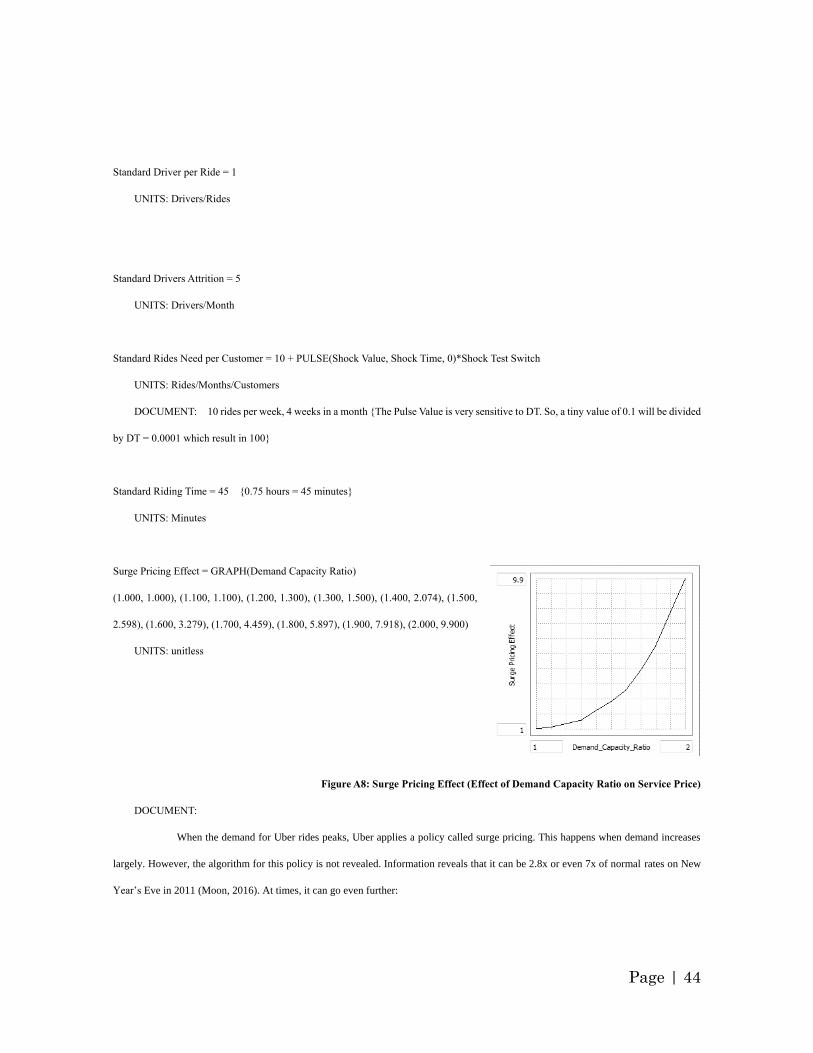
Surge Pricing Effect = GRAPH(Demand Capacity Ratio)
(1.000, 1.000), (1.100, 1.100), (1.200, 1.300), (1.300, 1.500), (1.400, 2.074), (1.500,
2.598), (1.600, 3.279), (1.700, 4.459), (1.800, 5.897), (1.900, 7.918), (2.000, 9.900)
UNITS: unitless
Figure A8: Surge Pricing Effect (Effect of Demand Capacity Ratio on Service Price)
DOCUMENT:
When the demand for Uber rides peaks, Uber applies a policy called surge pricing. This happens when demand increases
largely. However, the algorithm for this policy is not revealed. Information reveals that it can be 2.8x or even 7x of normal rates on New
Year’s Eve in 2011 (Moon, 2016). At times, it can go even further:
Page | 45
Surge pricing is one of Uber's most widely hated features. Just look at social media the day after any big holiday
and you'll see a flood of screenshots complaining of rates up to 9.9 times the company's normal price. (Kulp, 2016).
Based on this information, we assumed that company’s surging price algorithm features a quite steep slope when demand exceeds service
capacity as shown in the Figure A8. This effect lies in the center of interaction of supply and demand side of the model.
Time Converter = 43800
UNITS: Minutes/Month
Time to Adjust Perceived Pickup Time = 1/4 {1 weeks / 4 weeks in a month}
UNITS: Months
Time to Change Perceives = 1
UNITS: Months
Total Contacts by Ride Hailing Customer = Contact Frequency of Ride Hailing Customer*Ride Hailing Customers
UNITS: Customers/Months
Total Contacts by Uber Drivers = Uber's Drivers*Contact Frequency of Drivers
UNITS: Drivers/Months
Total Drivers = Potential Drivers + Uber's Drivers
UNITS: Drivers
Total Ridership = Potential Customers + Ride Hailing Customers
UNITS: Customers
Transition Realized by Bonus = Fraction of Potential Drivers*Bonus Spending*Bonus Effectiveness
UNITS: Drivers/Months
Page | 46
Uber Commission Percentage(t) = Uber Commission Percentage(t - dt) + (Change in Commission Percentage) * dt
INIT Uber Commission Percentage = INITIAL Uber Commission Percentage
UNITS: unitless
DOCUMENT:http://www.forbes.com/sites/ellenhuet/2015/09/11/uber-raises-uberx-commission-to-25-percent-in-five-more-markets/
INFLOWS:
Change in Commission Percentage = REAL DATA Uber Commission + Policy4 Switch*(Commission Goal-Uber Commission
Percentage)/Commission Adjustment Time +Policy1 Switch*War on Commission/Commission Adjustment Time
UNITS: 1/Month
Uber Market Share = Indicated Uber's Customers/Ride Hailing Customers
UNITS: unitless
Uber's Active Drivers = Uber's Drivers*Fraction of Uber's Active Drivers
UNITS: Drivers
Uber's Available Capacity = ((Uber's Active Drivers/Standard Driver per Ride)*Average Monthly Working Hours)/Standard Riding Time
UNITS: Rides/Months
Uber's Average Pickup Time = Uber's MIN Pickup Time*Effect of Demand Capacity Ratio on Pickup Time
UNITS: Minutes
Uber's Drivers(t) = Uber's Drivers(t - dt) + (Becoming Drivers - Drivers Leaving Uber) * dt
INIT Uber's Drivers = INITIAL Uber Drivers
UNITS: Drivers
INFLOWS:
Becoming Drivers = Awaiting Drivers/Average Preparation Time
UNITS: Drivers/Month
DOCUMENT: Later we may add more details: limited capacity for mentioned checks
OUTFLOWS:
Drivers Leaving Uber = Standard Drivers Attrition*Effect of Commission on Drivers Attrition
Page | 47
UNITS: Drivers/Month
Uber's Effective Pickup Time = (Matched Rides/Ride Arriving)*Time Converter
UNITS: Minutes
Uber's MIN Pickup Time = 3 + STEP(Policy2 Change in MIN Pickup Value, Policy2 Time)*Policy2 Switch
UNITS: Minutes
DOCUMENT: “Uber CEO explains why arrival time on the app is never accurate…. Kalanick said that the average wait time in major
cities for an ordered Uber is about 3 minutes.” (http://bgr.com/2016/01/04/uber-arrival-time-late/)
Uber's Normal Price per Ride(t) = Uber's Normal Price per Ride(t - dt) + (Change in Normal Price) * dt
INIT Uber's Normal Price per Ride = INITIAL Uber's Normal Price per Ride
UNITS: USD/Rides
INFLOWS:
Change in Normal Price = REAL DATA Uber Price + Policy3 Switch*(War on Price/Policy3 Adjustment Time)
UNITS: USD/Rides/Month
Uber's Perceived Pickup Time(t) = Uber's Perceived Pickup Time(t - dt) + (Change in Pickup Time) * dt
INIT Uber's Perceived Pickup Time = INITIAL PT
UNITS: Minutes
INFLOWS:
Change in Pickup Time = (Uber's Effective Pickup Time-Uber's Perceived Pickup Time)/Time to Adjust Perceived Pickup Time
UNITS: Minutes/Month
Uber's Perceived Price per Ride(t) = Uber's Perceived Price per Ride(t - dt) + (Uber's Change in Price) * dt
INIT Uber's Perceived Price per Ride = INITIAL UBER PRICE per RIDE
UNITS: USD/Rides
INFLOWS:
Uber's Change in Price = (Effective Price per Ride - Uber's Perceived Price per Ride)/Perceived Price Adjustment Time
UNITS: USD/Rides/Month
Page | 48
War on Commission = Competitor Commission Percentage - Uber Commission Percentage
UNITS: unitless
War on Price = Competitor's Standard Price per Ride - Uber's Normal Price per Ride
UNITS: USD/Rides
{The model has 139 variables. Stocks: 15; Flows: 21; Converters: 103; Constants: 47; Equations: 77; Graphicals: 8}