Int J Soc Robot (2010) 2: 79–94DOI 10.1007/s12369-009-0037-z

Probabilistic Autonomous Robot Navigation in DynamicEnvironments with Human Motion Prediction

Amalia F. Foka · Panos E. Trahanias

Accepted: 16 December 2009 / Published online: 6 January 2010© Springer Science & Business Media BV 2010

Abstract This paper considers the problem of autonomousrobot navigation in dynamic and congested environments.The predictive navigation paradigm is proposed where prob-abilistic planning is integrated with obstacle avoidancealong with future motion prediction of humans and/or otherobstacles. Predictive navigation is performed in a globalmanner with the use of a hierarchical Partially ObservableMarkov Decision Process (POMDP) that can be solved on-line at each time step and provides the actual actions therobot performs. Obstacle avoidance is performed within thepredictive navigation model with a novel approach by decid-ing paths to the goal position that are not obstructed by othermoving objects movement with the use of future motion pre-diction and by enabling the robot to increase or decrease itsspeed of movement or by performing detours. The robot isable to decide which obstacle avoidance behavior is optimalin each case within the unified navigation model employed.

Keywords Navigation · Obstacle avoidance · Motionprediction · Path planning · POMDPs

1 Introduction

For humans, the ability to navigate intentionally is eminent.For mobile robotic systems, however, navigation in dynamic

A.F. Foka (�)Department of Computer Engineering & Informatics, Universityof Patras, 26500 Patras, Greecee-mail: foka@ceid.upatras.gr

P.E. TrahaniasInstitute of Computer Science, Foundation for Researchand Technology—Hellas (FORTH), P.O. Box 1385, Heraklion,711 10 Crete, Greecee-mail: trahania@ics.forth.gr

real-world environments is an extremely complex and chal-lenging task. Such environments are characterized by theircomplex structure and the movement of humans and objectsin them. The robot has to avoid collision with obstacles andalso reach its goal position in a fast and optimal manner.

The problem of a robot navigating in a crowded environ-ment is treated so far mainly by incorporating separate co-operating modules for global path planning, local path plan-ning (obstacle avoidance) and localization. This paper uti-lizes a unified model that incorporates the modules for lo-calization, global and local motion planning. The employedmodel is a hierarchical POMDP specifically designed for au-tonomous robot navigation, termed as the Robot Navigation-HPOMDP (RN-HPOMDP), originally presented in [9]. TheRN-HPOMDP enables us to perform all aspects of nav-igation in a probabilistic and unified manner since thereis no intervention of any other external module. The RN-HPOMDP offers great advantages since probabilistic ap-proaches for localization and mapping have been widely em-ployed but this is not the case for robot motion planning.The modelling of the RN-HPOMDP is presented in [9] andin this paper its application under the predictive navigationparadigm is introduced.

Probabilistic planning is performed under the predictivenavigation paradigm in order to be able to simulate as best aspossible the human behavior for obstacle avoidance. Futuremotion prediction is an intrinsic behavior of humans. Whenhumans walk in an environment they perceive through theirvision the movement of other humans or other moving ob-jects. Humans use this information and attempt to estimatethe easiest, i.e. unblocked, and shortest path they should fol-low to reach their destination. This is in effect a predictivebehavior. It would be desirable for an autonomous robot todevelop a similar behavior. Future motion prediction allowsto obtain paths that are not only optimal in a time or distance

80 Int J Soc Robot (2010) 2: 79–94

traveled sense but it can also foresee situations where the ro-bot might get blocked and chooses new paths that avoid suchsituations.

The predictive navigation paradigm presented in this pa-per enables the robot to decide the best behavior for obsta-cle avoidance in each case. The robot can decide at any timestep to either change completely its path to its goal positionin order to follow an unblocked path, or perform a detour.The detour will be executed well before the robot gets tooclose to the obstacles and in addition the robot has foreseenthat after performing this detour it will be able to completeits path to the goal position without any other obstructions.Furthermore, the robot can also decide to change its speed ofmovement to a lower one to allow an obstacle to move awayfrom its motion path or bypass the obstacle by increasing itsspeed.

Obstacle avoidance in the proposed framework offersgreat advantages over standard methods present in [2, 3, 10,13, 18, 21, 23]. The main disadvantage of all these methodsis that they treat the problem locally. The local treatment ofthe problem directs the robot into executing globally subop-timal paths to its destination point. This is due to the factthat they stick on the initial planned path to the destinationpoint obtained by the global path planning module and donot replan no matter the changes that occur in the environ-ment.

Furthermore, obstacle avoidance in the proposed ap-proach is performed within the predictive navigation frame-work, i.e. it utilizes future motion prediction of humansand/or other objects to decide what is the best approach therobot should employ. In the proposed approach two kinds ofprediction are utilized: short-term and long-term. The short-term prediction refers to the one-step ahead prediction andthe long-term to the prediction of the final destination pointof the obstacle’s movement. One-step ahead prediction hasbeen previously utilized for obstacle avoidance in [5, 6, 12,17, 19, 20, 24, 25, 27, 28]. However, knowing an obstacle’scurrent position and its immediate next time-step position isnot indicative about the general obstacle behavior. In result,one-step ahead prediction can potentially assist the obstacleavoidance module locally but cannot be that effective whendeciding the final complete path the robot will execute toreach its destination position. For this reason, long-term pre-diction is employed that estimates the final destination pointof an obstacle’s motion trajectory. Recent methodologies forpredicting the whole path an obstacle is following have beenproposed in [1, 4, 16, 22, 26].

Finally, the robot can also avoid obstacles either by in-creasing its speed to bypass the obstacle or decreasing itsspeed to let the obstacle move away from the robot. Con-sequently, future motion prediction is also exploited to en-able the robot to decide if it should increase or decrease itsspeed to avoid an obstacle more effectively. Once more, this

feature is integrated into the global navigation model, theRN-HPOMDP.

Experimental results have shown the applicability of theproposed approach for predictive autonomous robot naviga-tion in dynamic environments where humans and movingobjects are avoided efficiently and the robot follows optimalpaths to reach its destination.

The remaining of this paper describes how predictivenavigation is achieved with the use of the RN-HPOMDPthat is outlined in Sect. 2. First, it is described how futuremotion prediction is obtained in Sect. 3 and how it is inte-grated to the global navigation model in Sect. 4. Following,the methodology used to enable the robot to avoid obstaclesby changing its speed of movement is presented in Sect. 5.Finally, the results and the conclusions of this work are pre-sented in Sects. 6, 7 and 8, respectively.

2 Partially Observable Markov Decision Processes

In this paper, we utilize a hierarchical representation ofPOMDPs specifically designed for autonomous robot nav-igation, the RN-HPOMDP as detailed in [9]. Here, the for-mulation of the RN-HPOMDP is presented for clarity rea-sons and the rest of this paper is concerned with its ap-plication to the predictive navigation problem. The RN-HPOMDP can efficiently model large real world environ-ments at a fine resolution and can be solved in real time. It isutilized as a unified framework for the autonomous robotnavigation problem, where no other external modules areused to drive the robot. In other words, the RN-HPOMDPintegrates the modules for localization, planning and obsta-cle avoidance. The RN-HPOMDP is solved on-line at eachtime step and decides the actual actions the robot performs.

2.1 POMDP Formulation for Robot Navigation

In the following we present a formulation of POMDPs forautonomous robot navigation in a unified framework. ThePOMDP decides the actions the robot should perform toreach its goal and also robustly tracks the robot’s locationin a probabilistic manner. In the problem considered in thispaper, we are interested in dynamic environments and hencethe POMDP also performs obstacle avoidance. All threefunctionalities are carried out without the intervention of anyother external module.

In our implementation the robot perceives the environ-ment by taking horizontal laser scans. In addition, an occu-pancy grid map (OGM) of the environment obtained at thedesired discretization is provided. The OGM is used to de-termine the set of possible states the robot might occupy.Laser measurements are used to obtain observations. In thefollowing, the elements of a POMDP, 〈S, A, T , R, Z, O〉,are instantiated for robot navigation as:

Int J Soc Robot (2010) 2: 79–94 81

Set of states, S : Each state in S corresponds to a discreteentry cell in the environment’s occupancy grid map (OGM)and an orientation angle of the robot with respect toa global reference system, i.e. each state s is a triplet(x, y, θ).

Set of actions, A: It consists of all possible rotation actionsfrom 0◦ to 360◦ termed as “action angles”.

Set of observations, Z : The observation set is the elementof the POMDP that assists in the localization of the robot,that is the belief update after an action has been executed.The set of observations is instantiated as the output of theiterative dual correspondence (IDC) algorithm of Lu andMilios [15] for scan matching.

Reward function, R: Since the proposed POMDP is used asa unified framework for robot navigation that will providethe actual actions the robot will perform and also carry outlocal obstacle avoidance for moving objects, the rewardfunction is updated at each time step. The reward func-tion is built and updated at each time step, according totwo reward grid maps (RGMs): a static and a dynamic asin [7]. The RGM is defined as a grid map of the environ-ment in analogy with the OGM. Each of the RGM cellscorresponds to a specific area of the environment with thesame discretization of the OGM, only that the value asso-ciated with each cell in the RGM represents the reward thatwill be assigned to the robot for ending up in a specific cell.The static RGM is built once by calculating the distance ofeach cell to the goal position and by incorporating informa-tion about cells belonging to static obstacles. The dynamicRGM is responsible for incorporating into the model in-formation about the current state of the environment, i.e.whether there are objects moving within it or other un-mapped objects. The detailed procedure for building andupdating the RGMs is given in Sect. 4.

Transition and observation functions, T and O: They areinitially defined according to the motion model of the robotand then they are learned as detailed in [9].

3 Motion Prediction

Motion prediction is utilized to obtain a more effective be-havior for obstacle avoidance. Two kinds of prediction areused: short-term and long-term prediction. Short-term pre-diction refers to the one-step ahead prediction of a human’sor an other object’s future position. Short-term predictionis obtained by a Polynomial Neural Network (PNN) that istrained with an evolutionary method as originally presentedin [7]. The PNN is trained once offline with motion data ob-tained and thus there is no computational overhead for short-term prediction. Furthermore, the results obtained from thePNN are significantly more accurate than any other simpler

prediction model. Long-term prediction refers to the predic-tion of the final destination point of a human’s or an otherobject’s motion trajectory.

3.1 Long-Term Prediction

Prediction methods known so far give satisfactory results forone-step ahead prediction. For the robot navigation task itwould be more useful to have many-steps ahead prediction.This would give the robot sufficient time and space to per-form the necessary manoeuvres to avoid obstacles and moreimportantly change its route towards its destination position.It is desirable for the robot to develop a behavior that willprefer routes that are not crowded and thus avoid ever get-ting stuck.

It is unlikely that any of the available standard predic-tion methods would give satisfactory results for many-stepsahead prediction, given the complexity of the movement be-havior. To achieve this, it is proposed to employ a long-termprediction mechanism. The long-term prediction refers tothe prediction of a human’s final destination position. It isplausible to assume that humans mostly do not just movearound but instead move purposively with the intention ofreaching a specific location. Our approach for performinglong-term prediction is based on the definition of the so-called “hot” points (HPs) in the environment, i.e. the pointswhere people would have interest in visiting them. For ex-ample, in an office environment desks, doors and chairsare objects that people have interest in reaching them andcould be defined as hot points of interest. In a museum,the points of interest can be defined as the various exhibitsthat are present. Moreover, other features of the environ-ment such as the entry points, passages, etc., can be de-fined as points of interest. Evidently, hot points of interestconvey semantic information about a workspace and hencecan only be defined with respect to the particular environ-ment.

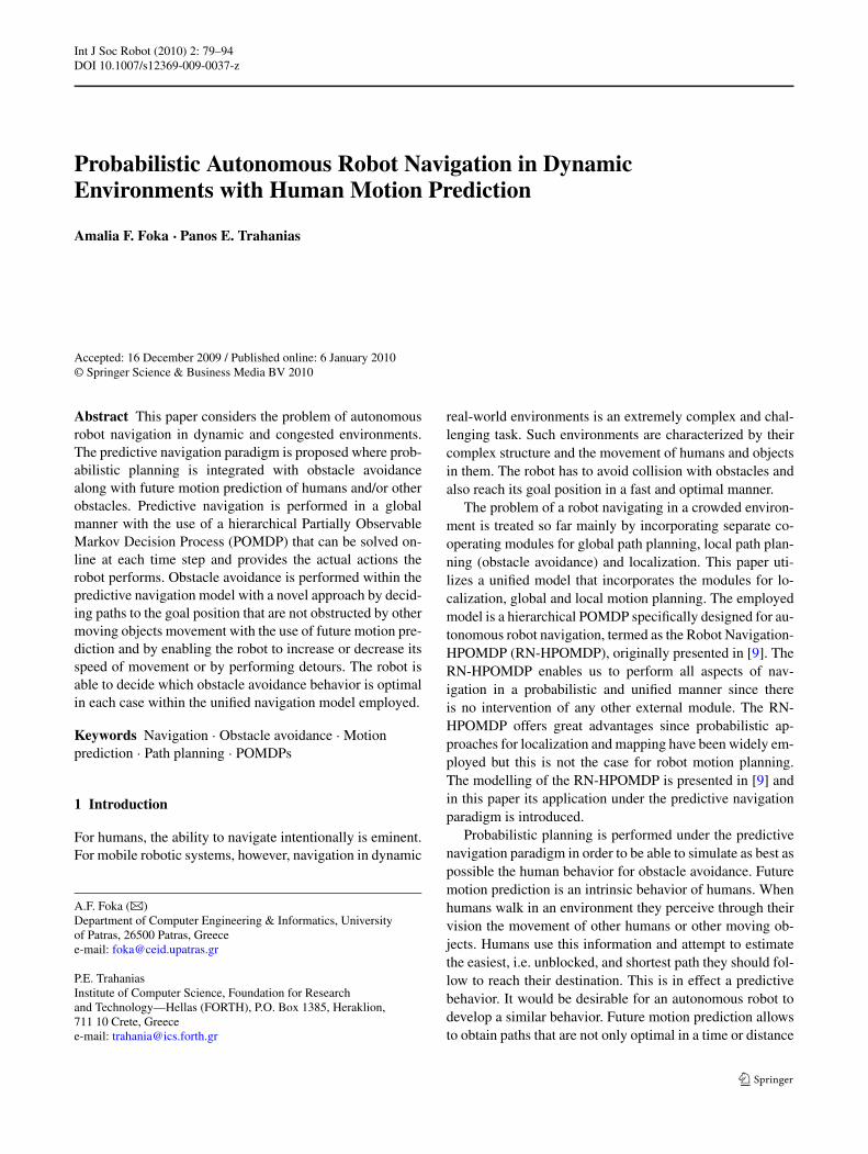
The HPs in an environment can be defined either man-ually or through an automated procedure. In Sect. 3.3, anautomated procedure for obtaining a map of HPs is pre-sented. The methodology for obtaining the long-term pre-diction is given for both cases where the HPs are definedmanually and when they are defined through a learned map.A primitive version of long term prediction with manuallydefined HPs was presented in Foka and Trahanias [7] eval-uated only in simple simulated environments. The manuallydefined hot points for the FORTH main entrance hall wherethe experiments were conducted are shown in Fig. 1. First,the methodology for obtaining the estimated destination po-sition of a moving object with manually defined HPs is pre-sented and then this approach is extended to be used with alearned map of HPs.

82 Int J Soc Robot (2010) 2: 79–94

Fig. 1 The “hot” points defined for the FORTH main entrance hall,marked with “x”

3.2 Estimation of a Moving Object’s Destination Position

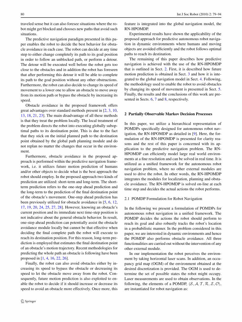
Once the points of interest of an environment are defined,then the long-term prediction refers to the prediction ofwhich Hot Point (HP) a moving obstacle is going to ap-proach. At each time step t , the tangent vector of the ob-stacle’s positions at times t − 1, t and the predicted positionat time t + 1 is taken. This tangent vector essentially deter-mines the global direction of the obstacle’s motion trajec-tory, termed as Global Direction of Obstacle (GDO). Thisdirection is employed to determine which HP a moving ob-stacle is going to approach. A HP is a candidate final des-tination point if it lies roughly in the direction of the eval-uated tangent vector, the GDO. In order to find such HPs,we establish a field-of-view, that is an angular area centeredat the GDO. HPs present in the field-of-view are possiblepoints to be reached, with a probability wi , according to aprobability model. The latter is defined as a Gaussian proba-bility distribution centered at the GDO with a standard devi-ation in proportion to the angular extent of the field-of-view.Thus, points of interest present in the center of the field-of-view are assigned a high probability, and points of interestpresent in the periphery of the field-of-view are assigned alower probability.

With this approach, at the beginning of the obstacle’smovement a multiple number of points of interest will bepresent in its field-of-view but as it continues its movementthe number of such points is decreased and finally it con-verges to a single point of interest.

In Fig. 2 an example of the procedure for long-term pre-diction with manually defined HPs is shown. At the begin-ning of the obstacle’s movement the long-term predictionobtained is shown in Fig. 2(a). It can be observed that at thispoint there are multiple candidate destination points for theobstacle’s movement. However, the destination point that in-fers that the moving objects is going to walk down the stairsis estimated as the most probable destination point of theobstacle’s movement as directed by the GDO. If the wholeobstacle motion trajectory, shown in the same figure, is ob-served it is obvious that the estimated destination point dic-tated by the long-term prediction methodology is not thecorrect one. However, the long-term prediction obtained isutilized partially. Therefore, when a long-term prediction

Fig. 2 An example of making long-term prediction for an object’smovement

is obtained, it is utilized partially only for a short intervalthat is close to the obstacle’s current position. Hence, thelong-term prediction when utilized only partially it provides

Int J Soc Robot (2010) 2: 79–94 83

a good estimate of the future motion of the obstacle’s move-ment. The partial utilization of the obtained long-term pre-diction is fully detailed in Sect. 4, where its integration to thenavigation model is explained. Additionally, the long-termprediction is updated at each time step, that is a short timeinterval, and hence bad estimates can be corrected quickly.Consequently, as the object has advanced through its motiontrajectory the long-term prediction estimate is closer to theactual destination point as shown in Fig. 2(b).

The example shown in Fig. 2 has been chosen such thatto demonstrate the weakness of using manually defined HPsand hence necessitate the use of the map of HPs. When theobstacle is close to the end of its motion trajectory, as shownin Fig. 2(c), there is no HP defined in the direction dictatedby the GDO. Instead, there are two HPs in the periphery ofthe GDO, and one of them is the actual destination point ofthe obstacle. However, the actual destination point will beassigned a low probability since it is located in the periph-ery of the GDO. The same holds for the other HP locatedwithin the field-of-view. In this scenario, if there was a mapof HPs available there would be defined a whole area of HPsinstead of two unique points. Specifically, in the area of themap under discussion there are two sofas where people of-ten go there and sit. When the map of HPs is constructedthe whole area covered by the sofas is determined as an in-teresting point instead of the two unique points in the cen-ter of the sofas that have been manually defined. Hence, wewould still have obtained a long-term prediction with highprobability. Additionally, the probability of each estimateddestination point is not determined only according to eachlocation within the field-of-view but also to the popularityof this point as determined through the learning procedure.

The map of HPs can also take care of the worst case sce-nario where there are not manually defined HPs present inthe field-of-view marginally and hence there would be noestimate available.

3.3 Map of Hot Points

An alternative approach to defining manually the hot pointsof the environment is to obtain a map of hot points of theenvironment through an automated procedure.

The map of hot points is a probabilistic map that givesfor each point of the environment the probability that thispoint is a hot point. This map is built off-line by a learningprocedure that uses motion traces of humans operating in theenvironment. At every step of each collected motion tracethe probabilities of the map of hot points are updated in asimilar manner to this used when building an occupancy gridmap of an environment from sensor readings.

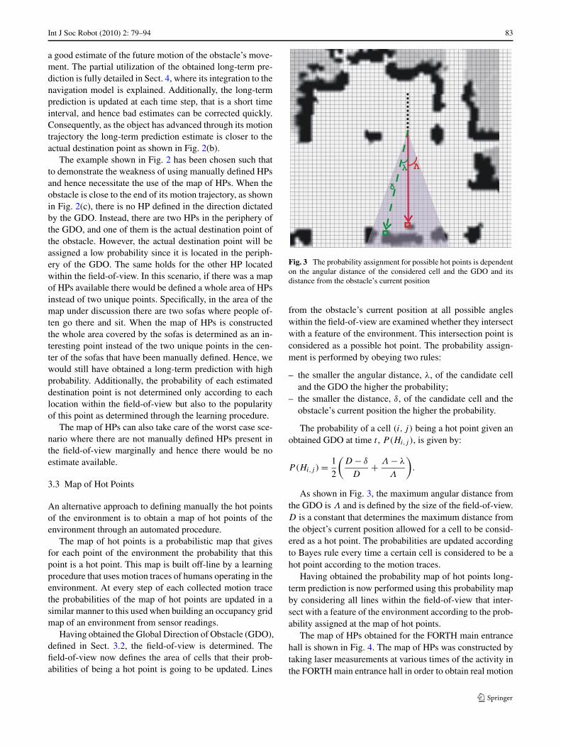
Having obtained the Global Direction of Obstacle (GDO),defined in Sect. 3.2, the field-of-view is determined. Thefield-of-view now defines the area of cells that their prob-abilities of being a hot point is going to be updated. Lines

Fig. 3 The probability assignment for possible hot points is dependenton the angular distance of the considered cell and the GDO and itsdistance from the obstacle’s current position

from the obstacle’s current position at all possible angleswithin the field-of-view are examined whether they intersectwith a feature of the environment. This intersection point isconsidered as a possible hot point. The probability assign-ment is performed by obeying two rules:

– the smaller the angular distance, λ, of the candidate celland the GDO the higher the probability;

– the smaller the distance, δ, of the candidate cell and theobstacle’s current position the higher the probability.

The probability of a cell (i, j) being a hot point given anobtained GDO at time t , P(Hi,j ), is given by:

P(Hi,j ) = 1

2

(D − δ

D+ Λ − λ

Λ

).

As shown in Fig. 3, the maximum angular distance fromthe GDO is Λ and is defined by the size of the field-of-view.D is a constant that determines the maximum distance fromthe object’s current position allowed for a cell to be consid-ered as a hot point. The probabilities are updated accordingto Bayes rule every time a certain cell is considered to be ahot point according to the motion traces.

Having obtained the probability map of hot points long-term prediction is now performed using this probability mapby considering all lines within the field-of-view that inter-sect with a feature of the environment according to the prob-ability assigned at the map of hot points.

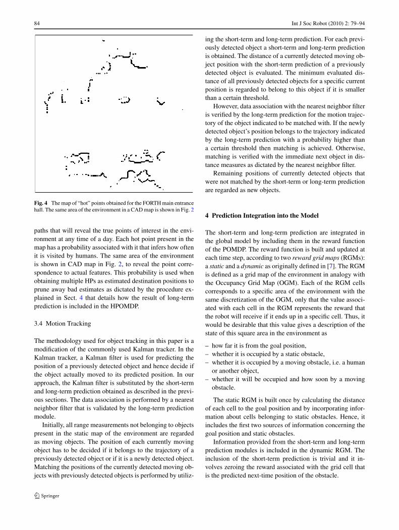
The map of HPs obtained for the FORTH main entrancehall is shown in Fig. 4. The map of HPs was constructed bytaking laser measurements at various times of the activity inthe FORTH main entrance hall in order to obtain real motion

84 Int J Soc Robot (2010) 2: 79–94

Fig. 4 The map of “hot” points obtained for the FORTH main entrancehall. The same area of the environment in a CAD map is shown in Fig. 2

paths that will reveal the true points of interest in the envi-ronment at any time of a day. Each hot point present in themap has a probability associated with it that infers how oftenit is visited by humans. The same area of the environmentis shown in CAD map in Fig. 2, to reveal the point corre-spondence to actual features. This probability is used whenobtaining multiple HPs as estimated destination positions toprune away bad estimates as dictated by the procedure ex-plained in Sect. 4 that details how the result of long-termprediction is included in the HPOMDP.

3.4 Motion Tracking

The methodology used for object tracking in this paper is amodification of the commonly used Kalman tracker. In theKalman tracker, a Kalman filter is used for predicting theposition of a previously detected object and hence decide ifthe object actually moved to its predicted position. In ourapproach, the Kalman filter is substituted by the short-termand long-term prediction obtained as described in the previ-ous sections. The data association is performed by a nearestneighbor filter that is validated by the long-term predictionmodule.

Initially, all range measurements not belonging to objectspresent in the static map of the environment are regardedas moving objects. The position of each currently movingobject has to be decided if it belongs to the trajectory of apreviously detected object or if it is a newly detected object.Matching the positions of the currently detected moving ob-jects with previously detected objects is performed by utiliz-

ing the short-term and long-term prediction. For each previ-ously detected object a short-term and long-term predictionis obtained. The distance of a currently detected moving ob-ject position with the short-term prediction of a previouslydetected object is evaluated. The minimum evaluated dis-tance of all previously detected objects for a specific currentposition is regarded to belong to this object if it is smallerthan a certain threshold.

However, data association with the nearest neighbor filteris verified by the long-term prediction for the motion trajec-tory of the object indicated to be matched with. If the newlydetected object’s position belongs to the trajectory indicatedby the long-term prediction with a probability higher thana certain threshold then matching is achieved. Otherwise,matching is verified with the immediate next object in dis-tance measures as dictated by the nearest neighbor filter.

Remaining positions of currently detected objects thatwere not matched by the short-term or long-term predictionare regarded as new objects.

4 Prediction Integration into the Model

The short-term and long-term prediction are integrated inthe global model by including them in the reward functionof the POMDP. The reward function is built and updated ateach time step, according to two reward grid maps (RGMs):a static and a dynamic as originally defined in [7]. The RGMis defined as a grid map of the environment in analogy withthe Occupancy Grid Map (OGM). Each of the RGM cellscorresponds to a specific area of the environment with thesame discretization of the OGM, only that the value associ-ated with each cell in the RGM represents the reward thatthe robot will receive if it ends up in a specific cell. Thus, itwould be desirable that this value gives a description of thestate of this square area in the environment as

– how far it is from the goal position,– whether it is occupied by a static obstacle,– whether it is occupied by a moving obstacle, i.e. a human

or another object,– whether it will be occupied and how soon by a moving

obstacle.

The static RGM is built once by calculating the distanceof each cell to the goal position and by incorporating infor-mation about cells belonging to static obstacles. Hence, itincludes the first two sources of information concerning thegoal position and static obstacles.

Information provided from the short-term and long-termprediction modules is included in the dynamic RGM. Theinclusion of the short-term prediction is trivial and it in-volves zeroing the reward associated with the grid cell thatis the predicted next-time position of the obstacle.

Int J Soc Robot (2010) 2: 79–94 85

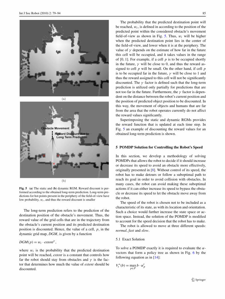
Fig. 5 (a) The static and (b) dynamic RGM. Reward discount is per-formed according to the obtained long-term prediction. Long-term pre-dictions for hot points present in the periphery of the field-of-view havelow probability, wi , and thus the reward discount is smaller

The long-term prediction refers to the prediction of thedestination position of the obstacle’s movement. Thus, thereward value of the grid cells that are in the trajectory fromthe obstacle’s current position and its predicted destinationposition is discounted. Hence, the value of a cell, p, in thedynamic grid map, DGM, is given by a function

DGM(p) = wi · extentγ ,

where wi is the probability that the predicted destinationpoint will be reached, extent is a constant that controls howfar the robot should stay from obstacles and γ is the fac-tor that determines how much the value of extent should bediscounted.

The probability that the predicted destination point willbe reached, wi , is defined in according to the position of thepredicted point within the considered obstacle’s movementfield-of-view as shown in Fig. 5. Thus, wi will be higherwhen the predicted destination point lies in the center ofthe field-of-view, and lower when it is at the periphery. Thevalue of γ depends on the estimate of how far in the futurethis cell will be occupied, and it takes values in the rangeof [0,1]. For example, if a cell p is to be occupied shortlyin the future, γ will be close to 0, and thus the reward as-signed to cell p will be small. On the other hand, if cell p

is to be occupied far in the future, γ will be close to 1 andthus the reward assigned to this cell will not be significantlydiscounted. The γ factor is defined such that the long-termprediction is utilized only partially for predictions that arenot too far in the future. Furthermore, the γ factor is depen-dent on the distance between the robot’s current position andthe position of predicted object position to be discounted. Inthis way, the movement of objects and humans that are farfrom the area that the robot operates currently do not affectthe reward values significantly.

Superimposing the static and dynamic RGMs providesthe reward function that is updated at each time step. InFig. 5 an example of discounting the reward values for anobtained long-term prediction is shown.

5 POMDP Solution for Controlling the Robot’s Speed

In this section, we develop a methodology of solvingPOMDPs that allows the robot to decide if it should increaseor decrease its speed to avoid an obstacle more effectively,originally presented in [8]. Without control of its speed, therobot has to make detours or follow a suboptimal path toreach its goal in order to avoid collision with obstacles. Inmany cases, the robot can avoid making these suboptimalactions if it can either increase its speed to bypass the obsta-cle or decrease its speed to let the obstacle move away fromthe robot.

The speed of the robot is chosen not to be included as acharacteristic of its state, as with its location and orientation.Such a choice would further increase the state space or ac-tion space. Instead, the solution of the POMDP is modifiedto account for the speed decision that the robot has to make.

The robot is allowed to move at three different speeds:normal, fast and slow.

5.1 Exact Solution

To solve a POMDP exactly it is required to evaluate the α-vectors that form a policy tree as shown in Fig. 6 by thefollowing equation as in [14]:

V ∗t (b) = max

p∈Pb · αt

p

86 Int J Soc Robot (2010) 2: 79–94

Fig. 6 An example policy tree of a POMDP with pairs of actions andspeeds

that searches all possible policy trees P , to maximize thisvalue function for the belief b. Recall that policy trees aredefined by having as nodes actions, a, that are connectedwith each possible observation, zi . To decide the action tobe executed as well the speed v of the robot, nodes are nowdefined by pairs of actions and speeds.

Since policy tree nodes are composed of action-speedpairs the value function of a policy tree has now to be eval-uated by considering the choice of the action as well as thespeed. The value function of a policy tree is evaluated by thefollowing equation, that has incorporated the speed decision:

Vpt (b)

=∑s∈S

b(s)

[Rm(s, a, v)

+ γ∑z∈Z

∑s′∈S

Om(z, s′, a, v)Tm(s, a, v, s′)V zp

t−1(s′)].

The above equation dictates that it is required to a have amodified version of the reward, transition and observationfunction. However, instead of defining new POMDP func-tions, the notion of the projected state is defined that allowsto use the original POMDP functions.

5.2 The Projected State

When the robot is in a state s and performs an action a witha velocity v, other than the normal velocity, it is expectedto end up with a certain probability in a state s′. Then, theprojected state is defined as the state sp , where if the robotexecutes the same action a, from state sp , with the normalvelocity it will end up with the same probability to state s′.Of course, if v is the normal velocity of the robot, then spis s.

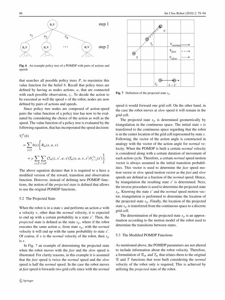
In Fig. 7 an example of determining the projected statewhen the robot moves with the fast and the slow speed isillustrated. For clarity reasons, in this example it is assumedthat the fast speed is twice the normal speed and the slowspeed is half the normal speed. In the case the robot movesat fast speed it forwards two grid cells since with the normal

Fig. 7 Definition of the projected state sp

speed it would forward one grid cell. On the other hand, inthe case the robot moves at slow speed it will remain in thegrid cell.

The projected state sp is determined geometrically bytriangulation in the continuous space. The initial state s istransferred to the continuous space regarding that the robotis in the center location of the grid cell represented by state s.Following, the vector of the action angle is constructed inanalogy with the vector of the action angle for normal ve-locity. When the POMDP is built a certain normal velocityis considered along with a certain duration of movement ofeach action cycle. Therefore, a certain normal speed motionvector is always assumed in the initial transition probabil-ities. This vector is used to determine the fast speed mo-tion vector or slow speed motion vector as the fast and slowspeeds are defined as a fraction of the normal speed. Hence,by triangulation the resulting state s′ is determined. Next,the inverse procedure is used to determine the projected statesp . Knowing the state s′ and the normal speed motion vec-tor, triangulation is performed to determine the location ofthe projected state sp . Finally, the location of the projectedstate sp is transferred from the continuous space to a discretegrid cell.

The determination of the projected state sp is an approx-imation according to the motion model of the robot used todetermine the transitions between states.

5.3 The Modified POMDP Functions

As mentioned above, the POMDP parameters are not alteredto include information about the robot velocity. Therefore,a formulation of Rm and Tm that relates them to the originalR and T functions that were built considering the normalvelocity of the robot only is required. This is achieved byutilizing the projected state of the robot.

Int J Soc Robot (2010) 2: 79–94 87

Having defined the projected state, the relation of Rm

and Tm to the original R and T , respectively, can now bedefined.

5.3.1 The Modified Transition Function Tm

By the definition of the projected state sp , the relation of Tm

to T is straightforward, and is written as:

Tm(s, a, v, s′) = T (sp, a, s′).

The above equation assumes that the transition probabili-ties for executing a certain rotation action a at normal speedare preserved when executing the same rotation action at thefast or slow speed. This is a safe approximation since in thecontext in which the change of speed is used, the robot willmove at a speed other than the normal speed for very shortintervals only, i.e. only when the robot has to bypass an ob-stacle with the fast speed or allow it move way by slowingdown. Furthermore, the fast and slow speed are defined asfractions of the normal speed that are rather small and there-fore the motion behavior of the robot does not change dra-matically.

5.3.2 The Modified Reward Function Rm

The definition of Rm is not as straightforward as for Tm.If Rm is simply defined as Rm(s, a, v) = R(sp, a), then therobot would always choose to move with the fast speed. Thisis because the fast speed will always get the robot closer tothe goal and thus the reward that it will receive will be big-ger. Instead, it is desirable that the robot moves at a differentspeed from its normal speed only if it has to avoid an obsta-cle. For that reason change of speed is penalized.

Rm(s, a, v) = R(sp, a) − penalty.

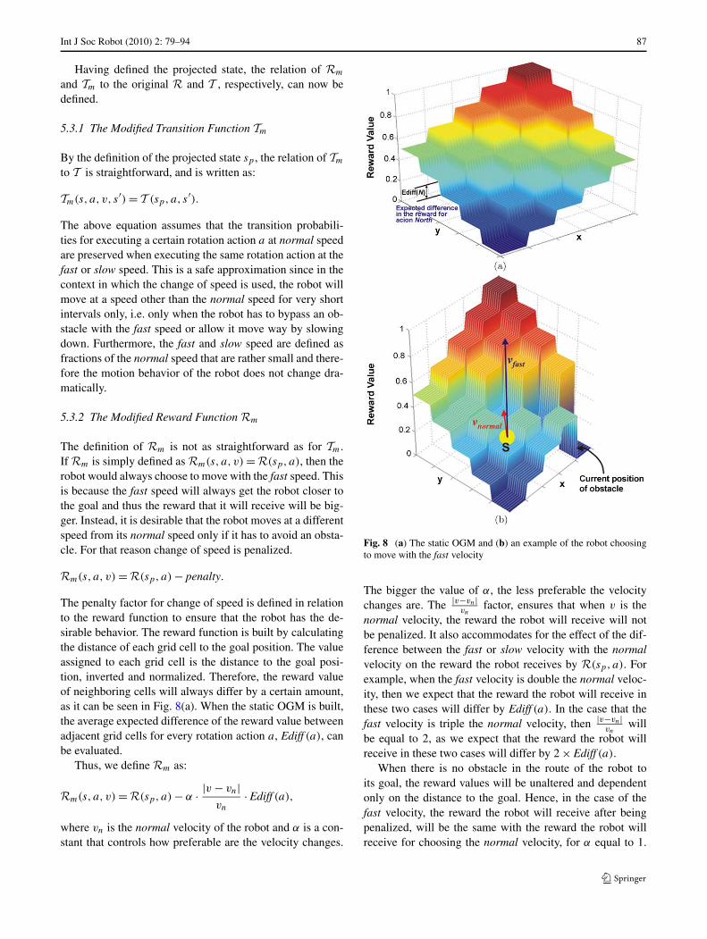
The penalty factor for change of speed is defined in relationto the reward function to ensure that the robot has the de-sirable behavior. The reward function is built by calculatingthe distance of each grid cell to the goal position. The valueassigned to each grid cell is the distance to the goal posi-tion, inverted and normalized. Therefore, the reward valueof neighboring cells will always differ by a certain amount,as it can be seen in Fig. 8(a). When the static OGM is built,the average expected difference of the reward value betweenadjacent grid cells for every rotation action a, Ediff (a), canbe evaluated.

Thus, we define Rm as:

Rm(s, a, v) = R(sp, a) − α · |v − vn|vn

· Ediff (a),

where vn is the normal velocity of the robot and α is a con-stant that controls how preferable are the velocity changes.

Fig. 8 (a) The static OGM and (b) an example of the robot choosingto move with the fast velocity

The bigger the value of α, the less preferable the velocitychanges are. The |v−vn|

vnfactor, ensures that when v is the

normal velocity, the reward the robot will receive will notbe penalized. It also accommodates for the effect of the dif-ference between the fast or slow velocity with the normalvelocity on the reward the robot receives by R(sp, a). Forexample, when the fast velocity is double the normal veloc-ity, then we expect that the reward the robot will receive inthese two cases will differ by Ediff (a). In the case that thefast velocity is triple the normal velocity, then |v−vn|

vnwill

be equal to 2, as we expect that the reward the robot willreceive in these two cases will differ by 2 × Ediff (a).

When there is no obstacle in the route of the robot toits goal, the reward values will be unaltered and dependentonly on the distance to the goal. Hence, in the case of thefast velocity, the reward the robot will receive after beingpenalized, will be the same with the reward the robot willreceive for choosing the normal velocity, for α equal to 1.

88 Int J Soc Robot (2010) 2: 79–94

In the case that there is an obstacle moving in the route ofthe robot to its goal, then the reward values of the cells thatare predicted to be occupied by the obstacle in the futurewill be discounted. Then, the reward the robot will receivefor fast velocity will be bigger than the reward for normalvelocity even after it is penalized for changing speed.

An example for this case is illustrated in Fig. 8(b). It isassumed that there is an obstacle moving in the environment.For clarity reasons, in this example the obstacle is assumedto occupy a single cell. The reward value of the cell that cor-responds to the obstacle’s current position is set to zero. Thereward value of the cells that are in the trajectory from theobstacle’s current position to its predicted destination posi-tion is discounted. The original reward value of these cellscan be seen in Fig. 8(a). The discount of the reward valuesis not the same for all cells, since it depends on the esti-mate of how far in the future each cell will be occupied.The robot is currently at the cell denoted with s. If the robotmoves with the normal velocity, it will maximize its rewardwhen executing one of the suboptimal actions to reach thegoal since the reward for executing action North-East hasbeen discounted due to the long-term prediction. When thereward values for the fast velocity are evaluated, it can beseen that the reward for executing action North-East will bethe maximum. That is because the robot will end up in astate where its reward has not been discounted due to long-term prediction and even when the expected difference in thereward values for action North-East is deducted it will stillremain bigger than all other rewards. Hence, the robot willmove with the fast velocity and bypass the moving obstacle.

In the case of the slow speed, the reward the robot will re-ceive for executing any action from the projected state willalways be smaller than the reward the robot will receivefor choosing the normal speed, when there is no obstacle.This reward will be further decreased by the penalty factor.Therefore, for the robot to choose the slow speed, the rewardit receives for the normal and fast speed has to be smaller.This will be the case when there is an obstacle very close tothe robot and did not have a long-term prediction to be ableto avoid it by increasing its speed.

5.3.3 The Modified Observation Function Om

The relation of Om to the original observation function O,using the projected state sp , is straightforward and is writtenas:

Om(s, a, v, z) = O(sp, a, z).

The above definition holds due to the way the observationset has been defined in Sect. 2.1. An observation is actuallythe distance the robot travelled when it has executed a cer-tain action a. As a result, the relation of Om to the originalobservation function O is in analogy with the relation to thedefinition for the transition function.

5.4 Approximation Methods

The described methodology for controlling the robot’s speedcan also be applied with any of the approximation methodsreviewed in [11] with the use of the modified POMDP func-tions.

In the case that the MLS heuristic is used the optimalvalue function is computed as:

V ∗t (s) = max

a∈A,v∈VQm

(arg max

s∈S(b(s)), a, v

)

where the modified Q-function, Qm, is now defined as:

Qtm(s, a, v) = Rm(s, a, v) + γ

∑s′∈S

Tm(s, a, v, s′)Vt−1(s′).

In the case that the voting heuristic is used the optimalvalue function is given by:

V ∗t (s) = max

a∈A,v∈V

∑s∈S

b(s)δ(πMDP(s), a, v)

where

πMDP(s) = arg maxa∈A,v∈V

Qm(s, a, v)

and

δ(ai, vi, aj , vj ) ={

1, if ai = aj and vi = vj ,

0, if ai �= aj or vi �= vj .

In the same manner the modified POMDP functions canbe applied to other approximation methods present in theliterature.

6 Results

This section presents experimental results that validate theproposed approach for autonomous robot navigation. Ini-tially the experimental configuration for the real-world en-vironment as well as the simulated one is presented. Finally,results that demonstrate the behavior in general of the pre-dictive navigation framework are illustrated.

6.1 Experimental Configurations

For testing the performance of the proposed framework, wehave performed extensive tests with both real and simulateddata. All real data have been assessed on Lefkos, an iRo-bot B21r robotic platform of our lab, while acting in variousindoor areas of FORTH.

Int J Soc Robot (2010) 2: 79–94 89

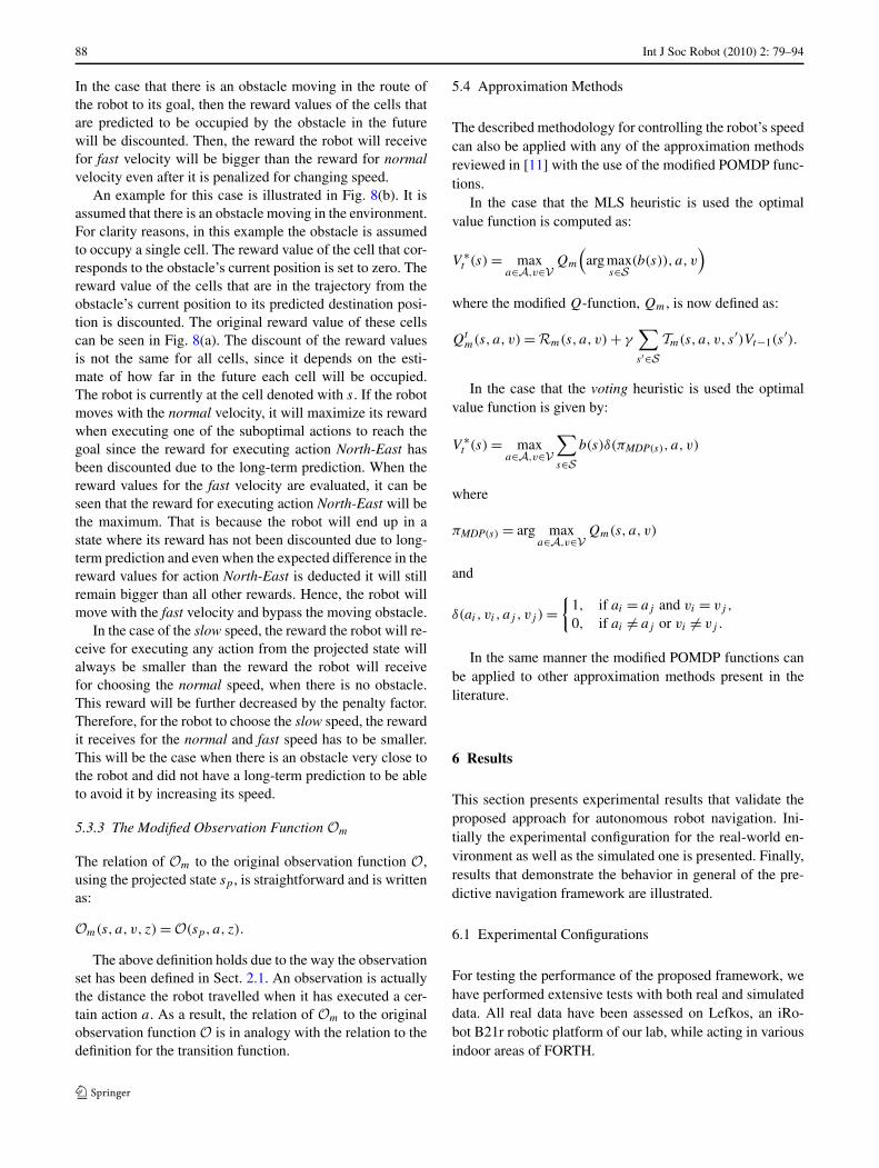
Fig. 9 Avoiding two moving objects with a detour. The robot detects early in its movement that its path to the goal point, the stairs, will becompletely blocked by the two persons moving. Hence, it starts making a detour well before it faces any of the two persons

6.2 Real Environment Experiments

In this section a representative set of result of the robot op-erating in the FORTH main entrance hall is shown. The ro-bot was set to operate for more than 70 hours. The envi-ronment was modelled with a RN-HPOMDP with size ofthe set states, actions and observations being respectively|S| = 18,411,520, |A| = 256 and |Z| = 24. This resultsto grid cells of actual size 10 cm2. Experiments were per-formed in a dynamic environment where people were mov-ing within it. In all cases the proposed navigation model hasshown a robust behavior in reaching the assigned goal pointsand avoiding humans or other objects. Following, samplepaths the robot followed to reach its goal position by demon-strating the four main behaviors it uses to avoid obstacle arepresented.

6.2.1 Avoiding Obstacles with a Detour

In this experiment we demonstrate how the robot avoids twohumans moving in the environment in such a manner thatthey block its route to the goal position. If there were nohumans or other objects moving, the robot would followa straight path to its goal, defined for our experiments asshown in Fig. 9. In our experiment two humans are mov-ing in the environment. One of them is moving towards thestraight path that the robot would follow to reach its goaland the other one is moving in a straight direction vertical tothe one the robot would follow. As shown in the figures therobot detects the moving humans and obtains the long-termprediction of their movement and hence decides to make a

detour by turning. The decision the robot makes about thedetour is long before the robot actually faces the moving hu-mans and where a local obstacle avoidance method woulddecide to make a detour.

6.2.2 Avoiding Obstacles by Following a Replanned Path

In this experiment we show that the robot can decide to fol-low a completely different path from the one it would followin a static environment in order to avoid humans moving. Itis obvious from the images shown in Fig. 10, that the optimalpath to reach the goal position if the robot was operating in astatic environment it would be to follow a straight trajectory.In our experiment, a human was moving to block this staticoptimal path and the robot decided to follow a completelydifferent path, i.e. follow a trajectory that goes behind thebuilding’s column to reach the goal position.

6.2.3 Avoiding Obstacles by Increasing the Robot’s Speed

In the experiment shown in Fig. 11 the robot increases itsspeed to bypass the human’s movement in order to reachits goal position without the need of making a detour. Thehuman’s movement is perceived by the robot from the be-ginning and hence it obtains the long-term prediction earlyenough to decide to increase its speed to bypass the human’spredicted motion trajectory. When the robot has passed thehuman’s motion trajectory its decreases its speed to normalto continue its movement.

90 Int J Soc Robot (2010) 2: 79–94

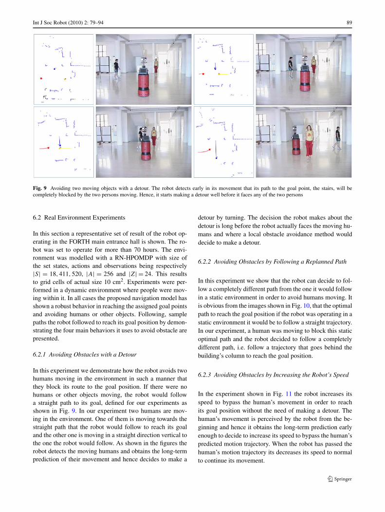
Fig. 10 Deciding to follow a completely different path. The robot hasto follow a simple straight path to reach its goal position that is thestarting point of movement of the person present in the environment.

However, the robot detects early enough that the person moves towardsits and decides to change its path to the goal by going around the build-ing’s column

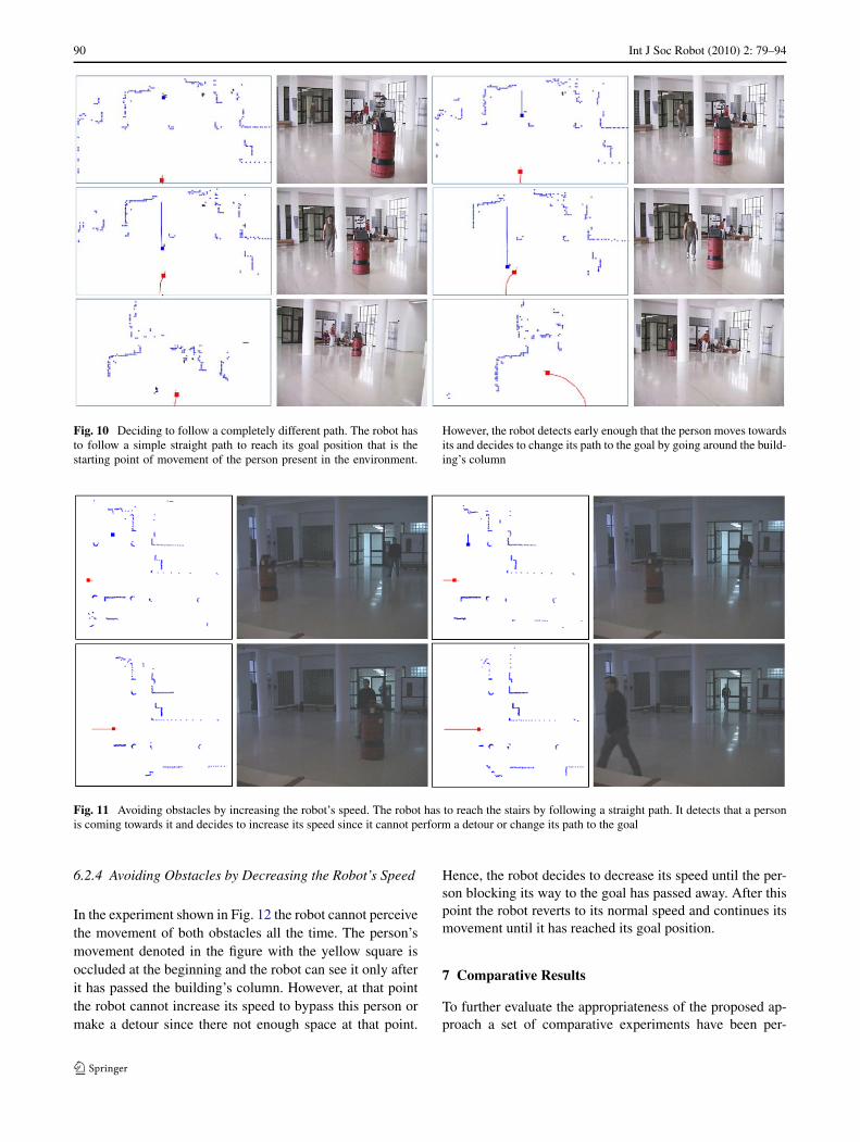
Fig. 11 Avoiding obstacles by increasing the robot’s speed. The robot has to reach the stairs by following a straight path. It detects that a personis coming towards it and decides to increase its speed since it cannot perform a detour or change its path to the goal

6.2.4 Avoiding Obstacles by Decreasing the Robot’s Speed

In the experiment shown in Fig. 12 the robot cannot perceivethe movement of both obstacles all the time. The person’smovement denoted in the figure with the yellow square isoccluded at the beginning and the robot can see it only afterit has passed the building’s column. However, at that pointthe robot cannot increase its speed to bypass this person ormake a detour since there not enough space at that point.

Hence, the robot decides to decrease its speed until the per-son blocking its way to the goal has passed away. After thispoint the robot reverts to its normal speed and continues itsmovement until it has reached its goal position.

7 Comparative Results

To further evaluate the appropriateness of the proposed ap-proach a set of comparative experiments have been per-

Int J Soc Robot (2010) 2: 79–94 91

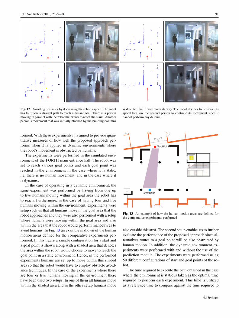
Fig. 12 Avoiding obstacles by decreasing the robot’s speed. The robothas to follow a straight path to reach a distant goal. There is a personmoving in parallel with the robot that wants to reach the stairs. Anotherperson’s movement that was initially blocked by the building columns

is detected that it will block its way. The robot decides to decrease itsspeed to allow the second person to continue its movement since itcannot perform any detours

formed. With these experiments it is aimed to provide quan-titative measures of how well the proposed approach per-forms when it is applied in dynamic environments wherethe robot’s movement is obstructed by humans.

The experiments were performed in the simulated envi-ronment of the FORTH main entrance hall. The robot wasset to reach various goal points and each goal point wasreached in the environment in the case where it is static,i.e. there is no human movement, and in the case where itis dynamic.

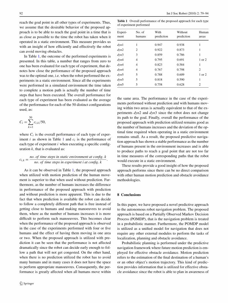
In the case of operating in a dynamic environment, thesame experiment was performed by having from one upto five humans moving within the goal area the robot hasto reach. Furthermore, in the case of having four and fivehumans moving within the environment, experiments weresetup such us that all humans move in the goal area that therobot approaches and they were also performed with a setupwhere humans were moving within the goal area and alsowithin the area that the robot would perform manoeuvres toavoid humans. In Fig. 13 an example is shown of the humanmotion areas defined for the comparative experiments per-formed. In this figure a sample configuration for a start anda goal point is shown along with a shaded area that denotesthe area within the robot would choose to move to reach thegoal point in a static environment. Hence, in the performedexperiments humans are set up to move within this shadedarea so that the robot would have to employ obstacle avoid-ance techniques. In the case of the experiments where thereare four or five humans moving in the environment therehave been used two setups. In one of them all humans movewithin the shaded area and in the other setup humans move

Fig. 13 An example of how the human motion areas are defined forthe comparative experiments performed

also outside this area. The second setup enables us to furtherevaluate the performance of the proposed approach since al-ternatives routes to a goal point will be also obstructed byhuman motion. In addition, the dynamic environment ex-periments were performed with and without the use of theprediction module. The experiments were performed using50 different configurations of start and goal points of the ro-bot.

The time required to execute the path obtained in the casewhere the environment is static is taken as the optimal timerequired to perform each experiment. This time is utilizedas a reference time to compare against the time required to

92 Int J Soc Robot (2010) 2: 79–94

reach the goal point in all other types of experiments. Thus,we assume that the desirable behavior of the proposed ap-proach is to be able to reach the goal point in a time that isas close as possible to the time the robot has taken when itoperated in a static environment. This measure provides uswith an insight of how efficiently and effectively the robotcan avoid moving obstacles.

In Table 1, the outcome of the performed experiments ispresented. In this table, a number that ranges from zero toone has been evaluated for each type of experiment, that de-notes how close the performance of the proposed approachwas to the optimal one, i.e. when the robot performed the ex-periments in a static environment. Since all the experimentswere performed in a simulated environment the time takento complete a motion path is actually the number of timesteps that have been executed. The overall performance foreach type of experiment has been evaluated as the averageof the performance for each of the 50 distinct configurationsused, as:

Ci =50∑

k=1

ci,k/50,

where Ci is the overall performance of each type of exper-iment i as shown in Table 1 and ci is the performance ofeach type of experiment i when executing a specific config-uration k, that is evaluated as:

ci,k = no. of time steps in static environment at config. k

no. of time steps in experiment i at config. k.

As it can be observed in Table 1, the proposed approachwhen utilized with motion prediction of the human move-ment is superior to that when used without prediction. Fur-thermore, as the number of humans increases the differencein performance of the proposed approach with predictionand without prediction is more apparent. This is due to thefact that when prediction is available the robot can decideto follow a completely different path that is free instead ofgetting close to humans and making manoeuvres to avoidthem, where as the number of humans increases it is moredifficult to perform such manoeuvres. This becomes clearwhen the performance of the proposed approach is observedin the case of the experiments performed with four or fivehumans and the effect of having them moving in one areaor two. When the proposed approach is utilized with pre-diction it can be seen that the performance is not affecteddramatically since the robot can decide early enough to fol-low a path that will not get congested. On the other hand,when there is no prediction utilized the robot has to avoidmany humans and in many cases it does not have the spaceto perform appropriate manoeuvres. Consequently, the per-formance is greatly affected when all humans move within

Table 1 Overall performance of the proposed approach for each typeof experiment performed

Experi- No. of With Without Humanment humans prediction prediction areas

dyn1 1 0.947 0.938 1

dyn2 2 0.922 0.873 1

dyn3 3 0.859 0.786 1

dyn4 4 0.795 0.691 1 or 2

dyn4 4 0.823 0.584 1

dyn4 4 0.767 0.798 2

dyn5 5 0.788 0.609 1 or 2

dyn5 5 0.818 0.590 1

dyn5 5 0.758 0.628 2

the same area. The performance in the case of the experi-ments performed without prediction and with humans mov-ing within two areas is actually equivalent to that of the ex-periments dyn2 and dyn3 since the robot does not changeits path to the goal. Finally, overall the performance of theproposed approach with prediction utilized remains good asthe number of humans increases and the deviation of the op-timal time required when operating in a static environmentremains small. As a result, the proposed predictive naviga-tion approach has shown a stable performance as the numberof humans present in the environment increases and is ableto produce paths to reach a goal point that are not too farin time measures of the corresponding paths that the robotwould execute in a static environment.

These results provide a good insight of how the proposedapproach performs since there can be no direct comparisonwith other human motion prediction and obstacle avoidancemethodologies.

8 Conclusions

In this paper, we have proposed a novel predictive approachto the autonomous robot navigation problem. The proposedapproach is based on a Partially Observed Markov DecisionProcess (POMDP), that is the navigation problem is treatedin a probabilistic manner. Furthermore, the POMDP modelis utilized as a unified model for navigation that does notrequire any other external modules to perform the tasks oflocalization, planning and obstacle avoidance.

Probabilistic planning is performed under the predictivenavigation framework where future motion prediction is em-ployed for effective obstacle avoidance. Motion predictionrefers to the estimation of the final destination of a human’sor an other object’s motion trajectory. This kind of predic-tion provides information that is utilized for effective obsta-cle avoidance since the robot is able to plan in awareness of

Int J Soc Robot (2010) 2: 79–94 93

predicted changes in the environment. The predictive nav-igation framework provides the robot the option to choosethe suitable behavior among the following four for obstacleavoidance:

– execute a detour– change completely the planned path to the goal position– increase its speed to bypass the obstacles– decrease its speed to let the obstacles move away.

The proposed approach is capable of performing obsta-cle avoidance in a unique manner as compared to standardmethods that perform manoeuvres to avoid obstacles locallyonly when the robot gets close to them. The performance ofthe predictive navigation approach has been experimentallyvalidated and the results have shown that it can provide opti-mal paths that are affected the least possible by other movingobstacle’s movement.

References

1. Bennewitz M, Burgard W, Cielniak G, Thrun S (2005) Learningmotion patterns of people for compliant robot motion. Int J RobotRes 24(1)

2. Borenstein J, Koren Y (1991) The Vector Field Histogram—fastobstacle avoidance for mobile robots. IEEE Trans Robot Autom7(3):278–288

3. Brock O, Khatib O (1999) High-speed navigation using the globaldynamic window approach. In: Proceedings of the IEEE interna-tional conference on robotics & automation (ICRA)

4. Bruce A, Gordon G (2004) Better motion prediction for people-tracking. In: Proceedings of the IEEE international conference onrobotics & automation (ICRA)

5. Chang CC, Song KT (1996) Dynamic motion planning based onreal-time obstacle prediction. In: Proceedings of the IEEE in-ternational conference on robotics & automation (ICRA), vol 3,pp 2402–2407

6. Elganar A, Gupta K (1998) Motion prediction of moving objectsbased on autoregressive model. IEEE Trans Syst Man CybernPart A 28(6):803–810

7. Foka A, Trahanias P (2002) Predictive autonomous robot naviga-tion. In: Proceedings of the IEEE/RSJ international conference onintelligent robots & systems (IROS)

8. Foka A, Trahanias P (2003) Predictive control of robot velocityto avoid obstacles in dynamic environments. In: Proceedings ofthe IEEE/RSJ international conference on intelligent robots & sys-tems (IROS)

9. Foka AF, Trahanias PE (2007) Real-time hierarchical POMDPSfor autonomous robot navigation. Robot Auton Syst 55(7):561–571

10. Fox D, Burgard W, Thrun S (1997) The dynamic window ap-proach to collision avoidance. IEEE Robot Autom Mag 4(1):23–33

11. Hauskrecht M (2000) Value function approximations for PartiallyObservable Markov Decision Processes. J Artif Intell Res 13:33–95

12. Kehtarnavaz N, Li S (1988) A collision-free navigation schemein the presence of moving obstacles. In: CVPR’88 (IEEE com-puter society conference on computer vision and pattern recog-nition, Ann Arbor, MI, 5–9 June 1988). Computer Society Press,Washington, pp 808–813

13. Khatib O (1986) Real-time obstacle avoidance for robot manipu-lator and mobile robots. Int J Robot Res 5(1):90–98

14. Littman ML, Goldsmith J, Mundhenk M (1998) The computa-tional complexity of probabilistic planning. J Artif Intell Res 9:1–36

15. Lu F, Milios E (1998) Robot pose estimation in unknown environ-ments by matching 2d range scans. J Intell Robot Syst 18:249–275

16. Müller J, Stachniss C, Arras K, Burgard W (2009) Sociallyinspired motion planning for mobile robots in populated en-vironments. In: International Conference on Cognitive Systems(CogSys), Karlsruhe, Germany, 2008

17. Nam YS, Lee BH, Kim MS (1996) View-time based moving ob-stacle avoidance using stochastic prediction of obstacle motion.In: Proceedings of the 1996 IEEE international conference on ro-botics and automation, pp 1081–1086

18. Ogren P, Leonard N (2005) A convergent dynamic window ap-proach to obstacle avoidance. IEEE Trans Robot 21(2):188–195

19. Oliver S, Saptharishi M, Dolan J, Trebi-Ollennu A, Khosla P(2000) Multi-robot path planning by predicting structure in a dy-namic environment. In: Proceedings of the first IFAC conferenceon mechatronic systems, vol II, pp 593–598

20. Ortega JG, Camacho EF (1996) Mobile robot navigation in a par-tially structured static environment, using neural predictive con-trol. Control Eng Pract 4(12):1669–1679

21. Petti S, Fraichard T (2005) Safe motion planning in dynamic envi-ronments. In: Proceedings of the IEEE/RSJ international confer-ence on intelligent robots & systems (IROS), pp 2210– 2215

22. Rohrmuller F, Althoff M, Wollherr D, Buss M (2008) Probabilisticmapping of dynamic obstacles using Markov chains for replanningin dynamic environments. In: IROS, pp 2504–2510

23. Stachniss C, Burgard W (2002) An integrated approach to goal-directed obstacle avoidance under dynamic constraints for dy-namic environments. In: Proceedings of the IEEE/RSJ interna-tional conference on intelligent robots & systems (IROS)

24. Tadokoro S, Ishikawa Y, Takebe T, Takamori T (1993) Stochasticprediction of human motion and control of robots in the service ofhuman. In: Proceedings of the 1993 IEEE international conferenceon systems, man and cybernetics, vol 1, pp 503–508

25. Tadokoro S, Hayashi M, Manabe Y (1995) On motion planning ofmobile robots which coexist and cooperate with human. In: Pro-ceedings of the 1995 IEEE/RSJ international conference on intel-ligent robots and systems, pp 518–523

26. Vasquez D, Fraichard T (2004) Motion prediction for moving ob-jects: a statistical approach. In: Proceedings of the IEEE interna-tional conference on robotics & automation (ICRA)

27. Yung NHC, Ye C (1998) Avoidance of moving obstacles throughbehavior fusion and motion prediction. In: IEEE international con-ference on systems, man and cybernetics, pp 3424–3429

28. Zhu Q (1991) Hidden Markov Model for dynamic obstacle avoid-ance of mobile robot navigation. IEEE Trans Robot Autom7(3):390–397

Amalia F. Foka was born in Patras, Greece in 1976. She received theB.Eng. degree in Computer Systems Engineering and the M.Sc. degreein Advanced Control from UMIST, UK in 1998 and 1999 respectively.She received the Ph.D. degree in 2005 from the Department of Com-puter Science, University of Crete, Greece. She currently is a visitinglecturer at the Department of Computer Engineering and Informatics,University of Patras, Greece. Her research interests include roboticsand artificial intelligence.

Panos E. Trahanias received his Ph.D. in Computer Science from theNational Technical University of Athens, Greece. Currently he is a Pro-fessor with the University of Crete, Greece and the Foundation for Re-search and Technology—Hellas (FORTH). From 1991 to 1993 he was

94 Int J Soc Robot (2010) 2: 79–94

with the Department of Electrical and Computer Engineering, Univer-sity of Toronto, Canada, as a Research Associate. He has participated inmany RTD programs in image analysis at the University of Toronto andhas been a consultant to SPAR Aerospace Ltd., Toronto. Since 1993 heis with the University of Crete and FORTH; currently, he is the Directorof Graduate Studies, Department of Computer Science, University ofCrete, and the Head of the Computational Vision and Robotics Labo-ratory at FORTH, where he is engaged in research and RTD projects inautonomous mobile platforms, sensory technologies, computational vi-

sion, mixed realities and human-robot interaction. Professor Trahaniashas extensive experience in the execution and co-ordination of largeresearch projects. Moreover, his work has been published extensivelyin scientific journals and conferences. He has participated in the Pro-gramme Committees of numerous International Conferences; he hasbeen the General Chair of Computer Graphics International 2004, andwill be General Co-Chair of Eurographics 2008 and the European Con-ference on Computer Vision 2010.