Probabilistic Logics and Probabilistic Networks

Probabilistic Logics and Probabilistic Networks

Rolf Haenni∗†

Jan-Willem Romeijn‡

Gregory Wheeler§

Jon Williamson¶

Abstract

While in principle probabilistic logics might be applied to solve a rangeof problems, in practice they are rarely applied at present. This is per-haps because they seem disparate, complicated, and computationally in-tractable. However, we shall argue in this programmatic paper that sev-eral approaches to probabilistic logic fit into a simple unifying framework:logically complex evidence can be used to associate probability intervalsor probabilities with sentences.

Specifically, we show in Part I that there is a natural way to presenta question posed in probabilistic logic, and that various inferential pro-cedures provide semantics for that question: the standard probabilisticsemantics (which takes probability functions as models), probabilistic ar-gumentation (which considers the probability of a hypothesis being a log-ical consequence of the available evidence), evidential probability (whichhandles reference classes and frequency data), classical statistical inference(in particular the fiducial argument), Bayesian statistical inference (whichascribes probabilities to statistical hypotheses), and objective Bayesianepistemology (which determines appropriate degrees of belief on the basisof available evidence).

Further, we argue, there is the potential to develop computationallyfeasible methods to mesh with this framework. In particular, we show inPart II how credal and Bayesian networks can naturally be applied as acalculus for probabilistic logic. The probabilistic network itself dependsupon the chosen semantics, but once the network is constructed, commonmachinery can be applied to generate answers to the fundamental questionintroduced in Part I.

∗Dept. of Engineering and Information Technologies, Bern University of Applied Science†Institute of Computer Science and Applied Mathematics, University of Bern‡Department of Philosophy, University of Groningen§Department of Computer Science & Centre for Research in Artificial Intelligence, New

University of Lisbon¶Department of Philosophy & Centre for Reasoning, University of Kent

1

Contents

I Probabilistic Logics 5

1 Introduction 51.1 The Potential of Probabilistic Logic . . . . . . . . . . . . . . . . 61.2 Overview of the Paper . . . . . . . . . . . . . . . . . . . . . . . . 61.3 Philosophical and Historical Background . . . . . . . . . . . . . . 81.4 Notation and Formal Setting . . . . . . . . . . . . . . . . . . . . 9

2 Standard Probabilistic Semantics 102.1 Background . . . . . . . . . . . . . . . . . . . . . . . . . . . . . . 11

2.1.1 Kolmogorov Probabilities . . . . . . . . . . . . . . . . . . 112.1.2 Interval-Valued Probabilities . . . . . . . . . . . . . . . . 122.1.3 Imprecise Probabilities . . . . . . . . . . . . . . . . . . . . 142.1.4 Convexity . . . . . . . . . . . . . . . . . . . . . . . . . . . 15

2.2 Representation . . . . . . . . . . . . . . . . . . . . . . . . . . . . 152.3 Interpretation . . . . . . . . . . . . . . . . . . . . . . . . . . . . . 17

3 Probabilistic Argumentation 183.1 Background . . . . . . . . . . . . . . . . . . . . . . . . . . . . . . 183.2 Representation . . . . . . . . . . . . . . . . . . . . . . . . . . . . 213.3 Interpretation . . . . . . . . . . . . . . . . . . . . . . . . . . . . . 22

3.3.1 Generalizing the Standard Semantics . . . . . . . . . . . . 223.3.2 Premises from Unreliable Sources . . . . . . . . . . . . . . 24

4 Evidential Probability 274.1 Background . . . . . . . . . . . . . . . . . . . . . . . . . . . . . . 27

4.1.1 Calculating Evidential Probability . . . . . . . . . . . . . 284.1.2 Evidential Probability and Partial Entailment . . . . . . . 30


4.3.1 First-order Evidential Probability . . . . . . . . . . . . . . 324.3.2 Counter-Factual Evidential Probability . . . . . . . . . . 334.3.3 Second-Order Evidential Probability . . . . . . . . . . . . 34

5 Statistical Inference 355.1 Background . . . . . . . . . . . . . . . . . . . . . . . . . . . . . . 35

5.1.1 Classical Statistics as Inference? . . . . . . . . . . . . . . 355.1.2 Fiducial Probability . . . . . . . . . . . . . . . . . . . . . 375.1.3 Evidential Probability and Direct Inference . . . . . . . . 40

5.2 Representation . . . . . . . . . . . . . . . . . . . . . . . . . . . . 415.2.1 Fiducial Probability . . . . . . . . . . . . . . . . . . . . . 425.2.2 Evidential Probability and the Fiducial Argument . . . . 42

5.3 Interpretation . . . . . . . . . . . . . . . . . . . . . . . . . . . . . 435.3.1 Fiducial Probability . . . . . . . . . . . . . . . . . . . . . 435.3.2 Evidential Probability . . . . . . . . . . . . . . . . . . . . 44

2

6 Bayesian Statistical Inference 456.1 Background . . . . . . . . . . . . . . . . . . . . . . . . . . . . . . 456.2 Representation . . . . . . . . . . . . . . . . . . . . . . . . . . . . 46

6.2.1 Infinitely Many Hypotheses . . . . . . . . . . . . . . . . . 476.2.2 Interval-Valued Priors and Posteriors . . . . . . . . . . . . 49

6.3 Interpretation . . . . . . . . . . . . . . . . . . . . . . . . . . . . . 496.3.1 Interpretation of Probabilities . . . . . . . . . . . . . . . . 496.3.2 Bayesian confidence intervals . . . . . . . . . . . . . . . . 50

7 Objective Bayesianism 517.1 Background . . . . . . . . . . . . . . . . . . . . . . . . . . . . . . 51

7.1.1 Determining Objective Bayesian Degrees of Belief . . . . 517.1.2 Constraints on Degrees of Belief . . . . . . . . . . . . . . 527.1.3 Propositional Languages . . . . . . . . . . . . . . . . . . . 537.1.4 Predicate Languages . . . . . . . . . . . . . . . . . . . . . 547.1.5 Objective Bayesianism in Perspective . . . . . . . . . . . 55


II Probabilistic Networks 58

8 Credal and Bayesian Networks 588.1 Kinds of Probabilistic Network . . . . . . . . . . . . . . . . . . . 59

8.1.1 Extensions . . . . . . . . . . . . . . . . . . . . . . . . . . 608.1.2 Extensions and Coordinates . . . . . . . . . . . . . . . . . 618.1.3 Parameterised Credal Networks . . . . . . . . . . . . . . . 63

8.2 Algorithms for Probabilistic Networks . . . . . . . . . . . . . . . 638.2.1 Requirements of the Probabilistic Logic Framework . . . . 648.2.2 Compiling Probabilistic Networks . . . . . . . . . . . . . . 658.2.3 The Hill-Climbing Algorithm for Credal Networks . . . . 668.2.4 Complex Queries and Parameterised Credal Networks . . 68

9 Networks for the Standard Semantics 699.1 The Poverty of Standard Semantics . . . . . . . . . . . . . . . . . 699.2 Constructing a Credal Net . . . . . . . . . . . . . . . . . . . . . . 709.3 Dilation and Independence . . . . . . . . . . . . . . . . . . . . . 74

10 Networks for Probabilistic Argumentation 7510.1 Probabilistic Argumentation with Credal Sets . . . . . . . . . . . 7510.2 Constructing and Applying the Credal Network . . . . . . . . . . 76

11 Networks for Evidential Probability 7711.1 First-Order Evidential Probability . . . . . . . . . . . . . . . . . 7811.2 Second-Order Evidential Probability . . . . . . . . . . . . . . . . 79

12 Networks for Statistical Inference 8012.1 Functional Models and Networks . . . . . . . . . . . . . . . . . . 81

12.1.1 Capturing the Fiducial Argument in a Network . . . . . . 8112.1.2 Aiding Fiducial Inference with Networks . . . . . . . . . . 8112.1.3 Trouble with step-by-step fiducial probability . . . . . . . 83

3

12.2 Evidential Probability and the Fiducial Argument . . . . . . . . 8412.2.1 First-order EP and the Fiducial Argument . . . . . . . . 8412.2.2 Second-order EP and the Fiducial Argument . . . . . . . 84

13 Networks for Bayesian Statistical Inference 8513.1 Credal Networks as Statistical Hypotheses . . . . . . . . . . . . . 85

13.1.1 Construction of the Credal Network . . . . . . . . . . . . 8513.1.2 Computational Advantages of Using the Credal Network . 87

13.2 Extending Statistical Inference with Credal Networks . . . . . . . 8813.2.1 Interval-Valued Likelihoods . . . . . . . . . . . . . . . . . 8813.2.2 Logically Complex Statements with Statistical Hypotheses 90

14 Networks for Objective Bayesianism 9014.1 Propositional Languages . . . . . . . . . . . . . . . . . . . . . . . 9114.2 Predicate Languages . . . . . . . . . . . . . . . . . . . . . . . . . 93

15 Conclusion 94

4

Part I

Probabilistic Logics

1 Introduction

In a non-probabilistic logic, the fundamental question of interest is whether aproposition ψ is entailed by premise propositions ϕ1, . . . , ϕn:

ϕ1, . . . , ϕn |≈ ψ?

A probabilistic logic (or progic for short) differs in two respects. First, thepropositions have probabilities attached to them. Thus the premises have theform ϕX , where ϕ is a classical proposition andX ⊆ [0, 1] is a set of probabilities,and each premise is interpreted as ‘the probability of ϕ lies in X’.1 Second, theanalogue of the classical question,

ϕX11 , . . . , ϕXnn |≈ ψY ?

is of little interest, because while there is often a natural conclusion ψ underconsideration, there is rarely a natural probability set Y presented by the prob-lem at hand since there are so many possible candidates for Y to choose from.Rather, the question of interest is the determination of Y itself:

ϕX11 , . . . , ϕXnn |≈ ψ? (1)

That is, what set Y of probabilities should attach to the conclusion sentence ψ,given the premises ϕX1

1 , . . . , ϕXnn ? This is a very general question, which willbe referred to as the Fundamental Question of Probabilistic Logic, or simply asSchema (1).2,3

Part I of this paper is devoted to showing that the fundamental questionoutlined above is indeed very general, providing a framework into which severalcommon inferential procedures fit. Since the fundamental question of probabilis-tic logic differs from that of non-probabilistic logic, different techniques may berequired to answer the two kinds of question. While proof theory is usuallyinvoked to answer the questions posed in non-probabilistic logics, in Part II weshow that probabilistic networks can help answer the fundamental question of

1This characterisation of probabilistic logic clearly covers what are called external progicsin [155, §21]—the probabilities are metalinguistic, external to the propositions themselves.But it also covers internal progics, where the propositions involve probabilities (discussed in[61], for example), and mixed progics, where there are probabilities both internal and externalto the propositions.

2In asking what set of probabilities should attach to the conclusion, we are restrictingour attention to logic rather than psychology. While the question of how humans go aboutascribing probabilities to conclusions in practice is a very interesting question, it is not onethat we broach in this paper.

3In our notation, the probabilities are attached to the propositions ϕ1, . . . , ϕn, ψ, not tothe entailment relation. However, in the literature one sometimes sees expressions of the form

ϕX11 , . . . , ϕXnn |≈ Y ψ [148, §2.2–2.3]. Our choice of notation is largely a question of convenience:

in our notation the premises and conclusion turn out to be the same sort of thing, namelypropositions with attached probabilities, and there is a single entailment relation rather thanan uncountable infinity of entailment relations; but of course from a formal point of view thetwo kinds of expression can be used interchangeably.

5

probabilistic logic. The programme of this paper—namely that of showing howthe fundamental question can (i) subsume a variety of inferential procedures and(ii) be answered using probabilistic networks—we call the progicnet programme.

1.1 The Potential of Probabilistic Logic

Due to the generality of Schema (1), many problem domains would benefit froman efficient means to answer its question—any problem domain whose structurehas a natural logical representation and whose observations are uncertain insome respect. Here are some examples. In the philosophy of science we areconcerned with the extent that a (logically complex) conclusion hypothesis isconfirmed by a range of premise hypotheses and evidential statements whichare themselves uncertain. In bioinformatics we are often interested in the prob-ability that a complex molecule ψ is present, given the uncertain presence ofmolecules ϕ1, . . . , ϕn. In natural language processing we are interested in theprobability that an utterance has semantic structure ψ given uncertain semanticstructures of previous utterances and uncertain contextual factors. In roboticswe are interested in finding the sequence of actions of a robot that is most likelyto achieve a goal given the uncertain structure of the robot’s surroundings. Inexpert systems we are interested in the probability to attach to some predictionor diagnosis given statistical knowledge about past cases. The list goes on.

Unfortunately, this potential of probabilistic logics has not yet been ex-ploited. There are a number of reasons for this. First, current probabilisticlogics are a disparate bunch—it is hard to glean commonalities to see how theyfit into a general framework, and hard to see how a solution to the generalproblem of probabilistic logic would specialise to each individual logic [148, 155,§21]. Second, probabilistic logics are often hard to understand: while prob-abilistic reasoning is well understood and so is logical reasoning, when thesetwo components interact in formalisms that combine them, their complexitiescompound and a great deal of theoretical work is required to determine theirproperties. Third, probabilistic logics are often thwarted by their computationalcomplexity. While they may integrate probability and logic successfully, it maybe very difficult to determine an answer to a question such as that of Schema (1).Sometimes this is because a probabilistic logic seeks more generality than is re-quired for applications; but often it is no fault of the logic—probabilistic andlogical reasoning are both computationally infeasible in the worst case, and theircombination is no more tractable.

1.2 Overview of the Paper

In this paper we hope to address some of these difficulties. In Part I we show howa range of inferential procedures fit into a general framework for probabilisticlogic. We will cover the standard probabilistic semantics for probabilistic logicin §2, in §3 the support-possibility approach of the probabilistic argumentationframework, evidential probability in §4, inference involving statistical hypothe-ses in §5 and §6, and objective Bayesian epistemology in §7. The background toeach procedure will be discussed in §X.1, where X ranges from 2 to 7; note that§2.1 contains prerequisites for the other sections and should not be skipped on afirst reading. In §X.2 we show how a key question of each inferential procedurecan be viewed as a question of the form of Schema (1). In §X.3 we will show

6

the converse, namely that each inferential procedure can be viewed as providingsemantics for the entailment relation |≈ found in this schema.

We permit a generic notion of entailment |≈ which is weaker than that ofclassical logic. Generally, the entailment ϕX1

1 , . . . , ϕXnn |≈ ψY holds if all modelsof the left-hand side satisfy the right-hand side, where suitable notions of modeland satisfy are filled in by the inferential procedure in question. In this paper wedistinguish between non-monotonic and monotonic entailment relations. Mono-tonicity holds where ϕX1

1 , . . . , ϕXnn |≈ ψY implies ϕX11 , . . . , ϕXnn , . . . , ϕXmm |≈ ψY

for m≥n. Entailment under the standard semantics is monotonic, for example,whereas (first-order) evidential probability and objective Bayesian epistemologyare non-monotonic.4

Roughly speaking, the approaches provide the following differing semantics.Under the standard semantics, a model is simply a probability function definedover the logical language of the propositions in the premises and conclusion,and ϕX1

1 , . . . , ϕXnn |≈ ψY iff each probability function that satisfies the left-handside also satisfies the right-hand side, i.e., iff each probability function P forwhich P (ϕ1) ∈ X1, . . . , P (ϕn) ∈ Xn yields P (ψ) ∈ Y . In the probabilisticargumentation framework, one option for the entailment to hold is if Y con-tains all the probabilities of the worlds for which the left-hand side forces ψto be true. According to second-order evidential probability, where the ϕi arestatistical statements and logical relationships between classes and ψ is the as-signment of first-order evidential probability on those premises, the entailmentholds if whenever the risk-level of each φi is contained in Xi, the risk-level ofψ is contained in Y . According to fiducial probability, the premises can eitherbe spelled out in terms of functional models and data, where the conclusionconcerns a bandwidth of probability and the entailment holds if the data andmodel warrant the bandwidth, or in terms of an assignment of first-order ev-idential probability. According to Bayesian statistical inference the premisescontain information about prior probabilities and likelihoods which constitute astatistical model, the conclusion denotes posterior probabilities, and the entail-ment holds if for every probability function subsumed by the statistical modelof the premises, the conclusion follows by Bayes’ theorem. According to objec-tive Bayesian epistemology, the entailment holds if some probability function Pgives P (ψ) ∈ Y , from those functions that satisfy the constraints imposed bythe premises and are otherwise maximally equivocal in the sense laid out in §7.

The various inferential procedures covered in this paper provide differentsemantics for probabilistic logic, nevertheless they have some things in common.First, in each case the premises on the left-hand side of Schema (1) are viewedas evidence, while the proposition ψ of the conclusion is a hypothesis of interest.Second, each account admits of a formal connection to the mathematical conceptof probability. We use the term probability exclusively in this mathematicalsense of a measure that satisfies the usual Kolmogorov axioms for probability.While from a conceptual point of view several accounts may distance themselvesfrom this standard notion of probability, they retain a formal connection to

4We can call an entailment relation |≈ decomposable if ϕX11 , . . . , ϕXnn |≈ ψY implies that

each model of each of the premises individually is a model of the conclusion: for all interpre-

tations I (as defined by the semantics in question), if I |≈ ϕX11 , . . . , I |≈ ϕXnn then I |≈ ψY .

A decomposable entailment relation is monotonic, but the reverse need not be the case. Thestandard semantics provides an example of a decomposable entailment relation. Decompos-ability does not play a major role in this paper, but we include the notion for completeness.

7

probability, and it is this connection that can be exploited to provide a syntacticprocedure for determining an answer to the question of Schema (1).5 This taskof determining an answer to Schema (1) is the goal of Part II. The syntactic andalgorithmic nature of this task are points in common with the notion of proofin classical logic, but as we saw at the start of this section, the question beingasked by Schema (1) is slightly different to that being asked of classical logic.

We will pay particular attention to the case in which the sets of probabilitiesX1, . . . , Xn, Y are all taken to be convex , i.e., sub-intervals of [0, 1]. The ad-vantage of this framework is that it is general enough to cover many interestingapproaches to combining probability and logic, while being narrow enough totake a serious stab at the computational concerns. It is not as general as it mightbe: the sets X1, . . . , Xn, Y could be taken to be arbitrary sets of probabilities, orsets of gambles bounded by lower and upper previsions [26, §2.1–2.2], but mostapproaches only require convex sets of probabilities.6 Moreover, by focussingon convex sets, we can apply the machinery of probabilistic networks to addressthe computational challenge. In Part II we shall show how credal and Bayesiannetworks can be applied to more efficiently answer questions of the form ofSchema (1). §8 presents common machinery for using a probabilistic network toanswer the fundamental question. The algorithm for constructing the networkitself depends on the chosen semantics and is discussed in subsequent sectionsof Part II.

1.3 Philosophical and Historical Background

The approaches under consideration here take different stances as to the inter-pretation of probability. The standard semantics leaves open the question of thenature of probabilities—any interpretation can be invoked. Probabilities in theprobabilistic argumentation framework are also not tied to any particular inter-pretation, but then the degree of support of a proposition is interpreted as theprobability of the scenarios in which the evidence forces the truth of the propo-sition. Evidential probability and classical statistical inference are based on thefrequency interpretation of probability. Bayesian statistical inference is devel-oped around the use of Bayes’ rule, which requires prior probabilities; these priorprobabilities are often given a Bayesian—i.e., degree-of-belief—interpretation,but the formal apparatus in fact permits other interpretations. On the otherhand objective Bayesianism fully commits to probabilities as degrees of belief,and, following Bayes, these probabilities are highly constrained by the extentand limits of the available evidence.

We should emphasise that the probabilistic logic to be presented here is cer-tainly not the first one around. In fact the history of the notion of probability isintimately connected to probabilistic logics, or systems of reasoning with prob-ability. According to Galavotti [44], the first explicit versions of a probabilisticlogic can be found in nineteenth century England, in the works of De Morgan,Boole, and Jevons. Generally speaking, they perceived probability as a measure

5We should emphasize that we do not seek to revise the conceptual foundations of eachapproach—our point is that despite their disparate philosophies, these approaches have a lotin common from a formal point of view, and that these formal commonalities can be harnessedfor inference.

6One might even generalise further by takingX1, . . . , Xn, Y to be arbitrary representationsof uncertainty, but if we forfeit a connection with probability, we leave the realm of probabilisticlogic.

8

of partial belief, and they thought of probability theory as providing an objec-tive and normative guide to forming conclusions on the basis of partial beliefs.Logicist probabilists of the early twentieth century, such as Keynes, Koopmanand Ramsey, developed their ideas from these two starting points. While Keynestook probability theory as describing the rules of partial entailment, and thusas the degree to which evidence objectively supports some conclusion, Ramseytook it as providing rules for maintaining coherent partial beliefs, thus leavingroom for differing opinions and surrendering some objectivity to the subjectivityof an individual’s beliefs.

The logical interpretation of probability, as advanced by Keynes and Koop-man, was rarely embraced by scientists in the early twentieth century, althoughHarold Jeffreys can be viewed as an important exception. But the approachwas eventually picked up by philosophers, most notably in the probabilisticlogics proposed by Carnap [11, 12, 14] and his followers. Carnap’s systemsfocus primarily on a logical relationship between an hypothesis statement andan evidence statement, and are one approach to formalizing Keynes’s idea thatprobability is an objective measure of partial entailment. The subjective viewof Ramsey, on the other hand, has become progressively more popular in thelatter half of the twentieth century. Developed independently by Savage andde Finetti, this view of probability has gained popularity among probabilisticlogicians with an interest in inductive reasoning, with Howson [65] as a strongrepresentative, and among decision theorists such as Jeffrey [72].

It soon became apparent that there were several kinds of question raisedby probability—e.g., whether ignorance is distinguishable from risk, whetherassessments of probability are distinguishable from decision, and what role con-sistency and independence play in probability assignment. The Dempster-Shafertheory [130] and the theory of Imprecise Probability [141] are two important the-ories embracing the first distinction, which raises ramifications for the remainingtwo, all of which were the subject of work on interval-valued probability in thepost-war era by Tarski, C.A. Smith, Gaifman, Levi, Kyburg, Raiffa, and Arrow.

Recent work in artificial intelligence has contributed to our theoretical un-derstanding of probability logic, particularly with the work of Fagin, Halpern,Bacchus, Grove, Koller, and Hailperin [4, 32, 33, 62, 57], Kyburg [85, 88, 90],Lehman and Magidor [95], Pearl [112, 113], Pollock [115], Nilsson [109], as wellas our practical understanding of its application to learning from data [104, 105],causal reasoning [112, 134], multi-agent systems [35], robotics [136], logic pro-gramming [74], among other fields.

1.4 Notation and Formal Setting

In this paper we will primarily be focussing on sets of variables, propositionallanguages, and simple predicate languages. Logical languages will be denotedby the letter L. We will represent variables by capital letters near the beginningof the alphabet, A,B,C, etc. A propositional variable is a variable A that takesone of two possible values, true or false. The notation a or a1 will be used todenote the assignment A = true, while a or a0 signifies A = false. Given propo-sitional variables A1, . . . , An, a propositional language contains sentences builtin the usual way from the assignments a1, . . . , an and the logical connectives ¬,∧, ∨, →, and ↔. An elementary outcome ω is an assignment ae11 · · · aenn wheree1, . . . , en ∈ 0, 1. An atomic state α is a sentence that denotes an elementary

9

Symbol Entailment Relation

|≈ generic entailment|m non-monotonic entailment|l monotonic entailment|= decomposable, monotonic entailment

Table 1: Entailment Relations

outcome: α is a conjunction ±a1∧· · ·∧±an where ±ai is ai (respectively ¬ai) ifei = 1 (respectively ei = 0) in the elementary outcome. Given e = (e1, . . . , en),we let αe denote the atomic state describing the elementary outcome ae11 · · · aenn .Thus superscripts are used to describe particular assignments of values to vari-ables.

Predicates will be represented by U, V,W , constants by t, t1, t2, . . ., and logi-cal variables by x, y, z. Expressions of the form U(t) and V (x) determine (single-case and, respectively, repeatably-instantiatable) propositional variables; Ut andV x will be used to denote the positive assignments U(t) = true and V (x) = true.Finitely many such atomic expressions yield a propositional language. Sentencesof a logical language will be denoted by Greek letters ϕ,ψ, etc., and capitalGreek letters—e.g., Γ, ∆, Θ, Φ—will be used for sets of sentences. Again, theletter α will be reserved for an atomic state or state description, which is aconjunction of atomic literals, e.g., Ut1 ∧ ¬V t2 ∧ ¬Wt3, where each predicatein the language (or in a given finite sublanguage) features in α. Entailmentrelations are denoted as shown in Table 1.

We shall use P,Q,R, S to denote probability functions, P for a set of prob-ability functions, and K for a credal set, i.e., a closed convex set of probabilityfunctions. X,Y, Z will be sets of probabilities and ζ, η, θ parameters in a proba-bilistic model. E,F,G,H will be used for subsets and ω, ω1, ω2, . . . for elementsof the outcome space Ω. Algebras of such subsets, finally, are denoted by E , F .

2 Standard Probabilistic Semantics

What we call the standard probabilistic semantics (or standard semantics forshort) is the most basic semantics for probabilistic logic. According to thestandard semantics, an entailment relation

ϕX11 , . . . , ϕXnn |≈ ψY .

holds if all probability functions that satisfy the constraints imposed by theleft-hand side also satisfy the right. The standard semantics serves as a startingpoint for comparing the different interpretations of Schema (1). It is very muchin the same vein as the probability logic proposed in [57].

In §2.1 we introduce probability functions, interval-valued probabilities andimprecise probabilities. §2.2 shows that the key question facing the standardsemantics is naturally represented as a question of the form of Schema (1). §2.3shows the converse, namely that a question of the form of Schema (1) can benaturally interpreted by appealing to the standard semantics.

10

2.1 Background

The standard semantics comprises the traditional logical tenet that inferencerules must be truth-preserving, and the further tenet that for probabilistic logicthe formal models are probability measures and thus comply to the axiomsof Kolmogorov [79]. Neither tenet is common to all the perspectives in thispaper, but it is instructive to note how each account diverges from the standardsemantics.

2.1.1 Kolmogorov Probabilities

The standard probabilistic semantics for a single measure on a propositionallanguage is provided in terms of a probability structure, which we shall defineshortly. A probability structure is based upon a specified probability space.

Definition 2.1 (Probability Space) A probability space is a tuple (Ω,F , P ),where Ω is a sample space of elementary events, F is a σ-algebra of subsets of Ω,and P : F → [0, 1] is a probability measure satisfying the Kolmogorov axioms:

P1. P (E) ≥ 0, for all E ∈ F ;

P2. P (Ω) = 1;

P3. P (E1 ∪ E2 ∪ · · · ) =∑i P (Ei), for any countable sequence E1, E2, . . . of

pairwise disjoint events Ei ∈ F .

Note that when Ω is finite and E and F are disjoint members of F , a specialcase of P3 is

P3∗. P (E ∪ F ) = P (E) + P (F ),

from which, along with P1, a useful general additivity property may be derived,namely

P3′. P (E ∪ F ) = P (E) + P (F )− P (E ∩ F ).

Definition 2.2 (Probability Structure) A probability structure is a quadru-ple M = (Ω,F , P, I), where (Ω,F , P ) is a probability space and I is an interpre-tation function associating each elementary event ω ∈ Ω with a truth assignmenton the propositional variables Φ in a language L such that I(ω,A) ∈ true, falsefor each ω ∈ Ω and for every A,B,C, . . . ∈ Φ.

Since P is defined on events rather than sentences, we need to link eventswithin a probability structure M to formulas in Φ. If we associate JϕKM with theset of elementary events within (finite) Ω inM where ϕ is true, then the followingproposition makes explicit the relationship between formulas and events.

Proposition 2.3 For arbitrary propositional formulas ϕ and ψ,

1. Jϕ ∧ ψKM = JϕKM ∩ Jψ]]M ,

2. Jϕ ∨ ψKM = JϕKM ∪ Jψ]]M ,

3. J¬ϕKM = Ω \ JϕKM .

11

Under this interpretation, the assignments of probability to sets in the algebraare effectively assignments of probability to expressions in L. Hence,

P (ϕ)⇔ P (Jϕ[]M ).

For present purposes we may compress notation by using capital letters to denoteboth propositions within a language L and the corresponding events within Fof some structure M , and we may also omit the subscript M when the contextis clear.

Ronald Fagen, Joseph Halpern, and Nimrod Megiddo [34] provide a prooftheory for the standard semantics on a propositional language. Deciding sat-isfiability is NP-complete. There are obstacles to providing a proof theory forprobability logics on more expressive languages, however. Halpern [60] discussesa first-order probability logic allowing ϕ to represent probability statements, butthese systems are highly undecidable. Indeed, the validity problem for first-orderprobability logic with a single binary predicate is not even decidable relative tothe full theory of real analysis. The reason is that standard Kolmogorov proba-bility is a higher-order function on sets, so a language that is expressive enoughafford probabilistic reasoning about probability statements will extend beyondthe complexity of first-order reasoning about real numbers and natural numbers.

2.1.2 Interval-Valued Probabilities

One may feel that the above is really all there is to probabilistic logic. Thatis, one may think that the axioms of probability theory and the interpretationof the algebra as a language already provide a complete logic. Bayesian proba-bilistic logic, as put forward in Ramsey [118] and De Finetti [28], and explicitlyadvocated by Howson, [65, 66], Morgan [103], and Halpern [61], is exactly this.In this logic we interpret the probability assignments as a kind of partial truthvaluation, or as a degree of belief measured by betting quotients. The axiomsmay then be taken as the sole consistency constraints on these valuations, andthus as inference rules in the language. Apart from these constraints we areallowed to choose the probability assignments over the algebra freely, as long asthey have sharp values.

As brought out clearly in [57], the latter requirement is by no means anecessity for this type of probabilistic logic. Let us examine some cases inwhich logical formulas cannot be assigned sharp probabilities. The first caseoccurs within the standard semantics itself. From P3′ we may derive constraintsfor events E and F in F even when we do not know the value of P (E ∩ F ).For example, if P (E) = 0.6 and P (F ) = 0.7, and this is all that is knownabout E and F , then we may derive that 0.7 ≤ P (E ∨ F ) ≤ 1, and that0.3 ≤ P (E∧F ) ≤ 0.6. This constraint is generalized by the following proposition[143].

Proposition 2.4 If P (E) and P (F ) are defined in M , then:

1. P (E ∩ F ) lies within the interval

[max(0, (P (E) + P (F ))− 1),min(P (E), P (F ))], and

2. P (E ∪ F ) lies within the interval

[max(P (E), P (F )),min(P (E) + P (F ), 1)].

12

So, the standard semantics allows for interval-valued conclusions on the basis ofsharp-valued assignments in the premises.

It thus seems that interval-valued probability assignments follow rather nat-urally from the standard semantics using sharp assignments. We might then askhow to extend the use of interval-valued assignments to premises. The strategyfor dealing with this case is exactly the same: the premises can still be seen asrestrictions on a set of probability assignments. But there are several tacticaloptions to consider before specifying how to generalize the way the standardsemantics handles the general question behind Schema (1).

One way of defining such interval-valued probability assignments is by meansof inner and outer measures [58, 141, 61, 143]. Suppose we do not have a sharpprobability value for an event F because F 6∈ F within our probability structure,but F is logically related to events in F . For instance, suppose we know thatF contains E and that F is contained within G, and that both F and G arewithin F . When there is no measurable event contained in F that dominatesE, then E is a kernel event for F . When every measurable event containing Fdominates G, then G is a covering event for F . The measures of F ’s kernel andcover then yield non-trivial bounds on F with respect to M , since otherwiseP (F ) would be undefined.

We express this idea in terms of inner and outer measures . If measure P isdefined on F of M and E′ is not in F , then P (E′) is not defined since E′ isn’tin the domain of P . However E′ may be an element of an algebra F ′ such thatF is a subalgebra of F ′. We may then extend the measure P to the set E′ bydefining inner and outer measures to represent our uncertainty with respect tothe precise measure of E′.

Definition 2.5 (Inner and Outer Measure) Let F be a subalgebra of an al-gebra F ′, P : F → [0, 1] a probability measure defined on the space (Ω,F , P ),and E an arbitrary set in F ′−F . Then define the inner measure P induced byP and the outer measure P induced by P as:

P (E) = supP (F ) : F ⊆ E,F ∈ F (inner measure of E);

P (E) = infP (F ) : F ⊇ E,F ∈ F (outer measure of E).

We now observe some properties of inner and outer measures:

P4. P (E ∪ F ) ≥ P (E) + P (F ), when E and F are disjoint (superadditivity);

P5. P (E ∪ F ) ≤ P (E) + P (F ) , when E and F are disjoint (subadditivity);

P6. P (E) = 1− P (E);

P7. P (E) = P (E) = P (E), if E ∈ F .

Properties P4 and P5 follow from P2 and P3. Note that when Ω is finite, P4 andP5 follow from P2 and P3∗. P6 makes explicit the relationship between innerand outer measures. By P3, for each set E, there are measurable sets F,G ∈ Fsuch that F ⊆ E ⊆ G and P (E) = P (F ) and P (E) = P (G). Note then thelimit cases: if there are no measurable sets containing E other than the entirespace Ω, then P = 1; if there are no nonempty measurable sets contained in E,then P (E) = 0. Thus, P6 allows us to represent the situation in which we are

13

entirely ignorant of event E. P7 makes explicit that inner and outer measuresstrictly extend P : if an event E is measurable, then the inner (outer) measureof E is P (E). Thus, P6 represents the case when we have sharp probabilitiesfor E. Finally by P2 and P3, we may generalize P4 to

P4′. P (E ∪ F ) ≥ P (E) + P (F )− P (E ∩ F ) (generalized superadditivity).

A positive function satisfying P2 and P4′ is called a 2-monotone Choquet ca-pacity, which may be generalized to an n-monotone Choquet capacity when P4′

is replaced by

P4∗. P (E =n⋃

i=1

Ei) ≥n∑

i=1

∑

F⊆E1,...,En:|F |=i(−1)i+1P (

⋂

i+1

Ei+1).

P4∗ says that the inner-measure of the union of n events is greater or equal tothe sum of adding all marginal inner measures P (E1)+ · · ·+P (En), subtractingall pairs of intersections in E, adding all 3-member intersections, and so on,alternating through to n. The switch between addition of odd intersections andsubtraction of even intersections is handled by the (−1)i+1 term. Note thatProposition 2.4 records properties for 1-monotone capacities. A 1-monotoneprobability logic is studied in [143]. Finally, a Dempster-Shafer belief functionis an ∞-monotone capacity.

2.1.3 Imprecise Probabilities

We now turn to the relationship between inner-measures and sets of probabili-ties.

Theorem 2.6 (Horn and Tarski, 1948) Suppose P is a measure on a (finitelyadditive) probability structure M such that F ⊆ F ′. Define P as the set of allextensions P ′ of P to F ′. Then for all E ∈ F ′:

(i.) P (E) = P(E) = infP ′(E) : P ′ ∈ P, and

(ii.) P (E) = P(E) = supP ′(E) : P ′ ∈ P.

The Horn-Tarski result links the inner-measure of an event E to the lowerprobability P(E) for a particular set of probability measures, namely those whichextend F to events in F ′. However, the lower probability of an arbitrary set ofmeasures does not necessarily satisfy (P4∗). So, lower probability in general isnot equivalent to the lower envelope of the set P extending F to F ′.

To go from a lower probability to the lower envelope of a set P of distri-butions, observe that every 2-monotone lower probability is a lower envelope.Since the set P∗ of measures P∗ that dominates P (i.e., P∗ = P ∗ : P ∗(E), forall events E) is a (possibly empty) closed, convex polyhedron within the spaceof possible measures [141], we might think that dominated lower probability issufficient to identify the convex hull. But it isn’t. The problem is that P may notsatisfy (P4∗) and one can construct dominated, 1-monotone lower probabilitiesthat fail to be a lower envelope. Even so, every 2-monotone lower probability isa lower envelope [141, §3.3.3]. So, if we find the set of probability distributionsthat dominate the 2-monotone lower probability of a set P we will have found

14

the lower envelope of P. Note that although a set P∗ ( P of dominated mea-sures is a convex set, the convex hull of P∗ is not necessarily the convex hullof P. We need the additional monotonicity condition. Before pressing on, firsta short digression on convex sets. For convexity is not only crucial for linkinglower probability to a set of distributions, but the property crucial as well forthe network structures we consider in Part II.

2.1.4 Convexity

Generally, a set X is called convex if and only if X is closed under all binaryoperations b(λ,1−λ) for λ ∈ [0, 1]. To understand this notion, picture two points,x, y, that are members of a real line segment X defined on a linear space Z.The straight line segment from x to y is the set λx+(1−λ)y : λ ∈ [0, 1]. Thisequation specifies the convex hull of the set x, y, and the endpoints x and yare its extremal points. A set X ⊆ Z is convex if and only if X contains thestraight line segment connecting each pair of its members.

A credal set K is a convex set of probability functions, i.e. P1, P2 ∈ K impliesλP1 + (1 − λ)P2 ∈ K for all λ ∈ [0.1]. Return now to the relationship betweena convex set of probability functions and lower probability.

Theorem 2.7 (Walley 1991) If K is a convex set of probability functions,then

(iii.) P (E) = K(E) = infP (E) : P ∈ K; and

(iv.) P (E) = K(E) = supP (E) : P ∈ K.

This correspondence is proved by Walley [141, §3.3.3]. Halpern [61, §2.3]discusses the relationship between lower probability and Choquet capacitieswithout assuming convexity, and has offered examples involving chance set-upsas cases where convexity is not a suitable assumption. All of the frameworksthat we consider in this paper will exploit convex sets of probabilities in onefashion or another, but care should be exercised establishing the conditionsunder which convexity holds. This is particularly important when consideringevidential probability in §4 and statistical reasoning in §5.

Note that by definition, the convexity of a set depends on the coordinatesthat determine which lines are taken as straight in a certain space. In the caseof credal sets, the convexity of a set thus depends on the coordinates of thespace of probability assignments. In §8.1.2 we will illustrate this further.

2.2 Representation

It is clear that the key question of what Y to attach to ψ is a question ofthe form of Schema (1). For all P defined on the propositional language L, ifP (ϕ1) ∈ X1, . . ., P (ϕn) ∈ Xn entails P (ψ) ∈ Y , then

ϕX11 , . . . , ϕXnn |= ψY .

The entailment relation employed in the standard semantics is classical con-sequence. In terms of our classification of entailment relations, the entailmentunder the standard semantics is monotonic and decomposable. The only differ-ence between the standard probabilistic semantics and the standard semantics

15

for propositional logic is that the models for the probabilistic logic are fullprobability assignments over the language rather than truth assignments. Aninference in a framework of probabilistic logic is valid iff the set of all models, i.e.probability assignments, satisfying the premises is included in the set of models,i.e. probability assignments, satisfying the conclusion, as depicted in Figure 1.

!X11 , . . . ,!Xn

n

!Y

P

Figure 1: Validity in the standard semantics comes down to the inclusion of the set ofprobability functions satisfying the premises, ϕX1

1 , . . . , ϕXnn , in the set of assignmentssatusfying the conclusion, ψY . The rectangular space of probability assignments Pincludes all probability assignments over the language L.

Normally premises are of the form aX , presenting a direct restriction of theprobability for a to X, that is, P (a) ∈ X ⊂ [0, 1], where X might also be a sharpprobability value P (a) = x. In a few cases, however, the restrictions imposedby the premises can take alternative forms. An example is the premise (a|b)x,meaning that P (a|b) = x. Such premises cannot be interpreted directly asthe measures of specific sets in the associated semantics. Instead they presentrestrictions to the ratio of the measures of two sets. By definition we haveP (a|b) = P (a ∧ b)/P (b), so we may say that (a|b)x is a shorthand form of twonormal premises which together entail the restriction, namely

(a|b)x ⇔ ∀y ∈ (0, 1] : by, axy. (2)

Restrictions to the probability assignment P that can be spelled out in termsof combinations of inter-related normal premises ax we will call composite. Inprinciple, the standard semantics allows for any premise that can be understoodas a composite restriction. See §3 and §6 for examples.

Some special attention must be devoted to premises to do with indepen-dence relations between propositional variables. Examples are A ⊥⊥ B, meaningthat P (A,B) = P (A)P (B), or A ⊥⊥ B|C, which means that P (A,B|C) =P (A|C)P (B|C). These more complex probabilistic relations can also be incor-porated into the premises, for example by

∃x, y ∈ [0, 1] : ax, by, (a ∧ b)xy, (a ∧ b)x(1−y), (a ∧ b)(1−x)y (3)

for P (A,B) = P (A)P (B). Equation (3) can be combined with Equation (2)to provide the probabilistic restriction associated with A ⊥⊥ B|C. Examples ofsuch premises can be found in §8 and §13.

16

2.3 Interpretation

We may also use the standard probabilistic semantics to provide an interpreta-tion of

ϕX11 , . . . , ϕXnn |≈ ψY .

In this interpretation, the premises provide constraints on a probability assign-ment, and the conclusion is a constraint that is guaranteed to hold if all theconstraints of the premises hold. Clearly ϕX1

1 , . . . , ϕXnn |≈ ψ[0,1], so the problemisn’t to find some Y that ϕX1

1 , . . . , ϕXnn |≈ ψY but to find the smallest such Y .Since any superset of this minimal Y can also be attached to the conclusionsentence ψ, if one finds the minimal Y then one determines all Y for which theentailment relation holds.

From our observations, the standard semantics answers the fundamentalquestion posed by Schema (1) by finding the lower and upper envelope of theconvex set K of probability functions which satisfy all premises on the left-hand side of Schema (1). So the standard semantics deals with interval-valuedassignments to premises in exactly the way we should expect. This is illustratedin the following two examples.

Example 2.8 If we have ϕ0.21 and ϕ

[0.3,0.4]2 (without further specifying ϕ1 and

ϕ2), then the models include all probability measures P for which P (ϕ1) = 0.2and 0.3 ≤ P (ϕ2) ≤ 0.4. Now imagine that we ask (ϕ1 ∨ ϕ2)?. What minimalinterval Y can we attach to ϕ1 ∨ ϕ2 in that case? According to the standardsemantics this is determined entirely by the consistency constraints imposed bythe axioms. For the function that has P (ϕ1) = 0.2 and P (ϕ2) = 0.3 we canderive 0.3 ≤ P (ϕ1 ∨ ϕ2) ≤ 0.5, and for the function that has P (ϕ2) = 0.4 wecan derive 0.4 ≤ P (ϕ1 ∨ ϕ2) ≤ 0.6. From these extreme cases we can concludethat 0.3 ≤ P (ϕ1 ∨ ϕ2) ≤ 0.6, so that Y = [0.3, 0.6].

P (a ! ¬b) = 1 P (¬a ! b) = 1

P (a ! b) = 1

0.25

K2

P (a) = 1P (b) = 0.25

P (a) = 0.25P (b) = 0.25

K1!K2

P (a) = 1P (b) = 0

P (a) = 0P (b) = 0

K1

Figure 2: The set of all possible probability measures P , depicted as a tetrahedron,together with the credal sets obtained from the given probabilistic constraints.

Example 2.9 Consider two premises (a∧b)[0,0.25] and (a∨¬b)1. For the speci-fication of a probability measure with respect to the corresponding 2-dimensionalspace 0, 12, at least three parameters are needed (the size of the sample spaceminus 1). This means that the set of all possible probability measures P can be

17

nicely depicted by a tetrahedron (3-simplex) with maximal probabilities for thestate descriptions a∧b, a∧¬b, ¬a∧b, and ¬a∧¬b at each of its four extremities.This tetrahedron is depicted in Fig. 2, together with the convex sets K1 and K2

obtained from the constraints P (a∧b) ∈ [0, 0.25] and P (a∨¬b) = 1, respectively.From the (convex) intersection K1 ∩K2, which includes all probability functionsthat satisfy both constraints, we see that Y = [0, 1] attaches to the conclusion a,whereas Y = [0, 0.25] attaches to the conclusion b.

3 Probabilistic Argumentation

Degrees of support and possibility are the central formal concepts in the theoryof probabilistic argumentation [49, 52, 54, 76]. This theory is driven by the gen-eral idea of putting forward the pros and cons of a proposition or hypothesis inquestion. The weights of the resulting logical arguments and counter-argumentsare measured by probabilities, which are then turned into (sub-additive7) de-grees of support and (super-additive) degrees of possibility. Intuitively, degreesof support measure probabilistically the presence of evidence which supportsthe hypothesis, whereas degrees of possibility measure the absence of evidencewhich refutes the hypothesis. For this, probabilistic argumentation is concernedwith probabilities of a particular type of event of the form ‘the hypothesis isa logical consequence of the evidence’ rather than ‘the hypothesis is true’, i.e.very much like Ruspini’s epistemic probabilities [123, 124]. Apart from that,they are classical (additive7) probabilities in the sense of Kolmogorov’s axioms.

Probabilistic argumentation as a computational process of formal reasoninghas two major components. While the qualitative component deals with thegeneration of logical arguments and counter-arguments, it is up to the quantita-tive component to turn the qualitative results into numerical degrees of supportand possibility. In the following, the focus will be placed on the quantitativecomponent and the numerical results thereof.

3.1 Background

Probabilistic argumentation requires the available evidence to be encoded by afinite set Φ = ϕ1, . . . , ϕn ⊂ LV of sentences in a logical language LV over aset of variables V and a fully specified probability measure P : 2ΩW → [0, 1],where ΩW denotes the finite sample space generated by a subset W ⊆ V ofso-called probabilistic variables.8 These are the theory’s basic ingredients. Thelogical language LV itself is supposed to possess a well-defined model-theoreticsemantics, in which a monotonic (and decomposable) entailment relation |= isdefined in terms of set inclusion of models in some underlying universe ΩV .Otherwise, there are no further assumptions or restrictions regarding the logical

7Degrees of support are additive probabilities with respect to the events that a given hy-pothesis is a logical consequence of the available evidence or not. However, by consideringevidence and hypotheses which outrange the domain of the given probability space, they be-come sub-additive with respect to the hypothesis and its negation. This simple but remarkableeffect is one of theory’s key components.

8The finiteness assumption with regards to ΩW is not a conceptual restriction of thetheory, but it allows us here to define P with respect to the σ-algebra 2ΩW and thus helps tokeep the mathematics simple.

18

!W

!V \W

Args(!)

!!"!!"

Args(¬!)!

"#$

!"#$

Figure 3: The sample space ΩW is shown as the vertical sub-space of the completespace ΩV = ΩW × ΩV \W , which means that the sets of arguments Args(ψ) is thehorizontal projection of the area of JΦK that lies entirely inside JψK, whereas the set ofcounter-arguments Args(¬ψ) is the horizontal projection of the area of JΦK that liesentirely outside JψK.

language or the specification of the probability measure P (for the latter wemay for example use a Bayesian network).

Definition 3.1 (Probabilistic Argumentation System) A probabilistic ar-gumentation system is a quintuple

A = (V,LV ,Φ,W, P ), (4)

where V , LV , Φ, W , and P are as defined above [52].

For a given probabilistic argumentation system A, let another logical sen-tence ψ ∈ LV represent the hypothesis in question. For the formal definition ofdegrees of support and possibility, consider the subset of ΩW whose elements,if assumed to be true, are each sufficient to make ψ a logical consequence of Φ.Formally, this set of so-called arguments of ψ is defined by

ArgsA(ψ) = ω ∈ ΩW : Φ|ω |= ψ, (5)

where Φ|ω denotes the set of sentences obtained from Φ by instantiating allthe variables from W according to the partial truth assignment ω ∈ ΩW [52].The elements of ArgsA(¬ψ) are sometimes called counter-arguments of ψ, seeFigure 3 for an illustration. Note that the elements of ArgsA(⊥) = ArgsA(ψ) ∩ArgsA(¬ψ) are the ones that are inconsistent with the available evidence Φ,which is why they are called conflicts. The complement of the set of conflicts,

EA = ΩW \ArgsA(⊥) = ω ∈ ΩW : Φ|ω 6|= ⊥, (6)

can thus be interpreted as the available evidence in the sample space ΩW inducedby Φ. We will thus use EA in its typical role to condition P . In the following,when no confusion is anticipated, we omit the reference to A and write E as ashort form of EA and Args(ψ) as a short form of ArgsA(ψ).

Definition 3.2 (Degree of Support) The degree of support of ψ, denoted bydspA(ψ) or simply by dsp(ψ), is the conditional probability of the event Args(ψ)given the evidence E,

dsp(ψ) = P (Args(ψ)|E) =P (Args(ψ))− P (Args(⊥))

1− P (Args(⊥)). (7)

19

Definition 3.3 (Degree of Possibility) The degree of possibility of ψ, de-noted dpsA(ψ) or simply by dps(ψ), is defined by

dps(ψ) = 1− dsp(¬ψ) =1− P (Args(¬ψ))1− P (Args(⊥))

. (8)

Note that these formal definitions imply dsp(ψ) ≤ dps(ψ) for all hypothesesψ ∈ LV , but this inequality turns into an equality dsp(ψ) = dps(ψ) for allψ ∈ LW . Another important property of degree of support is its consistencywith pure logical and pure probabilistic inference. By looking at the extremecases of W = ∅ and W = V , it turns out that degrees of support naturallydegenerate into classical logical entailment Φ |= ψ and into ordinary posteriorprobabilities P (ψ|Φ), respectively. This underlines the theory’s claim to be aunified formal theory of logical and probabilistic reasoning [49].

From a computational point of view, we can derive from Φ and ψ logicalrepresentations of the sets Args(ψ), Args(¬ψ), and Args(⊥) through quantifierelimination [147]. For example, if the variables to be eliminated, U = V \W , areall propositional variables, and if Φ is a clausal set, then it is possible to realizequantifier elimination as a resolution-based variable elimination procedure [54].

Example 3.4 Consider a set V = A1, A2, A3, A4, X, Y, Z of propositionalvariables with W = A1, A2, A3, A4 and therefore U = X,Y, Z. Further-more, let Φ = a1∧a2→x, a3→y, x∨y→ z, a4→¬z be the encoded evidenceand ψ = z the hypothesis in question. By eliminating the variables U fromΦ∪¬z and Φ∪z (using classical resolution-based variable elimination), weobtain

Args(z) = J(¬a1∨¬a2) ∧ ¬a3Kc = J(a1∧a2) ∨ a3K,Args(¬z) = J¬a4Kc = Ja4K,

respectively, which implies

Args(⊥) = Args(z) ∩Args(¬z) = J((a1∧a2) ∨ a3) ∧ a4K.

If we suppose that the variables in W are probabilistically independent with re-spective marginal probabilities P (a1) = 0.7, P (a2) = 0.2, P (a3) = 0.5, andP (a4) = 0.1, we can use the induced probability measure P to obtain

P (Args(z)) = 0.57, P (Args(¬z)) = 0.1, P (Args(⊥)) = 0.057,

from which we derive dsp(z) = 0.57−0.071−0.057 = 0.544 and dps(z) = 1−0.1

1−0.057 = 0.954.These results indicate the presence of some non-negligible arguments for z andthe almost perfect absence of corresponding counter-arguments. In other words,there are some good reasons to accept, but almost no reason to reject z.

When it comes to quantitatively judging the truth of a hypothesis ψ, itis possible to interpret degrees of support and possibility as respective lowerand upper bounds of a corresponding credal set. The fact that such boundsare obtained without effectively dealing with probability sets or probability in-tervals distinguishes the theory from most other approaches to probabilisticlogic. Another important interpretation of degrees of support and possibilityarises from seeing them as the coordinates b = dsp(ψ), d = 1 − dps(ψ), and

20

i = dps(ψ) − dsp(ψ) of an opinion ωψ = (b, d, i) in the standard 2-simplex(b, d, i) ∈ [0, 1]3 : b+ d+ i = 1 called an opinion triangle [52, 73].

Last but not least, it should be mentioned that there is a strict mathemati-cal analogy between degrees of support/possibility and belief/plausibility in theDempster-Shafer theory of evidence [30, 130]. This connection has been thor-oughly discussed in [55], according to which any probabilistic argumentationsystem is expressible as a belief function. On the other hand, it is possible toexpress belief functions as respective probabilistic argumentation systems andto formulate Dempster’s combination rule as a particular form of merging twoprobabilistic argumentation systems. Despite these technical similarities, thetheories are still quite different from a conceptual point of view. A good exam-ple is Dempster’s rule of combination, which is a central conceptual element inthe Dempster-Shafer theory, but which is of almost no relevance in the theoryof probabilistic argumentation. Another difference is the fact that the notionsof belief and plausibility in the Dempster-Shafer theory are often entirely de-tached from a probabilistic interpretation (for example in Smets’ TransferableBelief Model [133]), whereas degrees of support and possibility are probabilitiesby definition. Finally, while using a logical language to express factual infor-mation is an intrinsic part of a probabilistic argumentation system, it is almostnonexistent in the Dempster-Shafer theory.

3.2 Representation

To connect probabilistic argumentation with probabilistic logic, let us firstdiscuss a possible way of representing a probabilistic argumentation systemA = (V,LV ,Φ,W, P ) in form of the general framework of §1.1, where the avail-able evidence is encoded in the form of Schema (1), i.e. as a set of sentencesϕXii with attached probabilistic weights Xi ⊆ [0, 1].

The most obvious part of such an encoding are the sentences ϕi ∈ Φ,which are all hard constraints with respect to the possible true state of ΩV .To translate such model-theoretic constraints into corresponding probabilisticconstraints, we simply attach the sharp value 1.0, or more strictly spoken the sin-gleton set Xi = 1.0, to each sentence ϕi. We will therefore have ϕ1.0

1 , . . . , ϕ1.0n

as part of the left hand side of Schema (1), where 1.0 is a short form for thesingleton set 1.0.

The second part of the information contained in a probabilistic argumen-tation system is the probability measure P : 2ΩW → [0, 1]. The simplest andmost general encoding in the form of Schema (1) consists in enumerating all ele-mentary outcomes ω ∈ ΩW together with their respective probabilities P (ω).For this, let αω = [A1= e1] ∧ · · · ∧ [Ar= er] denote a conjunction, which as-signs according to ω = (ae11 , . . . , a

err ) a value ei to each of the r variables

A1, . . . , Ar ∈ W . This leads to JαωK = ω and thus allows us to use thesentence αω as a logical representative of ω. In the finite case, which meansthat the elements of ΩW = ω1, . . . , ωm are indexable, say from 1 to m, wefinally obtain

ϕ1.01 , . . . , ϕ1.0

n , αx1ω1, . . . , αxmωm , with xi = P (ωi),

for a complete (but obviously not very compact) encoding of the probabilisticargumentation system in form of the left hand side of Schema (1). Note that all

21

attached probabilities are sharp values, but depending of the chosen interpreta-tion, this does not necessarily mean that the target set Y for a given conclusionψ is also a sharp value (e.g., the standard semantics from §2 does not generallyproduce sharp values in such cases).

In case the probability measure P is specified in terms of marginal or con-ditional probabilities together with respective independence assumptions, forexample by means of a Bayesian network, we would certainly not want to enu-merate all atomic states individually. Instead we would rather try to expressthe given (conditional or marginal) probability values and independence assump-tions directly by statements of the form of Schema (1). We have already seenin §2.2 how to represent conditional independence relations such as A ⊥⊥ B|Cin form of Schema (1), so we do not need to repeat the details of this tech-nique at this point. In the particular case where all probabilistic variables arepairwise independent, we would have to add the constraints Ai ⊥⊥ Aj for allpairs of probabilistic variables Ai, Aj ∈ W , Ai 6= Aj , together with respectiveconstraints for their marginal probabilities P (Ai).

3.3 Interpretation

Now let us move our attention to the question of interpreting instances ofSchema (1) as respective probabilistic argumentation systems. For this, we willfirst generalize in four different ways the idea of the standard semantics as ex-posed in §2 to degrees of support and possibility. And then we will explore threedifferent perspectives obtained by considering each attached probability set asan indicator of the premise’s reliability. In all cases we will end up with lowerand upper bounds for the target set Y on the right hand side of Schema (1).See [56] for a related discussion.

3.3.1 Generalizing the Standard Semantics

As in the standard semantics, let the attached probability sets be interpreted asconstraints on the possible probability measure P . We will see below that thiscan be done in various ways, but what these ways have in common is that themain components of the involved probabilistic argumentation system need to befixed to get started. For this, let us first split up the set of premises into the oneswith an attached probability of 1.0 and the ones with an attached probabilityor probability set different from 1.0. By taking the former for granted, the ideais to let them play the role of the available evidence Φ.

This decomposition of the set of premises is the common starting point ofwhat follows, but to simplify the subsequent discussion and to make it mostconsistent with the rest of the paper, let us simply assume Φ to be given inaddition to some premises ϕX1

1 , . . . , ϕXnn in the form of Schema (1). If we thenfix W to be the set of variables appearing in ϕ1, . . . , ϕn, we can apply thestandard semantics to obtain the set

P = P : P (ϕi) ∈ Xi, ∀i = 1, . . . , n

of all admissible probability measures w.r.t. to the sample space ΩW . The re-sult is what could be called an imprecise probabilistic argumentation systemA = (V,LV ,Φ,W,P). Or we may look at each probability measure from Pindividually and consider the family A = (V,LV ,Φ,W, P ) : P ∈ P of all

22

such probabilistic argumentation systems, each of which with its own degree ofsupport (and degree of possibility) function. Note that by applying this pro-cedure to the proposed representation of the previous subsection, we return tothe original probabilistic argumentation system (then both P and A degenerateinto singletons).

Instead of using the sets Xi as constraints directly for P , we may also in-terpret them as respective constraints for corresponding degrees of support orpossibility. This leads to the following three variations of the above scheme.

Constraints on Degrees of Support. If we consider each set Xi to be aconstraint for the degree of support of ϕi, we obtain a set admissible probabilitymeasures that is quite different from the one above:

P = P : dspA(ϕi) ∈ Xi, ∀i = 1, . . . , n, A = (V,LV ,Φ,W, P ).

As before, this delivers a whole family A = (V,LV ,Φ,W, P ) : P ∈ P ofpossible probabilistic argumentation systems.

Constraints on Degrees of Possibility. In a similar way, we may considereach sets Xi to be a constraint for the degree of possibility of ϕi. The resultingset of admissible probability measures,

P = P : dpsA(ϕi) ∈ Xi, ∀i = 1, . . . , n, A = (V,LV ,Φ,W, P ),

is again quite different from the ones above. Note that we may ‘simulate’this semantics by applying the previous semantics to the negated premises¬ϕZ1

1 , . . . ,¬ϕZnn , where Zi = 1 − x : x ∈ Xi denotes the corresponding‘negated’ sets of probabilities, and the same works in the other direction. Thisremarkable relationship is a simple consequence of the duality between degreesof support and possibility.

Combined Constraints. To obtain a more symmetrical semantics, in whichdegrees of support and degrees of possibility are equally important, we considerthe restricted case where each set Xi = [ì, ui] is an interval. We may theninterpret the lower bound ì as a sharp constraint for the degree of support andthe upper bound ui as a sharp constraint for the degree of possibility of ϕi. Thisdefines another set of admissible probability measures,

P = P : dspA(ϕi) = ì, dpsA(ϕi) = ui, ∀i = 1, . . . , n, A = (V,LV ,Φ,W, P ),

which is again quite different from the previous ones. Note that we can usethe relationship dps(ψ) = 1− dsp(¬ψ) to turn the constraints dsp(ψi) = ì anddps(ψi) = ui into two constraints for respective degrees of support or into twoconstraints for respective degrees of possibility, whatever is more desirable.

To use any of those interpretations to produce an answer to our main ques-tion regarding the extent of the set Y for a conclusion ψ, there are again differentways to proceed, depending on whether degrees of support or degrees of possi-bility are of principal interest.

1. The first option is to consider the target set Ydsp = dspA(ψ) : A ∈ A,which consists of all possible degrees of support w.r.t A.

23

2. As a second option, we may do the same with degrees of possibility, fromwhich we get another possible target set Ydps = dpsA(ψ) : A ∈ A.

3. Finally, we may want to look at the minimal degree of support, dsp(ψ) =mindspA(ψ) : A ∈ A, as well as the maximal degree of possibility,dps(ψ) = maxdpsA(ψ) : A ∈ A, and use them as respective lower andupper bounds for the target interval Ydsp/dps = [dsp(ψ), dps(ψ)]. By doingso, we depart from the general idea of the standard semantics that thetarget interval is a set of probabilities satisfying the given constraints.However, we may still consider it a useful interpretation for instances ofSchema (1).

Notice that in the special case of Φ = ∅, which implies W = V , all three optionscoincide with the standard semantics from §2.

3.3.2 Premises from Unreliable Sources

Some very simple, but quite different semantics arise when Xi is used to expressthe evidential uncertainty of the premise ϕi in the sense that ϕi belongs toΦ with probability xi ∈ Xi. Such situations may appear from collecting thepremises from various unreliable sources. Formally, we could express this ideaby P (ϕi ∈ Φ) ∈ Xi and thus interpret Φ as an ‘imprecise fuzzy set’ whosemembership function is only partially determined by the attached probabilityset.

This way of looking at questions in the form of Schema (1) again allows var-ious concrete interpretations. Three options will be discussed in the remainingof this subsection. In each case, we will end up with sharp degrees of supportand possibility, which will be used as respective lower and upper bounds forthe target interval Y . Note that this is again quite different from the generalidea of the standard semantics, where the target interval is a set of probabilitiessatisfying the given constraints, whereas here the interval itself is not a quantity,only the bounds are quantities. Apart from that, we may still consider them asuseful interpretations for instances of Schema (1).

Incompetent Sources. Suppose that each of the available premises has asharp probability Xi = xi attached to it. To make this setting compatiblewith a probabilistic argumentation system, let us first redirect each attachedprobability xi to an auxiliary propositional variable RELi. The intuitive ideaof this is to consider each premise ϕi as a piece of evidence from a possiblyunreliable source Si. The reliability of Si is thus modeled by the propositionreli (which abbreviates RELi = true), and with P (reli) = xi we measure itsdegree of reliability. The subsequent discussion will be restricted to the caseof independent9 sources, which allows us to multiply the marginal probabilitiesP (RELi) to obtain a fully specified probability measure P over all auxiliaryvariables.

On the purely logical side, we should expect that any statement from areliable source is indeed true. This allows us to write reli → ϕi to connect the

9This assumption may appear to be overly idealized, but there are many practical situa-tions in which this is approximately correct [50, 53]. Relaxing the independence assumptionwould certainly allow us to cover a broader class of problems, but it would also make theanalysis more complicated.

24

auxiliary variable RELi with ϕi. With

Φ+ = rel1 → ϕ1, . . . , reln → ϕn

we denote the set of all such material implications, from which we obtain aprobabilistic argumentation system A+ = (V ∪W,LV ∪W ,Φ+,W, P ) with W =REL1, . . . ,RELn and P as defined above. This allows us then to compute thedegrees of support and possibility for the conclusion ψ and to use them as lowerand upper bounds for the target interval Y .

In the proposed setting, only the positive case of a reliable source is mod-eled, but nothing is said about the behaviour of an unreliable source. For this,it is possible to distinguish between incompetent and dishonest (but competent)sources. In the case of an incompetent source, from which no meaningful evi-dence should be expected, we may model the negative behaviour by auxiliaryimplications of the form ¬reli → >. Note that these implications are all ir-relevant tautologies, i.e. we get back to the same set Φ+ from above. In thissemantics, the values P (reli) = xi should therefore be interpreted as degrees ofcompetence rather than general degrees of reliability.

Example 3.5 Let V = X,Y, Z be a set of propositional variables and

x0.7, x→y0.9, ¬y↔ z0.3 |≈ zY

the given problem in the form of Schema (1). Using the necessary auxiliary vari-ables W = REL1,REL2,REL3 with respective marginal probabilities P (rel1) =0.7, P (rel2) = 0.9, and P (rel3) = 0.3, we obtain the set

Φ+ = rel1→x, rel2→ (x→y), rel3→ (¬y↔ z),

and a corresponding probabilistic argumentation system A+. For the hypothesisz, this leads to the dspA+(z) = 0 and dpsA+(z) = 0.811 and thus to Y = [0, 0.811]for the resulting target interval Y of Schema (1).

Dishonest Sources. As before, we suppose that all attached probabilities aresharp values xi, but now we consider the possibility of the sources being mali-cious, i.e. competent but not necessarily honest. In this case, the interpretationof P (reli) = xi becomes the one of a degree of honesty of source Si. Dishonestsources are different from incompetent sources in their attitude of deliberatelystating the opposite of the truth. From a logical point of view, ¬reli allowsus thus to infer ¬ϕi, which we may express by additional material implications¬reli → ¬ϕi. This leads to an extended set of premises,

Φ± = Φ+ ∪ ¬rel1 → ¬ϕ1, . . . ,¬reln → ¬ϕn ≡ rel1 ↔ ϕ1, . . . , reln ↔ ϕn,

and a new probabilistic argumentation system A± = (V ∪W,LV ∪W ,Φ±,W, P ).Note that the difference between the two interpretations may have a huge impacton the resulting degrees of support and possibility of ψ, and therefore producequite different target sets Y , as demonstrated in the following example.

Example 3.6 Consider the setting from Example 3.5, from which we get anextended set of premises,

Φ± = rel1↔x, rel2↔ (x→y), rel3↔ (¬y↔ z),

25

and a new probabilistic argumentation system A± = (V ∪W,LV ∪W ,Φ±,W, P ).This leads then to dspA±(z) = 0.476 and dpsA±(z) = 0.755, and finally weobtain Y = [0.476, 0.755] for the resulting target interval.

Incompetent and Dishonest Sources. In the more general case, whereeach Xi = [ì, ui] is an interval, we will now consider a refined model of theabove-mentioned idea of splitting up reliability into competence and honesty.Let Xi still refer to the reliability of the source, but consider now two auxiliaryvariables COMP i (for competence) and HON i (for honesty). This allows usto distinguish three exclusive and exhaustive cases, namely compi ∧ honi (thesource is reliable), compi ∧ ¬honi (the source is malicious), and ¬compi (thesource is incompetent). As before, we assume that ϕi holds if Si is reliable, butalso that ¬ϕi holds if Si is malicious. Statements from incompetent sources willagain be neglected. Logically, the general behaviour of such a source can thus bemodeled by two sentences compi ∧ honi → ϕ and compi ∧ ¬honi → ¬ϕi, whichcan be merged into compi → (honi ↔ ϕi). This leads to the set of premises

Φ∗ = comp1 → (hon1 ↔ ϕ1), . . . , compn → (honn ↔ ϕn).

To turn this model into a probabilistic argumentation system, we need to linkthe auxiliary variables W = COMP1, . . . ,COMPn,HON 1, . . . ,HON n to cor-responding probabilities. For this, we assume independence between COMP i

and HON i, which is often quite reasonable. If we assume the least restrictiveinterval Xi = [0, 1] to represent a totally incompetent source, and similarly themost restrictive interval Xi = [xi, xi] to represent a totally competent source,then ui − ì surely represents the source’s degree of incompetence, from whichwe obtain

P (compi) = 1− (ui − ì) = 1− ui + ì

for the marginal probability of compi. Following a similar line of reasoning, wefirst obtain P (compi ∧ honi) = ì for the combined event compi ∧ honi of areliable source, which then leads to

P (honi) =ì

P (compi)=

ì1− ui + li

for the marginal probability of honi. As before, we can use the independenceassumption to multiply these values to obtain a fully specified probability mea-sure P over all auxiliary variables. With A∗ = (V ∪W,LV ∪W ,Φ∗,W, P ) wedenote the resulting probabilistic argumentation system, from which we obtaindegrees of support and possibility for ψ, the bounds for the target interval Y .Note that A+ and A± from the previous two semantics are special cases of A∗,namely for ui = 1 (honi becomes irrelevant, and reli undertakes the role ofcompi) and ì = ui (compi becomes irrelevant, and reli undertakes the role ofhoni), respectively.

Example 3.7 Consider the following adapted version of the problem in Exam-ple 3.6, in which the original sharp values are replaced by intervals:

x[0.6,0.8], x→y[0.9,1], ¬y↔ z[0.1,0.5] |≈ zY .

26

For W = COMP1,COMP2,COMP3,HON 1,HON 2,HON 3, this implies thefollowing marginal probabilities:

P (comp1) = 0.8, P (comp2) = 0.9, P (comp3) = 0.6P (hon1) = 0.75, P (hon2) = 1, P (hon3) = 0.2.

Together with the proposed encoding and the resulting set of sentences,

Φ∗ = comp1→ (hon1↔x), comp2→ (hon2↔ (x→y)),comp3→ (hon3↔ (¬y↔ z)),

we finally obtain dspA∗(z) = 0.216 and dpsA∗(z) = 0.946, which implies thetarget interval Y = [0.216, 0.946].

4 Evidential Probability

There are two ideas that drive evidential probability (EP) [83, 90]: probabil-ity assessments should be based upon relative frequencies, to the extent thatwe know them, and the assignment of probability to specific events should bedetermined by everything that is known about that event.

Evidential probability is conditional in the sense that the probability of asentence χ is relative to a set of sentences Γδ, which represent evidence orbackground knowledge. The evidential probability of χ given Γδ is an interval,in view of our limited knowledge of relative frequencies. However, the evidentialprobability of χ given Γδ, Prob(χ,Γδ), is not a ratio but rather a 2-place meta-linguistic operator on a sentence and a set of sentences of a guarded fragmentof first-order logic.

EP draws a sharp distinction between the set Γδ of evidential certaintiesand the set Γε of practical certainties, which are the inductive consequences ofΓδ. An inductively derived sentence is no more certain than the evidence uponwhich it is based, and the subscripts δ and ε denote small real numbers. Weaccept a sentence ϕ into Γδ as evidence if the frequency of error for ϕ is lessthan δ, and we accept χ as a deductive or statistical consequence of Γδ andinclude χ in Γε if the risk of error is less than ε. We discuss acceptance furtherat the end of §4.1.1 and in §4.3.3.

4.1 Background

To effect statistical inference in EP, statistical statements are viewed as expres-sions of direct inference of the form

%~x(τ(~x), ρ(~x), [l, u]),

which expresses that given a sequence of propositional variables ~x that satisfiesthe (possibly logically complex) reference class predicate(s) ρ, the proportionof that class which also satisfies the target class predicate(s) τ is between land u.10 The language Lep of evidential probability is a guarded first-orderlanguage that also includes direct inference statements, which have particular

10Hereafter we relax notation and simply write ‘x’ for ‘~x’.

27

formation rules to block spurious inference.11 The following example illustrateshow EP represents a simple ball-draw experiment and anticipates the inferentialbehavior of the theory.

Example 4.1 Suppose the proportion of white balls (W ) in an urn (U) is knownto be within [l, u], and that ball t is drawn from U . Then the following twosentences are in Γδ:

p%x(W (x), U(x), [l, u])q, U(t).

If this is all we know about t, then Prob(W (t),Γδ) = [l, u]. When there is preciseknowledge that n of the N balls in U are white, Prob(W (t),Γδ) = [ nN ,

nN ]. When

there is conflicting statistical knowledge about the composition of U , EP appliesrules (see §4.1.1) to resolve the conflict and assigns a unique probability intervalto W (t). When there is no statistical knowledge about the composition of U ,Prob(W (t),Γδ) = [0, 1].

In Example 4.1 the predicate ‘U ’ denotes the reference class from which tis randomly drawn. The evidential claim about t is this: since t is a randommember of the population of balls in U , and [l, u] is a known bound on theproportion of white balls in U and this is the only bound we know to apply tot, then the probability of t being white is between l and u.

4.1.1 Calculating Evidential Probability

In practice an individual may belong to several reference classes with knownstatistics. Selecting the appropriate statistical distribution among the class ofpotential probability statements is the problem of the reference class. The taskof assigning evidential probability to a statement χ relative to a set of evidentialcertainties relies upon a procedure for eliminating excess candidates from theset of potential candidates. This procedure is described in terms of the followingdefinitions.

Definition 4.2 (Potential Probability Statement) A potential probabilitystatement for χ with respect to Γδ is a tuple 〈t, τ(t), ρ(t), [l, u]〉, such that in-stances of pχ↔ τ(t)q, pρ(t)q, and p%x(τ(x), ρ(x), [l, u])q are each in Γδ.

Given χ, there are possibly many target statements of form pτ(t)q in Γδ thathave the same truth value as χ. If it is known that individual t satisfies ρ,and known that between .7 and .8 of ρ’s are also τ ’s, then 〈t,W (t), U(t), [.7, .8]〉represents a potential probability statement for χ based on the knowledge base

11Syntactically, ‘%’ is a 3-place binding operator, ranging over a finite domain, that con-nects open formulas of a sorted first-order language, which occur in the first two positions,to a sub-interval of [0,1] in the last position. The first argument position, marked by τ(x),denotes a target formula, whereas ρ(x) denotes a reference formula. The object language forevidential probability is guarded and defined over a sorted domain, so p%x(τ(x), ρ(x), [l, u])q

is well-formed only if τ(x) is constructed from a specified set of target predicates and ρ(x)is constructed from a specified set of reference predicates. Corner quotes are used aroundthis direct inference statement since l and u here are not in the object language but insteadare meta-linguistic variables denoting real numbers. Statements of this form can be giveninterpretations that cover several standard forms of statistical inference. See §4.1.2 and [90]for further discussion.

28

Γδ. Our focus will be on the statistical statements p%x(τ(x), ρ(x), [l, u])q in Γδthat are the basis for each potential probability statement.

Selecting the appropriate probability interval for χ from the set of potentialprobability statements reduces to identifying and resolving conflicts among thestatistical statements that are the basis for each potential probability statement.

Definition 4.3 (Conflict) Two intervals [l, u] and [l′, u′] conflict iff neither[l, u] ⊂ [l′, u′] nor [l, u] ⊃ [l′, u′]. Two statistical statements p%x(τ(x), ρ(x), [l, u])q

and p%x(τ∗(x), ρ∗(x), [l′, u′])q conflict iff their intervals conflict.

Note that conflicting intervals may be disjoint or intersect, unless one intervalis contained in the other. For technical reasons an interval is said to conflictwith itself.

Definition 4.4 (Cover) Let X be a set of intervals. An interval [l, u] coversX iff for every [l′, u′] ∈ X, l ≤ l′ and u′ ≤ u. A cover [l, u] of X is the smallestcover, Cov(X), iff for all covers [l∗, u∗] of X, l∗ ≤ l and u ≤ u∗.

Definition 4.5 (Difference Set) (i) Let X be a non-empty set of intervalsand P(X) be the powerset of X. A non-empty Y ∈ P(X) is a difference set ofX iff Y includes every x ∈ X that conflicts with some y ∈ Y .

(ii) Let X be the set of intervals associated with a set Γ of statistical state-ments, and Y be the set of intervals associated with a set Λ of statistical state-ments. Λ is a difference set to Γ iff Y is closed under difference with respect toX.

It is not necessary that all intervals in a difference set X be pairwise con-flicting intervals. Difference sets identify the set of all possible conflicts for eachpotential probability statement in order to find that conflicting set with theshortest cover.

Definition 4.6 (Minimal Cover Under Difference) (i) Let X be a non-empty set of intervals and Y = Y1, . . . , Yn the set of all difference sets of X.The minimal cover under difference of X is the smallest cover of the elementsof Y, i.e., the shortest cover in Cov(Y1), . . . , Cov(Yn).

(ii) Let X be the set of intervals associated with a set Γ of statistical state-ments, and Y be the set of all difference sets of X associated with a set Λof statistical statements. Then the minimal cover under difference of Γ is theminimal cover under difference of X.

EP resolves conflicting statistical data concerning χ by applying two prin-ciples to the set of potential probability assignments, Richness and Specificity,to yield a class of relevant statements. The (controversial) principle of Strengthis then applied to this set of relevant statistical statements, yielding a uniqueprobability interval for χ. For discussion of these principles, see [135].

We illustrate these principles in terms of a pair (ϕ, ϑ) of conflicting statisticalstatements for χ, and represent their respective reference formulas by ρϕ andρϑ. The probability interval assigned to χ is the shortest cover of the relevantstatistics remaining after applying these principles.

1. [Richness] If ϕ and ϑ conflict and ϑ is based on a marginal distributionwhile ϕ is based on the full joint distribution, eliminate ϑ.

29

2. [Specificity] If ϕ and ϑ both survive the principle of richness, and

if ρϕ ⊂ ρϑ, then eliminate 〈τ, ρj , [l, u]〉 from all difference sets.

The principle of specificity says that if it is known that the reference classρϑ is included in the reference class ρϕ, then eliminate the statement ϕ. Thestatistical statements that survive the sequential application of the principle ofrichness followed by the principle of specificity are called relevant statistics.

3. [Strength] Let ΓRS be the set of relevant statistical statements for χwith respect to Γδ, and let the set Λ1, . . . ,Λn be the set of differencesets of ΓRs. The principle of strength is the choosing of the minimalcover under difference of ΓRS , i.e., the selection of the shortest cover inCov(Λ1), . . . , Cov(Λn).

The evidential probability of χ is the minimal cover under difference of ΓRS .We may define Γε, the set of practical certainties, in terms of a body of

evidence Γδ:

Γε = χ : ∃ l, u (Prob(p¬χq,Γδ) = [l, u] ∧ u ≤ ε),

or alternatively,

Γε = χ : ∃ l, u (Prob(χ,Γδ) = [l, u] ∧ l ≥ 1− ε).The set Γε is the set of statements that the evidence Γδ warrants accepting; wesay a sentence χ is ε-accepted if χ ∈ Γε. Thus we may add to our knowledgebase statements that are non-monotonic consequences of Γδ with respect to athreshold point of acceptance.

Finally, we may view the evidence Γδ as providing real-valued bounds on‘degrees of belief’ owing to the logical structure of sentences accepted into Γδ.However, the probability interval [l, u] associated with χ does not specify a rangeof degrees of belief between l and u: the interval [l, u] itself is not a quantity,only l and u are quantities, which are used to specify bounds. On this view,no degree of belief within [l, u] is defensible, which is in marked contrast to theview offered in §7, Objective Bayesianism, which utilizes an entropic principleto assign degrees of belief [146].

4.1.2 Evidential Probability and Partial Entailment

The primary question that EP addresses is the assignment of evidential proba-bility to a statement χ given a set of evidential certainties, Γδ. This question,as we have seen, primarily concerns how to select relevant statistical statementsand to resolve various types of conflicts that may appear in this set. The selec-tion of statistics in Γδ relevant to χ depends on (1) the particular selection of χand the target formulas in Γδ that are coextensive with χ; (2) the relationshipsbetween the intervals of all direct inference formulas whose target formulas arecoextensive with χ; (3) the arity of the reference predicates associated withconflicting intervals; and (4) whether one reference class is more specific thananother. None of these questions rely upon a probabilistic semantics for ananswer.

One difference between the EP logic of probabilities and the standard se-mantics for probabilistic logic is that it does not follow in EP that all models of

30

Γδ = ϕ11, . . . , ϕ

1n are models under which Prob(χ,Γδ) = [l, u] holds, since all

supersets of Γδ are also models of Γδ but it is possible that a superset of Γδ isnot an EP-model of the assignment [l, u] to χ. New evidence may be added tothe knowledge base Γδ which either narrows or broadens the interval assignedto χ. Since relevant statistics for χ are determined by a ranking of reference for-mulae among potential probability statements for χ, a change to either logicalor statistical information in Γδ may effect a change to the ranking of evidencefor χ, thus altering the composition of the set ΓRS ⊆ Γδ of relevant statisticsfor χ. EP is foremost a non-monotonic logic.

A modelM of Lep is a pair, 〈D, I〉, whereD is a two-sorted domain consistingof mathematical objects, Dm, and a finite set of empirical objects, De. I is aninterpretation function that is the union of two partial functions, one definedon Dm and the other on De. Otherwise M behaves like a first-order model:the interpretation function I maps (empirical/mathematical) terms into the(empirical/mathematical) elements of D, monadic predicates into subsets of D,n-arity relation symbols into Dn, and so forth. Variable assignments also behaveas one would expect, with the only difference being the procedure for assigningtruth to direct inference statements.

The basic idea behind the semantics for direct inference statements is thatthe statistical quantifier ‘%’ ranges over the finite empirical domain De, notthe field terms l, u that denote real numbers in Dm. This means that the onlyfree variables in a direct inference statement range over a finite domain, whichwill allow us to look at proportions of models in which a sentence is true. Asatisfaction set of an open formula ϕ whose only free n variables are empiricalis the subset of Dn that satisfies ϕ.

A direct inference statement p%x(τ(x), ρ(x), [l, u])q is true in M under vari-able assignment v iff the cardinality of the satisfaction sets for the open formulaρ under v is greater than 0 and the ratio of the cardinality of satisfaction setsfor pτ(x∗)∧ρ(x∗)q over the cardinality of the satisfaction sets for pρ(x)q (underv) is in the closed interval [l,u], where all variables of x occur in ρ, all variablesof τ occur in ρ, and x∗ is the sequence of variables free in ρ but not bound by%x [90].

The set ΓRS contains all sets of undominated direct inference statementswith respect to a particular sentence, χ. Corresponding to the relevant statisticsfor the pair 〈χ,ΓRS〉 are sets of satisfaction sets, which are called support modelsof Γδ for χ. EP is sound in the following sense: if Prob(χ,Γδ) = [l, u], then theproportion of support models of Γδ in which χ is true lies between l and u [90].This result is the basis for EP’s semantics for partial entailment.

4.2 Representation

For the finite set M of support models Mi (1 ≤ i ≤ n) defined on the pair〈χ,Γδ〉, if the proportion of the models inM of ϕ1, . . . , ϕn that are also modelsof χ is between [l, u], then

ϕ11, . . . , ϕ

1n |m ψ1,

which in Lep is represented as:∧

i

p%x(τ(x), ρ(x), [l′, u′])1iq∧

j

ϕ1j |m 〈χ, [l, u]〉1,

31

where the LHS consists of the accepted evidence in the knowledge base Γδ, i.e.,the conjunction of all direct inference statements (p%x(τ(x), ρ(x), [l, u])1q) andall logical knowledge about relationships between classes (ϕ1), the entailmentrelation |m is non-monotonic, the RHS is the statement ψ asserting that thetarget sentence χ is assigned [l, u], where ψ is true when the proportion ofsupport models of ∧

i

p%x(τ(x), ρ(x), [l′, u′])1iq∧

j

ϕ1j

that also satisfy χ is between [l, u].

4.3 Interpretation

The EP semantics answer to

ϕX11 , . . . , ϕXnn |m ψ?,

is restricted to when ϕ11, . . . , ϕ

1n, so Y is trivially 1. When ψ expresses 〈χ, [l, u]〉,

then the assignment of evidential probability to χ given ϕ1, . . . , ϕn is calculatedby finding the proportion of the models inM of ϕ1

1, . . . , ϕ1n that are also models

of χ.The relation |m is not governed by probabilities assigned to sentences in Γδ.

Instead, the meaning of |m is given by rules for resolving conflicts among acceptedevidence about frequencies that are relevant to χ. Expressing this behaviorof EP in terms of Schema (1) allows us to represent several sharp differencesbetween evidential probability and the other approaches in this paper.

But Schema (1) also allows us to pose two distinct inferential questions forevidential probability. The first question is the question of how to assign eviden-tial probability to a statement given some evidence, which is the Kyburg-Tengsemantics for EP. We call this first-order evidential probability. The second ques-tion concerns the risk associated with inferring an EP probability for a statementon some particular set of evidence. We call this second-order evidential prob-ability. To connect second-order EP with first-order EP we need to considerthe possible impact false evidence would have on a particular assignment of ev-idential probability. We call this counter-factual evidential probability. In theremainder we show how to supply Schema (1) with first-order EP-semantics,present a theory of counter-factual evidential probability, then present a theoryof second-order EP and show how to supply Schema (1) with second-order EPsemantics.

4.3.1 First-order Evidential Probability

To understand the entailment relation in EP it is necessary to decouple thesemantics for |m from probabilities. We achieve this by assigning 1 to eachsentence in Γδ while simultaneously observing that |m does not satisfy the KLMSystem P semantics [80] as might otherwise be expected [91].12

12The KTW properties [91] are similar to, but strictly weaker than, the properties of theclass of cumulative consequence relations specified by System P [80]. To yield the axioms ofSystem P, replace (µ |= ν) by (µ |m ν) in Cautious Monotony and Conclusion Conjunc-tion, and add Premise Disjunction: if µ |m ν and ξ |m ν then µ ∨ ξ |m ν.

32

Proposition 4.7 (Properties of EP Entailment) Let |= denote classical con-sequence and let ≡ denote classical logical equivalence. Whenever µ ∧ ξ, ν ∧ ξare sentences of Lep,

Right Weakening: if µ |m ν and ν |= ξ then µ |m ξ.

Left Classical Equivalence: if µ |m ν and µ ≡ ξ then ξ |m ν.

(KTW) Cautious Monotony: if µ |= ν and µ |m ξ then µ ∧ ξ |m ν.

(KTW) Conclusion Conjunction: if µ |= ν and µ |m ξ then µ |m ν ∧ ξ.

This approach to defining EP-entailment presents challenges in handlingdisjunction in the premises since the KLM disjunction property admits a novelreversal effect similar to, but distinct from, Simpson’s paradox [91, 144]. Thisraises a question over how to axiomatize EP. One approach, which is followedby [64] and considered in [91], is to replace Boolean disjunction by ‘exclusive-or’. While this route ensures nice properties for |m, it does so at the expenseof introducing a dubious connective into the object language that is neitherassociative nor compositional.13 Another approach explored in [91] is a weak-ened disjunction axiom that, together with the axioms of Proposition 4.7, yielda sub-System P non-monotonic logic that preserves the standard properties ofthe positive Boolean connectives.

4.3.2 Counter-Factual Evidential Probability

First-order evidential probability uses the knowledge about relationships be-tween classes to pick out that subset of potential statistical statements in Γδthat are relevant to χ. We may now ask a different question about the bearingof evidence in Γδ upon χ.

Suppose we would like to know the evidential probability of χ given Γδ ifsome accepted evidence in Γδ were false. We can answer this question piece-mealby comparing [l, u] of Γδ |m 〈χ, [l, u]〉 to the [l′, u′] of Γδ−ϕ∪¬ϕ |m 〈χ, [l′u′]〉,where the truth value of ϕ is changed from true to false to represent a contraryto (accepted) fact in Γδ. We say then that Γδ − ϕ ∪ ¬ϕ |m 〈χ, [l′, u′]〉 isa counter-factual argument for χ with respect to Γδ. The statement ϕ maybe either a logical formula or a direct inference statement, and the change oftruth value of a ϕ in Γδ may either be relevant to χ (i.e., when [l, u] 6= [l′, u′])or irrelevant to χ (i.e., when [l, u] = [l′, u′]). The set ∆ = ϕ1, . . . , ϕm ofsentences in Γδ that can be relevant to χ is called the set of possible evidencefor χ with respect to Γδ.

The possible evidence ∆ ⊆ Γδ for χ is a set of 2m conditional probabilities,P (χ|ϕe11 , . . . , ϕ

emm ), where

(i.) e1, . . . , em ∈ 1, 0, and

(ii.) P (χ|ϕe11 , . . . , ϕemm ) = |[l,u]∩[l′,u′]|

|[l,u]| , when ei = 1 ∨ ei = 0, for all 1 ≤ i ≤ m.

Condition (i) specifies that ei is the truth assignment to ϕi and condition(ii) measures the overlap between the actual evidence and an item of possible

13Example: ‘A xor B xor C’ is true if A, B, C are; and ‘(A xor B) xor C’ is not equivalentto ‘A xor (B xor C)’ when A is false but B and C both true.

33

evidence from a counter-factual argument. Comparing the actual, first-orderevidential probability to itself is identity, i.e., 1, which is the special case of (ii.)when ei = 1, for all 1 ≤ i ≤ m. A measure of 0 denotes no overlap betweenactual and counter-factual evidence.

4.3.3 Second-Order Evidential Probability

Return now to the introduction of this section and to our brief discussionof accepted evidence. Γδ is the set of accepted but uncertain premises, andwe have represented that feature in our semantics for first-order EP entail-ment by assigning 1 to each premise and supplying a sub-System P entail-ment relation, |m. There is considerable controversy over whether the Ky-burgian theory of acceptance should be replaced by a probabilistic account[71, 83, 13, 97, 63, 86, 87, 99, 128]. Indeed, the controversy over this issuemirrors another in statistics regarding R. A. Fisher’s fiducial argument and theavailability of fiducial probabilities for inference, which is a topic we return toin Section §5.

For the purposes of this paper we remain neutral on Kyburg’s theory ofacceptance and instead consider what EP might look like were its first-order logicof probabilities embedded within a ‘second-order’ probabilistic logic. A theory ofsecond-order EP inference would aim to provide a means to evaluate a sequenceof EP-inferences. Rather than assign 1 to each ϕi, we may substitute Xi by thepractical certainties interval [1 − δ, 1] if ϕi is a direct inference statement, andby 1 otherwise. We will then calculate the degree of overlap among all counter-factual arguments for χ with respect to Γδ. Finally, we propose to strengthenthe entailment relation from |m to |= to anticipate an approach to computingsecond-order EP presented in §11.

Second-order evidential probability is intended to assign an estimate to the‘degree of risk’ associated with inferring an EP probability for χ on the basis ofΓδ. Second-order EP then may be thought to provide a measure of robustnessin the evidence for assigning [l, u] to χ, thus providing a measure of confidencein Prob(χ,Γδ).

A candidate semantics for second-order EP that answers ϕX11 , . . . , ϕXnn |= ψ?

is given by

P (ψ) =1∑

e1,...,em=0

P (ψ|ϕe11 , . . . , ϕemm ) · P (ϕe11 , . . . ϕ

emm ),

where ψ states that Prob(χ,Γδ) = [l, u], each ϕi is either a direct inferencestatement or logical formula in Γδ and Xi is [1 − δ, 1] or 1, respectively. Theformula χ is just a sentence of Lep, but ψ is the proposition expressing the as-signment of [l, u] to χ from Γδ and Y is a measure of robustness for this assign-ment calculated by summing all counter-factual arguments for χ with respectto Γδ—i.e., all 2m conditional probabilities corresponding to the permutationsof truth-assignments to the premises, ϕ1, . . . , ϕm.

Note three assumptions behind this semantics for second-order EP. The firstis that the risk intervals [1−δ, 1] are probabilities attached to elements in Γδ, andthis assumption is critical to give a probabilistic semantics to second-order EPinference. The second assumption concerns the way in which the probabilitiesare calculated, which is given by the theory of counter-factual EP presented

34

in §4.3.2. The particular details of this theory are not critical to the theoryof second-order EP, and we anticipate other accounts based upon alternativedistance measures. Third, each item of evidence ϕ is assumed to be independentof one another. This assumption Kyburg would oppose vigorously. Even so, ourinterest in this paper is to present a basic logic of second-order EP. While thisindependence assumption is important for computation, it is not crucial to atheory of second-order EP inference.

5 Statistical Inference

An important application of probability theory is the use of statistics in sci-ence, in particular classical statistics as devised by Fisher and Neyman andPearson. In this section we indicate when and how it can be accommodated bySchema (1).

5.1 Background

This section briefly discusses the inferential status of classical statistics, andthen considers two attempts at providing an inferential representation of it,namely by fiducial probability and by evidential probability.

5.1.1 Classical Statistics as Inference?

Classical statistical procedures concern probability assignments PH(D) overdata D relative to a statistical hypothesis H. The crucial property of theseprocedures is that they only involve direct inference: they involve the deriva-tion of the probability of some event for a given statistical hypothesis. In turn,these probability assignments feature in other functions defined over the sam-ple space, such as estimators and tests. In this paper we restrict attention toNeyman-Pearson tests and Fisher’s theory of estimation.

Classical Statistical Procedures. Let ΩH denote a statistical model, con-sisting of statistical hypotheses Hj with 0 ≤ j < n that are mutually exclusive.The assignment that Hj is true is written hj . Let ΩD be the sample space,consisting of observations of binary variables Di. For a specific sample, i.e. anassignment to a set of Di, we write des, where s is an m-vector of indices i of thevariables Di, and e is a binary m-vector encoding whether Di is true or false,so that des = d

e(1)s(1) · · · d

e(m)s(m). If s is simply 〈1, 2, . . . ,m〉 we write de, and if s and

e are not given by the context, we write d for a specific sample and D for datawhen treated as a variable. All these assignments are associated with subsetsof the sample space, D ∈ ΩD.

Restricting ΩH to n = 2, we can compare the hypotheses h0 and h1 bymeans of a Neyman-Pearson test function. See Barnett [5] and Neyman andPearson [107] for the details.

Definition 5.1 (Neyman-Pearson Hypothesis Test) Let T be a set func-tion over the sample space ΩD,

T (D) =

1 if Ph1 (D)

Ph0 (D) > t,

0 otherwise,(9)

35

where Phj is the probability over the sample space determined by the statisticalhypothesis hj. If T = 1 we decide to reject the null hypothesis h0, else we rejectthe alternative h1.

The decision to reject is associated with a significance and a power of the test:

SignificanceT (D) =∫

ω∈D

T (D)Ph0(D)dω,

PowerT (D) =∫

ΩD

(1− T (D))Ph1(D)dω.

In their fundamental lemma, Neyman and Pearson prove that the decision hasoptimal significance and power for, and only for, likelihood-ratio test functionsT .

Among a larger set of statistical hypotheses, taking n ≥ 2, we may alsochoose the best performing one according to an estimation procedure. Themaximum likelihood estimator advocated by Fisher varies with the probabilitythat the hypotheses assign to points in the sample space. See Barnett [5] andFisher [42] for the details.

Definition 5.2 (Maximum Likelihood Estimation) Let ΩH be a model withhypotheses Hθ, where θ ∈ [0, 1]. Then the maximum likelihood estimator is

θ(D) = θ : ∀h′θ(Phθ′ (D) ≤ Phθ′ (D)

), (10)

where D is again generic data. So the estimator is a set, typically a singleton,of those values of θ for which the likelihood of hθ is maximal. The associatedbest hypothesis we denote with hθ.

We may further compute the so-called confidence interval. Usually parametervalues that are near to the estimator assign only slightly smaller probabilitiesto the sample, so that we can for example define a region R of parameter valuesfor which the data are not highly unlikely, R(D) = θ : Phθ (D) > 1%. Thedefinition of the region of parameter values that is usually termed the symmetric95% confidence interval follows this idea but is slightly more complicated:

C95(D) = θ : |θ − θ| < λ , and∫ θ+λ

θ−λPHθ (D)dθ = .95.

In this way every element of the sample space αe is assigned a region of param-eter values, which expresses the quality of the estimate.

Procedure vs Inference. These are just two examples of classical statisticalprocedures. More generally, running a classical procedure comes down to col-lecting specific data d, going to the corresponding set or point d in the samplespace, and then looking up the values of functions like T , θ, and C95 for thatpoint. Typically, these values are themselves associated with certain probabil-ity assignments over the sample space. For example, the Neyman-Pearson testfunction may indicate that the null hypothesis can be rejected, but with thatindication comes a probability for error, the significance level. And the Fisher

36

estimation function may be the value for the mean of some normal distribution,but there is always some confidence interval around the mean. Much of classi-cal statistics is concerned with these probabilities associated with the tests andestimations.

Classical statistical procedures make constant use of direct inference, whichconcerns probability assignments over the sample space ΩD. Moreover, the pro-cedures are about the hypotheses Hθ. They concern the rejection or a bestestimate for hypotheses, and they associate probabilities of error to these de-cisions concerning hypotheses. But importantly, the procedures do not assignprobabilities to the space ΩH . Neyman and Pearson [107] are emphatic thatclassical statistical procedures must not be seen as inferences about hypothesesto start with. They guide decisions about them, they have certain error ratesassociated with them, but they are not inferential.

Because the decisions are not cast in terms of probabilities over hypothe-ses, it is doubtful whether we can faithfully accommodate classical statistics inthe inferential problem of Schema (1). In representing the procedures involvingerrors of estimations and tests, we cannot employ probabilities assigned to hy-potheses: function values such as T (D), θ(D), and C95(D) cannot be expressedin a probability assignment over hypotheses, or anything like it. There are, inother words, objections to forcing classical statistics into the inferential format,and so there are objections to formulating a probabilistic logic for it. Neverthe-less, in the following we investigate how strict these objections are, and whatan inferential format may look like.

5.1.2 Fiducial Probability

One way of capturing classical statistics in terms of inferences has been sug-gested by Fisher [39, 40, 42]. Applications of his so-called fiducial argumentallow us to derive probability assignments over hypotheses from a classical sta-tistical procedure, so that classical statistics may after all be reconciled with aninferential attitude.

The Fiducial Argument. Suppose that it is known that a quantity, F , isdistributed normally with an unknown mean, µ, and a known variance σ2 of 1.After drawing a sample of size 1, it is observed of that sample that F takes the(continuous) value r. Since µ − r is known to be normally distributed, we canlook up the table value of the probability that |µ−r| exceeds any given amount.For instance, if r = 10 is observed, we can, by direct inference, infer that theprobability that µ is between 9 and 11 is 0.68. This example is an illustrationof Fisher’s fiducial inference. The argument draws an inference from observabledata (that F takes r in the sample) to a statistical hypothesis (the mean µ of F )without following the form of inverse inference: while the inference relies uponthe statistical knowledge concerning the distribution of F , it does not appearto rely upon any knowledge concerning the distribution of µ. A probabilityassignment over µ can thus be derived without assuming any prior probabilityassignment.

The fiducial argument is controversial, however, and its exact formulation isa subject of debate. The controversy stems from Fisher setting out goals for fidu-cial inference that do not appear mutually consistent [127], and is compoundedby Fisher’s informal account of fiducial probability. Bayesian statisticians such

37

as Lindley [100] and Good [45] argue that fiducial probability is based on animplicit, ‘improper’ prior probability, in part because Fisher himself thoughtthat the output of a fiducial argument should always be available for Bayesianinference. But if Lindley and Good are right, this would bring us back to theworry that classical statistics cannot be done justice in an inferential schema.

Dempster [29] and Hacking [46] show that the fiducial argument relies onspecific assumptions concerning statistical relevance, and Fisher’s own informaldescription of how to resolve conflicting statistical laws has suggested to somethat there is no principled theory of fiducial inference at bottom. We return tothis point in the next section when we discuss evidential probability.

Dawid and Stone [25] provide a general characterisation of the set of statisti-cal problems that allow for application of the fiducial argument, using so-calledfunctional models. As will be spelled out below, the functional relation betweendata, hypotheses, and probabilistic elements must be smoothly invertible. Butmany statistical problems fall outside this set, pointing to the inconsistency wementioned at the start. If one insists that the output of the fiducial argumentshould be available for Bayesian inference, then it seems rather ad hoc to saythat the inferential schema for classical statistics is supposed to apply only tocertain cases. On the other hand, the point can be turned around to highlightwhen it is appropriate to presume knowledge of a full, joint distribution.

Deriving Fiducial Probability from Functional Models. Functional mod-els reveal the limits of the fiducial argument, but as Kohlas and Monney [77]show, they also provide the starting point for an adapted and more generalversion of the fiducial argument, based on what they call assumption-based rea-soning. Their view is not entirely new: Arthur Burks [8] was an early proponentof a presupposition based view of inductive inference.

New in the approach of Kohlas and Monney is that they employ assumption-based reasoning to generate degrees of support and possibility. The theory ofsupport and possibility has already been discussed in §3. Its use in the adaptedversion of the fiducial argument is that the evidence is not taken to induce afiducial probability over the statistical hypotheses. Rather it induces degrees ofsupport and probability; these degrees coincide in a probability measure only ifthe functional model is of the type that makes the traditional fiducial argumentapplicable.

Let the model ΩH and sample space ΩD be as in the foregoing. A functionalmodel can be characterised as follows.

Definition 5.3 (Functional Model) Let ΩH be a statistical model, and ΩWa set of stochastic elements ω. A functional model consists of a function

f(Hθ, ω) = D, (11)

and a probability assignment P (ω) over the stochastic elements in ΩW .

That is, a functional model relates every combination of a statistical hypothesisHθ and an assumed stochastic element ω to data D. These stochastic elementsare elements of the space ΩW . They must not be confused with the de thatdenote valuations of the variables D, which will in the following be abbreviatedwith d. We define Vd(hθ) as the set of ω for which f(hθ, ω) = d, where d

38

represents an assignment to the variable D. We can then derive the likelihoodsof the hypotheses hθ:

P (d|hθ) =∫

ω∈Vd(hθ)

P (ω)dω. (12)

A functional model is smoothly invertible if there is a function f−1(Hθ, D) = ω,so that relative to the sample D, each hypothesis Hθ is associated with exactlyone stochastic element ω.

Now consider the hypothesis hI = ∪θ∈Ihθ, determined by an interval I. Theset Ud(ω) = hθ : f(hθ, ω) = d covers exactly those hypotheses that point tothe sample d under the assumption of the stochastic element ω. We define thesupport Sup and the possibility Pos of the data d for the hypothesis hI as

SuphI (d) = ω : Ud(ω) ⊂ hI (13)PoshI (d) = ω : Ud(ω) ∩ hI 6= ∅. (14)

The set SuphI (d) ⊂ ΩW consists of all stochastic elements that, together withthe data d, entail the hypothesis hI , while the set PoshI (d) ⊂ ΩW consists of allthose stochastic elements that, together with the data d, leave the hypothesishI possible. In the terminology of section §3 the former are the arguments forhI , while the latter are the complement of the arguments against hI .

We can now define the degrees of support and possibility for hI accordingly,as

dsp(hI) =∫

ω∈SuphI(d)

P (ω)dω, (15)

dps(hI) =∫

ω∈PoshI (d)

P (ω)dω. (16)

So the degrees of support and possibility derive from the probability assignmentover ΩW , the stochastic elements in the functional model. As illustrated inFigure 4, the probability over ΩW is transferred to degrees of support andpossibility over the model ΩH .

The standard fiducial argument is a special case of the derivation of fiducialdegrees of support and possibility. If f is smoothly invertible, the sample dentails a one-to-one mapping between ΩW and ΩH . In Figure 4, the area d mustthen be replaced by a line. As a result, the degrees of support and possibility forhI collapse to a single sharp value, Pd(hI) = dsp(hI) = dps(hI). The probabilitydistribution over ω can be transferred directly onto the single hypotheses hθ.

The generalised fiducial argument is nice from the perspective of the progic-net programme, because it enables us to incorporate classical estimation in theinferential format of Schema (1), even if we do not have a smoothly invertiblefunctional relation. But as indicated in the foregoing, the standard fiducial ar-gument does assume the invertibility of f . For the sake of simplicity, we willonly return to this more narrow application of functional models for fiducialprobability in section §12.

39

!"#$

!H

!W

hI

d

SuphI(d)

PoshI(d)

!"#

$

Figure 4: The rectangle shows all combinations of Hθ and ω. Those combinationsfor which f(Hθ, ω) = d are included in the shaded area. The hypothesis hI , whichspreads out over a number of hθ, has a minimal and a maximal probability: it is atleast as probable as the union of stochastic elements ω that entail d with every elementhθ ∈ hI , and it is at most as probable as the union of stochastic elements ω that entaild with at least one element hθ ∈ hI .

5.1.3 Evidential Probability and Direct Inference

Direct inference, which is sometimes called the frequency principle, assigns aprobability to a particular individual or event having a property on the ba-sis of known statistical frequencies of that property occurring. Sometimes wewant to assign a probability to a statistical hypothesis on the basis of observeddata, however, and we remarked above that the fiducial argument was Fisher’sstrategy to reduce ‘indirect’ inference to a form of direct inference.

For Fisher, the applicability of a statistical regularity R to a particular in-dividual t requires the specific knowledge that R is relevant to t and total igno-rance of any competing law R′ that is also relevant to t. In simplest terms, ifall we know of t is that the statistical regularities of R apply to t, then we maytreat t as a random event with respect to R and infer that those regularitiescharacterize t. But there are complications.

One problem is that often there are several statistical regularities that weknow apply to t, but this collection may yield conflicting assignments of proba-bility. Another complication concerns precisely how ignorance and knowledge issupposed to work to effect randomization in a successful inference. We’ve seena theory that addresses the issue of conflict in §4. Indeed, evidential probabilityfully embraces the view that there are forms of statistical inference after all (cf.Neyman [106]). Now we focus on the issue of epistemic randomness.

Suppose we observe a sample of n balls, drawn with replacement, from an urnof black and white balls of unknown number and we wish to draw an inferenceabout the proportion of white balls in U from those n observations.

A sample of n draws is rationally representative at 0.1 if and only if thedifference between the observed proportion of white balls in the sample n andthe actual proportion of white balls in the urn is no greater than 0.1. If 100draws are made, 62 of which are white, the sample is rationally representativeat 0.1 just in case the proportion of white balls in the urn is between 0.52 and0.72. If we know that the urn is composed of exactly as many white balls asblack, then the sample n would not be rationally representative at 0.1, for wewould have then expected the proportion of white balls to be between 0.4 and

40

0.6.Suppose we do not know the proportion of white balls and black balls, which

is to suppose that we wish to estimate the proportion of white to black in theurn from observing the proportion of samples from the urn. We might, however,know enough about our experimental procedure to accept that it is rationallyrepresentative. In such cases there are properties of rationally representative-ness that may be exploited to make informative inferences. By using a normaldistribution approximation for the binomial frequencies, we may infer that be-tween 95% and 100% of all samples of n-fold sequences (n = 100) of independentoutcomes from a binomial process are rationally representative at 0.1. Assum-ing that our sample of 100 balls is a random member of the class of all 100-foldtrials, we may then infer non-trivial conclusions about the population. Specifi-cally, we may infer that the evidential probability that the sample of 62 whiteballs of 100 is rationally representative at 0.1 is [0.95, 1]. In other words, theevidential probability is no less than 0.95 that the proportion of white balls inthe urn is between 0.52 and 0.72. If our threshold for rational acceptance is0.95 or less, then we would simply say that it is rational to accept that theproportion of white balls is between 0.52 and 0.72.

But what grounds do we have for making the substantive assumption thatour sample of 100 balls is a random member of the collection? This questionconcerns where to place the burden of proof, which concerns the interplay be-tween specified knowledge and specified ignorance in statistical estimation. Thepolicy of evidential probability is to treat randomness as a default assumption[89, 142] rather than an explicit condition that is satisfied. Randomness is as-sumed to hold on the basis of passing tests designed to detect bias, which is apolicy matched by practice. Asserting that a sample passes such tests does notentail that the sample is random, but rather indicates that no evidence of biaswas found in light of this battery of tests. That a sample ‘satisfies’ epistemicrandomness, then, translates to the absence of evidence that the sample is bi-ased. Some may be uncomfortable with assuming that epistemic randomnessholds without direct evidence, but notice that if we could observe the ratio-nal representativeness property directly then we would not be in the positionof needing to perform an inverse inference, for having direct evidence that asample is representative is in effect is to know the statistical distribution of thepopulation already.

There is a price to viewing the fiducial argument in terms of a non-demonstrativelogic of probabilities rather than a species of probabilistic logic. EP yields prob-ability assignments that cannot be readily used in subsequent inference [146],assignments that are often incompatible with Bayesian methods [87, 128], andyield credal probabilities that cannot (always) be managed by conditionalization[84, 97]. Even so, the approach offers rich insight into understanding Fisher’sfiducial argument in particular, and classical statistical inference qua inferencein general.

5.2 Representation

We now consider, both for inferences concerning fiducial and evidential proba-bility, how the inferences may be represented in Schema (1).

41


Using functional models, we can represent classical statistical estimation inSchema (1) by employing fiducial degrees of support and possibility:

((hθ, ω) : f(hθ, ω) = d)1, ωP (ω) |= h

[dsp,dps]I . (17)

Here hI refers to the statistical hypothesis of interest, as defined above, and ωto the stochastic element of the functional model, over which the probabilityassignment P (ω) is given. The function f determines how these elements relateto possible data D. The set (Hθ, ω) : f(Hθ, ω) = d refers to all combinationsof hypothesis and stochastic element that lead to d as evidence. The set ofthese combinations (Hθ, ω) is given probability 1, meaning that the evidenceoccurred. This induces an interval-valued assignment over the hypothesis hI .14

As said, in the case that the function f is smoothly invertible the interval-valued assignment to hI collapses to a sharp probability value. The fiducialargument then becomes:

((Hθ, ω) : f(Hθ, ω) = d)1, ωP (ω) |= h

Pd(hI)I , (18)

where Pd(hI) = SuphI (d) = PoshI (d). In the second part of this paper we willmainly explore the use of networks in determining sharp fiducial probabilities.

5.2.2 Evidential Probability and the Fiducial Argument

Functional models offer one way of representing Fisher’s fiducial argument bytransforming statistical reduction into a form of demonstrative inference. ButFisher was very explicit in arguing that statistical reduction should be viewedas a type of logical, non-demonstrative inference [38, 41]. Unlike demonstrativeinference from true premises, the ‘validity’ of a non-demonstrative, uncertaininference can be undermined by additional premises: a conclusion may be drawnfrom premises supported by the total evidence available now, but new premisesmay be added that remove any and all support for that conclusion. Fisher, itturns out, was an early proponent of non-monotonic logic.

First-Order EP and the Fiducial Argument. With this in mind we canrepresent the fiducial argument as a special case of a first-order EP argumentby

(∧

i

p%x(τ(x), ρ(x), [l′, u′])1iq : f(χ, ρ(x)[x|ωχ]) ≥ λ)

∧

j

ϕ1j |m 〈χ, [l, u]〉1. (19)

Here f(χ, ρ(x)[x|ω]) = λ selects a subset of relevant statistics for χ from aknowledge base Γδ by a substitution of variable x by constants ω induced byχ such that each relevant statistical statement is rationally representative of χto degree λ. The function f , then, effects the reduction of ‘indirect’ inferenceto a form of direct inference. Then the machinery of EP (§4.1.1) is run on thisrestricted set of rationally representative direct inference statements to assignthe probability interval [l, u] to hypothesis χ.

14Clearly, in quite a few cases the interval attached to the hypothesis will be [0, 1], but itis beyond the scope of this paper to investigate when this occurs.

42

Second-Order EP and the Fiducial Argument. If the fiducial argumentis viewed as a restricted form of first-order EP inference, then it is natural toinquire about the robustness of a particular assignment of evidential probabilitymade by a fiducial argument. Then

(∧

i

p%x(τ(x), ρ(x), [l′, u′])Xiiq : f(χ, ρ(x)[x|ωχ]) ≥ λ)

∧

j

ϕXjj |= 〈χ, [l, u]〉Y ,

represents the second-order probability Y to the statement expressing that thefirst-order EP probability of χ is [l, u], where the LHS includes the logical andpossible, relevant statistical evidence under the ‘rational representativeness todegree λ’ restriction, f(χ, ρ(x)[x/ωχ]) ≥ λ. The difference between second-orderEP probability and a second-order EP probability of a fiducial argument is thatin the latter case the premises that (partially) determine the function f are heldfixed rather than allowed to vary. Thus, the fiducial argument here is a type ofconditional second-order EP probability. We return to this briefly in §5.3.2.

5.3 Interpretation

We show how the inferences represented in Schema (1) can be interpreted asconcerning inferences of fiducial and evidential probability, respectively.


Insofar as classical statistical procedures can be viewed as inferences, we can alsointerpret the central question of Schema (1) as an inference in classical statistics.The set of probability distributions that we start out with is defined over thespace of hypotheses and stochastic elements, ΩH ×ΩW . One type of premise inthe inference is then given by the data d, represented as a set of combinations ofhypotheses Hθ and stochastic elements ω, namely (hθ, ω) : f(hθ, ω) = d. Thepremise given by the data is that we restrict the set of probability distibutionsto those that assign P ((hθ, ω) : f(hθ, ω) = d) = 1. Another type of premiseis presented by the probability distribution over the stochastic elements ω: werestrict the set of probability functions to those for which the marginal P (ω)dωis given by some specific function. With these two premises in place, we canderive the degrees of support and possibility using the general framework of thispaper.

We must emphasise, however, that this inferential representation, and in-terpretation, of classical statistical procedures runs into difficulty with dynamiccoherence. The foregoing shows that for each particular sample d we can set upa generalised fiducial argument and derive degrees of support and possibility.However, as shown by [127], additional samples d′ cannot be incorparated inthe inference by a simple conditionalisation on that data. That is, if we findadditional data sets d′ and compute the degrees of support and possibility asdsp(hI |d′) and dps(hI |d′), using the fiducial degrees of support and possibilitythat were based on d as priors, then the results may deviate from the result ofrunning the fiducial argument with d ∧ d′ and deriving degrees of support andpossibility directly, using a different functional relation. As is explained furtherby Seidenfeld, this reveals that fiducial probabilities are sensitive to a typicallyBayesian problem, namely that the principle of indifference does not single out a

43

unique prior. This severely restricts the use of the generalised fiducial argumentin a logical representation of classical statistical inference.

5.3.2 Evidential Probability

First-Order EP and the Fiducial Argument. To interpret

ϕX11 , . . . , ϕXnn |≈ ψ?,

as an EP reconstruction of fiducial inference, we first replace |≈ by |m of first-order EP-entailment, since the fiducial argument is interpreted on this view tobe a non-demonstrative inference. Second, we interpret the premises to includelogical information and direct inference statements, just as in §4, and add to thisa function f(χ, ρ(x)[x/ω]) ≥ λ that restricts the set of relevant direct inferencestatements to just those that are rationally representative to at least degreeλ. The function f is a considerable simplification of matters, for what willappear in the premises are statements concerning drawn samples and the knownstatistical classes to which they belong together with knowledge that would rule-out particular statistical statements from use [89, 142, 145].

Once this is in place, then ψ is understood to express the pair 〈χ, [l, u]〉,which is the assignment of evidential probability [l, u] to χ given ϕ1, . . . , ϕn,and this probability is the proportion of the models inM of ϕ1

1, . . . , ϕ1n that are

also models of χ. For details, see §4 and [90].This approach does not resolve the controversy surrounding the fiducial ar-

gument, of course, but it does offer a view about what is behind the controversyand also offers guidance over how to proceed in evaluating such a line of rea-soning. On this view the problem is that we typically aren’t given informationsufficient to determine f , but rather may have partial information that we mayuse to rule out particular relevant statistical statements that would otherwisebe applicable to χ. The novelty of the fiducial argument is to treat indirect in-ference as a form of direct inference, and we see that EP uses knowledge abouta sample and its method to eliminate those reference statistics from which wehave reason to think are not representative—that fail to be rationally repre-sentative to some specified degree, λ. The strategy for eliminating candidatesis similar to the principle of Richness, Specificity, and Strength in §4, and is aguiding principle of EP: exploit the knowledge you have to eliminate dubious ortoo-general statistics, then accept the uncertainty that remains.

Second-Order EP and the Fiducial Argument. To interpret Schema (1)as a second-order EP probability about a particular fiducial argument is to fol-low the general strategy of second-order EP in §4.3.3 but with one exception. Toeffect the (partial) restriction of relevant statistical statements that is ideally thetask performed by the rational representativeness function f , we need to exploitinformation in our knowledge base to eliminate candidate statistics and the truthvalues of these statements should be held constant rather than allowed to varyaccording to the theory of counter-factual EP presented in §4.3.2. There willbe meta-linguistic machinery for setting thresholds and eliminating sentences,similar to the machinery for applying the EP rules of Richness, Specificity, andStrength. But, supplied with such machinery, we can propose a semantics forrobust fiducial arguments simply in terms of a conditional second-order EP prob-ability, where the conditioning event is all information in the knowledge-base

44

that determines the relevant statistics whose reference classes are also rationallyrepresentative of the statement χ of the first-order EP inference.

6 Bayesian Statistical Inference

Bayesian statistics is much more easily connected to the inferential problem ofSchema (1) than classical statistics. The feature that distinguishes Bayesianstatistical inference from classical statistics is that it also employs probabil-ity assignments over statistical hypotheses. It is therefore possible to presenta Bayesian statistical procedure as an inference concerning probability assign-ments over hypotheses. Recall that we called the inference of probability assign-ments over data on the assumption of a statistical hypothesis direct. Becausein Bayesian inference we derive a probability assignment over hypotheses on thebasis of data, it is sometimes called indirect inference.

The basic structure of Bayesian statistical inference extends to Bayesianinference outside the statistical domain, as it is for example used in philosophicaland psychological modelling. Any such inference starts with a combination ofprobability assignments, from which further probability assignments are derivedusing Bayes’ theorem. And because this is a theorem of probability, Bayesianinference is also very close to the inferences dealt with in §2, which are basedsolely on the axioms as well. However, links to the standard semantics and tothe role of Bayesian inference in philosophy and psychology are not discussedhere.

6.1 Background

Let ΩH × ΩD be the combination of a partition of hypotheses and a samplespace, and let P be a probability assignment over this space. We can thendefine Bayesian statistical inference as follows. See Barnett [5] and Press [117]for more detail.

Definition 6.1 (Bayesian Statistical Inference) Assume P (Hj), the priorprobabilities assigned to a finite number of hypotheses Hj with 0 < j ≤ n, andP (D|Hj), the probability assigned to the data D conditional on the hypotheses,called the likelihoods. Bayes’ theorem determines that

P (Hj |D) = P (Hj)P (D|Hj)P (D)

. (20)

Bayesian statistical inferences is the transition from the prior P (Hj) to theposterior P (Hj |D).

Credence intervals and Bayesian estimations can all be derived from the poste-rior distribution over the statistical hypotheses in the model.

It may be noted that the probability of the data P (D) can be hard tocompute. One possibility is to use the law of total probability,

P (D) =∑

j

P (Hj)P (D|Hj).

45

But often the interest is only in comparing the ratio of the posteriors of twohypotheses. By Bayes’ theorem we have

P (H1|D)P (H0|D)

=P (H1)P (D|H1)P (H0)P (D|H0)

,

and if we assume equal priors P (H0) = P (H1), we can use the ratio of the likeli-hoods of the hypotheses, the so-called Bayes factor, to compare the hypotheses.

Two further remarks are in order. First note that the terms appearing inthe above equations, both hypotheses Hj and data D, refer to sets in the spaceΩ = ΩD × ΩH . So we associate each statistical hypothesis Hj with an entiresample space ΩD, and similarly every assignment d is associated with subsetsd × ΩH . This reflects that every statistical hypothesis is logically consistentwith every sample d. However, within the sample space ΩD associated withthe hypothesis Hj , there is often a designated set in ΩD with probability 1.This set is determined by the law of large numbers, applied to the probabilityassignment or likelihood function, P (D|Hj), as prescribed by the hypothesis.As explicated by Gaifman and Snir [43], the infinitely long sample sequences inthis set are often called random.15

Second, we want to distinguish between the above applications of Bayes’theorem and applications of what is often called Bayes’ rule:

Pd(Hj) = P (Hj |d). (21)

The rule is an epistemological principle, relating two different probability func-tions that pertain to different epistemic states of an agent, at different pointsin time. Bayes’ theorem, by contrast, is a mathematical fact. It puts a con-straint on a probability assignment over an algebra, much like the proof theoryof a logic sets constraints on truth valuations over an algebra. In the presentsection we will concentrate fully on the latter, because we are not consideringan explicitly epistemic application of Bayesian inference.

6.2 Representation

The derivation of the posterior P (Hj |d) from the prior P (Hj) and the likelihoodsP (d|Hj) can be represented straightforwardly in Schema (1). Abbreviating thelikelihoods as P (d|Hj) = θj(d), we can write:

∀j ≤ n : HP (Hj)j ∧ (d|Hj)θj(d) |= (Hj |d)P (Hj |d). (22)

In words, the schema combines probabilistic premises, namely the priors andlikelihoods of hypotheses, to arrive at probabilistic conclusions, namely a con-ditional posterior over the hypotheses. Note that all arguments in Schema (22)are at bottom restrictions to a class of probability assignments, or models forshort. Hence the inference of Schema (22) follows quite naturally from the stan-dard semantics presented in §2: the probabilistic conclusions are drawn solelyon the basis of the axioms of probability, which serve as derivation rules.

15In a sense this particular set determines the observational content of the statistical hy-potheses. In [120] it is argued that we can also identify Hj with that particular set in ΩDthat is given probability 1 by the probability assignment associated with Hj .

46

6.2.1 Infinitely Many Hypotheses

The representation of Bayesian statistical inference in Schema (1) is not entirelyunproblematic. An important restriction is the number of statistical hypothesesthat can be considered in Schema (22).

Grouping Hypotheses. Many statistical applications do not employ a finitenumber of hypotheses Hj , but a continuum of hypotheses Hθ. Now the math-ematics of this is quite unproblematic: we collect the infinity of hypotheses ina space with a metric, θ ∈ Θ, over which we define a probability distributionP (θ)dθ and a likelihood function P (d|Hθ) = θ(d). In Schema (22) we can writethis down as

∀θ : HP (θ)dθθ , (d|Hθ)θ(d) |= (Hθ|d)P (θ|d)dθ. (23)

However, when cast in terms of the schema like that, the inference involves anuncountable infinity of premises and conclusions, which means that we mustassume an unusually rich logical language.

One reaction to this is to bite the bullet and define a logical language of thatsize.16 But if framing the statistical inferences in a logical schema necessitatesthe use of such heavy material, we may ask whether the frame is not a bittoo heavy for the picture we are trying to present. Both for conceptual andcomputational reasons, we will not develop the idea of directly employing acontinuum of hypotheses with a density-valued probability assignment over it.Instead we may again employ a finite number n of statistical hypotheses Hj ,each of which is composed of a set of hypotheses Hθ, for example according toHj = Hθ : θ ∈ [ j−1

n , jn ), with the interval closed on both sides for j = n.Choosing θj = 2j−1

2n we can then approximate the continuous model arbitrarilyclose by increasing n.

De Finetti’s Represenation. Another possible reaction to the uncountableinfinity involved in using statistical hypotheses is to translate the schema withstatistical hypotheses into something more manageable. In particular, we willhave to restrict the statistical inferences to a specific class. First, we say thatthe data consist of assignments to binary propositional variables Di, denotedde = d

e(1)1 · · · de(m)

m . Further, we restrict attention to statistical hypotheses thatfix binomial distributions for the data, meaning that separate assignments de(i)i

are associated with independent fixed chances: P (d1m+1|de, hθ) = θ ∈ [0, 1].

Finally, for convenience, we focus on specific predictions P (de′ |de), in which

e′ is a vector of length m′ > m. These predictions can be derived from theposterior probability assignments P (Hθ|de) and the likelihoods θ(de

′) for de

′by

the law of total probability. These predictions fit the following schema:

∀θ : HP (Hθ)θ ∧ (de|Hθ)θ(d

e) ∧ (de′ |Hθ)θ(d

e′ ) |= (de′ |de)P (de

′ |de), (24)

where the likelihoods of Hθ for de is the product of the likelihoods of the separateassignments de(i)i . With m1 =

∑i e(i) we have θ(e) = θm1(1 − θ)m−m1 . Note,

however, that this schema has infinitely many premises.16If we define statistical hypotheses in terms of sets of infinite sequences of observations,

as suggested in Footnote 15, then it seems that we can employ a somewhat smaller logicallanguage, which only involves a countable infinity of premises. But it leads us too far fromthe main line of this section to make this precise.

47

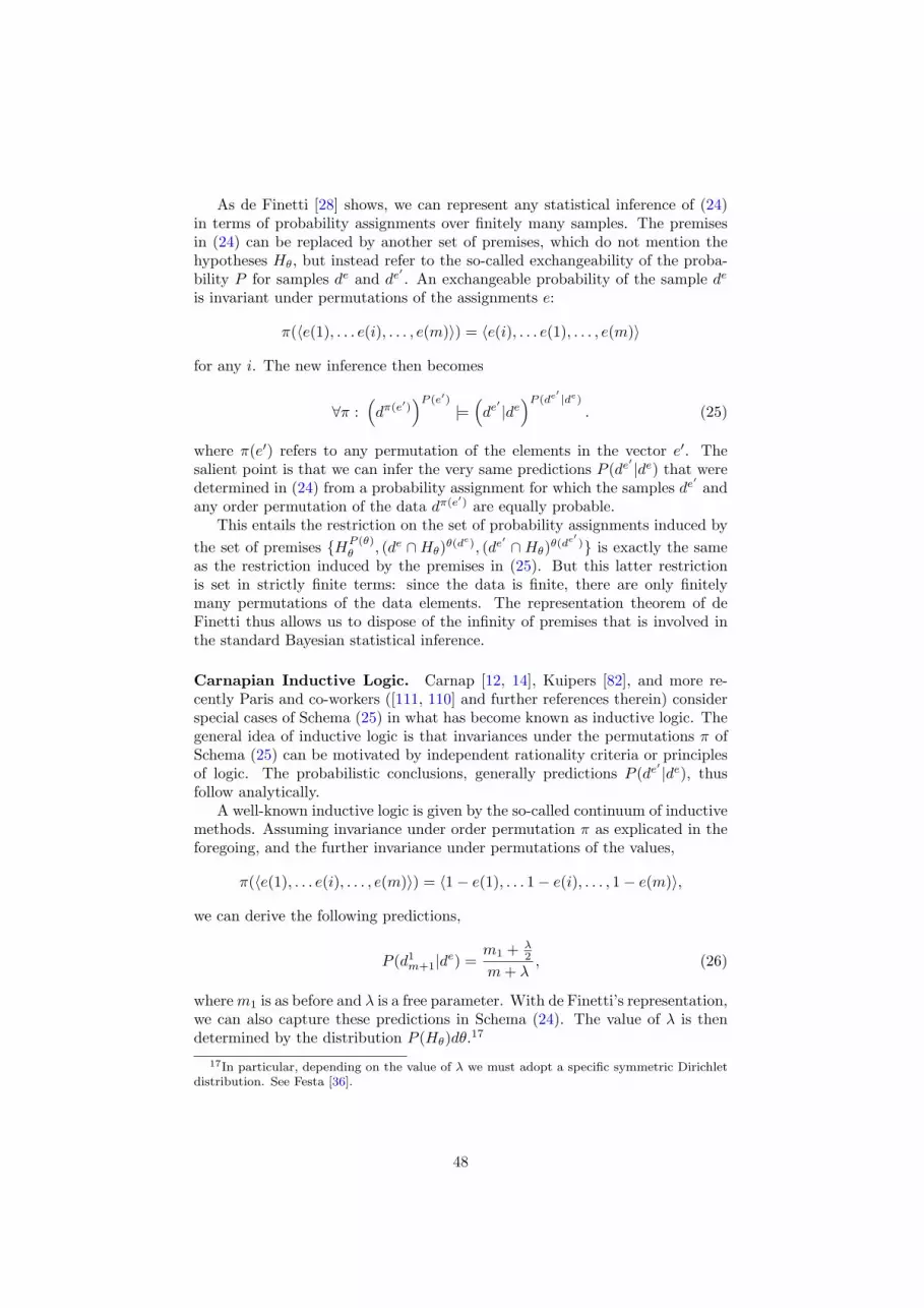
As de Finetti [28] shows, we can represent any statistical inference of (24)in terms of probability assignments over finitely many samples. The premisesin (24) can be replaced by another set of premises, which do not mention thehypotheses Hθ, but instead refer to the so-called exchangeability of the proba-bility P for samples de and de

′. An exchangeable probability of the sample de

is invariant under permutations of the assignments e:

π(〈e(1), . . . e(i), . . . , e(m)〉) = 〈e(i), . . . e(1), . . . , e(m)〉

for any i. The new inference then becomes

∀π :(dπ(e′)

)P (e′)

|=(de′ |de)P (de

′ |de). (25)

where π(e′) refers to any permutation of the elements in the vector e′. Thesalient point is that we can infer the very same predictions P (de

′ |de) that weredetermined in (24) from a probability assignment for which the samples de

′and

any order permutation of the data dπ(e′) are equally probable.This entails the restriction on the set of probability assignments induced by

the set of premises HP (θ)θ , (de ∩Hθ)θ(d

e), (de′ ∩Hθ)θ(d

e′ ) is exactly the sameas the restriction induced by the premises in (25). But this latter restrictionis set in strictly finite terms: since the data is finite, there are only finitelymany permutations of the data elements. The representation theorem of deFinetti thus allows us to dispose of the infinity of premises that is involved inthe standard Bayesian statistical inference.

Carnapian Inductive Logic. Carnap [12, 14], Kuipers [82], and more re-cently Paris and co-workers ([111, 110] and further references therein) considerspecial cases of Schema (25) in what has become known as inductive logic. Thegeneral idea of inductive logic is that invariances under the permutations π ofSchema (25) can be motivated by independent rationality criteria or principlesof logic. The probabilistic conclusions, generally predictions P (de

′ |de), thusfollow analytically.

A well-known inductive logic is given by the so-called continuum of inductivemethods. Assuming invariance under order permutation π as explicated in theforegoing, and the further invariance under permutations of the values,

π(〈e(1), . . . e(i), . . . , e(m)〉) = 〈1− e(1), . . . 1− e(i), . . . , 1− e(m)〉,

we can derive the following predictions,

P (d1m+1|de) =

m1 + λ2

m+ λ, (26)

wherem1 is as before and λ is a free parameter. With de Finetti’s representation,we can also capture these predictions in Schema (24). The value of λ is thendetermined by the distribution P (Hθ)dθ.17

17In particular, depending on the value of λ we must adopt a specific symmetric Dirichletdistribution. See Festa [36].

48

6.2.2 Interval-Valued Priors and Posteriors

Until now we have focused on sets of probability assignments that can be definedby restrictions in terms of sharp probability assignments. But we may also rep-resent restrictions in terms of intervals of probability assignments. We can usethis to represent a wider class of Bayesian statistical inferences in Schema (1).

Walley [101] discusses interval restrictions in the context of the above multi-nomial hypotheses and their associated Carnapian predictions. As said, a sharpdistribution over multinomial hypotheses leads to an exchangeable predictionrule. Walley points out that we can also allow for interval-valued assignments tostatistical hypotheses, and that such valuations can be dealt with adequately byconsidering a class of prior distributions over the statistical hypotheses insteadof a single and sharp-valued prior distribution. These interval-valued assign-ments are useful in studying the sensitivity of statistical results to the priorprobability that is chosen.

Furthermore, classes of prior distributions are associated with ranges of pre-diction rules. As Skyrms [132] and Festa [37] show, we can use such ranges ofrules to constitute so-called hyper-Carnapian prediction rules: each of the theprediction rules reacts to the incoming sample separately, but each predictionrule is also assigned a probability, and the probability assignment over the rulesis updated according to the data as well. The resulting prediction rules havequite interesting properties. Most notably, they can be used for deriving pre-dictions that incorporate analogical predictions. However, it is not easy, nor isit in our opinion very insightful, to represent the higher-order probability as-signments over Carnapian rules in terms of the scheme of Schema (1). In thispaper we will therefore not study the hyper-Carnapian prediction rules.

6.3 Interpretation

We can interpret Schema (1) straightforwardly as a Bayesian statistical infer-ence, as long as the inference concerns probability assignments over a samplespace and a model, ΩD × ΩH . One type of premise concerns the data andthe statistical model: we restrict ourselves to those probability assignments forwhich the likelihoods of the hypotheses on the data, P (D|Hj), have specific val-ues. The other premise is the prior probability assignment: we restrict the setof probability assignments to those for which the marginal probability over hy-potheses P (Hj) is equal to specific values. From these two restrictions and theassignment d to the data variable D we can derive, according to the progicnetprogramme, a further restriction on the posterior probability P (Hj |d).

6.3.1 Interpretation of Probabilities

Bayesian statistics is very often associateed with the so-called subjective inter-pretation of probability. Thus far we have not determined the interpretationof the probability assignments featuring in the inference. We want to brieflycomment on the issue of interpreting probability here.

First, as probabilistic logicians we are not necessarily tied to a specific inter-pretation of the probability functions, just like classical deductive logicians arenot necessarily tied to Tarski’s or some other truth definition as an interpreta-tion of the truth values in their inferential schemes. This is fortunate, because

49

the debate on interpretations of probability is very complicated, and it easilymuddles the discussion on probabilistic inference, especially Bayesian inference.On the whole, our present concerns are not with these interpretative issues, butwith the logic and its formal semantics.

If we are interpreting probabilities, we should distinguish between the prob-ability assigned to statistical hypotheses Hj and to samples or data d. Withregard to the former, note that the schema concerns statistical hypotheses intwo ways: on the one hand the hypotheses are expressions in the language, onthe other hand they determine a probability assignment over the language. Nowin a standard Bayesian account, probability assignments over hypotheses seemmost naturally understood as epistemic, meaning that they pertain to degreesof belief. Note that this does not yet mean that probabilities of hypothesesare subjective, because we may also try to determine the epistemic probabilityassignment by means of objective criteria.

As for the probability assigned to samples, the likelihoods, we may give iteither a physical interpretation, meaning that the probabilities refer to aspectsof the physical world, or an epistemic interpretation. Arguably, the probabilityassignments as prescribed by the hypotheses are best interpreted as a physicalnotion, because hypotheses are statements about the world. At the same timethe likelihoods of the hypotheses seem best interpreted as epistemic, becausethey fulfill an evidential role.

6.3.2 Bayesian confidence intervals

There is another, rather natural interpretation of interval probabilities in thecontext of Bayesian statistical inference. We discuss it briefly here to clarify itsrelation to Schema (1), and to explain why we will not pursue this interpretationin what follows.

Recall that the continuum of hypotheses Hθ concerns probability assign-ments over data D via the parameter θ, and that we have defined probabilitydensity functions over this parameter, P (Hθ|D). From these density functionswe can define Bayesian confidence intervals, or credence intervals, for the val-ues of θ. Each interval θ ∈ [l, u] is associated with a posterior probability, orcredence,

P (h[l,u]|D) =∫ u

l

P (Hθ|D)dθ.

Now we may fix u and l such that

∫ l

0

P (Hθ|D)dθ =∫ 1

u

P (Hθ|D)dθ = 2.5%.

In that case we have P (h[l,u]|D) = 0.95, and we can then say that we are 95%certain that the real value of θ lies within the interval [l, u]. From the knowledgeof a sharp-valued probability assignment over θ, we might even construct aninterval-valued probability assignments for θ, written θ ∈ [l, u].

Credence intervals might lead us to reconsider the representation of theBayesian statistical inferences in Scheme (22), and bring Bayesian statisticalinference closer to classical statistical inference. Assuming a uniform priorprobability density P (Hθ) = 1, the corresponding interval-valued assignmentis θ ∈ [.025, .975]. But after incorporating a specific sample d, we obtain the

50

posterior density function P (Hθ|d). It may so happen that the correspondinginterval-valued assignment is θ ∈ [.08, .13], meaning that conditional on obtain-ing the data d, the 95% credence interval shrinks. The question arises whetherwe can somehow interpret the interval-valued probabilities in Schema (1) assuch credence intervals.

Unfortunately, we cannot. The inferences of interval-valued probabilities inSchema (1), when interpreted as credence intervals, are elliptic, that is, theyomit certain premises. More precisely, the fact that θ ∈ [.025, .975] does notfix the detailed shape of the prior probability density P (Hθ). But we need thisdetailed shape to arrive at the specific conditional credence interval θ ∈ [.08, .13].It is not possible to rely just on the rules of inference of Schema (1) for thesecredence intervals. An interpretation of Schema (1) in terms of the credenceintervals deriving from Bayesian statistical inference is therefore not possible.

7 Objective Bayesianism

7.1 Background

According to objective Bayesian epistemology, an agent’s rational degrees ofbelief are determined by the extent and limitations of the propositions E that shetakes for granted [155]. E is called the agent’s epistemic background , or evidence,and includes her background knowledge, observations, theoretical assumptionsetc.—everything that is not under question in her current operating context.The agent’s epistemic background determines the strengths of the her beliefsin two ways. First, an agent’s degrees of belief should be compatible with thisbackground: e.g., if she grants ϕ, she should fully believe it; if her evidenceconsists just of a narrowest reference-class frequency pertinent to ϕ then sheshould believe it to the extent of that frequency; if her granted physical theorydetermines the chance of ϕ then she should believe it to the extent of thatchance; if her granted physical theory says that there is a symmetry betweenϕ and ϕ′ which results in them having the same chance then she should awardthem the same degree of belief.18 Second, her degrees of belief should otherwisebe as equivocal as possible—she should not believe a proposition to a greateror lesser extent than the most equivocal degree of belief that is compatible withher epistemic background.

7.1.1 Determining Objective Bayesian Degrees of Belief

Importantly, objective Bayesianism—in common with other versions of Bayesianepistemology—holds that the agent’s rational degrees of belief are representableby a probability function; thus her degree of belief in ϕ can be measured by asingle number in the unit interval. This position can be motivated by bettingconsiderations [118, 27] or by derivation from intuitive principles [17]. ManyBayesians also agree with the objective Bayesian tenet that the agent’s proba-

18For an agent’s degrees of belief to be rational, it is sufficient that they be rationallydetermined from her background E, that this background consists of propositions that theagent takes for granted, and that the agent is rational to take these propositions for grantedgiven her purposes at the time. The truth of the propositions in E is not required. Hence thepropositions in E need count as knowledge in the philosophical sense that presupposes truth.

51

bility function should satisfy constraints imposed by E .19 The motivation behindthis tenet is that an agent’s degrees of belief will be used as a basis for inferenceand decision; success in these tasks require calibration with physical probability.

What separates objective Bayesianism from other varieties of Bayesianism isits further insistence on equivocal degrees of belief: an agent’s probability func-tion should be a probability function, from those satisfying constraints imposedby background knowledge, that is as non-extreme as possible. This is becauseextreme degrees of belief tend to trigger risky actions while equivocal degreesof belief are associated with less risk, and it is prudent only to take on risk tothe minimum extent warranted by available evidence [152].

The general recipe for objective Bayesian assignment of belief proceeds asfollows. The epistemic background E determines a set E of probability functionswhich are compatible with E . The agent should then have degrees of belief thatare representable by a probability function PE which is in E and as close aspossible to an equivocator , a probability function P= that is maximally equivocalon the domain. To flesh out this procedure, we need to say a bit more about howE is determined by E , and more precisely characterise the notions of equivocatorand closeness to the equivocator.

7.1.2 Constraints on Degrees of Belief

First we shall say a few words about how E is determined by E . The idea hereis that E imposes constraints χ that an agent’s degrees of belief should satisfy.This set of constraints can be used to characterise E, the set of probabilityfunctions that are compatible with E .

Definition 7.1 (Directly Transferred Constraints) The set of directly trans-ferred constraints is the smallest set χ such that:

• if ϕ is in E then P (ϕ) = 1 is in χ,

• if chance(ϕ) ∈ X is in E then P (ϕ) ∈ X is in χ (more generally, substituteP for chance when transferring constraints to χ),

• if freqU (V ) ' x (which says ‘the frequency of V in reference class U isapproximately x’) is in E and V t↔ ϕ is in E and Ut ∈ E and there is nonarrower U ′ for which this holds, then P (ϕ) = x is in χ (more generally,let known narrowest-reference-class frequencies transfer to constraints onP in χ).20

Let P be the set of all probability functions and let Pχ be the set of probabilityfunctions that satisfy χ, the directly transferred constraints. There are tworeasons why we can’t just set E = Pχ. First, it is sometimes unreasonable torequire that degrees of belief should satisfy the same constraints as physicalprobabilities (frequencies, chances). For example, suppose the agent knows justthat the truth of ϕ has already been decided (ϕ asserts the occurrence of an event

19Some Bayesians restrict this to the case in which the knowledge in a takes the form ofsentences in the domain of the probability function (in which case the constraints are usuallyjust that these sentences should be fully believed). The objective Bayesian does not imposethis restriction.

20Depending on the closeness of the approximation freqU (V ) ' x (e.g., depending on thesample size) one might relax this constraint to P (ϕ) = [x− δ, x+ δ] for some suitable δ.

52

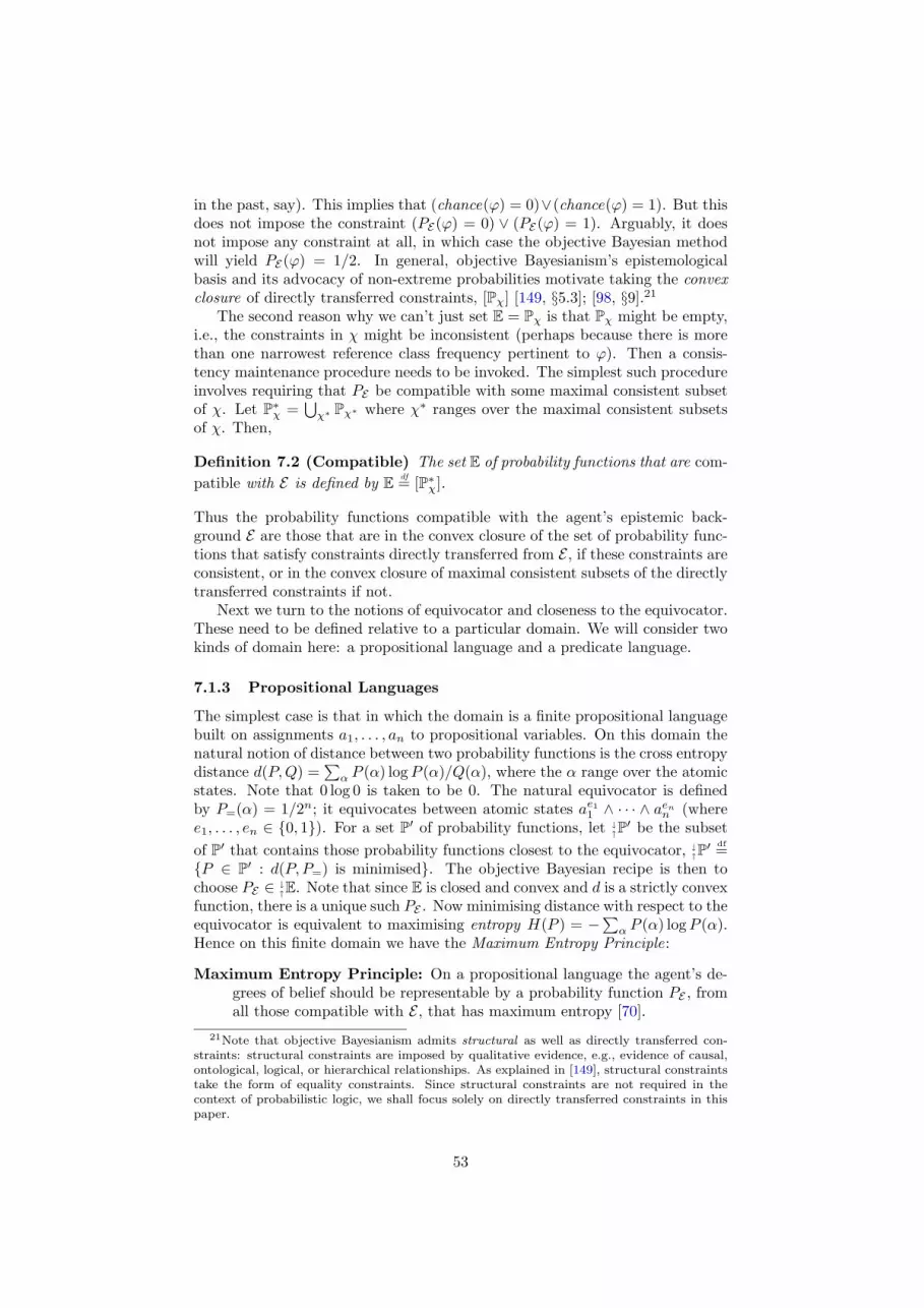
in the past, say). This implies that (chance(ϕ) = 0)∨(chance(ϕ) = 1). But thisdoes not impose the constraint (PE(ϕ) = 0) ∨ (PE(ϕ) = 1). Arguably, it doesnot impose any constraint at all, in which case the objective Bayesian methodwill yield PE(ϕ) = 1/2. In general, objective Bayesianism’s epistemologicalbasis and its advocacy of non-extreme probabilities motivate taking the convexclosure of directly transferred constraints, [Pχ] [149, §5.3]; [98, §9].21

The second reason why we can’t just set E = Pχ is that Pχ might be empty,i.e., the constraints in χ might be inconsistent (perhaps because there is morethan one narrowest reference class frequency pertinent to ϕ). Then a consis-tency maintenance procedure needs to be invoked. The simplest such procedureinvolves requiring that PE be compatible with some maximal consistent subsetof χ. Let P∗χ =

⋃χ∗ Pχ∗ where χ∗ ranges over the maximal consistent subsets

of χ. Then,

Definition 7.2 (Compatible) The set E of probability functions that are com-patible with E is defined by E df= [P∗χ].

Thus the probability functions compatible with the agent’s epistemic back-ground E are those that are in the convex closure of the set of probability func-tions that satisfy constraints directly transferred from E , if these constraints areconsistent, or in the convex closure of maximal consistent subsets of the directlytransferred constraints if not.

Next we turn to the notions of equivocator and closeness to the equivocator.These need to be defined relative to a particular domain. We will consider twokinds of domain here: a propositional language and a predicate language.

7.1.3 Propositional Languages

The simplest case is that in which the domain is a finite propositional languagebuilt on assignments a1, . . . , an to propositional variables. On this domain thenatural notion of distance between two probability functions is the cross entropydistance d(P,Q) =

∑α P (α) logP (α)/Q(α), where the α range over the atomic

states. Note that 0 log 0 is taken to be 0. The natural equivocator is definedby P=(α) = 1/2n; it equivocates between atomic states ae11 ∧ · · · ∧ aenn (wheree1, . . . , en ∈ 0, 1). For a set P′ of probability functions, let ↓↑P′ be the subsetof P′ that contains those probability functions closest to the equivocator, ↓↑P′

df=P ∈ P′ : d(P, P=) is minimised. The objective Bayesian recipe is then tochoose PE ∈ ↓↑E. Note that since E is closed and convex and d is a strictly convexfunction, there is a unique such PE . Now minimising distance with respect to theequivocator is equivalent to maximising entropy H(P ) = −∑α P (α) logP (α).Hence on this finite domain we have the Maximum Entropy Principle:

Maximum Entropy Principle: On a propositional language the agent’s de-grees of belief should be representable by a probability function PE , fromall those compatible with E , that has maximum entropy [70].

21Note that objective Bayesianism admits structural as well as directly transferred con-straints: structural constraints are imposed by qualitative evidence, e.g., evidence of causal,ontological, logical, or hierarchical relationships. As explained in [149], structural constraintstake the form of equality constraints. Since structural constraints are not required in thecontext of probabilistic logic, we shall focus solely on directly transferred constraints in thispaper.

53

7.1.4 Predicate Languages

If the domain is a predicate language then the picture is similar, but slightlymore complicated.22 In this case we create an ordering a1, a2, . . . of the atomicsentences—sentences of the form Ut where U is a predicate or relation and t is atuple of constants of corresponding arity—ensuring that those atomic sentencesthat only involve constant symbols from t1, . . . , tm occur in the ordering beforethose that involve tn, for m < n. We then use as the measure of distance

dn(P,Q) df=1∑

e1,...,en=0

P (ae11 ∧ · · · ∧ aenn ) logP (ae11 ∧ · · · ∧ aenn )Q(ae11 ∧ · · · ∧ aenn )

.

Here, as before, a1i signifies ai and a0

i signifies ¬ai. As before we take 0 log 0 tobe 0. We will not need to consider the case x log x/0 and will simply assume inwhat follows that Q is never zero.

On a predicate language the equivocator is defined by

P=(ae11 ∧ · · · ∧ aenn ) df= 1/2n,

for all n. Thus

dn(P, P=) =1∑

e1,...,en=0

P (ae11 ∧ · · · ∧ aenn ) log [2nP (ae11 ∧ · · · ∧ aenn )] .

Letting d(P,Q) = limn→∞ dn(P,Q) ∈ [0,∞], one might try, as before, tochoose PE ∈ P ∈ E : d(P, P=) is minimised. But as it stands this does notadequately explicate the concept of closeness to the equivocator, because inthe case of a predicate language there are probability functions P,Q such thatalthough one is intuitively closer to the equivocator than the other, d(P, P=) =d(Q,P=). Suppose for example that E imposes the constraints P (an|ae11 ∧ · · · ∧aen−1n−1 ) = 1 for all n≥ 2. Thus only P (a1) is unconstrained. Then Pχ is non-

empty, closed and convex, so E = Pχ, but d(P, P=) = ∞ for all P ∈ E. Yetintuitively there is a unique function in E that is closest to the equivocator,namely the function that sets P (a1) = 1/2 and P (an|ae11 ∧ · · · ∧ a

en−1n−1 ) = 1 for

all n≥2. Accordingly we introduce the following definition.

Definition 7.3 (Closer) For probability functions P,Q,R defined on a predi-cate language, we say P is closer than Q to R iff there is some N such that forall n≥N , dn(P,R) < dn(Q,R).

Note that in the above example, the function that is intuitively closer to theequivocator is indeed deemed to be closer (N can be taken to be 1 in this case).Here is another example:

Example 7.4 Suppose E = P ∈ P : P (∀xUx) = c for some fixed c ∈[0, 1]. (It is usual to understand a constraint of the form P (∀xUx) = c as

22Note that the approach advocated here is very different to that of [151, 154]. The meritof this new approach is that it permits a uniform treatment of propositional and predicatelanguages. We assume, as is normal with discussions of probabilities over predicate languages,that each element of the domain is picked out by some constant symbol. See [111] on thispoint.

54

limn→∞ P (Ut1 ∧ · · · ∧ Utn) = c).23 We have that d(P, P=) = ∞ for all P ∈ E.Define P by

P (Ut1) =c+ 1

2

P (Uti+1|Ute11 ∧ · · · ∧ Uteii ) =

(2i+1−1)c+1(2i+1−2)c+2 : e1 = · · · = en = 1

12 : otherwise

Then P is the member of E that is closest to the equivocator.

The objective Bayesian protocol is then to seek a probability function thatis closest to the equivocator in the sense of Definition 7.3. For a set P′ ofprobability functions, let ↓↑P′ be those members of P′ that are closest to theequivocator P= in the sense of Definition 7.3. Then objective Bayesianismadvocates choosing PE ∈ ↓↑E, as in the case of a propositional language. (Whilein the propositional case PE is uniquely determined, this is not necessarily sowith a predicate language.)

The following objection to the above choice of equivocator crops up fromtime to time in the literature [31, §4]. Suppose the agent has no backgroundknowledge E ; then she will set her degrees of belief according to the equivocator.In particular P=(Br101 | Br1 ∧ · · · ∧ Br100) = P=(Br101) = 1/2. Thus if sheobserves a hundred ravens and finds them all to be black then her degree ofbelief that raven 101 will be black is the same as if she had observed no ravensat all. Learning from experience becomes impossible with this equivocator.

This objection fails because P=(Br101 | Br1∧· · ·∧Br100) does not representthe degree to which the agent would believe that raven 101 is black were sheto observed a hundred ravens all black. Suppose the agent’s initial epistemicbackground E = ∅; then indeed PE = P=. Suppose then the agent were toobserve a hundred ravens and find them all black. Her new epistemic backgroundis E ′ = Br1 ∧ · · · ∧ Br100. Her degree of belief that raven 101 is black giventhis evidence is PE′(Br101). This is obtained by determining the P ∈ PE′ thatis closest to P=. To determine PE′ we need to isolate the constraints imposedby E ′. Clearly E ′ imposes the constraint P (Br1 ∧ · · · ∧ Br100) = 1, but theevidence also implies that the relative frequency of ravens being black is near 1,so by Definition 7.1 also constrains P (Bri) to be near 1 for unobserved ri. NowPE′ must satisfy these constraints so PE′(Br101) will end up being near 1 (whichseems reasonable given the agent’s lack of other knowledge). Thus the agent willlearn from experience after all. More generally, the objective Bayesian updateon new evidence e does not always agree with the corresponding conditionalprobability PE(·|e). One of the conditions for agreement is that e be simplewith respect to previous knowledge E , i.e., that the learning of e should onlyimpose the constraint P (e) = 1. In this case, e contains frequency informationand so is not simple. See [153] for a fuller discussion of the differences betweenobjective Bayesian updating and Bayesian conditionalisation.

7.1.5 Objective Bayesianism in Perspective

We see, then, that objective Bayesianism requires that the strengths of anagent’s beliefs be representable by a probability function, from all those that are

23See [111] for instance. Note that this construal requires the assumption that each memberof the domain is picked out by some constant symbol in the language.

55

compatible with the propositions that she takes for granted, which is closest toa suitable equivocator on the domain. One can take much the same approachon both predicate and propositional languages.

Jakob Bernoulli may be have been the first to advocate all three of thecentral tenets of objective Bayesianism, namely that degrees of belief shouldbe probabilistic, constrained by empirical evidence, and otherwise equivocal [6,Part IV]; [149, §5.2]. [70] provided the maximum-entropy foundations whichwork well on finite domains; how to handle uncountable domains remains aquestion of some controversy [155, §19]. Uncountable domains are less centralto logic and to the purposes of this paper, and so will not be covered here. [109,§4] applied objective Bayesianism to probabilistic logic.

Objective Bayesianism as outlined here differs in an important sense fromBayesian statistical inference described in §6: here all probabilities are first-order, attaching to sentences of a logical language, while Bayesian statisticalinference focuses on second-order probabilities, i.e., probabilities of probabilities.Objective Bayesian statistical inference, which appeals to equivocal second-orderprobabilities, is an active research area in statistics. Objective Bayesianismdiffers from probabilistic argumentation (§3) inasmuch as it is concerned withthe probability that a conclusion is true, rather than the probability that theconclusion’s truth is forced by the truth of the premises. Evidential probability(§4) can be viewed as a formalism for determining E, the set of probabilityfunctions that are compatible with the agent’s epistemic background; objectiveBayesianism goes beyond evidential probability in that it advocates equivocationas well as calibration with statistical evidence [146].

7.2 Representation

The objective Bayesian faces the following kind of question: given backgroundknowledge E , to what extent should you believe a proposition ψ of interest?It is not hard to see how this might be phrased in terms of the Fundamen-tal Question of Probabilistic Logic, Equation 1. Suppose for instance thatE = ϕ1, chance(ϕ2) ∈ [0.6, 0.8], freqU (V ) ' 0.9, V t ↔ ϕ3, Ut.24 Then theobjective Bayesian question can be phrased in the language of Equation 1 asfollows:

ϕ11, ϕ

[0.6,0.8]2 , ϕ0.9

3 |≈ ψ?

Thus objective Bayesianism fits neatly into the framework of this paper.

7.3 Interpretation

Conversely, a question of the form of Equation 1, ϕX11 , ϕX2

2 , . . . , ϕXnn |≈ ψ?, canbe given an objective Bayesian interpretation. Simply take the premisses onthe left-hand side to encapsulate constraints on P that are directly transferredfrom an agent’s background knowledge (i.e., constraints in the set χ introducedabove). Then the set Y to attach to ψ is the set Y = PE(ψ) : PE is a functionfrom [P∗χ] that is closest to the equivocator. Assuming a finite domain, Y is asingleton.

24To reiterate, while the propositions ϕ1, ϕ2, ϕ3 are in the domain of the agent’s probabilityfunction, expressions of the form chance(ϕ2) ∈ [0.6, 0.8], freqU (V ) ' 0.9, V t↔ ϕ3, Ut are notassumed to be in this domain.

56

Thus objective Bayesianism can be used to provide semantics for probabilis-tic logic. Let χ = ϕX1

1 , ϕX22 , . . . , ϕXnn and let ν be ψY . Then χ |≈ ν if and

only if P ∈ ↓↑[P∗χ] implies P (ψ) ∈ Y , i.e., if and only if ↓↑[P∗χ] ⊆ Pν .

Example 7.5 Consider the question ∀xUx3/5 |≈ Ut?. Objective Bayesian epis-temology interprets the expression on the left-hand side as the constraint χ im-posed on an agent’s degrees of belief by her evidence E; this constraint is con-sistent and determines a closed convex set, so E = [P∗χ] = Pχ = P ∈ P :P (∀xUx) = 3/5. There is one function P in E that is closest to the equivo-cator, as described in Example 7.4. This function gives P (Ut) = 4/5 for eachconstant t. Hence the answer to the question is 4/5.

Note that the monotonicity property of §1.2 fails, so entailment is not decom-posable under the objective Bayesian semantics. Nevertheless, this notion ofentailment still satisfies a number of interesting properties. In order to charac-terise these properties we shall need to appeal to some notions that are commonin the literature on nonmonotonic logics—see, e.g., [81]; [102, §3.2] and [64] forbackground. Construct an (uncountable) language L∗ by taking statements ofthe form ϕX as atomic propositions, where ϕ is a sentence of a propositionalor predicate language L and X is a set of probabilities. L∗ can be thoughtof as the language of the Fundamental Question, Equation 1. A probabilityfunction P can then be construed as a valuation on L∗. Define a decomposableentailment relation |= by P |= µ iff P ∈ Pµ for sentence µ of L∗, where µ iscomposed from statements of the form ϕX by the usual logical operators. Inparticular, if µ is of the form ϕX , then P |= µ iff P (ϕ) ∈ X. For probabilityfunctions P and Q, define P ≺ Q iff P is closer to the equivocator than Q.Then (P,≺, |=) is a preferential model : P is a set of valuations on L∗, ≺ isan irreflexive, transitive relation over P, and |= is a decomposable entailmentrelation. Moreover, this preferential model is smooth: if P |= µ then either Pis minimal with respect to ≺ in Pµ or there is a Q ≺ P in Pµ that is minimal.Hence this model determines a preferential consequence relation |∼ as follows:µ |∼ ν iff P satisfies ν for every P ∈ P that is minimal among those probabilityfunctions that satisfy µ. We will be particularly interested in the case in whichsentence µ of L∗ is consistent and where all sets X occurring in µ are closedintervals. In that case Pµ = P∗µ = [P∗µ] = E, the set of probability functions thatare compatible with µ. Call µ regular if it satisfies this property. Wherever µand ν are regular sentences, |∼ will agree with |≈, where the latter entailmentrelation is extended to L∗ in the obvious way. Consequently on regular sen-tences |≈ will satisfy the properties of preferential consequence relations, oftencalled system-P properties—see, e.g., [81]:

Proposition 7.6 (Properties of Entailment) Let |= denote entailment inclassical logic and let ≡ denote classical logical equivalence. Whenever µ∧ξ, ν∧ξare regular sentences of L∗,Right Weakening: if µ |≈ ν and ν |= ξ then µ |≈ ξ.

Left Classical Equivalence: if µ |≈ ν and µ ≡ ξ then ξ |≈ ν.

Cautious Monotony: if µ |≈ ν and µ |≈ ξ then µ ∧ ξ |≈ ν.

Premiss Disjunction: if µ |≈ ν and ξ |≈ ν then µ ∨ ξ |≈ ν.

57

Conclusion Conjunction: if µ |≈ ν and µ |≈ ξ then µ |≈ ν ∧ ξ.

The objective Bayesian semantics is sometimes preferred to the standardsemantics on conceptual grounds (semantics in terms of rational degrees of beliefis very natural, and objective Bayesianism provides a compelling account ofrational degree of belief) and sometimes on pragmatic grounds—that a singleprobability rather than a set of probabilities attaches to the conclusion of thefundamental question is computationally appealing and can simplify matters ifa decision must made on the basis of an answer to such a question [152, §11].

Part II

Probabilistic Networks

8 Credal and Bayesian Networks

In Part I we argued that the question of Schema (1), ϕX11 , . . . , ϕXnn |≈ ψ?, pro-

vides a unifying framework for probabilistic logic, into which several importantapproaches to probabilistic inference slot. Now, in Part II, we turn to the prob-lem of how one might answer this fundamental question.

We have seen that in many cases it suffices to restrict attention to convex setsof probability functions, and even, in the case of objective Bayesianism, often asingle probability function. This restriction will be important in what follows,since it will allow us to exploit the computational machinery of probabilisticnetworks—in particular credal networks and Bayesian networks—to help usanswer the fundamental question.

The task, then, is to find an appropriate Y such that ϕX11 , . . . , ϕXnn |≈ ψY ,

where X1, . . . , Xn, Y are intervals of probabilities. Our strategy is to use the lefthand side, ϕX1

1 , . . . ϕXnn , to determine a probabilistic network on the domain.This probabilistic network offers an efficient means of representing the proba-bility functions that are models of the left hand side, and an efficient meansof drawing inferences from these probability functions. One can then use thisnetwork to calculate Y , the range of probability values that models of the lefthand side attach to ψ.

In §8.1 we introduce credal and Bayesian networks and the different config-urations of these networks that will be required in Part II of this paper. Then,in §8.2, we develop some common machinery for drawing inferences from prob-abilistic networks in order to answer our fundamental question. The remainderof Part II will be devoted to exploring the variety of networks produced bythe different semantics of Part I. In each subsequent section we shall provideone or more algorithms for constructing a probabilistic network that suits thecorresponding semantics. We will focus on explaining the basic steps of eachconstruction algorithm in broad terms. Space constraints prohibit detailed anal-ysis and justification of these algorithms but further details are available in thesupporting references. In summary, then, the recipe of this paper is as follows:

• Representation: Formulate a question of the form of Schema (1).

• Interpretation: Decide upon appropriate semantics (Part I).

58

• Network Construction: Construct a probabilistic network to representthe models of the left-hand side of Schema (1) (subsequent sections ofPart II).

• Inference: Apply the common machinery of §8.2 to answer the questionposed in the first step.

This paper is by no means the first to advocate integrating probabilisticlogics and probabilistic networks [see, e.g., 116, 108, 69, 75, 119, 92, 93, 18].Previous work has focussed on developing specific probabilistic logics that inte-grate probabilistic networks into the representation scheme—i.e., into the logi-cal syntax itself. Here, however, we adopt a quite different approach, by usingprobabilistic networks as a calculus for probabilistic logic in general. Thus prob-abilistic networks play a role here analogous to that of proof in classical logic:they provide a means of answering the kind of question that the logic faces.

8.1 Kinds of Probabilistic Network

Suppose we have a finite propositional language LV with propositional variablesV = A1, . . . , An which may take values true or false. As outlined in §1.4, theassignment Ai = true is denoted by a1

i or simply ai, while Ai = false is denotedby a0

i or ai. A Bayesian network consists of a directed acyclic graph (DAG) onV , together with the probability functions P (Ai|PARi) for each variable Ai ∈ Vconditional on its parents PARi ⊆ V in the graph. (Here P (aei |parei ) refers tothe probability of a particular assignment to variable Ai conditional on the prob-ability of a particular assignment to its parents, while P (Ai|PARi) refers to theprobability function itself—i.e., the function that maps assignments to Ai andits parents to numbers in the unit interval.) An example of a Bayesian network

A1 A2 A3

Figure 5: Directed acyclic graph in a Bayesian network.

is provided by the graph of Figure 5 together with corresponding conditionalprobability functions specified by:

P (a1) = 0.1, P (a2|a1) = 0.9, P (a3|a2) = 0.4,P (a2|a1) = 0.3, P (a3|a2) = 0.2.

The joint probability function P over LV is assumed to satisfy the Markovcondition: each variable is probabilistically independent of it’s non-descendantsND i conditional on its parents PARi, written Ai ⊥⊥ ND i|PARi. Under this as-sumption, a Bayesian network suffices to determine the joint probability functionunder the identity

P (A1, . . . , An) =n∏

i=1

P (Ai|PARi). (27)

In the above example,

P (a1a2a3) = P (a3|a2)P (a2|a1)P (a1) = 0.2× (1− 0.9)× 0.1 = 0.002.

59

A credal network consists of a directed acyclic graph on V = A1, . . . , Antogether with closed convex sets K(Ai|PARi) of conditional probability func-tions P (Ai|PARi), for each variable Ai ∈ V conditional on its parents in thegraph. As previously mentioned, a closed convex set of probability functionsis called a credal set . (See §2.1.4 for more on convexity.) As an example of acredal network consider Figure 5 together with the local conditional distribu-tions constrained by

P (a1) ∈ [0.1, 0.2], P (a2|a1) = 0.9, P (a3|a2) ∈ [0.4, 1],P (a2|a1) ∈ [0.3, 0.4], P (a3|a2) = 0.2.

8.1.1 Extensions

In a credal network, further independence assumptions are made in order todetermine a joint credal set K(A1, . . . , An) over the whole domain from thegiven conditional credal sets. The credal network framework admits a numberof choices as to which assumptions to make here.

Natural Extension. One choice is to make no independence assumptions atall. Then we have what in [19] is called a natural extension under noconstraints, i.e., the joint credal set

K(A1, . . . , An) = P : P (Ai|PARi) ∈ K(Ai|PARi),

whose elements all comply with the probabilistic constraints of the givenconditional credal sets.

Strong Extension. Another possible choice is to take the convex hull of theextremal points defined by the local conditional credal sets and the con-ditional independencies determined from the graph via the Markov con-dition. The resulting joint credal set, is then called the strong extensionof the credal network. It is noteworthy that not all probability assign-ments in the strong extension need comply with the independence rela-tions suggested by the graph—only the extremal points need satisfy thesecontraints. This is further explained in §8.1.2 below.

Complete Extension. Yet another choice is to assume that each probabilityfunction in the joint credal set satisfies the Markov condition with respectto the given graph. In that case the credal network can be thought of asthe set of Bayesian networks based on the given DAG whose conditionalprobabilities satisfy the constraints imposed by the conditional credal sets,P (Ai|PARi) ∈ K(Ai|PARi). We call the resulting credal set the completeextension of the credal network.25

Note that the natural extension coincides with the strong (or complete) exten-sion with respect to a complete graph (a DAG in which each pair of variablesis linked by an arrow, and which therefore implies no independencies via theMarkov condition). Hence it suffices to consider strong and complete extensions,and we will not appeal to the concept of natural extension in what follows. (Our

25A credal set is a closed convex set of probability functions. Convexity, however, is relativeto coordinate system; the complete extension is convex with respect to the network-structurecoordinate system. See §8.1.2 for further explanation.

60

discussion of the standard semantics and Bayesian statistical inference appealsto complete extensions, while strong extensions apply to objective Bayesian-ism.) Note too that the extremal points are independent of extension (i.e., theextremal points of any one extension coincide with those of any other exten-sion). In fact the inferences drawn from a credal network just depend on theseextremal points. Our common inferential machinery will handle the extremalpoints and so may be applied to any of the above extensions.

8.1.2 Extensions and Coordinates

The notion of extension is tied up with the notion of convexity. In §2.1.4 wenoted that whether or not a set of probability functions is convex depends onthe coordinate system used to specify the probability functions. In particular,depending on the choice of the coordinates for the space of probability functions,the strong extension of a network may be identical to the complete extension.We illustrate this with an example.

Example 8.1 Consider the credal network on variables A and B defined by theempty graph (no arrow between A and B) and local credal sets P (a) ∈ [0.3, 0.7],P (b) ∈ [0, 0.5]. This credal network defines four extremal points, each repre-sentable by a Bayesian network on the empty graph (implying via the Markovcondition that A ⊥⊥ B): one has local distributions P (a) = 0.3, P (b) = 0, asecond has P (a) = 0.7, P (b) = 0, the third P (a) = 0.3, P (b) = 0.5 and thefourth P (a) = 0.7, P (b) = 0.5. The strong extension of this credal network issimply the convex hull of these four extremal points.

But now the question arises as to how the convex hull in the above example isdefined. The convex hull of a set P of probability functions is the smallest set ofprobability functions that contains P and is closed under convex combination.A convex combination of functions P and Q is a function R such that z =λx+ (1− λ)y for each coordinate z of R, where x and y are the correspondingcoordinates of P and Q respectively and λ ∈ [0, 1].

One possibility is to specify a full joint distribution over the four atomicstates a∧ b, a∧¬b, ¬a∧ b, and ¬a∧¬b, and take as coordinates x1 = P (a∧ b),x2 = P (a∧¬b), x3 = P (¬a∧ b), and x4 = P (¬a∧¬b). We represent these fourmutually exclusive, exhaustive possibilities within a 3-dimensional unit simplexin Figure 6. Here the points where A and B are not dependent are those onthe curved surface. The small quadilateral on the curved surface identifies thepoints where A and B are independent from one another and satisfy the givenconstraints on assignments.

This curved surface is also depicted on the left hand side of Figure 7. Notethat it is not the case that all points in the convex hull of the small quadrilateralalso lie on the curved surface: the dotted line on the left hand side of Figure 7lies outside the surface. Hence probability functions within the strong extensionfail to satisfy the independence relation A ⊥⊥ B that is satisfied by the extremalpoints.

One can depict the full distribution over four possibilities using differentcoordinates. Now represent a probability function by coordinates α = P (a) =1 − P (a), β1 = P (b|a) = 1 − P (b|a), and β0 = P (b|a) = 1 − P (b|a). Thiscoordinate system is depicted by the cube on the right hand side of Figure 7.

61

P (a ! b)

P (a ! ¬b)

P (¬a ! b)

P (¬a ! ¬b)

P (a) ! [0.3, 0.7]

P (b) ! [0, 0.5]

Figure 6: Atomic-state coordinates.

Here A and B are independent, A ⊥⊥ B, iff β0 = β1. This is a linear restrictionin the space of possible assignments to A and B—the diagonal plane in thecube, which corresponds to the curved surface in the coordinate system on theleft hand side of Figure 7.

P (a ! b) P (a ! ¬b)

P (¬a ! b)

!!

!1 !

!0!

!

Figure 7: Two different coordinate systems.

Again, the small quadrilateral represents the region satisfying the constraintsimposed by the local credal sets. In this case, the convex hull of the extremalpoints of this region lies on the diagonal surface: all probability functions inthe strong extension satisfy the independence relation imposed by the graph inthe credal network, and hence the strong extension coincides with the completeextension.

This shows that the strong extension can depend on the coordinate systemused to represent probability functions. Hence it is important when using astrong extension to specify the coordinate system. In probabilistic logic it istypical to use the former, atomic-state coordinate system (x1, x2, x3, x4). Thisensures that if the extremal points all satisfy a linear constraint of the formP (ϕ) ∈ X then so will every member of the strong extension. (For example,the objective Bayesian semantics of §7 appeals to the atomic-state coordinatesystem in determining the convex closure of the probability function that satisfy

62

constraints imposed by evidence.) On the other hand, the latter, network-structure coordinate system (α, β0, β1) is often typical in discussions of causality,where it is more important that the strong extension preserve independencerelations than linear constraints.

8.1.3 Parameterised Credal Networks

It is important to note that there are credal sets that cannot be represented bya credal network of the above form.

Example 8.2 Consider the credal set that consists of all probability functionson V = A,B that satisfy the constraints P (ab) = 0.3 and P (b|a) = 0. Thisimplies P (a) ∈ [0.3, 1], but the possible values of P (b|a) depend on the particularvalue x of P (a) in [0.3, 1], since P (b|a) = 0.3/x. While it is true that P (b|a) ∈[0.3, 1], the value of P (b|a) can not be chosen independently of that of P (a). Sothe credal network defined on the graph with an arrow from A to B that has localcredal sets P (a) ∈ [0.3, 1], P (b|a) ∈ [0.3, 1], and P (b|a) = 0 does not representthe joint credal set. Note that the graph is complete so the choice of extensionis irrelevant here.

To represent the credal set of the above example we need to appeal to whatwe call a parameterised credal network . The graph is as before but now theconditional credal sets involve a parameter: x := P (a) ∈ [0.3, 1], P (b|a) = 0.3/x,and P (b|a) = 0. By invoking the parameter x, one avoids the assumption thatthe local credal sets operate independently as constraints on P . Parameterisedcredal networks can be used to represent arbitrary credal sets.

8.2 Algorithms for Probabilistic Networks

There has been a tremendous amount of research directed at finding the mostefficient algorithms for inference in Bayesian and credal networks. Nearly allcutting-edge algorithms for Bayesian networks use some sort of local computa-tion techniques [78, 94, 131], which try to systematically bypass operations onlarge state spaces. In the worst-case, these algorithms run in time and spaceexponential to the network’s induced treewidth, which is an indicator of the“density” of the available independence assumptions. Further improvements areobtained by exploiting so-called context-specific independencies [7, 140]. Thesetechniques deal with local independence relations within (rather than between)the given conditional probability tables.

In the case of credal networks, finding efficient inference algorithms is muchmore challenging. There are some attempts to apply local computation tech-niques to credal networks, but the problem remains unfeasible for most non-trivial instances. Compared to Bayesian networks, the additional computationalcomplexity results from the potentially unbounded number of extremal pointsneeded to describe arbitrary credal sets, which can quickly undermine any ben-efits of local computation. In fact, one can see inference in credal networks asa global multilinear optimization problem on top of the given network struc-ture [20], which is intractable on its own. Facing this inherent computationalcomplexity, exact inference methods are only exceptionally applicable to credalnetworks, and this is the reason why most of the current research in this areaaims at approximating the results rather than computing them precisely—see

63

[3, 9, 10, 51, 21, 22, 67, 68]. What is common to those methods is a generaldistinction between inner and outer approximations, depending on whether theapproximated interval is enclosed in the exact solution or vice versa.

In the remainder of this subsection, our goal is to single out an algorithmfor probabilistic networks which satisfies the particular requirements imposedby the framework of this paper. In the following sections, we shall then explorethe network construction problem for each of the proposed semantics.

8.2.1 Requirements of the Probabilistic Logic Framework

Despite the huge number of available algorithms for probabilistic networks, onlya few are valuable candidates for solving problems of the form of Schema (1).One reason for this is the fact that nearly all proposed semantics for probabilis-tic logic deal with sets of probabilities and are thus inherently tied to credalnetworks. In other words, inference algorithms for Bayesian networks are notgeneral enough to solve instances of Schema (1). Another reason hinges onthe following particular requirements, which are usually not of primary concernwhen building algorithms for probabilistic networks:

• Given that the conclusion ψ on the right hand side of Schema (1) may bean arbitrary logical formula, the algorithm must be able to compute prob-abilities P (ψ) or respective intervals [P (ψ), P (ψ)] of arbitrarily complexqueries. If ψ is a propositional formula, a general strategy to handle suchsituations is to decompose ψ into pairwise disjoint terms, thus producingwhat is called a disjoint sum-of-products. This can be done in two steps:first transform ψ into a disjunctive normal form (by applying de Morgan’slaws), and then apply Abraham’s algorithm to obtain ψ ≡ ψ1 ∨ · · · ∨ ψr,where each ψi is a conjunction of literals (term) satisfying ψi ∧ ψj ≡ ⊥for all j 6= i [1, 2]. This particular representation of ψ can then be usedto compute P (ψ) =

∑ri=1 P (ψi) as a sum of probabilities P (ψi), each of

them involving a simple term ψi only. The problem of computing proba-bilities of complex queries is thus reducible to the problem of computingterm probabilities, and the problem could be solved by querying the net-work r times, once for each individual term. But what we would ideallyexpect from an algorithm is the ability to compute such term probabilitiessimultaneously.

• Given that the premises on the left hand side of Schema (1) may includefunctionally interrelated probability intervals, e.g., to express conditionalindependencies (see §2.2), we would expect an algorithm to cope withthe parameters involved in the description of those interrelated intervals.In other words, what we need is a general machinery for parameterisedcredal networks. Following the remarks of §8.1.3, we assume linearity withrespect to the chosen coordinate system, in order to ensure that extremalpoints are easily identifiable.

The method sketched in the remainder of this section is a candidate for commoninferential machinery for various probabilistic logics. The core of the method hasoriginally been proposed as an exact inference algorithm for Bayesian networks[15, 16, 23, 139], but it is extensible to approximate inference in credal networks[51]. As we will see, it can also be used to simultaneously deal with multiple

64

queries and to handle functionally interrelated probability intervals, i.e., it meetsall the above requirements.

8.2.2 Compiling Probabilistic Networks

The general idea of compiling a probabilistic network is to split up inference intoan expensive compilation phase and a cheap query answering phase. For a givennetwork, the foregoing compilation phase is a unique step, which may take placewell before the actual inferences need to be conducted. Computationally, thecompilation may be very expensive, but once the compiled network is available,it is guaranteed that all sorts of probabilistic queries can be answered efficiently.

To implement this simple idea, the first step is to represent the topologicalstructure of a probabilistic network by propositional sentences. The resultingpropositional encoding of the network is then transformed into a generic graph-ical representation called deterministic, decomposable negation normal form, orsimply d-DNNF [24, 138]. One can think of a d-DNNF as a directed acyclicgraph whose internal nodes represent logical AND’s and OR’s, while the leavesat the bottom of the graph represent literals in a propositional language. Theinternal nodes are such that the children of an AND-node do not share commonvariables (called decomposability) and the children of an OR-node are pairwiselogically inconsistent (called determinism). These properties are crucial to con-duct probability computations.

The transformation from the original network encoding into a generic d-DNNF is a unique step called compilation, the computationally hardest task ofthe whole procedure. It can be implemented in various ways, e.g., by a methodcalled tabular compilation [16], which is essentially a variable elimination proce-dure that exploits the benefits of local computations. Therefore, it runs in timeand space exponential to the network’s induced treewidth, similar to standardinference algorithms for Bayesian networks. A compiled Bayesian network canthen be used to answer arbitrary probabilistic queries in time linear to its size.The computational task is thus divided into an expensive (off-line) compilationphase and an efficient (on-line) query-answering phase. The latter is furtherillustrated by the following example.

Example 8.3 Consider a probabilistic network with two propositional variablesA and B and an arrow pointing from A to B. The specification of the networkrequires thus three parameters for P (a), P (b|a), and P (b|a). Consider for each ofthese parameters an auxiliary propositional variable and let θa, θa, θb|a, θb|a,and θb|a, θb|a be their respective sets of values. These values are used as literalsat the bottom of the d-DNNF obtained from compiling the network. The resultof the compilation is shown on the left hand side of Figure 8.

Now let’s suppose we want to use the compiled network to compute P (b).This involves three steps. First, we need to instantiate the d-DNNF for thequery b, which essentially means to set the literal b to true and the literal bto false. This allows a number of simplifications, resulting in the d-DNNFshown on the right hand side of Figure 8 (upper part). Second, we need toeliminate the variables not included in the query, in our case the variable A.For this, we can set both literals a and a to true, which again allows a numberof simplifications.26 The result of these simplifications is shown on the right

26In general, it is infeasible to eliminate variables from a d-DNNF, but in the particular

65

hand side of Figure 8 (lower part). Finally, we need to propagate concretevalues for the parameters in a simple bottom-up procedure. For this, each AND-node multiplies and each OR-nodes sums up the values of its children. In ourexample, this yields P (b) = P (a)P (b|a) + P (a)P (b|a), which is exactly what wewould expect.

!!!

! !

!! !!

b b

a a!a !a

!b|a !b|a !b|a!b|a

!

! !

a a!a !a!b|a !b|a

!

!a !a!b|a !b|a

a) b)

c)

! !

! !

! !

Figure 8: Querying a compiled probabilistic network: (a) The compiled network. (b)The compiled network after instantiating the query b. (c) The instantiated compilednetwork after eliminating A.

The procedure illustrated in Example 8.3 may seem a bit cumbersome to solvesuch simple examples, but the same scheme is generally applicable to arbitrar-ily complex probabilistic networks and always runs in time linear to the size ofthe compiled d-DNNF structure. This is also true if the query is a conjunc-tion of literals and for networks with multi-state variables [139]. Moreover, bypostponing the numerical computations to the very last step of the procedure,we obtain a very flexible way of updating the computations when some of thenumerical parameters change. We will show next how to exploit this flexibilityto approximate inference in credal networks.

8.2.3 The Hill-Climbing Algorithm for Credal Networks

In a credal network, each network parameter is tied to an interval rather than asharp value. This defines a credal set over the involved variables and it meansthat we get an infinity of choices when it comes to propagating the numericalvalues in the resulting d-DNNF. Fortunately, we know that in order to get lowerand upper bounds for our query, it is sufficient to work with the extremal pointsof the involved credal sets (see §8.1.1). In other words, we can restrict the in-finitely large search space to a finite search space which involves all possiblecombinations of lower and upper bounds of the given intervals. However, as thenumber of such combinations grows exponentially with the number of param-eters and thus with the size of the network, it is impracticable to conduct anexhaustive search for reasonably large networks.

case of a compiled probabilistic network, it turns out that the variables to be eliminated arealways such that eliminating them is as simple as instantiating the query variables [137, 139].

66

Example 8.4 Consider the result for the query P (b) in the previous exam-ple: P (b) = P (a)P (b|a) + P (a)P (b|a). Now suppose that P (a) ∈ [0.2, 0.5],P (b|a) ∈ [0.3, 0.4], and P (b|a) ∈ [0.6, 0.9] are the constraints for the three net-work parameters. The search space to find the lower and upper bounds forP (b) ∈ K(b) is therefore of size 23 = 8. The corresponding extremal points arelisted in Table 2, from which we conclude that P (b) = 0.45 and P (b) = 0.8 arethe required lower and upper bounds, respectively.

P (a) P (a) P (b|a) P (b|a) P (b)

0.2 0.80.3 0.6 ⇒ 0.54

0.9 ⇒ 0.78

0.4 0.6 ⇒ 0.560.9 ⇒ 0.80 = P (b)

0.5 0.50.3 0.6 ⇒ 0.45 = P (b)

0.9 ⇒ 0.60

0.4 0.6 ⇒ 0.500.9 ⇒ 0.65

Table 2: The eight extremal points of the convex set K(A,B) in the credal network ofthe current example.

The fact that an exhaustive search is too expensive in general requires us toperform some sort of approximation. A generic combinatorial optimizationtechnique, which is widely used in similar AI-related applications, is called hill-climbing [125]. The goal of hill-climbing is to maximize (or minimize) a functionf : X → R through local search, where X is usually a discrete multi-dimensionalstate space. Local search means jumping from one configuration in the statespace to a neighboring one, until a local or possibly the global maximum (orminimum) is reached. This step is usually iterated for some time with randomlygenerated starting points, thus making it an interruptible-anytime algorithm.

To approximate lower and upper bounds when querying a credal network, wecan apply the hill-climbing approach to the search space defined by the credalset’s extremal points. One can think of it as a walk along the edges of the credalset’s convex hull. Using the resulting d-DNNF after compiling and querying thenetwork, we can easily update the numerical result for the current extremalpoint. As demonstrated in [51], the d-DNNF also supports the determinationof the neighbour with the steepest ascent (or descent), which is important foroptimizing the performance of the hill-climbing procedure.

Example 8.5 Consider the credal network from Example 8.3 and the list ofextremal points from Table 2, and suppose we first want to compute the upperbound P (b). Let us start the hill-climbing by first considering the lower boundsof all given intervals, i.e. P (a) = 0.2, P (b|a) = 0.3, and P (b|a) = 0.6, whichyields P (b) = 0.54. Then suppose we decide to change P (b|a) from 0.6 to 0.9to get P (b) = 0.78, which is a first major improvement. If we then decideto change P (b|a) from 0.3 to 0.4, we have already found the global maximumP (b) = 0.8 after the first hill-climbing iteration. For the lower bound P (b), let

67

us start from scratch with all lower bounds. By simply changing P (a) from 0.2to 0.5, we immediately find the global minimum P (b) = 0.45. Note that it is thesimplicity of the example that prevents us from running into a local maximumor minimum. The whole search space of extremal points is shown on the lefthand side of Figure 9, where each arrows indicatesa an uphill path between twoneighbors.

0.2/0.3/0.6! 0.54

0.2/0.3/0.9! 0.78

0.2/0.4/0.6! 0.56

0.5/0.3/0.9! 0.60

0.5/0.3/0.6! 0.45

0.2/0.4/0.9! 0.80

0.5/0.4/0.9! 0.65

0.5/0.4/0.6! 0.50

!

!a !a !b|a

b)

c)

! !

!b|a

!

!b|a

!

!

!a !a!b|a !b|a

! !

+0.4

a)

Figure 9: (a) Hill-climbing in the search space of extremal points. (b) The compilednetwork instantiated for a ∨ b. (c) Querying a parameterized credal network.

For more details on this procedure and for a formal description of the hill-climbing algorithm we refer to [51].

8.2.4 Complex Queries and Parameterised Credal Networks

To conclude this section, let us discuss how to use the proposed hill-climbing al-gorithm to meet the particular requirements discussed earlier in this subsection.The first point was to allow arbitrarily complex queries, which can be solved byquerying the network for a corresponding set of disjoint terms. This means thatthe compiled network needs to be instantiated individually for each term. Theresult of this is a collection of d-DNNFs, which are likely to overlap heavily forlarge networks. Such a structure with multiple roots is called shared d-DNNF,and it supports the same bottom-up propagation to compute probabilities. Wecan thus conduct the same hill-climbing procedure, except that we need to max-imize (or minimize) the sum of the values obtained at each root. Or we maysimply connect all individual roots with an OR-node and then maximize (orminimize) the value obtained at this newly created root.

Example 8.6 Consider the same credal network from the previous examples,but now let ψ = a ∨ b be the hypothesis of interest. The first step is to write ψas a disjoint sum-of-products (a∧¬b)∨ b, which is obviously equivalent to a∨ b.We need thus to instantiate the compiled network twice, once for a ∧ ¬b andonce for b. For a ∧ ¬b we simply get an AND-node which connects θa and θb|a,and for b the result is as discussed before. The result of connecting them by anOR-node is depicted on the right hand side of Figure 9 (upper part). This is thestructure on which the hill-climbing procedure operates for the query a ∨ b.

68

The second particular requirement of the probabilistic logic framework isthe ability to deal with parameterised credal networks. This means that wemay need to take care of intervals that are functionally interrelated. In theproposed hill-climbing procedure, this is quite easy to realize: we only need tomake sure that the set of selected extremal points is always compatible with thegiven functional dependencies. This makes the transition from one extremalpoint to a neighboring one slightly more complicated, but in return we may geta corresponding search space reduction.

Example 8.7 Consider the credal network from Example 8.4 and let x :=P (a) ∈ [0.2, 0.5]. Now suppose that P (b|a) ∈ [0.6, 0.9] is replaced by P (b|a) =x+ 0.4, i.e. P (b|a) functionally depends on P (a) as indicated on the right handside of Figure 9 (lower part). This reduces the number of network parametersfrom 3 to 2 and therefore the size of the search space from 23 = 8 to 22 = 4.In the hill-climbing procedure discussed in Example 8.5, this reduction preventsus from jumping from the initial result P (b) = 0.54 to P (b) = 0.78 by changingthe value of P (b|a). Instead we may first change P (b|a) from 0.3 to 0.4 to getP (b) = 0.56. If P (a) is then changed from 0.2 to 0.5, we must also changeP (b|a) from 0.6 to 0.9, and this leads to the new upper bound P (b) = 0.65.Similarly, we get a new lower bound P (b) = 0.54.

9 Networks for the Standard Semantics

In §2 we introduced the standard semantics for the inferential problem expressedin Schema (1). In this section we investigate how credal networks can be em-ployed to improve the reach and efficiency of inferences in the standard se-mantics. After that we briefly discuss some conceptual issues that arise frominference in a credal network.

9.1 The Poverty of Standard Semantics

In the standard semantics, the inferences run from credal sets, determined byconstraints on the probability assignments, to other credal sets. Clearly, theprobability assignments in the credal sets are defined by the axioms of Kol-mogorov. These axioms function as basic rules of inference, in the sense thatthey allow us to relate constraints in the premises to constraints in the conclu-sion. As we made clear in §2, all the constraints on the probability assignmentsderive from explicit premises. The standard semantics on itself imposes nofurther constraints.

In §8 we explained that a credal set can be summarised conveniently in acredal network, and that such networks can be used to speed up the inferenceprocess. But it is only when we assume the so-called strong or complete ex-tension of a credal network that we can fully employ their computational andconceptual advantages. Moreover, taking the strong or complete extension of acredal network is only really useful if some edges are missing from the network.In this respect a credal network representation works the same as a Bayesiannetwork representation: the advantages of independence and local computationare most salient for sparse networks.

As also explained in the foregoing, taking the strong or complete extensionof an incomplete graph amounts to making specific independence assumptions.

69

The idea is to use the specifics of the domain of application, as captured bythe semantics of the inference, to motivate these assumptions. However, thestandard semantics does not have any specific domain of application, and so theadditional independence assumptions cannot be motivated from semantic con-siderations. Therefore, in the standard semantics credal networks are only usefulif the premises themselves include probabilistic independence assumptions.

9.2 Constructing a Credal Net

Suppose that we want to deal with an inference problem in the standard seman-tics, and that the premises include certain explicit probabilistic independencies.Let I be the set of these probabilistic independencies. One can then constructa credal network (under a complete extension) as follows.

Algorithm 9.1 Construction of a credal network for the standard semantics,based on explicit independence assumptions.

Input: a set V = A1, . . . , AM of propositional variables, a set I of proba-bilistic independence relations of the form Ai ⊥⊥ Aj or Ai ⊥⊥ Aj |Ak, andpremises ϕX1

1 , . . . , ϕXNN involving those variables.

1. Construction of a graph: application of the adapted PC-algorithm ofPearl [114] to find the smallest network G that satisfies the set of indepen-dence relations I.

(a) Start off with a complete undirected graph on V .(b) For n = 0, 1, 2, . . ., remove any edges Ai—Aj if Ai ⊥⊥ Aj |X for some

set X of n neighbours of Ai.(c) For each structure Ai—Aj—Ak in the graph with Ai and Ak not

adjacent, substitute Ai −→ Aj ←− Ak if Aj was not found to screenoff Ai and Ak in the previous step.

(d) Repeatedly substitute:i. Ai −→ Aj → Ak for Ai → Aj—Ak with Ai and Ak non-adjacent;ii. Ai −→ Aj for Ai—Aj if there is a chain of arrows from Ai to

Aj ;iii. Ai −→ Aj for Ai—Aj if there are two chains Ai—Ak −→ Aj

and Ai—Al −→ Aj with Ak and Al not adjacent;iv. Ai −→ Aj for Ai—Aj if there is a chain Ai—Ak −→ Al −→ Aj

with Ak and Aj not adjacent.

Finally, define the network coordinates P (a1k|a

c(j)j · · · ac(j

′)j′ ) = γ

c(j)···c(j′)k|j···j′ ,

or γk for short.

2. Derivation of constraints on network coordinates: deriving therestrictions to the conditional probability assignments in the network G,along the following lines.

(a) For each premise ϕXii , collect the rank number of the propositionalvariables Aj that appear in ϕi, and all those propositional variablesAj′ that are parents of these Aj , in the vector si, whose elements aredenoted si(n). Order them such that si(n− 1) < si(n).

70

(b) Rewrite the expression ϕi in a disjunctive normal form of the propo-sitional variables Asi(n) according to

∨m

∧nA

ei(m,n)si(n) . In this expres-

sion ei(m,n) ∈ 0, 1 are the elements in the matrix ei whose rowsei(m) indicate whether the m-th conjunction in the disjunctive formcontains A0

si(n) or A1si(n).

(c) Compute the probability P (∧nA

ei(m,n)si(n) ) in terms of the network co-

ordinates, by relying on the valuations of propositions of lower rank.We have

Γmi =∏

n

γei(m,1)···ei(m,n−1)si(n)|si(1)···si(n−1).

Finally, compute the probability

P (ϕi) = P (∨

m

∧

n

Aei(m,n)si(n) ) =

∑

m

Γmi .

(d) Impose the constraints P (ϕi) =∑m Γmi ∈ Xi, and collect them in a

single constraint set Γ for all the ϕi. This constraint set is a systemof linear equations in the coordinates γc(j)···c(j

′)k|j···j′ , or γckk for short.

(e) Compute the extremal points vi for the coordinates involved in theequations Γ. They can be found by iteratively solving Γ for the upperand lower bounds on them. We start at i = M = 1.

i. Index the coordinates involved in the constraints with m. In theextremal point indexed i, vi(m) denotes the value of coordinatem in the point indexed i.

ii. If there are unique solutions for Γ among the free coordinates invi, set the corresponding entries in vi(m) to these solutions.

iii. If all the entries in vi(m) have a value, start on a new extremalpoint, setting i = i + 1. If i > M , then go to the last line: allthe extremal points have been found.

iv. Let n be the number of free parameters in vi; for convenience wenumber them with j = 1, . . . , n. For i′ from M down to i + 1,copy vi′+2n−1 = vi′ and erase vi′ . Then set M = M + 2n − 1.We have made a new set of extremal points vi+1 to vi+2n−1.

v. Now for i′ from i to i+ 2n− 1, set vi′(m) = vi(m) for all vi(m)that have a fixed value. Calculate the interval [lm, um] for eachvi(m) whose value is still undetermined, and set

vi+2(j−1)(m) = lm vi+2j−1(m) = um.

Each new extremal point is thus given one additional extremalvalue for one of the free parameters.

vi. Now return to step ii. to solve the remaining free coordinates inthe vector vi.

vii. Check for duplicates in the set of extremal points vi and removethem.

Output: a graph G and a set of extremal points S in the network coordi-nates γk corresponding to the independence relations I and the premisesϕX1

1 , . . . , ϕXnn .

71

The determination of the extremal points can be laborious. If in total there aredim(Γ) = N coordinates involved in the constraints, there are at most N !2N

extremal points. But generally the number of points will be much smaller.To see what the algorithm comes down to in practice, consider the followingexample.

Example 9.2 Let Aj for j = 1, 2, 3 be the propositional variables V , and letI = A2 ⊥⊥ A3 | A1 be the set of independence relations. Pearl’s adapted PC-algorithm gives us the graph shown in Figure 10. The network coordinates areP (a1) = γ1, P (a2|ai1) = γi2|1, and P (a3|ai1) = γi3|1.

A2 A1 A3

Figure 10: The graph expressing that A2 ⊥⊥ A3 | A1.

Now imagine that we have the following constraints on the variables in the graph:ϕX1

1 = ((a1 ∨ ¬a2)→ a3)[1/3,2/3] and ϕX22 = (a3)1/2. We then apply the algorithm

for the derivation of constraints on the coordinates γk as follows.

• We collect and order the rank numbers of the propositional variables ap-pearing in the premises in two vectors s1 = 〈1, 2, 3〉 and s2 = 〈1, 3〉.

• We rewrite the expression ϕ1 = (a1 ∨ ¬a2) → a3 in a disjunctive normalform, and compute the probabilities in terms of the network coordinates,

Disjunct Vector e1 Probability Γm1¬a1 ∧ ¬a2 ∧ ¬a3 e1(1) = 〈0, 0, 0〉 (1− γ1)(1− γ0

2|1)(1− γ03|1)

a1 ∧ ¬a2 ∧ ¬a3 e1(2) = 〈1, 0, 0〉 γ1(1− γ12|1)(1− γ1

3|1)a1 ∧ a2 ∧ ¬a3 e1(3) = 〈1, 1, 0〉 γ1γ

12|1(1− γ1

3|1)a1 ∧ ¬a2 ∧ a3 e1(4) = 〈1, 0, 1〉 γ1(1− γ1

2|1)γ13|1

a1 ∧ a2 ∧ a3 e1(5) = 〈1, 1, 1〉 γ1γ12|1γ

13|1

(a1 ∨ ¬a2)→ a3 (1− γ1)(1− γ02|1)(1− γ0

3|1) + γ1

and similarly for a3,

Disjunct Vector e2 Probability Γm2¬a1 ∧ ¬a2 ∧ a3 e2(1) = 〈0, 0, 1〉 (1− γ1)(1− γ0

2|1)γ03|1

a1 ∧ ¬a2 ∧ a3 e2(2) = 〈1, 0, 1〉 γ1(1− γ12|1)γ1

3|1¬a1 ∧ a2 ∧ ¬a3 e2(3) = 〈0, 1, 1〉 (1− γ1)γ0

2|1γ13|1

a1 ∧ ¬a2 ∧ a3 e2(4) = 〈1, 1, 1〉 γ1γ12|1γ

13|1

a3 (1− γ1)γ03|1 + γ1γ

13|1

• Impose the constraints P (ϕi) =∑m Γmi ∈ Xi, collecting them in the

72

following system of linear equations:

(1− γ1)(1− γ02|1)(1− γ0

3|1) + γ1 ≥ 1/3

(1− γ1)(1− γ02|1)(1− γ0

3|1) + γ1 ≤ 2/3

(1− γ1)γ03|1 + γ1γ

13|1 = 1/2.

• We compute the extremal points by iteratively filling in extremal values ofeach of these coordinates, according to the algorithm set up in the forego-ing. To keep this reasonably brief, we will only deal with the first coupleof vectors. For convenience we write γ0

2 = γ2, γ03 = γ3, and γ1

3 = γ4.

– There are no unique solutions from the constraints, so there are n = 4free coordinates. We create 7 new vectors vi, and we set M to 8.There were no vectors vi′ for i′ > i yet, so there is no need to copyany of them downwards.

– We compute the bounds 0 ≤ γ1 ≤ 2/3, and set v1(1) = 0 and v2(1) =2/3. We compute similar bounds for γk with k = 2, 3, 4, and fill in v3

to v8.– We return to line (ii) and check whether we can solve Γ under the

additional constraint that γ1 = 0. And we can: we fill in γ3 = 1/2.– We now have n = 2 free parameters left. So we copy vectors v2 to v8

down into v5 to v11, and create the empty lines v2 to v4. Then fori′ = 2, 3, 4 we copy vi′(1) = v1(1) = 0 and vi′(3) = v1(3) = 1/2 intothe new lines.

– We then compute the bounds 0 ≤ γ2 ≤ 1/3 and 0 ≤ γ4 ≤ 1, and fillthem in: v1(2) = 0, v2(2) = 1/3, v3(4) = 0, and v4(4) = 1.

– We return to line (ii) and see if we can solve the last remaining freecoordinate in vector v1. We cannot, so we create one copy of v1 inv2, copy all other vi downwards, compute the bounds 0 ≤ γ4 ≤ 1, andfill in v1(4) = 0 and v2(4) = 1, thus completing the computation ofthe first two extremal points.

– It is readily seen that extremal point v3, which has v3(2) = 1/3, hasthe same bounds 0 ≤ γ4 ≤ 1, so that we again copy all further vidownwards, and fill in v3(4) = 0 and v4(4) = 1.

– We deal with the next four extremal points, that have vi(1) = 0 andvi(2) = 1/3, in similar fashion. The difference is that we have herefilled in vi(4) already, and we compute upper and lower bounds forγ2, filling in vi(2). But the results are pairwise identical to the firstfour extremal points.

– We now start on v9, which has v9(1) = 2/3 . . .

• Once all extremal points have been found, the algorithm halts. We outputthe graph depicted above and a set of points vi.

As indicated, the derivation of constraints on the coordinates of the network iscomputationally costly, especially for dense graphs. However, it must be remem-bered that after the construction of the graph and the derivation of constraints,any further inference is relatively fast. As before, the compilation of the networkcan be seen as an investment into future inferences: once the network is built,querying it is fast and easy.

73

9.3 Dilation and Independence

The use of credal sets leads to a rather awkward result when it comes to up-dating the probability assignments to new information by conditionalisation.The probability interval may get, what is called, dilated ; see [129]. We brieflydiscuss dilation here because it relates to the independence assumptions neededfor using the strong or complete extension of a credal network.

Consider the credal set given by P (a) = 1/2 and P (b) = 1/2, but without anindependence relation between A and B. In terms of the coordinates 〈α, β0, β1〉used in §8.1.2, we can write P (a) = α = 1/2 and P (b) = αβ1 +(1−α)β0 = 1/2, sothat the credal set is defined by α = 1/2 and β1 = 1−β0. This set is representedby the thick line in Figure 11.

Now imagine that we decide to observe whether a or a. Paradoxically, thisdecision is sufficient to throw us into doubt over the value of the probability ofb, no matter what the result of the observation will be! From the probabilityassignments it follows that, whether we learn a or a, the probability for b changesfrom a sharp value to the whole interval after the update. This is because whenwe learn a and condition on it, the probability for b becomes P (b|a) = β1 ∈ [0, 1],and similarly, when we learn a and condition on it, it becomes P (b|a) = β0 ∈[0, 1], as can be read off from Figure 11. We say that the probability for b isdilated by the partition a, a.

!!

! 1!

!0 !

1/2

•

Figure 11: The credal set represented in the coordinate system 〈α, β0, β1〉, as thethick line in the square α = 1/2. For each of the points in this credal set we haveP (b) = 1/2, but both β0 and β1 can take any value in [0, 1]. The credal set associatedwith independence between A and B is depicted as a shaded area, β0 = β1. By theaddition of the independence assumption, the credal set becomes the intersection ofthe thick line and the independence area, namely the singleton 〈1/2, 1/2, 1/2〉.

This awkward situation comes about because the restrictions on the proba-bility assignment do not tell us anything about the relations between A and B.Accordingly, dilation is avoided if we assume an independence relation betweenA and B. As illustrated in Figure 11, if we add the independence constraintthat β0 = β1, then the credal set is confined to α = β0 = β1 = 1/2. Learningwhether a or a then leaves the probability of b invariant.

74

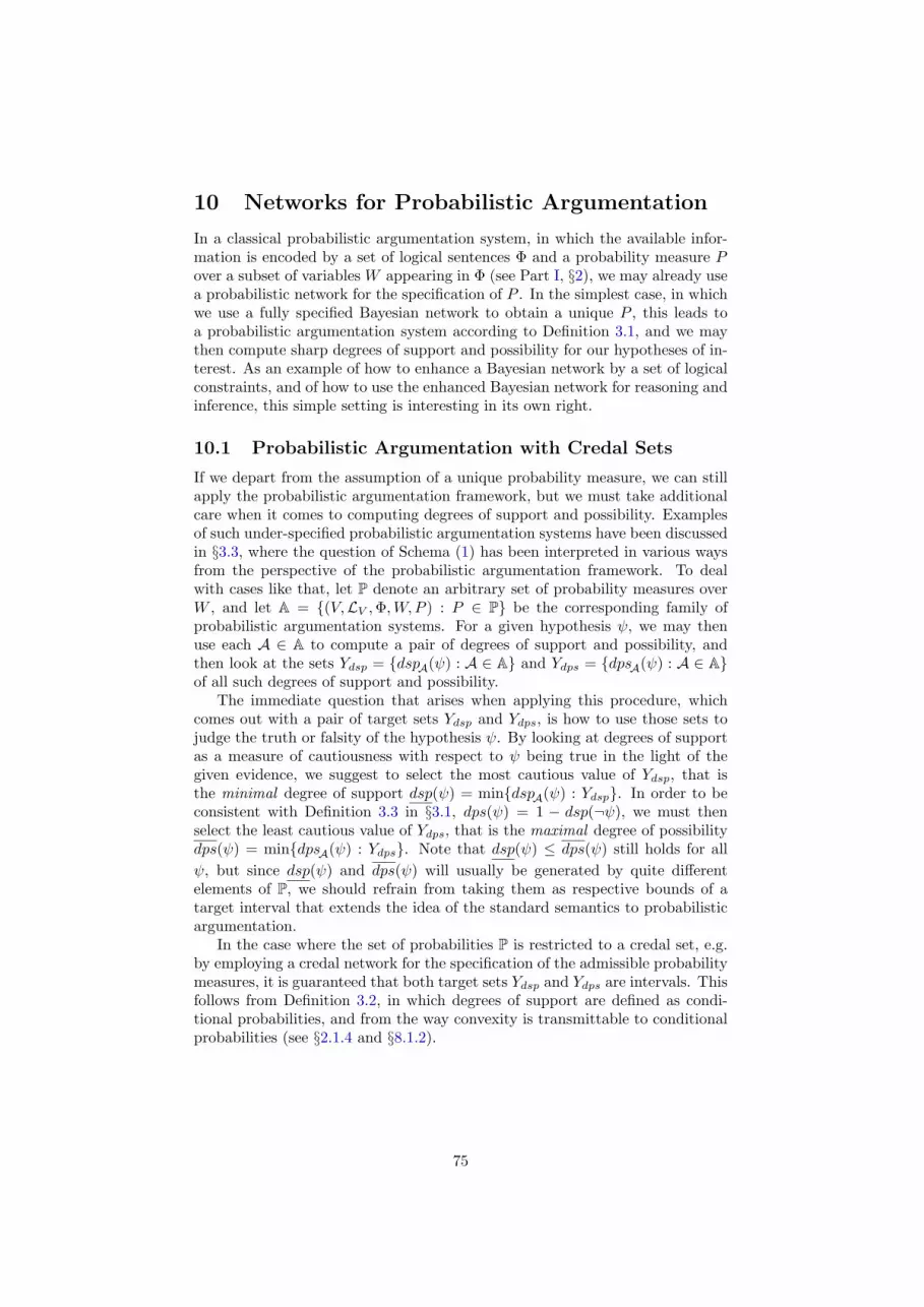
10 Networks for Probabilistic Argumentation

In a classical probabilistic argumentation system, in which the available infor-mation is encoded by a set of logical sentences Φ and a probability measure Pover a subset of variables W appearing in Φ (see Part I, §2), we may already usea probabilistic network for the specification of P . In the simplest case, in whichwe use a fully specified Bayesian network to obtain a unique P , this leads toa probabilistic argumentation system according to Definition 3.1, and we maythen compute sharp degrees of support and possibility for our hypotheses of in-terest. As an example of how to enhance a Bayesian network by a set of logicalconstraints, and of how to use the enhanced Bayesian network for reasoning andinference, this simple setting is interesting in its own right.

10.1 Probabilistic Argumentation with Credal Sets

If we depart from the assumption of a unique probability measure, we can stillapply the probabilistic argumentation framework, but we must take additionalcare when it comes to computing degrees of support and possibility. Examplesof such under-specified probabilistic argumentation systems have been discussedin §3.3, where the question of Schema (1) has been interpreted in various waysfrom the perspective of the probabilistic argumentation framework. To dealwith cases like that, let P denote an arbitrary set of probability measures overW , and let A = (V,LV ,Φ,W, P ) : P ∈ P be the corresponding family ofprobabilistic argumentation systems. For a given hypothesis ψ, we may thenuse each A ∈ A to compute a pair of degrees of support and possibility, andthen look at the sets Ydsp = dspA(ψ) : A ∈ A and Ydps = dpsA(ψ) : A ∈ Aof all such degrees of support and possibility.

The immediate question that arises when applying this procedure, whichcomes out with a pair of target sets Ydsp and Ydps, is how to use those sets tojudge the truth or falsity of the hypothesis ψ. By looking at degrees of supportas a measure of cautiousness with respect to ψ being true in the light of thegiven evidence, we suggest to select the most cautious value of Ydsp, that isthe minimal degree of support dsp(ψ) = mindspA(ψ) : Ydsp. In order to beconsistent with Definition 3.3 in §3.1, dps(ψ) = 1 − dsp(¬ψ), we must thenselect the least cautious value of Ydps, that is the maximal degree of possibilitydps(ψ) = mindpsA(ψ) : Ydps. Note that dsp(ψ) ≤ dps(ψ) still holds for allψ, but since dsp(ψ) and dps(ψ) will usually be generated by quite differentelements of P, we should refrain from taking them as respective bounds of atarget interval that extends the idea of the standard semantics to probabilisticargumentation.

In the case where the set of probabilities P is restricted to a credal set, e.g.by employing a credal network for the specification of the admissible probabilitymeasures, it is guaranteed that both target sets Ydsp and Ydps are intervals. Thisfollows from Definition 3.2, in which degrees of support are defined as condi-tional probabilities, and from the way convexity is transmittable to conditionalprobabilities (see §2.1.4 and §8.1.2).

75

10.2 Constructing and Applying the Credal Network

In §3 we discussed two different types of semantics for Schema (1). The seman-tics of the first type in §3.3.1 are all extensions of the standard semantics tothe probabilistic argumentation framework, and we may thus follow a strategysimilar to the one outlined in §9 to construct a network. But this is not thecase for the semantics of the second type in §3.3.2, where each given probabilityset Xi is interpreted as a probability constraint for the reliability of a sourceproviding the premise ϕi. Moreover, by assuming the sources to be pairwiseindependent, it seems that the second type of semantics does not provide ad-equate grounds for constructing non-trivial networks. The discussion in theremaining of this section will therefore not further pursue this particular way ofinterpreting instances of Schema (1).

In the extended standard semantics of §3.3.1, we assume a set Φ of logicalconstraints to be given in addition to the premises on the left hand side ofSchema (1). For the premises to be useful to construct a network, let theminclude a set I of explicit probabilistic independencies, similar to §9.2. Notethat such independencies may be available e.g. from representing a probabilisticargumentation system in form of Schema (1) as proposed in §3.2. In general,the best we can do then is to apply Algorithm 9.1 to the set of premises to geta credal network that represents the corresponding credal set w.r.t. ΩW , whereW denotes the set of variables appearing in the premises.

This credal network together with the common machinery from §8.2 canthen be used to compute respective sets Ydsp and Ydps of degrees of support andpossibility for a given hypothesis ψ. For this, the following algorithm consist of3 steps: the first step is the network construction according to Algorithm 9.1,the second step is the determination of the sets ArgsA(ψ), ArgsA(¬ψ), andArgsA(⊥), and the third step is the application of the common machinery from§8.2 to approximate the target intervals. Note that by explicitly calling thecommon machinery in last step, this algorithm differs from the algorithms ofthe following sections. The reason for this is that we need to adapt the hill-climbing algorithm to approximate degrees of support and possibility instead ofprobabilities of normal events.

Algorithm 10.1 Construction and evaluation of a credal network for the ex-tended standard semantics, based on explicit independence assumptions and anadditional set of logical constraints.

Input: two sets W = A1, . . . , AM and V ⊇ W of propositional variables,a set I of probabilistic independence relations (of the form Ai ⊥⊥ Aj orAi ⊥⊥ Aj |Ak) and premises ϕX1

1 , . . . , ϕXNN involving variables from W , aset Φ of logical constraints involving variables from V , and a query ψ.

1. Network construction: Use Algorithm 9.1 to construct a credal networkthat represents I and ϕX1

1 , . . . , ϕXNN .

2. Computing arguments, counter-arguments, and conflicts: Usestandard inference techniques to compute logical representations α+, α−

and α⊥ of the sets ArgsA(ψ), ArgsA(¬ψ), and ArgsA(⊥), respectively,where A = (V,LV ,Φ,W, P ) is the involved probabilistic argumentationsystem (for some under-determined probability measure P ).

76

3. Target interval approximation:

(a) Transform α+, α−, and α− into disjoint sums-of-products (see §8.2.1).

(b) Compile the credal network (see §8.2.2) and instantiate it for each ofthe disjoint terms of α+, α−, and α⊥.

(c) Adapt and apply the hill-climbing algorithm from §8.2.3 to the com-piled network to approximate lower and upper bounds of

dsp(ψ) =P (α+)− P (α⊥)

1− P (α⊥)and dps(ψ) =

1− P (α−)1− P (α⊥)

.

Output: Inner approximations of the target intervals Ydsp and Ydps for the firstsemantics of §3.3.1.

Note that one of the computationally hardest tasks of the above algorithm isthe computation of the logical representations α+, α−, and α⊥ in the secondstep (their size is exponential in the worst case). Another difficult task is thetransformation of α+, α−, and α⊥ into disjoint sums-of-products (there are ex-ponentially many such terms in the worst case). We may thus need appropriateapproximation algorithms, for example one that computes the shortest termsfirst [47, 48]. By doing so, we may still get good approximations of the targetintervals, but we must be aware that they may no longer be inner approxima-tions.

With the above computational scheme, we obtain a way of extending thestandard semantics to the probabilistic argumentation framework, but not forthe further options given in §3.3.1. To extend it, for example for the semanticsthat takes each premise ϕXii as a constraint dsp(ϕ) ∈ Xi on respective degrees ofsupport, we must first compute respective logical representations αi for each setArgsA(ϕi) and for ArgsA(⊥), and then construct the credal network with respectto the constraints [P (α+) − P (α⊥)]/[1 − P (α⊥)] ∈ Xi. To get rid of the non-linearity of those expressions, we may consider k = 1− P (α⊥) to be a constantvalue and then consider respective linear constraints P (α+) − P (α⊥) ∈ kXi.This works in a similar way for constraints on degrees of possibility and forcombined constraints (see §3.3.1).

11 Networks for Evidential Probability

In §4 we discussed two different semantics for Schema (1) to answer two differenttypes of inferential question for the theory of evidential probability. The firstinterpretation given to Schema (1) is just the usual semantics of evidentialprobability, which we call first-order EP (§4.3.1). The second interpretationgiven to Schema (1) is a proposal to evaluate the robustness of a particularfirst-order EP assignment, which we call second-order EP (§4.3.3).

Each semantics leads to very different properties of the entailment relationin Schema (1), however. First-order EP is a non-probabilistic, sub-System Pnon-monotonic logic of probabilities, whereas second-order EP is a monotoneprobabilistic logic. Thus the inferential methods for each semantics is quitedifferent.

In this section we investigate how credal networks can be used to calculatean answer for second-order EP inference only, since first-order EP is essentially

77

a logic of probability statements rather than a probabilistic logic. Nevertheless,second-order EP depends crucially upon outputs from first-order EP-argumentsrepresenting all possible counter-factual EP arguments with respect to the ac-tually accepted evidence. So, we first present an algorithm for first-order EP,which does not rely upon credal networks, and then present an algorithm forconstructing a credal network that may exploit the common machinery of §8.2.

11.1 First-Order Evidential Probability

Algorithm 11.1 Computing First-order Evidential Probability.

Input: a pair 〈χ,Γδ〉, where χ is a formula and Γδ = ϕ1, . . . , ϕn a set offormulas of Lep.

1. Selection of potential probability statements: Given 〈χ,Γδ〉, con-struct the set Γ[χ] by Definition 4.2:

(a) Let Γ[χ] be the equivalence class defined by

%~x(τ(~x), ρ(~x), [l, u]) : χ ≡ τ(ω) ∧%(τ(ω), ρ(ω), [l, u]),

where each %~x(τ(~x), ρ(~x), [l, u]) of X is a direct inference statementof Γδ such that ~x is substituted by constants ω in τ and τ(ω) iscoextensive with χ.27

(b) The direct inference statements in Γ[χ] ⊆ Γδ are the potential prob-ability statements for χ.

2. Selection of relevant statistical statements: Given Γ[χ], constructthe set ΓRS[χ] ⊆ Γ[χ] by applying Richness and Specificity (§4.1.1):

(a) Define ΓR[χ] ⊆ Γ[χ] such that ∀ϕ, ϑ ∈ Γ[χ], if ϕ and ϑ conflict and ϕ isa marginal distribution and ϑ a joint-distribution, then ϑ ∈ ΓR[χ] butϕ 6∈ ΓR[χ].

i. Determining conflict: To determine whether direct inferencestatements ϕ, ϑ conflict, compare the interval [l, u] of ϕ to theinterval [k, t] of ϑ. Only 3 comparisons are necessary. Given[l, u]: accept that [k, t] conflicts with [l, u] if:· k < l and t < u, or· l > k and t > u, or· l = k and t = u.

ii. Distinguishing between a marginal distribution and ajoint-distribution: There is a syntactic difference between amarginal distribution whose statistic is n dimensions and a joint-distribution whose statistic is n+m dimensions, for some positivem. This will be expressed by the arity of the target formulapredicates (τ) appearing in ϕ and ϑ.

27Note that the sequence of constants ω must be such that the variable substitution of τ(ω)leaves no free variables in τ , but that ρ(ω) may have open variables. This will be importantin the implementation of the Richness rule. Also, we relax notation here by omitting thecorner-quotes.

78

(b) Define ΓRS[χ] ⊆ ΓR[χ] such that ∀ϕ, ϑ ∈ ΓR[χ], if ϕ and ϑ conflict but ρof ϕ and ρ′ of ϑ are such that ρ ⊂ ρ′, then ϕ ∈ ΓRS[χ] but ϑ 6∈ ΓRS[χ] .

i. Apply step 2.a.i. to determine conflict, replacing Γ[χ] with ΓR[χ].ii. Selecting specific statistics for χ: Specificity concerns ex-

plicit logical relationships between reference classes ρ of ϕ andρ′ of ϑ that appear in Γδ. Specificity applies to ϕ and ϑ whenboth are in ΓR[χ], the interval of ϕ conflicts with the interval of ϑbut ρ ⊂ ρ′.

3. Find the shortest cover: Given |ΓRS[χ] | = n, define Y = X1, . . . , Xn asthe set of n intervals expressed by the formulas in ΓRS[χ] . Apply Strength(§4.1.1) to Y closed under difference:

(a) If |ΓRS[χ] | = 0, return [0, 1].

(b) Sort Y = X1, . . . , Xn by the lower endpoints l11 , . . . , lnj in ascend-ing order. Name that sequence Y∗.

(c) Sort Y by the upper endpoints u11 , . . . , unj in descending order.Name that sequence Y∗. Then for j = 1 to n:

i. If |Y| = 1 and Y = [l, u], return [l, u].ii. If the max endpoint of ui of interval Xi of Y that is in the jth

position in Y∗ (ui ∈ Xi,j of Y∗) is not equal to the max endpointuk ∈ Xk,j of Y∗, then return [l, u′]; otherwise:

iii. If the max endpoint of ui ∈ Xi,j of Y∗ is equal to the maxendpoint uk ∈ Xk,j of Y∗, then eliminate Xi from Y∗ and fromY∗ and go to 3.c.i.

Output: An interval [l, u] corresponding to the proportion of EP models ofϕ1

1, . . . , ϕ1n that are also models of χ.

11.2 Second-Order Evidential Probability

The first-order question concerns the assignment of evidential probability to astatement given some evidence, which is captured in Schema (1) by the EPsemantics for |m. The second-order question concerns the proportion of overlapamong all possible combinations of evidence for ψ occurring in Γδ.

The second-order EP probability of ψ on evidence ϕX11 , . . . , ϕXnn is

P (ψ) =1∑

e1,...,em=0

P (ψ|ϕe11 , . . . , ϕemm ) · P (ϕe11 , . . . ϕ

emm ),

i.e., summing over all possible evidence for ψ with respect to Γδ, where P (ϕi) ∈[1− δ, 1] is the prior confidence in the evidence for ψ. In this paper we replaceP (ϕe11 , . . . ϕ

emm ) by

m∏

1

P (ϕeii ),

where P (ϕi) ∈ [λ, 1], λ = 1−δ. However, details about the theory of acceptanceare relevant in selecting λ. If we treat the interval [1 − δ, 1] as characterizing

79

the risk of accepting the set of premises, assign equal probability of risk of errorto each premise while assuming these probabilities are independent, then λ =1−δ 1

m . But the risk term δ typically is thought to characterize the inference foraccepting each statement, which is what motivates the approach adopted here.Furthermore, independence in second-order EP just says that the assignment offirst-order evidential probability to a conclusion depends only on the m piecesof possible evidence in Γδ for that conclusion, and the individual risk associatedwith accepting a false premise as a true one. A graphical representation of thedependency relations in a second-order EP inference is represented by the edgesin Figure 12.

!1 !2 !m

!

. . .

Figure 12: Second-order EP credal network.

We now present an algorithm for calculating second-order EP.

Algorithm 11.2 Computing Second-order Evidential Probability.

Input: ϕ[X1]1 , . . . , ϕ

[Xn]n |= ψ?, where ψ is the first-order EP assignment 〈χ, [l, u]〉

on the premises ϕ1, . . . , ϕn output by Algorithm 11.1.

1. Construction of graph:

(a) For Prob(χ,Γδ), construct the set ϕ1, . . . , ϕm = ∆ ⊆ Γδ of possibleevidence for χ with respect to Γδ (§4.3.2).

(b) Define the set of nodes V to include ϕ1, . . . , ϕm, ψ.(c) Connect arrows from each ϕi to ψ. (See Figure 12).

2. Probabilities:

(a) Attach: X1 to ϕ1, . . . , Xm to ϕm.

(b) Compute conditional probabilities: P (χ|ϕe11 , . . . , ϕemm ) = |[l,u]∩[l′,u′]|

|[l,u]| ,when ei = 1 ∨ ei = 0, for all 1 ≤ i ≤ m.

Output: a credal network with graph G, representing probabilistic indepen-dence relations implicit in second-order EP inference, and probabilitiescalculated as described above.

To compute Y for ψ, use the common machinery of §8.2.

12 Networks for Statistical Inference

In §5 we discussed two ways in which classical statistics can be captured inSchema (1), one using functional models and fiducial probability, and one usingevidential probability to represent the fiducial argument. This section investi-gates the use of the common machinery of §8.2 and Algorithm 11.1 in classicalstatistics.

80

H! D !

Figure 13: A network representing the conditional independencies between Hθ, ω andD in the functional model f(Hθ, ω) = D that generates the fiducial probability for Hθfrom the distribution over the stochastic elements ω.

12.1 Functional Models and Networks

As described in §5.1.2, one way of capturing classical statistics in Schema (1)makes use of fiducial probability and functional models: on the basis of aninvertible functional relation f(Hθ, ω) = d between data D, stochastic elementsω, and hypotheses Hθ, a probability assignment P (ω) determines a probabilityassignment P (Hθ). While the use of fiducial probability in Schema (1) is ratherlimited, we want to present a way in which credal networks may be used to aidthe computation of fiducial probability.

12.1.1 Capturing the Fiducial Argument in a Network

To set the stage, we first provide a network representation for the fiducial infer-ence represented by functional models. We restrict attention to fiducial proba-bility using an invertible functional relation. It may be recalled from §5.1.2 thatwe can relax the requirement of invertibility for the functional relation f , andderive degrees of support and possibility for a hypothesis HI consisting of a setof hypotheses Hθ. However, we will not discuss the generalisation to degrees ofsupport and possibility here.

In a fiducial argument, the relation between the hypotheses Hθ, the stochas-tic elements ω, and the data D is such that the stochastic elements and thehypotheses are probabilistically independent:

P (Hθ, ω) = P (Hθ)P (ω). (28)

Moreover, given a hypothesis hθ and a stochastic element ω, the occurrence ofthe data d is completely determined, P (d|hθ, ω) = Id(hθ, ω) where Id(hθ, ω) = 1if f(hθ, ω) = d and Id(hθ, ω) = 0 otherwise. The corresponding network isdepicted in Figure 13.

If we condition on the observed data d then, because of the network structureand the further fact that the relation f(Hθ, ω) is deterministic, the variablesω and Hθ become perfectly correlated: each hθ is associated with some ω =f−1(hθ, d). Assuming that the observation of d does not itself influence theprobability of ω, meaning that P (ω|d) = P (ω) we can therefore write

P (Hθ|d) = P (f−1(Hθ, d)) = P (ω). (29)

This means that after observing d we can transfer the probability distributionover ω to Hθ according to the function f−1.

12.1.2 Aiding Fiducial Inference with Networks

We now turn to the use of networks in aiding fiducial inference. The naturalsuggestion is to consider cases in which there are many different statistical pa-rameters θj in the model, and equally many observed variables Dj that may be

81

used to perform fiducial arguments. We may then employ independence rela-tions that obtain between the parameters and the data to speed up the fiducialinference.

Example 12.1 Consider hypotheses Hθ determined by two variables, θ = 〈θ1, θ2〉,stochastic elements ω = 〈ω1, ω2〉, and two propositions D1 and D2 representingthe data. Say that we have a number of independence relations between thesevariables and data sets:

P (D1 ∧D2|Hθ ∧ ω) = P (D1|Hθ1 ∧ ω1)P (D2|Hθ1 ∧Hθ2 ∧ ω2), (30)P (Hθ) = P (Hθ1)P (Hθ2), (31)P (ω) = P (ω1)P (ω2). (32)

Finally, we have smoothly invertible functional relations f(Hθ1 , ω1) = D1 andfθ1(Hθ2 , ω2) = D2, meaning that for each fixed value of θ1 the function fθ1 issmoothly invertible. The corresponding network is depicted in Figure 14.

D1

D2

!1

!2

H!1

H!2

Figure 14: A network representing the conditional independencies between Hθ, ω andD as expressed in Equations (30) to (32).

We first derive a fiducial probability P (Hθ1 |d1), whereby we assume that we donot yet have knowledge of D2 or Hθ2 . After that we derive a fiducial probabilityfor Hθ2 from d2, by first computing a fiducial probability over Hθ2 for each valueof θ1 separately. We then use the law of total probability to arrive at P (Hθ2 |d2).

This is a version of the so-called step-by-step method for the fiducial argument.See Seidenfeld [127]. The method was devised by Fisher for deriving the fiducialprobability over statistical hypotheses characterised by more than one parame-ter. We can easily generalise the application of networks to step-by-step fiducialinference for larger numbers of statistical parameters, data sets, and stochasticelements.

Algorithm 12.2 Construction of a network for fiducial inference over morethan one statistical parameter.

Input: The following assumptions to run the step-by-step fiducial argument.

1. A sample space ΩD involving propositional variablesD = D1, . . . DN,a model ΩH of hypotheses Hθ with θ = 〈θ1, . . . , θN 〉, and a space ofstochastic elements ΩW = 〈ω1, . . . ωN 〉.

2. Smoothly invertible functional relations fSjj (Hθj , ωj) = Dj in whichSj ⊆ θj′ : j′ < j, such that step-by-step fiducial inference can besupported. The sets Sj determine which hypotheses need to be fixedfor the functional relations fSjj to be smoothly invertible.

82

3. A set of independence relations I among the marginal probabilitiesP (Hθj ) of the hypotheses. Next to P (D1|Hθ) = P (D1|Hθ1), this setmust include the following independence relations for each j > 1:

P (Dj ∧Dj−1|Hθ) = P

Dj−1|

∧

j′∈Sj−1

Hθj′

P

Dj |

∧

j′∈SjHθj′

,

P (Hθ) =∏

j

P (Hθj ),

P (ω) =∏

j

P (ωj),

Construction of the network: run Algorithm 9.1 with the indepen-dence relations I to arrive at a network for fiducial inference.

Output: a network structure in which fiducial inference can be performed.

It must be conceded that the algorithm for setting up a network for fiducialinference requires a lot of input. This is because the fiducial argument itself canonly be run under fairly specific circumstances. Still, once the network is built,it will structure and possibly simplify the calculation of fiducial probability. Theidea is again that once the network has been built, computation is much lesscostly.

12.1.3 Trouble with step-by-step fiducial probability

As already indicated at the start of this section, fiducial probabilities are con-troversial, and this is all the more so for the step-by-step procedure. We explainbriefly why we recommend caution in the application of the step-by-step fiducialargument.

Returning to the example, note that we can only apply the fiducial argumenton the condition that, in the absence of knowledge about Hθ2 , the data D1 in-deed allow for transferring the probability assignment over ω1 to the hypothesesHθ1 . Now it seems that this possibility is guaranteed by the use of the smoothlyinvertible functional relation f(Hθ1 , ω1) = D1. But there is something a bitawkward about the assumption of the absence of knowledge about Hθ2 and theuse of the function f , which is brought out in Seidenfeld [126].

Imagine that we do have some fixed probability assignment P (Hθ2) beforewe apply the fiducial argument to derive P (Hθ1) from d1. Now consider thegraph in Figure 14. From this graph we can deduce that if there is some defi-nite probability assignment P (Hθ2), learning about D2 will be probabilisticallyrelevant to the probability of Hθ1 . Of course, there are special cases of prob-ability assignments P (Hθ1) for which the data on D2 come out as irrelevantanyway, but this is not the case in general. Hence, by the assumption of a par-ticular distribution P (Hθ1) we might destroy the smoothly invertible relationf(Hθ1 , ω1) = D1 and replace it with f(Hθ1 , ω) = D, in which case the fiducialargument cannot be run.

This makes step-by-step fiducial inference more problematic than its simpleand direct application. Moreover, there is no suggestion that network structurescan help to clear up the problem. The network of §12.1.1 provides a particular

83

perspective on the fiducial argument, but this perspective is not particularlyhelpful in framing the difficulties associated with the step-by-step procedure.Whether a more elaborate representation of the functional relations in terms ofnetworks would do better on this count is a question for further research.

12.2 Evidential Probability and the Fiducial Argument

The novelty of the fiducial argument is to treat indirect inference as a formof direct inference, and the approach that EP takes is to use knowledge aboutthe sample and the sampling procedure to eliminate those reference statisticsfrom which we have reason to believe are not representative. Since there isno network structure for first-order EP, the role that absence of knowledgeplays in the fiducial argument is viewed not as an awkward feature of Fisher’sargument but rather a central feature of statistical inference as such. We notedin §5.1.3 the clash between EP’s logic of probabilities and probabilistic logic,and with it the prospects of viewing classical statistical inference in terms of aprobabilistic logic. But the view does give a picture of statistical inference as aform of uncertain inference, and we may use the machinery developed in §11 tocalculate fiducial probabilities.

12.2.1 First-order EP and the Fiducial Argument

To interpretϕX1

1 , . . . , ϕXnn |≈ ψ?,

as an EP reconstruction of fiducial inference, we replace |≈ by |m of first-orderEP-entailment and interpret the premises to include logical information anddirect inference statements, just as we do §11, and add a selection functionf(χ,U(x)[x/ω]) ≥ λ that restricts the set of relevant direct inference statementsto just those that are rationally representative of χ to at least degree λ.

As we observed in §11, first-order EP does not admit the use of the commonmachinery of §8.2. We instead have Algorithm 11.1 to calculate first-order EPassignments. Thus there is no inferential machinery called upon apart fromwhat is provided by first-order EP.

As we observed in §5.3, this approach does not resolve the controversy sur-rounding the fiducial argument but instead pinpoints the where the controversylies, which is how to restrict (or, rather, rule out) otherwise applicable refer-ence statistics. Viewed in terms of a first-order EP inference, this restrictionwill involve logical formulas in our knowledge base that fix a subset of relevantstatistics to accept as rationally representative for a particular assignment [l, u]to χ.

12.2.2 Second-order EP and the Fiducial Argument

The first-order question concerns the assignment of evidential probability toa statement under the restriction of the pair (f, λ), where f is the ‘rationally-representative to degree λ’ selection function f(χ,U(x)[x/ω]) ≥ λ on the relevantstatistics for a sentence χ. The second-order question concerns the proportionof overlap among all possible combinations of evidence for ψ occurring in Γδunder the restriction (f, λ).

84

The second-order EP probability of ψ restricted by (f, λ) on the knowledgebase Γδ = ϕX1

1 , . . . , ϕXnn is

P (ψ) =1∑

e1,...,em=0

P (ψ|ϕe11 , . . . , ϕemm ) · P (ϕe11 , . . . ϕ

emm ),

where∑1e1,...,em=0 P (ψ|ϕe11 , . . . , ϕ

emm ) sums over all possible evidence given the

restriction imposed by (f, λ) for ψ with respect to Γδ. We replace P (ϕe11 , . . . ϕemm )

bym∏

1

P (ϕeii ),

where P (ϕi) ∈ [λ, 1], λ = 1− δ.Once (f, λ) picks ϕX1

1 , . . . , ϕXmm from ϕX11 , . . . , ϕXnn , the algorithm for

calculating the second-order EP probability for a fiducial argument is just thealgorithm for second-order EP, Algorithm 11.2.

13 Networks for Bayesian Statistical Inference

The essential property of Bayesian statistical inference, as introduced in §6, isthat the probability space includes both the sample space ΩD, consisting ofpropositional variables Di, and the space of hypotheses ΩH . In the semanticsof Bayesian statistical inference, the premises include a prior over hypothesesP (Hj) and the likelihoods of the hypotheses P (Di|Hj). The conclusion is aposterior over hypotheses P (Hj |des) for some observed assignment des to the Di,where e is a vector of assignments and s is a corresponding vector of values fori. In the following we will present two ways in which credal networks may beemployed in this inference. The first presents a computational improvement ofthe inferences as such, while the second supplements the inference with furthertools, deriving from the common machinery of §8.

13.1 Credal Networks as Statistical Hypotheses

We first spell out how a credal network can be related to a statistical model, i.e.a set of statistical hypotheses. Recall that a credal network is associated with acredal set, a set of probability functions over some designated set of variables.Hence a credal set may be viewed as a statistical model: each element of thecredal set is a probability function over the set of variables, and this probabilitymay be read as a likelihood of some hypothesis for observations of valuationsof the network. Conversely, any statistical model concerns inter-related trialsof some specific set of variables, so that we can identify any statistical modelwith a credal network containing these variables. Here we deal with non-causalstatistical hypotheses; [96, Chapter 4] argues that credal nets can also be usedto represent causal hypotheses.

13.1.1 Construction of the Credal Network

To construct the credal network that represents a statistical model, we first listall the independence relations that obtain between the variables in the samplespace ΩD.

85

Example 13.1 Consider subsequent observations, at times i, of three binaryvariables Vi = Ai, Bi, Ci. The independence relations I are as follows:

∀i :Ai ⊥⊥ Bi|Ci−1,

∀i′ 6= i− 1 :Ai ⊥⊥ Ci′ , Bi ⊥⊥ Ci′ ,∀i′ 6= i : Ci ⊥⊥ Ci′ , Ai ⊥⊥ Ai′ , Bi ⊥⊥ Bi′ , Ai ⊥⊥ Bi′ , Bi ⊥⊥ Bi′ .

To determine the credal network, we run the algorithm of section §9.2, whichalso allows us to include further constraints ϕXii on the probability assignmentsof the variables.

Algorithm 13.2 Construction of a credal network for the semantics of Bayesianstatistical inference, based on a given model of statistical hypotheses.

Input: a model ΩH of statistical hypotheses Hθ, a sample space ΩD concerninga set V = A1, . . . , AM of propositional variables, and further premisesϕX1

1 , . . . , ϕXNN involving those variables.

1. Derivation of the independence relations: using the (conditional)independence relations inherent to the likelihoods of all the Hθ

(a) If P (Ai ∧Aj | Hθ) = P (Ai | Hθ)P (Aj | Hθ), add Ai ⊥⊥ Aj to the setof independence constraints I.

(b) If P (Ai∧Aj |∧k Ak∧Hθ) = P (Aj |

∧k Ak∧Hθ)P (Aj |

∧k Ak∧Hθ),

add Ai ⊥⊥ Aj |∧k Ak to the set of independence constraints I.

2. Running Algorithm 9.1: based on the set I of independence relationsand the premises ϕX1

1 , . . . , ϕXNN .

Output: a graph G and a set of extremal points vi in terms of the networkcoordinates.

As the corresponding credal set we take the complete extension of the network.Under this extension, the credal set is basically a set of Bayesian networks thatall have the given credal network as their graph. The fact that the statisticalmodel is thus associated with a Bayesian network containing free coordinateswill turn out to be useful in learning from data.

Now that we have identified credal sets as statistical models, the notion of asecond-order probability assignment falls into place quite naturally. The second-order probability assignment takes the members of the credal set as arguments.Any credal set may be captured by a second-order probability over probabilityfunctions of the variables that is non-zero only at those functions belonging tothe credal set. A uniform distribution is perhaps the most natural choice, butother shapes of the second-order probability are possible too.

Example 13.3 (continued) Recall example Example 13.1. Even if we restrictattention to Markov processes with these variables, a statistical hypothesis onthem is determined by 23(23 − 1) = 56 probabilities for the transitions betweenvaluations of the variables. So the corresponding statistical model Θ has a coor-dinate system with 56 coordinates. Now consider the network that captures theindependence relations.

86

Ai BiCi!1

Figure 15: The graph capturing the independence relations among the propositionalvariables Ai, Bi, and Ci. This graph holds for each and every value of i.

The complete extension of this network consists of the probability functions ar-rived at by filling in the probabilities on the nodes and edges. Again each of thesefunctions is associated with a statistical hypothesis, denoted Hη. The coordinatesystem of the corresponding model Θnet is a vector η = 〈γ, α0, β0, α1, β1〉, where

P (ci|Hη) = γ,

P (ai+1|cki ∧Hη) = αk,

P (bi+1|cki ∧Hη) = βk.

The space Θnet is a strict subset of the space Θ. The above credal network maybe characterised by a prior probability assignment that is nonzero only on thissubset.

Against the background of a statistical model as the complete extension ofa credal network, we first discuss Bayesian statistical inference as it has beenpresented in the foregoing. For a more complete example of the applicationof credal networks in the context of Bayesian inference over both latent andobservable variables, see [122]. Section §13.2 concerns an extension of Bayesianstatistical inferences on this basis.

13.1.2 Computational Advantages of Using the Credal Network

We consider inferences to do with adapting the second-order probability assign-ment over the credal set according to Bayesian statistical inference, on the basisof repeated observations of the variables.

One important consequence of viewing the statistical model as a credal net-work is that it allows us to reduce the dimensions of the statistical model, as theabove example illustrates: the credal network restricts the space of allowed pa-rameter values from dim(Θ) = 56 to dim(Θnet) = 5 dimensions. This reductionin the dimensions of the model can entail major reductions in computationalload, parallel to the reduction in computational load effected by using Bayesiannetworks when dealing with single probability assignments.

Another important consequence concerns the coordinate system of the sta-tistical model. Note that by replacing the product of simplexes Θ with thespace Θnet, we are not only reducing the number of coordinates, but we are alsoavailing ourselves of coordinates that are orthogonal to each other. If we wantto update the probability assignment over the model with the observation of onevariable, while the observations of other variables are unknown, this can moreeasily be captured analytically in the coordinate system deriving from the credalnetwork. In particular, if we start out with a prior probability density over themodel that is factorisable, P (Hη) = fC(γ)fA0(α0)fB0(β0)fA1(α1)fB1(β1), up-dates on the variables run entirely separately. So if we find the assignment ciafter some sequence of particular observations d, we need only adapt the densityfactor fC(γ|d) to fC(γ|d∧ci). The other factors are invariant under this update.

87

This computational advantage shows up in the predictive probabilities thatderive from the posterior probability assignments over the model. As indicatedin §6, if the probability density over statistical hypotheses is a Dirichlet dis-tribution, then the predictions for valuations of the separate network variablesare Carnapian prediction rules. Consequently, entire network valuations arepredicted according to products of such prediction rules, as is worked out inmore detail in Romeijn [121]. There it is also explained that the use of thecoordinate system deriving from the network helps us to define and motivatealternative prior probability assignments over the model, allowing us to capturevariations in inductive influences among valuations of the network. In Romeijn[120] these insights are generalised to prior probability densities outside thefamily of Dirichlet priors.

In sum, credal networks can be used to improve computation in Bayesianstatistical inferences. However, there is not a direct application of the commoninference machinery of §8 to this use of credal networks. Rather the present us-age remains internal to the inference machinery provided by Bayesian statisticsitself, which employs probability density functions over the credal set. In the re-mainder of this section we turn to an application of credal networks that directlyemploys the common inference machinery. This involves a genuine extension ofBayesian statistical inference itself.

13.2 Extending Statistical Inference with Credal Networks

In this section we include the statistical hypotheses in a credal network repre-sentation, and investigate some of the evidential and logical relations betweenhypotheses and observed variables.

13.2.1 Interval-Valued Likelihoods

In the foregoing we have associated statistical hypotheses with probability as-signments in the credal set: every hypothesis is associated with a single suchlikelihood function, and thus with a single probability assignment over the ob-servable variables. But we may also add the hypotheses as nodes in the network.

Example 13.4 Consider a credal network consisting of a hypothesis node Hj

with j ∈ 0, 1 and a large number of instantiation nodes of the propositionalvariables Ci, labelled with i.

Hj

C1 C2 Ci. . . . . .

Figure 16: A graph containing the statistical hypothesis Hj as the top node. Condi-tional on the hypothesis, the propositional variables Ci for i = 1, 2, . . . are independent.

These instantiation variables are independent of each other conditional on Hj,and each value j may be associated with a conditional probability of each of the

88

instantiations. These conditional probability assignments can be filled in on theedges leading from the hypothesis node Hj to the separate instantiations of Ci.

The idea to include a hypothesis in a credal network leads quite naturallyto the idea of interval-valued likelihoods. That is, we may assign a probabilityinterval to the edges connecting a statistical hypothesis with the data. Illus-trating this by the above example, we replace the sharp probability values forci with

P (ci|H0) ∈ [0.3, 0.7], (33)P (ci|H1) ∈ [0.6, 0.8]. (34)

In words, this expresses that the statistical hypotheses are not exactly clearon the probability of ct, although they do differ on it. The use of this formalpossibility is in a sense complementary to the well-known method of Jeffreyconditioning. Jeffrey conditioning tells us what to do in case we are not quitesure what the evidence we gathered is, while we are sure how the evidence, oncemade precise, bears on the hypotheses; this is expressed in the condition of rigid-ity. The interval-valued likelihoods, by contrast, provide us with a technique toupdate probability assignments in case we know exactly what evidence we havegathered, while we are not sure how this evidence bears on the hypotheses atissue.

The idea of interval-valued likelihoods is not new; it has already been dealtwith by Halpern and Pucella [59]. There the updates of probability assignmentsare carried out using Dempster’s rule of combination. The advantage of pre-senting the idea in the context of Schema (1) is that we can directly use thecommon inference machinery. Starting with an unknown probability for bothHj , for example P (Hj) ∈ [0, 1], we may input the instantiations of several ci, toarrive at new interval-valued probability assignments for both hypotheses. Thecommon machinery of credal networks, as worked out in §8, can thus be applieddirectly to the statistical setting.

Algorithm 13.5 Construction of a credal network for Bayesian statistical in-ference in which the statistical hypotheses are included.

Input: a finite set of credal sets Kj for j = 1, . . . N , each based on a given set ofpropositional variables V = A1, . . . AM, independence relations I, andpremises ϕXii , such that the sets are all associated with a unique credalnetwork G.

1. Addition of hypotheses nodes: add the node Hj with possible valua-tions j = 1, . . . N , and connect the node Hj with each variable Aj in thegraph G.

2. Fixing the likelihoods: associate each credal set Kj with a statisticalhypothesis Hj , by setting the credal set for the variables V to Kj for thevaluation j of the hypothesis node Hj .

Output: a statistical model in which each hypothesis Hj is associated with acredal set over the variables V .

89

We can then use the common machinery to calculate the interval-valued prob-abilities that attach to the respective statistical hypotheses Hj . We think thatthis can be useful to both statisticians and working scientists. It frequentlyhappens that the bearing of some piece of evidence on the available hypothesesis somehow vague.

13.2.2 Logically Complex Statements with Statistical Hypotheses

The idea to include hypotheses in the credal network invites a further applicationthat derives from the standard semantics.

Taken by themselves, second-order probabilities over statistical hypothesesallow one to infer various useful quantities, such as expectation values and pre-dictions. By including the statistical hypotheses in the credal network, we canalso infer probability assignments over logically complex propositions concern-ing statistical hypotheses, these inferred quantities, and the data. Importantly,it allows us to assess the logical combination of statistical hypotheses from anal-yses concerning overlapping sets of propositional variables.

As briefly discussed at the end of §6, we must be careful in interpreting theresulting probability assignments over logically complex propositions involvinghypotheses, which are typically interval-valued. The interval-valued assignmentsto such propositions cannot be interpreted as credence intervals: they pertain toa single statistical hypothesis and not to a range of values of statistical parame-ters. The shape of the second-order probability, as introduced in the precedingsection, tells us a lot more about the uncertainty over the probabilities assignedto variables, and such uncertainty over probabilities is simply not expressed inthe interval probabilities of credal networks.

Statisticians may nevertheless make good use of credal networks that includestatistical hypotheses. Often enough the proposition of interest in a scientificenquiry is logically complex, and very often the background knowledge containslogically complex propositions. With the above ideas in place, Schema (1) pro-vides a systematic way of dealing with such pieces of background knowledge.

14 Networks for Objective Bayesianism

According to the objective Bayesian semantics, ϕX11 , ϕX2

2 , . . . , ϕXnn |≈ ψY if andonly if all the probability functions that satisfy the constraints imposed by thepremisses and that are otherwise maximally equivocal, also satisfy the conclu-sion.

As outlined in §7, the left-hand side is interpreted as the set of directly trans-ferred constraints χ. One then determines the set P∗χ of probability functionsthat satisfy maximally consistent subsets of χ and takes the convex closure [P∗χ]of this set to yield the set E of probability functions compatible with the agent’sepistemic background E . Note that since X1, . . . , Xn are closed intervals, Pχ isalready closed and convex. Assuming that the premisses ϕX1

1 , ϕX22 , . . . , ϕXnn are

consistent, E = [P∗χ] = Pχ. Hence under the assumption of consistency we cansimply consider maximally equivocal probability functions from all those thatsatisfy the premisses.

90

14.1 Propositional Languages

Suppose further that ϕ1, . . . , ϕn, ψ are sentences of a finite propositional lan-guage L with propositional variables A1, . . . , An. Then entropy is a measureof the degree to which a probability function equivocates and there is a uniqueentropy maximiser. In principle then we consider only a single model of thepremises—the probability function that has maximum entropy from all thosethat satisfy the premises—and see whether that model satisfies the conclusion.This model can be represented by a Bayesian network, and one can use this net-work to calculate the probability Y to attach to the conclusion sentence ψ. ABayesian network that represents a probability function that represents degreesof belief that are deemed rational according to objective Bayesian epistemol-ogy is called an objective Bayesian network [150]. In our scenario an objectiveBayesian network can be constructed as follows.

Algorithm 14.1 Construction of an objective Bayesian network—a Bayesiannetwork for the objective Bayesian semantics—on a propositional language.

Input: ϕX11 , . . . , ϕXnn , ψ where ϕ1, . . . , ϕn, ψ are sentences of a finite proposi-

tional language.

1. Construction of the graph:

(a) Construct an undirected constraint graph G by taking the proposi-tional variables occurring in ϕ1, . . . , ϕn, ψ as nodes and connectingtwo variables with an edge if they occur in the same premise ϕi.

(b) Transform G into a DAG H:

i. Triangulate G to give GT .ii. Reorder the variables according to maximum cardinality search.iii. Let D1, . . . , Dl be the cliques of GT , ordered according to highest

labelled vertex.iv. Let Ej = Dj ∩ (

⋃j−1i=1 Di) and Fj = Dj\Ej , for j = 1, . . . , l.

v. Construct a directed acyclic graph H by taking propositionalvariables as nodes, and• Add an arrow from each vertex in Ej to each vertex in Fj ,

for j = 1, . . . , l.• Add further arrows, from lower numbered variables to higher

numbered variables, to ensure that there is an arrow betweeneach pair of vertices in Dj , j = 1, . . . , l,.

2. Derivation of the conditional probability functions: Find the valuesof P (aei | parei ) that maximise the total entropy

H = −n∑

i=1

∑

e∈0,1|Anc′i|

∏

Aj∈Anc′i

P (aej |parej)

logP (aei |parei ),

where Anc′i is the set consisting of Ai and its ancestors in H. (Herestandard numerical techniques or Lagrange multiplier methods can beused.)

91

A1 A2

A3

A4

A5

Figure 17: Constraint graph.

A1 A2

A3

A4

A5

Figure 18: Graph satisfying the Markov condition.

Output: H, P (aei | parei ) : i = 1, . . . , n, e ∈ 0, 1n

The output of this algorithm is provably a Bayesian network representation ofthe maximum entropy probability function P , from all those that satisfy theinput [149, §5.7]. This objective Bayesian network can be used to calculateY = P (ψ), as indicated in §8.

Example 14.2 Suppose we have a question of the form:

a1 ∧ ¬a2[0.8,0.9], (¬a4 ∨ a3)→ a2

0.2, a5 ∨ a3

[0.3,0.6], a40.7 |≈ a5 → a1

?

This is short for the following question: given that a1 ∧ ¬a2 has probabilitybetween 0.8 and 0.9 inclusive, (¬a4 ∨ a3) → a2 has probability 0.2, a5 ∨ a3 hasprobability in [0.3, 0.6] and a4 has probability 0.7, what probability should a5 → a1

have? As explained in §7.3, this question can be given an objective Bayesianinterpretation: supposing the agent’s evidence imposes the constraints P (a1 ∧¬a2) ∈ [0.8, 0.9], P ((¬a4∨a3)→ a2) = 0.2, and P (a5∨a3) ∈ [0.3, 0.6], P (a4) =0.7, how strongly should she believe a5 → a1? By means of Algorithm 14.1, anobjective Bayesian network can be constructed to answer this question. Firstconstruct undirected constraint graph, Figure 17, by linking variables that occurin the same constraint. Next, follow the algorithm to transform the undirectedgraph into a directed acyclic graph satisfying the Markov condition, such asFigure 18. The third step is to maximise entropy to determine the probabilitydistribution of each variable conditional on its parents in the directed graph. Thisyields the objective Bayesian network. Finally we use the network to calculatethe probability of the conclusion: here we apply the common machinery of §8.2.In fact in this simple example calculating the probability of the conclusion isvery straightforward:

P (a5 → a1) = P (¬a5 ∧ a1) + P (a5 ∧ a1) + P (¬a5 ∧ ¬a1)= P (a1) + P (¬a5|¬a1)(1− P (a1))

Thus we must calculate P (a1) and P (¬a5|¬a1) from the network.

92

14.2 Predicate Languages

If ϕ1, . . . , ϕn, ψ are sentences of a predicate language, a similar procedure canbe applied.

The simplest case is that in which the constraints imposed by the left-handside of the fundamental question, ϕX1

1 , ϕX22 , . . . , ϕXnn , constrain finitely many

atomic sentences (sentences of the form Ut). This occurs for example when thelanguage is finite (i.e., there are finitely many constant, predicate, relation andfunction symbols), or when the sentences ϕ1, . . . , ϕn, ψ are all quantifier-free.Let a1, a2, . . . , ak be the atomic sentences constrained by ϕX1

1 , ϕX22 , . . . , ϕXnn .

Then we construct the objective Bayesian network exactly as in Algorithm 14.1,taking variables corresponding to these atomic sentences as nodes in the graph.(As pointed out in §7, in this finite case minimising distance to the equivocatoris equivalent to maximising entropy.) The objective Bayesian network can thenbe used to calculate P (ψ) as discussed in §8.

In the more general situation—with an infinite predicate language and ar-bitrary sentential constraints—steps need to be taken to ensure the Bayesiannetwork remains finite (in order to use the network for computation). In thiscase we can use the following algorithm:

Algorithm 14.3 Construction of an objective Bayesian network on a predicatelanguage.

Input: ϕX11 , . . . , ϕXnn , ψ where ϕ1, . . . , ϕn, ψ are sentences of a predicate lan-

guage and ψ is quantifier-free.

1. Construction of the graph:

(a) Instantiate all quantified premise sentences as follows. Let t1, . . . , tmbe the constant symbols appearing in ϕ1, . . . , ϕn, ψ. For a sentence ϕlet |ϕ| be the number of distinct variables occurring in ϕ. For a tuplet of |ϕi| constants selected from t1, . . . , tm, let ϕi/t be the result ofsubstituting each distinct variable in ϕi for the corresponding con-stant in t. (If ϕi is quantifier-free, |ϕi| = 0, take ϕi/t to be ϕi.) Fori = 1, . . . , n let Φi be the set of all such instantiations, Φi = ϕi/t :some t.

(b) Construct an undirected constraint graph G:

i. Let a1, . . . , ak be the atomic sentences occurring in Φ1, . . . ,Φnand ψ. Construct binary variables A1, . . . , Ak such that each Aihas ai and ¬ai as possible assignments. Take these variables asthe nodes of G.

ii. Connect two variables Ai and Aj with an edge if ai and aj occurin sentences in the same Φk (i.e., if they occur in instances of thesame premise sentence ϕk).

(c) Transform G into a DAG H:

i. Triangulate G to give GT .ii. Reorder the variables according to maximum cardinality search.iii. Let D1, . . . , Dl be the cliques of GT , ordered according to highest

labelled vertex.iv. Let Ej = Dj ∩ (

⋃j−1i=1 Di) and Fj = Dj\Ej , for j = 1, . . . , l.

93

A1 A2 A3 A1 A2 A3

Figure 19: Constraint graph (left) and graph satisfying the Markov Condition (right).

v. Construct a directed acyclic graphH by taking variablesA1, . . . , AKas nodes, and• Add an arrow from each vertex in Ej to each vertex in Fj ,

for j = 1, . . . , l.• Add further arrows, from lower numbered variables to higher

numbered variables, to ensure that there is an arrow betweeneach pair of vertices in Dj , j = 1, . . . , l,.

2. Derivation of the conditional probability functions: Find the valuesof P (aei | parei ) induced by a function P on the predicate language thatsatisfies the input constraints and is closest to the equivocator.

Output: H, P (aei | parei ) : i = 1, . . . , n, e ∈ 0, 1n

That the graph represents the independencies of the function P that satisfies theconstraints and is closest to the equivocator follows for the same reasons as inthe case of Algorithm 14.1 [149, §5.7]. As in the case of Algorithm 14.1 we leavethe methods for filling in the conditional probability functions unspecified: whatis important for the purposes of this paper is the dimension reduction offeredby representing P by a Bayesian network factorisation of P with respect to H.

Here is a simple example.

Example 14.4 Suppose we have a question of the form:

∀x(Ux→ V x)3/5,∀x(V x→Wx)3/4

, Ut[0.8,1] |≈Wt?

By means of Algorithm 14.3, an objective Bayesian network can be constructedto answer this question. There is only one constant symbol so instantiating theconstraint sentences gives Φ1 = Ut → V t,Φ2 = V t → Wt,Φ3 = Ut.Let A1 take assignments Ut (assignment a1) and ¬Ut (assignment a1), A2 takeassignments Vt (a2) and ¬V t (a2) and A3 take assignments Wt (a3) and ¬Wt(a3). Then G and H are depicted in Figure 19. It is not hard to see thatP (a1) = 4/5, P (a2|a1) = 3/4, P (a2|¬a1) = 1/2, P (a3|a2) = 5/6, P (a3|¬a2) =1/2; together with H, these probabilities yield a Bayesian network. The commonmachinery of §8.2 then gives us P (a3) = P (Wt) = 11/15 as an answer to ourquestion.

15 Conclusion

In this paper we have argued in favour of two basic claims:

Part I: a unifying framework for probabilistic logic can be constructed aroundwhat we have called the Fundamental Question of Probabilistic Logic, orsimply Schema (1);

94

Part II: probabilistic networks can provide a calculus for probabilistic logic—in particular they can be used to provide answers to the fundamentalquestion.

These two claims constitute what we call the progicnet programme, and offera means of unifying various approaches to combining probability and logic in away that seems promising for practical applications.

Because of this twin focus and the programmatic nature of this paper, wehave neither been able to address all concerns about probabilistic logics noraddress concerns about the various semantics discussed here. Many of theseconcerns (too many to list here!) are discussed in the supporting references.There are of course possible semantics for the fundamental question other thanthose considered here; we hope that this paper will encourage research into howwell these fit into the progicnet programme.

One locus for future research is the question of how answers to the funda-mental question might influence decision making. Indeed the wider questionof the relationship between probabilistic logic and decision theory has receivedscant attention in the literature. However this is clearly a crucial question bothfrom a computational and from a philosophical point for view. If resources arebounded then certain queries in probabilistic logic will be most prudent as abasis for decision—but which? If these queries are to be used as a basis fordecision then certain semantics may be more viable than others—but which?

Acknowledgements

This research was undertaken as a part of the progicnet international networkon Probabilistic Logic and Probabilistic Networks,

www.kent.ac.uk/secl/philosophy/jw/2006/progicnet.htm.

We are very grateful to The Leverhulme Trust for financial support.

References

[1] Abraham, J. A. (1979). An improved algorithm for network reliability. IEEETransactions on Reliability, 28:58–61.

[2] Anrig, B. (2000). A generalization of the algorithm of Abraham. In Nikulin,M. and Limnios, N., editors, MMR’2000: Second International Conferenceon Mathematical Methods in Reliability, pages 95–98, Bordeaux, France.

[3] Antonucci, A., Zaffalon, M., Ide, J. S., and Cozman, F. G. (2006). Bina-rization algorithms for approximate updating in credal nets. In Penserini,L., Peppas, P., and Perini, A., editors, STAIRS’06, 3rd European Starting AIResearcher Symposium, pages 120–131, Riva del Garda, Italy.

[4] Bacchus, F. A., Grove, D., Halpern, J., and Koller, D. (1993). Statisticalfoundations for default reasoning. In Proceedings of the International JointConference on Artificial Intelligence (IJCAI), pages 563–569.

[5] Barnett, V. (1999). Comparative Statistical Inference. John Wiley, NewYork.

[6] Bernoulli, J. (1713). Ars Conjectandi. The Johns Hopkins University Press,Baltimore, 2006 edition. Trans. Edith Dudley Sylla.

95

http://www.kent.ac.uk/secl/philosophy/jw/2006/progicnet.htm

[7] Boutilier, C., Friedman, N., Goldszmidt, M., and Koller, D. (1996). Context-specific independence in Bayesian networks. In Horvitz, E. and Jensen, F.,editors, UAI’96, 12th Conference on Uncertainty in Artificial Inteligence,pages 115–123, Portland, USA.

[8] Burks, A. (1953). The presupposition theory of induction. Philosophy ofScience, 20(3):177–197.

[9] Cano, A., Fernandez-Luna, J. M., and Moral, S. (2002). Computing prob-ability intervals with simulated annealing and probability trees. Journal ofApplied Non-Classical Logics, 12(2):151–171.

[10] Cano, A. and Moral, S. (1996). A genetic algorithm to approximate con-vex sets of probabilities. In IPMU’96, 6th international Conference on In-formation Processing and Management of Uncertainty in Knowledge-BasedSystems, pages 859–864, Granada, Spain.

[11] Carnap, R. (1950). Logical Foundations of Probability. University ofChicago Press.

[12] Carnap, R. (1952). The Continuum of Inductive Methods. University ofChicago Press, Chicago.

[13] Carnap, R. (1968). On rules of acceptance. In Lakatos, I., editor, TheProblem of Inductive Logic, pages 146–150. North-Holland Co., Amsterdam.

[14] Carnap, R. (1980). A basic system of inductive logic, part ii. In Jeffrey,R., editor, Studies in inductive logic and probability, volume 2, pages 7–150.University of California Press.

[15] Chavira, M. and Darwiche, A. (2005). Compiling Bayesian networks withlocal structure. In IJCAI’05, 19th International Joint Conference on ArtificialIntelligence, Edinburgh, U.K.

[16] Chavira, M. and Darwiche, A. (2007). Compiling Bayesian networks usingvariable elimination. In IJCAI’07, 20th International Joint Conference onArtificial Intelligence, Hyderabad, India.

[17] Cox, R. (1946). Probability, frequency and reasonable expectation. Amer-ican Journal of Physics, 14(1):1–3.

[18] Cozman, F., Haenni, R., Romeijn, J. W., Russo, F., Wheeler, G., andWilliamson, J., editors (2008). Combining probability and logic: special issueof the Journal of Applied Logic. Elsevier.

[19] Cozman, F. G. (2000). Credal networks. Artificial Intelligence, 120:199–233.

[20] Cozman, F. G. and de Campos, C. P. (2004). Local computation in credalnetworks. In ECAI’04, 16th European Conference on Artificial Intelligence,Workshop 22 on “Local Computation for Logics and Uncertainty”, pages 5–11, Valencia, Spain.

[21] da Rocha, J. C. F. and Cozman, F. G. (2003). Inference in credal networkswith branch-and-bound algorithms. In Bernard, J. M., Seidenfeld, T., andZaffalon, M., editors, ISIPTA’03, 3rd International Symposium on ImpreciseProbabilities and Their Applications, pages 480–493, Lugano, Switzerland.

[22] da Rocha, J. C. F., Cozman, F. G., and de Campos, C. P. (2003). Inferencein polytrees with sets of probabilities. In Meek, C. and Kjærulff, U., editors,UAI’03, 19th Conference on Uncertainty in Artificial Intelligence, pages 217–224, Acapulco, Mexico.

[23] Darwiche, A. (2002). A logical approach to factoring belief networks. InFensel, D., Giunchiglia, F., McGuinness, D. L., and Williams, M. A., editors,KR’02, 8th International Conference on Principles and Knowledge Represen-

96

tation and Reasoning, pages 409–420, Toulouse, France.[24] Darwiche, A. and Marquis, P. (2002). A knowledge compilation map. Jour-

nal of Artificial Intelligence Research, 17:229–264.[25] Dawid, A. P. and Stone, M. (1982). The functional-model basis of fiducial

inference (with discussion). Annals of Statistics, 10(4):1054–1074.[26] de Cooman, G. and Miranda, E. (2007). Symmetry of models versus models

of symmetry. In Harper, W. L. and Wheeler, G. R., editors, Probability andInference: Essays in Honour of Henry E. Kyburg Jr., pages 67–149. CollegePublications, London.

[27] de Finetti, B. (1937). Foresight. its logical laws, its subjective sources. InKyburg, H. E. and Smokler, H. E., editors, Studies in subjective probabil-ity, pages 53–118. Robert E. Krieger Publishing Company, Huntington, NewYork, second (1980) edition.

[28] de Finetti, B. (1937). La prevision: ses lois logiques, ses sources subjectives.Annales de l’Institut Henri Poincare, 7(1):1–68.

[29] Dempster, A. (1963). On direct probabilities. Journal of the Royal Statis-tical Society, Series B, 35:100–110.

[30] Dempster, A. P. (1968). A generalization of Bayesian inference. Journal ofthe Royal Statistical Society, 30:205–247.

[31] Dias, P. M. C. and Shimony, A. (1981). A critique of Jaynes’ maximumentropy principle. Advances in Applied Mathematics, 2(2):172–211.

[32] Fagin, R. and Halpern, J. Y. (1991). Uncertainty, belief, and probability.Computational Intelligence, 6:160–173.

[33] Fagin, R. and Halpern, J. Y. (1994). Reasoning about knowledge andprobability. J. ACM, 41(2):340–367.

[34] Fagin, R., Halpern, J. Y., and Megiddo, N. (1990). A logic for reasoningabout probabilities. Information and Computation, 87(1-2):78–128.

[35] Fagin, R., Halpern, J. Y., Moses, Y., and Vardi, M. Y. (2003). ReasoningAbout Knowledge. MIT Press.

[36] Festa, R. (1993). Optimum Inductive Methods. Kluwer, Dordrecht.[37] Festa, R. (2006). Analogy and exchangeability in predictive inferences.

Erkenntnis, 45:89–112.[38] Fisher, R. A. (1922). On the mathematical foundations of theoretical statis-

tics. Philosophical Transactions of the Royal Society of London, 222:309–368.[39] Fisher, R. A. (1930). Inverse probability. Proceedings of the Cambridge

Philosophical Society, 26:528–535.[40] Fisher, R. A. (1935). The fiducial argument in statistical inference. Annals

of Eugenics, 6:317–324.[41] Fisher, R. A. (1936). Uncertain inference. Proceedings of the American

Academy of Arts and Sciences, 71:245–258.[42] Fisher, R. A. (1956). Statistical Methods and Scientific Inference. Oliver

and Boyd, Edinburgh.[43] Gaifman, H. and Snir, M. (1982). Probabilities over rich languages. Journal

of Symbolic Logic, 47(3):495–548.[44] Galavotti, M. C. (2005). A Philosophical Introduction to Probability, vol-

ume 167 of CSLI Lecture Notes. Center for the Study of Language andInformation.

[45] Good, I. J. (1965). The Estimation of Probabilities. MIT Press, Cambridge(MA).

[46] Hacking, I. (1965). The Logic of Statistical Inference. Cambridge University

97

Press, Cambridge.[47] Haenni, R. (2002). A query-driven anytime algorithm for argumentative

and abductive reasoning. In Bustard, D., Liu, W., and Sterrit, R., editors,Soft-Ware 2002, 1st International Conference on Computing in an ImperfectWorld, LNCS 2311, pages 114–127. Springer.

[48] Haenni, R. (2003). Anytime argumentative and abductive reasoning.Soft Computing – A Fusion of Foundations, Methodologies and Applications,8(2):142–149.

[49] Haenni, R. (2005a). Towards a unifying theory of logical and probabilisticreasoning. In Cozman, F. B., Nau, R., and Seidenfeld, T., editors, ISIPTA’05,4th International Symposium on Imprecise Probabilities and Their Applica-tions, pages 193–202, Pittsburgh, USA.

[50] Haenni, R. (2005b). Using probabilistic argumentation for key validationin public-key cryptography. International Journal of Approximate Reasoning,38(3):355–376.

[51] Haenni, R. (2007). Climbing the hills of compiled credal networks. Inde Cooman, G., Vejnarova, J., and Zaffalon, M., editors, ISIPTA’07, 5thInternational Symposium on Imprecise Probabilities and Their Applications,pages 213–222, Prague, Czech Republic.

[52] Haenni, R. (2008, forthcoming). Probabilistic argumentation. Journal ofApplied Logic.

[53] Haenni, R. and Hartmann, S. (2006). Modeling partially reliable informa-tion sources: a general approach based on Dempster-Shafer theory. Interna-tional Journal of Information Fusion, 7(4):361–379.

[54] Haenni, R., Kohlas, J., and Lehmann, N. (2000). Probabilistic argumenta-tion systems. In Gabbay, D. M. and Smets, P., editors, Handbook of Defeasi-ble Reasoning and Uncertainty Management Systems, volume 5: Algorithmsfor Uncertainty and Defeasible Reasoning, pages 221–288. Kluwer AcademicPublishers, Dordrecht, Netherlands.

[55] Haenni, R. and Lehmann, N. (2003). Probabilistic argumentation systems:a new perspective on Dempster-Shafer theory. International Journal of In-telligent Systems, Special Issue on the Dempster-Shafer Theory of Evidence,18(1):93–106.

[56] Haenni, R., Romeijn, J., Wheeler, G., and Williamson, J. (2008). Pos-sible semantics for a common framework of probabilistic logics. In Huynh,V. N., editor, UncLog’08, International Workshop on Interval/ProbabilisticUncertainty and Non-Classical Logics, Advances in Soft Computing, Ishikawa,Japan.

[57] Hailperin, T. (1996). Sentential Probability Logic. Lehigh University Press.[58] Halmos, P. R. (1950). Measure Theory. Van Nostrand Reinhold Company,

New York.[59] Halpern, J. and Pucella, R. (2005). Evidence with uncertain likelihoods.

Proceedings of Twenty-First Conference on Uncertainty in AI, pages 243–250.[60] Halpern, J. Y. (1990). An analysis of first-order logics of probability. Ar-

tificial Intelligence, 46:311–350.[61] Halpern, J. Y. (2003). Reasoning about Uncertainty. MIT Press, Cam-

bridge, MA.[62] Halpern, J. Y. and Fagin, R. (1992). Two views of belief: belief as general-

ized probability and belief as evidence. Artificial Intelligence, 54(3):275–317.[63] Harper, W. L. (1981). Kyburg on direct inference. In Bogdan, R., editor,

98

Profile of Kyburg and Levi, pages 97–127. Dordrecht: Reidel.[64] Hawthorne, J. and Makinson, D. C. (2007). The quantitative/qualitative

watershed for rules of uncertain inference. Studia Logica, 86:247–297.[65] Howson, C. (2001). The logic of Bayesian probability. In Corfield, D. and

Williamson, J., editors, Foundations of Bayesianism, Applied Logic Series,pages 137–159. Kluwer Academic Publishers, Dordrecht, Netherlands.

[66] Howson, C. (2003). Probability and logic. Journal of Applied Logic, 1(3-4):151–165.

[67] Ide, J. S. and Cozman, F. G. (2004). IPE and L2U: Approximate algorithmsfor credal networks. In STAIRS’04, 2nd European Starting AI ResearcherSymposium, pages 118–127, Valencia, Spain.

[68] Ide, J. S. and Cozman, F. G. (2005). Approximate inference in credalnetworks by variational mean field methods. In Cozman, F. G., Nau, R., andSeidenfeld, T., editors, ISIPTA’05, 4th International Symposium on ImpreciseProbabilities and Their Applications, pages 203–212, Pittsburgh, USA.

[69] Jaeger, M. (2002). Relational bayesian networks: a survey. ElectronicTransactions in Artificial Intelligence, 6.

[70] Jaynes, E. T. (1957). Information theory and statistical mechanics. ThePhysical Review, 106(4):620–630.

[71] Jeffrey, R. (1956). Valuation and acceptance of scientific hypotheses. Phi-losophy of Science, 23(3):237–246.

[72] Jeffrey, R. (1965). Logic of Decision. McGraw-Hill, New York.[73] Jøsang, A. (1997). Artificial reasoning with subjective logic. In Nayak,

A. C. and Pagnucco, M., editors, 2nd Australian Workshop on CommonsenseReasoning, Perth, Australia.

[74] Kersting, K. and Raedt, L. D. (2007). Bayesian logic programming: Theoryand tool. In Getoor, L. and Taskar, B., editors, Introduction to StatisticalRelational Learning. MIT Press, Cambridge, MA.

[75] Kersting, K., Raedt, L. D., and Raiko, T. (2006). Logical hidden markovmodels. Journal of Artificial Intelligence Research, 25:425–456.

[76] Kohlas, J. (2003). Probabilistic argumentation systems: A new way tocombine logic with probability. Journal of Applied Logic, 1(3–4):225–253.

[77] Kohlas, J. and Monney, P. A. (2008). Statistical Information: Assumption-Based Statistical Inference, volume 3 of Sigma Series in Stochastics. Helder-mann Verlag, Lemgo, Germany.

[78] Kohlas, J. and Shenoy, P. P. (2000). Computation in valuation algebras. InGabbay, D. M. and Smets, P., editors, Handbook of Defeasible Reasoning andUncertainty Management Systems, volume 5: Algorithms for Uncertainty andDefeasible Reasoning, pages 5–39. Kluwer Academic Publishers, Dordrecht,Netherlands.

[79] Kolmogorov, A. N. (1950). Foundations of the Theory of Probability.Chelsea Publishing Company, New York, USA.

[80] Kraus, S., Lehman, D., and Magidor, M. (1990a). Nonmonotonic reasoning,preferential models and cumulative logics. Artificial Intelligence, 44:167–207.

[81] Kraus, S., Lehmann, D., and Magidor, M. (1990b). Nonmonotonic reason-ing, preferential models and cumulative logics. Artificial Intelligence, 44:167–207.

[82] Kuipers, T. (1978). Studies in Inductive Probability and Rational Expecta-tion. Reidel, Dordrecht.

[83] Kyburg, Jr., H. E. (1961). Probability and the Logic of Rational Belief.

99

Wesleyan University Press, Middletown, CT.[84] Kyburg, Jr., H. E. (1974). The Logical Foundations of Statistical Inference.

D. Reidel, Dordrecht.[85] Kyburg, Jr., H. E. (1987). Bayesian and non-Bayesian evidential updating.

Artificial Intelligence, 31:271–294.[86] Kyburg, Jr., H. E. (2003). Are there degrees of belief? Journal of Applied

Logic, 1:139–149.[87] Kyburg, Jr., H. E. (2007). Bayesian inference with evidential probability.

In Harper, W. and Wheeler, G., editors, Probability and Inference: Essays inHonor of Henry E. Kyburg, Jr., pages 281–296. College Publications, London.

[88] Kyburg, Jr., H. E. and Pittarelli, M. (1996). Set-based Bayesianism. IEEETransactions on Systems, Man, and Cybernetics, 22(5):1144–1152.

[89] Kyburg, Jr., H. E. and Teng, C. M. (1999). Statistical inference as defaultlogic. International Journal of Pattern Recognition and Artificial Intelligence,13(2):267–283.

[90] Kyburg, Jr., H. E. and Teng, C. M. (2001). Uncertain Inference. CambridgeUniversity Press, Cambridge.

[91] Kyburg, Jr., H. E., Teng, C. M., and Wheeler, G. (2007). Conditionals andconsequences. Journal of Applied Logic, 5(4):638–650.

[92] Landwehr, N., Kersting, K., and Raedt, L. D. (2007). Integrating naıveBayes and FOIL. Journal of Machine Learning Research, 8:481–507.

[93] Laskey, K. B. (2008). MEBN: A language for first-order Bayesian knowledgebases. Artificial Intelligence, 172:140–178.

[94] Lauritzen, S. and Spiegelhalter, D. J. (1988). Local computations withprobabilities on graphical structures and their application to expert systems.Journal of the Royal Statistical Society, 50(2):157–224.

[95] Lehman, D. and Magidor, M. (1990). What does a conditional knowledgebase entail? Artificial Intelligence, 55:1–60.

[96] Leuridan, B. (2008). Laws of Nature and Causality in the Special Sciences:A Philosophical and Formal Analysis. PhD thesis, University of Ghent.

[97] Levi, I. (1977). Direct inference. Journal of Philosophy, 74:5–29.[98] Levi, I. (1980). The enterprise of knowledge: an essay on knowledge, credal

probability, and chance. MIT Press, Cambridge MA.[99] Levi, I. (2007). Probability logic and logical probability. In Harper, W. L.

and Wheeler, G., editors, Probability and Inference: Essays In Honor ofHenry E. Kyburg, Jr., pages 255–266. College Publications, London.

[100] Lindley, D. (1958). Fiducial distributions and Bayes’ theorem. Journal ofthe Royal Statistical Society, Series B, 20:102–107.

[101] Lindley, D. (1963). Inferences from multinomial data: Learning about abag of marbles. Journal of the Royal Statistical Society, Series B, 58:3–57.

[102] Makinson, D. (2005). Bridges from classical to nonmonotonic logic. King’sCollege Publications, London.

[103] Morgan, C. G. (2000). The nature of nonmonotonic reasoning. Minds andMachines, 10:321–360.

[104] Neapolitan, R. E. (1990). Probabilistic Reasoning in Expert Systems. Wi-ley, New York.

[105] Neapolitan, R. E. (2003). Learning Bayesian Networks. Prentice Hall.[106] Neyman, J. (1957). Inductive behavior as a concept of philosophy of

science. Review of the International Statistical Institute, 25:5–22.[107] Neyman, J. and Pearson, E. (1967). Joint Statistical Papers. University

100

of California Press, Berkeley.[108] Ngo, L. and Haddawy, P. (1995). Probabilistic logic programming and

Bayesian networks. In ACSC ’95: Proceedings of the 1995 Asian ComputingScience Conference on Algorithms, Concurrency and Knowledge, pages 286–300, London, UK. Springer-Verlag.

[109] Nilsson, N. J. (1986). Probabilistic logic. Artificial Intelligence, 28:71–87.[110] Nix, C. and Paris, J. (2007). A note on binary inductive logic. Journal of

Philosophical Logic, 36(6):735–771.[111] Paris, J. B. (1994). The uncertain reasoner’s companion. Cambridge

University Press, Cambridge.[112] Pearl, J. (1988). Probabilistic Reasoning in Intelligent Systems. Morgan

Kaufmann, San Francisco, CA.[113] Pearl, J. (1990). System Z: A natural ordering of defaults with tractable

applications to default reasoning. In Theoretical Aspects of Reasoning aboutKnowedge, pages 121–135.

[114] Pearl, J. (2000). Causality: Models, Reasoning and Inference. CambridgeUniversity Press, New York.

[115] Pollock, J. (1993). Justification and defeat. Artificial Intelligence, 67:377–407.

[116] Poole, D. (1993). Probabilistic Horn abduction and Bayesian networks.Artificial Intelligence, 64:81–129.

[117] Press, J. (2003). Subjective and Objective Bayesian Statistics: Principles,Models, and Applications. John Wiley, New York.

[118] Ramsey, F. P. (1926). Truth and probability. In Kyburg, H. E. and Smok-ler, H. E., editors, Studies in subjective probability, pages 23–52. Robert E.Krieger Publishing Company, Huntington, New York, second (1980) edition.

[119] Richardson, M. and Domingos, P. (2006). Markov logic networks. MachineLearning, 62:107–136.

[120] Romeijn, J. (2005). Bayesian Inductive Logic. PhD dissertation, Univer-sity of Groningen.

[121] Romeijn, J. (2006). Analogical predictions for explicit similarity. Erken-ntnis, 64:253–280.

[122] Romeijn, J. W., Haenni, R., Wheeler, G., and Williamson, J. (2008).Logical relations in a statistical problem. Proceedings of Foundations of theFormal Sciences 2007.

[123] Ruspini, E. H. (1986). The logical foundations of evidential reasoning.Technical Report 408, SRI International, AI Center, Menlo Park, USA.

[124] Ruspini, E. H., Lowrance, J., and Strat, T. (1992). Understanding evi-dential reasoning. International Journal of Approximate Reasoning, 6(3):401–424.

[125] Russell, S. and Norvig, P. (2003). Artificial Intelligence: A Modern Ap-proach. Prentice Hall, 2nd edition.

[126] Seidenfeld, T. (1979). Philosophical Problems of Statistical Inference:Learning from R.A. Fisher. Reidel, Dordrecht.

[127] Seidenfeld, T. (1992). R. A. Fisher’s fiducial argument and Bayes’ theo-rem. Statistical Science, 7:358–368.

[128] Seidenfeld, T. (2007). Forbidden fruit: When Epistemic Probability maynot take a bite of the Bayesian apple. In Harper, W. and Wheeler, G., editors,Probability and Inference: Essays in Honor of Henry E. Kyburg, Jr., pages267–279. College Publications, London.

101

[129] Seidenfeld, T. and Wasserman, L. (1993). Dilation for sets of probabilities.The Annals of Statistics, 21:1139–154.

[130] Shafer, G. (1976). A Mathematical Theory of Evidence. Princeton Uni-versity Press.

[131] Shenoy, P. P. and Shafer, G. (1988). Axioms for probability and belief-function propagation. In Shachter, R. D., Levitt, T. S., Lemmer, J. F., andKanal, L. N., editors, UAI’88, 4th Conference on Uncertainty in ArtificialIntelligence, pages 169–198, Minneapolis, USA.

[132] Skyrms, B. (1993). Analogy by similarity in hyper-Carnapian inductivelogic. In Earman, J., Janis, A. I., Massey, G., and Rescher, N., editors,Philosophical Problems of the Internal and External Worlds, pages 273–282.University of Pittsburgh Press, Pittsburgh.

[133] Smets, P. and Kennes, R. (1994). The transferable belief model. ArtificialIntelligence, 66:191–234.

[134] Spirtes, P., Glymour, C., and Scheines, R. (1993). Causation, Prediction,and Search. Springer-Verlag.

[135] Teng, C. M. (2007). Conflict and consistency. In Harper, W. L. andWheeler, G., editors, Probability and Inference: Essays in Honor of Henry E.Kyburg, Jr., pages 53–66. College Publications, London.

[136] Thrun, S., Burgard, W., and Fox, D. (2005). Probabilistic Robotics. MITPress.

[137] Wachter, M. and Haenni, R. (2006a). Logical compilation of Bayesiannetworks. Technical Report iam-06-006, University of Bern, Switzerland.

[138] Wachter, M. and Haenni, R. (2006b). Propositional DAGs: a new graph-based language for representing Boolean functions. In Doherty, P., Mylopou-los, J., and Welty, C., editors, KR’06, 10th International Conference on Prin-ciples of Knowledge Representation and Reasoning, pages 277–285, Lake Dis-trict, U.K. AAAI Press.

[139] Wachter, M. and Haenni, R. (2007). Logical compilation of Bayesiannetworks with discrete variables. In Mellouli, K., editor, ECSQARU’07, 9thEuropean Conference on Symbolic and Quantitative Approaches to Reasoningunder Uncertainty, LNAI 4724, pages 536–547, Hammamet, Tunisia.

[140] Wachter, M., Haenni, R., and Pouly, M. (2007). Optimizing inference inBayesian networks and semiring valuation algebras. In Gelbukh, A. and KuriMorales, A. F., editors, MICAI’07: 6th Mexican International Conference onArtificial Intelligence, LNAI 4827, pages 236–247, Aguascalientes, Mexico.

[141] Walley, P. (1991). Statistical Reasoning with Imprecise Probabilities.Chapman and Hall, London.

[142] Wheeler, G. (2004). A resource bounded default logic. In Delgrande, J.and Schaub, T., editors, NMR 2004, pages 416–422.

[143] Wheeler, G. (2006). Rational acceptance and conjunctive/disjunctive ab-sorption. Journal of Logic, Language and Information, 15(1-2):49–63.

[144] Wheeler, G. (2007). Two puzzles concerning measures of uncertainty andthe positive Boolean connectives. In Neves, J., Santos, M., and Machado,J., editors, The Proceedings of the 13th Portuguese Conference on ArtificialIntelligence (EPIA 2007), LNAI, pages 170–180, Berlin. Springer-Verlag.

[145] Wheeler, G. and Damasio, C. (2004). An implementation of statisti-cal default logic. In Alferes, J. and Leite, J., editors, Logics in ArtificialIntelligence, Lecture Notes in Artificial Intelligence, pages 121–133, Berlin.Springer-Verlag.

102

[146] Wheeler, G. and Williamson, J. (2007). Evidential probability, objectiveBayesianism, non-monotonicity and system P. Technical report, progicnet.Under submission.

[147] Williams, R. (2002). Algorithms for quantified Boolean formulas. InSODA’02, 13th Annual ACM-SIAM Symposium on Discrete Algorithms,pages 299–307, San Francisco, USA.

[148] Williamson, J. (2002). Probability logic. In Gabbay, D., Johnson, R.,Ohlbach, H. J., and Woods, J., editors, Handbook of the logic of argument andinference: the turn toward the practical, pages 397–424. Elsevier, Amsterdam.

[149] Williamson, J. (2005a). Bayesian nets and causality: philosophical andcomputational foundations. Oxford University Press, Oxford.

[150] Williamson, J. (2005b). Objective Bayesian nets. In Artemov, S., Bar-ringer, H., d’Avila Garcez, A. S., Lamb, L. C., and Woods, J., editors, WeWill Show Them! Essays in Honour of Dov Gabbay, volume 2, pages 713–730.College Publications, London.

[151] Williamson, J. (2007a). Inductive influence. British Journal for the Phi-losophy of Science, 58(4):689–708.

[152] Williamson, J. (2007b). Motivating objective Bayesianism: from empiricalconstraints to objective probabilities. In Harper, W. L. and Wheeler, G. R.,editors, Probability and Inference: Essays in Honour of Henry E. Kyburg Jr.,pages 151–179. College Publications, London.

[153] Williamson, J. (2008a). Objective Bayesianism, Bayesian conditionalisa-tion and voluntarism. Synthese, in press.

[154] Williamson, J. (2008b). Objective Bayesianism with predicate languages.Synthese, in press.

[155] Williamson, J. (2008c). Philosophies of probability: objective Bayesian-ism and its challenges. In Irvine, A., editor, Handbook of the philosophy ofmathematics. Elsevier, Amsterdam. Handbook of the Philosophy of Sciencevolume 4.

103

Documents

Probabilistic Logics and Probabilistic Networks