DISTANCE BASED REVISION OFPREFERENTIAL LOGICS

Laurent Audibert, Cedric Lhoussaine, Karl SchlechtaLaboratoire d’Informatique de Marseille, CNRS ESA 6077

CMI, Technopole de Chateau-GombertF-13453 Marseille Cedex 13, France

ks@gyptis.univ-mrs.frhttp://protis.univ-mrs.fr/ ∼ ks

July 22, 1999

Abstract

We first analyze AGM revision as conditions on choice functions for sets of mod-els. This abstraction seems to us to capture the essentials of classical revision, italso immediately reveals the connection between revision and ranked preferentialmodels, and gives further insight into the distance semantics for revision as devel-opped by Lehmann, Magidor, and Schlechta. Our analysis shows how to apply theessential ideas of revision to other situations than classical theories and formulas,we exemplify this by examining preferential databases.

We revise one preferential logic or database, ∼| , with another one, ∼| ′. Thebasic idea is to describe such a logic as a partial order, either as the order of apreferential model which defines the logic, or as the order between formulas definedby the logic. A partial order can be seen as the set of total orders which extend it,and, given a distance on the set of total orders, we can define a revision as follows:∼| ∗ ∼| ′ will be the logic corresponding to the partial order generated by thosetotal orders extending (the order of) ∼| ′, which are closest to the set of total ordersextending (the order of) ∼| . We thus give a semantical approach to the problem.A representation result is proven.

1

1 INTRODUCTION

1.1 The problem and its motivation

Realistic databases often contain defeasible information. For instance, the knowledge of ageneral physician can be described as a set of defeasible rules, and so can the knowledge ofa cardiologist. Usually, they will be jointly inconsistent - under some reasonable criterionof consistency -, so a simple merger to combine both information will not do. One wouldlike to have the cardiologist’s knowledge concerning heart diseases, replacing the gener-alist’s knowledge for the same matters, but one would also like to keep the generalist’sknowledge for other matters than heart disease. In short, we are interested in revisingthe generalist’s knowledge with the one of the cardiologist.

Thus, realistic databases often contain defeasible information, but databases often haveto be revised, too. A formal theory revising defeasible information seems to be missingup to now; the aim of this paper is to provide such a theory.

Classical theory revision as introduced by Alchourron, Gardenfors, and Makinson (see[AGM85], [Gar88]) is defined for revising one set of formulas by another one, so it is notimmediately evident how to revise one logic or nonmonotonic database with another one.Looking at revision in a more abstract way shows how to do it. The solution we will adoptis based on a semantics of distance, as used in [SLM96], [LMS99] for classical revision.

1.2 The main ideas

The AGM rationality postulates can be reformulated in semantic terms as choice functionsfor sets of models:

(f|2) ∅ 6= fX(Y ) ⊆ Y,

(f|3) X ∩ Y 6= ∅ → fX(Y ) = X ∩ Y,

(f|4) fX(Y ) ∩ Z 6= ∅ → fX(Y ∩ Z) = fX(Y ) ∩ Z.

This abstract formulation makes the connection to ranked preferential structures, andthus to the system R of rational monotony immediately obvious. We also see that thericher structure of a distance on the set of models generates additional “left hand side”properties, and mixed ones, so it elucidates the distance based approach of [SLM96]and [LMS99]. But this abstract view also opens the way to revise other objects thantheories and formulas, if we can find sets corresponding to those objects, as sets of modelscorrespond to formulas or theories.

Preferential logics correspond in several natural ways to partial orders, which in turncorrespond to the set of total orders which extend them. This correspondence of logicsand sets of total orders has the desirable property that a smaller set corresponds to a

2

stronger logic. It is thus natural to use this approach for the abstract revision process wewere looking for.

Partial orders are relatively coarse tools to describe sets of total orders: even in the finitecase, relatively few such sets correspond exactly to a partial order. This definability prob-lem, known from infinite propositional languages, forces a different, inductive approachto completeness constructions.

1.3 Organization of the paper

We explain the ideas sketched in Section 1.2 in detail in Section 2. Section 2.1 describesAGM revision as a set of conditions for choice functions on sets, the connection to rankedstructures, and revisions based on distances. Section 2.2 describes abstract revision oper-ations, Section 2.3 details the connection between preferential logics and and sets of totalorders, and the corresponding revision process. Section 2.4 describes the definabilityproblem and its solution.

Section 3 gives the technical results. In Section 3.1, we give the general proof strategy, wedescribe in Section 3.2 our inductive search for the closest elements, necessitated by thedefinability problem. The representation result is given in Section 3.3, and a comparisonto the AGM postulates in Section 3.4.

Section 4 gives a conclusion and an outlook to further work.

2 GENERAL REVISION, OUR PROBLEM AND

ITS SOLUTION

2.1 A discussion of revision

Notation 2.1

Theories are arbitrary sets of formulas, they will be denoted T, T’ etc. T+φ := T ∪ {φ} :={ψ : T ∪ {φ} ` ψ}, where ` is classical deduction. ⊥ is falsity. M(T ) will be the setof models of a theory T, Th(X) the set of formulas valid in a set X of models. A ⊂ Bstands, as usual, for A ⊆ B, but not A = B. Con(.) stands for classical consistency.T ∨ T ′ := {φ ∨ φ′ : φ ∈ T, φ′ ∈ T ′}.

We first recall the AGM axioms for classical theory revision, we shall later see how and ifthey correspond to our approach.

Definition 2.1

3

Let T be a deductively closed set of formulas, φ a formula.

(K ∗ 1) T ∗ φ is deductively closed,

(K ∗ 2) φ ∈ T ∗ φ,

(K ∗ 3) T ∗ φ ⊆ T + φ,

(K ∗ 4) If ¬φ 6∈ T, then T + φ ⊆ T ∗ φ,

(K ∗ 5) T ∗ φ = ⊥ only if ` ¬φ,

(K ∗ 6) If ` φ ↔ ψ, then T ∗ φ = T ∗ ψ,

(K ∗ 7) T ∗ (φ ∧ ψ) ⊆ (T ∗ φ) + ψ,

(K ∗ 8) If ¬ψ 6∈ T ∗ φ, then (T ∗ φ) + ψ ⊆ T ∗ (φ ∧ ψ).

Note that by (K ∗ 2), T ∗ φ is a strengthening of φ, it has more information (and lessmodels) than φ. This is an important (and trivial) aspect of revision.

Let in the following S, S ′, T, T ′ be consistent theories.

The AGM conditions for revision can be slightly generalized (to full theories on the rightof the ∗ operator) and reformulated (in a version due to D.Lehmann) as follows:

Definition 2.2

(∗0) If |= T ↔ S, |= T ′ ↔ S ′, then T ∗ T ′ = S ∗ S ′,

(∗1) T ∗ T ′ is a consistent, deductively closed theory,

(∗2) T ′ ⊆ T ∗ T ′,

(∗3) If T ∪ T ′ is consistent, then T ∗ T ′ = T ∪ T ′,

(∗4) If T ∗ T ′ is consistent with T ′′, then T ∗ (T ′ ∪ T ′′) = (T ∗ T ′) ∪ T ′′.

Conditions (∗0) and the closure part of (∗1) are clearly auxiliary, we can neglect them inthis discussion.

2.1.1 REVISION AS CHOICE FUNCTIONS

Assume in the following X,Y, Z 6= ∅.When we transform (∗2)−(∗4) and the consistency part of (∗1) into semantical conditionswith the revision operator | on sets of models, we obtain:

Definition 2.3

(| 2) ∅ 6= X | Y ⊆ Y,

4

(| 3) X ∩ Y 6= ∅ → X | Y = X ∩ Y,

(| 4) (X | Y ) ∩ Z 6= ∅ → X | (Y ∩ Z) = (X | Y ) ∩ Z.

This view permits us to express abstract revision, if we have sets corresponding to thesets of models at our disposition.

The strengthening of information is expressed in the second half of (| 2).

As the conditions do not vary X on the left hand side of |, we can re-write them asconditions for an unary function fX as follows:

Definition 2.4

(f|2) ∅ 6= fX(Y ) ⊆ Y,

(f|3) X ∩ Y 6= ∅ → fX(Y ) = X ∩ Y,

(f|4) fX(Y ) ∩ Z 6= ∅ → fX(Y ∩ Z) = fX(Y ) ∩ Z.

Thus, given a fixed base set X, fX is a choice function, which, for each Y, chooses anon-empty subset of Y by (f|2), chooses the intersection if it is non-empty by (f|3), andobeys a certain coherence condition (f|4). It is very important to note that this coherencecondition speaks only about the right hand side of the ∗ or | operator, and thus saysnothing about iterated revision (which involves changing the left hand side).

2.1.2 COHERENCE PROPERTIES, ABSTRACT DISTANCES, ANDPREFERENTIAL STRUCTURES

(Note that the preferential structures discussed in this Section 2.1.2 have nothing to dowith the representation of nonmonotonic logics, in the way they will be used in the restof the paper.)

Preferential models can be seen as working with an abstract distance from an ideal point:The ideal point is the one of absolute normality, and we prefer the models which comeclosest to this ideal, i.e. m < m′ iff m is closer to the ideal than m′ is. Again, this idealpoint stays fixed for different theories. The abstract distances can be partial orders in thegeneral case, smooth partial orders, ranked partial orders etc., or, finally, real distancesin the usual sense.

AGM revision corresponds to ranked preferential models

We have seen in [Sch92] that general preferential models are equivalent to choice functions(choosing the minimal elements) which obey the laws

(f0) f(X) ⊆ X,

5

(f1) f(X) ∩ Y ⊆ f(X ∩ Y ).

The reason that the choice functions of preferential models obey (f1) is that the choiceis made absolutely, and independent of context. If x < y, then it will be so in everyX s.t. x, y ∈ X. An arbitrary choice function f, on the contrary, can choose y ∈ f(X)independent of the presence of other elements.

(f1) is one half of (f|4), and it is easy to see that the other half holds in smooth rankedpreferential structures, but may fail in not ranked ones.

(For a counterexample, consider the 3 point structure {a, b, c} with a < c. Let X :={a, b, c}, Y := {b, c}, then for f := µ, we have f(X) = {a, b}, so f(X)∩Y = {b} 6= ∅, butf(X∩Y ) = {b, c}. On the other hand, suppose in a smooth ranked structure µ(X)∩Y 6= ∅,but µ(X ∩Y ) 6⊆ µ(X)∩Y, so by (f0) there must be x ∈ µ(X ∩Y ), x 6∈ µ(X). Then thereis y ∈ µ(X), y < x. But there is y′ ∈ µ(X) ∩ Y, so y and y′ are incomparable, thus byrankedness y′ < x, so x 6∈ µ(X ∩ Y ), contradiction.)

Now, ranked structures correspond to structures with (almost) a real distance from anideal point (points with the same rank have same distance), smooth ranked structures tosuch structures with a certain limit condition (every non-empty set has a closest point),the first part of our condition (| 2) above. Ranked structures satisfy the rule of RationalMonotony, so, to coin a phrase, we can say that AGM rationality postulates are reallyrationality postulates in the sense that they correspond to the rule of Rational Monotony.

Thus, AGM revisions (with fixed left hand argument X) correspond almost to real dis-tances from an arbitrary fixed point pX .

Iterated revision and distance based revision

If we take as this fixed point the set X itself, we introduce coherence properties on the leftof | or ∗, i.e. conditions for iterated revision. For example, if X ⊆ Y, then the distancefrom Y to any point z cannot be bigger than the distance from X to that point. Thisis the reason why revision based on distances (see [SLM96], [LMS99], and below, Section2.1.3) has properties regulating iterated revision, beyond the AGM properties. We canroughly say that AGM revision satisfies half of the properties of representability by adistance.

We doubt, however, whether separate coherence conditions for the right and the lefthand side suffice to express definability by a uniform distance, as the following exampleillustrates:

d(a, b) < d(a, c) = d(c, a) < d(c, d) = d(d, c) < d(d, b) = d(b, d) < d(b, a) = d(a, b).

This is clearly not distance representable, but seems to satisfy the left and right handside conditions separately. A similar example can be constructed for a not necessarilysymmetric distance function.

6

On the other hand, we conjecture that duplicating models will probably permit to haveseparate left-hand and right-hand conditions for distance based revisions, just as dupli-cating models permits to merge independent metrics in couterfactual structures into asingle one (see [SM94]).

For a recent interest in conditions on iterated revision, see e.g. [DP97]. They discuss forinstance the left hand coherence condition:

(C1) If α |= µ, then (Ψ ◦ µ) ◦ α ≡ Ψ ◦ α

where ≡ indicates classical equivalence (in their article, information can be classical orconditional). In terms of models, we have in this case a conditional structure, formulascorrespond as usual to sets of worlds (where their classical and conditional informationholds), and the choice function chooses in such sets.

Revision and minimal change

A remark about minimal change: AGM say little - at least in its maxichoice form - aboutminimal change, which, after all, is one of the motivations of theory change. Its coherenceconditions say something about relations between minimal changes. In this sense, it is inthe same position as preferential models are, and their logics. They do not tell how tochoose the relation, but describe properties which hold in all structures, and which aremostly conditions with an antecedent. It seems difficult to expect more in the presentsituation, in contrast to an axiom based revision process: If φ and φ′ are inconsistent, wedo not know which “part of” φ is the culprit, it can be any ψ s.t. φ ` ψ and ψ 6` φ′.

2.1.3 CLASSICAL REVISION BASED ON DISTANCES BETWEENMODELS

In [SLM96], [LMS99], we have based classical revision on a distance between models. Inthis approach, T ∗ φ is the theory defined by the models of φ, closest to the set of modelsof T. This interpretation has proved quite helpful, not only does it respect the usual AGMaxioms of revision, but it also permits iterated revision, and stays sufficiently general toallow many examples and counterexamples. In the above articles, we have given a numberof representation results, which were all very general in the sense that we worked withdistances on arbitrary sets, not necessarily sets of models, and have applied the results tologic only in a (quite easy) final step. This generality helps us to carry part of our resultsand techniques over, re-interpreting the abstract sets now as sets of total orders.

The following definition makes our notion of distance precise.

Definition 2.5

d : U × U → Z is called a (symmetric) distance on U iff (d1)− (d2) ((d1)− (d3)) hold:

7

(d1) Z is totally ordered by an acyclic, transitive relation <, i.e. either x = y or x < y ory < x will hold for any x, y ∈ Z, and Z has a smallest element 0,

(d2) d(a, b) = 0 iff a = b

(d3) d(a, b) = d(b, a)

for any a, b, c, d ∈ U.

(≤ will stand for < or = .)

We recall one of our results from [LMS99]:

Consider the following condition for a revision function ∗ defined for arbitrary consistenttheories on both sides.

Definition 2.6

(∗0) |= S ↔ T, |= S ′ ↔ T ′ ⇒ S ∗ S ′ = T ∗ T ′

(∗1) T ∗ T ′ is consistent and deductively closed

(∗2) T ∗ T ′ ` T ′

(∗3) Con(T ∪ T ′) → T ∗ T ′ = T ∪ T ′

(∗S1) Con(T0, T1∗(T0∨T2)), Con(T1, T2∗(T1∨T3)), Con(T2, T3∗(T2∨T4)) . . .Con(Tk−1, Tk∗(Tk−1 ∨ T0)) → Con(T1, T0 ∗ (Tk ∨ T1)).

Proposition 2.1

Let ∗ be a revision operation for a language L satisfying (∗0) − (∗3), (∗S1). Then ∗ isdetermined by a symmetric distance function d on the set of L-models and the definitionT ∗ T ′ := Th(M(T ) |d M(T ′)). Moreover, d is definability preserving.

Conversely, if d is a pseudo-distance function on the L-models s.t. for consistent T,T ′, M(T ) |d M(T ′) = M(T ′′) for some consistent theory T ′′, i.e. |d is definability andconsistency preserving, then ∗ as defined above by T ∗ T ′ := Th(M(T ) |d M(T ′)) is arevision operation, and (∗0)− (∗3), (∗S1) hold.

Definability preservation will be discussed in detail in Section 2.4 and the formal part.

2.2 An abstract view on revising one preferential logic by an-other one

When we revise ∼| by ∼| ′ in the spirit of AGM, we have to strengthen ∼| ′. A logic ∼| ′

is strengthened by adding new pairs < ψ, ψ′ > to the φ ∼| ′φ′ already valid by ∼| ′. Thus,to stay in our abstract framework of choice functions, we have to find for each logic ∼| a

8

set S ∼| with the property that S ∼| ′′ ⊆ S ∼| ′ implies that ∼| ′′ is stronger than ∼| ′. We canthen use a distance on the elements of all the S ∼| to choose in S ∼| ′ the elements closestto S ∼| . (The S ∼| will be a set of total orders corresponding to the logic ∼| .)

2.3 Logic and partial orders

We discuss here the correspondence between preferential logics and partial orders.

Many defeasible knowledge bases can be described by preferential models, or, in otherwords, they obey the closure rules of the system P (see below).

A preferential logic or database can be described in two ways by a partial order. First, bythe partial order between models of a representing preferential structure, second, by anorder on the set of formulas of the language defined by the ∼| relation: α∧¬β < α∧β iffα ∼| β. This or similar relations are basic to many abstract approaches to nonmonotonicreasoning (see [KLM90], [LM92], [BB94], [FH95], [Sch97]). We recall this now.

2.3.1 PREFERENTIAL LOGICS AND PARTIAL ORDERS

The system P correponds to logics defined by preferential models (see [KLM90], [LM92]),we recall it first.

Definition 2.7

(Axioms of P and R, see [Gab85], [KLM90], [LM92])

(Strictly speaking - i.e. in object language -, the axioms are rules, and a system X ofα ∼| β′s is said to satisfy P (or R), iff it is closed under the corresponding rules.)

1. Right Weakening (RW): |= α → β, γ ∼| α ⇒ γ ∼| β,

2. Reflexivity: α ∼| α,

3. AND: α ∼| β, α ∼| γ ⇒ α ∼| β ∧ γ,

4. OR: α ∼| γ, β ∼| γ ⇒ α ∨ β ∼| γ,

5. Left Logical Equivalence (LLE): |= α ↔ β, β ∼| γ ⇒ α ∼| γ,

6. Cautious Monotony (CM): α ∼| β, α ∼| γ ⇒ α ∧ β ∼| γ,

7. Rational Monotony (RM): α ∼| β ⇒ α ∼| ¬γ or α ∧ γ ∼| β,

8. Cumulativity (CUM): α ∼| β implies (α ∼| γ ⇔ (α ∧ β) ∼| γ).

The system P consists of 1-6, R of 1-7, 8 is a consequence of P.

There are various abstract ways to consider a logic, among them as a coherent systemof filters (or, dually, ideals), see [BB94], [Sch97], or as a partial order defined on the

9

set of formulas, see [FH95]. We recall some definitions now and discuss (informally) theconnection with the systems P and R.

Definition 2.8

Let X be any set. (P will be the power set operator.)

F ⊆ P(X) is a filter over X iff

(1) X ∈ F ,

(2) A ∈ F , A ⊆ B ⊆ X → B ∈ F ,

(3) A,B ∈ F → A ∩B ∈ F .

I ⊆ P(X) is an ideal over X iff

(1) ∅ ∈ I,

(2) A ∈ I, B ⊆ A → B ∈ I,

(3) A,B ∈ I → A ∪B ∈ I.

Intuitively, a filter over X consists of the large subsets of X, an ideal over X of the smallsubsets of X.

Definition 2.9

Let for A ⊆ U I(A) ⊆ P(A) be given. We define the following properties (Pi) for coherentsystems of ideals (or, dually, filters):

(P0) If A 6= ∅, then ∅ ∈ I(A),

(P1) if A ⊆ B ⊆ C ⊆ D, B ∈ I(C), then A ∈ I(C) and B ∈ I(D),

(P2) if A,B ∈ I(C), then A ∪B ∈ I(C),

(P3) if A,C ∈ I(B), then A− C ∈ I(B − C),

(P4) if A ∈ I(B), C ⊆ B, B − C 6∈ I(B), then A− C ∈ I(B − C).

Motivation of Definition 2.9, and connection to the system R (see Definition 2.7):

Let α ∼| β mean that we have few exceptions, i.e. that the set of α-points where β doesnot hold, is a small subset of the α-points. In other words, the set of β-worlds is large inthe set of α-worlds.

AND corresponds to the principle (P2).

OR can be analyzed in the same way: α∧¬β is small in α, so a fortiori in α∨ γ, likewisefor γ ∧ ¬β, so their union is small too. (By (P1) + (P2).)

10

Cautious Monotony corresponds to the principle (P3): α ∧ β differs from α only by asmall quantity.

Rational Monotony corresponds to a much stronger principle, (P4). To see this, argue asfollows: α∧γ can either be small in α, large in α, or “medium size”, i.e. neither small norlarge. If it is small, then α ∼| ¬γ, if it is large, then the same principle as for CautiousMonotony carries through, and if it is medium size, we need something stronger - theabove principle.

2.3.2 PARTIAL ORDERS AND SETS OF TOTAL ORDERS

A partial order can be described as the intersection of all total orders which extend it.Thus, a partial order is to this set of total orders what a formula is to the set of its models.We will elaborate on this comparison below.

We define therefore (we work over a fixed finite set Y ):

Definition 2.10

P := {p : p is a binary relation over Y, transitive and free from cycles}.T := {t : t is a total binary relation over Y, transitive and free from cycles}.We will write < for such binary relations. “Total” means, of course, that for all x 6= x′ ∈ Yx < x′ or x′ < x.

Definition 2.11

For p ∈ P , set Tp := {t ∈ T : p ⊆ t}. (p ⊆ t as a relation, i.e. < x, y >∈ p →< x, y >∈ t)

For T ⊆ T , set P (T ) :=⋂

T. (Thus P (T ) ∈ P .)

Fact 2.2

Let p ∈ P , T ⊆ T .

(a) T ⊆ TP (T ),

(b) TP (T ) ⊆ T is not necessarily true,

(c) P (Tp) = p,

(d) Tp ∩ Tp′ = Tp∪p′ .

Proof:

(a) Let t ∈ T, then P (T ) =⋂

T ⊆ t, so t ∈ TP (T ).

11

(b) Let Y := {a, b, c}, T := {a > b > c, c > b > a} (add the necessary pairs fortransitivity), then P (T ) = ∅, and for t := b > c > a, t ∈ T∅ − T.

(c) Obviously p ⊆ P (Tp). Suppose there is (x < x′) ∈ P (Tp)−p, consider p′ := p∪{x′ < x}.If there is t ∈ T , p ⊆ p′ ⊆ t, then (x < x′) 6∈ P (Tp). If there is no t ∈ T , p′ ⊆ t, thenp′ must contain a cycle. As p was acyclic, this cycle must involve x′ < x, so we havex < . . . < x′ in p, so by transitivity (x < x′) ∈ p, a contradiction.

(d) t ∈ Tp ∩ Tp′ ⇔ p, p′ ⊆ t ⇔ p ∪ p′ ⊆ t ⇔ t ∈ Tp∪p′ . 2

2.3.3 OUR APPROACH VIA PARTIAL AND TOTAL ORDERS

We now describe abstractly an AGM style revision of ∼| by ∼| ′.

As said above, we can choose between two approaches: First, we can work on the partialorder generated by the logic on the set of formulas, second, we can work with the partialorder of a preferential model representing the logic.

If T ∼| is the set of total orders extending the partial order corresponding to ∼| , the AGMconditions on choice functions read:

Definition 2.12

(f|2) fT ∼| (T ∼| ′) ⊆ T ∼| ′ ,

(f|3) T ∼| ∩ T ∼| ′ 6= ∅ → fT ∼| (T ∼| ′) = T ∼| ∩ T ∼| ′ ,

(f|4) fT ∼| (T ∼| ′) ∩ T ∼| ′′ 6= ∅ → fT ∼| (T ∼| ′ ∩ T ∼| ′′) = fT ∼| (T ∼| ′) ∩ T ∼| ′′ .

We will go one step further and give conditions which are equivalent to the generationof the revision process by a distance on the total orders, and not only by an abstractAGM style choice function. This will also allow us to reason in a coherent way aboutiterated revisions of preferential systems. (A natural distance between total orders is e.g.the number of pairs on which they disagree. This corresponds to the Hamming distancebetween models, the number of propositional variables on which the two models disagree.)We then define ∼| ∗d ∼| ′ := the logic defined by P( {t ∈ T ∼| ′ : ∃s ∈ T ∼| ∀s′ ∈ T ∼| ∀t′ ∈T ∼| ′(d(s, t) ≤ d(s′, t′))} ).

Discussion of the two approaches

We now discuss the problems and virtues of both approaches.

First, to the partial order on the set of formulas. Revising one preferential logic withanother one should result again in a preferential logic. In the first approach, a certain

12

care has to be taken, as we shall see now. Note that the conditions (Pi) of Definition2.9 can also be read as conditions on a partial order: A ∈ I(B) means that A < B. Wewould like to preserve the conditions (P0)−(P3), perhaps even (P4). Note that the mainconditions (P1) − (P3) are Horn conditions, and thus preserved by intersection: If theyhold in Xi, they will hold in

⋂Xi.

There are, however, total orders between (equivalence classes of) formulas, which do notrespect the (Pi). It is, for instance, possible to have α ∧ ¬β < α ∧ β, ` α ∧ β → γ, butγ < α ∧ ¬β as part of a total order t. If we revise now p by p′, where p′ satisfies (Pi)with p′ ⊆ t (this is possible, e.g. take p′ = ∅, or any other p′ which says nothing aboutα ∧ ¬β, α ∧ β, γ), a suitable distance will give just t as result. Thus, revising p with p′,both satisfying (Pi), does not guarantee that p ∗ p′ satisfies (Pi), too.

As said above, we can preserve (P0)−(P3) by considering only those t ∈ Tp′ which satisfythese (Pi) themselves - thus the above t would not be a candidate. Thus, we would workwith Sp′ := {t a total order: p ⊆ t, t satisfies (P0)− (P3)}, instead of the full Tp′ . By theintersection property, (P0)− (P3) will be preserved. (P4) is not necessarily preserved byintersection, it is not a Horn condition.

Now to the second approach, via preferential models. First, there are many preferentialmodels which represent the same logic. If the language is finite, and, in particular ifthe logic is generated by an injective model (i.e. every model occurs at most once), it isrelatively easy to find a convincing canonical representation. (In the non-injective case -see e.g. [Sch96] -, we will construct the model “bottom up”, first the globally minimalelements, then those which are minimal in the rest, etc., to determine by transitivitywhich copy has to be made smaller than which copy. If we can choose, we take as manyas possible.) In the non-injective case, we may have to add new copies, so that ∼| and∼| ′ work on the same set of points. Therefore, we will restrict ourselves to the injective,finite case, perhaps the most interesting one for applications.

The system P will be preserved automatically in this approach, as we continue to workin finite, transitive models, so smoothness holds, too. It is, however, not guaranteed thatthe full system R is preserved, as rankedness says something about absence of a pair froma relation.

Our representation result in Section 3 is valid for both approaches, as it works directlywith partial orders.

A third approach

A set of total orders can, however, also be seen as a single preferential structure:

We could take here just the union of the structures, i.e. we see each total order ti ∈fT ∼| (T ∼| ′) as the relation on one set of copies of all models, so if n = card(fT ∼| (T ∼| ′)), theneach model has n copies, and there are no relations between copies of different index.

13

Suppose for instance that fT ∼| (T ∼| ′) = {c < a < b, b < a < c}, then we have the structurec0 < a0 < b0, b1 < a1 < c1. In this structure with multiple copies, a is not a minimalelement, as each copy of a is destroyed. If we take, however, the intersection of the two ti,a will be a minimal element: neither b nor c is smaller than a in both total orders. Thus,this approach by multiple copies is different from the one by taking the intersection. Itshould be noted that this approach avoids the definability problem, detailed below.

As we have seen above a reason not to take multiple copies in preferential models, so wewill not pursue this idea any further, as this approach would create difficulties for iteratedrevisions, creating unwanted structures for the input of repeated revisions.

It is certainly a weakness that the different approaches (via pref. models, via naturalpartial orders, via multiple copies etc.) do not coincide. Future work has to elucidatewhich of them is the most promising, theoretically, or in applications.

2.3.4 THE ANALOGY WITH FORMULAS AND MODELS

We elaborate here on the analogy formula/model partial order/total order in the contextof logic.

Consider a, for simplicity finite, propositional language. A maximal consistent formula,or model, contains a maximal amount of information. Usually, a formula corresponds toa set of several models.

As we have seen, a preferential logic can be characterized in at least two ways by a partialorder.

A partial order contains less information than a total order, which, for a given set, containsa maximal amount of order information. A partial order can be described by the set oftotal orders which extend it, or, as the intersection of these total orders. Thus, this set oftotal orders is in the same relation to a partial order, as a formula is to its set of models.

But also a logic corresponding to a total order contains more information:

The preferential view: If the order is total, every set of models has a smallest element, sofor all φ, ψ, we have φ ∼| ψ or φ ∼| ¬ψ (a single model decides all formulas ψ, and thereis exactly one single smallest model). So the relation ∼| is maximal consistent.

The abstract view: Speaking in terms of filters, we have a filter generated by just onecomplete consistent formula. All other formulas are small, and we have again a maximalamount of information ∼| .

14

2.4 Definability problems

The main technical difference (and difficulty) of the present problem, compared to theone treated in above articles on classical revision [SLM96], [LMS99] is that the problemof “definabilty preservation” cannot be neglected, as it has been in the past. Now, evenin the finite case, revising by distance a set of total orders Tp, corresponding to a partialorder p, by Tp′ (corresponding to p′), will usually result in an arbitrary set T of totalorders, which does not correspond to any partial order p′′ - the intersection of T willcover more than T. Consequently, we cannot directly take over the approach of [SLM96],[LMS99], but have to modify it to avoid contradictions in the construction of the relationin the proof of the representation theorem.

Consider total orders over the set Y := {a, b, c} (we assume transitivity). The setsT := {a > b > c, c > b > a} and T ′ := {a > b > c, c > b > a, b > c > a} both generatethe same partial order: P (T ) = P (T ′) = ∅. Thus, knowing P (T ) does not always permitto reconstruct T, or, in analogy to logic, there are sets of total orders which are notdefinable by partial orders.

(In the situation of revision by distance of (classical) theories, such problems presentedthemselves only in the infinite case, as all sets of models of a finite language are definableby a theory, even a formula.)

This problem is crucial in our framework, as the following consideration shows. If westrive for a completeness result, we will construct a relation between pairs of total orders,using the information revision gives us. Suppose then that p ∗ p′ = p′′ (where p′′ ⊇ p′ aspriority of the second argument dictates). Assuming that all t ∈ Tp′′ have equal distancefrom p, can be wrong, and be proven wrong, as there might e.g. be p+ ⊇ p′′, Tp+ = {t, t′}and p ∗ p+ = t, forcing d(p, t) < d(p, t′).

Neglecting this possibilty will, in general, lead to loops in the construction.

Note that this problem is not caused by the full set of properties due to distances, it isalready a pure right hand side problem, as Example 2.1 shows, in which T stays fixed.The violated conditions is one of the AGM properties, (∗4) which will fail in the generalinfinite case (without definability preservation).

Example 2.1

Consider an infinite propositional language L.

Let T, T1, T2 be complete (consistent) theories, T ′ a theory with infinitely many models,M(T ) = {m}, M(T1) = {m1}, M(T2) = {m2}, M(T ′) = X ∪ {m1,m2}, M(T ′′) ={m1, m2}. Assume further Th(X) = T ′, i.e. that X is not definable by a theory.

Arrange the models of L in the real plane s.t. all x ∈ X have distance 1 (in the realplane) from m, m2 has distance 2 from m, and m1 has distance 3 from m. (See Figure

15

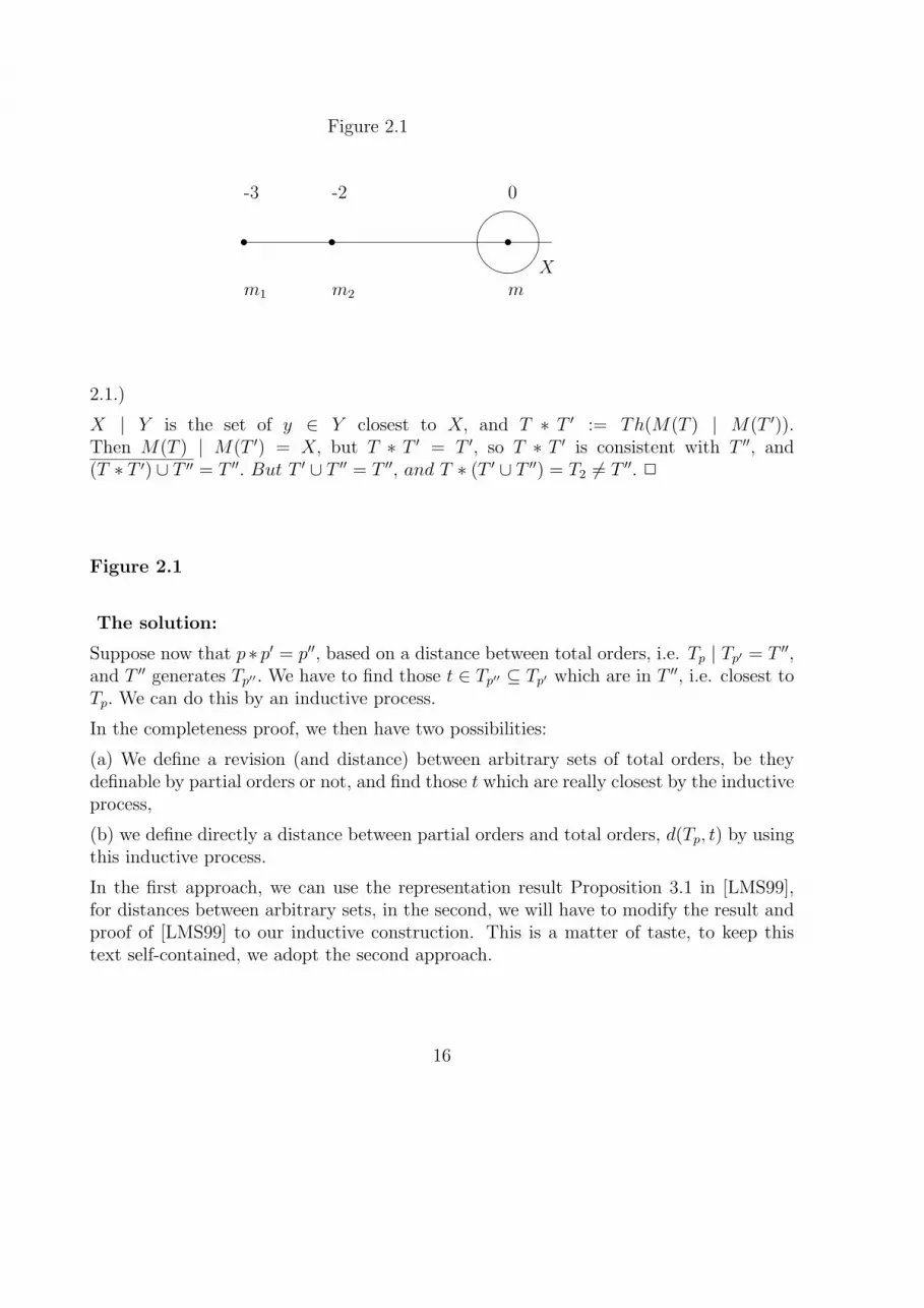
Figure 2.1

s s s&%

'$-3 -2 0

m1 m2 mX

2.1.)

X | Y is the set of y ∈ Y closest to X, and T ∗ T ′ := Th(M(T ) | M(T ′)).Then M(T ) | M(T ′) = X, but T ∗ T ′ = T ′, so T ∗ T ′ is consistent with T ′′, and(T ∗ T ′) ∪ T ′′ = T ′′. But T ′ ∪ T ′′ = T ′′, and T ∗ (T ′ ∪ T ′′) = T2 6= T ′′. 2

Figure 2.1

The solution:

Suppose now that p ∗ p′ = p′′, based on a distance between total orders, i.e. Tp | Tp′ = T ′′,and T ′′ generates Tp′′ . We have to find those t ∈ Tp′′ ⊆ Tp′ which are in T ′′, i.e. closest toTp. We can do this by an inductive process.

In the completeness proof, we then have two possibilities:

(a) We define a revision (and distance) between arbitrary sets of total orders, be theydefinable by partial orders or not, and find those t which are really closest by the inductiveprocess,

(b) we define directly a distance between partial orders and total orders, d(Tp, t) by usingthis inductive process.

In the first approach, we can use the representation result Proposition 3.1 in [LMS99],for distances between arbitrary sets, in the second, we will have to modify the result andproof of [LMS99] to our inductive construction. This is a matter of taste, to keep thistext self-contained, we adopt the second approach.

16

3 THE FORMAL RESULTS

We give a representation result for partial orders, which can be translated to logic in astraightforward way.

3.1 Proof Strategy

This paragraph gives a short outline of our proof. The reader might perhaps best readthis paragraph superficially, then the proof in detail, and finally re-read this introductionto have an overall idea of the proof.

Consider p ∗ p′.

We first identify a subset µp(p′) of Tp′ which must be the set of those elements of Tp′ which

are closest to (some element of) Tp, if ∗ is determined by a distance. The construction ofthe relation assures that all elements of µp(p

′) will have minimal distance from TP , andall other elements in Tp′ non-minimal distance from Tp. A loop condition guarantees thatwe can extend the relation to a cycle-free ranked relation, which defines the distance d tobe constructed. It is then easy to see that µp(p

′) = µdp(p

′). Condition (R3) assures thatµp(p

′) generates p ∗ p′, i.e. P (µp(p′)) = p ∗ p′, which, together with µd

p(p′) = µp(p

′), provesrepresentation.

We identify the (pseudo-) distance between Tp and Tp′ , (Tp, Tp′) with the distance betweenTp and any t′ ∈ µp(p

′), (Tp, t′) and set (Tp, Tp′) ≺ (Tp, t

′) for any t′ ∈ Tp′ − µp(p′). We

postulate a loop condition, i.e. the relations ≺ / ≈ have to be free from cycles involving≺ . If this loop condition holds, we take the ≈-equivalence classes and embed the resultingrelation between equivalence classes into a strict total order. d(t, t′) will be [(t, t′)]≈ etc.

It is easy to see that the conditions of Proposition 3.3 hold, if ∗ is defined by a distance.In particular, it is routine work to check by induction that µp(p

′) is exactly the set oft′ ∈ Tp′ closest to Tp. The necessary arguments are given as comments in the constructionof µp(p

′).

For the converse: Set µdp(p

′) := {t ∈ Tp′ : ∃s ∈ Tp∀s′ ∈ Tp∀t′ ∈ Tp′(d(s, t) ≤ d(s′, t′))}. Itsuffices to show µd

p(p′) = µp(p

′), as by condition (R3) P (µp(p′)) = p ∗ p′, so p ∗ p′ = p ∗d p′

follows (∗d is the revision generated by the distance d).

We conclude by a comparison to the completeness proofs for revision in [LMS99]: We haveconcentrated here on the problem of non-definable sets, which complicate our situation(and conditions) in comparison with those of [LMS99]. Identifying d(Tp, Tp′) with d(Tp, t

′)for any t′ ∈ µp(p

′) facilitates the later parts of the completeness proof. Note that a similarstrategy to construct the closest elements in the infinite case of [LMS99] would avoid thedefinability preservation condition (see Proposition 3.1 and Example 3.1 there) - at theprice of complicating the conditions and the construction of the relation.

17

3.2 The inductive search for closest elements

Let Y be a finite set of size n. t ∈ T contains n ∗ (n− 1)/2 pairs of elements from Y. Wethus define:

Definition 3.1

Let Y have finite size n. p ∈ P has weakness w(p) := n ∗ (n− 1)/2− card(p).

Thus, a total order has weakness 0, the next strongest has weakness 1, i.e. for just onepair z, z′ the relation is undefined, etc.

We want to determine the total orders containing p′, closest to Tp. As argued above, itis usually insufficient to consider just p ∗ p′. We will consider additionally p ∗ p′′, wherep′ ⊆ p′′, with p′′ of increasing weakness. µp(p

′) will be the set of total orders t ∈ Tp′ , whichare closest to Tp.

Remark 3.1

Let t ∈ Tp′ . Then there is at most one t′ ∈ Tp′ s.t. there is no p′′, p′ ⊂ p′′, t, t′ ∈ Tp′′ .

Proof:

The only possible candidate for t′ is the total order which agrees with t on p′, and disagreeseverywhere else, we denote this t′ by t− - if it exists. (The p′ relative to which t− isconstructed will be clear from the context). All other t′ agree with t on more thancard(p′) pairs, so they are contained in some p′′ stronger than p′.

(Remark: If < is an arbitrary relation, there is one such t′. If we look only at acyclicrelations, this need not be the case: Let Y := {a, b, c}, p := {a > b}, t := {a > c > b}(we have added a > c, c > b), t− = {a > b, b > c, c > a} is not an acyclic relation.) 2

Construction 3.1

Construction of the relations ≺ and ≈ between sets of total orders, and of the sets µp(p′).

(We will identify singletons with their elements to keep notation simple.)

The construction will simultaneously show:

(α) for t, t′ ∈ µp(p′) (Tp, t) ≈∗ (Tp, t

′),

(β) for t′ ∈ µp(p′), t ∈ Tp′ − µp(p

′) (Tp, t′) ≺∗ (Tp, t),

(γ) µp(p′) 6= ∅.

(Here and in the following, ≈∗ will be the transitive closure of ≈, ≺∗ the transitive closureof ≈ and ≺, involving at least once ≺, etc.)

18

Case 0, w(p′) = 0:

This will give no information, as Tp′ contains exactly one element, p′. Set µp(p′) := {p′}.

Case 1, w(p′) = 1:

Then Tp′ = {t, t′}, where t and t′ agree, except for one pair.

If p ∗ p′ = t, then (Tp, t) ≺ (Tp, t′), µp(p

′) := {t}.If p ∗ p′ = t′, then (Tp, t

′) ≺ (Tp, t), µp(p′) := {t′}.

If p ∗ p′ = p′, then (Tp, t) ≈ (Tp, t′), µp(p

′) := {t, t′}.

Case w(p′) = n → w(p′) = n + 1:

Let p ∗ p′ := p+.

Comment: First, any t ∈ Tp′ − Tp+ must have non-minimal distance from Tp. Second,some, perhaps not all, t ∈ Tp+ will have minimal distance from Tp. We have to identifythose, i.e. the set µp(p

′), and µp(p′) will have to generate p+.

Let now p′′ be s.t. p′ ⊂ p′′. By induction hypothesis, we have determined those t′′ ∈ Tp′′

which have minimal distance from Tp in Tp′′ , i.e. µp(p′′). We determine now those t ∈ Tp′

which have minimal distance from Tp, i.e. we examine whether t ∈ µp(p′), and will in

some cases add new pairs to the relations ≺ / ≈ .

Comment: If t does not have minimal distance to Tp in all p′′ s.t. t ∈ Tp′′ and p′ ⊂ p′′, thent cannot have minimal distance in Tp′ (global minima have to be local minima). Thus,such t are not in µp(p

′).

So suppose t is a local minimum in all such Tp′′ .

The only t′′ we cannot compare locally - i.e. through p ∗ p′′ with t, t′′ ∈ Tp′′ , p′ ⊂ p′′ - to tis t− - if it exists.

Case (a): t− is not a local minimum in all p′′ s.t. p′ ⊂ p′′.

Then, by (β) and (γ) for the induction hypothesis, there is such p′′ with (Tp, t′′) ≺∗ (Tp, t

−)for some t′′ ∈ Tp′′ . But there is p0 s.t. p′ ⊂ p0, t, t′′ ∈ Tp0 (by uniqueness of t−), and byprerequisite and (α) and (β) for p0 (Tp, t) ¹∗ (Tp, t

′′). We put t into µp(p′).

Case (b): t− is a local minimum everywhere, too.

Case (b.a), there is t′′ s.t. t′′ 6= t, t′′ 6= t−, (Tp, t) ≈∗ (Tp, t′′): Note that there is p′′ s.t.

p′ ⊂ p′′, t−, t′′ ∈ Tp′′ (as (t−)− = t).

Case (b.a.1) If t′′ ∈ µp(p′′), then (Tp, t) ≈∗ (Tp, t

′′) ≈ (Tp, t−). We then put t into µp(p

′).

Case (b.a.2) If t′′ 6∈ µp(p′′), then (Tp, t

−) ≺∗ (Tp, t′′) ≈∗ (Tp, t). We then do NOT put t

into µp(p′).

19

Case (b.b), there is t′′ 6= t, t′′ 6= t− s.t. (Tp, t−) ≈ (Tp, t

′′): Analogous.

Case (b.c), both t and t− have (strictly) smallest distance from Tp in all Tp′′ with p′ ⊂ p′′

which contain them. Then:

set (Tp, t) ≈ (Tp, t−) and µp(p

′) := {t, t−}, if p ∗ p′ = p′,

set (Tp, t) ≺ (Tp, t−) and µp(p

′) := {t}, if p ∗ p′ = t,

set (Tp, t−) ≺ (Tp, t) and µp(p

′) := {t−}, if p ∗ p′ = t .

Note that only in Case (b.c) we have added new pairs to ≈ and ≺ .

Finally, set for any t ∈ µp(p′) (Tp, Tp′) ≈ (Tp, t), consequently by (α) and (β) for any

t′′ ∈ Tp′ − µp(p′) (Tp, Tp′) ≺∗ (Tp, t

′′). 2

3.3 The representation result

Condition 3.1

Let ∗ be a function ∗ : P × P → P . Consider the conditions:

(R0) p′ ⊆ (p ∗ p′),

(R1) Tp ∩ Tp′ 6= ∅ → p ∗ p′ = p ∪ p′,

(R2) the relation ≺ / ≈ as constructed in Construction 3.1, and closed under (Tp, Tp′) ≈(Tp′ , Tp) (i.e. symmetry) is free from cycles involving ≺,

(R3) µp(p′) as constructed in Construction 3.1 generates p ∗ p′, i.e. P (µp(p

′)) = p ∗ p′.

Assume henceforth ≈ to be closed under symmetry.

Fact 3.2

The conditions (Ri) entail:

(a) (t, t) ≺ (t, t′) for any t, t′ with t 6= t′,

(b) (t, t) ≈∗ (t′, t′) for any t, t′.

Proof:

(a) is trivial, consider t ∗ p where p ⊆ t, t′. (By above construction, µt(p) = {t}).(b) is trivial, consider p ∗ p where p ⊆ t, t′. (By above construction, t, t′ ∈ µp(p). Thus(Tp, t

′) ≈ (Tp, Tp) ≈ (Tp, t). Moreover t∗p = t, so (t, Tp) ≈ (t, t). Likewise (t′, Tp) ≈ (t′, t′).)2

20

Proposition 3.3

Let Y be a finite set, P and T as defined in Definition 2.11, ∗ : P × P → P .

If ∗ is defined by a symmetric distance i.e. p ∗ p′ = P( {t ∈ Tp′ : ∃s ∈ Tp∀s′ ∈ Tp∀t′ ∈Tp′(d(s, t) ≤ d(s′, t′))} ), then the conditions (Ri) of Condition 3.1 hold for ∗, the relations≺ / ≈ defined in Construction 3.1.

Conversely, if the conditions (Ri) of Condition 3.1 hold for ∗, the relations ≺ / ≈ definedin Construction 3.1, ∗ can be represented by a symmetric distance over T.

Proof:

“→” is easy: The Construction 3.1 determines the closest elements, if ∗ is defined by adistance, so (R3) in Condition 3.1 holds. Closure under symmetry will preserve acyclicity,so (R2) holds. As d(t, t) = 0, and d(t, t′) > 0 for t 6= t′, and by Fact 2.2 (c) and (d), (R1)holds. Finally, (R0) will trivially hold.

We turn to “←”.

Standard arguments about orders show that the following construction is possible: Embed≺ into a total order, set d(x, y) := [(x, y)]≈ (i.e. its equivalence class), respecting ≺∗, and¹∗, i.e. (x, y) ≺∗ (x′, y′) → d(x, y) < d(x′, y′), and (x, y) ¹∗ (x′, y′) → d(x, y) ≤ d(x′, y′).

0 := [(t, t)]≈ for any t does what it should do: 0 is well-defined by Fact 3.2 (b), and strictlysmaller than any (t, t′), t 6= t′, by Fact 3.2 (a).

We first note:

(a) t ∈ Tp′ − µp(p′) → ∃s′ ∈ Tp∃t′ ∈ Tp′∀s ∈ Tp(s

′, t′) ≺∗ (s, t),

(b) t ∈ µp(p′) → ∃s ∈ Tp∀s′ ∈ Tp∀t′ ∈ Tp′(s, t) ¹∗ (s′, t′).

Proof: (a) Let t′ ∈ µp(p′), s′ ∈ µt′(p), then (s′, t′) ¹ (Tp, t

′) ≺ (Tp, t) ¹ (s, t).

(b) Let s ∈ µt(p), then (s, t) ¹ (Tp, t) ¹ (Tp, Tp′) ¹ (Tp, t′) ¹ (s′, t′).

We now show p ∗ p′ = p ∗d p′. By Condition 3.1, (R3), it suffices to show µp(p′) = µd

p(p′),

where µdp(p

′) := {t ∈ Tp′ : ∃s ∈ Tp∀s′ ∈ Tp∀t′ ∈ Tp′(d(s, t) ≤ d(s′, t′))}. (The result followsby p ∗ p′ = P (µp(p

′)), and p ∗d p′ := P (µdp(p

′)).)

“⊇”: Let t ∈ Tp′ − µp(p′), so by (a) t 6∈ µd

p(p′).

“⊆”: Suppose t ∈ Tp′ , t ∈ µp(p′), but t 6∈ µd

p(p′). Choose s ∈ Tp s.t. for no s′′ ∈ Tp

d(s′′, t) < d(s, t). This exists, as Tp is finite, and by the fact that < is free from cycles.By t 6∈ µd

p(p′), there is s′ ∈ Tp, t′ ∈ Tp′ s.t. d(s′, t′) < d(s, t). As t ∈ µp(p

′), there is by (b)s′′ ∈ Tp with (s′′, t) ¹∗ (s′, t′), so d(s′′, t) ≤ d(s′, t′). Thus, d(s′′, t) ≤ d(s′, t′) < d(s, t), acontradiction to the choice of s. 2

21

3.4 Discussion of the AGM postulates

For easier comparison, we adopt here the classical AGM notation.

We conclude with a discussion of the AGM postulates. The arguments will be valid forboth approaches.

(K ∗ 1) and (K ∗ 6) have no very close analogue here. (However: as we took standardrepresentations of logics, something like (K ∗6) holds automatically, and the thing closestto (K ∗ 1) is preservation of the properties (Pi), which was discussed above.)

(K ∗ 2) holds, as we choose among the total orders compatible with ∼| ′.

(K ∗3) and (K ∗4) correspond to the respect of 0 - (R1) in Condition 3.1. More precisely,(K ∗ 3) + (K ∗ 4) say that, if K ∪ {A} is consistent, then K ∗A is (the deductive closureof) K ∪{A}. Semantically speaking, this means that, if M(K)∩M(A) 6= ∅, then K ∗A =Th(M(K)∩M(A)) - where M(T ) is the set of models of a theory T, and Th(X) the set offormulas valid in a set of models X. If we base revision on a distance between models asabove, then this corresponds to the fact that M(K) ∩M(A) contains exactly the modelsof A of distance 0 from M(K).

(K ∗ 5) : We consider only nonempty sets, and, for any two finite sets X, Y, the set ofelements of Y closest to X is non-empty.

(K ∗ 7) and (K ∗ 8) will not hold, by the definability problem, consider e.g. the followingsituation: Let p′ ⊆ p′′, consider (p∗p′)∪p′′ and p∗ (p′∪p′′). Let the closest elements of Tp′

to Tp be t0 and t1 , the closest element of Tp′′ to Tp be t2, and let t0∩ t1 ⊆ t3 ∈ Tp′′ , t2 6= t3.Thus, t3 extends p′′, and is in the set generated by the elements of Tp′ , closest to Tp. Assumemoreover that t3 is the only t ∈ Tp′′ , which is in this set. Such an arrangement is possible,as we can choose the distance ad libitum. Then T(p∗p′)∪p′′ = {t3}, but Tp∗(p′∪p′′) = {t2}, so(K ∗ 7) and (K ∗ 8) both fail. Again, this comes as no surprise.

4 CONCLUSION AND FUTURE WORK

We first argued for the relevance of revising defeasible databases. We then gave an abstractanalysis of AGM revision in terms of choice functions on sets of models, which makes theconnection to preferential models immediate and also shows how to do revision on otherobjects than theories and formulas. We treated logics as partial orders, correspondingto sets of total orders, and revision choice functions choose among those total orders,strengthening the second logic. The choice functions themselves were determined by adistance between those total orders, which also gives us a semantics for our approach.

22

The main technical problem with a representation result is a definability problem: partialorders define only very few sets of total orders, even in the finite case. We solved thisdifficulty by an inductive construction of closest elements of ever coarser partial orders.

A basically similar approach and strategies should also work for updating defeasible infor-mation under some maximal inertia assumption (as discussed for the classical frameworke.g. in [LMS99]).

Our analysis of revision in terms of choice functions makes a semantical approach toDarwiche/Pearl style revision of conditional theories immediate. We have not pursuedthis any further.

It also leads to the conjecture that duplicating models might free us from the mixedleft and right hand conditions for distance based semantics of e.g. [LMS99], which areessentially conditions interconnecting distances from different starting points. To pursuethe ideas of [SM94] seems promising: We have merged there several metrics into one singlemetric using multiplication of models.

References

[AGM85] C.Alchourron, P.Gardenfors, D.Makinson, “On the Logic of Theory Change:Partial Meet Contraction and Revision Functions”, Journal of Symbolic Logic50 (1985), pp. 510-530

[BB94] Shai Ben-David, R.Ben-Eliahu, “A modal logic for subjective default reasoning”,Proceedings LICS-94, 1994

[DP97] A.Darwiche, J.Pearl, “On the logic of iterated belief revision”, Artificial Intelli-gence 89 (1997), pp. 1-29

[FH95] N.Friedman, J.Halpern, “Plausibility Measures and Default Reasoning”, IBMAlmaden Research Center Tech.Rept. 1995

[Gab85] D.M.Gabbay, “Theoretical foundations for non-monotonic reasoning in expertsystems”. In: K.R.Apt (ed.), “Logics and Models of Concurrent Systems”,Springer, Berlin, 1985, pp. 439-457

[Gar88] P.Gardenfors, “Knowledge in Flux”, MIT Press, 1988

[KLM90] S.Kraus, D.Lehmann, M.Magidor, “Nonmonotonic Reasoning, PreferentialModels and Cumulative Logics”, Artificial Intelligence 44 (1990), pp. 167-207

[LM92] D.Lehmann, M.Magidor, “What does a conditional knowledge base entail?”,Artificial Intelligence 55 (1992), pp. 1-60

23

[Mak93] D.Makinson, “Five Faces of Minimality”, Studia Logica 52 (1993), pp. 339-379

[Mak94] D.Makinson, “General patterns in nonmonotonic reasoning”, in D.Gabbay,C.Hogger, Robinson (eds.), “Handbook of Logic in Artificial Intelligence andLogic Programming”, vol. III: “Nonmonotonic and Uncertain Reasoning”, Ox-ford University Press, 1994, pp. 35-110

[Sch92] K.Schlechta: “Some Results on Classical Preferential Models”, Journal of Logicand Computation, Oxford, Vol. 2, No. 6, pp. 675-686, 1992

[Sch96] K.Schlechta: “Some Completeness Results for Stoppered and Ranked ClassicalPreferential Models”, Journal of Logic and Computation, Oxford, Vol. 6, No. 4,pp. 599-622, 1996

[Sch97] K.Schlechta: “Filters and Partial Orders”, Journal of the Interest Group in Pureand Applied Logics, Vol. 5, No. 5, pp. 753-772, 1997

[LMS99] D.Lehmann, M.Magidor, K.Schlechta: “Distance Semantics for Belief Revision”,to appear in Journal of Symbolic Logic

[SLM96] K.Schlechta, D.Lehmann, M.Magidor: “Distance Semantics for Belief Revision”,in Proceedings of: Theoretical Aspects of Rationality and Knowledge, Tark VI,1996, ed. Y.Shoham, Morgan Kaufmann, San Francisco, 1996, pp. 137-145

[SM94] K.Schlechta, D.Makinson: “Local and Global Metrics for the Semantics of Coun-terfactual Conditionals”, Journal of Applied Non-Classical Logics, Vol.4, No.2,pp. 129-140, Hermes, Paris, 1994

24