Embed Size (px)
Citation preview
How to Contact The MathWorks:
www.mathworks.com Webcomp.soft-sys.matlab Newsgroup
[email protected] Product enhancement [email protected] Bug [email protected] Documentation error reports
ISBN 0-9755787-6-6
Learning MATLAB© COPYRIGHT 1984 - 2005 by The MathWorks, Inc. The software described in this document is furnished under a license agreement. The software may be used or copied only under the terms of the license agreement. No part of this manual may be photocopied or repro-duced in any form without prior written consent from The MathWorks, Inc.
FEDERAL ACQUISITION: This provision applies to all acquisitions of the Program and Documentation by, for, or through the federal government of the United States. By accepting delivery of the Program or Documentation, the government hereby agrees that this software or documentation qualifies as commercial computer software or commercial computer software documentation as such terms are used or defined in FAR 12.212, DFARS Part 227.72, and DFARS 252.227-7014. Accordingly, the terms and conditions of this Agreement and only those rights specified in this Agreement, shall pertain to and govern the use, modification, reproduction, release, performance, display, and disclosure of the Program and Documentation by the federal government (or other entity acquiring for or through the federal government) and shall supersede any conflicting contractual terms or conditions. If this License fails to meet the government's needs or is inconsistent in any respect with federal procurement law, the government agrees to return the Program and Documentation, unused, to The MathWorks, Inc.
TrademarksMATLAB, Simulink, Stateflow, Handle Graphics, Real-Time Workshop, and xPC TargetBox are registered trademarks of The MathWorks, Inc. Other product or brand names are trademarks or registered trademarks of their respective holders.
PatentsThe MathWorks products are protected by one or more U.S. patents. Please see www.mathworks.com/patents for more information.
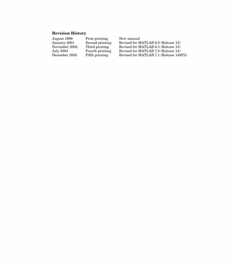
Revision HistoryAugust 1999 First printing New manualJanuary 2001 Second printing Revised for MATLAB 6.0 (Release 12)November 2002 Third printing Revised for MATLAB 6.5 (Release 13)July 2004 Fourth printing Revised for MATLAB 7.0 (Release 14)December 2005 Fifth printing Revised for MATLAB 7.1 (Release 14SP3)

Contents
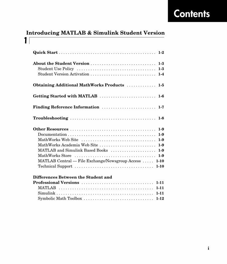
1Introducing MATLAB & Simulink Student Version
Quick Start . . . . . . . . . . . . . . . . . . . . . . . . . . . . . . . . . . . . . . . . . . . 1-2
About the Student Version . . . . . . . . . . . . . . . . . . . . . . . . . . . . . 1-3Student Use Policy . . . . . . . . . . . . . . . . . . . . . . . . . . . . . . . . . . . 1-3Student Version Activation . . . . . . . . . . . . . . . . . . . . . . . . . . . . . 1-4
Obtaining Additional MathWorks Products . . . . . . . . . . . . . 1-5
Getting Started with MATLAB . . . . . . . . . . . . . . . . . . . . . . . . . 1-6
Finding Reference Information . . . . . . . . . . . . . . . . . . . . . . . . 1-7
Troubleshooting . . . . . . . . . . . . . . . . . . . . . . . . . . . . . . . . . . . . . . 1-8
Other Resources . . . . . . . . . . . . . . . . . . . . . . . . . . . . . . . . . . . . . . 1-9Documentation . . . . . . . . . . . . . . . . . . . . . . . . . . . . . . . . . . . . . . . 1-9MathWorks Web Site . . . . . . . . . . . . . . . . . . . . . . . . . . . . . . . . . 1-9MathWorks Academia Web Site . . . . . . . . . . . . . . . . . . . . . . . . . 1-9MATLAB and Simulink Based Books . . . . . . . . . . . . . . . . . . . . 1-9MathWorks Store . . . . . . . . . . . . . . . . . . . . . . . . . . . . . . . . . . . . 1-9MATLAB Central — File Exchange/Newsgroup Access . . . . . 1-10Technical Support . . . . . . . . . . . . . . . . . . . . . . . . . . . . . . . . . . . 1-10
Differences Between the Student and Professional Versions . . . . . . . . . . . . . . . . . . . . . . . . . . . . . . . . 1-11
MATLAB . . . . . . . . . . . . . . . . . . . . . . . . . . . . . . . . . . . . . . . . . . 1-11Simulink . . . . . . . . . . . . . . . . . . . . . . . . . . . . . . . . . . . . . . . . . . . 1-11Symbolic Math Toolbox . . . . . . . . . . . . . . . . . . . . . . . . . . . . . . . 1-12
i
ii Contents
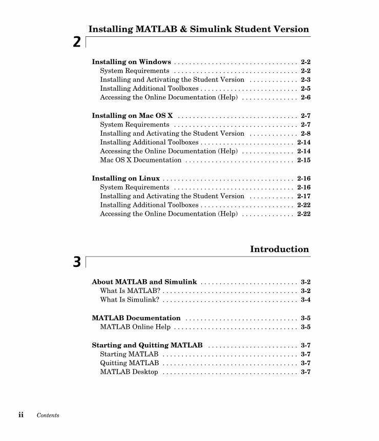
2Installing MATLAB & Simulink Student Version
Installing on Windows . . . . . . . . . . . . . . . . . . . . . . . . . . . . . . . . . 2-2System Requirements . . . . . . . . . . . . . . . . . . . . . . . . . . . . . . . . . 2-2Installing and Activating the Student Version . . . . . . . . . . . . . 2-3Installing Additional Toolboxes . . . . . . . . . . . . . . . . . . . . . . . . . . 2-5Accessing the Online Documentation (Help) . . . . . . . . . . . . . . . 2-6
Installing on Mac OS X . . . . . . . . . . . . . . . . . . . . . . . . . . . . . . . . 2-7System Requirements . . . . . . . . . . . . . . . . . . . . . . . . . . . . . . . . . 2-7Installing and Activating the Student Version . . . . . . . . . . . . . 2-8Installing Additional Toolboxes . . . . . . . . . . . . . . . . . . . . . . . . . 2-14Accessing the Online Documentation (Help) . . . . . . . . . . . . . . 2-14Mac OS X Documentation . . . . . . . . . . . . . . . . . . . . . . . . . . . . . 2-15
Installing on Linux . . . . . . . . . . . . . . . . . . . . . . . . . . . . . . . . . . . 2-16System Requirements . . . . . . . . . . . . . . . . . . . . . . . . . . . . . . . . 2-16Installing and Activating the Student Version . . . . . . . . . . . . 2-17Installing Additional Toolboxes . . . . . . . . . . . . . . . . . . . . . . . . . 2-22Accessing the Online Documentation (Help) . . . . . . . . . . . . . . 2-22
3Introduction
About MATLAB and Simulink . . . . . . . . . . . . . . . . . . . . . . . . . . 3-2What Is MATLAB? . . . . . . . . . . . . . . . . . . . . . . . . . . . . . . . . . . . . 3-2What Is Simulink? . . . . . . . . . . . . . . . . . . . . . . . . . . . . . . . . . . . . 3-4
MATLAB Documentation . . . . . . . . . . . . . . . . . . . . . . . . . . . . . . 3-5MATLAB Online Help . . . . . . . . . . . . . . . . . . . . . . . . . . . . . . . . . 3-5
Starting and Quitting MATLAB . . . . . . . . . . . . . . . . . . . . . . . . 3-7Starting MATLAB . . . . . . . . . . . . . . . . . . . . . . . . . . . . . . . . . . . . 3-7Quitting MATLAB . . . . . . . . . . . . . . . . . . . . . . . . . . . . . . . . . . . . 3-7MATLAB Desktop . . . . . . . . . . . . . . . . . . . . . . . . . . . . . . . . . . . . 3-7
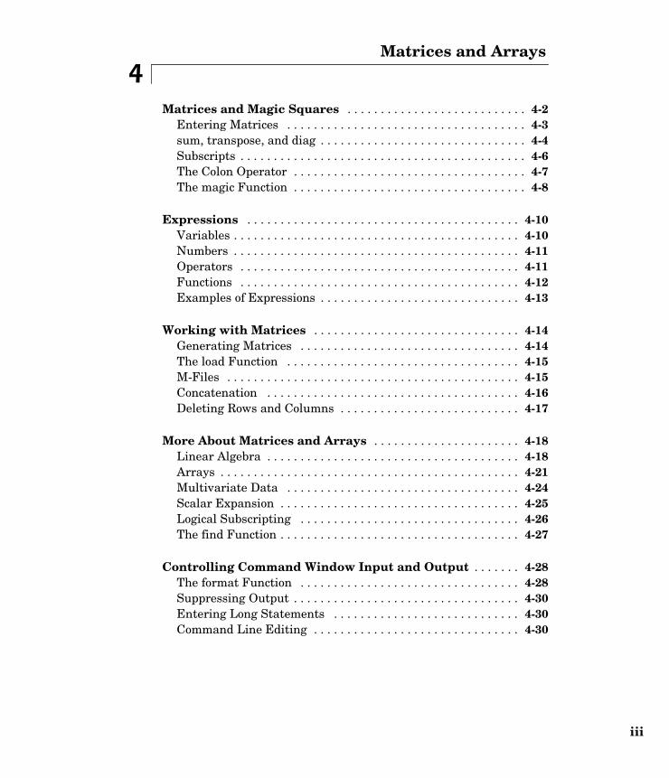
4Matrices and Arrays
Matrices and Magic Squares . . . . . . . . . . . . . . . . . . . . . . . . . . . 4-2Entering Matrices . . . . . . . . . . . . . . . . . . . . . . . . . . . . . . . . . . . . 4-3sum, transpose, and diag . . . . . . . . . . . . . . . . . . . . . . . . . . . . . . . 4-4Subscripts . . . . . . . . . . . . . . . . . . . . . . . . . . . . . . . . . . . . . . . . . . . 4-6The Colon Operator . . . . . . . . . . . . . . . . . . . . . . . . . . . . . . . . . . . 4-7The magic Function . . . . . . . . . . . . . . . . . . . . . . . . . . . . . . . . . . . 4-8
Expressions . . . . . . . . . . . . . . . . . . . . . . . . . . . . . . . . . . . . . . . . . 4-10Variables . . . . . . . . . . . . . . . . . . . . . . . . . . . . . . . . . . . . . . . . . . . 4-10Numbers . . . . . . . . . . . . . . . . . . . . . . . . . . . . . . . . . . . . . . . . . . . 4-11Operators . . . . . . . . . . . . . . . . . . . . . . . . . . . . . . . . . . . . . . . . . . 4-11Functions . . . . . . . . . . . . . . . . . . . . . . . . . . . . . . . . . . . . . . . . . . 4-12Examples of Expressions . . . . . . . . . . . . . . . . . . . . . . . . . . . . . . 4-13
Working with Matrices . . . . . . . . . . . . . . . . . . . . . . . . . . . . . . . 4-14Generating Matrices . . . . . . . . . . . . . . . . . . . . . . . . . . . . . . . . . 4-14The load Function . . . . . . . . . . . . . . . . . . . . . . . . . . . . . . . . . . . 4-15M-Files . . . . . . . . . . . . . . . . . . . . . . . . . . . . . . . . . . . . . . . . . . . . 4-15Concatenation . . . . . . . . . . . . . . . . . . . . . . . . . . . . . . . . . . . . . . 4-16Deleting Rows and Columns . . . . . . . . . . . . . . . . . . . . . . . . . . . 4-17
More About Matrices and Arrays . . . . . . . . . . . . . . . . . . . . . . 4-18Linear Algebra . . . . . . . . . . . . . . . . . . . . . . . . . . . . . . . . . . . . . . 4-18Arrays . . . . . . . . . . . . . . . . . . . . . . . . . . . . . . . . . . . . . . . . . . . . . 4-21Multivariate Data . . . . . . . . . . . . . . . . . . . . . . . . . . . . . . . . . . . 4-24Scalar Expansion . . . . . . . . . . . . . . . . . . . . . . . . . . . . . . . . . . . . 4-25Logical Subscripting . . . . . . . . . . . . . . . . . . . . . . . . . . . . . . . . . 4-26The find Function . . . . . . . . . . . . . . . . . . . . . . . . . . . . . . . . . . . . 4-27
Controlling Command Window Input and Output . . . . . . . 4-28The format Function . . . . . . . . . . . . . . . . . . . . . . . . . . . . . . . . . 4-28Suppressing Output . . . . . . . . . . . . . . . . . . . . . . . . . . . . . . . . . . 4-30Entering Long Statements . . . . . . . . . . . . . . . . . . . . . . . . . . . . 4-30Command Line Editing . . . . . . . . . . . . . . . . . . . . . . . . . . . . . . . 4-30
iii
iv Contents
5Graphics
Overview of MATLAB Plotting . . . . . . . . . . . . . . . . . . . . . . . . . 5-2The Plotting Process . . . . . . . . . . . . . . . . . . . . . . . . . . . . . . . . . . 5-2Graph Components . . . . . . . . . . . . . . . . . . . . . . . . . . . . . . . . . . . 5-5Figure Tools . . . . . . . . . . . . . . . . . . . . . . . . . . . . . . . . . . . . . . . . . 5-7Arranging Graphs Within a Figure . . . . . . . . . . . . . . . . . . . . . 5-13Selecting Plot Types . . . . . . . . . . . . . . . . . . . . . . . . . . . . . . . . . . 5-14
Editing Plots . . . . . . . . . . . . . . . . . . . . . . . . . . . . . . . . . . . . . . . . 5-16Plot Editing Mode . . . . . . . . . . . . . . . . . . . . . . . . . . . . . . . . . . . 5-16Using Functions to Edit Graphs . . . . . . . . . . . . . . . . . . . . . . . . 5-19
Examples — Using MATLAB Plotting Tools . . . . . . . . . . . . . 5-20Modifying the Graph Data Source . . . . . . . . . . . . . . . . . . . . . . 5-27
Preparing Graphs for Presentation . . . . . . . . . . . . . . . . . . . . 5-29Modify the Graph to Enhance the Presentation . . . . . . . . . . . 5-30Printing the Graph . . . . . . . . . . . . . . . . . . . . . . . . . . . . . . . . . . . 5-33Exporting the Graph . . . . . . . . . . . . . . . . . . . . . . . . . . . . . . . . . 5-35
Basic Plotting Functions . . . . . . . . . . . . . . . . . . . . . . . . . . . . . . 5-38Creating a Plot . . . . . . . . . . . . . . . . . . . . . . . . . . . . . . . . . . . . . . 5-38Multiple Data Sets in One Graph . . . . . . . . . . . . . . . . . . . . . . . 5-40Specifying Line Styles and Colors . . . . . . . . . . . . . . . . . . . . . . . 5-41Plotting Lines and Markers . . . . . . . . . . . . . . . . . . . . . . . . . . . . 5-41Imaginary and Complex Data . . . . . . . . . . . . . . . . . . . . . . . . . . 5-43Adding Plots to an Existing Graph . . . . . . . . . . . . . . . . . . . . . . 5-44Figure Windows . . . . . . . . . . . . . . . . . . . . . . . . . . . . . . . . . . . . . 5-46Multiple Plots in One Figure . . . . . . . . . . . . . . . . . . . . . . . . . . . 5-46Controlling the Axes . . . . . . . . . . . . . . . . . . . . . . . . . . . . . . . . . 5-48Axis Labels and Titles . . . . . . . . . . . . . . . . . . . . . . . . . . . . . . . . 5-49Saving Figures . . . . . . . . . . . . . . . . . . . . . . . . . . . . . . . . . . . . . . 5-51
Mesh and Surface Plots . . . . . . . . . . . . . . . . . . . . . . . . . . . . . . . 5-52Visualizing Functions of Two Variables . . . . . . . . . . . . . . . . . . 5-52
Images . . . . . . . . . . . . . . . . . . . . . . . . . . . . . . . . . . . . . . . . . . . . . . 5-58Reading and Writing Images . . . . . . . . . . . . . . . . . . . . . . . . . . . 5-59
Printing Graphics . . . . . . . . . . . . . . . . . . . . . . . . . . . . . . . . . . . . 5-60
Handle Graphics . . . . . . . . . . . . . . . . . . . . . . . . . . . . . . . . . . . . . 5-62Using the Handle . . . . . . . . . . . . . . . . . . . . . . . . . . . . . . . . . . . . 5-62Graphics Objects . . . . . . . . . . . . . . . . . . . . . . . . . . . . . . . . . . . . 5-63Setting Object Properties . . . . . . . . . . . . . . . . . . . . . . . . . . . . . . 5-65Specifying the Axes or Figure . . . . . . . . . . . . . . . . . . . . . . . . . . 5-68Finding the Handles of Existing Objects . . . . . . . . . . . . . . . . . 5-69
Animations . . . . . . . . . . . . . . . . . . . . . . . . . . . . . . . . . . . . . . . . . . 5-71Erase Mode Method . . . . . . . . . . . . . . . . . . . . . . . . . . . . . . . . . . 5-71Creating Movies . . . . . . . . . . . . . . . . . . . . . . . . . . . . . . . . . . . . . 5-73
6Programming
Flow Control . . . . . . . . . . . . . . . . . . . . . . . . . . . . . . . . . . . . . . . . . 6-2if . . . . . . . . . . . . . . . . . . . . . . . . . . . . . . . . . . . . . . . . . . . . . . . . . . 6-2switch and case . . . . . . . . . . . . . . . . . . . . . . . . . . . . . . . . . . . . . . 6-4for . . . . . . . . . . . . . . . . . . . . . . . . . . . . . . . . . . . . . . . . . . . . . . . . . 6-5while . . . . . . . . . . . . . . . . . . . . . . . . . . . . . . . . . . . . . . . . . . . . . . . 6-6continue . . . . . . . . . . . . . . . . . . . . . . . . . . . . . . . . . . . . . . . . . . . . 6-6break . . . . . . . . . . . . . . . . . . . . . . . . . . . . . . . . . . . . . . . . . . . . . . . 6-7try - catch . . . . . . . . . . . . . . . . . . . . . . . . . . . . . . . . . . . . . . . . . . . 6-8return . . . . . . . . . . . . . . . . . . . . . . . . . . . . . . . . . . . . . . . . . . . . . . 6-8
Other Data Structures . . . . . . . . . . . . . . . . . . . . . . . . . . . . . . . . . 6-9Multidimensional Arrays . . . . . . . . . . . . . . . . . . . . . . . . . . . . . . . 6-9Cell Arrays . . . . . . . . . . . . . . . . . . . . . . . . . . . . . . . . . . . . . . . . . 6-11Characters and Text . . . . . . . . . . . . . . . . . . . . . . . . . . . . . . . . . 6-13Structures . . . . . . . . . . . . . . . . . . . . . . . . . . . . . . . . . . . . . . . . . . 6-16
Scripts and Functions . . . . . . . . . . . . . . . . . . . . . . . . . . . . . . . . 6-19Scripts . . . . . . . . . . . . . . . . . . . . . . . . . . . . . . . . . . . . . . . . . . . . . 6-20Functions . . . . . . . . . . . . . . . . . . . . . . . . . . . . . . . . . . . . . . . . . . 6-21Types of Functions . . . . . . . . . . . . . . . . . . . . . . . . . . . . . . . . . . . 6-23Global Variables . . . . . . . . . . . . . . . . . . . . . . . . . . . . . . . . . . . . . 6-25
v
vi Contents
Passing String Arguments to Functions . . . . . . . . . . . . . . . . . . 6-26The eval Function . . . . . . . . . . . . . . . . . . . . . . . . . . . . . . . . . . . 6-27Function Handles . . . . . . . . . . . . . . . . . . . . . . . . . . . . . . . . . . . . 6-28Function Functions . . . . . . . . . . . . . . . . . . . . . . . . . . . . . . . . . . 6-28Vectorization . . . . . . . . . . . . . . . . . . . . . . . . . . . . . . . . . . . . . . . 6-31Preallocation . . . . . . . . . . . . . . . . . . . . . . . . . . . . . . . . . . . . . . . . 6-31
7Creating Graphical User Interfaces
What Is GUIDE? . . . . . . . . . . . . . . . . . . . . . . . . . . . . . . . . . . . . . . . 7-2
Laying Out a GUI . . . . . . . . . . . . . . . . . . . . . . . . . . . . . . . . . . . . . 7-3Starting GUIDE . . . . . . . . . . . . . . . . . . . . . . . . . . . . . . . . . . . . . . 7-3The Layout Editor . . . . . . . . . . . . . . . . . . . . . . . . . . . . . . . . . . . . 7-4
Programming a GUI . . . . . . . . . . . . . . . . . . . . . . . . . . . . . . . . . . . 7-6
8Desktop Tools and Development Environment
Desktop Overview . . . . . . . . . . . . . . . . . . . . . . . . . . . . . . . . . . . . . 8-2Arranging the Desktop . . . . . . . . . . . . . . . . . . . . . . . . . . . . . . . . 8-3Start Button . . . . . . . . . . . . . . . . . . . . . . . . . . . . . . . . . . . . . . . . . 8-3
Command Window and Command History . . . . . . . . . . . . . . . 8-4Command Window . . . . . . . . . . . . . . . . . . . . . . . . . . . . . . . . . . . . 8-4Command History . . . . . . . . . . . . . . . . . . . . . . . . . . . . . . . . . . . . 8-5
Help Browser . . . . . . . . . . . . . . . . . . . . . . . . . . . . . . . . . . . . . . . . . 8-6
Current Directory Browser and Search Path . . . . . . . . . . . . 8-9Current Directory . . . . . . . . . . . . . . . . . . . . . . . . . . . . . . . . . . . . . 8-9Search Path . . . . . . . . . . . . . . . . . . . . . . . . . . . . . . . . . . . . . . . . 8-10
Workspace Browser and Array Editor . . . . . . . . . . . . . . . . . . 8-11Workspace Browser . . . . . . . . . . . . . . . . . . . . . . . . . . . . . . . . . . 8-11Array Editor . . . . . . . . . . . . . . . . . . . . . . . . . . . . . . . . . . . . . . . . 8-12
Editor/Debugger . . . . . . . . . . . . . . . . . . . . . . . . . . . . . . . . . . . . . 8-13
M-Lint Code Check and Profiler Reports . . . . . . . . . . . . . . . 8-15M-Lint Code Check Report . . . . . . . . . . . . . . . . . . . . . . . . . . . . 8-15Profiler . . . . . . . . . . . . . . . . . . . . . . . . . . . . . . . . . . . . . . . . . . . . 8-17
Other Development Environment Features . . . . . . . . . . . . . 8-18
9Introducing the Symbolic Math Toolbox
What Is the Symbolic Math Toolbox? . . . . . . . . . . . . . . . . . . . . 9-2
Symbolic Objects . . . . . . . . . . . . . . . . . . . . . . . . . . . . . . . . . . . . . . 9-3
Creating Symbolic Variables and Expressions . . . . . . . . . . . 9-5The findsym Command . . . . . . . . . . . . . . . . . . . . . . . . . . . . . . . . 9-7
The subs Command . . . . . . . . . . . . . . . . . . . . . . . . . . . . . . . . . . . 9-8The Default Symbolic Variable . . . . . . . . . . . . . . . . . . . . . . . . . . 9-9
Symbolic and Numeric Conversions . . . . . . . . . . . . . . . . . . . 9-10Constructing Real and Complex Variables . . . . . . . . . . . . . . . . 9-12Creating Abstract Functions . . . . . . . . . . . . . . . . . . . . . . . . . . . 9-13
Creating Symbolic Math Functions . . . . . . . . . . . . . . . . . . . . 9-15Using Symbolic Expressions . . . . . . . . . . . . . . . . . . . . . . . . . . . 9-15Creating an M-File . . . . . . . . . . . . . . . . . . . . . . . . . . . . . . . . . . . 9-15
vii
viii Contents
10Using the Symbolic Math Toolbox
Calculus . . . . . . . . . . . . . . . . . . . . . . . . . . . . . . . . . . . . . . . . . . . . . 10-2Differentiation . . . . . . . . . . . . . . . . . . . . . . . . . . . . . . . . . . . . . . 10-2Limits . . . . . . . . . . . . . . . . . . . . . . . . . . . . . . . . . . . . . . . . . . . . . 10-8Integration . . . . . . . . . . . . . . . . . . . . . . . . . . . . . . . . . . . . . . . . 10-11Symbolic Summation . . . . . . . . . . . . . . . . . . . . . . . . . . . . . . . . 10-18Taylor Series . . . . . . . . . . . . . . . . . . . . . . . . . . . . . . . . . . . . . . 10-18Calculus Example . . . . . . . . . . . . . . . . . . . . . . . . . . . . . . . . . . 10-20Extended Calculus Example . . . . . . . . . . . . . . . . . . . . . . . . . . 10-28
Simplifications and Substitutions . . . . . . . . . . . . . . . . . . . . 10-41Simplifications . . . . . . . . . . . . . . . . . . . . . . . . . . . . . . . . . . . . . 10-41Substitutions . . . . . . . . . . . . . . . . . . . . . . . . . . . . . . . . . . . . . . 10-50
Variable-Precision Arithmetic . . . . . . . . . . . . . . . . . . . . . . . . 10-57Overview . . . . . . . . . . . . . . . . . . . . . . . . . . . . . . . . . . . . . . . . . . 10-57Example: Using the Different Kinds of Arithmetic . . . . . . . . 10-58Another Example . . . . . . . . . . . . . . . . . . . . . . . . . . . . . . . . . . . 10-60
Linear Algebra . . . . . . . . . . . . . . . . . . . . . . . . . . . . . . . . . . . . . . 10-62Basic Algebraic Operations . . . . . . . . . . . . . . . . . . . . . . . . . . . 10-62Linear Algebraic Operations . . . . . . . . . . . . . . . . . . . . . . . . . . 10-63Eigenvalues . . . . . . . . . . . . . . . . . . . . . . . . . . . . . . . . . . . . . . . 10-67Jordan Canonical Form . . . . . . . . . . . . . . . . . . . . . . . . . . . . . . 10-73Singular Value Decomposition . . . . . . . . . . . . . . . . . . . . . . . . 10-74Eigenvalue Trajectories . . . . . . . . . . . . . . . . . . . . . . . . . . . . . . 10-77
Solving Equations . . . . . . . . . . . . . . . . . . . . . . . . . . . . . . . . . . . 10-86Solving Algebraic Equations . . . . . . . . . . . . . . . . . . . . . . . . . . 10-86Several Algebraic Equations . . . . . . . . . . . . . . . . . . . . . . . . . . 10-87Single Differential Equation . . . . . . . . . . . . . . . . . . . . . . . . . . 10-90Several Differential Equations . . . . . . . . . . . . . . . . . . . . . . . . 10-92
Index
1
Introducing MATLAB & Simulink Student VersionThis chapter introduces MATLAB & Simulink Student Version and provides resources for using it.
Quick Start (p. 1-2) Syllabus for new users of MATLAB®
About the Student Version (p. 1-3) Description of MATLAB & Simulink Student Version
Obtaining Additional MathWorks Products (p. 1-5)
How to acquire other products for use with MATLAB & Simulink Student Version
Getting Started with MATLAB (p. 1-6) Basic steps for using MATLAB
Finding Reference Information (p. 1-7) How to learn more about MATLAB and related products
Troubleshooting (p. 1-8) Getting information and reporting problems
Other Resources (p. 1-9) Additional sources of information for MATLAB & Simulink Student Version
Differences Between the Student and Professional Versions (p. 1-11)
Product differences
1 Introducing MATLAB & Simulink Student Version
1-2
Quick StartIf you need help installing the software, see Chapter 2, “Installing MATLAB & Simulink Student Version.”
At the heart of MATLAB® is a programming language you must learn before you can fully exploit its power. You can learn the basics of MATLAB quickly, and mastery comes shortly after. You will be rewarded with high-productivity, high-creativity computing power that will change the way you work.
If you are new to MATLAB, you should start by reading Chapter 4, “Matrices and Arrays.” The most important things to learn are how to enter matrices, how to use the : (colon) operator, and how to invoke functions. After you master the basics, you should read the rest of the MATLAB chapters in this book and run the demos:
• Chapter 3, “Introduction”
Introduces MATLAB and the MATLAB desktop.
• Chapter 4, “Matrices and Arrays”
Introduces matrices and arrays, how to enter and generate them, how to operate on them, and how to control Command Window input and output.
• Chapter 5, “Graphics”
Introduces MATLAB graphic capabilities and the tools that let you customize your graphs to suit your specific needs.
• Chapter 6, “Programming”
Describes how to use the MATLAB language to create scripts and functions, and manipulate data structures, such as cell arrays and multidimensional arrays.
About the Student Version
About the Student VersionMATLAB and Simulink® are the premier software packages for technical computing in education and industry. MATLAB & Simulink Student Version provides all of the features of professional MATLAB, with no limitations, and the full functionality of professional Simulink, with model sizes up to 1000 blocks. The Student Version gives you immediate access to high-performance numeric computing, modeling, and simulation power.
MATLAB allows you to focus on your course work and applications rather than on programming details. It enables you to solve many numerical problems in a fraction of the time it would take you to write a program in a lower-level language such as C, C++, or Fortran. MATLAB helps you better understand and apply concepts in applications ranging from engineering and mathematics to chemistry, biology, and economics.
Simulink is an interactive tool for modeling, simulating, and analyzing dynamic systems, including controls, signal processing, communications, and other complex systems.
The Symbolic Math Toolbox, also included with the Student Version, is based on the Maple® 8 symbolic math engine and lets you perform symbolic computations and variable-precision arithmetic.
MATLAB products are used in a broad range of industries, including automotive, aerospace, electronics, environmental, telecommunications, computer peripherals, finance, and medicine. More than one million technical professionals at the world’s most innovative technology companies, government research labs, financial institutions, and at more than 3500 universities, rely on MATLAB and Simulink as the fundamental tools for their engineering and scientific work.
Student Use PolicyThis MATLAB & Simulink Student Version License is for use in conjunction with courses offered at degree-granting institutions. The MathWorks offers this license as a special service to the student community and asks your help in seeing that its terms are not abused.
To use this Student License, you must be a student either enrolled in a degree-granting institution or participating in a continuing education program at a degree-granting educational university.
1-3
1 Introducing MATLAB & Simulink Student Version
1-4
You may not use this Student License at a company or government lab. Also, you may not use it if you are an instructor at a university, or for research, commercial, or industrial purposes. In these cases, you can acquire the appropriate professional or academic license by contacting The MathWorks.
Student Version ActivationActivation is a secure process that verifies licensed student users. This process validates the serial number and ensures that it is not used on more systems than allowed by the MathWorks End User License Agreement.
The activation technology is designed to provide an easier and more effective way for students to authenticate and use their product than prior releases of MATLAB & Simulink Student Version.
The quickest way to activate your software is to use the activation program that starts following product installation. The activation program will guide you through the activation process. Alternatively, you can activate your software on the mathworks.com Web site.
Activation requires completion of three activities:
• Provide registration information by creating a MathWorks Account.
• Provide your serial number and the Machine ID for the computer you will be installing the software on.
• For those students who did not provide proof of student status at the time of purchase, submission and verification of proof of student status is needed.
For more information on activation, see www.mathworks.com/academia/student_version/activation.html.
Obtaining Additional MathWorks Products
Obtaining Additional MathWorks ProductsMany college courses recommend MATLAB and Simulink as standard instructional software. In some cases, the courses may require particular toolboxes, blocksets, or other products. Toolboxes and blocksets are add-on products that extend MATLAB and Simulink with domain-specific capabilities. Many of these products are available for MATLAB & Simulink Student Version. You may purchase and download these additional products at special student prices from the MathWorks Store at www.mathworks.com/store.
Some of the products you can purchase include
• Bioinformatics Toolbox
• Communications Blockset
• Control System Toolbox
• Fixed-Point Toolbox
• Fuzzy Logic Toolbox
• Image Processing Toolbox
• Neural Network Toolbox
• Optimization Toolbox
• Signal Processing Toolbox
• Statistics Toolbox
• Stateflow® (A demo version of Stateflow is included with your MATLAB & Simulink Student Version.)
For an up-to-date list of available products and their product dependencies, visit the MathWorks Store.
Note The toolboxes and blocksets that are available for MATLAB & Simulink Student Version have the same functionality as the professional versions. However, the student versions of the toolboxes and blocksets will work only with the Student Version. Likewise, the professional versions of the toolboxes and blocksets will not work with the Student Version.
1-5
1 Introducing MATLAB & Simulink Student Version
1-6
Getting Started with MATLAB
What I Want What I Should Do
I need to install and activate MATLAB.
See Chapter 2, “Installing MATLAB & Simulink Student Version.”
I want to start MATLAB. (Microsoft Windows) Double-click the MATLAB icon on your desktop.
(Macintosh OS X) Double-click the MATLAB icon on your desktop.
(Linux) Enter the matlab command at the command prompt.
I’m new to MATLAB and want to learn it quickly.
Start by reading Chapter 3, “Introduction,” through Chapter 6, “Programming,” in this book. The most important things to learn are how to enter matrices, how to use the : (colon) operator, and how to invoke functions. You will also get a brief overview of graphics and programming in MATLAB. After you master the basics, you can access the rest of the documentation through the online help facility (Help).
I want to look at some samples of what you can do with MATLAB.
There are numerous demonstrations and video tutorials included with MATLAB. You can see these by clicking Demos in the Help browser or selecting Demos from the Help menu. There are demonstrations of mathematics, graphics, programming, and much more. You also will find a large selection of demos at www.mathworks.com/demos.
Finding Reference Information
Finding Reference Information
What I Want What I Should Do
I want to know how to use a specific function.
Use the online help facility (Help). To access Help, use the command helpbrowser or use the Help menu. “MATLAB Functions: Volume 1 (A-E), Volume 2 (F-O), and Volume 3 (P-Z)” are also available in PDF format from Printing the Documentation Set on the MATLAB product page.
I want to find a function for a specific purpose, but I don’t know the function name.
There are several choices:
• From Help, browse the MATLAB functions by selecting Functions — Categorical List or Functions — Alphabetical List.
• Use lookfor (e.g., lookfor inverse) from the command line.
• Use Index or Search from Help.
I want to learn about a specific topic such as sparse matrices, ordinary differential equations, or cell arrays.
Use Help to locate the appropriate sections in the MATLAB documentation, for example, MATLAB -> Mathematics -> Sparse Matrices.
I want to know what functions are available in a general area.
Use Help to view Functions — Categorical List under MATLAB. Help provides access to the reference pages for the hundreds of functions included with MATLAB.
I want to learn about the Symbolic Math Toolbox.
See Chapter 9, “Introducing the Symbolic Math Toolbox,” and Chapter 10, “Using the Symbolic Math Toolbox,” in this book. For complete descriptions of the Symbolic Math Toolbox functions, use Help and select Functions — Categorical List or Functions — Alphabetical List from the Symbolic Math Toolbox documentation.
1-7
1 Introducing MATLAB & Simulink Student Version
1-8
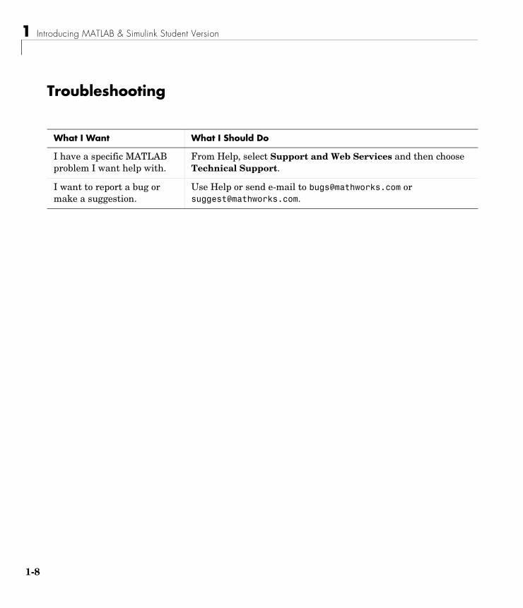
Troubleshooting
What I Want What I Should Do
I have a specific MATLAB problem I want help with.
From Help, select Support and Web Services and then choose Technical Support.
I want to report a bug or make a suggestion.
Use Help or send e-mail to [email protected] or [email protected].
Other Resources
Other Resources
DocumentationWhen you install MATLAB & Simulink Student Version on your computer, you automatically install the complete online documentation for these products. Access this documentation set from Help.
Note References to UNIX in the documentation include both Linux and Mac OS X.
Web-Based DocumentationDocumentation for all MathWorks products is online and available from the Support area of the MathWorks Web site. In addition to tutorials and function reference pages, you can find PDF versions of all the manuals.
MathWorks Web SiteAt www.mathworks.com, you’ll find information about MathWorks products and how they are used in education and industry, product demos, and MATLAB and Simulink based books.
MathWorks Academia Web SiteAt www.mathworks.com/academia, you’ll find resources for students and instructors for courses in engineering, mathematics, and science.
MATLAB and Simulink Based BooksAt www.mathworks.com/support/books, you’ll find books in many disciplines that use MATLAB and Simulink for examples and assignments.
MathWorks StoreAt www.mathworks.com/store, you can purchase add-on products and documentation.
1-9
1 Introducing MATLAB & Simulink Student Version
1-1
MATLAB Central — File Exchange/Newsgroup AccessAt www.mathworks.com/matlabcentral, you can access the MATLAB Usenet newsgroup (comp.soft-sys.matlab) as well as an extensive library of user-contributed files called the MATLAB Central File Exchange. MATLAB Central is also home to the Link Exchange where you can share your favorite links to various educational, personal, and commercial MATLAB Web sites.
The comp.soft-sys.matlab newsgroup is for professionals and students who use MATLAB and have questions or comments about it and its associated software. This is an important resource for posing questions and answering queries from other MATLAB users. MathWorks staff also participates actively in this newsgroup.
Technical SupportAt www.mathworks.com/support, you can get technical support.
Telephone and e-mail access to our technical support staff is not available for students running MATLAB & Simulink Student Version unless you are experiencing difficulty installing or downloading MATLAB or related products. There are numerous other vehicles of technical support that you can use. The “Resources and Support” section in the CD holder identifies ways to obtain additional help.
After checking the available MathWorks sources for help, if you still cannot resolve your problem, please contact your instructor. Your instructor should be able to help you. If your instructor needs assistance doing so, telephone and e-mail technical support is available to registered instructors who have adopted MATLAB & Simulink Student Version in their courses.
0
Differences Between the Student and Professional Versions
Differences Between the Student and Professional Versions
MATLABThe Student Version includes all of the features of the professional version of MATLAB.
MATLAB DifferencesThere are a few small differences between the Student Version and the professional version of MATLAB:
• The MATLAB prompt in the Student Version isEDU>>
• The window title bars include the words
<Student Version>
• Printouts contain the footerStudent Version of MATLAB
• The Check for Updates menu option on the Help menu is not available in the Student Version.
SimulinkThe Student Version contains the complete Simulink product, which is used with MATLAB to model, simulate, and analyze dynamic systems.
Simulink Differences
• Models are limited to 1000 blocks.
Note You may encounter some demos that use more than 1000 blocks. In these cases, a dialog will display stating that the block limit has been exceeded and the demo will not run.
• The window title bars include the words
<Student Version>
1-11
1 Introducing MATLAB & Simulink Student Version
1-1
• Printouts contain the footer
Student Version of MATLAB
Note The Using Simulink documentation, which is accessible from the Help browser, contains all of the information in the Learning Simulink book plus additional advanced information.
Symbolic Math ToolboxThe Symbolic Math Toolbox included with this Student Version lets you access all of the functions in the professional version of the Symbolic Math Toolbox except maple, mapleinit, and mhelp. For more information about the Symbolic Math Toolbox, see its documentation.
2
2
Installing MATLAB & Simulink Student VersionThis chapter describes how to install and activate MATLAB & Simulink Student Version.
Installing on Windows (p. 2-2) Steps to install and activate the Student Version on Microsoft Windows machines
Installing on Mac OS X (p. 2-7) Steps to install and activate the Student Version on Macintosh OS X machines
Installing on Linux (p. 2-16) Steps to install and activate the Student Version on Linux machines
2 Installing MATLAB & Simulink Student Version
2-2
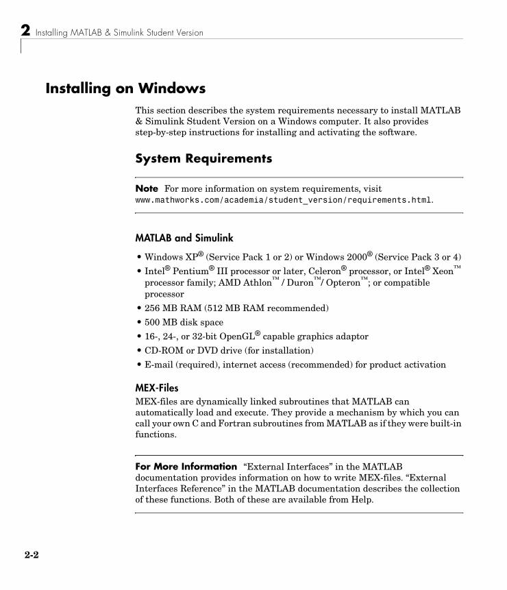
Installing on WindowsThis section describes the system requirements necessary to install MATLAB & Simulink Student Version on a Windows computer. It also provides step-by-step instructions for installing and activating the software.
System Requirements
Note For more information on system requirements, visit www.mathworks.com/academia/student_version/requirements.html.
MATLAB and Simulink
• Windows XP® (Service Pack 1 or 2) or Windows 2000® (Service Pack 3 or 4)
• Intel® Pentium® III processor or later, Celeron® processor, or Intel® Xeon™ processor family; AMD Athlon™ / Duron™/ Opteron™; or compatible processor
• 256 MB RAM (512 MB RAM recommended)
• 500 MB disk space
• 16-, 24-, or 32-bit OpenGL® capable graphics adaptor
• CD-ROM or DVD drive (for installation)
• E-mail (required), internet access (recommended) for product activation
MEX-FilesMEX-files are dynamically linked subroutines that MATLAB can automatically load and execute. They provide a mechanism by which you can call your own C and Fortran subroutines from MATLAB as if they were built-in functions.
For More Information “External Interfaces” in the MATLAB documentation provides information on how to write MEX-files. “External Interfaces Reference” in the MATLAB documentation describes the collection of these functions. Both of these are available from Help.
Installing on Windows
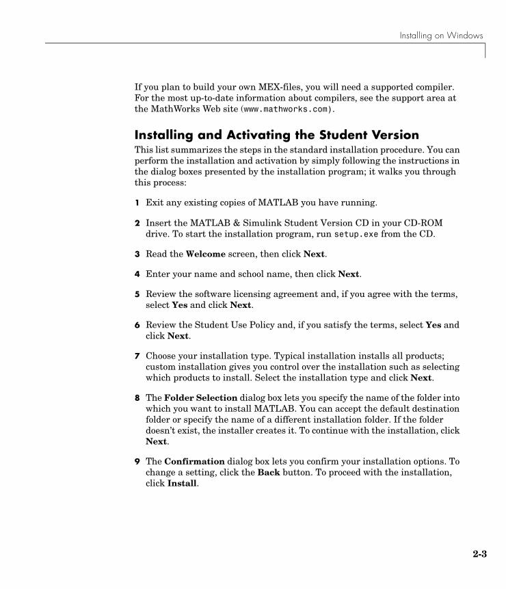
If you plan to build your own MEX-files, you will need a supported compiler. For the most up-to-date information about compilers, see the support area at the MathWorks Web site (www.mathworks.com).
Installing and Activating the Student VersionThis list summarizes the steps in the standard installation procedure. You can perform the installation and activation by simply following the instructions in the dialog boxes presented by the installation program; it walks you through this process:
1 Exit any existing copies of MATLAB you have running.
2 Insert the MATLAB & Simulink Student Version CD in your CD-ROM drive. To start the installation program, run setup.exe from the CD.
3 Read the Welcome screen, then click Next.
4 Enter your name and school name, then click Next.
5 Review the software licensing agreement and, if you agree with the terms, select Yes and click Next.
6 Review the Student Use Policy and, if you satisfy the terms, select Yes and click Next.
7 Choose your installation type. Typical installation installs all products; custom installation gives you control over the installation such as selecting which products to install. Select the installation type and click Next.
8 The Folder Selection dialog box lets you specify the name of the folder into which you want to install MATLAB. You can accept the default destination folder or specify the name of a different installation folder. If the folder doesn’t exist, the installer creates it. To continue with the installation, click Next.
9 The Confirmation dialog box lets you confirm your installation options. To change a setting, click the Back button. To proceed with the installation, click Install.
2-3
2 Installing MATLAB & Simulink Student Version
2-4
Note The installation process installs the online documentation for each product you install. This does not include documentation in PDF format, which is available only at the MathWorks Web site.
10 When the installation successfully completes, the activation process begins by displaying the Activation Overview, which describes the three steps in the process. During activation, you will:
- Enter your serial number and e-mail address.
- Provide registration information by creating a MathWorks account.
- Provide proof of student status, unless previously provided.
11 As the activation process proceeds, read the screens and enter the corresponding information. At the completion of the activation process, you will be able to use your Student Version of MATLAB & Simulink. In certain cases, your software will be temporarily activated for 30 days until your proof of student status is verified. In these cases, you will be reminded that your activation is temporary and that you need to complete the activation process. Once your proof of student status is verified, your activation is complete.
Note If you encounter a problem during the activation process, check www.mathworks.com/academia/student_version/activation.html for more information.
12 To start MATLAB, double-click the MATLAB icon that the installer creates on your desktop.
13 Customize any MATLAB environment options, if desired. For example, to specify welcome messages, default definitions, or any MATLAB expressions that you want executed every time MATLAB is invoked, create a file named startup.m in the $MATLAB\toolbox\local folder, where $MATLAB is the name of your MATLAB installation folder. Every time you start MATLAB, it executes the commands in the startup.m file.
Installing on Windows
14 Perform any additional configuration by typing the appropriate command at the MATLAB command prompt. For example, to configure the MATLAB Notebook, type notebook -setup. To configure a compiler to work with the MATLAB External Interface, type mex -setup.
For More Information The Installation Guide for Windows documentation provides additional installation information. This manual is available from Help.
Installing Additional ToolboxesTo purchase additional toolboxes, visit the MathWorks Store at www.mathworks.com/store. Once you purchase a toolbox, the product and its online documentation are downloaded to your computer.
When you download a toolbox, you receive an installation program for the toolbox. To install the toolbox and its documentation, run the installation program by double-clicking the installer icon. After you successfully install the toolbox, all of its functionality and documentation will be available to you when you start MATLAB.
2-5
2 Installing MATLAB & Simulink Student Version
2-6
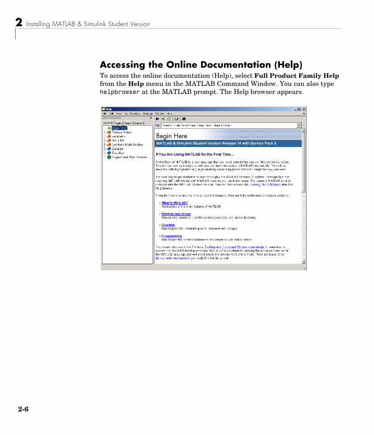
Accessing the Online Documentation (Help)To access the online documentation (Help), select Full Product Family Help from the Help menu in the MATLAB Command Window. You can also type helpbrowser at the MATLAB prompt. The Help browser appears.
Installing on Mac OS X
Installing on Mac OS XThis section describes the system requirements necessary to install MATLAB & Simulink Student Version on a Macintosh computer. It also provides step-by-step instructions for installing and activating the software.
System Requirements
Note For more information on system requirements, visit www.mathworks.com/academia/student_version/requirements.html.
MATLAB and Simulink
• Mac OS X 10.3.8, 10.3.9 (Panther™), or 10.4 (Tiger™)
• PowerPC G4 or G5 processor
• 256 MB RAM (512 MB RAM recommended)
• 500 MB disk space
• 16-bit graphics or higher adaptor and display (24-bit recommended)
• X11 (X server)
• CD-ROM or DVD drive (for installation)
• E-mail (required), internet access (recommended) for product activation
MEX-FilesMEX-files are dynamically linked subroutines that MATLAB can automatically load and execute. They provide a mechanism by which you can call your own C and Fortran subroutines from MATLAB as if they were built-in functions.
For More Information “External Interfaces” in the MATLAB documentation provides information on how to write MEX-files. “External Interfaces Reference” in the MATLAB documentation describes the collection of these functions. Both of these are available from Help.
2-7
2 Installing MATLAB & Simulink Student Version
2-8
If you plan to build your own MEX-files, you will need a supported compiler. For the most up-to-date information about compilers, see the support area at the MathWorks Web site (www.mathworks.com).
Installing and Activating the Student VersionThe following sections describe the steps you must follow to install and activate MATLAB & Simulink Student Version on a Macintosh computer.
Note If you want to install MATLAB in a particular directory, you must have the appropriate permissions. For example, to install MATLAB in the Applications directory, you must have administrator status. To create symbolic links in a particular directory, you must have the appropriate permissions. For information on setting permissions (privileges), see Macintosh Help (Command+? from the desktop).
1 Insert the MATLAB & Simulink Student Version CD in the CD-ROM drive. When the CD’s icon appears on the desktop, double-click the icon to display the CD’s contents.
2 Double-click the InstallForMacOSX icon to begin the installation.
Installing on Mac OS X
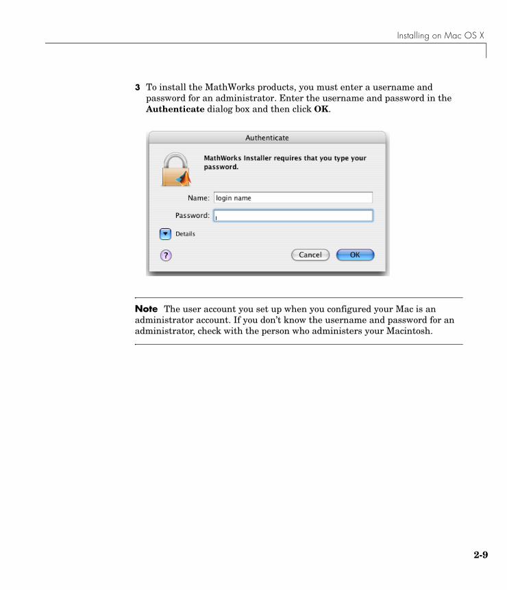
3 To install the MathWorks products, you must enter a username and password for an administrator. Enter the username and password in the Authenticate dialog box and then click OK.
Note The user account you set up when you configured your Mac is an administrator account. If you don’t know the username and password for an administrator, check with the person who administers your Macintosh.
2-9
2 Installing MATLAB & Simulink Student Version
2-1
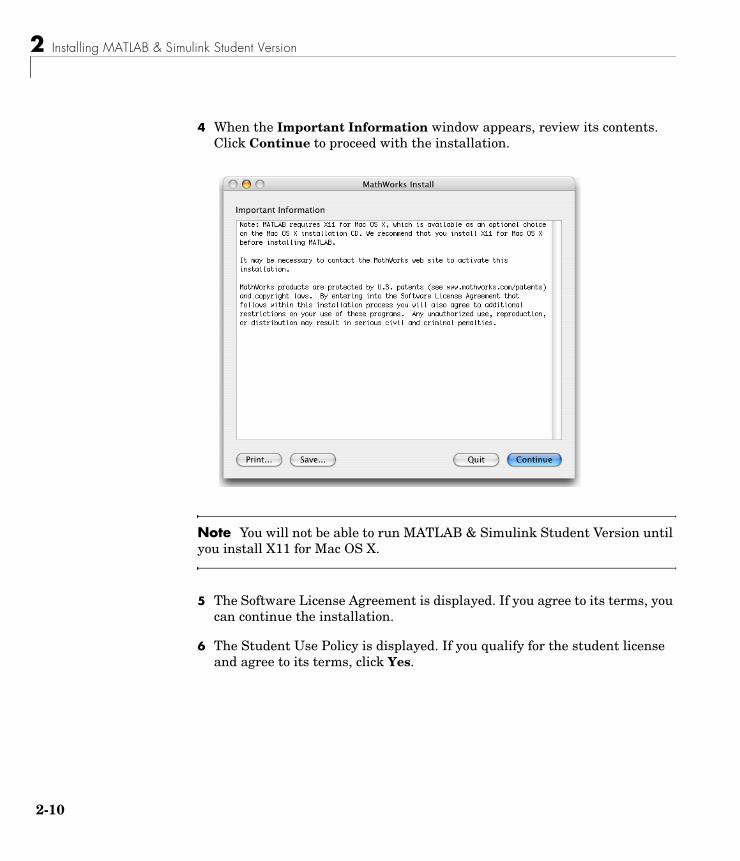
4 When the Important Information window appears, review its contents. Click Continue to proceed with the installation.
Note You will not be able to run MATLAB & Simulink Student Version until you install X11 for Mac OS X.
5 The Software License Agreement is displayed. If you agree to its terms, you can continue the installation.
6 The Student Use Policy is displayed. If you qualify for the student license and agree to its terms, click Yes.
0
Installing on Mac OS X
7 The default installation location is MATLAB_SV71 in the Applications folder on your system disk. To accept the default, click Continue. To change the location, click Choose Folder and then navigate to the desired location.
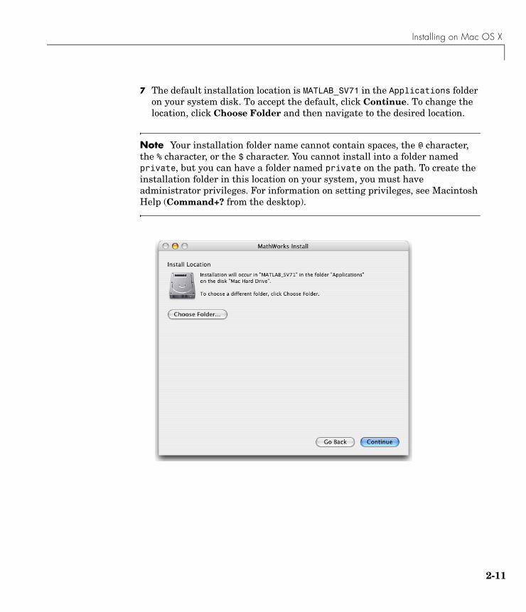
Note Your installation folder name cannot contain spaces, the @ character, the % character, or the $ character. You cannot install into a folder named private, but you can have a folder named private on the path. To create the installation folder in this location on your system, you must have administrator privileges. For information on setting privileges, see Macintosh Help (Command+? from the desktop).
2-11
2 Installing MATLAB & Simulink Student Version
2-1
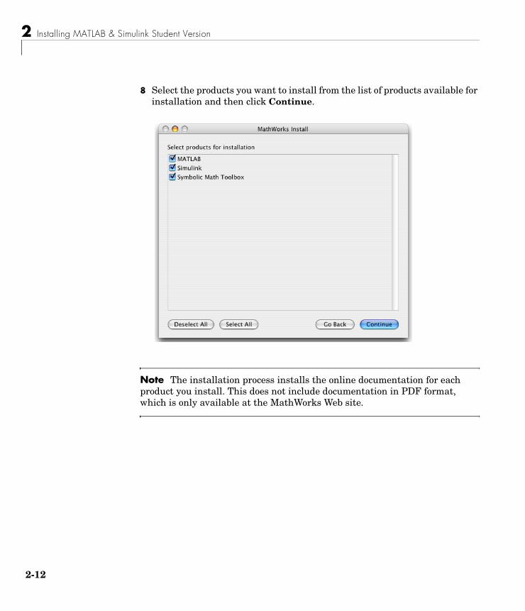
8 Select the products you want to install from the list of products available for installation and then click Continue.
Note The installation process installs the online documentation for each product you install. This does not include documentation in PDF format, which is only available at the MathWorks Web site.
2
Installing on Mac OS X
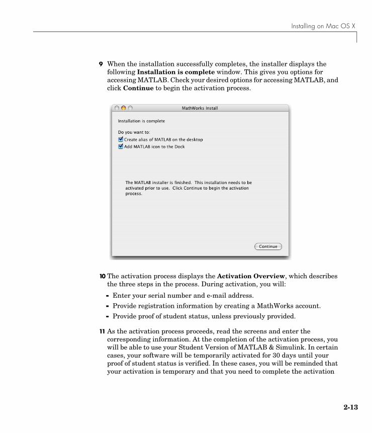
9 When the installation successfully completes, the installer displays the following Installation is complete window. This gives you options for accessing MATLAB. Check your desired options for accessing MATLAB, and click Continue to begin the activation process.
10 The activation process displays the Activation Overview, which describes the three steps in the process. During activation, you will:
- Enter your serial number and e-mail address.
- Provide registration information by creating a MathWorks account.
- Provide proof of student status, unless previously provided.
11 As the activation process proceeds, read the screens and enter the corresponding information. At the completion of the activation process, you will be able to use your Student Version of MATLAB & Simulink. In certain cases, your software will be temporarily activated for 30 days until your proof of student status is verified. In these cases, you will be reminded that your activation is temporary and that you need to complete the activation
2-13
2 Installing MATLAB & Simulink Student Version
2-1
process. Once your proof of student status is verified, your activation is complete.
Note If you encounter a problem during the activation process, check www.mathworks.com/academia/student_version/activation.html for more information.
12 To start MATLAB, double-click the MATLAB icon that the installer creates on your desktop.
For More Information The Installation Guide for Mac OS X documentation provides additional installation information. This manual is available from Help.
Installing Additional ToolboxesTo purchase additional toolboxes, visit the MathWorks Store at www.mathworks.com/store. Once you purchase a toolbox, the product and its online documentation are downloaded to your computer.
When you download a toolbox, you receive a file for the toolbox. Double-clicking the downloaded file’s icon creates a folder that contains the installation program for the toolbox. To install the toolbox and its documentation, run the installation program by double-clicking its icon. After you successfully install the toolbox, all of its functionality and documentation will be available to you when you start MATLAB.
Accessing the Online Documentation (Help)To access the online documentation (Help), select Full Product Family Help from the Help menu in the MATLAB Command Window. You can also type helpbrowser at the MATLAB prompt. The Help browser appears.
4
Installing on Mac OS X
Mac OS X DocumentationIn general, the documentation for MathWorks products is not specific for individual platforms unless the product is available only on a particular platform. For the Macintosh, when you access a product’s documentation either in print or online through the Help browser, make sure you refer to the UNIX platform if there is different documentation for different platforms.
2-15
2 Installing MATLAB & Simulink Student Version
2-1
Installing on LinuxThis section describes the system requirements necessary to install MATLAB & Simulink Student Version on a Linux computer. It also provides step-by-step instructions for installing and activating the software.
System Requirements
Note For more information on system requirements, visit www.mathworks.com/academia/student_version/requirements.html.
MATLAB and Simulink
• Linux Kernel 2.4.x; glibc (glibc6) 2.3.2 and 2.2.5 or Linux 2.6.x; (glibc6) 2.3.2
• Intel® Pentium® III processor or later, Celeron® processor or Intel® Xeon™ processor family; AMD Athlon™ / Duron™/ Opteron™; or compatible processor
• 256 MB RAM (512 MB recommended)
• 500 MB disk space
• 16-bit graphics or higher adaptor and display (24-bit recommended)
• CD-ROM or DVD drive (for installation)
• E-mail (required), internet access (recommended) for product activation
MEX-FilesMEX-files are dynamically linked subroutines that MATLAB can automatically load and execute. They provide a mechanism by which you can call your own C and Fortran subroutines from MATLAB as if they were built-in functions.
For More Information “External Interfaces” in the MATLAB documentation provides information on how to write MEX-files. “External Interfaces Reference” in the MATLAB documentation describes the collection of these functions. Both of these are available from Help.
6
Installing on Linux
If you plan to build your own MEX-files, you will need a supported compiler. For the most up-to-date information about compilers, see the support area at the MathWorks Web site (www.mathworks.com).
Installing and Activating the Student VersionThe following instructions describe how to install and activate MATLAB & Simulink Student Version on a Linux computer.
Note On most systems, you will need root privileges to perform certain steps in the installation procedure.
1 Insert the MATLAB & Simulink Student Version CD in the CD-ROM drive.
If your CD-ROM drive is not accessible to your operating system, you will need to mount the CD-ROM drive on your system. Create a directory to be the mount point for it.
mkdir /cdrom
Mount a CD-ROM drive using the command
$ mount /cdrom
If your system requires that you have root privileges to mount a CD-ROM drive, this command should work on most systems.
# mount -t iso9660 /dev/cdrom /cdrom
To enable nonroot users to mount a CD-ROM drive, include the exec option in the entry for CD-ROM drives in your /etc/fstab file, as in the following example.
/dev/cdrom /cdrom iso9660 noauto,ro,user,exec 0 0
Note, however, that this option is often omitted from the /etc/fstab file for security reasons.
2-17
2 Installing MATLAB & Simulink Student Version
2-1
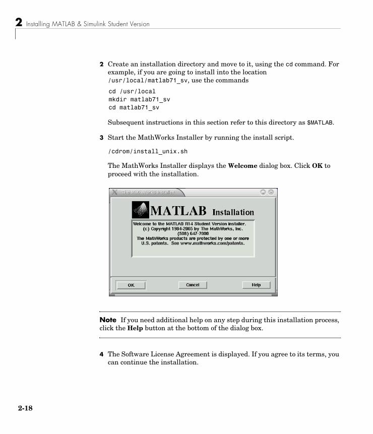
2 Create an installation directory and move to it, using the cd command. For example, if you are going to install into the location /usr/local/matlab71_sv, use the commands
cd /usr/localmkdir matlab71_svcd matlab71_sv
Subsequent instructions in this section refer to this directory as $MATLAB.
3 Start the MathWorks Installer by running the install script.
/cdrom/install_unix.sh
The MathWorks Installer displays the Welcome dialog box. Click OK to proceed with the installation.
Note If you need additional help on any step during this installation process, click the Help button at the bottom of the dialog box.
4 The Software License Agreement is displayed. If you agree to its terms, you can continue the installation.
8
Installing on Linux
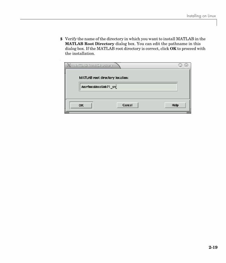
5 Verify the name of the directory in which you want to install MATLAB in the MATLAB Root Directory dialog box. You can edit the pathname in this dialog box. If the MATLAB root directory is correct, click OK to proceed with the installation.
.
2-19
2 Installing MATLAB & Simulink Student Version
2-2
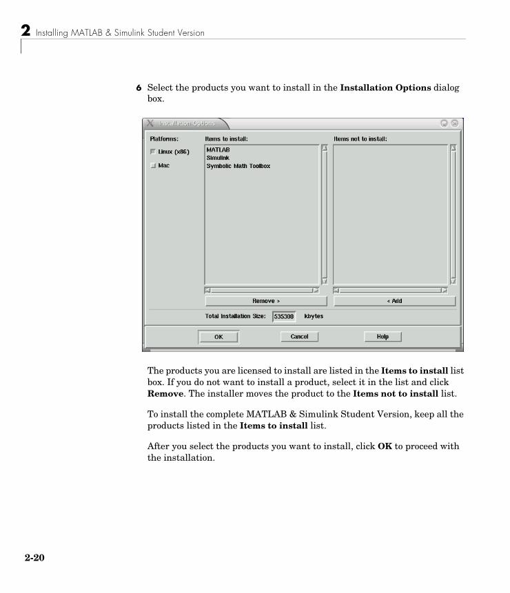
6 Select the products you want to install in the Installation Options dialog box.
The products you are licensed to install are listed in the Items to install list box. If you do not want to install a product, select it in the list and click Remove. The installer moves the product to the Items not to install list.
To install the complete MATLAB & Simulink Student Version, keep all the products listed in the Items to install list.
After you select the products you want to install, click OK to proceed with the installation.
0
Installing on Linux
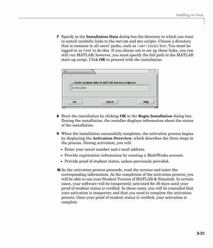
7 Specify in the Installation Data dialog box the directory in which you want to install symbolic links to the matlab and mex scripts. Choose a directory that is common to all users’ paths, such as /usr/local/bin. You must be logged in as root to do this. If you choose not to set up these links, you can still run MATLAB; however, you must specify the full path to the MATLAB start-up script. Click OK to proceed with the installation.
8 Start the installation by clicking OK in the Begin Installation dialog box. During the installation, the installer displays information about the status of the installation.
9 When the installation successfully completes, the activation process begins by displaying the Activation Overview, which describes the three steps in the process. During activation, you will:
- Enter your serial number and e-mail address.
- Provide registration information by creating a MathWorks account.
- Provide proof of student status, unless previously provided.
10 As the activation process proceeds, read the screens and enter the corresponding information. At the completion of the activation process, you will be able to use your Student Version of MATLAB & Simulink. In certain cases, your software will be temporarily activated for 30 days until your proof of student status is verified. In these cases, you will be reminded that your activation is temporary and that you need to complete the activation process. Once your proof of student status is verified, your activation is complete.
2-21
2 Installing MATLAB & Simulink Student Version
2-2
Note If you encounter a problem during the activation process, check www.mathworks.com/academia/student_version/activation.html for more information.
11 To start MATLAB, enter the matlab command. If you did not set up symbolic links in a directory on your path, you must provide the full pathname to the matlab command
$MATLAB/bin/matlab
where $MATLAB represents your MATLAB installation directory.
Installing Additional ToolboxesTo purchase additional toolboxes, visit the MathWorks Store at www.mathworks.com/store. Once you purchase a toolbox, the product and its online documentation are downloaded to your computer. When you download a toolbox on Linux, you receive a tar file (a standard, compressed archive format).
To install the toolbox and documentation, you must
1 Place the tar file in your installation directory ($MATLAB) and extract the files from the archive. Use the following syntax.
tar -xf filename
2 Start the MathWorks Installer.
install
After you successfully install the toolbox and documentation, all of its functionality will be available to you when you start MATLAB.
Accessing the Online Documentation (Help)To access the online documentation (Help), select Full Product Family Help from the Help menu in the MATLAB desktop. You can also type helpbrowser at the MATLAB prompt.
2
3
Introduction
This chapter introduces MATLAB and Simulink, the documentation set, how to start and stop MATLAB, and the MATLAB desktop.
About MATLAB and Simulink (p. 3-2) Overview of the products
MATLAB Documentation (p. 3-5) Overview of the documentation set
Starting and Quitting MATLAB (p. 3-7)
Steps to run and exit MATLAB
3 Introduction
3-2
About MATLAB and Simulink
What Is MATLAB? MATLAB is a high-performance language for technical computing. It integrates computation, visualization, and programming in an easy-to-use environment where problems and solutions are expressed in familiar mathematical notation. Typical uses include
• Math and computation
• Algorithm development
• Data acquisition
• Modeling, simulation, and prototyping
• Data analysis, exploration, and visualization
• Scientific and engineering graphics
• Application development, including graphical user interface building
MATLAB is an interactive system whose basic data element is an array that does not require dimensioning. This allows you to solve many technical computing problems, especially those with matrix and vector formulations, in a fraction of the time it would take to write a program in a scalar noninteractive language such as C or Fortran.
The name MATLAB stands for matrix laboratory. MATLAB was originally written to provide easy access to matrix software developed by the LINPACK and EISPACK projects. Today, MATLAB engines incorporate the LAPACK and BLAS libraries, embedding the state of the art in software for matrix computation.
MATLAB has evolved over a period of years with input from many users. In university environments, it is the standard instructional tool for introductory and advanced courses in mathematics, engineering, and science. In industry, MATLAB is the tool of choice for high-productivity research, development, and analysis.
ToolboxesMATLAB features a family of add-on application-specific solutions called toolboxes. Very important to most users of MATLAB, toolboxes allow you to learn and apply specialized technology. Toolboxes are comprehensive
About MATLAB and Simulink
collections of MATLAB functions (M-files) that extend the MATLAB environment to solve particular classes of problems. Areas in which toolboxes are available include signal processing, control systems, neural networks, fuzzy logic, wavelets, simulation, and many others.
The MATLAB SystemThe MATLAB system consists of five main parts:
Development Environment. This is the set of tools and facilities that help you use MATLAB functions and files. Many of these tools are graphical user interfaces. It includes the MATLAB desktop and Command Window, a command history, an editor and debugger, and browsers for viewing help, the workspace, files, and the search path.
The MATLAB Mathematical Function Library. This is a vast collection of computational algorithms ranging from elementary functions, like sum, sine, cosine, and complex arithmetic, to more sophisticated functions like matrix inverse, matrix eigenvalues, Bessel functions, and fast Fourier transforms.
The MATLAB Language. This is a high-level matrix/array language with control flow statements, functions, data structures, input/output, and object-oriented programming features. It allows both “programming in the small” to rapidly create quick and dirty throw-away programs, and “programming in the large” to create large and complex application programs.
Graphics. MATLAB has extensive facilities for displaying vectors and matrices as graphs, as well as annotating and printing these graphs. It includes high-level functions for two-dimensional and three-dimensional data visualization, image processing, animation, and presentation graphics. It also includes low-level functions that allow you to fully customize the appearance of graphics as well as to build complete graphical user interfaces on your MATLAB applications.
The MATLAB Application Program Interface (API). This is a library that allows you to write C and Fortran programs that interact with MATLAB. It includes facilities for calling routines from MATLAB (dynamic linking), calling MATLAB as a computational engine, and for reading and writing MAT-files.
3-3
3 Introduction
3-4
What Is Simulink?Simulink is an interactive environment for modeling, simulating, and analyzing dynamic, multidomain systems. It lets you build a block diagram, simulate the system’s behavior, evaluate its performance, and refine the design. Simulink integrates seamlessly with MATLAB, providing you with immediate access to an extensive range of analysis and design tools. These benefits make Simulink the tool of choice for control system design, DSP design, communications system design, and other simulation applications.
Blocksets are collections of application-specific blocks that support multiple design areas, including electrical power-system modeling, digital signal processing, fixed-point algorithm development, and more. These blocks can be incorporated directly into your Simulink models.
Real-Time Workshop® is a program that generates optimized, portable, and customizable ANSI C code from Simulink models. Generated code can run on PC hardware, DSPs, microcontrollers on bare-board environments, and with commercial or proprietary real-time operating systems.
What Is Stateflow?Stateflow is an interactive design tool for modeling and simulating complex reactive systems. Tightly integrated with Simulink and MATLAB, Stateflow provides Simulink users with an elegant solution for designing embedded systems by giving them an efficient way to incorporate complex control and supervisory logic within their Simulink models.
With Stateflow, you can quickly develop graphical models of event-driven systems using finite state machine theory, statechart formalisms, and flow diagram notation. Together, Stateflow and Simulink serve as an executable specification and virtual prototype of your system design.
Note Your MATLAB & Simulink Student Version includes a demo version of Stateflow.
MATLAB Documentation
MATLAB DocumentationMATLAB provides extensive documentation, in both printed and online format, to help you learn about and use all of its features. If you are a new user, start with the MATLAB specific sections in this book. It covers all the primary MATLAB features at a high level, including many examples.
The MATLAB online help provides task-oriented and reference information about MATLAB features. MATLAB documentation is also available in printed form and in PDF format.
MATLAB Online HelpTo view the online documentation, select MATLAB Help from the Help menu in MATLAB. The MATLAB documentation is organized into these main topics:
• Desktop Tools and Development Environment — Startup and shutdown, the desktop, and other tools that help you use MATLAB
• Mathematics — Mathematical operations and data analysis
• Programming — The MATLAB language and how to develop MATLAB applications
• Graphics — Tools and techniques for plotting, graph annotation, printing, and programming with Handle Graphics®
• 3-D Visualization — Visualizing surface and volume data, transparency, and viewing and lighting techniques
• Creating Graphical User Interfaces — GUI-building tools and how to write callback functions
• External Interfaces — MEX-files, the MATLAB engine, and interfacing to Java, COM, and the serial port
MATLAB also includes reference documentation for all MATLAB functions:
• Functions — Categorical List — Lists all MATLAB functions grouped into categories
• Handle Graphics Property Browser — Provides easy access to descriptions of graphics object properties
• External Interfaces Reference — Covers those functions used by the MATLAB external interfaces, providing information on syntax in the calling language, description, arguments, return values, and examples
3-5
3 Introduction
3-6
The MATLAB online documentation also includes
• Examples — An index of examples included in the documentation
• Release Notes — New features and known problems in the current release
• Printable Documentation — PDF versions of the documentation suitable for printing
For more information about using the Help browser, see Chapter 8, “Desktop Tools and Development Environment.”
Note References to UNIX in the documentation include both Linux and Mac OS X.
Starting and Quitting MATLAB
Starting and Quitting MATLAB
Starting MATLABOn Windows platforms, start MATLAB by double-clicking the MATLAB shortcut icon on your Windows desktop.
On Mac OS X platforms, start MATLAB by double-clicking the MATLAB icon on your desktop.
On Linux platforms, start MATLAB by typing matlab at the operating system prompt.
You can customize MATLAB startup. For example, you can change the directory in which MATLAB starts or automatically execute MATLAB statements in a script file named startup.m.
For More Information See “Starting MATLAB” in the Desktop Tools and Development Environment documentation.
Quitting MATLABTo end your MATLAB session, select File -> Exit MATLAB in the desktop, or type quit in the Command Window. You can run a script file named finish.m each time MATLAB quits that, for example, executes functions to save the workspace, or displays a quit confirmation dialog box.
For More Information See “Quitting MATLAB” in the Desktop Tools and Development Environment documentation.
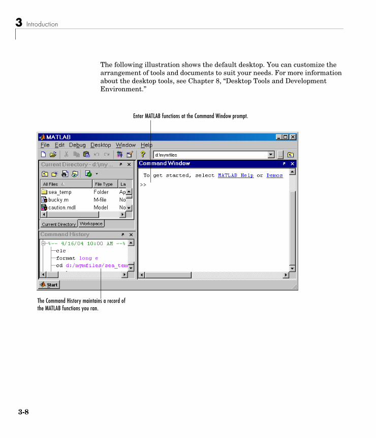
MATLAB DesktopWhen you start MATLAB, the MATLAB desktop appears, containing tools (graphical user interfaces) for managing files, variables, and applications associated with MATLAB.
3-7
3 Introduction
3-8
The following illustration shows the default desktop. You can customize the arrangement of tools and documents to suit your needs. For more information about the desktop tools, see Chapter 8, “Desktop Tools and Development Environment.”
Enter MATLAB functions at the Command Window prompt.
The Command History maintains a record of the MATLAB functions you ran.
4
Matrices and Arrays
This chapter introduces you to MATLAB by teaching you how to handle matrices.
Matrices and Magic Squares (p. 4-2) Enter matrices, perform matrix operations, and access matrix elements.
Expressions (p. 4-10) Work with variables, numbers, operators, functions, and expressions.
Working with Matrices (p. 4-14) Generate matrices, load matrices, create matrices from M-files and concatenation, and delete matrix rows and columns.
More About Matrices and Arrays (p. 4-18)
Use matrices for linear algebra, work with arrays, multivariate data, scalar expansion, and logical subscripting, and use the find function.
Controlling Command Window Input and Output (p. 4-28)
Change output format, suppress output, enter long lines, and edit at the command line.
4 Matrices and Arrays
4-2
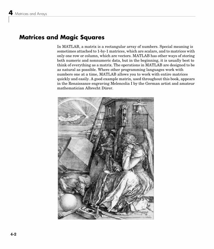
Matrices and Magic SquaresIn MATLAB, a matrix is a rectangular array of numbers. Special meaning is sometimes attached to 1-by-1 matrices, which are scalars, and to matrices with only one row or column, which are vectors. MATLAB has other ways of storing both numeric and nonnumeric data, but in the beginning, it is usually best to think of everything as a matrix. The operations in MATLAB are designed to be as natural as possible. Where other programming languages work with numbers one at a time, MATLAB allows you to work with entire matrices quickly and easily. A good example matrix, used throughout this book, appears in the Renaissance engraving Melencolia I by the German artist and amateur mathematician Albrecht Dürer.
Matrices and Magic Squares
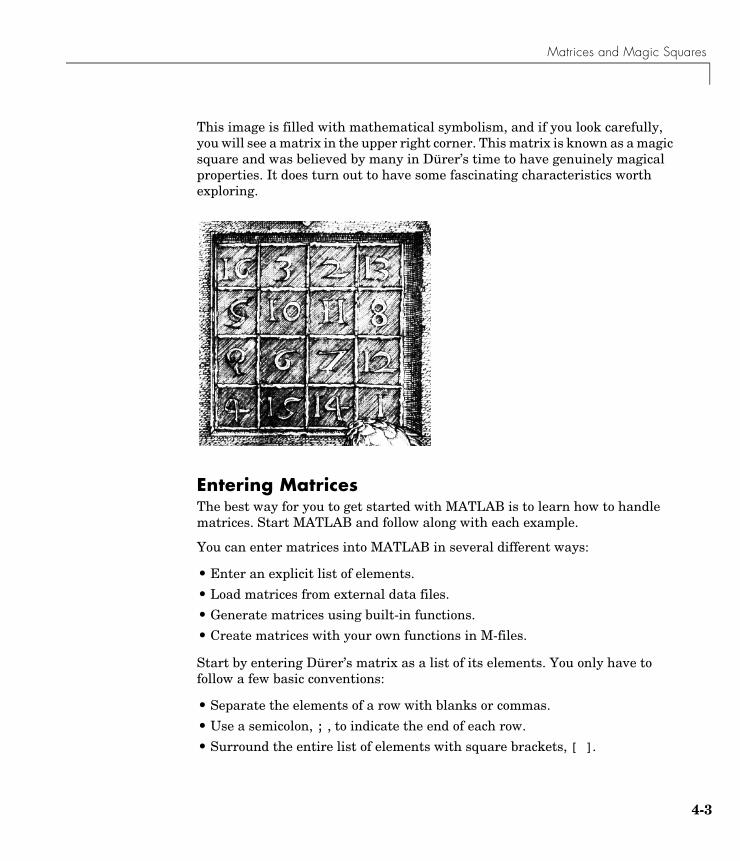
This image is filled with mathematical symbolism, and if you look carefully, you will see a matrix in the upper right corner. This matrix is known as a magic square and was believed by many in Dürer’s time to have genuinely magical properties. It does turn out to have some fascinating characteristics worth exploring.
Entering MatricesThe best way for you to get started with MATLAB is to learn how to handle matrices. Start MATLAB and follow along with each example.
You can enter matrices into MATLAB in several different ways:
• Enter an explicit list of elements.
• Load matrices from external data files.
• Generate matrices using built-in functions.
• Create matrices with your own functions in M-files.
Start by entering Dürer’s matrix as a list of its elements. You only have to follow a few basic conventions:
• Separate the elements of a row with blanks or commas.
• Use a semicolon, ; , to indicate the end of each row.
• Surround the entire list of elements with square brackets, [ ].
4-3
4 Matrices and Arrays
4-4
To enter Dürer’s matrix, simply type in the Command Window
A = [16 3 2 13; 5 10 11 8; 9 6 7 12; 4 15 14 1]
MATLAB displays the matrix you just entered.
A = 16 3 2 13 5 10 11 8 9 6 7 12 4 15 14 1
This matrix matches the numbers in the engraving. Once you have entered the matrix, it is automatically remembered in the MATLAB workspace. You can refer to it simply as A. Now that you have A in the workspace, take a look at what makes it so interesting. Why is it magic?
sum, transpose, and diagYou are probably already aware that the special properties of a magic square have to do with the various ways of summing its elements. If you take the sum along any row or column, or along either of the two main diagonals, you will always get the same number. Let us verify that using MATLAB. The first statement to try is
sum(A)
MATLAB replies with
ans = 34 34 34 34
When you do not specify an output variable, MATLAB uses the variable ans, short for answer, to store the results of a calculation. You have computed a row vector containing the sums of the columns of A. Sure enough, each of the columns has the same sum, the magic sum, 34.
How about the row sums? MATLAB has a preference for working with the columns of a matrix, so the easiest way to get the row sums is to transpose the matrix, compute the column sums of the transpose, and then transpose the result.
MATLAB has two transpose operators. The apostrophe operator (e.g., A') performs a complex conjugate transposition. It flips a matrix about its main
Matrices and Magic Squares
diagonal, and also changes the sign of the imaginary component of any complex elements of the matrix. The apostrophe-dot operator (e.g., A'.), transposes without affecting the sign of complex elements. For matrices containing all real elements, the two operators return the same result.
So
A'produces
ans = 16 5 9 4 3 10 6 15 2 11 7 14 13 8 12 1
and
sum(A')'
produces a column vector containing the row sums
ans = 34 34 34 34
The sum of the elements on the main diagonal is obtained with the sum and the diag functions.
diag(A)
produces
ans = 16 10 7 1
and
sum(diag(A))
produces
4-5
4 Matrices and Arrays
4-6
ans = 34
The other diagonal, the so-called antidiagonal, is not so important mathematically, so MATLAB does not have a ready-made function for it. But a function originally intended for use in graphics, fliplr, flips a matrix from left to right.
sum(diag(fliplr(A)))
ans = 34
You have verified that the matrix in Dürer’s engraving is indeed a magic square and, in the process, have sampled a few MATLAB matrix operations. The following sections continue to use this matrix to illustrate additional MATLAB capabilities.
SubscriptsThe element in row i and column j of A is denoted by A(i,j). For example, A(4,2) is the number in the fourth row and second column. For our magic square, A(4,2) is 15. So to compute the sum of the elements in the fourth column of A, type
A(1,4) + A(2,4) + A(3,4) + A(4,4)
This produces
ans = 34
but is not the most elegant way of summing a single column.
It is also possible to refer to the elements of a matrix with a single subscript, A(k). This is the usual way of referencing row and column vectors. But it can also apply to a fully two-dimensional matrix, in which case the array is regarded as one long column vector formed from the columns of the original matrix. So, for our magic square, A(8) is another way of referring to the value 15 stored in A(4,2).
If you try to use the value of an element outside of the matrix, it is an error.
t = A(4,5)
Matrices and Magic Squares
Index exceeds matrix dimensions.
On the other hand, if you store a value in an element outside of the matrix, the size increases to accommodate the newcomer.
X = A;X(4,5) = 17
X = 16 3 2 13 0 5 10 11 8 0 9 6 7 12 0 4 15 14 1 17
The Colon OperatorThe colon, :, is one of the most important MATLAB operators. It occurs in several different forms. The expression
1:10
is a row vector containing the integers from 1 to 10,
1 2 3 4 5 6 7 8 9 10
To obtain nonunit spacing, specify an increment. For example,
100:-7:50
is
100 93 86 79 72 65 58 51
and
0:pi/4:pi
is
0 0.7854 1.5708 2.3562 3.1416
Subscript expressions involving colons refer to portions of a matrix.
A(1:k,j)
is the first k elements of the jth column of A. So
4-7
4 Matrices and Arrays
4-8
sum(A(1:4,4))
computes the sum of the fourth column. But there is a better way. The colon by itself refers to all the elements in a row or column of a matrix and the keyword end refers to the last row or column. So
sum(A(:,end))
computes the sum of the elements in the last column of A.
ans = 34
Why is the magic sum for a 4-by-4 square equal to 34? If the integers from 1 to 16 are sorted into four groups with equal sums, that sum must be
sum(1:16)/4
which, of course, is
ans = 34
The magic FunctionMATLAB actually has a built-in function that creates magic squares of almost any size. Not surprisingly, this function is named magic.
B = magic(4)
B = 16 2 3 13 5 11 10 8 9 7 6 12 4 14 15 1
This matrix is almost the same as the one in the Dürer engraving and has all the same “magic” properties; the only difference is that the two middle columns are exchanged.
To make this B into Dürer’s A, swap the two middle columns.
A = B(:,[1 3 2 4])
Matrices and Magic Squares
This says, for each of the rows of matrix B, reorder the elements in the order 1, 3, 2, 4. It produces
A = 16 3 2 13 5 10 11 8 9 6 7 12 4 15 14 1
Why would Dürer go to the trouble of rearranging the columns when he could have used MATLAB ordering? No doubt he wanted to include the date of the engraving, 1514, at the bottom of his magic square.
4-9
4 Matrices and Arrays
4-1
ExpressionsLike most other programming languages, MATLAB provides mathematical expressions, but unlike most programming languages, these expressions involve entire matrices. The building blocks of expressions are
• “Variables” on page 4-10
• “Numbers” on page 4-11
• “Operators” on page 4-11
• “Functions” on page 4-12
See also “Examples of Expressions” on page 4-13.
VariablesMATLAB does not require any type declarations or dimension statements. When MATLAB encounters a new variable name, it automatically creates the variable and allocates the appropriate amount of storage. If the variable already exists, MATLAB changes its contents and, if necessary, allocates new storage. For example,
num_students = 25
creates a 1-by-1 matrix named num_students and stores the value 25 in its single element. To view the matrix assigned to any variable, simply enter the variable name.
Variable names consist of a letter, followed by any number of letters, digits, or underscores. MATLAB is case sensitive; it distinguishes between uppercase and lowercase letters. A and a are not the same variable.
Although variable names can be of any length, MATLAB uses only the first N characters of the name, (where N is the number returned by the function namelengthmax), and ignores the rest. Hence, it is important to make each variable name unique in the first N characters to enable MATLAB to distinguish variables.
N = namelengthmaxN = 63
0
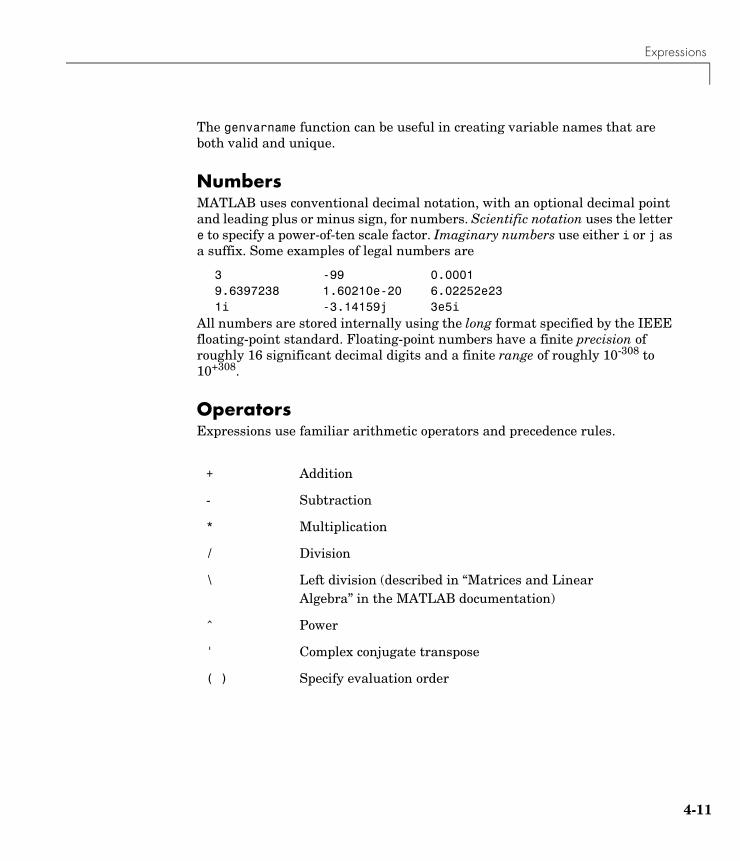
Expressions
The genvarname function can be useful in creating variable names that are both valid and unique.
NumbersMATLAB uses conventional decimal notation, with an optional decimal point and leading plus or minus sign, for numbers. Scientific notation uses the letter e to specify a power-of-ten scale factor. Imaginary numbers use either i or j as a suffix. Some examples of legal numbers are
3 -99 0.00019.6397238 1.60210e-20 6.02252e231i -3.14159j 3e5i
All numbers are stored internally using the long format specified by the IEEE floating-point standard. Floating-point numbers have a finite precision of roughly 16 significant decimal digits and a finite range of roughly 10-308 to 10+308.
Operators Expressions use familiar arithmetic operators and precedence rules.
+ Addition
- Subtraction
* Multiplication
/ Division
\ Left division (described in “Matrices and Linear Algebra” in the MATLAB documentation)
^ Power
' Complex conjugate transpose
( ) Specify evaluation order
4-11
4 Matrices and Arrays
4-1
FunctionsMATLAB provides a large number of standard elementary mathematical functions, including abs, sqrt, exp, and sin. Taking the square root or logarithm of a negative number is not an error; the appropriate complex result is produced automatically. MATLAB also provides many more advanced mathematical functions, including Bessel and gamma functions. Most of these functions accept complex arguments. For a list of the elementary mathematical functions, type
help elfun
For a list of more advanced mathematical and matrix functions, type
help specfunhelp elmat
Some of the functions, like sqrt and sin, are built in. Built-in functions are part of the MATLAB core so they are very efficient, but the computational details are not readily accessible. Other functions, like gamma and sinh, are implemented in M-files.
There are some differences between built-in functions and other functions. For example, for built-in functions, you cannot see the code. For other functions, you can see the code and even modify it if you want.
Several special functions provide values of useful constants.
pi 3.14159265…
i Imaginary unit,
j Same as i
eps Floating-point relative precision,
realmin Smallest floating-point number,
realmax Largest floating-point number,
Inf Infinity
NaN Not-a-number
1–
ε 2 52–=
2 1022–
2 ε–( )21023
2
Expressions
Infinity is generated by dividing a nonzero value by zero, or by evaluating well defined mathematical expressions that overflow, i.e., exceed realmax. Not-a-number is generated by trying to evaluate expressions like 0/0 or Inf-Inf that do not have well defined mathematical values.
The function names are not reserved. It is possible to overwrite any of them with a new variable, such as
eps = 1.e-6
and then use that value in subsequent calculations. The original function can be restored with
clear eps
Examples of ExpressionsYou have already seen several examples of MATLAB expressions. Here are a few more examples, and the resulting values.
rho = (1+sqrt(5))/2rho = 1.6180
a = abs(3+4i)a = 5
z = sqrt(besselk(4/3,rho-i))z = 0.3730+ 0.3214i
huge = exp(log(realmax))huge = 1.7977e+308
toobig = pi*hugetoobig = Inf
4-13
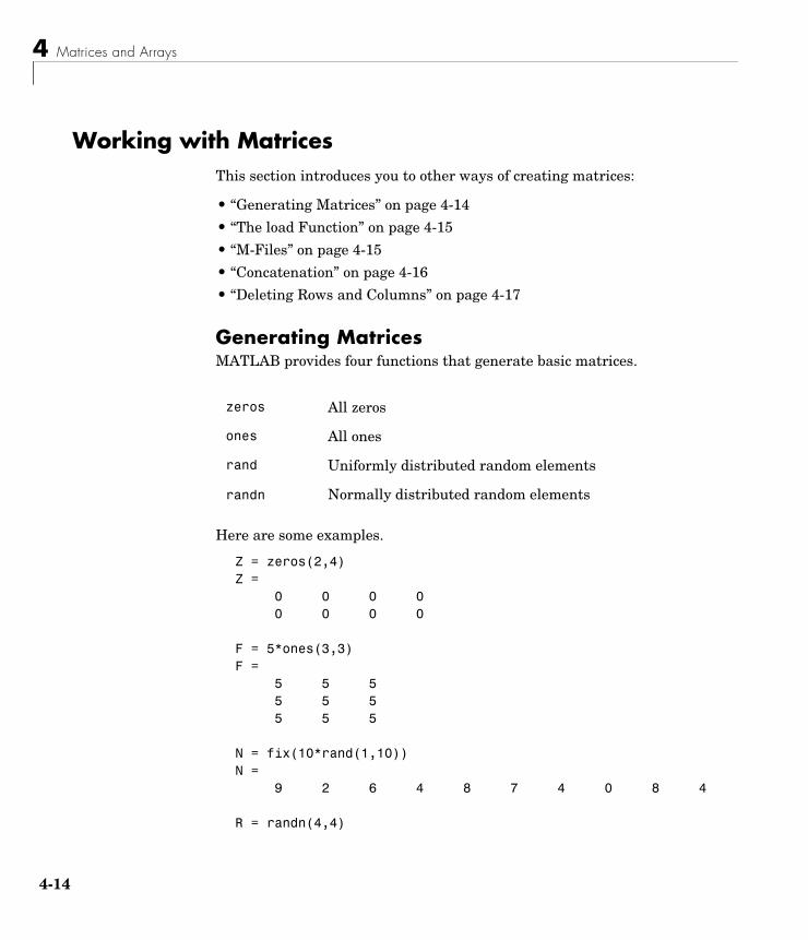
4 Matrices and Arrays
4-1
Working with MatricesThis section introduces you to other ways of creating matrices:
• “Generating Matrices” on page 4-14
• “The load Function” on page 4-15
• “M-Files” on page 4-15
• “Concatenation” on page 4-16
• “Deleting Rows and Columns” on page 4-17
Generating MatricesMATLAB provides four functions that generate basic matrices.
Here are some examples.
Z = zeros(2,4)Z = 0 0 0 0 0 0 0 0
F = 5*ones(3,3)F = 5 5 5 5 5 5 5 5 5
N = fix(10*rand(1,10))N =
9 2 6 4 8 7 4 0 8 4
R = randn(4,4)
zeros All zeros
ones All ones
rand Uniformly distributed random elements
randn Normally distributed random elements
4
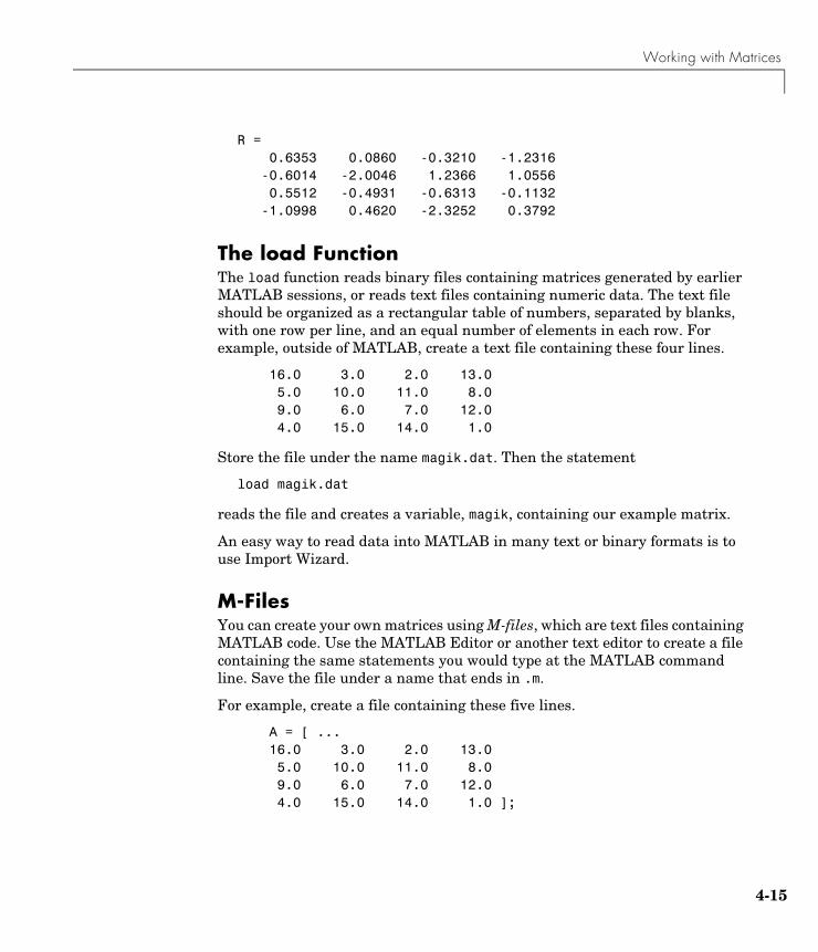
Working with Matrices
R =0.6353 0.0860 -0.3210 -1.2316
-0.6014 -2.0046 1.2366 1.0556 0.5512 -0.4931 -0.6313 -0.1132 -1.0998 0.4620 -2.3252 0.3792
The load FunctionThe load function reads binary files containing matrices generated by earlier MATLAB sessions, or reads text files containing numeric data. The text file should be organized as a rectangular table of numbers, separated by blanks, with one row per line, and an equal number of elements in each row. For example, outside of MATLAB, create a text file containing these four lines.
16.0 3.0 2.0 13.0 5.0 10.0 11.0 8.0 9.0 6.0 7.0 12.0 4.0 15.0 14.0 1.0
Store the file under the name magik.dat. Then the statement
load magik.dat
reads the file and creates a variable, magik, containing our example matrix.
An easy way to read data into MATLAB in many text or binary formats is to use Import Wizard.
M-FilesYou can create your own matrices using M-files, which are text files containing MATLAB code. Use the MATLAB Editor or another text editor to create a file containing the same statements you would type at the MATLAB command line. Save the file under a name that ends in .m.
For example, create a file containing these five lines.
A = [ ... 16.0 3.0 2.0 13.0 5.0 10.0 11.0 8.0 9.0 6.0 7.0 12.0 4.0 15.0 14.0 1.0 ];
4-15
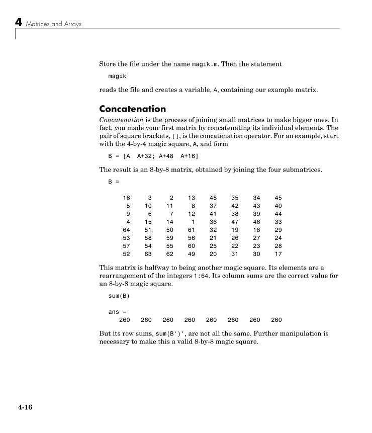
4 Matrices and Arrays
4-1
Store the file under the name magik.m. Then the statement
magik
reads the file and creates a variable, A, containing our example matrix.
ConcatenationConcatenation is the process of joining small matrices to make bigger ones. In fact, you made your first matrix by concatenating its individual elements. The pair of square brackets, [], is the concatenation operator. For an example, start with the 4-by-4 magic square, A, and form
B = [A A+32; A+48 A+16]
The result is an 8-by-8 matrix, obtained by joining the four submatrices.
B =
16 3 2 13 48 35 34 45 5 10 11 8 37 42 43 40 9 6 7 12 41 38 39 44 4 15 14 1 36 47 46 33 64 51 50 61 32 19 18 29 53 58 59 56 21 26 27 24 57 54 55 60 25 22 23 28 52 63 62 49 20 31 30 17
This matrix is halfway to being another magic square. Its elements are a rearrangement of the integers 1:64. Its column sums are the correct value for an 8-by-8 magic square.
sum(B)
ans = 260 260 260 260 260 260 260 260
But its row sums, sum(B')', are not all the same. Further manipulation is necessary to make this a valid 8-by-8 magic square.
6
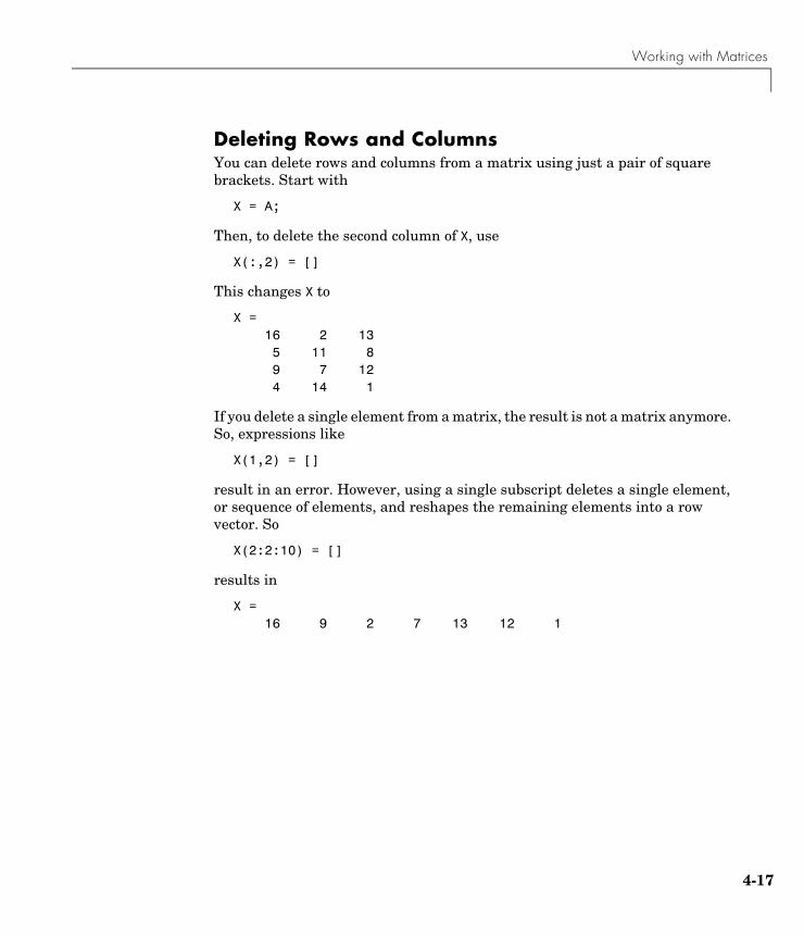
Working with Matrices
Deleting Rows and ColumnsYou can delete rows and columns from a matrix using just a pair of square brackets. Start with
X = A;
Then, to delete the second column of X, use
X(:,2) = []
This changes X to
X = 16 2 13 5 11 8 9 7 12 4 14 1
If you delete a single element from a matrix, the result is not a matrix anymore. So, expressions like
X(1,2) = []
result in an error. However, using a single subscript deletes a single element, or sequence of elements, and reshapes the remaining elements into a row vector. So
X(2:2:10) = []
results in
X = 16 9 2 7 13 12 1
4-17
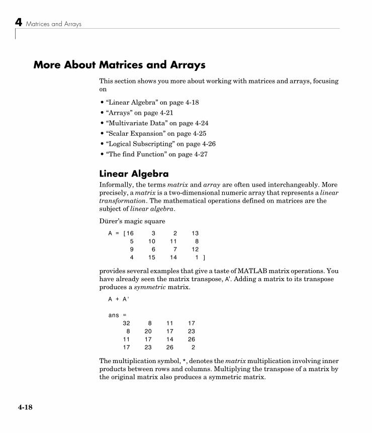
4 Matrices and Arrays
4-1
More About Matrices and ArraysThis section shows you more about working with matrices and arrays, focusing on
• “Linear Algebra” on page 4-18
• “Arrays” on page 4-21
• “Multivariate Data” on page 4-24
• “Scalar Expansion” on page 4-25
• “Logical Subscripting” on page 4-26
• “The find Function” on page 4-27
Linear AlgebraInformally, the terms matrix and array are often used interchangeably. More precisely, a matrix is a two-dimensional numeric array that represents a linear transformation. The mathematical operations defined on matrices are the subject of linear algebra.
Dürer’s magic square
A = [16 3 2 13 5 10 11 8 9 6 7 12 4 15 14 1 ]
provides several examples that give a taste of MATLAB matrix operations. You have already seen the matrix transpose, A'. Adding a matrix to its transpose produces a symmetric matrix.
A + A'
ans = 32 8 11 17 8 20 17 23 11 17 14 26 17 23 26 2
The multiplication symbol, *, denotes the matrix multiplication involving inner products between rows and columns. Multiplying the transpose of a matrix by the original matrix also produces a symmetric matrix.
8
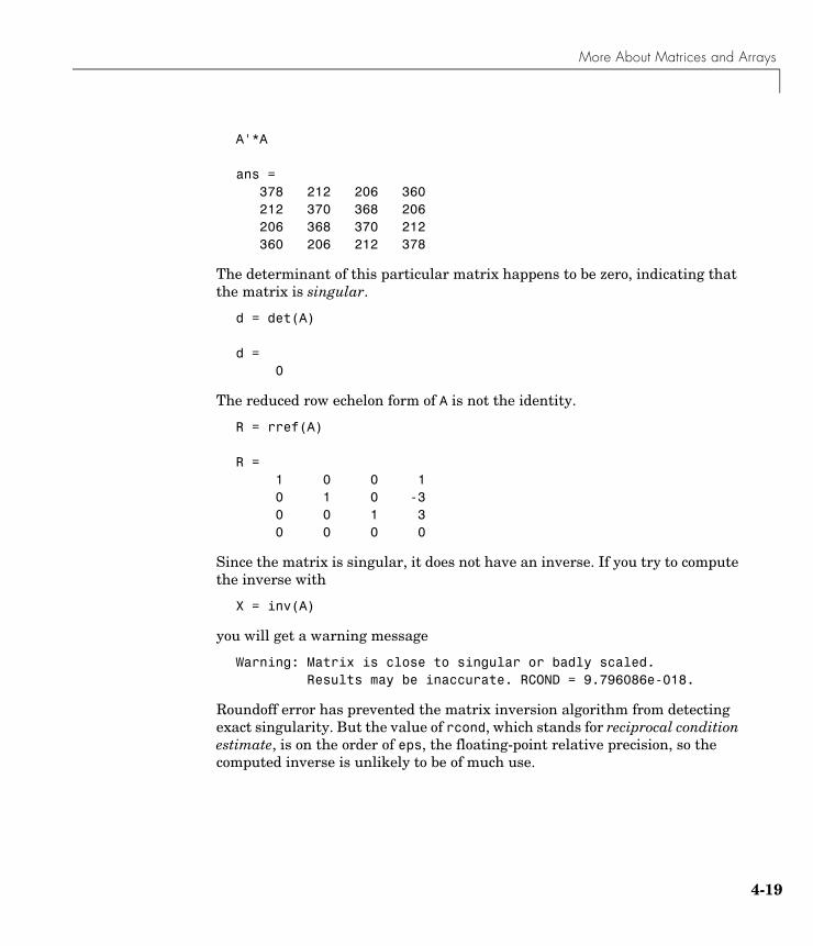
More About Matrices and Arrays
A'*A
ans = 378 212 206 360 212 370 368 206 206 368 370 212 360 206 212 378
The determinant of this particular matrix happens to be zero, indicating that the matrix is singular.
d = det(A)
d = 0
The reduced row echelon form of A is not the identity.
R = rref(A)
R = 1 0 0 1 0 1 0 -3 0 0 1 3 0 0 0 0
Since the matrix is singular, it does not have an inverse. If you try to compute the inverse with
X = inv(A)
you will get a warning message
Warning: Matrix is close to singular or badly scaled. Results may be inaccurate. RCOND = 9.796086e-018.
Roundoff error has prevented the matrix inversion algorithm from detecting exact singularity. But the value of rcond, which stands for reciprocal condition estimate, is on the order of eps, the floating-point relative precision, so the computed inverse is unlikely to be of much use.
4-19
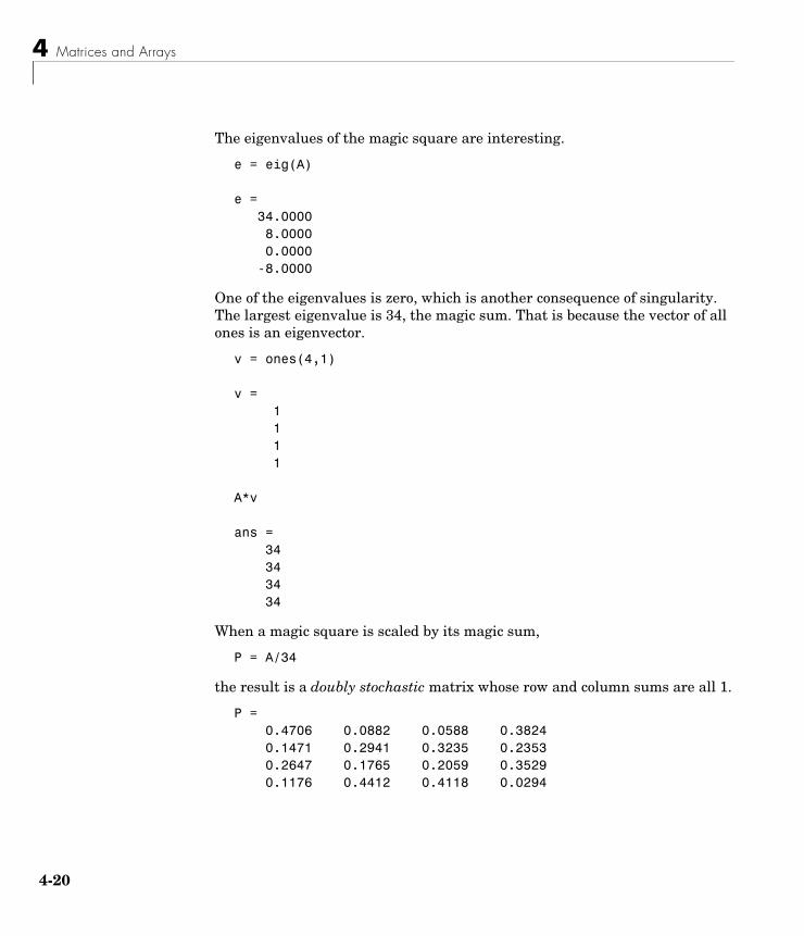
4 Matrices and Arrays
4-2
The eigenvalues of the magic square are interesting.
e = eig(A)
e = 34.0000 8.0000 0.0000 -8.0000
One of the eigenvalues is zero, which is another consequence of singularity. The largest eigenvalue is 34, the magic sum. That is because the vector of all ones is an eigenvector.
v = ones(4,1)
v = 1 1 1 1
A*v
ans = 34 34 34 34
When a magic square is scaled by its magic sum,
P = A/34
the result is a doubly stochastic matrix whose row and column sums are all 1.
P = 0.4706 0.0882 0.0588 0.3824 0.1471 0.2941 0.3235 0.2353 0.2647 0.1765 0.2059 0.3529 0.1176 0.4412 0.4118 0.0294
0
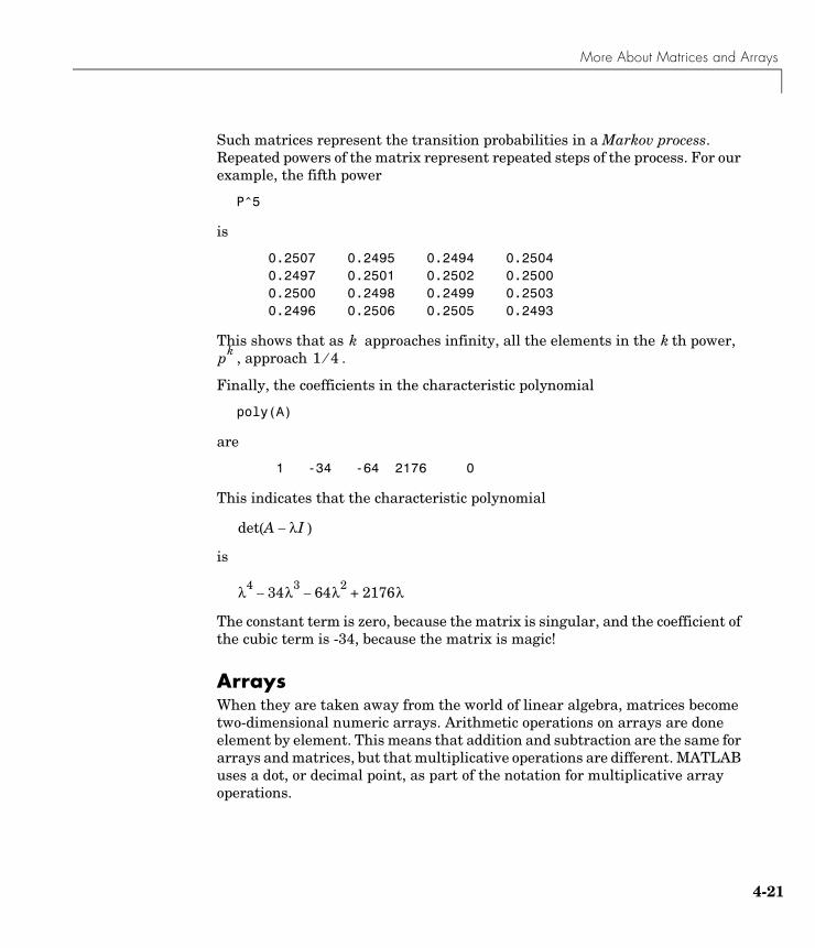
More About Matrices and Arrays
Such matrices represent the transition probabilities in a Markov process. Repeated powers of the matrix represent repeated steps of the process. For our example, the fifth power
P^5
is
0.2507 0.2495 0.2494 0.2504 0.2497 0.2501 0.2502 0.2500 0.2500 0.2498 0.2499 0.2503 0.2496 0.2506 0.2505 0.2493
This shows that as approaches infinity, all the elements in the th power, , approach .
Finally, the coefficients in the characteristic polynomial
poly(A)
are
1 -34 -64 2176 0
This indicates that the characteristic polynomial
is
The constant term is zero, because the matrix is singular, and the coefficient of the cubic term is -34, because the matrix is magic!
ArraysWhen they are taken away from the world of linear algebra, matrices become two-dimensional numeric arrays. Arithmetic operations on arrays are done element by element. This means that addition and subtraction are the same for arrays and matrices, but that multiplicative operations are different. MATLAB uses a dot, or decimal point, as part of the notation for multiplicative array operations.
k kpk 1 4⁄
det A λI–( )
λ4 34λ3– 64λ2
– 2176λ+
4-21
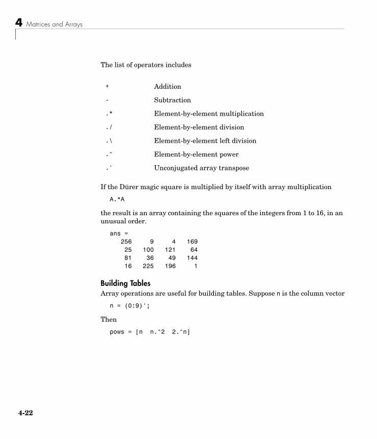
4 Matrices and Arrays
4-2
The list of operators includes
If the Dürer magic square is multiplied by itself with array multiplication
A.*A
the result is an array containing the squares of the integers from 1 to 16, in an unusual order.
ans = 256 9 4 169 25 100 121 64 81 36 49 144 16 225 196 1
Building TablesArray operations are useful for building tables. Suppose n is the column vector
n = (0:9)';
Then
pows = [n n.^2 2.^n]
+ Addition
- Subtraction
.* Element-by-element multiplication
./ Element-by-element division
.\ Element-by-element left division
.^ Element-by-element power
.' Unconjugated array transpose
2
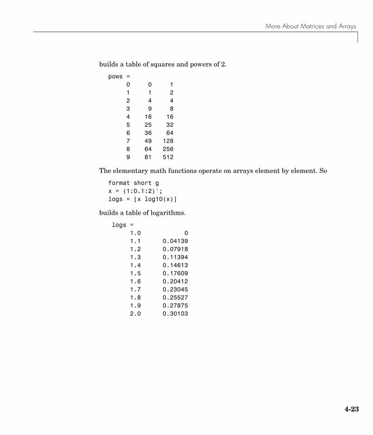
More About Matrices and Arrays
builds a table of squares and powers of 2.
pows = 0 0 1 1 1 2 2 4 4 3 9 8 4 16 16 5 25 32 6 36 64 7 49 128 8 64 256 9 81 512
The elementary math functions operate on arrays element by element. So
format short gx = (1:0.1:2)';logs = [x log10(x)]
builds a table of logarithms.
logs = 1.0 0 1.1 0.04139 1.2 0.07918 1.3 0.11394 1.4 0.14613 1.5 0.17609 1.6 0.20412 1.7 0.23045 1.8 0.25527 1.9 0.27875 2.0 0.30103
4-23
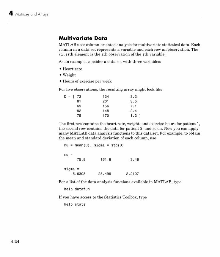
4 Matrices and Arrays
4-2
Multivariate DataMATLAB uses column-oriented analysis for multivariate statistical data. Each column in a data set represents a variable and each row an observation. The (i,j)th element is the ith observation of the jth variable.
As an example, consider a data set with three variables:
• Heart rate
• Weight
• Hours of exercise per week
For five observations, the resulting array might look like
D = [ 72 134 3.2 81 201 3.5 69 156 7.1 82 148 2.4 75 170 1.2 ]
The first row contains the heart rate, weight, and exercise hours for patient 1, the second row contains the data for patient 2, and so on. Now you can apply many MATLAB data analysis functions to this data set. For example, to obtain the mean and standard deviation of each column, use
mu = mean(D), sigma = std(D)
mu =75.8 161.8 3.48
sigma =5.6303 25.499 2.2107
For a list of the data analysis functions available in MATLAB, type
help datafun
If you have access to the Statistics Toolbox, type
help stats
4
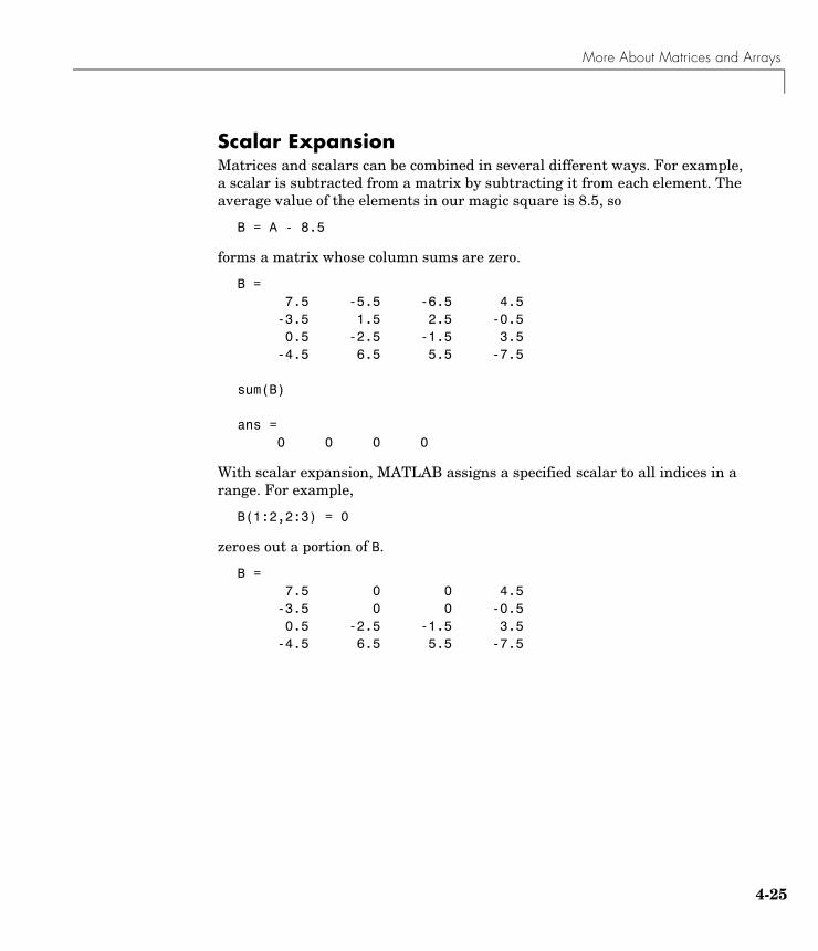
More About Matrices and Arrays
Scalar ExpansionMatrices and scalars can be combined in several different ways. For example, a scalar is subtracted from a matrix by subtracting it from each element. The average value of the elements in our magic square is 8.5, so
B = A - 8.5
forms a matrix whose column sums are zero.
B = 7.5 -5.5 -6.5 4.5 -3.5 1.5 2.5 -0.5 0.5 -2.5 -1.5 3.5 -4.5 6.5 5.5 -7.5
sum(B)
ans = 0 0 0 0
With scalar expansion, MATLAB assigns a specified scalar to all indices in a range. For example,
B(1:2,2:3) = 0
zeroes out a portion of B.
B = 7.5 0 0 4.5 -3.5 0 0 -0.5 0.5 -2.5 -1.5 3.5 -4.5 6.5 5.5 -7.5
4-25
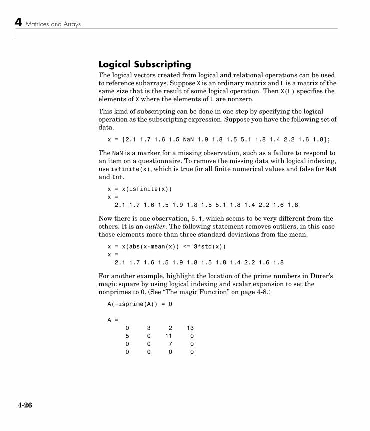
4 Matrices and Arrays
4-2
Logical SubscriptingThe logical vectors created from logical and relational operations can be used to reference subarrays. Suppose X is an ordinary matrix and L is a matrix of the same size that is the result of some logical operation. Then X(L) specifies the elements of X where the elements of L are nonzero.
This kind of subscripting can be done in one step by specifying the logical operation as the subscripting expression. Suppose you have the following set of data.
x = [2.1 1.7 1.6 1.5 NaN 1.9 1.8 1.5 5.1 1.8 1.4 2.2 1.6 1.8];
The NaN is a marker for a missing observation, such as a failure to respond to an item on a questionnaire. To remove the missing data with logical indexing, use isfinite(x), which is true for all finite numerical values and false for NaN and Inf.
x = x(isfinite(x))x = 2.1 1.7 1.6 1.5 1.9 1.8 1.5 5.1 1.8 1.4 2.2 1.6 1.8
Now there is one observation, 5.1, which seems to be very different from the others. It is an outlier. The following statement removes outliers, in this case those elements more than three standard deviations from the mean.
x = x(abs(x-mean(x)) <= 3*std(x))x =2.1 1.7 1.6 1.5 1.9 1.8 1.5 1.8 1.4 2.2 1.6 1.8
For another example, highlight the location of the prime numbers in Dürer’s magic square by using logical indexing and scalar expansion to set the nonprimes to 0. (See “The magic Function” on page 4-8.)
A(~isprime(A)) = 0
A = 0 3 2 13 5 0 11 0 0 0 7 0 0 0 0 0
6
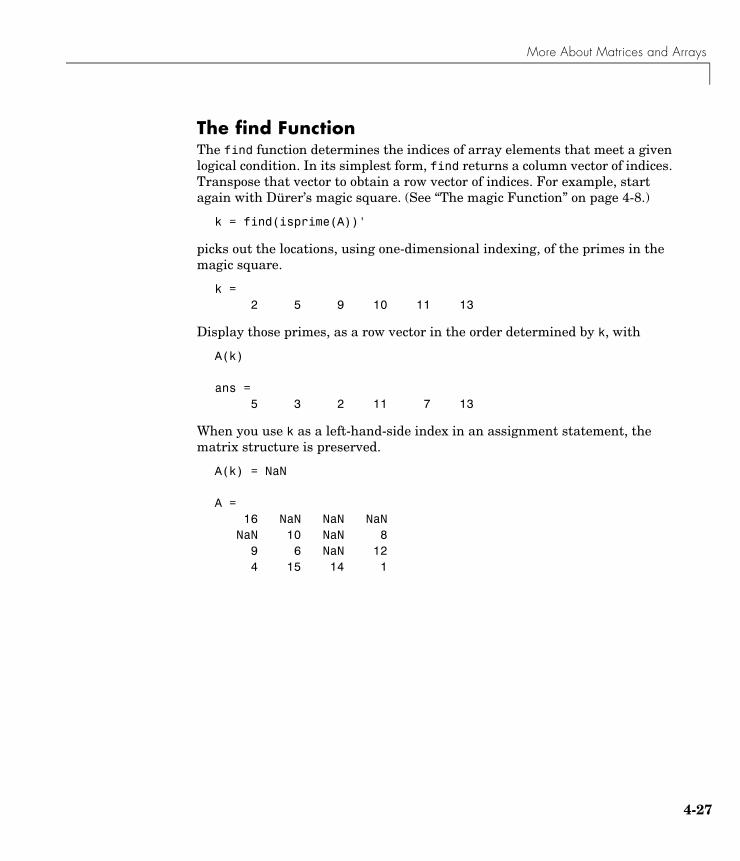
More About Matrices and Arrays
The find FunctionThe find function determines the indices of array elements that meet a given logical condition. In its simplest form, find returns a column vector of indices. Transpose that vector to obtain a row vector of indices. For example, start again with Dürer’s magic square. (See “The magic Function” on page 4-8.)
k = find(isprime(A))'
picks out the locations, using one-dimensional indexing, of the primes in the magic square.
k = 2 5 9 10 11 13
Display those primes, as a row vector in the order determined by k, with
A(k)
ans = 5 3 2 11 7 13
When you use k as a left-hand-side index in an assignment statement, the matrix structure is preserved.
A(k) = NaN
A = 16 NaN NaN NaN NaN 10 NaN 8 9 6 NaN 12 4 15 14 1
4-27
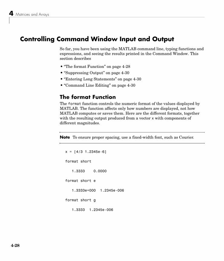
4 Matrices and Arrays
4-2
Controlling Command Window Input and OutputSo far, you have been using the MATLAB command line, typing functions and expressions, and seeing the results printed in the Command Window. This section describes
• “The format Function” on page 4-28
• “Suppressing Output” on page 4-30
• “Entering Long Statements” on page 4-30
• “Command Line Editing” on page 4-30
The format FunctionThe format function controls the numeric format of the values displayed by MATLAB. The function affects only how numbers are displayed, not how MATLAB computes or saves them. Here are the different formats, together with the resulting output produced from a vector x with components of different magnitudes.
Note To ensure proper spacing, use a fixed-width font, such as Courier.
x = [4/3 1.2345e-6]
format short
1.3333 0.0000
format short e
1.3333e+000 1.2345e-006
format short g
1.3333 1.2345e-006
8
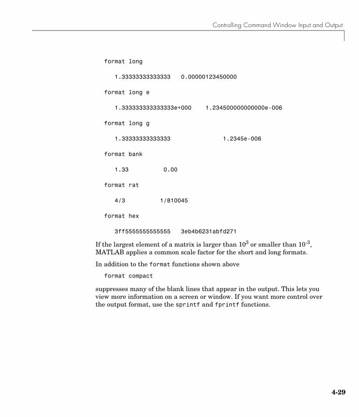
Controlling Command Window Input and Output
format long
1.33333333333333 0.00000123450000
format long e
1.333333333333333e+000 1.234500000000000e-006
format long g
1.33333333333333 1.2345e-006
format bank
1.33 0.00
format rat
4/3 1/810045
format hex
3ff5555555555555 3eb4b6231abfd271
If the largest element of a matrix is larger than 103 or smaller than 10-3, MATLAB applies a common scale factor for the short and long formats.
In addition to the format functions shown above
format compact
suppresses many of the blank lines that appear in the output. This lets you view more information on a screen or window. If you want more control over the output format, use the sprintf and fprintf functions.
4-29
4 Matrices and Arrays
4-3
Suppressing OutputIf you simply type a statement and press Return or Enter, MATLAB automatically displays the results on screen. However, if you end the line with a semicolon, MATLAB performs the computation but does not display any output. This is particularly useful when you generate large matrices. For example,
A = magic(100);
Entering Long StatementsIf a statement does not fit on one line, use an ellipsis (three periods), ..., followed by Return or Enter to indicate that the statement continues on the next line. For example,
s = 1 -1/2 + 1/3 -1/4 + 1/5 - 1/6 + 1/7 ... - 1/8 + 1/9 - 1/10 + 1/11 - 1/12;
Blank spaces around the =, +, and - signs are optional, but they improve readability.
Command Line EditingVarious arrow and control keys on your keyboard allow you to recall, edit, and reuse statements you have typed earlier. For example, suppose you mistakenly enter
rho = (1 + sqt(5))/2
You have misspelled sqrt. MATLAB responds with
Undefined function or variable 'sqt'.
Instead of retyping the entire line, simply press the ↑ key. The statement you typed is redisplayed. Use the ← key to move the cursor over and insert the missing r. Repeated use of the ↑ key recalls earlier lines. Typing a few characters and then the ↑ key finds a previous line that begins with those characters. You can also copy previously executed statements from the Command History. For more information, see “Command History” on page 8-5.
Following is the list of arrow and control keys you can use in the Command Window. If the preference you select for Command line key bindings is Emacs (MATLAB standard), you can also use the Ctrl+key combinations
0
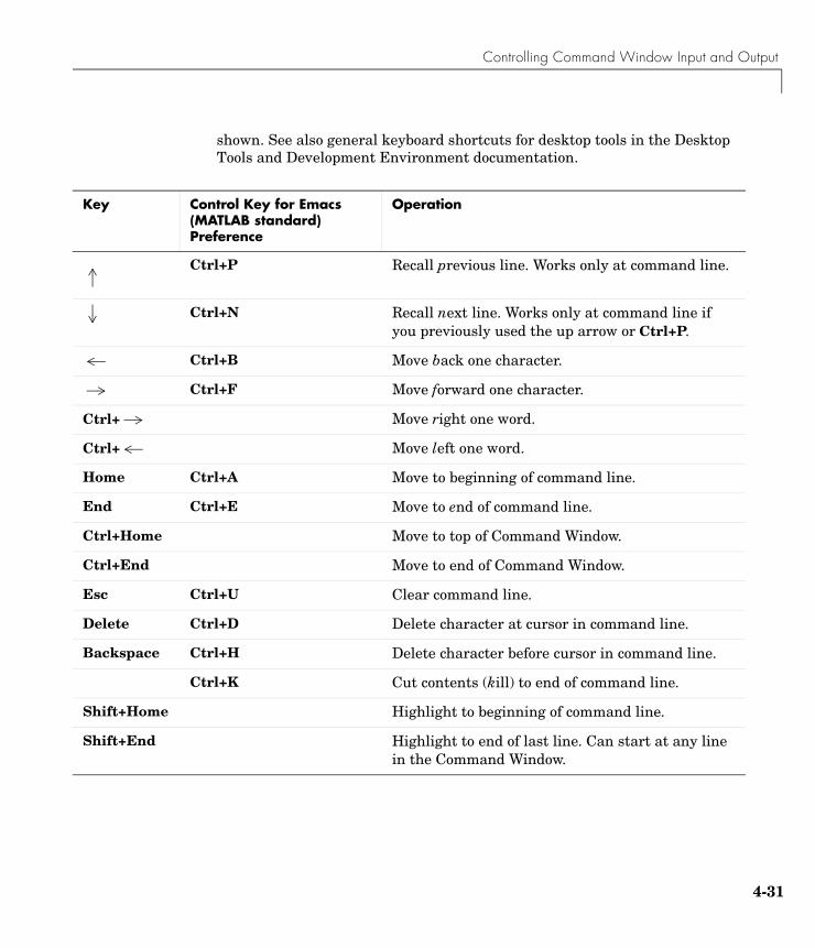
Controlling Command Window Input and Output
shown. See also general keyboard shortcuts for desktop tools in the Desktop Tools and Development Environment documentation.
Key Control Key for Emacs (MATLAB standard) Preference
Operation
Ctrl+P Recall previous line. Works only at command line.
Ctrl+N Recall next line. Works only at command line if you previously used the up arrow or Ctrl+P.
Ctrl+B Move back one character.
Ctrl+F Move forward one character.
Ctrl+ Move right one word.
Ctrl+ Move left one word.
Home Ctrl+A Move to beginning of command line.
End Ctrl+E Move to end of command line.
Ctrl+Home Move to top of Command Window.
Ctrl+End Move to end of Command Window.
Esc Ctrl+U Clear command line.
Delete Ctrl+D Delete character at cursor in command line.
Backspace Ctrl+H Delete character before cursor in command line.
Ctrl+K Cut contents (kill) to end of command line.
Shift+Home Highlight to beginning of command line.
Shift+End Highlight to end of last line. Can start at any line in the Command Window.
4-31

4 Matrices and Arrays
4-3
2
5
Graphics
This chapter provides an introduction to plotting data in MATLAB.
Overview of MATLAB Plotting (p. 5-2) Create plots, include multiple data sets, specify property values, and save figures.
Editing Plots (p. 5-16) Edit plots interactively and using functions, and use the property editor.
Mesh and Surface Plots (p. 5-52) Visualize functions of two variables.
Images (p. 5-58) Work with images.
Printing Graphics (p. 5-60) Print and export figures.
Handle Graphics (p. 5-62) Work with graphics objects and set object properties.
Animations (p. 5-71) Create moving graphics.
5 Graphics
5-2
Overview of MATLAB PlottingMATLAB provides a wide variety of techniques to display data graphically. Interactive tools enable you to manipulate graphs to achieve results that reveal the most information about your data. You can also annotate and print graphs for presentations, or export graphs to standard graphics formats for presentation in web browsers or other media.
For More Information “Graphics” and “3-D Visualization” in the MATLAB documentation provide in-depth coverage of MATLAB graphics and visualization tools. Access these topics from the Help browser.
The Plotting ProcessThe process of visualizing data typically involves a series of operations. This section provides a “big picture” view of the plotting process and contains links to sections that have examples and specific details about performing each operation.
Creating a GraphThe type of graph you choose to create depends on the nature of your data and what you want to reveal about the data. MATLAB predefines many graph types, such as line, bar, histogram, and pie graphs. There are also 3-D graphs, such as surfaces, slice planes, and streamlines.
There are two basic ways to create graphs in MATLAB:
• Use plotting tools to create graphs interactively.
See “Examples — Using MATLAB Plotting Tools” on page 5-20.
• Use the command interface to enter commands in the Command Window or create plotting programs.
See “Basic Plotting Functions” on page 5-38.
You might find it useful to combine both approaches. For example, you might issue a plotting command to create a graph and then modify the graph using one of the interactive tools.
Overview of MATLAB Plotting
Exploring DataOnce you create a graph, you can extract specific information about the data, such as the numeric value of a peak in a plot, the average value of a series of data, or you can perform data fitting.
For More Information See “Data Exploration Tools” and “Basic Fitting Options” in the MATLAB documentation.
Editing the Graph ComponentsGraphs are composed of objects, which have properties you can change. These properties affect the way the various graph components look and behave.
For example, the axes used to define the coordinate system of the graph has properties that define the limits of each axis, the scale, color, etc. The line used to create a line graph has properties such as color, type of marker used at each data point (if any), line style, etc.
Note that the data used to create a line graph are properties of the line. You can, therefore, change the data without actually creating a new graph.
See “Editing Plots” on page 5-16.
Annotating GraphsAnnotations are the text, arrows, callouts, and other labels added to graphs to help viewers see what is important about the data. You typically add annotations to graphs when you want to show them to other people or when you want to save them for later reference.
For More Information See “Annotating Graphs” in the MATLAB documentation or select Annotating Graphs from the figure Help menu.
5-3
5 Graphics
5-4
Printing and Exporting GraphsYou can print your graph on any printer connected to your computer. The print previewer enables you to view how your graph will look when printed. It enables you to add headers, footers, a date, and so on. The page setup dialog lets you control the size, layout, and other characteristics of the graph (select Page Setup from the figure File menu).
Exporting a graph means creating a copy of it in a standard graphics file format, such as TIF, JPEG, or EPS. You can then import the file into a word processor, include it in an HTML document, or edit it in a drawing package select Export Setup from the figure File menu).
For More Information See the print command reference page and “Printing and Exporting” in the MATLAB documentation or select Printing and Exporting from the figure Help menu.
Saving Graphs to Reload into MATLABThere are two ways to save graphs that enable you to save the work you have invested in their preparation:
• Save the graph as a FIG-file (select Save from the figure File menu).
• Generate MATLAB code that can recreate the graph (select Generate M-File from the figure File menu).
FIG-Files. FIG-files are a binary format that saves a figure in its current state. This means that all graphics objects and property settings are stored in the file when you create it. You can reload the file into a different MATLAB session, even if you are running MATLAB on a different type of computer. When you load a FIG-file, MATLAB creates a new figure in the same state as the one you saved.
Note that the states of any figure tools (i.e., any items on the toolbars) are not saved in a FIG-file; only the contents of the graph are saved.
Overview of MATLAB Plotting
Generated Code. You can use the MATLAB M-code generator to create code that recreates the graph. Unlike a FIG-file, the generated code does not contain any data. You must pass the data to the generated function when you run the code.
Note that studying the generating code for a graph is a good way to learn how to program with MATLAB.
For More Information See the print command reference page and “Saving Your Work” in the MATLAB documentation.
Graph ComponentsMATLAB displays graphs in a special window known as a figure. To create a graph, you need to define a coordinate system. Therefore every graph is placed within axes, which are contained by the figure.
The actual visual representation of the data is achieved with graphics objects like lines and surfaces. These objects are drawn within the coordinate system defined by the axes, which MATLAB automatically creates specifically to accommodate the range of the data. The actual data is stored as properties of the graphics objects.
See “Handle Graphics” on page 5-62 for more information about graphics object properties.
The following picture shows the basic components of a typical graph.
5-5
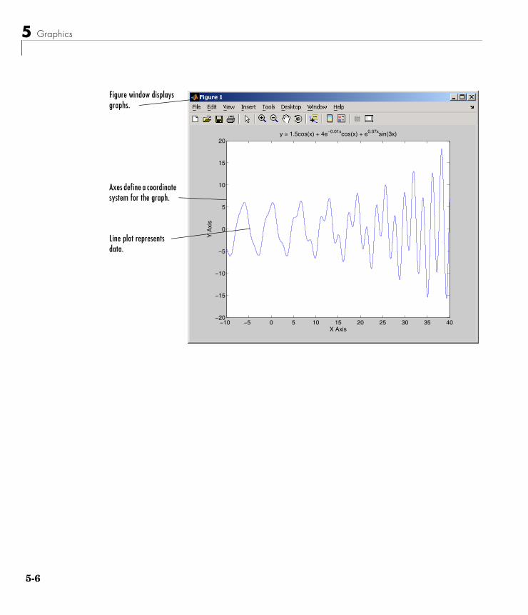
5 Graphics
5-6
−10 −5 0 5 10 15 20 25 30 35 40−20
−15
−10
−5
0
5
10
15
20y = 1.5cos(x) + 4e−0.01xcos(x) + e0.07xsin(3x)
X Axis
Y A
xis
Figure window displays graphs.
Axes define a coordinate system for the graph.
Line plot represents data.
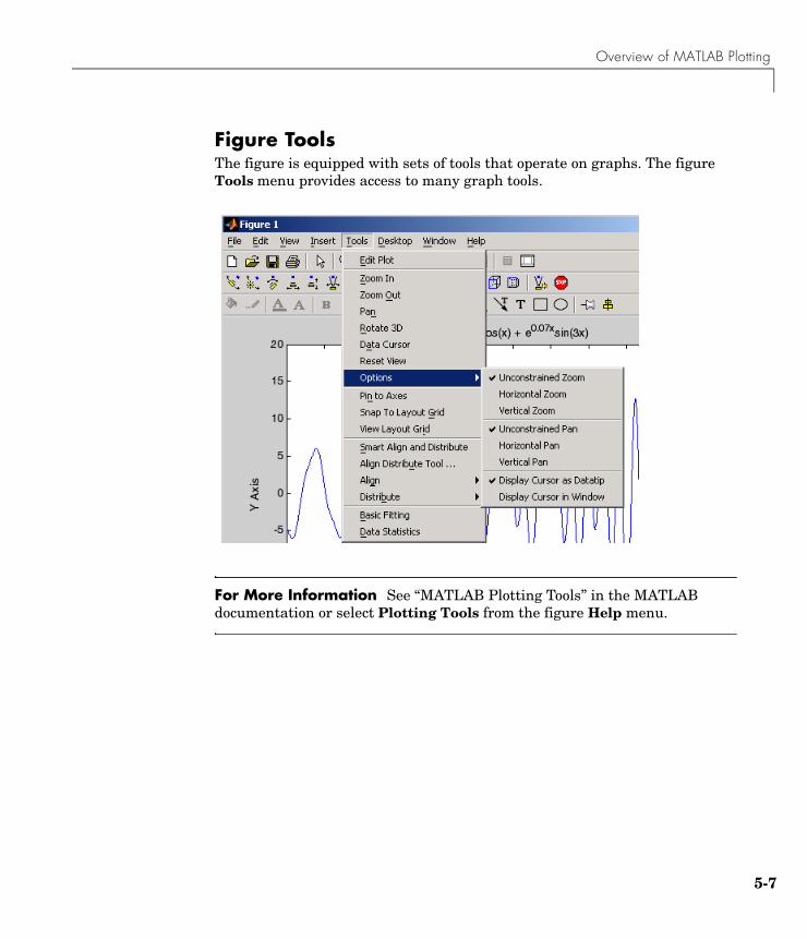
Overview of MATLAB Plotting
Figure ToolsThe figure is equipped with sets of tools that operate on graphs. The figure Tools menu provides access to many graph tools.
For More Information See “MATLAB Plotting Tools” in the MATLAB documentation or select Plotting Tools from the figure Help menu.
5-7
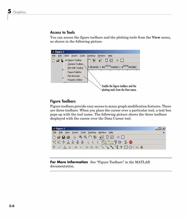
5 Graphics
5-8
Access to ToolsYou can access the figure toolbars and the plotting tools from the View menu, as shown in the following picture.
Figure ToolbarsFigure toolbars provide easy access to many graph modification features. There are three toolbars. When you place the cursor over a particular tool, a text box pops up with the tool name. The following picture shows the three toolbars displayed with the cursor over the Data Cursor tool.
For More Information See “Figure Toolbars” in the MATLAB documentation.
Enable the figure toolbars and the plotting tools from the View menu.
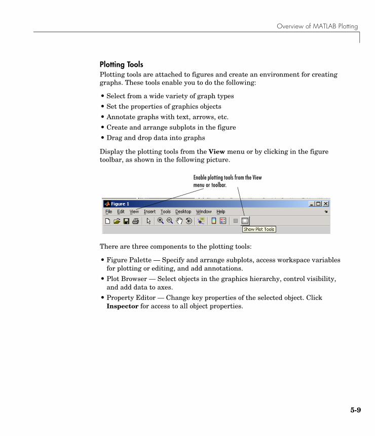
Overview of MATLAB Plotting
Plotting ToolsPlotting tools are attached to figures and create an environment for creating graphs. These tools enable you to do the following:
• Select from a wide variety of graph types
• Set the properties of graphics objects
• Annotate graphs with text, arrows, etc.
• Create and arrange subplots in the figure
• Drag and drop data into graphs
Display the plotting tools from the View menu or by clicking in the figure toolbar, as shown in the following picture.
There are three components to the plotting tools:
• Figure Palette — Specify and arrange subplots, access workspace variables for plotting or editing, and add annotations.
• Plot Browser — Select objects in the graphics hierarchy, control visibility, and add data to axes.
• Property Editor — Change key properties of the selected object. Click Inspector for access to all object properties.
Enable plotting tools from the View menu or toolbar.
5-9
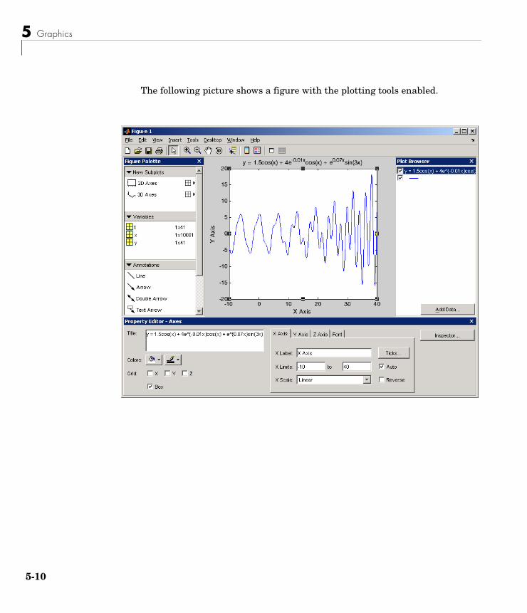
5 Graphics
5-1
The following picture shows a figure with the plotting tools enabled.
0
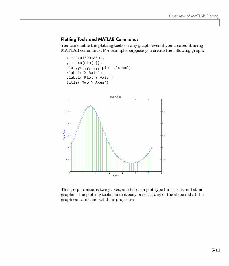
Overview of MATLAB Plotting
Plotting Tools and MATLAB Commands You can enable the plotting tools on any graph, even if you created it using MATLAB commands. For example, suppose you create the following graph.
t = 0:pi/20:2*pi;y = exp(sin(t));plotyy(t,y,t,y,'plot','stem')xlabel('X Axis')ylabel('Plot Y Axis')title('Two Y Axes')
This graph contains two y-axes, one for each plot type (lineseries and stem graphs). The plotting tools make it easy to select any of the objects that the graph contains and set their properties.
0 1 2 3 4 5 6 70
0.5
1
1.5
2
2.5
3
X Axis
Plo
t Y A
xis
Two Y Axes
0 1 2 3 4 5 6 70
0.5
1
1.5
2
2.5
3
5-11
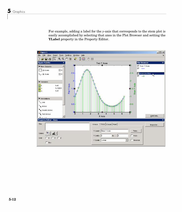
5 Graphics
5-1
For example, adding a label for the y-axis that corresponds to the stem plot is easily accomplished by selecting that axes in the Plot Browser and setting the YLabel property in the Property Editor.
2
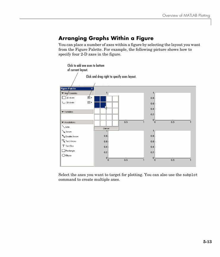
Overview of MATLAB Plotting
Arranging Graphs Within a FigureYou can place a number of axes within a figure by selecting the layout you want from the Figure Palette. For example, the following picture shows how to specify four 2-D axes in the figure.
Select the axes you want to target for plotting. You can also use the subplot command to create multiple axes.
Click to add one axes to bottom of current layout.
Click and drag right to specify axes layout.
5-13
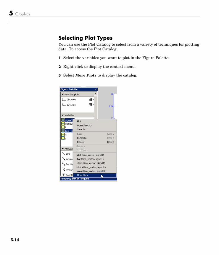
5 Graphics
5-1
Selecting Plot TypesYou can use the Plot Catalog to select from a variety of techniques for plotting data. To access the Plot Catalog,
1 Select the variables you want to plot in the Figure Palette.
2 Right-click to display the context menu.
3 Select More Plots to display the catalog.
4
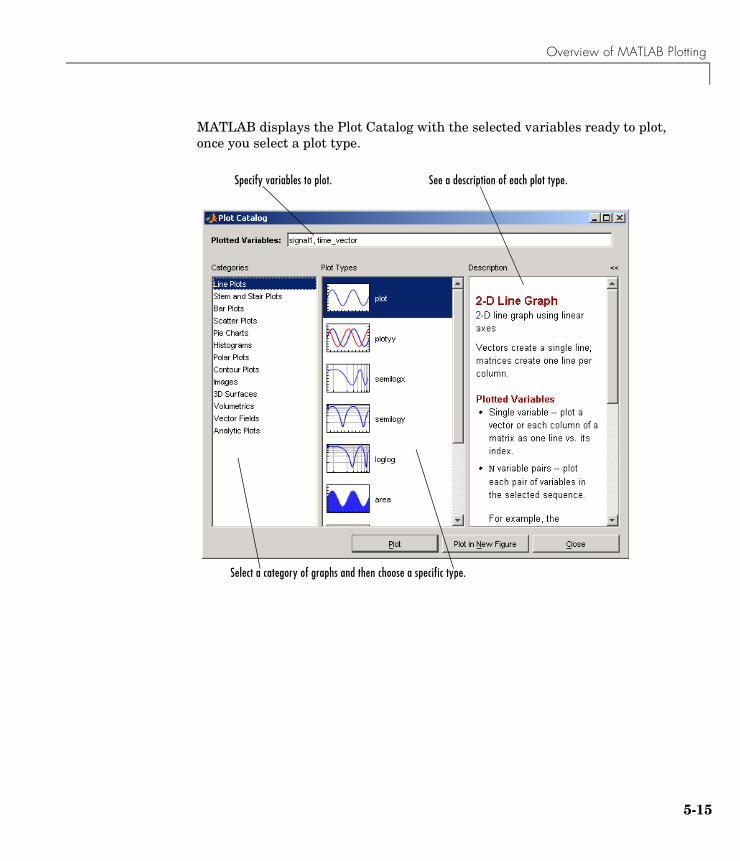
Overview of MATLAB Plotting
MATLAB displays the Plot Catalog with the selected variables ready to plot, once you select a plot type.
Specify variables to plot.
Select a category of graphs and then choose a specific type.
See a description of each plot type.
5-15
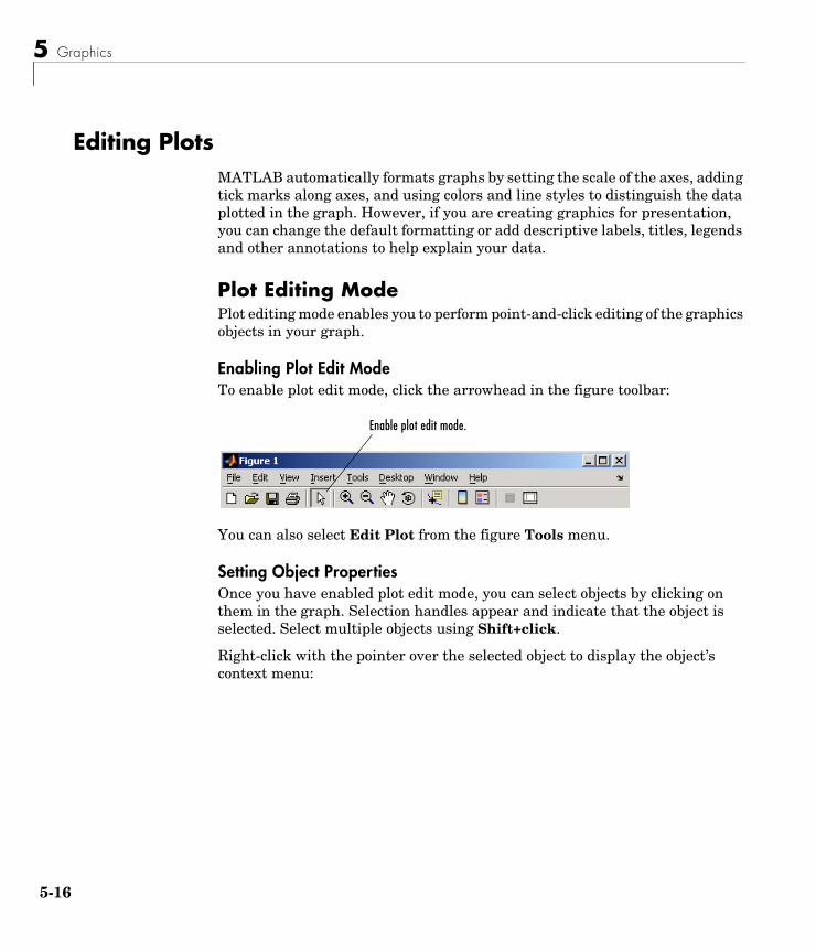
5 Graphics
5-1
Editing Plots MATLAB automatically formats graphs by setting the scale of the axes, adding tick marks along axes, and using colors and line styles to distinguish the data plotted in the graph. However, if you are creating graphics for presentation, you can change the default formatting or add descriptive labels, titles, legends and other annotations to help explain your data.
Plot Editing ModePlot editing mode enables you to perform point-and-click editing of the graphics objects in your graph.
Enabling Plot Edit ModeTo enable plot edit mode, click the arrowhead in the figure toolbar:
You can also select Edit Plot from the figure Tools menu.
Setting Object PropertiesOnce you have enabled plot edit mode, you can select objects by clicking on them in the graph. Selection handles appear and indicate that the object is selected. Select multiple objects using Shift+click.
Right-click with the pointer over the selected object to display the object’s context menu:
Enable plot edit mode.
6
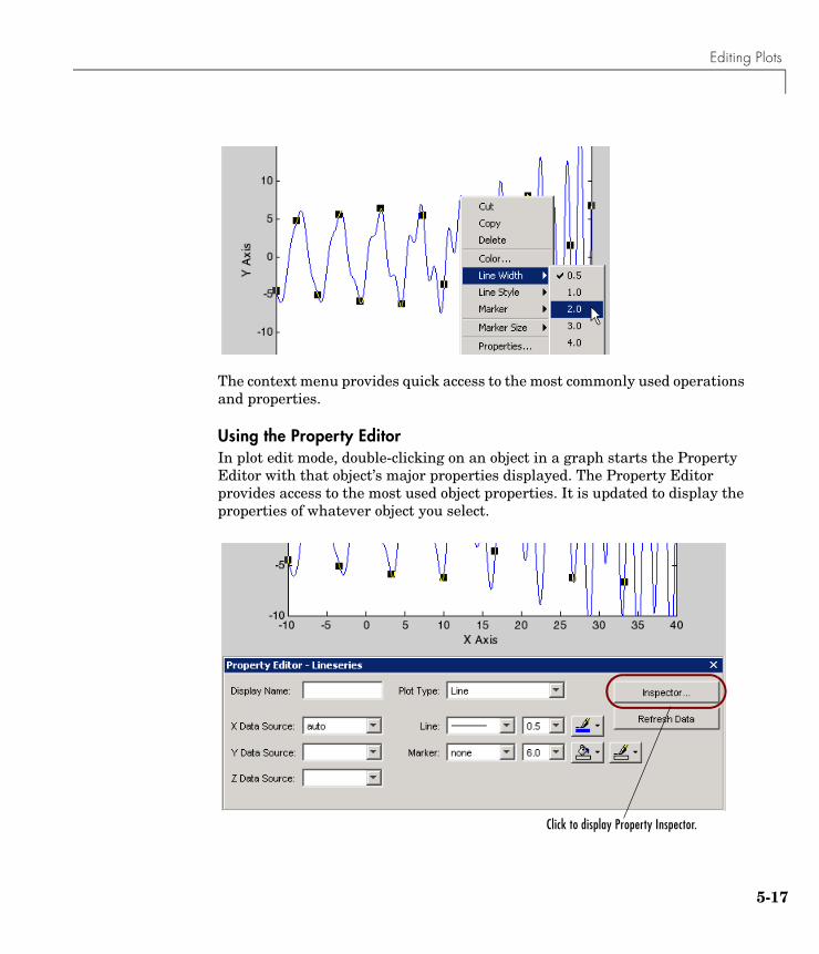
Editing Plots
The context menu provides quick access to the most commonly used operations and properties.
Using the Property EditorIn plot edit mode, double-clicking on an object in a graph starts the Property Editor with that object’s major properties displayed. The Property Editor provides access to the most used object properties. It is updated to display the properties of whatever object you select.
Click to display Property Inspector.
5-17
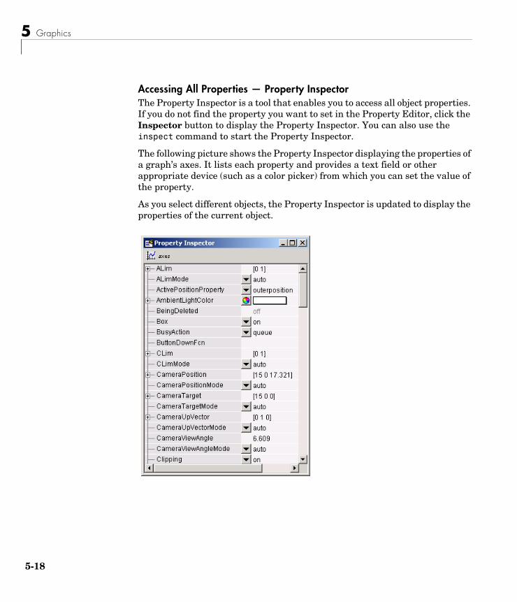
5 Graphics
5-1
Accessing All Properties — Property InspectorThe Property Inspector is a tool that enables you to access all object properties. If you do not find the property you want to set in the Property Editor, click the Inspector button to display the Property Inspector. You can also use the inspect command to start the Property Inspector.
The following picture shows the Property Inspector displaying the properties of a graph’s axes. It lists each property and provides a text field or other appropriate device (such as a color picker) from which you can set the value of the property.
As you select different objects, the Property Inspector is updated to display the properties of the current object.
8
Editing Plots
Using Functions to Edit GraphsIf you prefer to work from the MATLAB command line, or if you are creating an M-file, you can use MATLAB commands to edit the graphs you create. You can use the set and get commands to change the properties of the objects in a graph. For more information about using graphics commands, see “Handle Graphics” on page 5-62.
5-19
5 Graphics
5-2
Examples — Using MATLAB Plotting ToolsSuppose you want to graph the function y = x3 over the x domain -1 to 1. The first step is to generate the data to plot.
It is simple to evaluate a function because MATLAB can distribute arithmetic operations over all elements of a multivalued variable.
For example, the following statement creates a variable x that contains values ranging from -1 to 1 in increments of 0.1 (you could also use the linspace function to generate data for x). The second statement raises each value in x to the third power and stores these values in y.
x = -1:.1:1; % Define the range of xy = x.^3; % Raise each element in x to the third power
Now that you have generated some data, you can plot it using the MATLAB plotting tools. To start the plotting tools, type
plottools
0
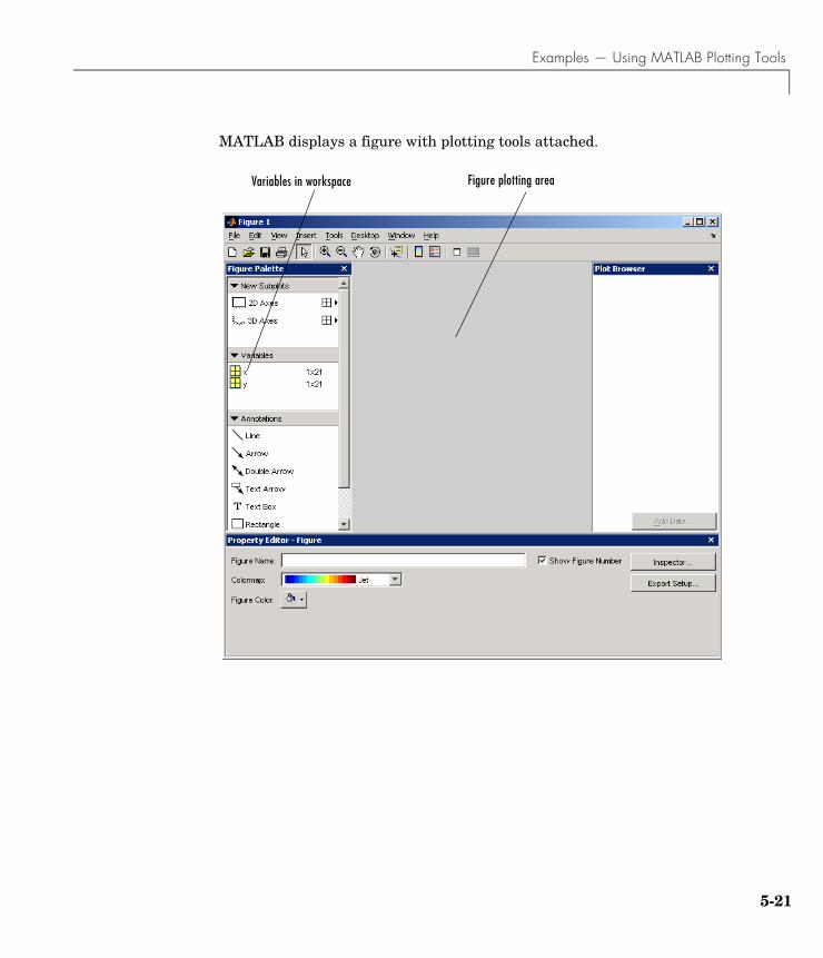
Examples — Using MATLAB Plotting Tools
MATLAB displays a figure with plotting tools attached.
Figure plotting areaVariables in workspace
5-21
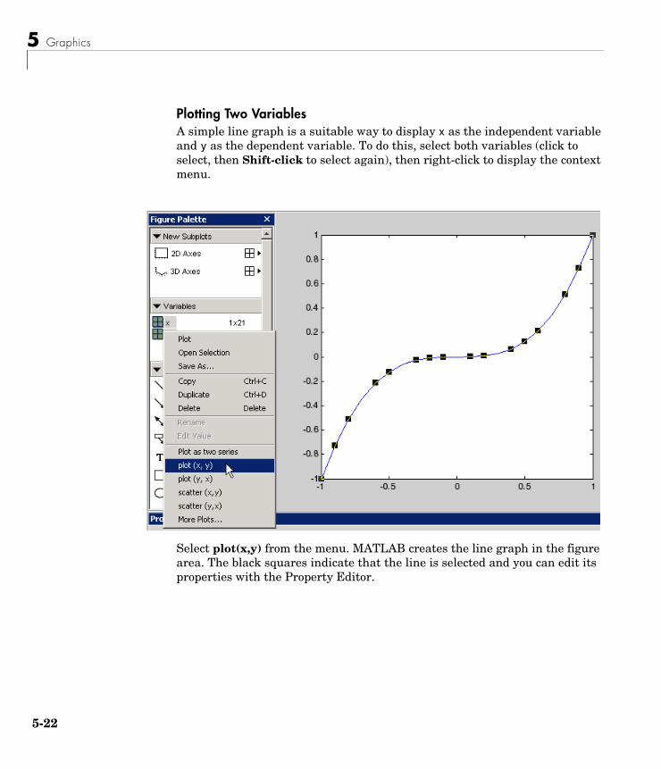
5 Graphics
5-2
Plotting Two VariablesA simple line graph is a suitable way to display x as the independent variable and y as the dependent variable. To do this, select both variables (click to select, then Shift-click to select again), then right-click to display the context menu.
Select plot(x,y) from the menu. MATLAB creates the line graph in the figure area. The black squares indicate that the line is selected and you can edit its properties with the Property Editor.
2
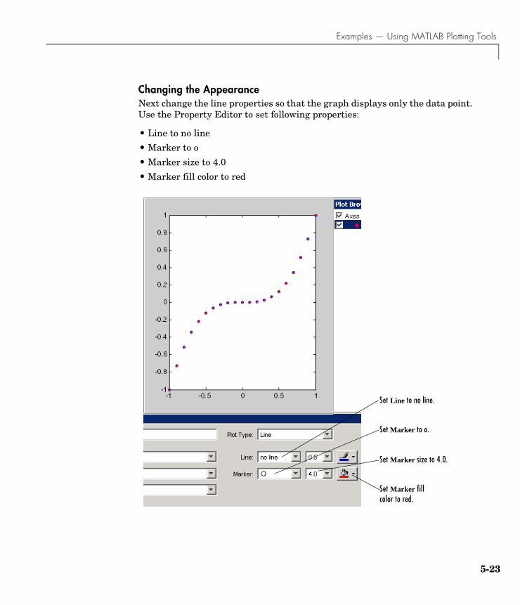
Examples — Using MATLAB Plotting Tools
Changing the Appearance Next change the line properties so that the graph displays only the data point. Use the Property Editor to set following properties:
• Line to no line
• Marker to o
• Marker size to 4.0
• Marker fill color to red
Set Line to no line.
Set Marker to o.
Set Marker size to 4.0.
Set Marker fill color to red.
5-23
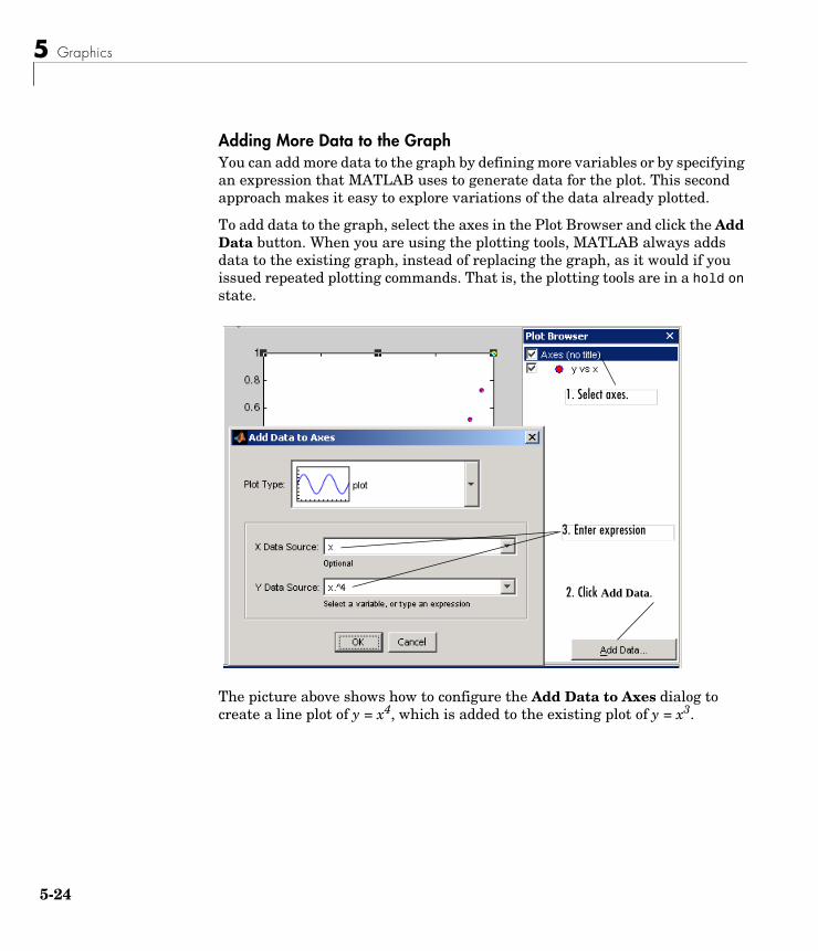
5 Graphics
5-2
Adding More Data to the GraphYou can add more data to the graph by defining more variables or by specifying an expression that MATLAB uses to generate data for the plot. This second approach makes it easy to explore variations of the data already plotted.
To add data to the graph, select the axes in the Plot Browser and click the Add Data button. When you are using the plotting tools, MATLAB always adds data to the existing graph, instead of replacing the graph, as it would if you issued repeated plotting commands. That is, the plotting tools are in a hold on state.
The picture above shows how to configure the Add Data to Axes dialog to create a line plot of y = x4, which is added to the existing plot of y = x3.
1. Select axes.
2. Click Add Data.
3. Enter expression
4
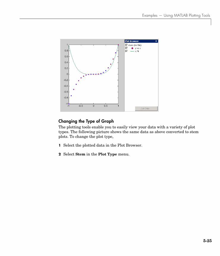
Examples — Using MATLAB Plotting Tools
Changing the Type of GraphThe plotting tools enable you to easily view your data with a variety of plot types. The following picture shows the same data as above converted to stem plots. To change the plot type,
1 Select the plotted data in the Plot Browser.
2 Select Stem in the Plot Type menu.
5-25
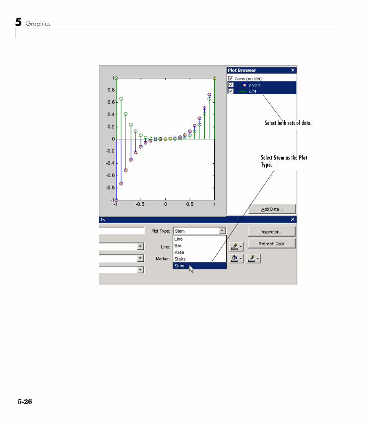
5 Graphics
5-2
Select both sets of data.
Select Stem as the Plot Type.
6
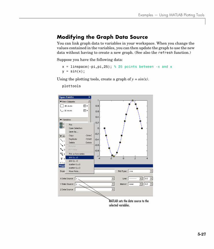
Examples — Using MATLAB Plotting Tools
Modifying the Graph Data SourceYou can link graph data to variables in your workspace. When you change the values contained in the variables, you can then update the graph to use the new data without having to create a new graph. (See also the refresh function.)
Suppose you have the following data:
x = linspace(-pi,pi,25); % 25 points between -π and πy = sin(x);
Using the plotting tools, create a graph of y = sin(x).
plottools
MATLAB sets the data source to the selected variables.
5-27
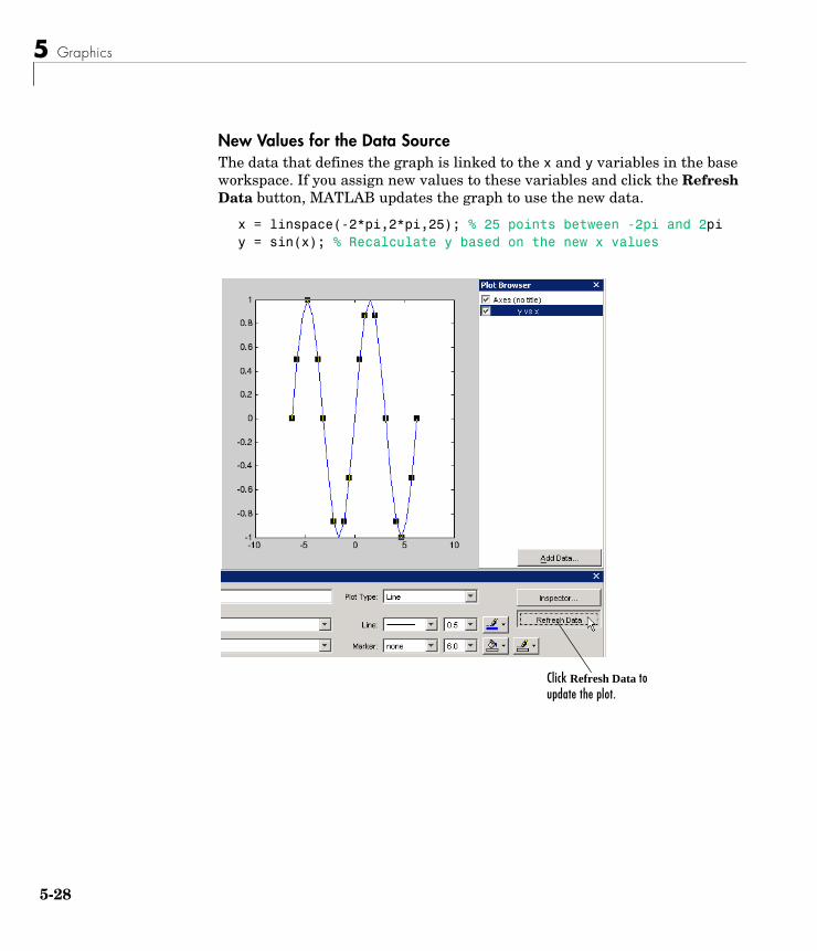
5 Graphics
5-2
New Values for the Data SourceThe data that defines the graph is linked to the x and y variables in the base workspace. If you assign new values to these variables and click the Refresh Data button, MATLAB updates the graph to use the new data.
x = linspace(-2*pi,2*pi,25); % 25 points between -2pi and 2piy = sin(x); % Recalculate y based on the new x values
Click Refresh Data to update the plot.
8
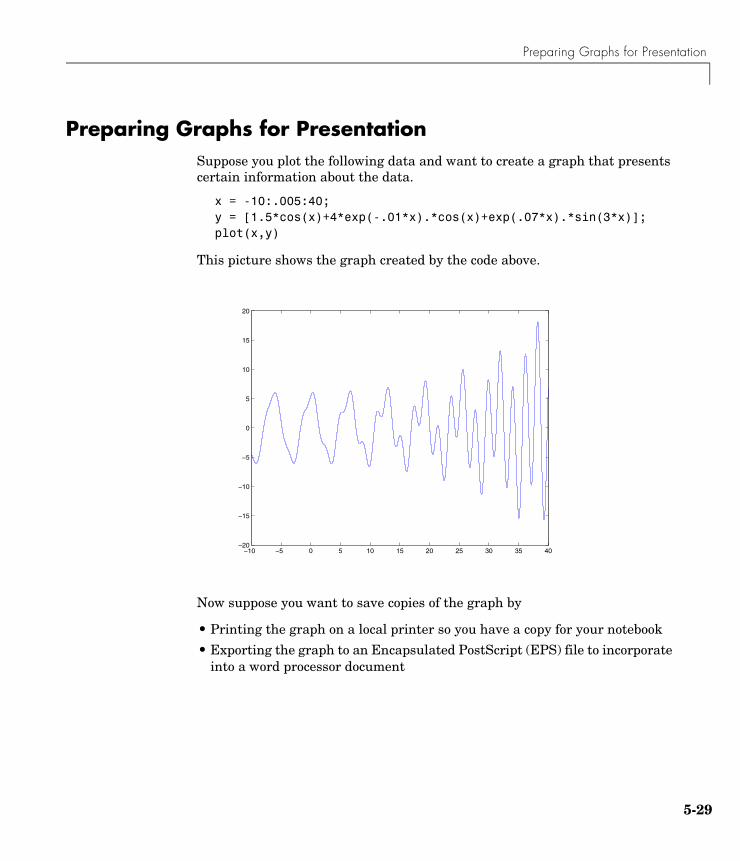
Preparing Graphs for Presentation
Preparing Graphs for PresentationSuppose you plot the following data and want to create a graph that presents certain information about the data.
x = -10:.005:40;y = [1.5*cos(x)+4*exp(-.01*x).*cos(x)+exp(.07*x).*sin(3*x)];plot(x,y)
This picture shows the graph created by the code above.
Now suppose you want to save copies of the graph by
• Printing the graph on a local printer so you have a copy for your notebook
• Exporting the graph to an Encapsulated PostScript (EPS) file to incorporate into a word processor document
−10 −5 0 5 10 15 20 25 30 35 40−20
−15
−10
−5
0
5
10
15
20
5-29
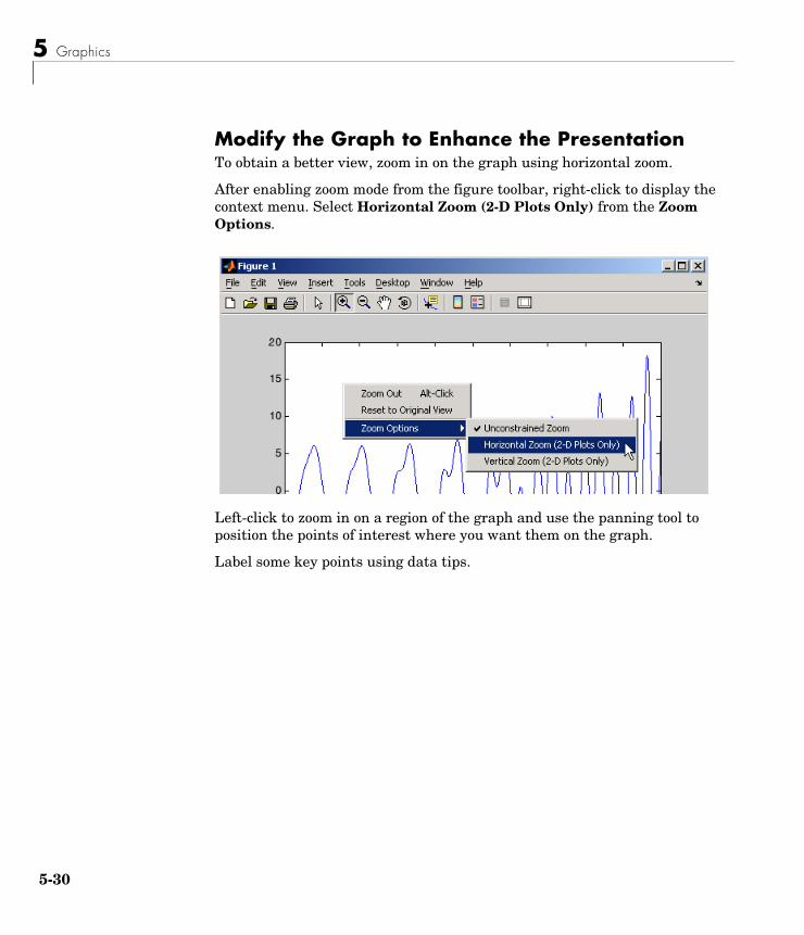
5 Graphics
5-3
Modify the Graph to Enhance the PresentationTo obtain a better view, zoom in on the graph using horizontal zoom.
After enabling zoom mode from the figure toolbar, right-click to display the context menu. Select Horizontal Zoom (2-D Plots Only) from the Zoom Options.
Left-click to zoom in on a region of the graph and use the panning tool to position the points of interest where you want them on the graph.
Label some key points using data tips.
0
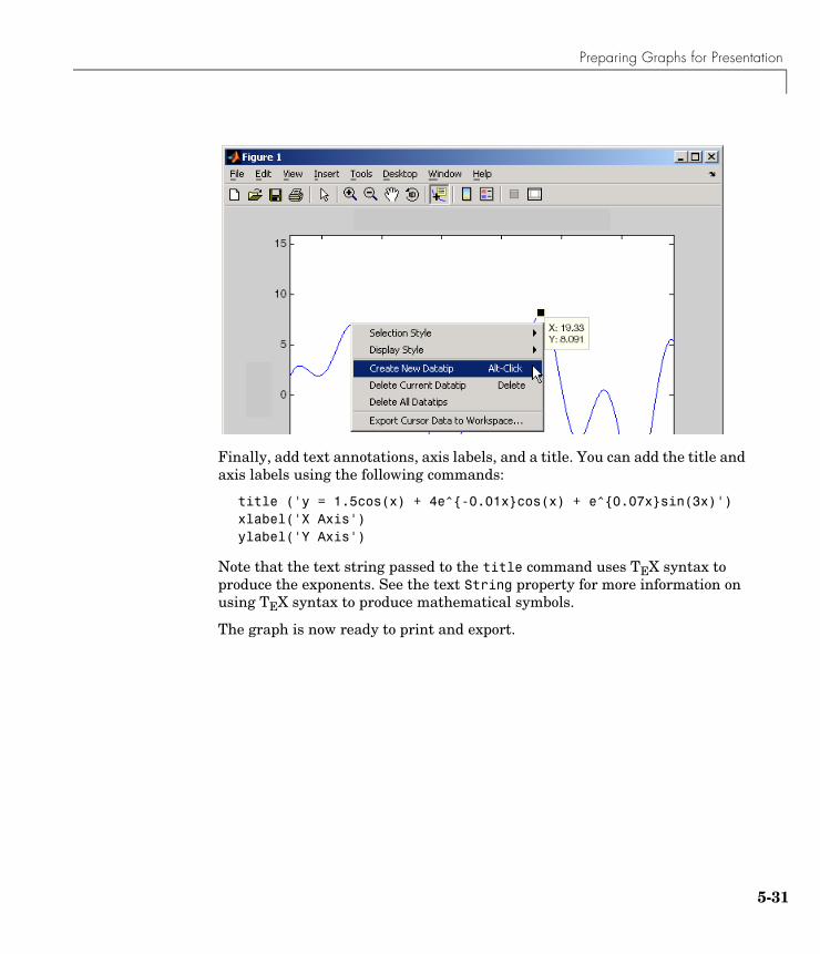
Preparing Graphs for Presentation
Finally, add text annotations, axis labels, and a title. You can add the title and axis labels using the following commands:
title ('y = 1.5cos(x) + 4e^{-0.01x}cos(x) + e^{0.07x}sin(3x)')xlabel('X Axis')ylabel('Y Axis')
Note that the text string passed to the title command uses TEX syntax to produce the exponents. See the text String property for more information on using TEX syntax to produce mathematical symbols.
The graph is now ready to print and export.
5-31
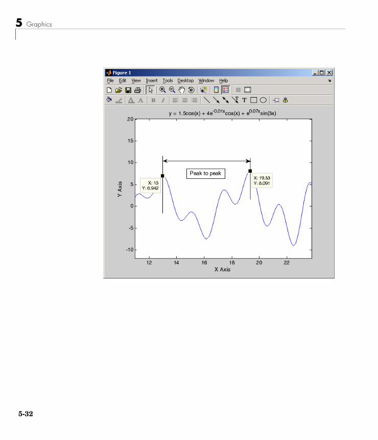
5 Graphics
5-3
2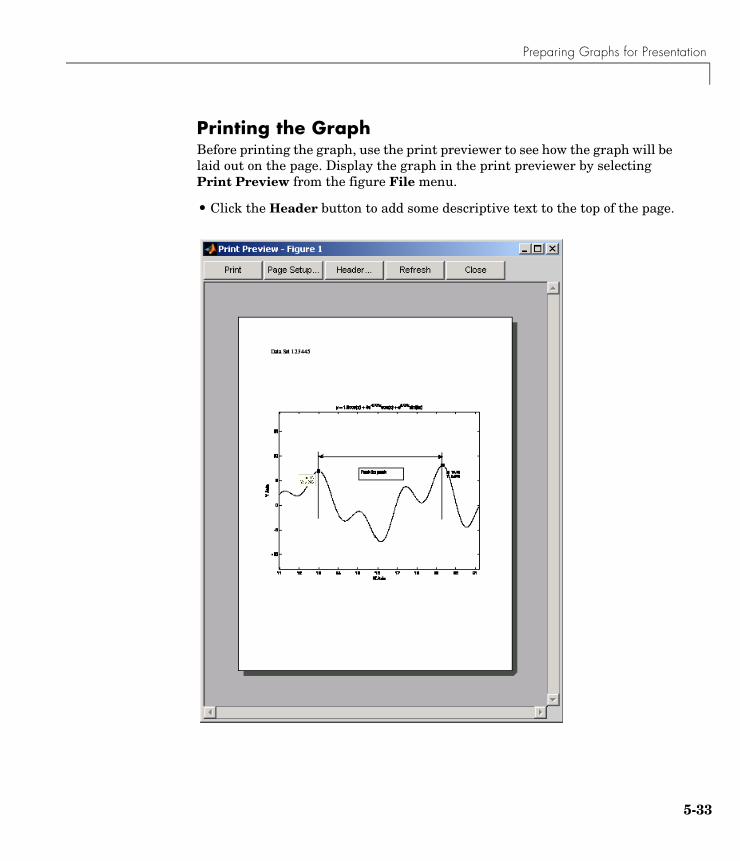
Preparing Graphs for Presentation
Printing the GraphBefore printing the graph, use the print previewer to see how the graph will be laid out on the page. Display the graph in the print previewer by selecting Print Preview from the figure File menu.
• Click the Header button to add some descriptive text to the top of the page.
5-33
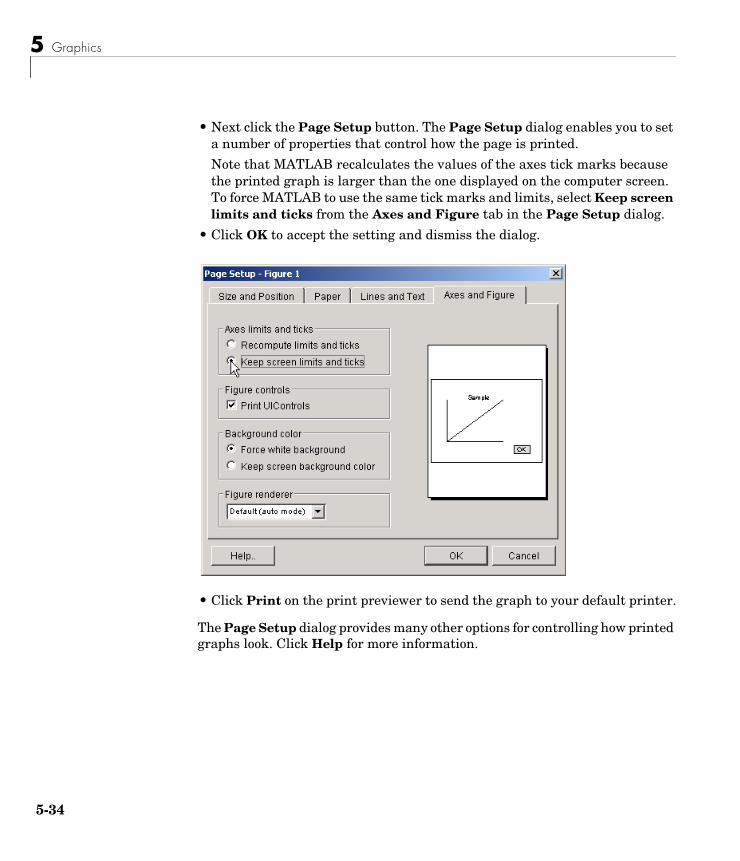
5 Graphics
5-3
• Next click the Page Setup button. The Page Setup dialog enables you to set a number of properties that control how the page is printed.
Note that MATLAB recalculates the values of the axes tick marks because the printed graph is larger than the one displayed on the computer screen. To force MATLAB to use the same tick marks and limits, select Keep screen limits and ticks from the Axes and Figure tab in the Page Setup dialog.
• Click OK to accept the setting and dismiss the dialog.
• Click Print on the print previewer to send the graph to your default printer.
The Page Setup dialog provides many other options for controlling how printed graphs look. Click Help for more information.
4
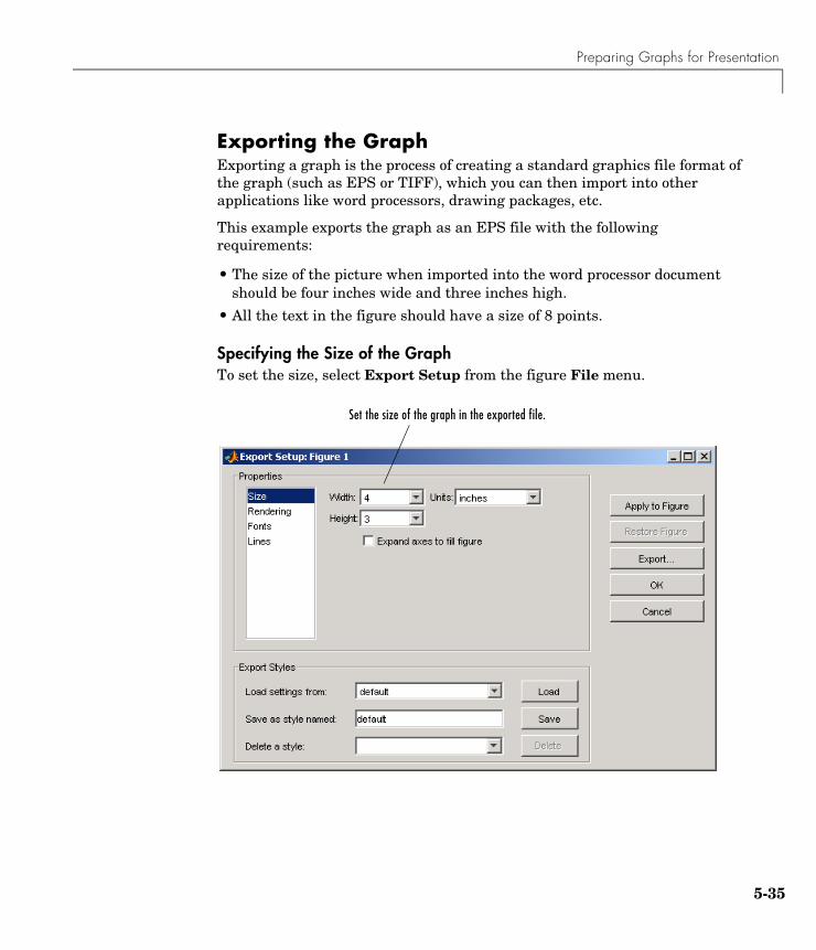
Preparing Graphs for Presentation
Exporting the GraphExporting a graph is the process of creating a standard graphics file format of the graph (such as EPS or TIFF), which you can then import into other applications like word processors, drawing packages, etc.
This example exports the graph as an EPS file with the following requirements:
• The size of the picture when imported into the word processor document should be four inches wide and three inches high.
• All the text in the figure should have a size of 8 points.
Specifying the Size of the GraphTo set the size, select Export Setup from the figure File menu.
Set the size of the graph in the exported file.
5-35
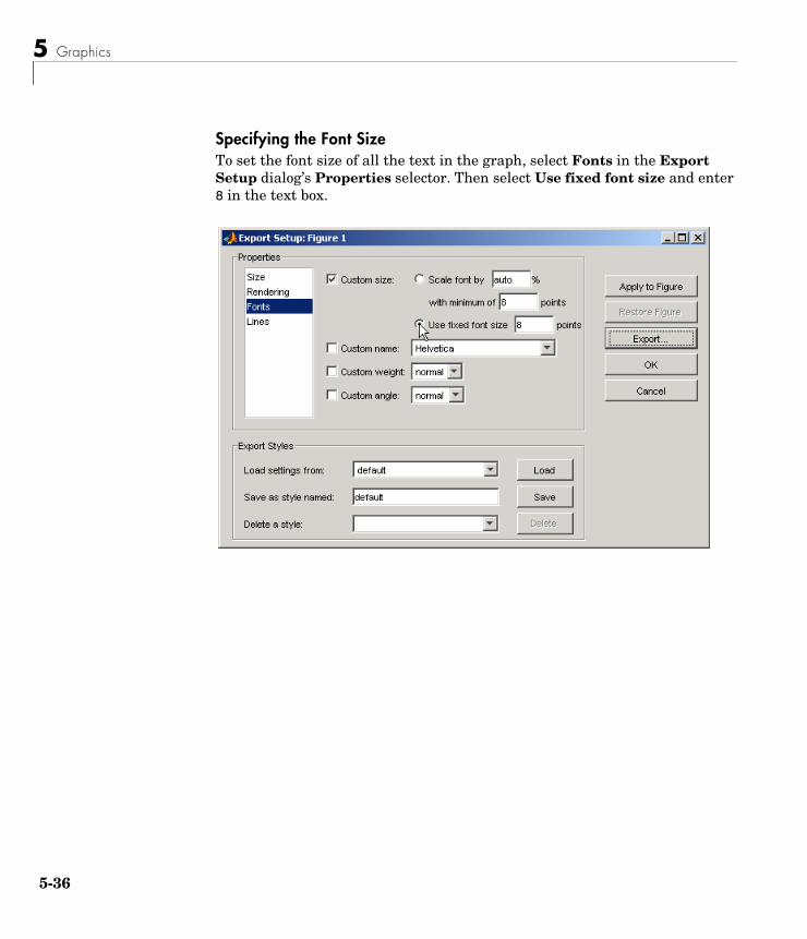
5 Graphics
5-3
Specifying the Font SizeTo set the font size of all the text in the graph, select Fonts in the Export Setup dialog’s Properties selector. Then select Use fixed font size and enter 8 in the text box.
6
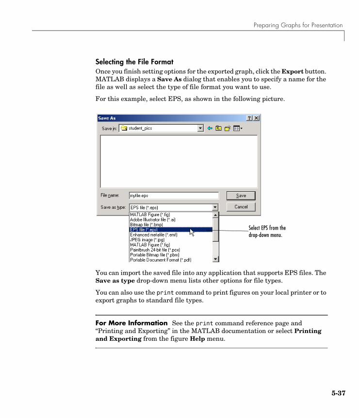
Preparing Graphs for Presentation
Selecting the File FormatOnce you finish setting options for the exported graph, click the Export button. MATLAB displays a Save As dialog that enables you to specify a name for the file as well as select the type of file format you want to use.
For this example, select EPS, as shown in the following picture.
You can import the saved file into any application that supports EPS files. The Save as type drop-down menu lists other options for file types.
You can also use the print command to print figures on your local printer or to export graphs to standard file types.
For More Information See the print command reference page and “Printing and Exporting” in the MATLAB documentation or select Printing and Exporting from the figure Help menu.
Select EPS from the drop-down menu.
5-37
5 Graphics
5-3
Basic Plotting FunctionsThis section describes important graphics functions and provides examples of some typical applications. The plotting tools, described in previous sections, make use of MATLAB plotting functions and use these functions to generate code for graphs.
• “Creating a Plot” on page 5-38
• “Multiple Data Sets in One Graph” on page 5-40
• “Specifying Line Styles and Colors” on page 5-41
• “Plotting Lines and Markers” on page 5-41
• “Imaginary and Complex Data” on page 5-43
• “Adding Plots to an Existing Graph” on page 5-44
• “Figure Windows” on page 5-46
• “Multiple Plots in One Figure” on page 5-46
• “Controlling the Axes” on page 5-48
• “Axis Labels and Titles” on page 5-49
• “Saving Figures” on page 5-51
Creating a PlotThe plot function has different forms, depending on the input arguments. If y is a vector, plot(y) produces a piecewise linear graph of the elements of y versus the index of the elements of y. If you specify two vectors as arguments, plot(x,y) produces a graph of y versus x.
For example, these statements use the colon operator to create a vector of x values ranging from 0 to 2π, compute the sine of these values, and plot the result.
x = 0:pi/100:2*pi;y = sin(x);plot(x,y)
8
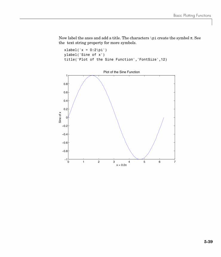
Basic Plotting Functions
Now label the axes and add a title. The characters \pi create the symbol π. See the text string property for more symbols.
xlabel('x = 0:2\pi')ylabel('Sine of x')title('Plot of the Sine Function','FontSize',12)
0 1 2 3 4 5 6 7−1
−0.8
−0.6
−0.4
−0.2
0
0.2
0.4
0.6
0.8
1
x = 0:2π
Sin
e of
x
Plot of the Sine Function
5-39
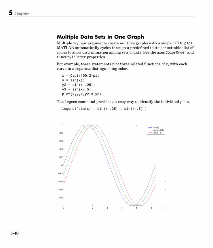
5 Graphics
5-4
Multiple Data Sets in One GraphMultiple x-y pair arguments create multiple graphs with a single call to plot. MATLAB automatically cycles through a predefined (but user settable) list of colors to allow discrimination among sets of data. See the axes ColorOrder and LineStyleOrder properties.
For example, these statements plot three related functions of x, with each curve in a separate distinguishing color.
x = 0:pi/100:2*pi;y = sin(x);y2 = sin(x-.25);y3 = sin(x-.5);plot(x,y,x,y2,x,y3)
The legend command provides an easy way to identify the individual plots.
legend('sin(x)','sin(x-.25)','sin(x-.5)')
0 1 2 3 4 5 6 7−1
−0.8
−0.6
−0.4
−0.2
0
0.2
0.4
0.6
0.8
1sin(x) sin(x−.25)sin(x−.5)
0
Basic Plotting Functions
For More Information See “Defining the Color of Lines for Plotting” in “Axes Properties” in the MATLAB documentation.
Specifying Line Styles and ColorsIt is possible to specify color, line styles, and markers (such as plus signs or circles) when you plot your data using the plot command.
plot(x,y,'color_style_marker')
color_style_marker is a string containing from one to four characters (enclosed in single quotation marks) constructed from a color, a line style, and a marker type:
• Color strings are 'c', 'm', 'y', 'r', 'g', 'b', 'w', and 'k'. These correspond to cyan, magenta, yellow, red, green, blue, white, and black.
• Line style strings are '-' for solid, '--' for dashed, ':' for dotted, '-.' for dash-dot. Omit the line style for no line.
• The marker types are '+', 'o', '*', and 'x', and the filled marker types are 's' for square, 'd' for diamond, '^' for up triangle, 'v' for down triangle, '>' for right triangle, '<' for left triangle, 'p' for pentagram, 'h' for hexagram, and none for no marker.
You can also edit color, line style, and markers interactively. See “Editing Plots” on page 5-16 for more information.
Plotting Lines and MarkersIf you specify a marker type but not a line style, MATLAB draws only the marker. For example,
plot(x,y,'ks')
plots black squares at each data point, but does not connect the markers with a line.
5-41
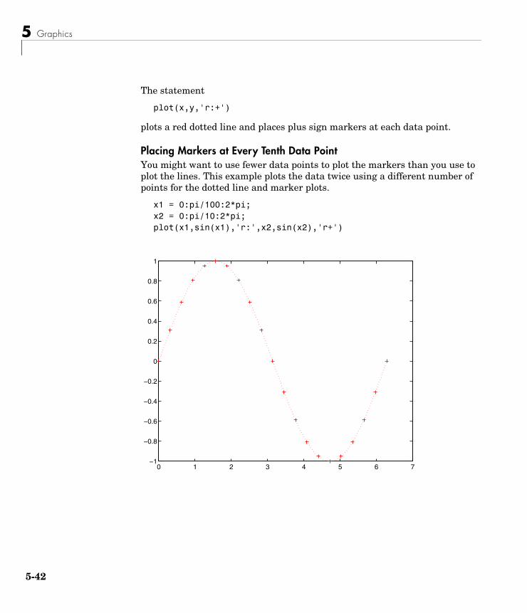
5 Graphics
5-4
The statement
plot(x,y,'r:+')
plots a red dotted line and places plus sign markers at each data point.
Placing Markers at Every Tenth Data PointYou might want to use fewer data points to plot the markers than you use to plot the lines. This example plots the data twice using a different number of points for the dotted line and marker plots.
x1 = 0:pi/100:2*pi;x2 = 0:pi/10:2*pi;plot(x1,sin(x1),'r:',x2,sin(x2),'r+')
0 1 2 3 4 5 6 7−1
−0.8
−0.6
−0.4
−0.2
0
0.2
0.4
0.6
0.8
1
2
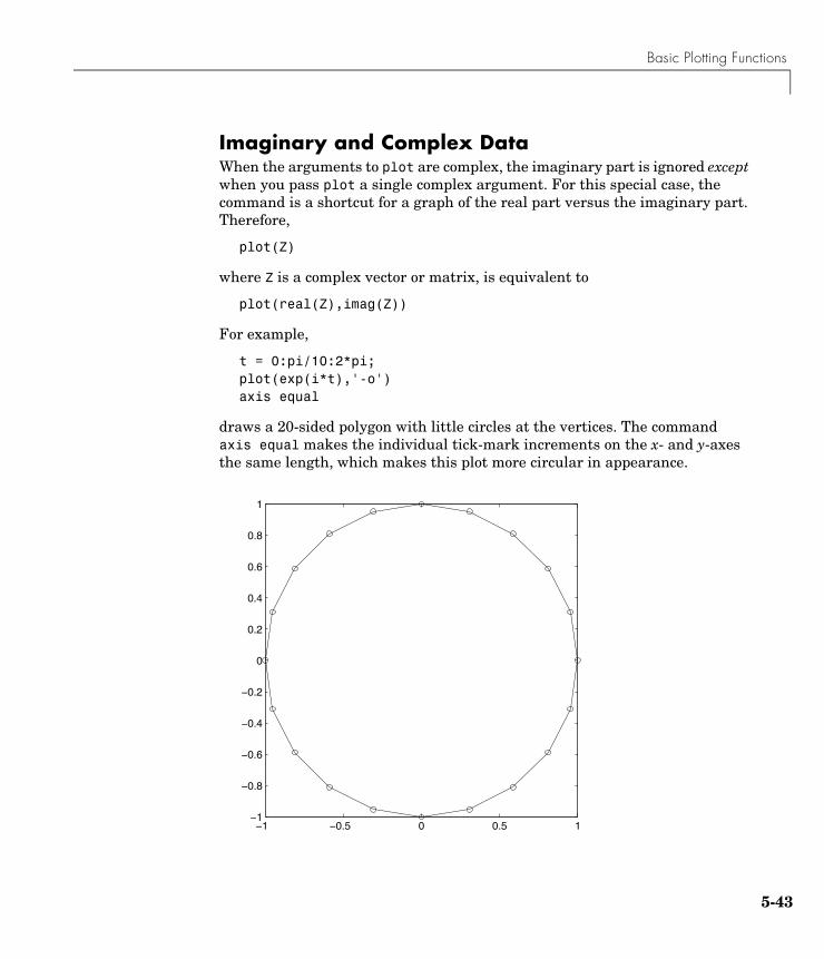
Basic Plotting Functions
Imaginary and Complex DataWhen the arguments to plot are complex, the imaginary part is ignored except when you pass plot a single complex argument. For this special case, the command is a shortcut for a graph of the real part versus the imaginary part. Therefore,
plot(Z)
where Z is a complex vector or matrix, is equivalent to
plot(real(Z),imag(Z))
For example,
t = 0:pi/10:2*pi;plot(exp(i*t),'-o')axis equal
draws a 20-sided polygon with little circles at the vertices. The command axis equal makes the individual tick-mark increments on the x- and y-axes the same length, which makes this plot more circular in appearance.
−1 −0.5 0 0.5 1−1
−0.8
−0.6
−0.4
−0.2
0
0.2
0.4
0.6
0.8
1
5-43
5 Graphics
5-4
Adding Plots to an Existing GraphThe hold command enables you to add plots to an existing graph. When you type
hold on
MATLAB does not replace the existing graph when you issue another plotting command; it adds the new data to the current graph, rescaling the axes if necessary.
For example, these statements first create a contour plot of the peaks function, then superimpose a pseudocolor plot of the same function.
[x,y,z] = peaks;pcolor(x,y,z)shading interphold oncontour(x,y,z,20,'k')hold off
The hold on command causes the pcolor plot to be combined with the contour plot in one figure.
4
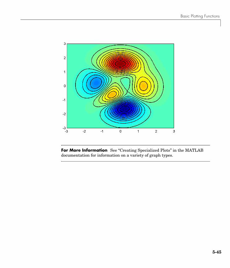
Basic Plotting Functions
For More Information See “Creating Specialized Plots” in the MATLAB documentation for information on a variety of graph types.
5-45
5 Graphics
5-4
Figure Windows Graphing functions automatically open a new figure window if there are no figure windows already on the screen. If a figure window exists, MATLAB uses that window for graphics output. If there are multiple figure windows open, MATLAB targets the one that is designated the “current figure” (the last figure used or clicked in).
To make an existing figure window the current figure, you can click the mouse while the pointer is in that window or you can type
figure(n)
where n is the number in the figure title bar. The results of subsequent graphics commands are displayed in this window.
To open a new figure window and make it the current figure, type
figure
Clearing the Figure for a New PlotWhen a figure already exists, most plotting commands clear the axes and use this figure to create the new plot. However, these commands do not reset figure properties, such as the background color or the colormap. If you have set any figure properties in the previous plot, you might want to use the clf command with the reset option,
clf reset
before creating your new plot to restore the figure’s properties to their defaults.
For More Information See “Figure Properties” and “Graphics Window — the Figure” in the MATLAB documentation for information on figures.
Multiple Plots in One FigureThe subplot command enables you to display multiple plots in the same window or print them on the same piece of paper. Typing
subplot(m,n,p)
6
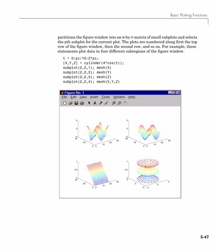
Basic Plotting Functions
partitions the figure window into an m-by-n matrix of small subplots and selects the pth subplot for the current plot. The plots are numbered along first the top row of the figure window, then the second row, and so on. For example, these statements plot data in four different subregions of the figure window.
t = 0:pi/10:2*pi;[X,Y,Z] = cylinder(4*cos(t));subplot(2,2,1); mesh(X)subplot(2,2,2); mesh(Y)subplot(2,2,3); mesh(Z)subplot(2,2,4); mesh(X,Y,Z)
010
2030
0
20
40−5
0
5
010
2030
0
20
40−5
0
5
010
2030
0
20
400
0.5
1
−50
5
−5
0
50
0.5
1
5-47
5 Graphics
5-4
Controlling the AxesThe axis command provides a number of options for setting the scaling, orientation, and aspect ratio of graphs. You can also set these options interactively. See “Editing Plots” on page 5-16 for more information.
Setting Axis LimitsBy default, MATLAB finds the maxima and minima of the data and chooses the axis limits to span this range. The axis command enables you to specify your own limits:
axis([xmin xmax ymin ymax])
or for three-dimensional graphs,
axis([xmin xmax ymin ymax zmin zmax])
Use the command
axis auto
to reenable MATLAB automatic limit selection.
Setting Axis Aspect Ratioaxis also enables you to specify a number of predefined modes. For example,
axis square
makes the x-axis and y-axis the same length.
axis equal
makes the individual tick mark increments on the x-axes and y-axes the same length. This means
plot(exp(i*[0:pi/10:2*pi]))
followed by either axis square or axis equal turns the oval into a proper circle.
axis auto normal
returns the axis scaling to its default automatic mode.
8
Basic Plotting Functions
Setting Axis VisibilityYou can use the axis command to make the axis visible or invisible.
axis on
makes the axes visible. This is the default.
axis off
makes the axes invisible.
Setting Grid LinesThe grid command toggles grid lines on and off. The statement
grid on
turns the grid lines on, and
grid off
turns them back off again.
For More Information See the axis and axes reference pages and “Axes Properties” in the MATLAB documentation.
Axis Labels and TitlesThe xlabel, ylabel, and zlabel commands add x-, y-, and z-axis labels. The title command adds a title at the top of the figure and the text function inserts text anywhere in the figure.
5-49
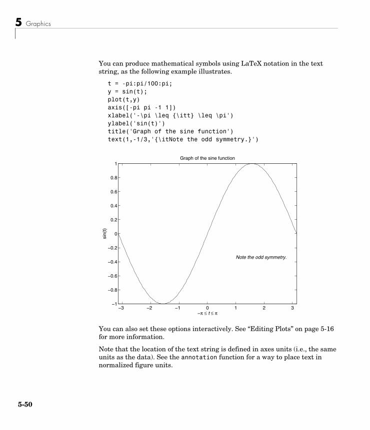
5 Graphics
5-5
You can produce mathematical symbols using LaTeX notation in the text string, as the following example illustrates.
t = -pi:pi/100:pi;y = sin(t);plot(t,y)axis([-pi pi -1 1])xlabel('-\pi \leq {\itt} \leq \pi')ylabel('sin(t)')title('Graph of the sine function')text(1,-1/3,'{\itNote the odd symmetry.}')
You can also set these options interactively. See “Editing Plots” on page 5-16 for more information.
Note that the location of the text string is defined in axes units (i.e., the same units as the data). See the annotation function for a way to place text in normalized figure units.
−3 −2 −1 0 1 2 3−1
−0.8
−0.6
−0.4
−0.2
0
0.2
0.4
0.6
0.8
1
−π ≤ t ≤ π
sin(
t)
Graph of the sine function
Note the odd symmetry.
0
Basic Plotting Functions
Saving FiguresSave a figure by selecting Save from the File menu to display a file save dialog. MATLAB saves the data it needs to recreate the figure and its contents (i.e., the entire graph) in a file with a .fig extension.
To save a figure using a standard graphics format, such as TIFF, for use with other applications, select Export Setup from the File menu. You can also save from the command line — use the saveas command, including any options to save the figure in a different format.
See “Exporting the Graph” on page 5-35 for an example.
Saving Workspace DataYou can save the variables in your workspace using the Save Workspace As item in the figure File menu. You can reload saved data using the Import Data item in the figure File menu. MATLAB supports a variety of data file formats, including MATLAB data files, which have a .mat extension.
Generating M-Code to Recreate a FigureYou can generate MATLAB code that recreates a figure and the graph it contains by selecting the Generate M-File item from the figure File menu. This option is particularly useful if you have developed a graph using plotting tools and want to create a similar graph using the same or different data.
Saving Figures That Are Compatible with Previous Version of MATLABCreate backward-compatible FIG-files by following these two steps.
• Ensure that any plotting functions used to create the contents of the figure are called with the 'v6' argument, where applicable.
• Use the '-v6' option with the hgsave command.
For More Information See “Plot Objects and Backward Compatibility” in the MATLAB documentation more information.
5-51
5 Graphics
5-5
Mesh and Surface PlotsMATLAB defines a surface by the z-coordinates of points above a grid in the x-y plane, using straight lines to connect adjacent points. The mesh and surf plotting functions display surfaces in three dimensions. mesh produces wireframe surfaces that color only the lines connecting the defining points. surf displays both the connecting lines and the faces of the surface in color.
The figure colormap and figure properties determine how MATLAB colors the surface.
Visualizing Functions of Two VariablesTo display a function of two variables, z = f (x,y),
• Generate X and Y matrices consisting of repeated rows and columns, respectively, over the domain of the function.
• Use X and Y to evaluate and graph the function.
The meshgrid function transforms the domain specified by a single vector or two vectors x and y into matrices X and Y for use in evaluating functions of two variables. The rows of X are copies of the vector x and the columns of Y are copies of the vector y.
Example — Graphing the sinc FunctionThis example evaluates and graphs the two-dimensional sinc function, sin(r)/r, between the x and y directions. R is the distance from the origin, which is at the center of the matrix. Adding eps (a MATLAB command that returns a small floating-point number) avoids the indeterminate 0/0 at the origin.
[X,Y] = meshgrid(-8:.5:8); R = sqrt(X.^2 + Y.^2) + eps;Z = sin(R)./R;mesh(X,Y,Z,'EdgeColor','black')
2
Mesh and Surface Plots
By default, MATLAB colors the mesh using the current colormap. However, this example uses a single-colored mesh by specifying the EdgeColor surface property. See the surface reference page for a list of all surface properties.
You can create a mesh with see-through faces by disabling hidden line removal.
hidden off
See the hidden reference page for more information on this option.
Example — Colored Surface PlotsA surface plot is similar to a mesh plot except that MATLAB colors the rectangular faces of the surface. The color of each faces is determined by the values of Z and the colormap (a colormap is an ordered list of colors). These statements graph the sinc function as a surface plot, specify a colormap, and add a color bar to show the mapping of data to color.
surf(X,Y,Z)colormap hsvcolorbar
−10−5
05
10
−10
−5
0
5
10−0.5
0
0.5
1
5-53
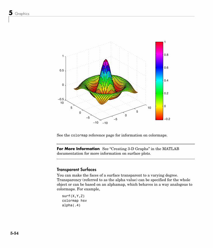
5 Graphics
5-5
See the colormap reference page for information on colormaps.
For More Information See “Creating 3-D Graphs” in the MATLAB documentation for more information on surface plots.
Transparent SurfacesYou can make the faces of a surface transparent to a varying degree. Transparency (referred to as the alpha value) can be specified for the whole object or can be based on an alphamap, which behaves in a way analogous to colormaps. For example,
surf(X,Y,Z)colormap hsvalpha(.4)
−0.2
0
0.2
0.4
0.6
0.8
1
−10−5
05
10
−10
−5
0
5
10−0.5
0
0.5
1
4
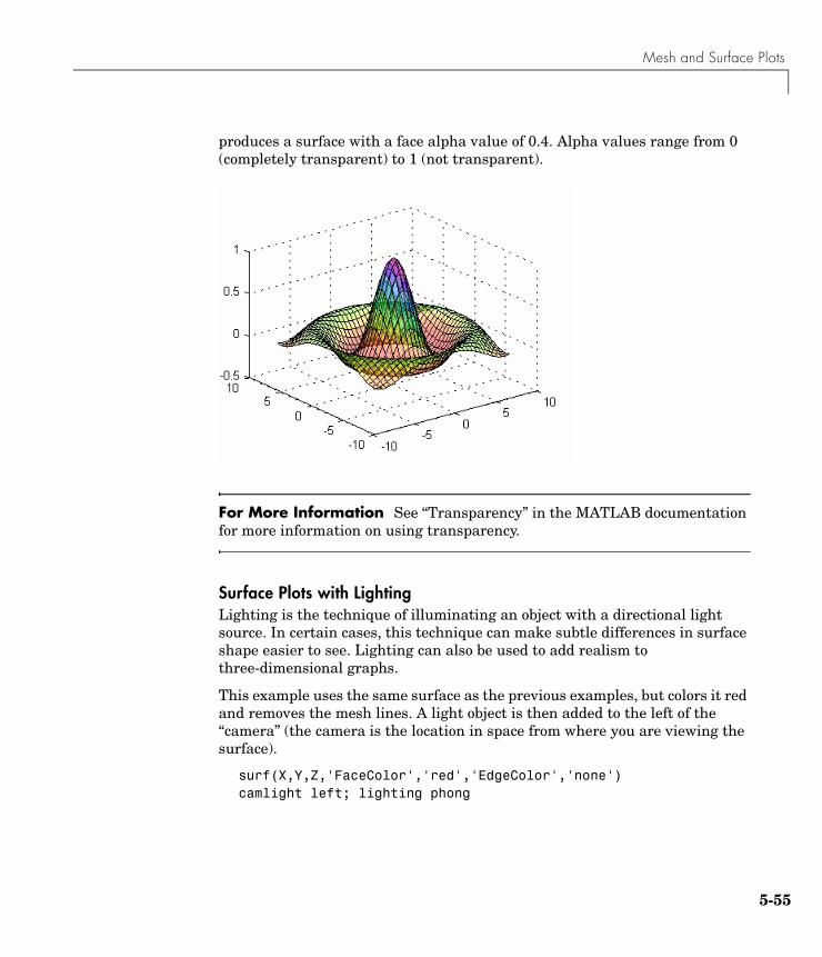
Mesh and Surface Plots
produces a surface with a face alpha value of 0.4. Alpha values range from 0 (completely transparent) to 1 (not transparent).
For More Information See “Transparency” in the MATLAB documentation for more information on using transparency.
Surface Plots with LightingLighting is the technique of illuminating an object with a directional light source. In certain cases, this technique can make subtle differences in surface shape easier to see. Lighting can also be used to add realism to three-dimensional graphs.
This example uses the same surface as the previous examples, but colors it red and removes the mesh lines. A light object is then added to the left of the “camera” (the camera is the location in space from where you are viewing the surface).
surf(X,Y,Z,'FaceColor','red','EdgeColor','none')camlight left; lighting phong
5-55
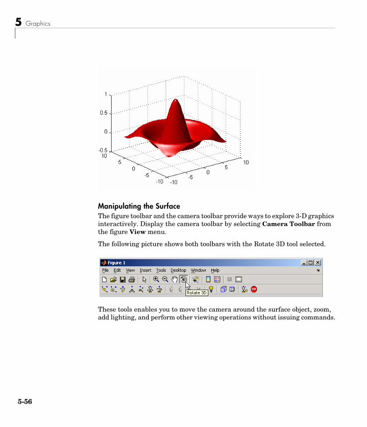
5 Graphics
5-5
Manipulating the SurfaceThe figure toolbar and the camera toolbar provide ways to explore 3-D graphics interactively. Display the camera toolbar by selecting Camera Toolbar from the figure View menu.
The following picture shows both toolbars with the Rotate 3D tool selected.
These tools enables you to move the camera around the surface object, zoom, add lighting, and perform other viewing operations without issuing commands.
6
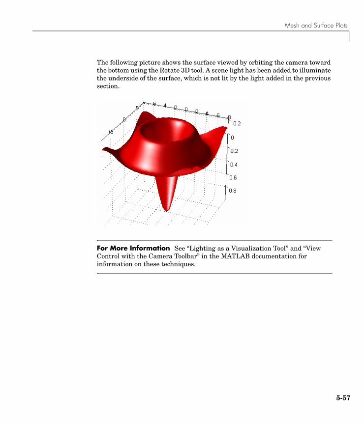
Mesh and Surface Plots
The following picture shows the surface viewed by orbiting the camera toward the bottom using the Rotate 3D tool. A scene light has been added to illuminate the underside of the surface, which is not lit by the light added in the previous section.
For More Information See “Lighting as a Visualization Tool” and “View Control with the Camera Toolbar” in the MATLAB documentation for information on these techniques.
5-57
5 Graphics
5-5
ImagesTwo-dimensional arrays can be displayed as images, where the array elements determine brightness or color of the images. For example, the statements
load durerwhosName Size Bytes Class
X 648x509 2638656 double array caption 2x28 112 char array map 128x3 3072 double array
load the file durer.mat, adding three variables to the workspace. The matrix X is a 648-by-509 matrix and map is a 128-by-3 matrix that is the colormap for this image.
MAT-files, such as durer.mat, are binary files that can be created on one platform and later read by MATLAB on a different platform.
The elements of X are integers between 1 and 128, which serve as indices into the colormap, map. Then
image(X)colormap(map)axis image
reproduces Dürer’s etching shown at the beginning of this book. A high-resolution scan of the magic square in the upper right corner is available in another file. Type
load detail
and then use the up arrow key on your keyboard to reexecute the image, colormap, and axis commands. The statement
colormap(hot)
adds some twentieth century colorization to the sixteenth century etching. The function hot generates a colormap containing shades of reds, oranges, and yellows. Typically a given image matrix has a specific colormap associated with it. See the colormap reference page for a list of other predefined colormaps.
8
Images
Reading and Writing ImagesYou can read standard image files (TIFF, JPEG, BMP, etc.) into MATLAB using the imread function. The type of data returned by imread depends on the type of image you are reading.
You can write MATLAB data to a variety of standard image formats using the imwrite function. See the reference pages for these functions for more information and examples.
For More Information See “Displaying Bit-Mapped Images” in the MATLAB documentation for information on the image processing capabilities of MATLAB.
5-59
5 Graphics
5-6
Printing GraphicsYou can print a MATLAB figure directly on a printer connected to your computer or you can export the figure to one of the standard graphics file formats supported by MATLAB. There are two ways to print and export figures:
• Use the Print or Export Setup options under the File menu
• Use the print command to print or export the figure
See “Preparing Graphs for Presentation” on page 5-29 for an example.
Printing from the MenuThere are four menu options under the File menu that pertain to printing:
• The Page Setup option displays a dialog box that enables you to adjust characteristics of the figure on the printed page.
• The Print Setup option displays a dialog box that sets printing defaults, but does not actually print the figure.
• The Print Preview option enables you to view the figure the way it will look on the printed page.
• The Print option displays a dialog box that lets you select standard printing options and print the figure.
Generally, use Print Preview to determine whether the printed output is what you want. If not, use the Page Setup dialog box to change the output settings. Select the Page Setup dialog box Help button to display information on how to set up the page.
Exporting Figure to Graphics FilesThe Export Setup option in the File menu enables you to set a variety of figure characteristics, such as size and font type, as well as apply predefined templates to achieve standard-looking graphics files. After setup, you can export the figure to a number of standard graphics file formats.
0
Printing Graphics
Using the Print CommandThe print command provides more flexibility in the type of output sent to the printer and allows you to control printing from M-files. The result can be sent directly to your default printer or stored in a specified file. A wide variety of output formats, including TIFF, JPEG, and PostScript, is available.
For example, this statement saves the contents of the current figure window as color Encapsulated Level 2 PostScript in the file called magicsquare.eps. It also includes a TIFF preview, which enables most word processors to display the picture.
print -depsc2 -tiff magicsquare.eps
To save the same figure as a TIFF file with a resolution of 200 dpi, use the command
print -dtiff -r200 magicsquare.tiff
If you type print on the command line,
MATLAB prints the current figure on your default printer.
For More Information See the print reference page and “Printing and Exporting” in the MATLAB documentation for more information on printing.
5-61
5 Graphics
5-6
Handle GraphicsHandle Graphics® refers to a system of graphics objects that MATLAB uses to implement graphing and visualization functions. Each object created has a fixed set of properties. You can use these properties to control the behavior and appearance of your graph.
When you call a plotting function, MATLAB creates the graph using various graphics objects, such as a figure window, axes, lines, text, and so on. MATLAB enables you to query the value of each property and set the values of most properties.
For example, the following statement creates a figure with a white background color and without displaying the figure toolbar.
figure('Color','white','Toolbar','none')
Using the HandleWhenever MATLAB creates a graphics object, it assigns an identifier (called a handle) to the object. You can use this handle to access the object’s properties with the set and get functions. For example, the following statements create a graph and return a handle to a lineseries object in h.
x = 1:10;y = x.^3;h = plot(x,y);
You can use the handle h to set the properties of the lineseries object. For example, you can set its Color property:
set(h,'Color','red')
You can also specify properties when you call the plotting function.
h = plot(x,y,'Color','red');
When you query the lineseries properties,
get(h,'LineWidth')
MATLAB returns the answer:
ans =0.5000
2
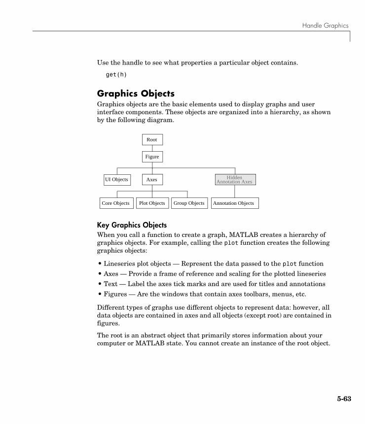
Handle Graphics
Use the handle to see what properties a particular object contains.
get(h)
Graphics ObjectsGraphics objects are the basic elements used to display graphs and user interface components. These objects are organized into a hierarchy, as shown by the following diagram.
Key Graphics ObjectsWhen you call a function to create a graph, MATLAB creates a hierarchy of graphics objects. For example, calling the plot function creates the following graphics objects:
• Lineseries plot objects — Represent the data passed to the plot function
• Axes — Provide a frame of reference and scaling for the plotted lineseries
• Text — Label the axes tick marks and are used for titles and annotations
• Figures — Are the windows that contain axes toolbars, menus, etc.
Different types of graphs use different objects to represent data: however, all data objects are contained in axes and all objects (except root) are contained in figures.
The root is an abstract object that primarily stores information about your computer or MATLAB state. You cannot create an instance of the root object.
Axes
Core Objects
Figure
Root
Annotation ObjectsPlot Objects
Annotation AxesHidden
Group Objects
UI Objects
5-63
5 Graphics
5-6
For More Information See “Handle Graphics Objects” in the MATLAB documentation for information on graphics objects.
User interface objects are used to create graphical user interfaces (GUIs). These objects include components like push buttons, editable text boxes, and list boxes.
For More Information See “Creating Graphical User Interfaces” in the MATLAB documentation for more information on user interface objects.
Creating ObjectsPlotting functions (like plot and surf) call the appropriate low-level function to draw their respective graph. For information about an object’s properties, see the Handle Graphics Property Browser in the MATLAB online documentation.
Commands for Working with ObjectsThis table lists commands commonly used when working with objects.
Function Purpose
allchild Find all children of specified objects
ancestor Find ancestor of graphics object
copyobj Copy graphics object
delete Delete an object
findall Find all graphics objects (including hidden handles)
findobj Find the handles of objects having specified property values
gca Return the handle of the current axes
4
Handle Graphics
Setting Object PropertiesAll object properties have default values. However, you might find it useful to change the settings of some properties to customize your graph. There are two ways to set object properties:
• Specify values for properties when you create the object.
• Set the property value on an object that already exists.
Setting Properties from Plotting CommandsYou can specify object property value pairs as arguments to many plotting functions, such as plot, mesh, and surf.
For example, plotting commands that create lineseries or surfaceplot objects enable you to specify property name/property value pairs as arguments. The command
surf(x,y,z,'FaceColor','interp',...'FaceLighting','gouraud')
plots the data in the variables x, y, and z using a surfaceplot object with interpolated face color and employing the Gouraud face light technique. You can set any of the object’s properties this way.
Setting Properties of Existing ObjectsTo modify the property values of existing objects, you can use the set command or the Property Editor. This section describes how to use the set command. See “Using the Property Editor” on page 5-17 for more information.
gcf Return the handle of the current figure
gco Return the handle of the current object
get Query the values of an object’s properties
ishandle True if value is valid object handle
set Set the values of an object’s properties
Function Purpose
5-65
5 Graphics
5-6
Most plotting functions return the handles of the objects that they create so you can modify the objects using the set command. For example, these statements plot a five-by-five matrix (creating five lineseries, one per column) and then set the Marker property to a square and the MarkerFaceColor property to green.
h = plot(magic(5));set(h,'Marker','s','MarkerFaceColor','g')
In this case, h is a vector containing five handles, one for each of the five lineseries in the graph. The set statement sets the Marker and MarkerFaceColor properties of all lineseries to the same values.
Setting Multiple Property ValuesIf you want to set the properties of each lineseries to a different value, you can use cell arrays to store all the data and pass it to the set command. For example, create a plot and save the lineseries handles.
h = plot(magic(5));
Suppose you want to add different markers to each lineseries and color the marker’s face color the same color as the lineseries. You need to define two cell arrays — one containing the property names and the other containing the desired values of the properties.
The prop_name cell array contains two elements.
prop_name(1) = {'Marker'};prop_name(2) = {'MarkerFaceColor'};
The prop_values cell array contains 10 values: five values for the Marker property and five values for the MarkerFaceColor property. Notice that prop_values is a two-dimensional cell array. The first dimension indicates which handle in h the values apply to and the second dimension indicates which property the value is assigned to.
prop_values(1,1) = {'s'};prop_values(1,2) = {get(h(1),'Color')};prop_values(2,1) = {'d'};prop_values(2,2) = {get(h(2),'Color')};prop_values(3,1) = {'o'};prop_values(3,2) = {get(h(3),'Color')};prop_values(4,1) = {'p'};prop_values(4,2) = {get(h(4),'Color')};
6
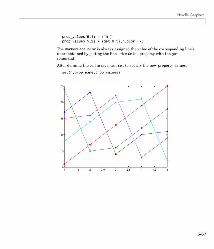
Handle Graphics
prop_values(5,1) = {'h'};prop_values(5,2) = {get(h(5),'Color')};
The MarkerFaceColor is always assigned the value of the corresponding line’s color (obtained by getting the lineseries Color property with the get command).
After defining the cell arrays, call set to specify the new property values.
set(h,prop_name,prop_values)
1 1.5 2 2.5 3 3.5 4 4.5 50
5
10
15
20
25
5-67
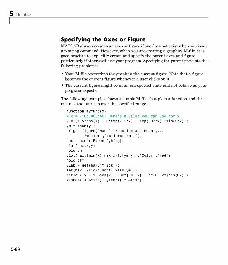
5 Graphics
5-6
Specifying the Axes or FigureMATLAB always creates an axes or figure if one does not exist when you issue a plotting command. However, when you are creating a graphics M-file, it is good practice to explicitly create and specify the parent axes and figure, particularly if others will use your program. Specifying the parent prevents the following problems:
• Your M-file overwrites the graph in the current figure. Note that a figure becomes the current figure whenever a user clicks on it.
• The current figure might be in an unexpected state and not behave as your program expects.
The following examples shows a simple M-file that plots a function and the mean of the function over the specified range.
function myfunc(x)% x = -10:.005:40; Here's a value you can use for xy = [1.5*cos(x) + 6*exp(-.1*x) + exp(.07*x).*sin(3*x)];ym = mean(y);hfig = figure('Name','Function and Mean',...
'Pointer','fullcrosshair');hax = axes('Parent',hfig);plot(hax,x,y)hold onplot(hax,[min(x) max(x)],[ym ym],'Color','red')hold offylab = get(hax,'YTick');set(hax,'YTick',sort([ylab ym]))title ('y = 1.5cos(x) + 6e^{-0.1x} + e^{0.07x}sin(3x)')xlabel('X Axis'); ylabel('Y Axis')
8
Handle Graphics
Finding the Handles of Existing ObjectsThe findobj function enables you to obtain the handles of graphics objects by searching for objects with particular property values. With findobj you can specify the values of any combination of properties, which makes it easy to pick one object out of many. findobj also recognizes regular expressions (regexp).
For example, you might want to find the blue line with square marker having blue face color.You can also specify which figures or axes to search, if there are more than one. The following sections provide examples illustrating how to use findobj.
Finding All Objects of a Certain TypeBecause all objects have a Type property that identifies the type of object, you can find the handles of all occurrences of a particular type of object. For example,
h = findobj('Type','patch');
finds the handles of all patch objects.
−10 −5 0 5 10 15 20 25 30 35 40−20
−15
−10
−5
0
3.1596
5
10
15
20y = 1.5cos(x) + 6e−0.1x + e0.07xsin(3x)
X Axis
Y A
xis
5-69
5 Graphics
5-7
Finding Objects with a Particular PropertyYou can specify multiple properties to narrow the search. For example,
h = findobj('Type','line','Color','r','LineStyle',':');
finds the handles of all red dotted lines.
Limiting the Scope of the SearchYou can specify the starting point in the object hierarchy by passing the handle of the starting figure or axes as the first argument. For example,
h = findobj(gca,'Type','text','String','\pi/2');
finds the string π/2 only within the current axes.
Using findobj as an ArgumentBecause findobj returns the handles it finds, you can use it in place of the handle argument. For example,
set(findobj('Type','line','Color','red'),'LineStyle',':')
finds all red lines and sets their line style to dotted.
0
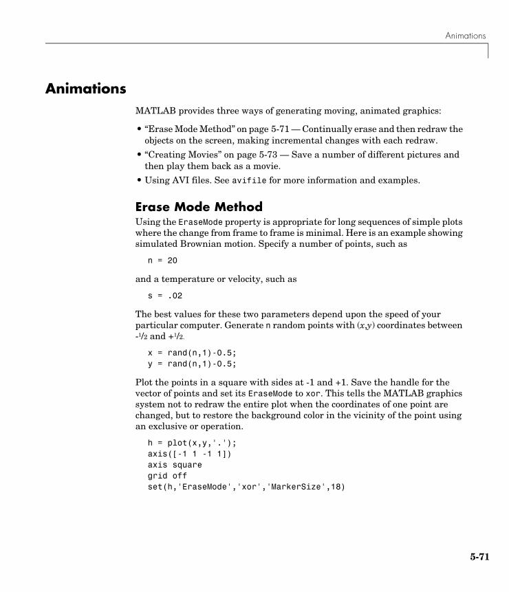
Animations
AnimationsMATLAB provides three ways of generating moving, animated graphics:
• “Erase Mode Method” on page 5-71 — Continually erase and then redraw the objects on the screen, making incremental changes with each redraw.
• “Creating Movies” on page 5-73 — Save a number of different pictures and then play them back as a movie.
• Using AVI files. See avifile for more information and examples.
Erase Mode MethodUsing the EraseMode property is appropriate for long sequences of simple plots where the change from frame to frame is minimal. Here is an example showing simulated Brownian motion. Specify a number of points, such as
n = 20
and a temperature or velocity, such as
s = .02
The best values for these two parameters depend upon the speed of your particular computer. Generate n random points with (x,y) coordinates between -1/2 and +1/2.
x = rand(n,1)-0.5;y = rand(n,1)-0.5;
Plot the points in a square with sides at -1 and +1. Save the handle for the vector of points and set its EraseMode to xor. This tells the MATLAB graphics system not to redraw the entire plot when the coordinates of one point are changed, but to restore the background color in the vicinity of the point using an exclusive or operation.
h = plot(x,y,'.');axis([-1 1 -1 1])axis squaregrid offset(h,'EraseMode','xor','MarkerSize',18)
5-71
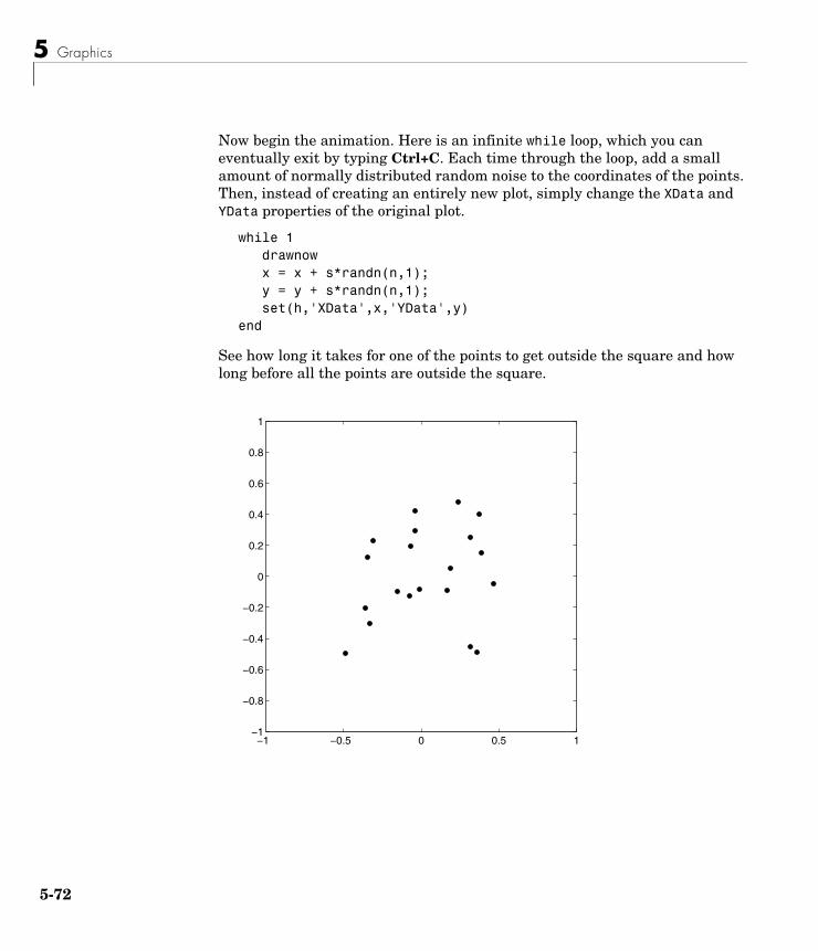
5 Graphics
5-7
Now begin the animation. Here is an infinite while loop, which you can eventually exit by typing Ctrl+C. Each time through the loop, add a small amount of normally distributed random noise to the coordinates of the points. Then, instead of creating an entirely new plot, simply change the XData and YData properties of the original plot.
while 1 drawnow x = x + s*randn(n,1); y = y + s*randn(n,1); set(h,'XData',x,'YData',y)end
See how long it takes for one of the points to get outside the square and how long before all the points are outside the square.
−1 −0.5 0 0.5 1−1
−0.8
−0.6
−0.4
−0.2
0
0.2
0.4
0.6
0.8
1
2
Animations
Creating MoviesIf you increase the number of points in the Brownian motion example to n = 300 and s = .02, the motion is no longer very fluid; it takes too much time to draw each time step. It becomes more effective to save a predetermined number of frames as bitmaps and to play them back as a movie.
First, decide on the number of frames,
nframes = 50;
Next, set up the first plot as before, except using the default EraseMode (normal).
x = rand(n,1)-0.5;y = rand(n,1)-0.5;h = plot(x,y,'.');set(h,'MarkerSize',18);axis([-1 1 -1 1])axis squaregrid off
Generate the movie and use getframe to capture each frame.
for k = 1:nframes x = x + s*randn(n,1); y = y + s*randn(n,1); set(h,'XData',x,'YData',y) M(k) = getframe;end
Finally, play the movie 30 times.
movie(M,30)
5-73

5 Graphics
5-7
4
6
Programming
This chapter introduces programming constructs, multidimensional arrays and other data structures, and MATLAB functions.
Flow Control (p. 6-2) Use flow control constructs including if, switch and case, for, while, continue, and break.
Other Data Structures (p. 6-9) Work with multidimensional arrays, cell arrays, character and text data, and structures.
Scripts and Functions (p. 6-19) Write scripts and functions, use global variables, pass string arguments to functions, use eval to evaluate text expressions, vectorize code, preallocate arrays, reference functions using handles, and use functions that operate on functions.
6 Programming
6-2
Flow ControlMATLAB has several flow control constructs:
• “if” on page 6-2
• “switch and case” on page 6-4
• “for” on page 6-5
• “while” on page 6-6
• “continue” on page 6-6
• “break” on page 6-7
• “try - catch” on page 6-8
• “return” on page 6-8
ifThe if statement evaluates a logical expression and executes a group of statements when the expression is true. The optional elseif and else keywords provide for the execution of alternate groups of statements. An end keyword, which matches the if, terminates the last group of statements. The groups of statements are delineated by the four keywords — no braces or brackets are involved.
The MATLAB algorithm for generating a magic square of order n involves three different cases: when n is odd, when n is even but not divisible by 4, or when n is divisible by 4. This is described by
if rem(n,2) ~= 0 M = odd_magic(n)elseif rem(n,4) ~= 0 M = single_even_magic(n)else M = double_even_magic(n)end
In this example, the three cases are mutually exclusive, but if they weren’t, the first true condition would be executed.
Flow Control
It is important to understand how relational operators and if statements work with matrices. When you want to check for equality between two variables, you might use
if A == B, ...
This is valid MATLAB code, and does what you expect when A and B are scalars. But when A and B are matrices, A == B does not test if they are equal, it tests where they are equal; the result is another matrix of 0’s and 1’s showing element-by-element equality. (In fact, if A and B are not the same size, then A == B is an error.)
A = magic(4); B = A; B(1,1) = 0;
A == Bans = 0 1 1 1 1 1 1 1 1 1 1 1 1 1 1 1
The proper way to check for equality between two variables is to use the isequal function,
if isequal(A,B), ...
isequal returns a scalar logical value of 1 (representing true) or 0 (false), instead of a matrix, as the expression to be evaluated by the if function. Using the A and B matrices from above, you get
isequal(A, B)ans = 0
Here is another example to emphasize this point. If A and B are scalars, the following program will never reach the “unexpected situation”. But for most pairs of matrices, including our magic squares with interchanged columns, none of the matrix conditions A > B, A < B, or A == B is true for all elements and so the else clause is executed.
6-3
6 Programming
6-4
if A > B 'greater'elseif A < B 'less'elseif A == B 'equal'else error('Unexpected situation')end
Several functions are helpful for reducing the results of matrix comparisons to scalar conditions for use with if, including
isequalisemptyallany
switch and caseThe switch statement executes groups of statements based on the value of a variable or expression. The keywords case and otherwise delineate the groups. Only the first matching case is executed. There must always be an end to match the switch.
The logic of the magic squares algorithm can also be described by
switch (rem(n,4)==0) + (rem(n,2)==0) case 0 M = odd_magic(n) case 1 M = single_even_magic(n) case 2 M = double_even_magic(n) otherwise error('This is impossible') end
Flow Control
Note Unlike the C language switch statement, MATLAB switch does not fall through. If the first case statement is true, the other case statements do not execute. So, break statements are not required.
forThe for loop repeats a group of statements a fixed, predetermined number of times. A matching end delineates the statements.
for n = 3:32 r(n) = rank(magic(n));endr
The semicolon terminating the inner statement suppresses repeated printing, and the r after the loop displays the final result.
6-5
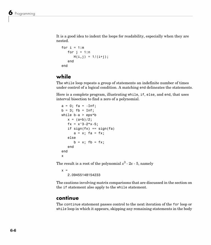
6 Programming
6-6
It is a good idea to indent the loops for readability, especially when they are nested.
for i = 1:m for j = 1:n H(i,j) = 1/(i+j); endend
whileThe while loop repeats a group of statements an indefinite number of times under control of a logical condition. A matching end delineates the statements.
Here is a complete program, illustrating while, if, else, and end, that uses interval bisection to find a zero of a polynomial.
a = 0; fa = -Inf;b = 3; fb = Inf;while b-a > eps*b x = (a+b)/2; fx = x^3-2*x-5; if sign(fx) == sign(fa) a = x; fa = fx; else b = x; fb = fx; endendx
The result is a root of the polynomial x3 - 2x - 5, namely
x = 2.09455148154233
The cautions involving matrix comparisons that are discussed in the section on the if statement also apply to the while statement.
continueThe continue statement passes control to the next iteration of the for loop or while loop in which it appears, skipping any remaining statements in the body
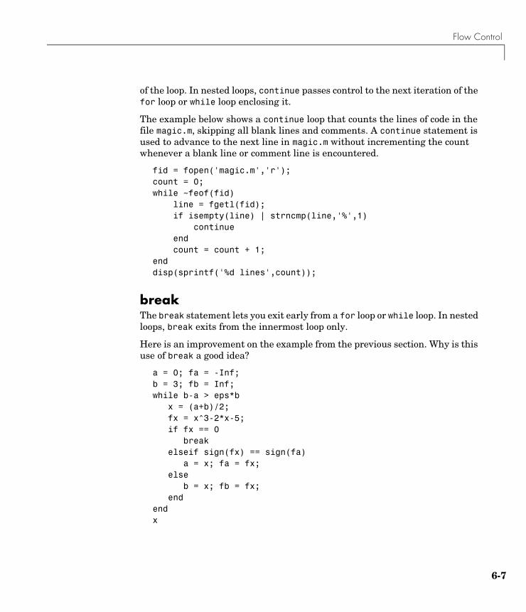
Flow Control
of the loop. In nested loops, continue passes control to the next iteration of the for loop or while loop enclosing it.
The example below shows a continue loop that counts the lines of code in the file magic.m, skipping all blank lines and comments. A continue statement is used to advance to the next line in magic.m without incrementing the count whenever a blank line or comment line is encountered.
fid = fopen('magic.m','r');count = 0;while ~feof(fid) line = fgetl(fid); if isempty(line) | strncmp(line,'%',1) continue end count = count + 1;enddisp(sprintf('%d lines',count));
breakThe break statement lets you exit early from a for loop or while loop. In nested loops, break exits from the innermost loop only.
Here is an improvement on the example from the previous section. Why is this use of break a good idea?
a = 0; fa = -Inf;b = 3; fb = Inf;while b-a > eps*b x = (a+b)/2; fx = x^3-2*x-5; if fx == 0 break elseif sign(fx) == sign(fa) a = x; fa = fx; else b = x; fb = fx; endendx
6-7
6 Programming
6-8
try - catchThe general form of a try-catch statement sequence is
try statement ... statementcatch statement ... statementend
In this sequence the statements between try and catch are executed until an error occurs. The statements between catch and end are then executed. Use lasterr to see the cause of the error. If an error occurs between catch and end, MATLAB terminates execution unless another try-catch sequence has been established.
returnreturn terminates the current sequence of commands and returns control to the invoking function or to the keyboard. return is also used to terminate keyboard mode. A called function normally transfers control to the function that invoked it when it reaches the end of the function. You can insert a return statement within the called function to force an early termination and to transfer control to the invoking function.
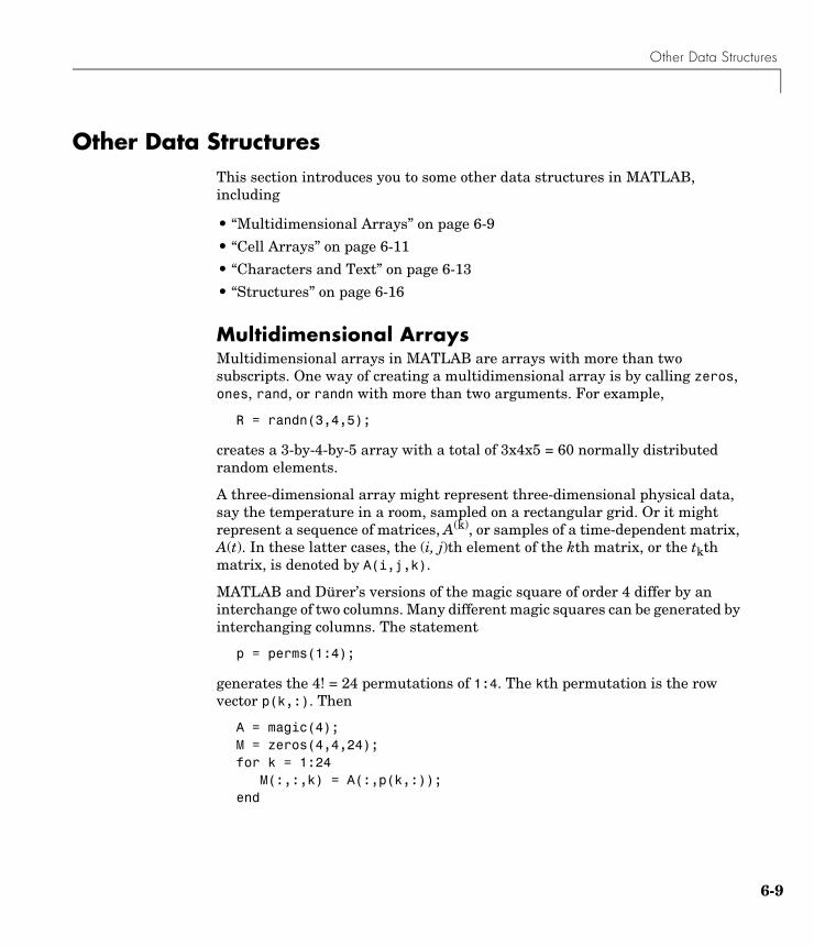
Other Data Structures
Other Data StructuresThis section introduces you to some other data structures in MATLAB, including
• “Multidimensional Arrays” on page 6-9
• “Cell Arrays” on page 6-11
• “Characters and Text” on page 6-13
• “Structures” on page 6-16
Multidimensional ArraysMultidimensional arrays in MATLAB are arrays with more than two subscripts. One way of creating a multidimensional array is by calling zeros, ones, rand, or randn with more than two arguments. For example,
R = randn(3,4,5);
creates a 3-by-4-by-5 array with a total of 3x4x5 = 60 normally distributed random elements.
A three-dimensional array might represent three-dimensional physical data, say the temperature in a room, sampled on a rectangular grid. Or it might represent a sequence of matrices, A(k), or samples of a time-dependent matrix, A(t). In these latter cases, the (i, j)th element of the kth matrix, or the tkth matrix, is denoted by A(i,j,k).
MATLAB and Dürer’s versions of the magic square of order 4 differ by an interchange of two columns. Many different magic squares can be generated by interchanging columns. The statement
p = perms(1:4);
generates the 4! = 24 permutations of 1:4. The kth permutation is the row vector p(k,:). Then
A = magic(4);M = zeros(4,4,24);for k = 1:24 M(:,:,k) = A(:,p(k,:));end
6-9
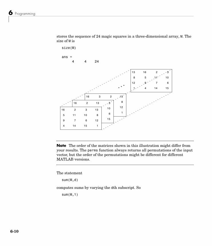
6 Programming
6-1
stores the sequence of 24 magic squares in a three-dimensional array, M. The size of M is
size(M)
ans = 4 4 24
Note The order of the matrices shown in this illustration might differ from your results. The perms function always returns all permutations of the input vector, but the order of the permutations might be different for different MATLAB versions.
The statement
sum(M,d)
computes sums by varying the dth subscript. So
sum(M,1)
16 3 2 13
8 11 10 8
12 7 6 12
1 14 15 1
16 2 13 3
10 8 11 10
6 12 7 6
15 1 14 15
13 16 2 3
8 5 11 10
12 9 7 6
1 4 14 15
16 2 3 13
5 11 10 8
9 7 6 12
4 14 15 1
...
0
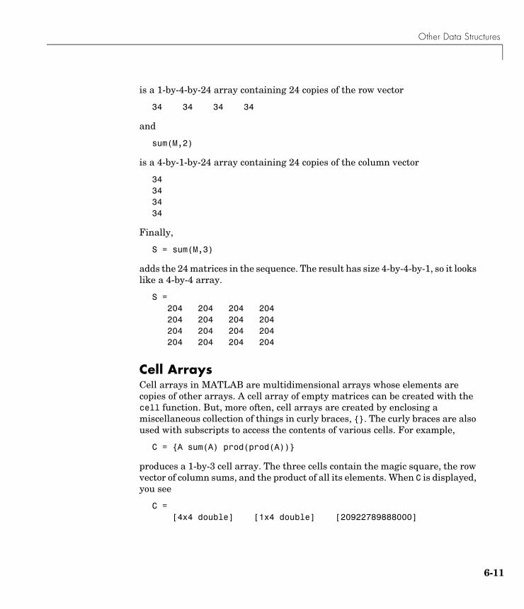
Other Data Structures
is a 1-by-4-by-24 array containing 24 copies of the row vector
34 34 34 34
and
sum(M,2)
is a 4-by-1-by-24 array containing 24 copies of the column vector
34 34 34 34
Finally,
S = sum(M,3)
adds the 24 matrices in the sequence. The result has size 4-by-4-by-1, so it looks like a 4-by-4 array.
S = 204 204 204 204 204 204 204 204 204 204 204 204 204 204 204 204
Cell ArraysCell arrays in MATLAB are multidimensional arrays whose elements are copies of other arrays. A cell array of empty matrices can be created with the cell function. But, more often, cell arrays are created by enclosing a miscellaneous collection of things in curly braces, {}. The curly braces are also used with subscripts to access the contents of various cells. For example,
C = {A sum(A) prod(prod(A))}
produces a 1-by-3 cell array. The three cells contain the magic square, the row vector of column sums, and the product of all its elements. When C is displayed, you see
C = [4x4 double] [1x4 double] [20922789888000]
6-11
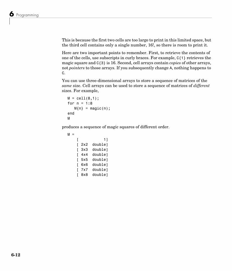
6 Programming
6-1
This is because the first two cells are too large to print in this limited space, but the third cell contains only a single number, 16!, so there is room to print it.
Here are two important points to remember. First, to retrieve the contents of one of the cells, use subscripts in curly braces. For example, C{1} retrieves the magic square and C{3} is 16. Second, cell arrays contain copies of other arrays, not pointers to those arrays. If you subsequently change A, nothing happens to C.
You can use three-dimensional arrays to store a sequence of matrices of the same size. Cell arrays can be used to store a sequence of matrices of different sizes. For example,
M = cell(8,1);for n = 1:8 M{n} = magic(n);endM
produces a sequence of magic squares of different order.
M = [ 1] [ 2x2 double] [ 3x3 double] [ 4x4 double] [ 5x5 double] [ 6x6 double] [ 7x7 double] [ 8x8 double]
2
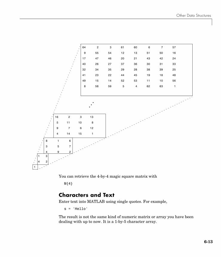
Other Data Structures
You can retrieve the 4-by-4 magic square matrix with
M{4}
Characters and TextEnter text into MATLAB using single quotes. For example,
s = 'Hello'
The result is not the same kind of numeric matrix or array you have been dealing with up to now. It is a 1-by-5 character array.
16 2 3 13
5 11 10 8
9 7 6 12
4 14 15 1
...
64 2 3 61 60 6 7 57
9 55 54 12 13 51 50 16
17 47 46 20 21 43 42 24
40 26 27 37 36 30 31 33
32 34 35 29 28 38 39 25
41 23 22 44 45 19 18 48
49 15 14 52 53 11 10 56
8 58 59 5 4 62 63 1
1 3
4 2
8 1 6
3 5 7
4 9 2
1
6-13
6 Programming
6-1
Internally, the characters are stored as numbers, but not in floating-point format. The statement
a = double(s)
converts the character array to a numeric matrix containing floating-point representations of the ASCII codes for each character. The result is
a = 72 101 108 108 111
The statement
s = char(a)
reverses the conversion.
Converting numbers to characters makes it possible to investigate the various fonts available on your computer. The printable characters in the basic ASCII character set are represented by the integers 32:127. (The integers less than 32 represent nonprintable control characters.) These integers are arranged in an appropriate 6-by-16 array with
F = reshape(32:127,16,6)';
The printable characters in the extended ASCII character set are represented by F+128. When these integers are interpreted as characters, the result depends on the font currently being used. Type the statements
char(F)char(F+128)
and then vary the font being used for the Command Window. Select Preferences from the File menu to change the font. If you include tabs in lines of code, use a fixed-width font, such as Monospaced, to align the tab positions on different lines.
Concatenation with square brackets joins text variables together into larger strings. The statement
h = [s, ' world']
joins the strings horizontally and produces
h = Hello world
4
Other Data Structures
The statement
v = [s; 'world']
joins the strings vertically and produces
v = Hello world
Note that a blank has to be inserted before the 'w' in h and that both words in v have to have the same length. The resulting arrays are both character arrays; h is 1-by-11 and v is 2-by-5.
To manipulate a body of text containing lines of different lengths, you have two choices — a padded character array or a cell array of strings. When creating a character array, you must make each row of the array the same length. (Pad the ends of the shorter rows with spaces.) The char function does this padding for you. For example,
S = char('A','rolling','stone','gathers','momentum.')
produces a 5-by-9 character array.
S =A rolling stone gathers momentum.
Alternatively, you can store the text in a cell array. For example,
C = {'A';'rolling';'stone';'gathers';'momentum.'}
creates a 5-by-1 cell array that requires no padding because each row of the array can have a different length.
C = 'A' 'rolling' 'stone' 'gathers' 'momentum.'
6-15
6 Programming
6-1
You can convert a padded character array to a cell array of strings with
C = cellstr(S)
and reverse the process with
S = char(C)
StructuresStructures are multidimensional MATLAB arrays with elements accessed by textual field designators. For example,
S.name = 'Ed Plum';S.score = 83;S.grade = 'B+'
creates a scalar structure with three fields.
S = name: 'Ed Plum' score: 83 grade: 'B+'
Like everything else in MATLAB, structures are arrays, so you can insert additional elements. In this case, each element of the array is a structure with several fields. The fields can be added one at a time,
S(2).name = 'Toni Miller';S(2).score = 91;S(2).grade = 'A-';
or an entire element can be added with a single statement.
S(3) = struct('name','Jerry Garcia',... 'score',70,'grade','C')
Now the structure is large enough that only a summary is printed.
S = 1x3 struct array with fields: name score grade
6
Other Data Structures
There are several ways to reassemble the various fields into other MATLAB arrays. They are all based on the notation of a comma-separated list. If you type
S.score
it is the same as typing
S(1).score, S(2).score, S(3).score
This is a comma-separated list. Without any other punctuation, it is not very useful. It assigns the three scores, one at a time, to the default variable ans and dutifully prints out the result of each assignment. But when you enclose the expression in square brackets,
[S.score]
it is the same as
[S(1).score, S(2).score, S(3).score]
which produces a numeric row vector containing all the scores.
ans = 83 91 70
Similarly, typing
S.name
just assigns the names, one at a time, to ans. But enclosing the expression in curly braces,
{S.name}
creates a 1-by-3 cell array containing the three names.
ans = 'Ed Plum' 'Toni Miller' 'Jerry Garcia'
And
char(S.name)
6-17
6 Programming
6-1
calls the char function with three arguments to create a character array from the name fields,
ans =Ed Plum Toni MillerJerry Garcia
Dynamic Field NamesThe most common way to access the data in a structure is by specifying the name of the field that you want to reference. Another means of accessing structure data is to use dynamic field names. These names express the field as a variable expression that MATLAB evaluates at run-time. The dot-parentheses syntax shown here makes expression a dynamic field name.
structName.(expression)
Index into this field using the standard MATLAB indexing syntax. For example, to evaluate expression into a field name and obtain the values of that field at columns 1 through 25 of row 7, use
structName.(expression)(7,1:25)
Dynamic Field Names Example. The avgscore function shown below computes an average test score, retrieving information from the testscores structure using dynamic field names:
function avg = avgscore(testscores, student, first, last)for k = first:last scores(k) = testscores.(student).week(k);endavg = sum(scores)/(last - first + 1);
You can run this function using different values for the dynamic field student.
avgscore(testscores, 'Ann Lane', 1, 20)ans = 83.5000
avgscore(testscores, 'William King', 1, 20)ans = 92.1000
8
Scripts and Functions
Scripts and FunctionsTopics covered in this section are
• “Scripts” on page 6-20
• “Functions” on page 6-21
• “Global Variables” on page 6-25
• “Passing String Arguments to Functions” on page 6-26
• “The eval Function” on page 6-27
• “Function Handles” on page 6-28
• “Function Functions” on page 6-28
• “Vectorization” on page 6-31
• “Preallocation” on page 6-31
MATLAB is a powerful programming language as well as an interactive computational environment. Files that contain code in the MATLAB language are called M-files. You create M-files using a text editor, then use them as you would any other MATLAB function or command.
There are two kinds of M-files:
• Scripts, which do not accept input arguments or return output arguments. They operate on data in the workspace.
• Functions, which can accept input arguments and return output arguments. Internal variables are local to the function.
If you’re a new MATLAB programmer, just create the M-files that you want to try out in the current directory. As you develop more of your own M-files, you will want to organize them into other directories and personal toolboxes that you can add to your MATLAB search path.
If you duplicate function names, MATLAB executes the one that occurs first in the search path.
To view the contents of an M-file, for example, myfunction.m, use
type myfunction
6-19
6 Programming
6-2
ScriptsWhen you invoke a script, MATLAB simply executes the commands found in the file. Scripts can operate on existing data in the workspace, or they can create new data on which to operate. Although scripts do not return output arguments, any variables that they create remain in the workspace, to be used in subsequent computations. In addition, scripts can produce graphical output using functions like plot.
For example, create a file called magicrank.m that contains these MATLAB commands.
% Investigate the rank of magic squaresr = zeros(1,32);for n = 3:32 r(n) = rank(magic(n));endrbar(r)
Typing the statement
magicrank
causes MATLAB to execute the commands, compute the rank of the first 30 magic squares, and plot a bar graph of the result. After execution of the file is complete, the variables n and r remain in the workspace.
0
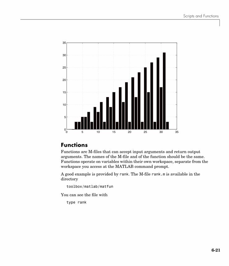
Scripts and Functions
Functions Functions are M-files that can accept input arguments and return output arguments. The names of the M-file and of the function should be the same. Functions operate on variables within their own workspace, separate from the workspace you access at the MATLAB command prompt.
A good example is provided by rank. The M-file rank.m is available in the directory
toolbox/matlab/matfun
You can see the file with
type rank
0 5 10 15 20 25 30 350
5
10
15
20
25
30
35
6-21
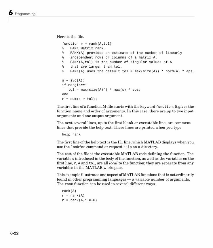
6 Programming
6-2
Here is the file.
function r = rank(A,tol)% RANK Matrix rank.% RANK(A) provides an estimate of the number of linearly% independent rows or columns of a matrix A.% RANK(A,tol) is the number of singular values of A% that are larger than tol.% RANK(A) uses the default tol = max(size(A)) * norm(A) * eps.
s = svd(A);if nargin==1 tol = max(size(A)') * max(s) * eps;endr = sum(s > tol);
The first line of a function M-file starts with the keyword function. It gives the function name and order of arguments. In this case, there are up to two input arguments and one output argument.
The next several lines, up to the first blank or executable line, are comment lines that provide the help text. These lines are printed when you type
help rank
The first line of the help text is the H1 line, which MATLAB displays when you use the lookfor command or request help on a directory.
The rest of the file is the executable MATLAB code defining the function. The variable s introduced in the body of the function, as well as the variables on the first line, r, A and tol, are all local to the function; they are separate from any variables in the MATLAB workspace.
This example illustrates one aspect of MATLAB functions that is not ordinarily found in other programming languages — a variable number of arguments. The rank function can be used in several different ways.
rank(A)r = rank(A)r = rank(A,1.e-6)
2
Scripts and Functions
Many M-files work this way. If no output argument is supplied, the result is stored in ans. If the second input argument is not supplied, the function computes a default value. Within the body of the function, two quantities named nargin and nargout are available which tell you the number of input and output arguments involved in each particular use of the function. The rank function uses nargin, but does not need to use nargout.
Types of FunctionsMATLAB offers several different types of functions to use in your programming.
Anonymous FunctionsAn anonymous function is a simple form of MATLAB function that does not require an M-file. It consists of a single MATLAB expression and any number of input and output arguments. You can define an anonymous function right at the MATLAB command line, or within an M-file function or script. This gives you a quick means of creating simple functions without having to create M-files each time.
The syntax for creating an anonymous function from an expression is
f = @(arglist)expression
The statement below creates an anonymous function that finds the square of a number. When you call this function, MATLAB assigns the value you pass in to variable x, and then uses x in the equation x.^2.
sqr = @(x) x.^2;
To execute the sqr function defined above, type
a = sqr(5)a = 25
Primary and SubfunctionsAll functions that are not anonymous must be defined within an M-file. Each M-file has a required primary function that appears first in the file, and any number of subfunctions that follow the primary. Primary functions have a wider scope than subfunctions. That is, primary functions can be invoked from outside of their M-file (from the MATLAB command line or from functions in
6-23
6 Programming
6-2
other M-files) while subfunctions cannot. Subfunctions are visible only to the primary function and other subfunctions within their own M-file.
The rank function shown in the section on “Functions” on page 6-21 is an example of a primary function.
Private FunctionsA private function is a type of primary M-file function. Its unique characteristic is that it is visible only to a limited group of other functions. This type of function can be useful if you want to limit access to a function, or when you choose not to expose the implementation of a function.
Private functions reside in subdirectories with the special name private. They are visible only to functions in the parent directory. For example, assume the directory newmath is on the MATLAB search path. A subdirectory of newmath called private can contain functions that only the functions in newmath can call.
Because private functions are invisible outside the parent directory, they can use the same names as functions in other directories. This is useful if you want to create your own version of a particular function while retaining the original in another directory. Because MATLAB looks for private functions before standard M-file functions, it will find a private function named test.m before a nonprivate M-file named test.m.
Nested FunctionsYou can define functions within the body of any MATLAB M-file function. These are said to be nested within the outer function. A nested function contains any or all of the components of any other M-file function. In this example, function B is nested in function A.
function x = A(p1, p2)...B(p2) function y = B(p3) ... end...end
4
Scripts and Functions
Like other functions, a nested function has its own workspace where variables used by the function are stored. But it also has access to the workspaces of all functions in which it is nested. So, for example, a variable that has a value assigned to it by the primary function can be read or overwritten by a function nested at any level within the primary. Similarly, a variable that is assigned in a nested function can be read or overwritten by any of the functions containing that function.
Function OverloadingOverloaded functions act the same way as overloaded functions in most computer languages. Overloaded functions are useful when you need to create a function that responds to different types of inputs accordingly. For instance, you might want one of your functions to accept both double-precision and integer input, but to handle each type somewhat differently. You can make this difference invisible to the user by creating two separate functions having the same name, and designating one to handle double types and one to handle integers. When you call the function, MATLAB chooses which M-file to dispatch to based on the type of the input arguments.
Global VariablesIf you want more than one function to share a single copy of a variable, simply declare the variable as global in all the functions. Do the same thing at the command line if you want the base workspace to access the variable. The global declaration must occur before the variable is actually used in a function. Although it is not required, using capital letters for the names of global variables helps distinguish them from other variables. For example, create an M-file called falling.m.
function h = falling(t)global GRAVITYh = 1/2*GRAVITY*t.^2;
Then interactively enter the statements
global GRAVITYGRAVITY = 32;y = falling((0:.1:5)');
6-25
6 Programming
6-2
The two global statements make the value assigned to GRAVITY at the command prompt available inside the function. You can then modify GRAVITY interactively and obtain new solutions without editing any files.
Passing String Arguments to FunctionsYou can write MATLAB functions that accept string arguments without the parentheses and quotes. That is, MATLAB interprets
foo a b c
as
foo('a','b','c')
However, when you use the unquoted form, MATLAB cannot return output arguments. For example,
legend apples oranges
creates a legend on a plot using the strings apples and oranges as labels. If you want the legend command to return its output arguments, then you must use the quoted form.
[legh,objh] = legend('apples','oranges');
In addition, you cannot use the unquoted form if any of the arguments is not a string.
Constructing String Arguments in CodeThe quoted form enables you to construct string arguments within the code. The following example processes multiple data files, August1.dat, August2.dat, and so on. It uses the function int2str, which converts an integer to a character, to build the filename.
for d = 1:31 s = ['August' int2str(d) '.dat']; load(s) % Code to process the contents of the d-th fileend
6
Scripts and Functions
A Cautionary NoteWhile the unquoted syntax is convenient, it can be used incorrectly without causing MATLAB to generate an error. For example, given a matrix A,
A = 0 -6 -1 6 2 -16
-5 20 -10
The eig command returns the eigenvalues of A.
eig(A)ans =-3.0710 -2.4645+17.6008i-2.4645-17.6008i
The following statement is not allowed because A is not a string; however, MATLAB does not generate an error.
eig Aans =
65
MATLAB actually takes the eigenvalue of the ASCII numeric equivalent of the letter A (which is the number 65).
The eval FunctionThe eval function works with text variables to implement a powerful text macro facility. The expression or statement
eval(s)
uses the MATLAB interpreter to evaluate the expression or execute the statement contained in the text string s.
The example of the previous section could also be done with the following code, although this would be somewhat less efficient because it involves the full interpreter, not just a function call.
6-27
6 Programming
6-2
for d = 1:31 s = ['load August' int2str(d) '.dat']; eval(s) % Process the contents of the d-th fileend
Function HandlesYou can create a handle to any MATLAB function and then use that handle as a means of referencing the function. A function handle is typically passed in an argument list to other functions, which can then execute, or evaluate, the function using the handle.
Construct a function handle in MATLAB using the at sign, @, before the function name. The following example creates a function handle for the sin function and assigns it to the variable fhandle.
fhandle = @sin;
You can call a function by means of its handle in the same way that you would call the function using its name. The syntax is
fhandle(arg1, arg2, ...);
The function plot_fhandle, shown below, receives a function handle and data, generates y-axis data using the function handle, and plots it.
function x = plot_fhandle(fhandle, data)plot(data, fhandle(data))
When you call plot_fhandle with a handle to the sin function and the argument shown below, the resulting evaluation produces a sine wave plot.
plot_fhandle(@sin, -pi:0.01:pi)
Function FunctionsA class of functions called “function functions” works with nonlinear functions of a scalar variable. That is, one function works on another function. The function functions include
• Zero finding
• Optimization
8
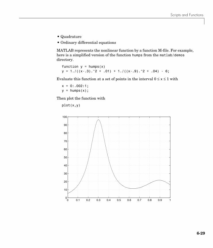
Scripts and Functions
• Quadrature
• Ordinary differential equations
MATLAB represents the nonlinear function by a function M-file. For example, here is a simplified version of the function humps from the matlab/demos directory.
function y = humps(x)y = 1./((x-.3).^2 + .01) + 1./((x-.9).^2 + .04) - 6;
Evaluate this function at a set of points in the interval 0 ≤ x ≤ 1 with
x = 0:.002:1;y = humps(x);
Then plot the function with
plot(x,y)
0 0.1 0.2 0.3 0.4 0.5 0.6 0.7 0.8 0.9 10
10
20
30
40
50
60
70
80
90
100
6-29
6 Programming
6-3
The graph shows that the function has a local minimum near x = 0.6. The function fminsearch finds the minimizer, the value of x where the function takes on this minimum. The first argument to fminsearch is a function handle to the function being minimized and the second argument is a rough guess at the location of the minimum.
p = fminsearch(@humps,.5)p = 0.6370
To evaluate the function at the minimizer,
humps(p)
ans = 11.2528
Numerical analysts use the terms quadrature and integration to distinguish between numerical approximation of definite integrals and numerical integration of ordinary differential equations. MATLAB quadrature routines are quad and quadl. The statement
Q = quadl(@humps,0,1)
computes the area under the curve in the graph and produces
Q = 29.8583
Finally, the graph shows that the function is never zero on this interval. So, if you search for a zero with
z = fzero(@humps,.5)
you will find one outside the interval
z = -0.1316
0
Scripts and Functions
VectorizationOne way to make your MATLAB programs run faster is to vectorize the algorithms you use in constructing the programs. Where other programming languages might use for loops or DO loops, MATLAB can use vector or matrix operations. A simple example involves creating a table of logarithms.
x = .01;for k = 1:1001 y(k) = log10(x); x = x + .01;end
A vectorized version of the same code is
x = .01:.01:10;y = log10(x);
For more complicated code, vectorization options are not always so obvious.
For More Information See “Improving Performance and Memory Usage” in the MATLAB Programming documentation for other techniques that you can use.
Preallocation If you can’t vectorize a piece of code, you can make your for loops go faster by preallocating any vectors or arrays in which output results are stored. For example, this code uses the function zeros to preallocate the vector created in the for loop. This makes the for loop execute significantly faster.
r = zeros(32,1);for n = 1:32 r(n) = rank(magic(n));end
Without the preallocation in the previous example, the MATLAB interpreter enlarges the r vector by one element each time through the loop. Vector preallocation eliminates this step and results in faster execution.
6-31

6 Programming
6-3
2
7
Creating Graphical User InterfacesThis chapter introduces GUIDE, the MATLAB graphical user interface development environment, which is a tool that you can use to create graphical user interfaces.
What Is GUIDE? (p. 7-2) Introduces GUIDE, the MATLAB graphical user interface design environment
Laying Out a GUI (p. 7-3) Briefly describes the GUIDE Layout Editor
Programming a GUI (p. 7-6) Introduces callbacks to define behavior of the GUI components
7 Creating Graphical User Interfaces
7-2
What Is GUIDE?GUIDE, the MATLAB graphical user interface development environment, provides a set of tools for creating graphical user interfaces (GUIs). These tools greatly simplify the process of designing and building GUIs. You can use the GUIDE tools to
• Lay out the GUI.
Using the GUIDE Layout Editor, you can lay out a GUI easily by clicking and dragging GUI components — such as panels, buttons, text fields, sliders, menus, and so on — into the layout area. GUIDE stores the GUI layout in a FIG-file.
• Program the GUI.
GUIDE automatically generates an M-file that controls how the GUI operates. The M-file initializes the GUI and contains a framework for the most commonly used callbacks for each component — the commands that execute when a user clicks a GUI component. Using the M-file editor, you can add code to the callbacks to perform the functions you want.
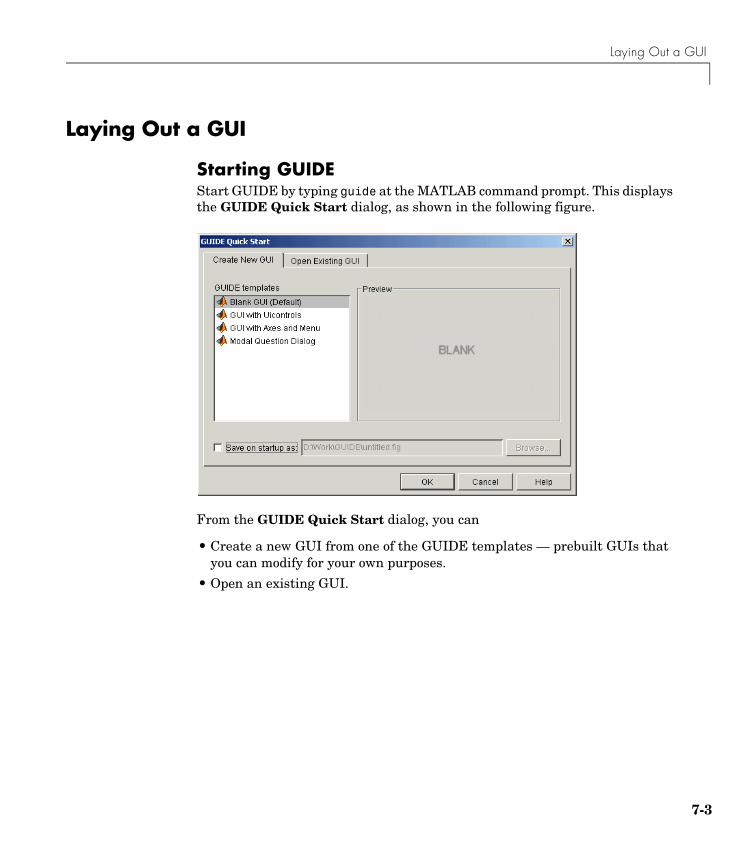
Laying Out a GUI
Laying Out a GUI
Starting GUIDEStart GUIDE by typing guide at the MATLAB command prompt. This displays the GUIDE Quick Start dialog, as shown in the following figure.
From the GUIDE Quick Start dialog, you can
• Create a new GUI from one of the GUIDE templates — prebuilt GUIs that you can modify for your own purposes.
• Open an existing GUI.
7-3
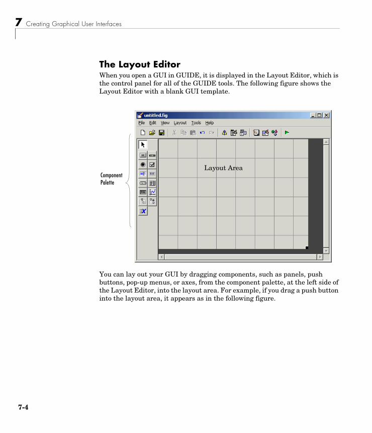
7 Creating Graphical User Interfaces
7-4
The Layout EditorWhen you open a GUI in GUIDE, it is displayed in the Layout Editor, which is the control panel for all of the GUIDE tools. The following figure shows the Layout Editor with a blank GUI template.
You can lay out your GUI by dragging components, such as panels, push buttons, pop-up menus, or axes, from the component palette, at the left side of the Layout Editor, into the layout area. For example, if you drag a push button into the layout area, it appears as in the following figure.
Component Palette
Layout Area
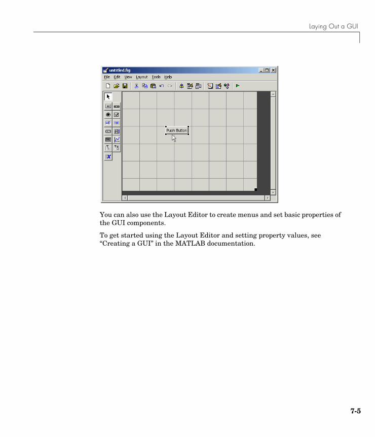
Laying Out a GUI
You can also use the Layout Editor to create menus and set basic properties of the GUI components.
To get started using the Layout Editor and setting property values, see “Creating a GUI” in the MATLAB documentation.
7-5
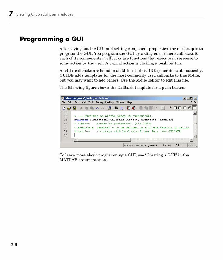
7 Creating Graphical User Interfaces
7-6
Programming a GUIAfter laying out the GUI and setting component properties, the next step is to program the GUI. You program the GUI by coding one or more callbacks for each of its components. Callbacks are functions that execute in response to some action by the user. A typical action is clicking a push button.
A GUI’s callbacks are found in an M-file that GUIDE generates automatically. GUIDE adds templates for the most commonly used callbacks to this M-file, but you may want to add others. Use the M-file Editor to edit this file.
The following figure shows the Callback template for a push button.
To learn more about programming a GUI, see “Creating a GUI” in the MATLAB documentation.
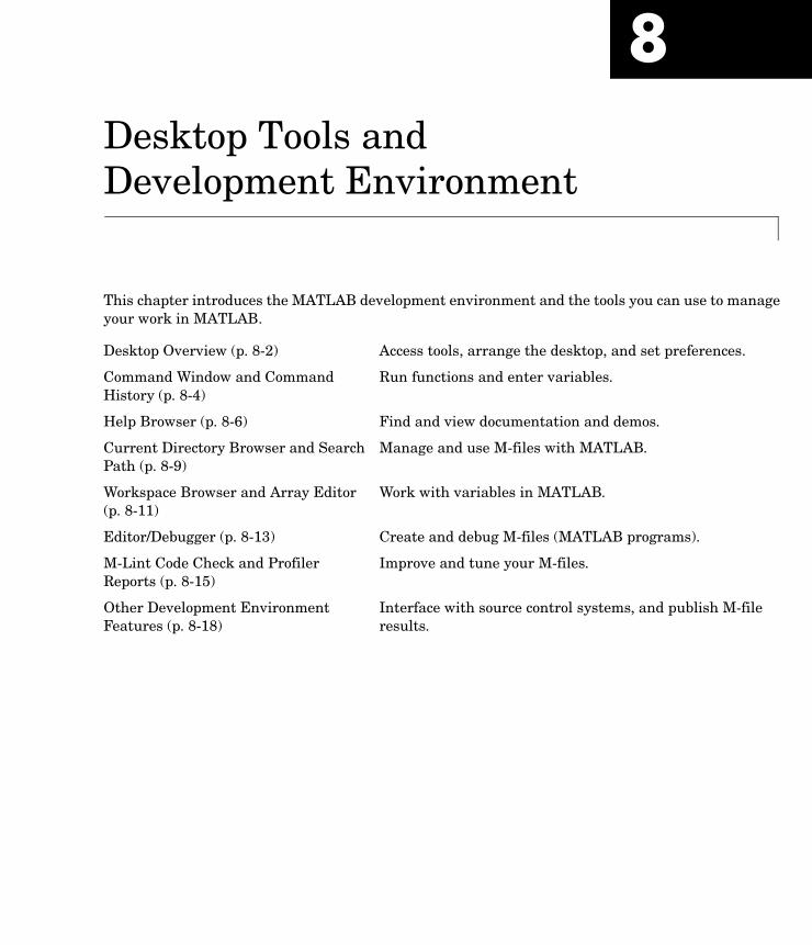
8
Desktop Tools and Development EnvironmentThis chapter introduces the MATLAB development environment and the tools you can use to manage your work in MATLAB.
Desktop Overview (p. 8-2) Access tools, arrange the desktop, and set preferences.
Command Window and Command History (p. 8-4)
Run functions and enter variables.
Help Browser (p. 8-6) Find and view documentation and demos.
Current Directory Browser and Search Path (p. 8-9)
Manage and use M-files with MATLAB.
Workspace Browser and Array Editor (p. 8-11)
Work with variables in MATLAB.
Editor/Debugger (p. 8-13) Create and debug M-files (MATLAB programs).
M-Lint Code Check and Profiler Reports (p. 8-15)
Improve and tune your M-files.
Other Development Environment Features (p. 8-18)
Interface with source control systems, and publish M-file results.
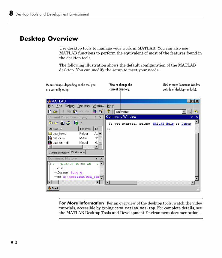
8 Desktop Tools and Development Environment
8-2
Desktop OverviewUse desktop tools to manage your work in MATLAB. You can also use MATLAB functions to perform the equivalent of most of the features found in the desktop tools.
The following illustration shows the default configuration of the MATLAB desktop. You can modify the setup to meet your needs.
For More Information For an overview of the desktop tools, watch the video tutorials, accessible by typing demo matlab desktop. For complete details, see the MATLAB Desktop Tools and Development Environment documentation.
View or change the current directory.
Click to move Command Window outside of desktop (undock).
Menus change, depending on the tool you are currently using.
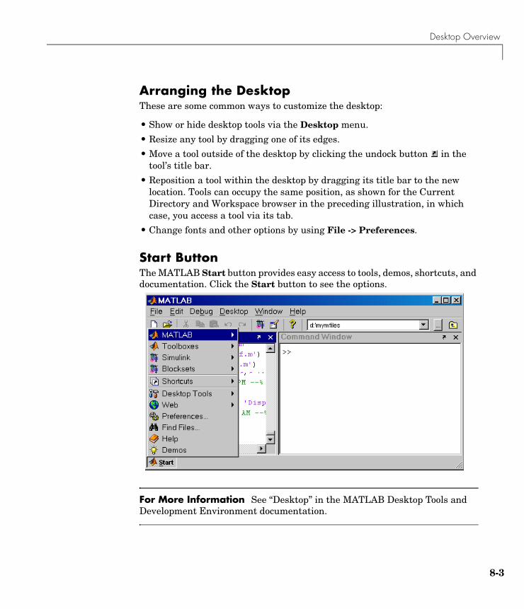
Desktop Overview
Arranging the DesktopThese are some common ways to customize the desktop:
• Show or hide desktop tools via the Desktop menu.
• Resize any tool by dragging one of its edges.
• Move a tool outside of the desktop by clicking the undock button in the tool’s title bar.
• Reposition a tool within the desktop by dragging its title bar to the new location. Tools can occupy the same position, as shown for the Current Directory and Workspace browser in the preceding illustration, in which case, you access a tool via its tab.
• Change fonts and other options by using File -> Preferences.
Start ButtonThe MATLAB Start button provides easy access to tools, demos, shortcuts, and documentation. Click the Start button to see the options.
For More Information See “Desktop” in the MATLAB Desktop Tools and Development Environment documentation.
8-3
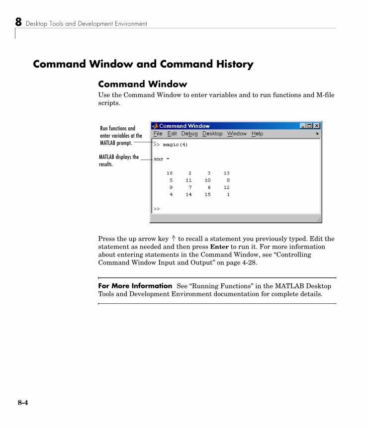
8 Desktop Tools and Development Environment
8-4
Command Window and Command History
Command WindowUse the Command Window to enter variables and to run functions and M-file scripts.
Press the up arrow key to recall a statement you previously typed. Edit the statement as needed and then press Enter to run it. For more information about entering statements in the Command Window, see “Controlling Command Window Input and Output” on page 4-28.
For More Information See “Running Functions” in the MATLAB Desktop Tools and Development Environment documentation for complete details.
Run functions and enter variables at the MATLAB prompt.
MATLAB displays the results.
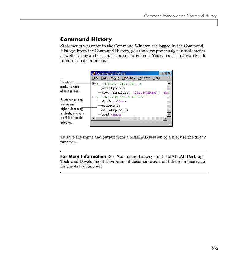
Command Window and Command History
Command HistoryStatements you enter in the Command Window are logged in the Command History. From the Command History, you can view previously run statements, as well as copy and execute selected statements. You can also create an M-file from selected statements.
To save the input and output from a MATLAB session to a file, use the diary function.
For More Information See “Command History” in the MATLAB Desktop Tools and Development Environment documentation, and the reference page for the diary function.
Timestamp marks the start of each session.
Select one or more entries and right-click to copy, evaluate, or create an M-file from the selection.
8-5
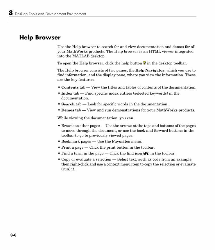
8 Desktop Tools and Development Environment
8-6
Help BrowserUse the Help browser to search for and view documentation and demos for all your MathWorks products. The Help browser is an HTML viewer integrated into the MATLAB desktop.
To open the Help browser, click the help button in the desktop toolbar.
The Help browser consists of two panes, the Help Navigator, which you use to find information, and the display pane, where you view the information. These are the key features:
• Contents tab — View the titles and tables of contents of the documentation.
• Index tab — Find specific index entries (selected keywords) in the documentation.
• Search tab — Look for specific words in the documentation.
• Demos tab — View and run demonstrations for your MathWorks products.
While viewing the documentation, you can
• Browse to other pages — Use the arrows at the tops and bottoms of the pages to move through the document, or use the back and forward buttons in the toolbar to go to previously viewed pages.
• Bookmark pages — Use the Favorites menu.
• Print a page — Click the print button in the toolbar.
• Find a term in the page — Click the find icon ( ) in the toolbar.
• Copy or evaluate a selection — Select text, such as code from an example, then right-click and use a context menu item to copy the selection or evaluate (run) it.
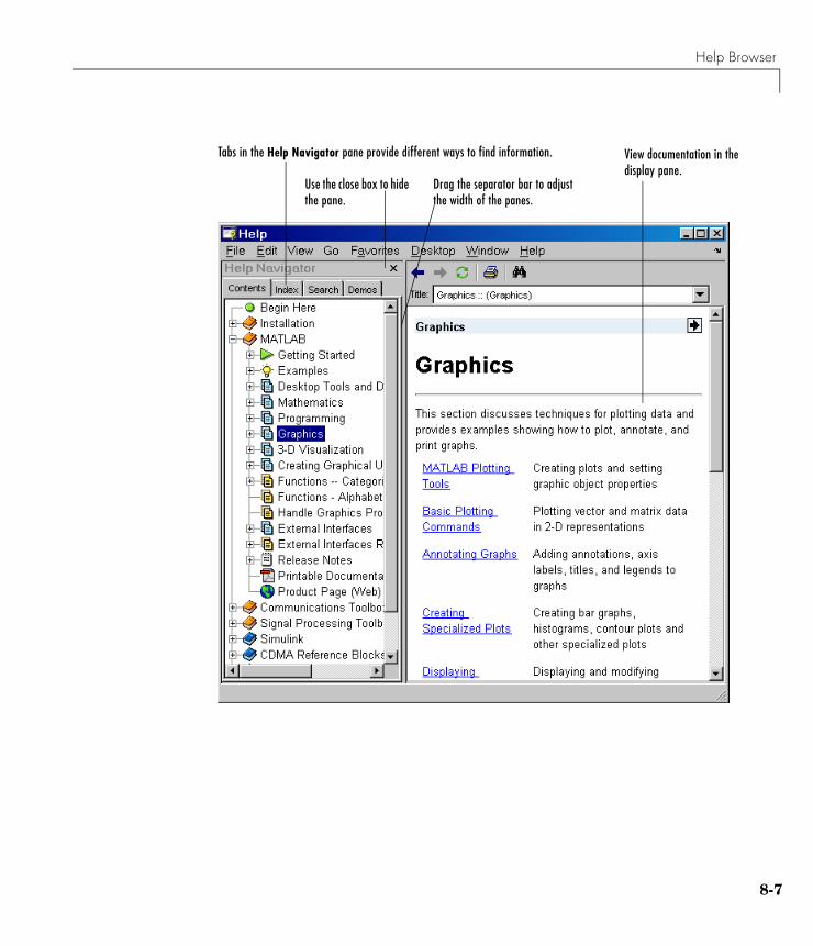
Help Browser
Tabs in the Help Navigator pane provide different ways to find information.
Drag the separator bar to adjust the width of the panes.
View documentation in the display pane.
Use the close box to hide the pane.
8-7
8 Desktop Tools and Development Environment
8-8
Other Forms of HelpIn addition to the Help browser, you can use help functions. To get help for a specific function, use the doc function. For example, doc format displays documentation for the format function in the Help browser.
To see a briefer form of the documentation for a function, type help followed by the function name. The resulting help text appears in the Command Window. It shows function names in all capital letters to distinguish them from the surrounding text. When you use the function names, type them in lowercase or they will not run. Some functions actually consist of both uppercase and lowercase letters, and the help text clearly indicates that. For those functions, match the case used in the help function.
Other means for getting help include contacting Technical Support (http://www.mathworks.com/support) and participating in the newsgroup for MATLAB users, comp.soft-sys.matlab.
For More Information See “Help for Using MATLAB” in the MATLAB Desktop Tools and Development Environment documentation, and the reference pages for the doc and help functions.
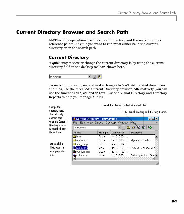
Current Directory Browser and Search Path
Current Directory Browser and Search PathMATLAB file operations use the current directory and the search path as reference points. Any file you want to run must either be in the current directory or on the search path.
Current DirectoryA quick way to view or change the current directory is by using the current directory field in the desktop toolbar, shown here.
To search for, view, open, and make changes to MATLAB related directories and files, use the MATLAB Current Directory browser. Alternatively, you can use the functions dir, cd, and delete. Use the Visual Directory and Directory Reports to help you manage M-files.
Change the directory here. This field only appears here when the Current Directory browser is undocked from the desktop.
Search for files and content within text files.
Double-click a file to open it in an appropriate tool.
For Visual Directory and Directory Reports
8-9
8 Desktop Tools and Development Environment
8-1
For More Information See “File Management Operations” in the MATLAB Desktop Tools and Development Environment documentation, and the reference pages for the dir, cd, and delete functions.
Search PathMATLAB uses a search path to find M-files and other MATLAB related files, which are organized in directories on your file system. Any file you want to run in MATLAB must reside in the current directory or in a directory that is on the search path. When you create M-files and related files for MATLAB, add the directories in which they are located to the MATLAB search path. By default, the files supplied with MATLAB and other MathWorks products are included in the search path.
To see which directories are on the search path or to change the search path, select File -> Set Path and use the resulting Set Path dialog box. Alternatively, you can use the path function to view the search path, addpath to add directories to the path, and rmpath to remove directories from the path.
For More Information See “Search Path” in the MATLAB Desktop Tools and Development Environment documentation, and the reference pages for the path, addpath, and rmpath functions.
0
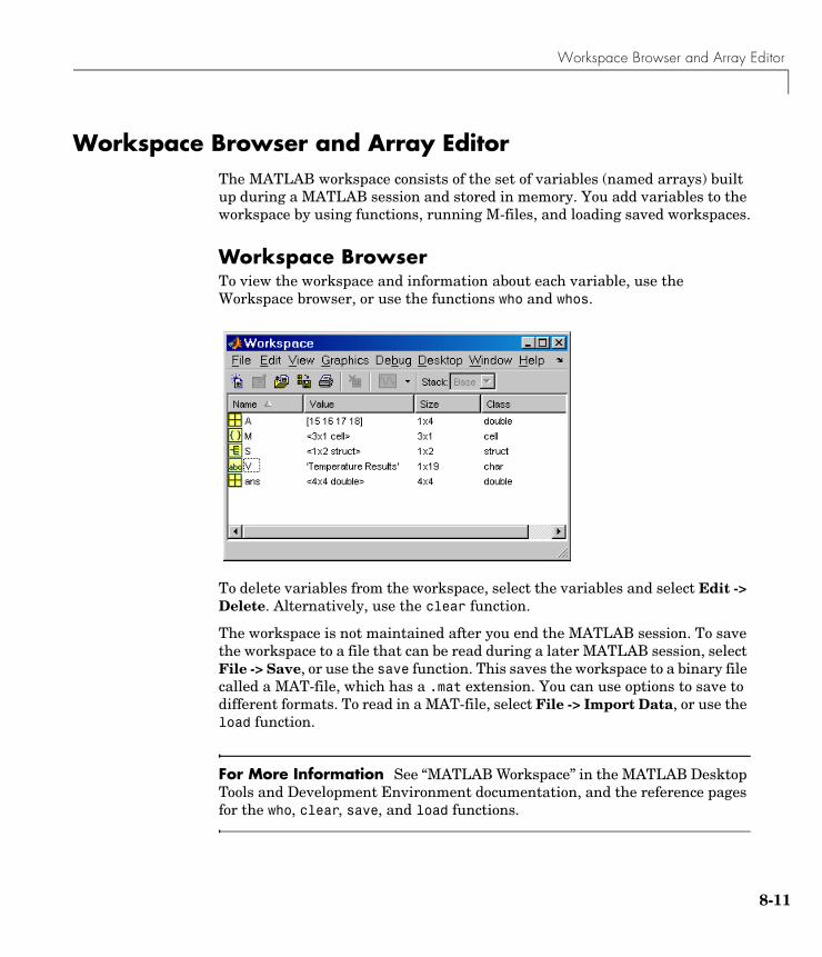
Workspace Browser and Array Editor
Workspace Browser and Array EditorThe MATLAB workspace consists of the set of variables (named arrays) built up during a MATLAB session and stored in memory. You add variables to the workspace by using functions, running M-files, and loading saved workspaces.
Workspace BrowserTo view the workspace and information about each variable, use the Workspace browser, or use the functions who and whos.
To delete variables from the workspace, select the variables and select Edit -> Delete. Alternatively, use the clear function.
The workspace is not maintained after you end the MATLAB session. To save the workspace to a file that can be read during a later MATLAB session, select File -> Save, or use the save function. This saves the workspace to a binary file called a MAT-file, which has a .mat extension. You can use options to save to different formats. To read in a MAT-file, select File -> Import Data, or use the load function.
For More Information See “MATLAB Workspace” in the MATLAB Desktop Tools and Development Environment documentation, and the reference pages for the who, clear, save, and load functions.
8-11
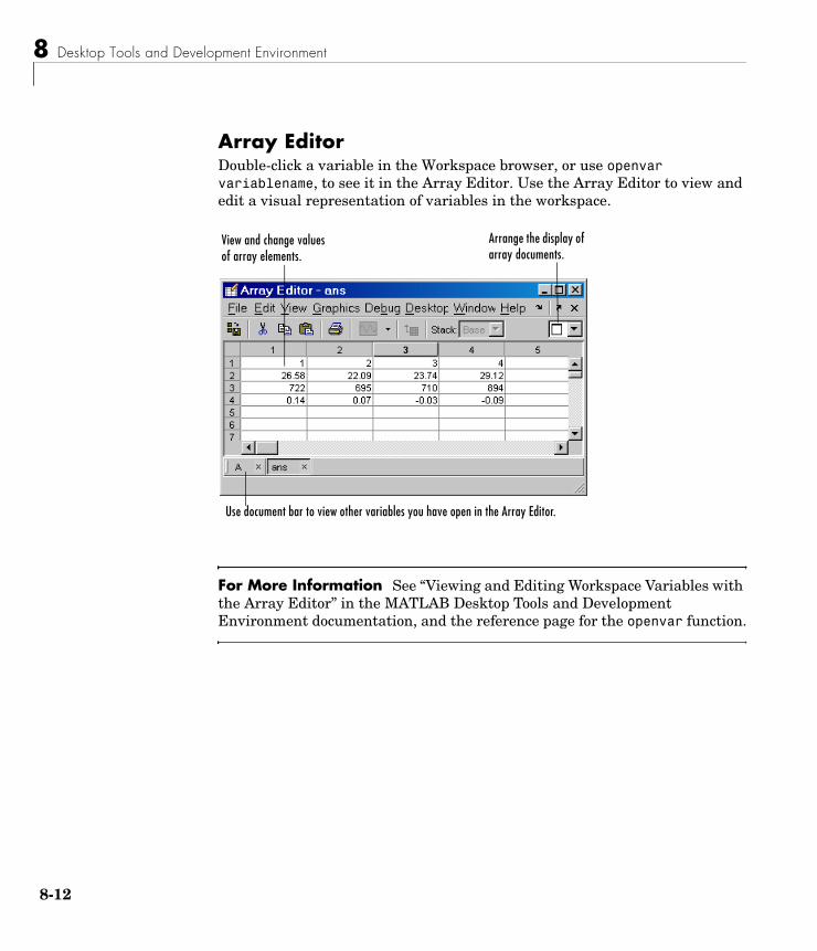
8 Desktop Tools and Development Environment
8-1
Array EditorDouble-click a variable in the Workspace browser, or use openvar variablename, to see it in the Array Editor. Use the Array Editor to view and edit a visual representation of variables in the workspace.
For More Information See “Viewing and Editing Workspace Variables with the Array Editor” in the MATLAB Desktop Tools and Development Environment documentation, and the reference page for the openvar function.
View and change values of array elements.
Use document bar to view other variables you have open in the Array Editor.
Arrange the display of array documents.
2
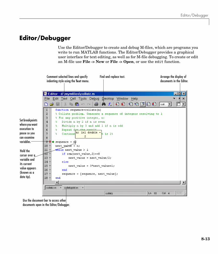
Editor/Debugger
Editor/DebuggerUse the Editor/Debugger to create and debug M-files, which are programs you write to run MATLAB functions. The Editor/Debugger provides a graphical user interface for text editing, as well as for M-file debugging. To create or edit an M-file use File -> New or File -> Open, or use the edit function.
Set breakpoints where you want execution to pause so you can examine variables.
Find and replace text.Comment selected lines and specify indenting style using the Text menu.
Hold the cursor over a variable and its current value appears (known as a data tip).
Use the document bar to access other documents open in the Editor/Debugger.
Arrange the display of documents in the Editor.
8-13
8 Desktop Tools and Development Environment
8-1
You can use any text editor to create M-files, such as Emacs. Use preferences (accessible from the desktop File menu) to specify that editor as the default. If you use another editor, you can still use the MATLAB Editor/Debugger for debugging, or you can use debugging functions, such as dbstop, which sets a breakpoint.
If you just need to view the contents of an M-file, you can display the contents in the Command Window using the type function.
For More Information See “Editing and Debugging M-Files” in the MATLAB Desktop Tools and Development Environment documentation, and the function reference pages for edit, type, and debug.
4
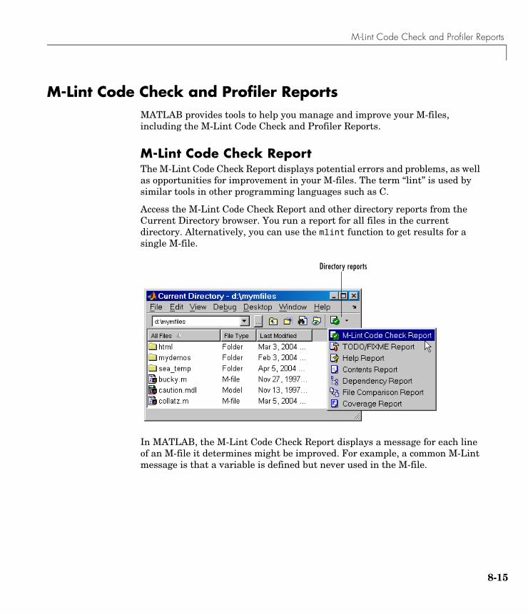
M-Lint Code Check and Profiler Reports
M-Lint Code Check and Profiler ReportsMATLAB provides tools to help you manage and improve your M-files, including the M-Lint Code Check and Profiler Reports.
M-Lint Code Check ReportThe M-Lint Code Check Report displays potential errors and problems, as well as opportunities for improvement in your M-files. The term “lint” is used by similar tools in other programming languages such as C.
Access the M-Lint Code Check Report and other directory reports from the Current Directory browser. You run a report for all files in the current directory. Alternatively, you can use the mlint function to get results for a single M-file.
In MATLAB, the M-Lint Code Check Report displays a message for each line of an M-file it determines might be improved. For example, a common M-Lint message is that a variable is defined but never used in the M-file.
Directory reports
8-15
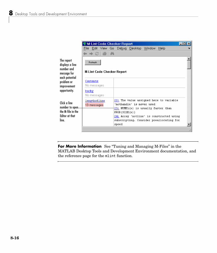
8 Desktop Tools and Development Environment
8-1
For More Information See “Tuning and Managing M-Files” in the MATLAB Desktop Tools and Development Environment documentation, and the reference page for the mlint function.
The report displays a line number and message for each potential problem or improvement opportunity.
Click a line number to open the M-file in the Editor at that line.
6
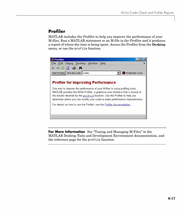
M-Lint Code Check and Profiler Reports
ProfilerMATLAB includes the Profiler to help you improve the performance of your M-files. Run a MATLAB statement or an M-file in the Profiler and it produces a report of where the time is being spent. Access the Profiler from the Desktop menu, or use the profile function.
For More Information See “Tuning and Managing M-Files” in the MATLAB Desktop Tools and Development Environment documentation, and the reference page for the profile function.
8-17
8 Desktop Tools and Development Environment
8-1
Other Development Environment FeaturesAdditional development environment features include
• Source Control — Access your source control system from within MATLAB.
• Publishing Results — Use the Editor’s cell features to publish M-files and results to popular output formats including HTML and Microsoft Word. You can also use MATLAB Notebook to access MATLAB functions from within Microsoft Word.
For More Information See “Source Control” and “Publishing Results” in the MATLAB Desktop Tools and Development Environment documentation.
8
9
Introducing the Symbolic Math ToolboxThis chapter introduces you to the Symbolic Math Toolbox, and describes how to create and use symbolic objects. It covers the following topics:
What Is the Symbolic Math Toolbox? (p. 9-2)
Overview of the toolbox
Symbolic Objects (p. 9-3) Describes symbolic objects and how they differ from standard MATLAB data types
Creating Symbolic Variables and Expressions (p. 9-5)
How to create symbolic objects
The subs Command (p. 9-8) How to substitute numbers for variables
Symbolic and Numeric Conversions (p. 9-10)
How to convert between symbolic objects and numeric values
Creating Symbolic Math Functions (p. 9-15)
How to create functions that operate on symbolic objects
9 Introducing the Symbolic Math Toolbox
9-2
What Is the Symbolic Math Toolbox?The Symbolic Math Toolbox incorporates symbolic computation into the numeric environment of MATLAB. The toolbox is a collection of more than 100 MATLAB functions that provide access to the Maple kernel using a syntax and style that is a natural extension of the MATLAB language. The Symbolic Math Toolbox supplements MATLAB numeric and graphical facilities with several other types of mathematical computation, which are summarized in following table.
The computational engine underlying the toolboxes is the kernel of Maple, a system developed primarily at the University of Waterloo, Canada and, more recently, at the Eidgenössiche Technische Hochschule, Zürich, Switzerland. Maple is marketed and supported by Waterloo Maple, Inc.
Facility Covers
Calculus Differentiation, integration, limits, summation, and Taylor series
Linear Algebra Inverses, determinants, eigenvalues, singular value decomposition, and canonical forms of symbolic matrices
Simplification Methods of simplifying algebraic expressions
Solution of Equations
Symbolic and numerical solutions to algebraic and differential equations
Variable-Precision Arithmetic
Numerical evaluation of mathematical expressions to any specified accuracy
Transforms Fourier, Laplace, z-transform, and corresponding inverse transforms
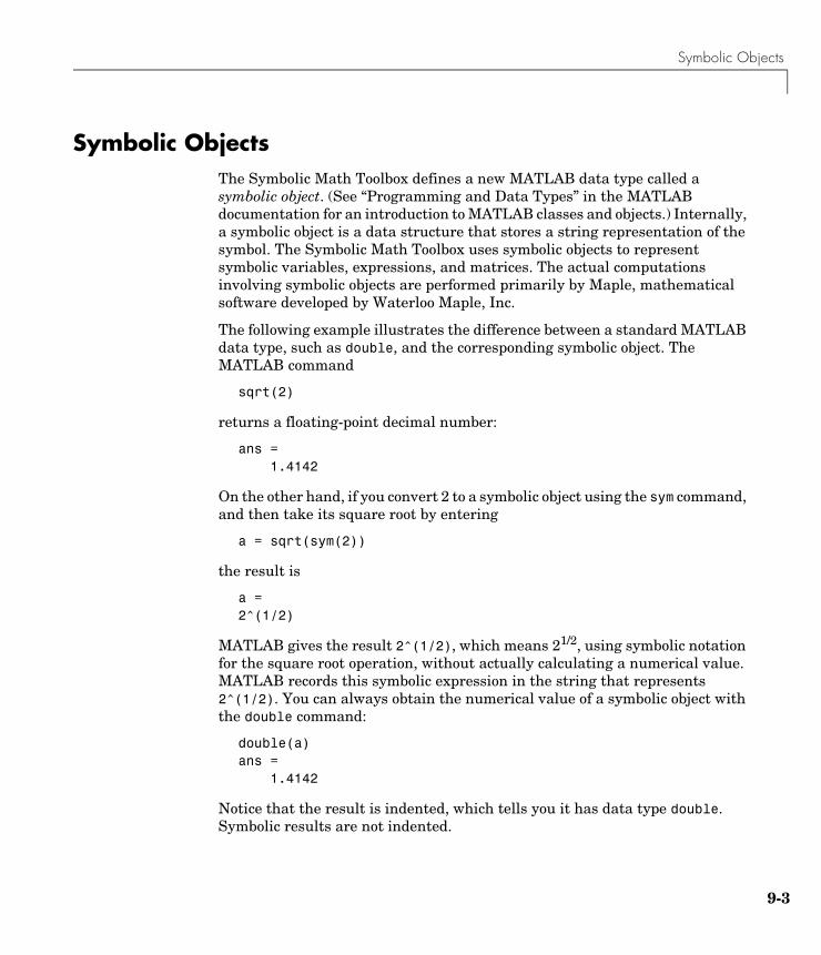
Symbolic Objects
Symbolic ObjectsThe Symbolic Math Toolbox defines a new MATLAB data type called a symbolic object. (See “Programming and Data Types” in the MATLAB documentation for an introduction to MATLAB classes and objects.) Internally, a symbolic object is a data structure that stores a string representation of the symbol. The Symbolic Math Toolbox uses symbolic objects to represent symbolic variables, expressions, and matrices. The actual computations involving symbolic objects are performed primarily by Maple, mathematical software developed by Waterloo Maple, Inc.
The following example illustrates the difference between a standard MATLAB data type, such as double, and the corresponding symbolic object. The MATLAB command
sqrt(2)
returns a floating-point decimal number:
ans =1.4142
On the other hand, if you convert 2 to a symbolic object using the sym command, and then take its square root by entering
a = sqrt(sym(2))
the result is
a =2^(1/2)
MATLAB gives the result 2^(1/2), which means 21/2, using symbolic notation for the square root operation, without actually calculating a numerical value. MATLAB records this symbolic expression in the string that represents 2^(1/2). You can always obtain the numerical value of a symbolic object with the double command:
double(a)ans =
1.4142
Notice that the result is indented, which tells you it has data type double. Symbolic results are not indented.
9-3
9 Introducing the Symbolic Math Toolbox
9-4
When you create a fraction involving symbolic objects, MATLAB records the numerator and denominator. For example:
sym(2)/sym(5)ans =2/5
MATLAB performs arithmetic on symbolic objects differently than it does on standard data types. If you add two fractions that are of data type double, MATLAB gives the answer as a decimal fraction. For example:
2/5 + 1/3ans =0.7333
If you add the same fractions as symbolic objects, MATLAB finds their common denominator and combines them by the usual procedure for adding rational numbers:
sym(2)/sym(5) + sym(1)/sym(3)ans =11/15
The Symbolic Math Toolbox enables you to perform a variety of symbolic calculations that arise in mathematics and science. These are described in detail in Chapter 10, “Using the Symbolic Math Toolbox.”
Creating Symbolic Variables and Expressions
Creating Symbolic Variables and ExpressionsThe sym command lets you construct symbolic variables and expressions. For example, the commands
x = sym('x')a = sym('alpha')
create a symbolic variable x that prints as x and a symbolic variable a that prints as alpha.
Suppose you want to use a symbolic variable to represent the golden ratio
The command
rho = sym('(1 + sqrt(5))/2')
achieves this goal. Now you can perform various mathematical operations on rho. For example,
f = rho^2 - rho - 1
returns
f = (1/2+1/2*5^(1/2))^2-3/2-1/2*5^(1/2)
You can simplify this answer by entering
simplify(f)
which returns
ans =0
Now suppose you want to study the quadratic function . One approach is to enter the command
f = sym('a*x^2 + b*x + c')
ρ 1 5+2
-----------------=
f ax2 bx c+ +=
9-5
9 Introducing the Symbolic Math Toolbox
9-6
which assigns the symbolic expression to the variable f. However, in this case, the Symbolic Math Toolbox does not create variables corresponding to the terms of the expression, , , , and . To perform symbolic math operations (e.g., integration, differentiation, substitution, etc.) on f, you need to create the variables explicitly. A better alternative is to enter the commands
a = sym('a')b = sym('b')c = sym('c')x = sym('x')
or simply
syms a b c x
Then enter
f = sym('a*x^2 + b*x + c')
In general, you can use sym or syms to create symbolic variables. We recommend you use syms because it requires less typing.
Note To create a symbolic expression that is a constant, you must use the sym command. For example, to create the expression whose value is 5, enter f = sym('5'). Note that the command f = 5 does not define f as a symbolic expression.
If you set a variable equal to a symbolic expression, and then apply the syms command to the variable, MATLAB removes the previously defined expression from the variable. For example,
syms a bf = a + b
returns
f =a+b
ax2 bx c+ +
a b c x
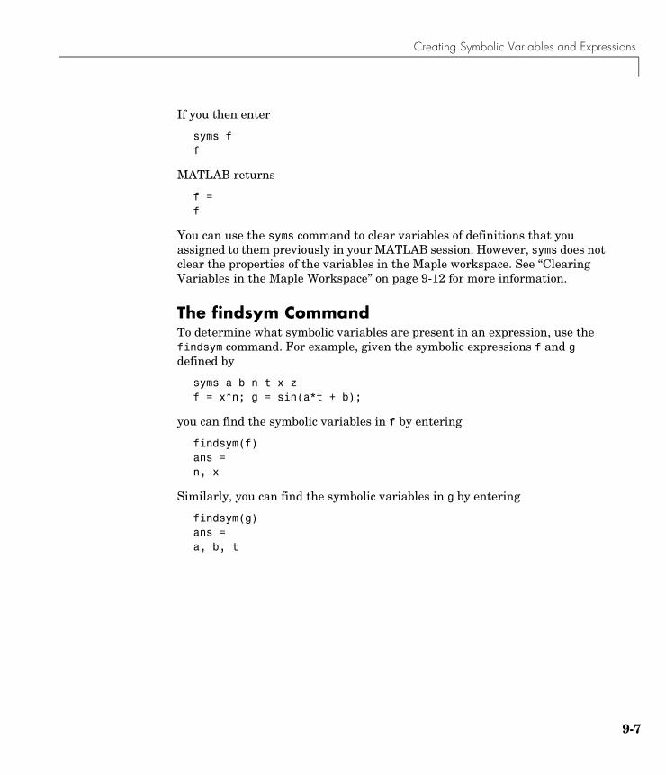
Creating Symbolic Variables and Expressions
If you then enter
syms ff
MATLAB returns
f =f
You can use the syms command to clear variables of definitions that you assigned to them previously in your MATLAB session. However, syms does not clear the properties of the variables in the Maple workspace. See “Clearing Variables in the Maple Workspace” on page 9-12 for more information.
The findsym CommandTo determine what symbolic variables are present in an expression, use the findsym command. For example, given the symbolic expressions f and g defined by
syms a b n t x zf = x^n; g = sin(a*t + b);
you can find the symbolic variables in f by entering
findsym(f)ans = n, x
Similarly, you can find the symbolic variables in g by entering
findsym(g)ans = a, b, t
9-7
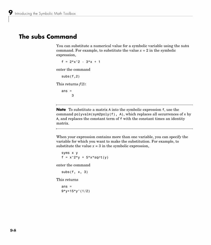
9 Introducing the Symbolic Math Toolbox
9-8
The subs CommandYou can substitute a numerical value for a symbolic variable using the subs command. For example, to substitute the value x = 2 in the symbolic expression,
f = 2*x^2 - 3*x + 1
enter the command
subs(f,2)
This returns f(2):
ans =3
Note To substitute a matrix A into the symbolic expression f, use the command polyvalm(sym2poly(f), A), which replaces all occurrences of x by A, and replaces the constant term of f with the constant times an identity matrix.
When your expression contains more than one variable, you can specify the variable for which you want to make the substitution. For example, to substitute the value x = 3 in the symbolic expression,
syms x yf = x^2*y + 5*x*sqrt(y)
enter the command
subs(f, x, 3)
This returns
ans = 9*y+15*y^(1/2)
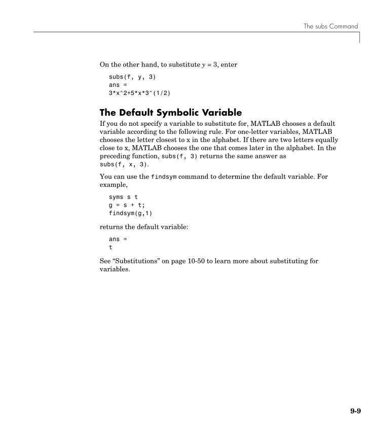
The subs Command
On the other hand, to substitute y = 3, enter
subs(f, y, 3)ans = 3*x^2+5*x*3^(1/2)
The Default Symbolic VariableIf you do not specify a variable to substitute for, MATLAB chooses a default variable according to the following rule. For one-letter variables, MATLAB chooses the letter closest to x in the alphabet. If there are two letters equally close to x, MATLAB chooses the one that comes later in the alphabet. In the preceding function, subs(f, 3) returns the same answer as subs(f, x, 3).
You can use the findsym command to determine the default variable. For example,
syms s tg = s + t;findsym(g,1)
returns the default variable:
ans = t
See “Substitutions” on page 10-50 to learn more about substituting for variables.
9-9
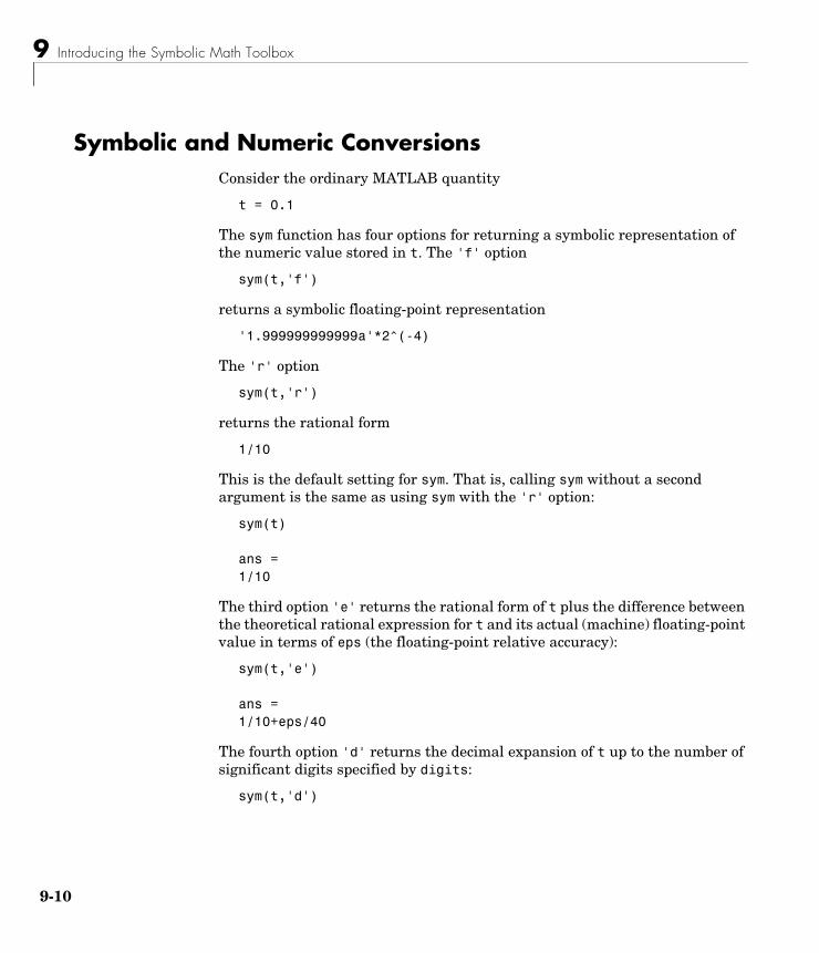
9 Introducing the Symbolic Math Toolbox
9-1
Symbolic and Numeric ConversionsConsider the ordinary MATLAB quantity
t = 0.1
The sym function has four options for returning a symbolic representation of the numeric value stored in t. The 'f' option
sym(t,'f')
returns a symbolic floating-point representation
'1.999999999999a'*2^(-4)
The 'r' option
sym(t,'r')
returns the rational form
1/10
This is the default setting for sym. That is, calling sym without a second argument is the same as using sym with the 'r' option:
sym(t) ans =1/10
The third option 'e' returns the rational form of t plus the difference between the theoretical rational expression for t and its actual (machine) floating-point value in terms of eps (the floating-point relative accuracy):
sym(t,'e') ans =1/10+eps/40
The fourth option 'd' returns the decimal expansion of t up to the number of significant digits specified by digits:
sym(t,'d')
0
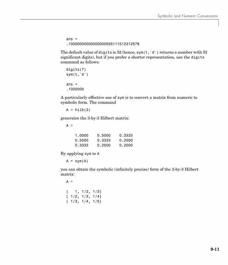
Symbolic and Numeric Conversions
ans =.10000000000000000555111512312578
The default value of digits is 32 (hence, sym(t,'d') returns a number with 32 significant digits), but if you prefer a shorter representation, use the digits command as follows:
digits(7)sym(t,'d') ans =.1000000
A particularly effective use of sym is to convert a matrix from numeric to symbolic form. The command
A = hilb(3)
generates the 3-by-3 Hilbert matrix:
A = 1.0000 0.5000 0.3333 0.5000 0.3333 0.2500 0.3333 0.2500 0.2000
By applying sym to A
A = sym(A)
you can obtain the symbolic (infinitely precise) form of the 3-by-3 Hilbert matrix:
A = [ 1, 1/2, 1/3][ 1/2, 1/3, 1/4][ 1/3, 1/4, 1/5]
9-11
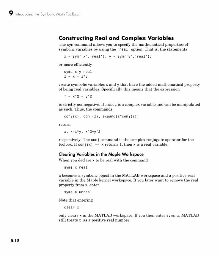
9 Introducing the Symbolic Math Toolbox
9-1
Constructing Real and Complex VariablesThe sym command allows you to specify the mathematical properties of symbolic variables by using the 'real' option. That is, the statements
x = sym('x','real'); y = sym('y','real');
or more efficiently
syms x y realz = x + i*y
create symbolic variables x and y that have the added mathematical property of being real variables. Specifically this means that the expression
f = x^2 + y^2
is strictly nonnegative. Hence, z is a complex variable and can be manipulated as such. Thus, the commands
conj(x), conj(z), expand(z*conj(z))
return
x, x-i*y, x^2+y^2
respectively. The conj command is the complex conjugate operator for the toolbox. If conj(x) == x returns 1, then x is a real variable.
Clearing Variables in the Maple WorkspaceWhen you declare x to be real with the command
syms x real
a becomes a symbolic object in the MATLAB workspace and a positive real variable in the Maple kernel workspace. If you later want to remove the real property from x, enter
syms a unreal
Note that entering
clear x
only clears x in the MATLAB workspace. If you then enter syms x, MATLAB still treats x as a positive real number.
2
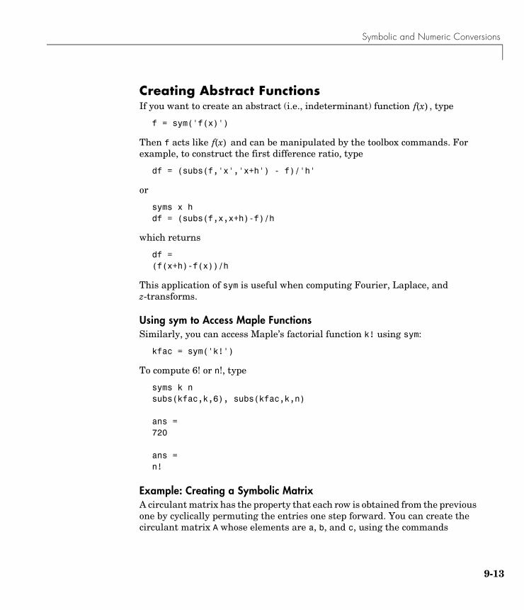
Symbolic and Numeric Conversions
Creating Abstract FunctionsIf you want to create an abstract (i.e., indeterminant) function , type
f = sym('f(x)')
Then f acts like and can be manipulated by the toolbox commands. For example, to construct the first difference ratio, type
df = (subs(f,'x','x+h') - f)/'h'
or
syms x hdf = (subs(f,x,x+h)-f)/h
which returns
df =(f(x+h)-f(x))/h
This application of sym is useful when computing Fourier, Laplace, and z-transforms.
Using sym to Access Maple FunctionsSimilarly, you can access Maple’s factorial function k! using sym:
kfac = sym('k!')
To compute 6! or n!, type
syms k nsubs(kfac,k,6), subs(kfac,k,n) ans =720
ans =n!
Example: Creating a Symbolic MatrixA circulant matrix has the property that each row is obtained from the previous one by cyclically permuting the entries one step forward. You can create the circulant matrix A whose elements are a, b, and c, using the commands
f x( )
f x( )
9-13
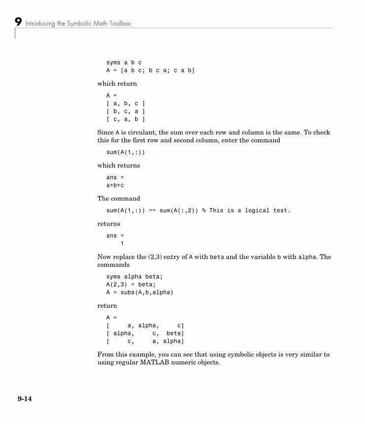
9 Introducing the Symbolic Math Toolbox
9-1
syms a b cA = [a b c; b c a; c a b]
which return
A = [ a, b, c ][ b, c, a ][ c, a, b ]
Since A is circulant, the sum over each row and column is the same. To check this for the first row and second column, enter the command
sum(A(1,:))
which returns
ans =a+b+c
The command
sum(A(1,:)) == sum(A(:,2)) % This is a logical test.
returns
ans =1
Now replace the (2,3) entry of A with beta and the variable b with alpha. The commands
syms alpha beta;A(2,3) = beta;A = subs(A,b,alpha)
return
A = [ a, alpha, c][ alpha, c, beta][ c, a, alpha]
From this example, you can see that using symbolic objects is very similar to using regular MATLAB numeric objects.
4
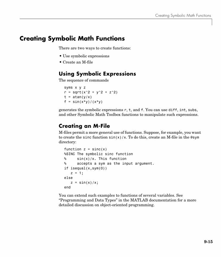
Creating Symbolic Math Functions
Creating Symbolic Math FunctionsThere are two ways to create functions:
• Use symbolic expressions
• Create an M-file
Using Symbolic ExpressionsThe sequence of commands
syms x y zr = sqrt(x^2 + y^2 + z^2)t = atan(y/x)f = sin(x*y)/(x*y)
generates the symbolic expressions r, t, and f. You can use diff, int, subs, and other Symbolic Math Toolbox functions to manipulate such expressions.
Creating an M-FileM-files permit a more general use of functions. Suppose, for example, you want to create the sinc function sin(x)/x. To do this, create an M-file in the @sym directory:
function z = sinc(x)%SINC The symbolic sinc function% sin(x)/x. This function% accepts a sym as the input argument.if isequal(x,sym(0)) z = 1;else z = sin(x)/x;end
You can extend such examples to functions of several variables. See “Programming and Data Types” in the MATLAB documentation for a more detailed discussion on object-oriented programming.
9-15

9 Introducing the Symbolic Math Toolbox
9-1
6
10
Using the Symbolic Math ToolboxThis chapter explains how to use the Symbolic Math Toolbox to perform many common mathematical operations. It covers the following topics:
Calculus (p. 10-2) Differentiation, integration, limits, summation, and Taylor series
Simplifications and Substitutions (p. 10-41)
Methods of simplifying algebraic expressions
Variable-Precision Arithmetic (p. 10-57)
Numerical evaluation of mathematical expressions to any specified accuracy
Linear Algebra (p. 10-62) Inverses, determinants, eigenvalues, singular value decomposition, and canonical forms of symbolic matrices
Solving Equations (p. 10-86) Symbolic and numerical solutions to algebraic and differential equations
10 Using the Symbolic Math Toolbox
10-
CalculusThe Symbolic Math Toolbox provides functions to do the basic operations of calculus. The following sections describe these functions:
• “Differentiation” on page 10-2
• “Limits” on page 10-8
• “Integration” on page 10-11
• “Symbolic Summation” on page 10-18
• “Taylor Series” on page 10-18
• “Calculus Example” on page 10-20
• “Extended Calculus Example” on page 10-28
DifferentiationTo illustrate how to take derivatives using the Symbolic Math Toolbox, first create a symbolic expression:
syms x f = sin(5*x)
The command
diff(f)
differentiates f with respect to x:
ans =5*cos(5*x)
As another example, let
g = exp(x)*cos(x)
where exp(x) denotes ex, and differentiate g:
diff(g)ans =exp(x)*cos(x)-exp(x)*sin(x)
2
Calculus
To take the second derivative of g, enter
diff(g,2)ans =-2*exp(x)*sin(x)
You can get the same result by taking the derivative twice:
diff(diff(g))ans =-2*exp(x)*sin(x)
In this example, MATLAB automatically simplifies the answer. However, in some cases, MATLAB might not simply an answer, in which case you can use the simplify command. For an example of this, see “More Examples” on page 10-5.
Note that to take the derivative of a constant, you must first define the constant as a symbolic expression. For example, entering
c = sym('5');diff(c)
returns
ans =0
If you just enter
diff(5)
MATLAB returns
ans = []
because 5 is not a symbolic expression.
Derivatives of Expressions with Several VariablesTo differentiate an expression that contains more than one symbolic variable, you must specify the variable that you want to differentiate with respect to. The diff command then calculates the partial derivative of the expression with respect to that variable. For example, given the symbolic expression
10-3
10 Using the Symbolic Math Toolbox
10-
syms s tf = sin(s*t)
the command
diff(f,t)
calculates the partial derivative . The result is
ans = cos(s*t)*s
To differentiate f with respect to the variable s, enter
diff(f,s)
which returns:
ans =cos(s*t)*t
If you do not specify a variable to differentiate with respect to, MATLAB chooses a default variable by the same rule described in “The subs Command” on page 9-8. For one-letter variables, the default variable is the letter closest to x in the alphabet. In the preceding example, diff(f) takes the derivative of f with respect to t because t is closer to x in the alphabet than s is. To determine the default variable that MATLAB differentiates with respect to, use the findsym command:
findsym(f,1)ans = t
To calculate the second derivative of f with respect to t, enter
diff(f,t,2)
which returns
ans =-sin(s*t)*s^2
Note that diff(f,2) returns the same answer because t is the default variable.
f∂ t∂⁄
4
Calculus
More ExamplesTo further illustrate the diff command, define a, b, x, n, t, and theta in the MATLAB workspace by entering
syms a b x n t theta
The table below illustrates the results of entering diff(f).
In the first example, MATLAB does not automatically simplify the answer. To simplify the answer, enter
simplify(diff(x^n))ans =x^(n-1)*n
To differentiate the Bessel function of the first kind, besselj(nu,z), with respect to z, type
syms nu zb = besselj(nu,z);db = diff(b)
which returns
db =-besselj(nu+1,z)+nu/z*besselj(nu,z)
The diff function can also take a symbolic matrix as its input. In this case, the differentiation is done element-by-element. Consider the example
syms a xA = [cos(a*x),sin(a*x);-sin(a*x),cos(a*x)]
f diff(f)
x^n x^n*n/x
sin(a*t+b) cos(a*t+b)*a
exp(i*theta) i*exp(i*theta)
10-5
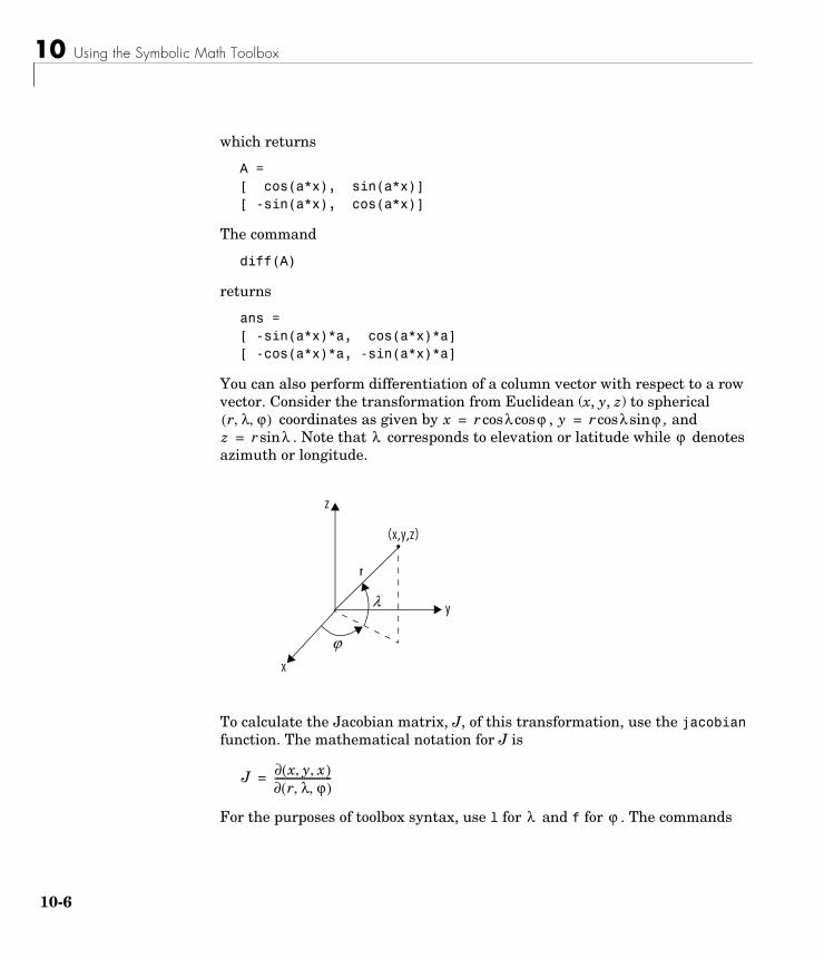
10 Using the Symbolic Math Toolbox
10-
which returns
A =[ cos(a*x), sin(a*x)][ -sin(a*x), cos(a*x)]
The command
diff(A)
returns
ans =[ -sin(a*x)*a, cos(a*x)*a][ -cos(a*x)*a, -sin(a*x)*a]
You can also perform differentiation of a column vector with respect to a row vector. Consider the transformation from Euclidean (x, y, z) to spherical
coordinates as given by , , and . Note that corresponds to elevation or latitude while denotes
azimuth or longitude.
To calculate the Jacobian matrix, J, of this transformation, use the jacobian function. The mathematical notation for J is
For the purposes of toolbox syntax, use l for and f for . The commands
r λ ϕ, ,( ) x r λ ϕcoscos= y r λ ϕsincos=z r λsin= λ ϕ
z
y
x
(x,y,z)
ϕ
λ
r
J x y x, ,( )∂r λ ϕ, ,( )∂
-----------------------=
λ ϕ
6
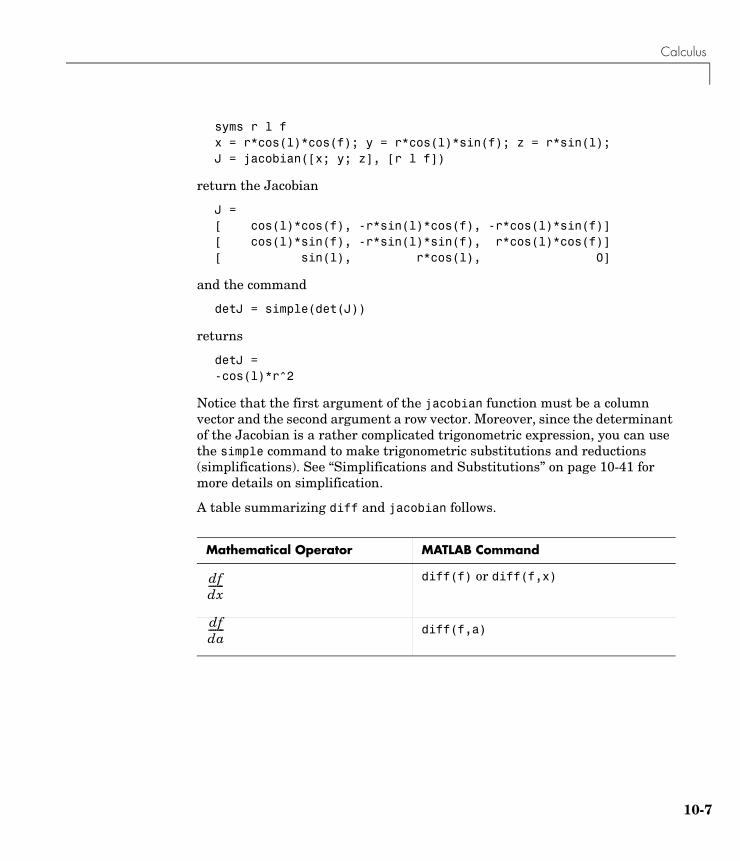
Calculus
syms r l fx = r*cos(l)*cos(f); y = r*cos(l)*sin(f); z = r*sin(l);J = jacobian([x; y; z], [r l f])
return the Jacobian
J =[ cos(l)*cos(f), -r*sin(l)*cos(f), -r*cos(l)*sin(f)][ cos(l)*sin(f), -r*sin(l)*sin(f), r*cos(l)*cos(f)][ sin(l), r*cos(l), 0]
and the command
detJ = simple(det(J))
returns
detJ = -cos(l)*r^2
Notice that the first argument of the jacobian function must be a column vector and the second argument a row vector. Moreover, since the determinant of the Jacobian is a rather complicated trigonometric expression, you can use the simple command to make trigonometric substitutions and reductions (simplifications). See “Simplifications and Substitutions” on page 10-41 for more details on simplification.
A table summarizing diff and jacobian follows.
Mathematical Operator MATLAB Command
diff(f) or diff(f,x)
diff(f,a)
dfdx-------
dfda-------
10-7
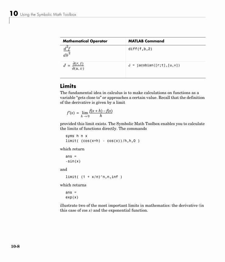
10 Using the Symbolic Math Toolbox
10-
LimitsThe fundamental idea in calculus is to make calculations on functions as a variable “gets close to” or approaches a certain value. Recall that the definition of the derivative is given by a limit
provided this limit exists. The Symbolic Math Toolbox enables you to calculate the limits of functions directly. The commands
syms h n xlimit( (cos(x+h) - cos(x))/h,h,0 )
which return
ans =-sin(x)
and
limit( (1 + x/n)^n,n,inf )
which returns
ans =exp(x)
illustrate two of the most important limits in mathematics: the derivative (in this case of cos x) and the exponential function.
diff(f,b,2)
J = jacobian([r;t],[u,v])
Mathematical Operator MATLAB Command
d2f
db2----------
J r t,( )∂u v,( )∂
-----------------=
f ′ x( ) f x h+( ) f x( )–h
----------------------------------h 0→lim=
8
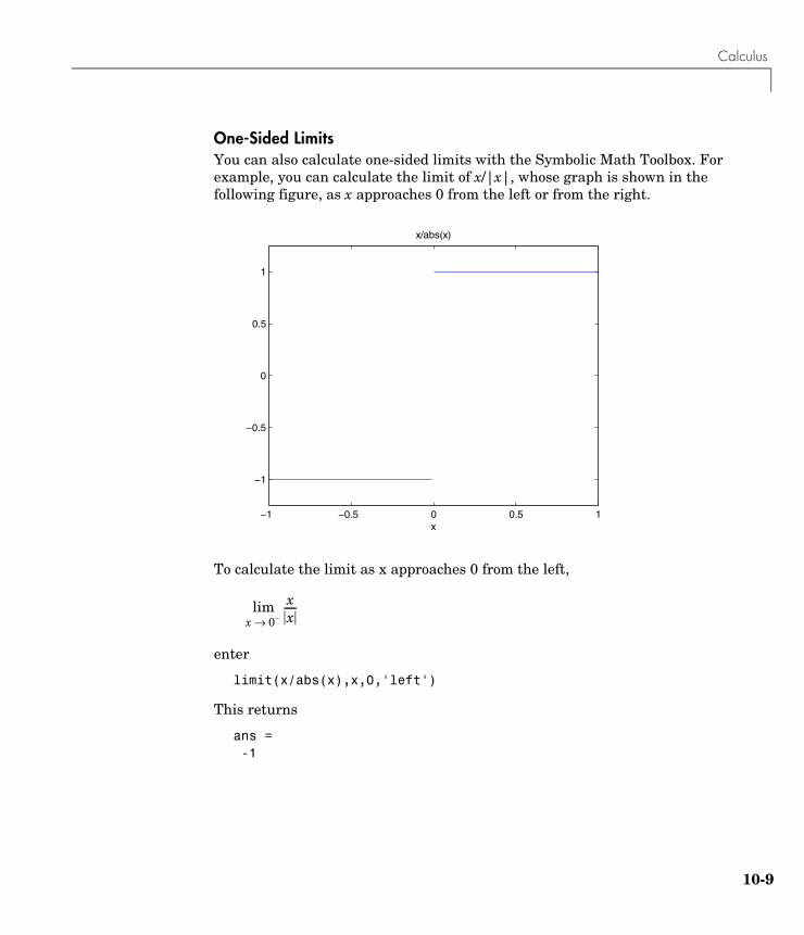
Calculus
One-Sided LimitsYou can also calculate one-sided limits with the Symbolic Math Toolbox. For example, you can calculate the limit of x/|x|, whose graph is shown in the following figure, as x approaches 0 from the left or from the right.
To calculate the limit as x approaches 0 from the left,
enter
limit(x/abs(x),x,0,'left')
This returns
ans = -1
−1 −0.5 0 0.5 1
−1
−0.5
0
0.5
1
x
x/abs(x)
xx-----
x 0–→lim
10-9
10 Using the Symbolic Math Toolbox
10-
To calculate the limit as x approaches 0 from the right,
enter
limit(x/abs(x),x,0,'right')
This returns
ans =1
Since the limit from the left does not equal the limit from the right, the two- sided limit does not exist. In the case of undefined limits, MATLAB returns NaN (not a number). For example,
limit(x/abs(x),x,0)
returns
ans =NaN
Observe that the default case, limit(f) is the same as limit(f,x,0). Explore the options for the limit command in this table, where f is a function of the symbolic object x.
Mathematical Operation MATLAB Command
limit(f)
limit(f,x,a) orlimit(f,a)
limit(f,x,a,'left')
limit(f,x,a,'right')
xx-----
x 0 +→lim 1=
f x( )x 0→lim
f x( )x a→lim
f x( )x a-→lim
f x( )x a+→lim
10
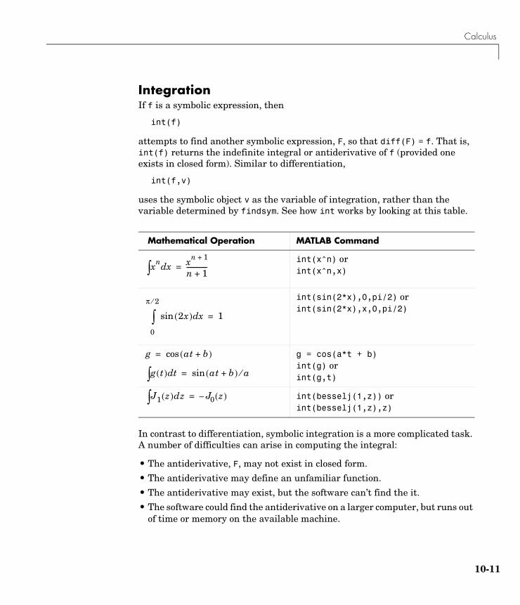
Calculus
IntegrationIf f is a symbolic expression, then
int(f)
attempts to find another symbolic expression, F, so that diff(F) = f. That is, int(f) returns the indefinite integral or antiderivative of f (provided one exists in closed form). Similar to differentiation,
int(f,v)
uses the symbolic object v as the variable of integration, rather than the variable determined by findsym. See how int works by looking at this table.
In contrast to differentiation, symbolic integration is a more complicated task. A number of difficulties can arise in computing the integral:
• The antiderivative, F, may not exist in closed form.
• The antiderivative may define an unfamiliar function.
• The antiderivative may exist, but the software can’t find the it.
• The software could find the antiderivative on a larger computer, but runs out of time or memory on the available machine.
Mathematical Operation MATLAB Command
int(x^n) orint(x^n,x)
int(sin(2*x),0,pi/2) or int(sin(2*x),x,0,pi/2)
g = cos(a*t + b)int(g) orint(g,t)
int(besselj(1,z)) orint(besselj(1,z),z)
xn xd∫ xn 1+
n 1+-------------=
2x( )sin xd
0
π 2⁄
∫ 1=
g at b+( )cos=
g t( ) td∫ at b+( )sin a⁄=
J1 z( )∫ dz J– 0 z( )=
10-11
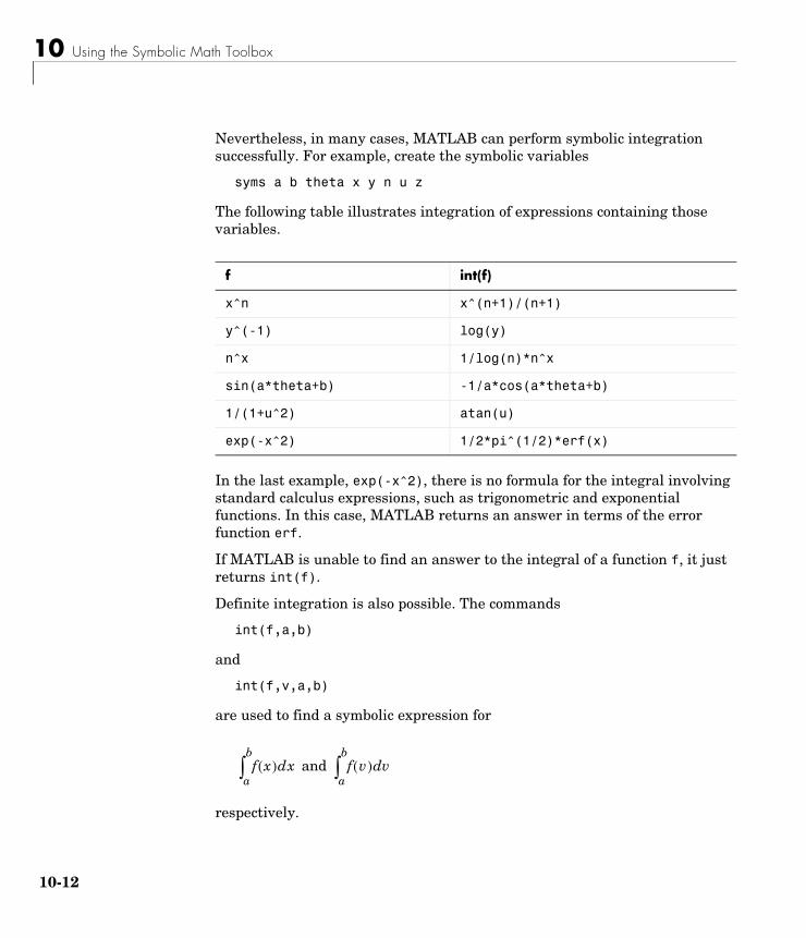
10 Using the Symbolic Math Toolbox
10-
Nevertheless, in many cases, MATLAB can perform symbolic integration successfully. For example, create the symbolic variables
syms a b theta x y n u z
The following table illustrates integration of expressions containing those variables.
In the last example, exp(-x^2), there is no formula for the integral involving standard calculus expressions, such as trigonometric and exponential functions. In this case, MATLAB returns an answer in terms of the error function erf.
If MATLAB is unable to find an answer to the integral of a function f, it just returns int(f).
Definite integration is also possible. The commands
int(f,a,b)
and
int(f,v,a,b)
are used to find a symbolic expression for
respectively.
f int(f)
x^n x^(n+1)/(n+1)
y^(-1) log(y)
n^x 1/log(n)*n^x
sin(a*theta+b) -1/a*cos(a*theta+b)
1/(1+u^2) atan(u)
exp(-x^2) 1/2*pi^(1/2)*erf(x)
and f x( )a
b
∫ dx f v( ) vda
b
∫
12
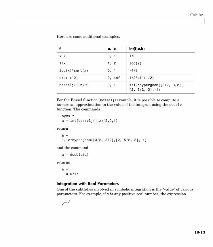
Calculus
Here are some additional examples.
For the Bessel function (besselj) example, it is possible to compute a numerical approximation to the value of the integral, using the double function. The commands
syms za = int(besselj(1,z)^2,0,1)
return
a =1/12*hypergeom([3/2, 3/2],[2, 5/2, 3],-1)
and the command
a = double(a)
returns
a = 0.0717
Integration with Real ParametersOne of the subtleties involved in symbolic integration is the “value” of various parameters. For example, if a is any positive real number, the expression
f a, b int(f,a,b)
x^7 0, 1 1/8
1/x 1, 2 log(2)
log(x)*sqrt(x) 0, 1 -4/9
exp(-x^2) 0, inf 1/2*pi^(1/2)
besselj(1,z)^2 0, 1 1/12*hypergeom([3/2, 3/2],[2, 5/2, 3],-1)
e a– x2
10-13
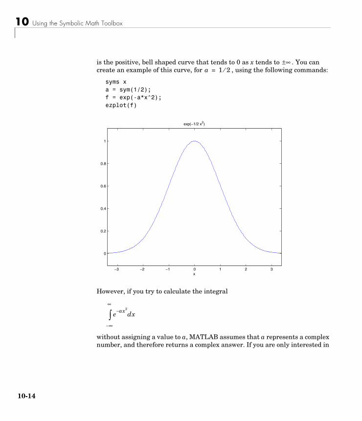
10 Using the Symbolic Math Toolbox
10-
is the positive, bell shaped curve that tends to 0 as x tends to . You can create an example of this curve, for , using the following commands:
syms xa = sym(1/2);f = exp(-a*x^2);ezplot(f)
However, if you try to calculate the integral
without assigning a value to a, MATLAB assumes that a represents a complex number, and therefore returns a complex answer. If you are only interested in
∞±a 1 2⁄=
−3 −2 −1 0 1 2 3
0
0.2
0.4
0.6
0.8
1
x
exp(−1/2 x2)
e ax2–
∞–
∞
∫ dx
14
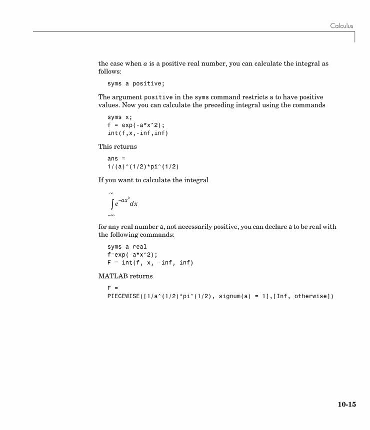
Calculus
the case when a is a positive real number, you can calculate the integral as follows:
syms a positive;
The argument positive in the syms command restricts a to have positive values. Now you can calculate the preceding integral using the commands
syms x;f = exp(-a*x^2);int(f,x,-inf,inf)
This returns
ans =1/(a)^(1/2)*pi^(1/2)
If you want to calculate the integral
for any real number a, not necessarily positive, you can declare a to be real with the following commands:
syms a realf=exp(-a*x^2);F = int(f, x, -inf, inf)
MATLAB returns
F =PIECEWISE([1/a^(1/2)*pi^(1/2), signum(a) = 1],[Inf, otherwise])
e ax– 2
∞–
∞
∫ dx
10-15
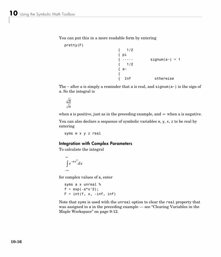
10 Using the Symbolic Math Toolbox
10-
You can put this in a more readable form by entering
pretty(F) { 1/2 { pi { ----- signum(a~) = 1 { 1/2 { a~ { { Inf otherwise
The ~ after a is simply a reminder that a is real, and signum(a~) is the sign of a. So the integral is
when a is positive, just as in the preceding example, and when a is negative.
You can also declare a sequence of symbolic variables w, y, x, z to be real by entering
syms w x y z real
Integration with Complex ParametersTo calculate the integral
for complex values of a, enter
syms a x unreal % f = exp(-a*x^2);F = int(f, x, -inf, inf)
Note that syms is used with the unreal option to clear the real property that was assigned to a in the preceding example — see “Clearing Variables in the Maple Workspace” on page 9-12.
πa
-------
∞
e ax– 2
∞–
∞
∫ dx
16
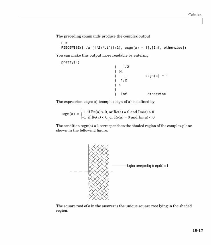
Calculus
The preceding commands produce the complex output
F =PIECEWISE([1/a^(1/2)*pi^(1/2), csgn(a) = 1],[Inf, otherwise])
You can make this output more readable by entering
pretty(F) { 1/2 { pi { ----- csgn(a) = 1 { 1/2 { a { { Inf otherwise
The expression csgn(a) (complex sign of a) is defined by
The condition csgn(a) = 1 corresponds to the shaded region of the complex plane shown in the following figure.
The square root of a in the answer is the unique square root lying in the shaded region.
csgn a( ) 1 if Re(a) > 0, or Re(a) = 0 and Im(a) > 0 1– if Re(a) < 0, or Re(a) = 0 and Im(a) < 0⎩
⎨⎧
=
Region corresponding to csgn(a) = 1
10-17
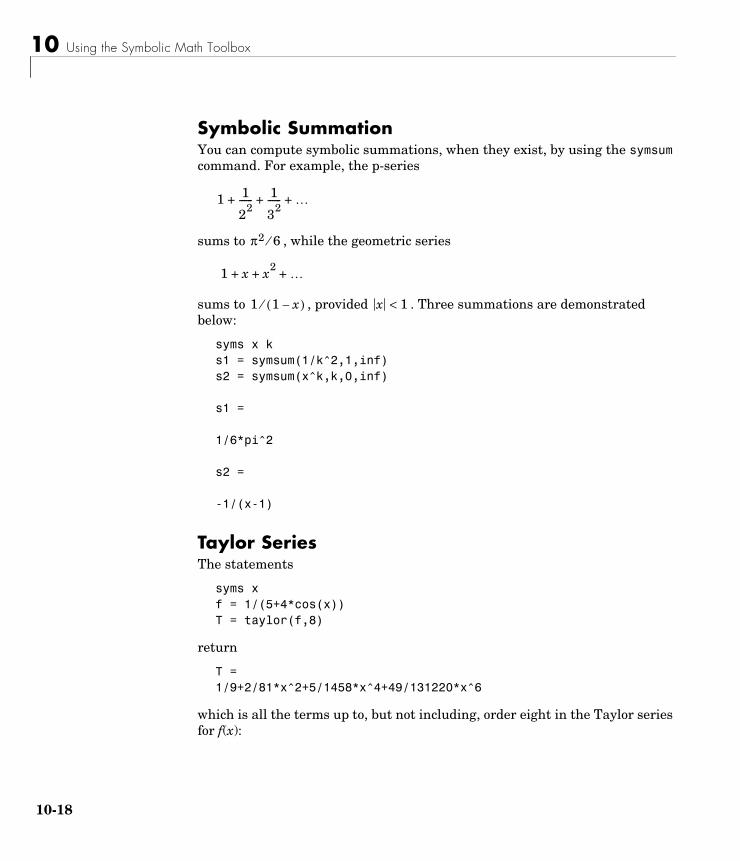
10 Using the Symbolic Math Toolbox
10-
Symbolic SummationYou can compute symbolic summations, when they exist, by using the symsum command. For example, the p-series
sums to , while the geometric series
sums to , provided . Three summations are demonstrated below:
syms x ks1 = symsum(1/k^2,1,inf)s2 = symsum(x^k,k,0,inf)
s1 = 1/6*pi^2
s2 = -1/(x-1)
Taylor SeriesThe statements
syms xf = 1/(5+4*cos(x))T = taylor(f,8)
return
T =1/9+2/81*x^2+5/1458*x^4+49/131220*x^6
which is all the terms up to, but not including, order eight in the Taylor series for f(x):
1 1
22------ 1
32------ …+ + +
π2 6⁄
1 x x2 …+ + +
1 1 x–( )⁄ x 1<
18
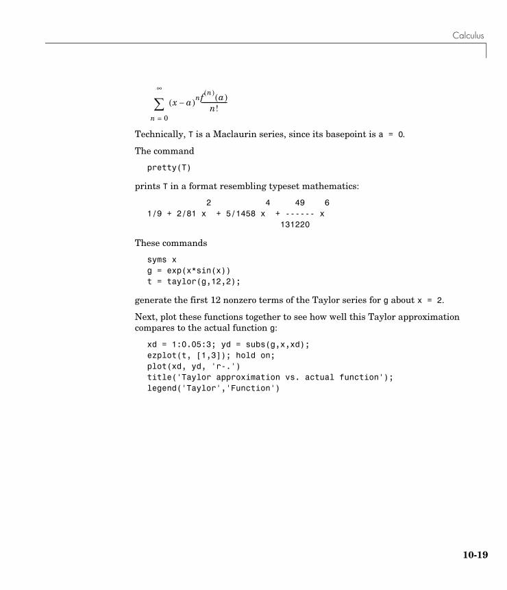
Calculus
Technically, T is a Maclaurin series, since its basepoint is a = 0.
The command
pretty(T)
prints T in a format resembling typeset mathematics:
2 4 49 61/9 + 2/81 x + 5/1458 x + ------ x 131220
These commands
syms xg = exp(x*sin(x))t = taylor(g,12,2);
generate the first 12 nonzero terms of the Taylor series for g about x = 2.
Next, plot these functions together to see how well this Taylor approximation compares to the actual function g:
xd = 1:0.05:3; yd = subs(g,x,xd);ezplot(t, [1,3]); hold on;plot(xd, yd, 'r-.')title('Taylor approximation vs. actual function');legend('Taylor','Function')
x a–( )n
n 0=
∞
∑f n( ) a( )
n!-----------------
10-19
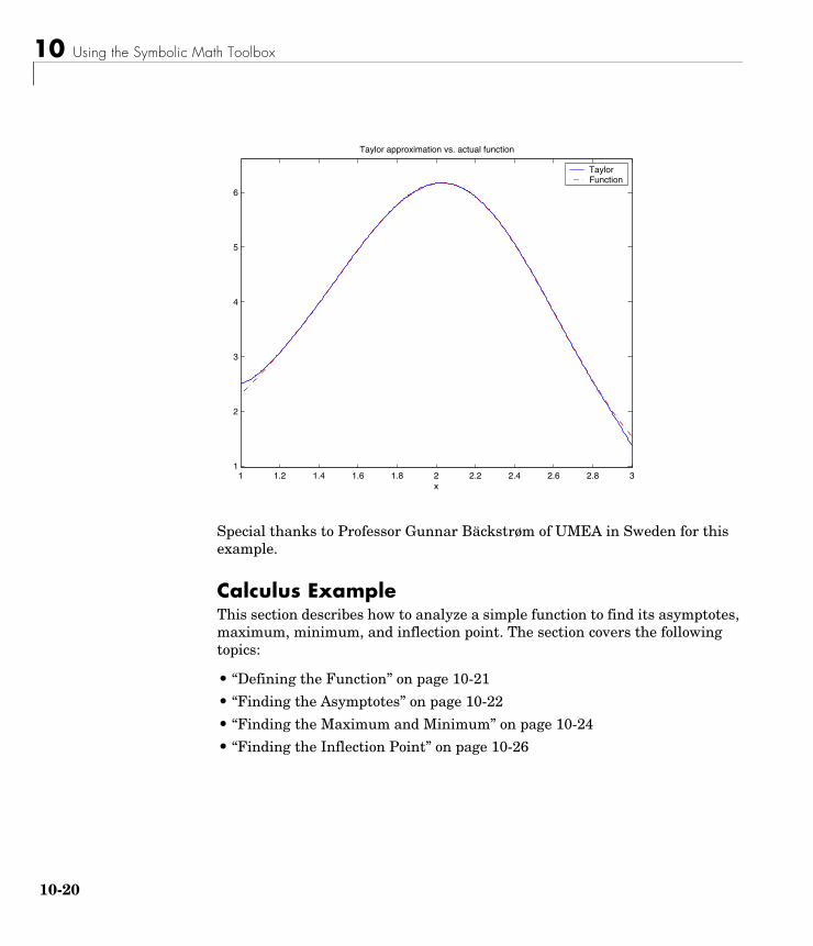
10 Using the Symbolic Math Toolbox
10-
Special thanks to Professor Gunnar Bäckstrøm of UMEA in Sweden for this example.
Calculus ExampleThis section describes how to analyze a simple function to find its asymptotes, maximum, minimum, and inflection point. The section covers the following topics:
• “Defining the Function” on page 10-21
• “Finding the Asymptotes” on page 10-22
• “Finding the Maximum and Minimum” on page 10-24
• “Finding the Inflection Point” on page 10-26
1 1.2 1.4 1.6 1.8 2 2.2 2.4 2.6 2.8 31
2
3
4
5
6
x
Taylor approximation vs. actual function
TaylorFunction
20
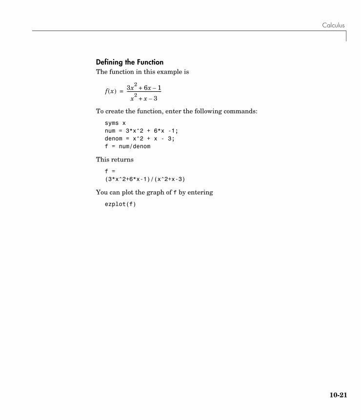
Calculus
Defining the FunctionThe function in this example is
To create the function, enter the following commands:
syms xnum = 3*x^2 + 6*x -1;denom = x^2 + x - 3;f = num/denom
This returns
f = (3*x^2+6*x-1)/(x^2+x-3)
You can plot the graph of f by entering
ezplot(f)
f x( ) 3x2 6x 1–+
x2 x 3–+--------------------------------=
10-21
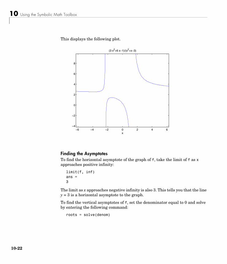
10 Using the Symbolic Math Toolbox
10-
This displays the following plot.
Finding the AsymptotesTo find the horizontal asymptote of the graph of f, take the limit of f as x approaches positive infinity:
limit(f, inf)ans = 3
The limit as x approaches negative infinity is also 3. This tells you that the line y = 3 is a horizontal asymptote to the graph.
To find the vertical asymptotes of f, set the denominator equal to 0 and solve by entering the following command:
roots = solve(denom)
−6 −4 −2 0 2 4 6−4
−2
0
2
4
6
8
x
(3 x2+6 x−1)/(x2+x−3)
22
Calculus
This returns to solutions to :
roots =[ -1/2+1/2*13^(1/2)][ -1/2-1/2*13^(1/2)]
This tells you that vertical asymptotes are the lines
and
You can plot the horizontal and vertical asymptotes with the following commands:
ezplot(f)hold on % Keep the graph of f in the figure% Plot horizontal asymptoteplot([-2*pi 2*pi], [3 3],'g')% Plot vertical asymptotes plot(double(roots(1))*[1 1], [-5 10],'r') plot(double(roots(2))*[1 1], [-5 10],'r')title('Horizontal and Vertical Asymptotes')hold off
Note that roots must be converted to double to use the plot command.
x2 x 3–+ 0=
x 1– 13+2
-------------------------=
x 1– 13–2
------------------------=
10-23
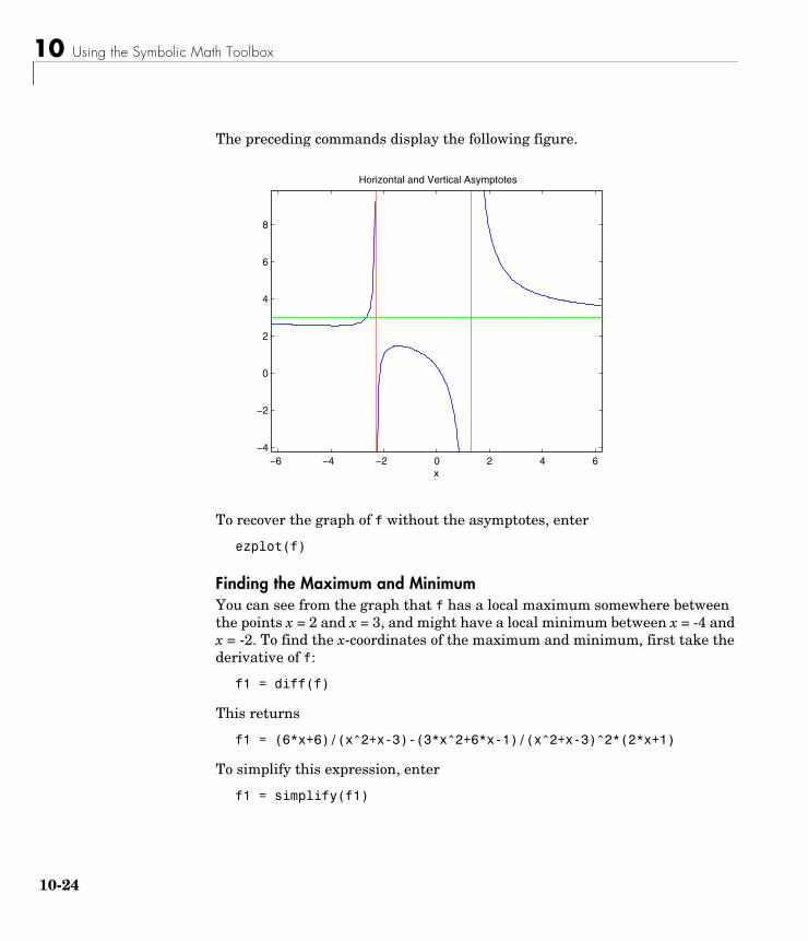
10 Using the Symbolic Math Toolbox
10-
The preceding commands display the following figure.
To recover the graph of f without the asymptotes, enter
ezplot(f)
Finding the Maximum and MinimumYou can see from the graph that f has a local maximum somewhere between the points x = 2 and x = 3, and might have a local minimum between x = -4 and x = -2. To find the x-coordinates of the maximum and minimum, first take the derivative of f:
f1 = diff(f)
This returns
f1 = (6*x+6)/(x^2+x-3)-(3*x^2+6*x-1)/(x^2+x-3)^2*(2*x+1)
To simplify this expression, enter
f1 = simplify(f1)
−6 −4 −2 0 2 4 6−4
−2
0
2
4
6
8
x
Horizontal and Vertical Asymptotes
24
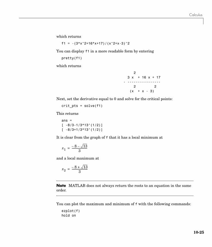
Calculus
which returns
f1 = -(3*x^2+16*x+17)/(x^2+x-3)^2
You can display f1 in a more readable form by entering
pretty(f1)
which returns
2 3 x + 16 x + 17 - ---------------- 2 2 (x + x - 3)
Next, set the derivative equal to 0 and solve for the critical points:
crit_pts = solve(f1)
This returns
ans =[ -8/3-1/3*13^(1/2)][ -8/3+1/3*13^(1/2)]
It is clear from the graph of f that it has a local minimum at
and a local maximum at
Note MATLAB does not always return the roots to an equation in the same order.
You can plot the maximum and minimum of f with the following commands:
ezplot(f)hold on
x18– 13–
3------------------------=
x28– 13+
3-------------------------=
10-25
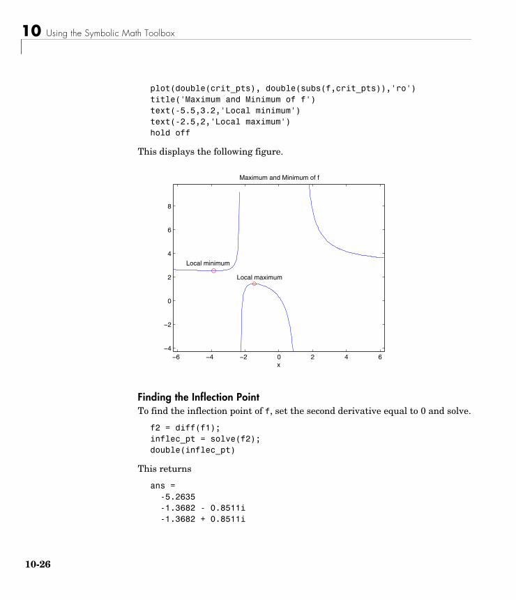
10 Using the Symbolic Math Toolbox
10-
plot(double(crit_pts), double(subs(f,crit_pts)),'ro')title('Maximum and Minimum of f')text(-5.5,3.2,'Local minimum')text(-2.5,2,'Local maximum')hold off
This displays the following figure.
Finding the Inflection PointTo find the inflection point of f, set the second derivative equal to 0 and solve.
f2 = diff(f1);inflec_pt = solve(f2);double(inflec_pt)
This returns
ans =-5.2635 -1.3682 - 0.8511i-1.3682 + 0.8511i
−6 −4 −2 0 2 4 6−4
−2
0
2
4
6
8
x
Maximum and Minimum of f
Local minimum
Local maximum
26
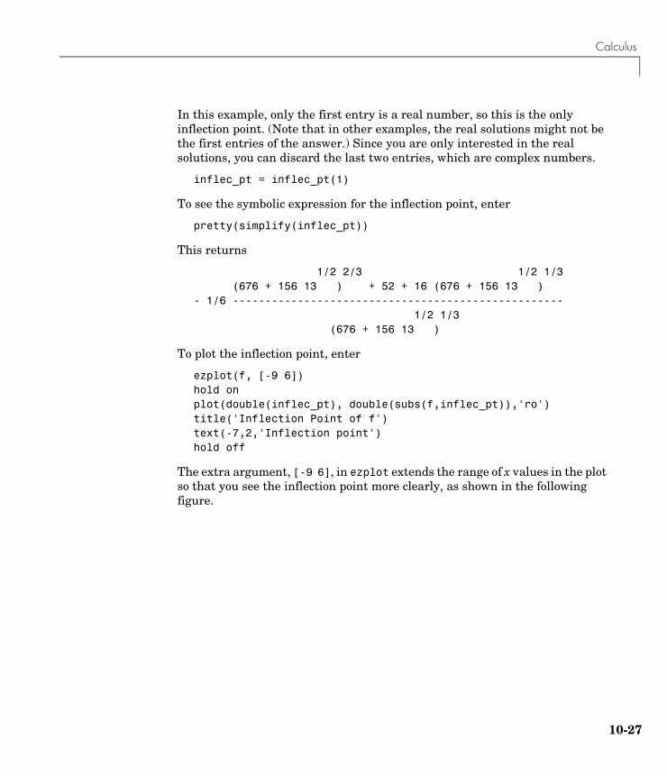
Calculus
In this example, only the first entry is a real number, so this is the only inflection point. (Note that in other examples, the real solutions might not be the first entries of the answer.) Since you are only interested in the real solutions, you can discard the last two entries, which are complex numbers.
inflec_pt = inflec_pt(1)
To see the symbolic expression for the inflection point, enter
pretty(simplify(inflec_pt))
This returns
1/2 2/3 1/2 1/3 (676 + 156 13 ) + 52 + 16 (676 + 156 13 )- 1/6 --------------------------------------------------- 1/2 1/3 (676 + 156 13 )
To plot the inflection point, enter
ezplot(f, [-9 6])hold onplot(double(inflec_pt), double(subs(f,inflec_pt)),'ro')title('Inflection Point of f')text(-7,2,'Inflection point')hold off
The extra argument, [-9 6], in ezplot extends the range of x values in the plot so that you see the inflection point more clearly, as shown in the following figure.
10-27
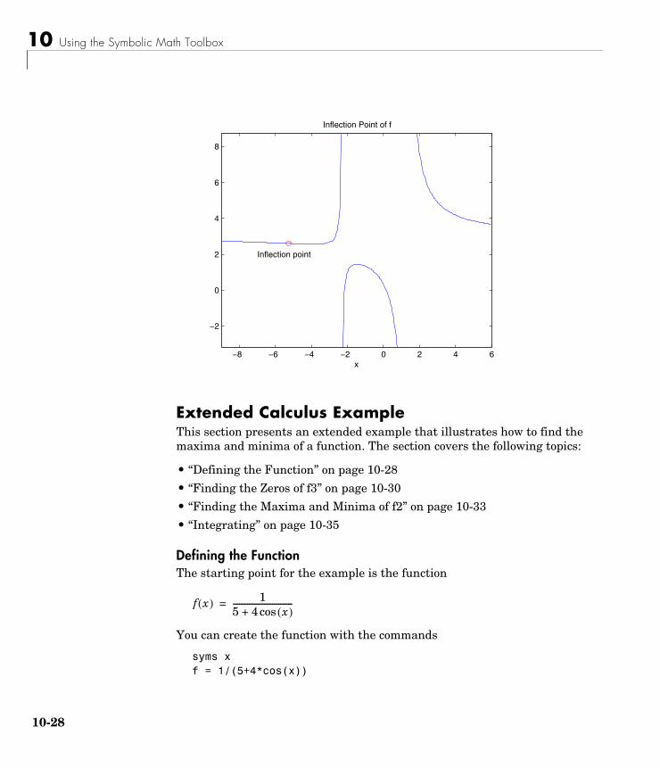
10 Using the Symbolic Math Toolbox
10-
Extended Calculus Example This section presents an extended example that illustrates how to find the maxima and minima of a function. The section covers the following topics:
• “Defining the Function” on page 10-28
• “Finding the Zeros of f3” on page 10-30
• “Finding the Maxima and Minima of f2” on page 10-33
• “Integrating” on page 10-35
Defining the FunctionThe starting point for the example is the function
You can create the function with the commands
syms x f = 1/(5+4*cos(x))
−8 −6 −4 −2 0 2 4 6
−2
0
2
4
6
8
x
Inflection Point of f
Inflection point
f x( ) 15 4 x( )cos+------------------------------=
28
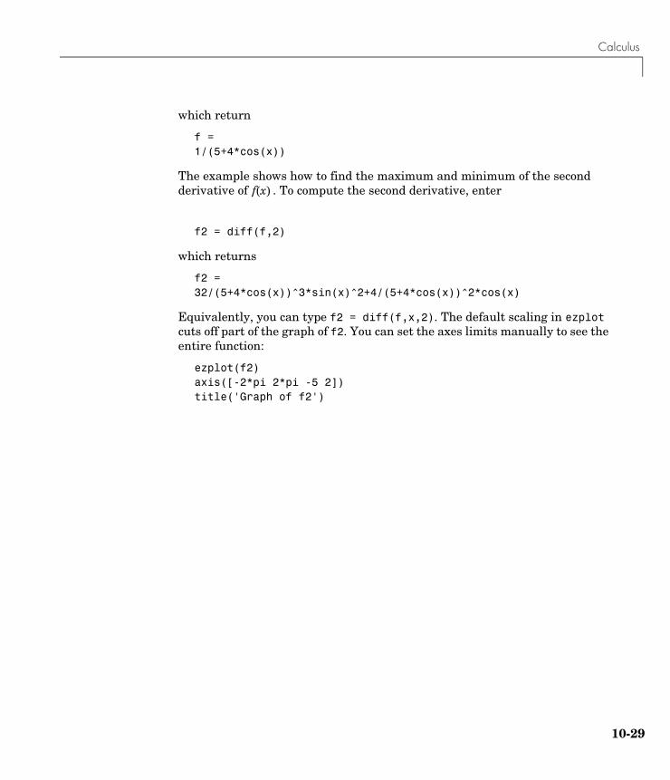
Calculus
which return
f =1/(5+4*cos(x))
The example shows how to find the maximum and minimum of the second derivative of . To compute the second derivative, enter
f2 = diff(f,2)
which returns
f2 =32/(5+4*cos(x))^3*sin(x)^2+4/(5+4*cos(x))^2*cos(x)
Equivalently, you can type f2 = diff(f,x,2). The default scaling in ezplot cuts off part of the graph of f2. You can set the axes limits manually to see the entire function:
ezplot(f2) axis([-2*pi 2*pi -5 2])title('Graph of f2')
f x( )
10-29
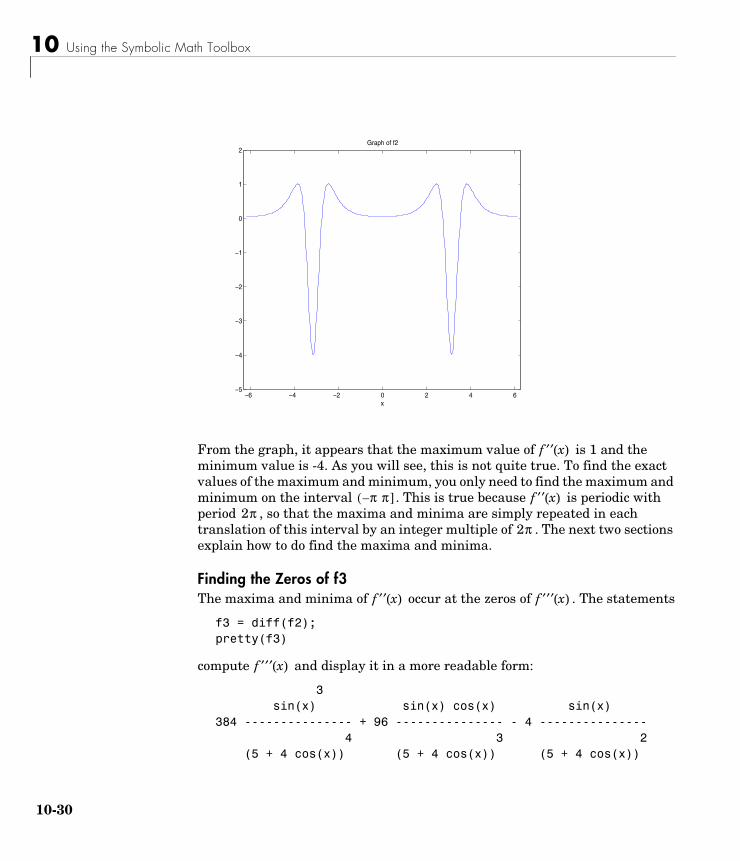
10 Using the Symbolic Math Toolbox
10-
From the graph, it appears that the maximum value of is 1 and the minimum value is -4. As you will see, this is not quite true. To find the exact values of the maximum and minimum, you only need to find the maximum and minimum on the interval . This is true because is periodic with period , so that the maxima and minima are simply repeated in each translation of this interval by an integer multiple of . The next two sections explain how to do find the maxima and minima.
Finding the Zeros of f3The maxima and minima of occur at the zeros of . The statements
f3 = diff(f2);pretty(f3)
compute and display it in a more readable form:
3 sin(x) sin(x) cos(x) sin(x)384 --------------- + 96 --------------- - 4 --------------- 4 3 2 (5 + 4 cos(x)) (5 + 4 cos(x)) (5 + 4 cos(x))
−6 −4 −2 0 2 4 6−5
−4
−3
−2
−1
0
1
2
x
Graph of f2
f ′′ x( )
π–( π] f ′′ x( )2π
2π
f ′′ x( ) f ′′′ x( )
f ′′′ x( )
30
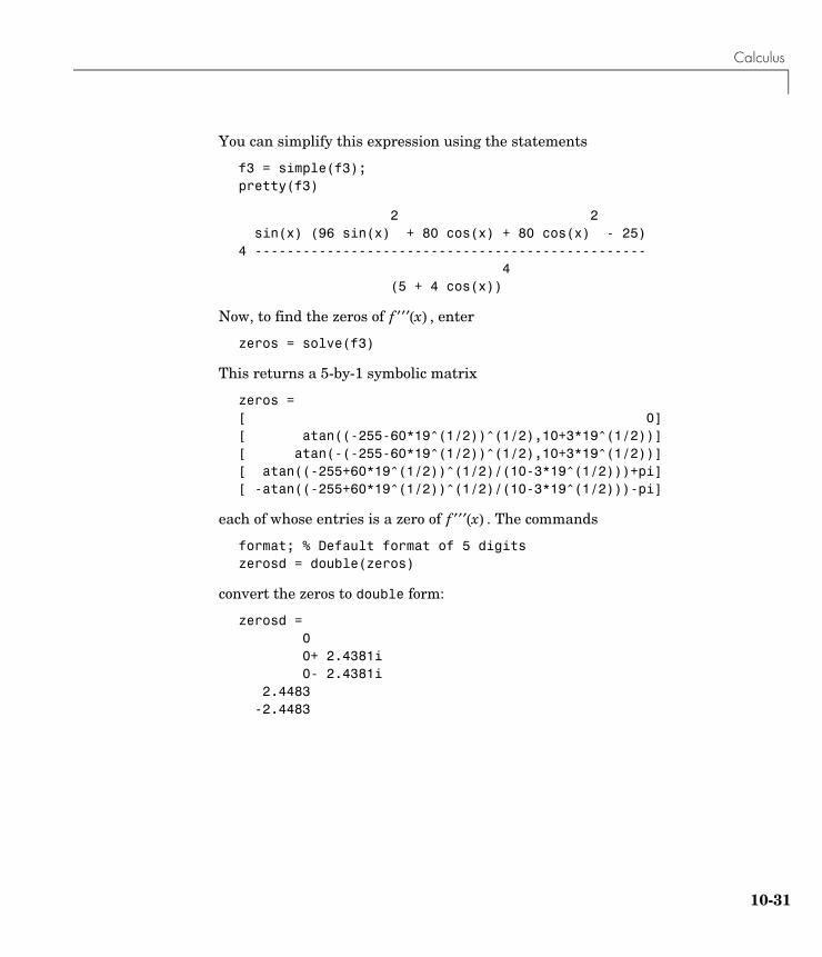
Calculus
You can simplify this expression using the statements
f3 = simple(f3);pretty(f3)
2 2 sin(x) (96 sin(x) + 80 cos(x) + 80 cos(x) - 25)4 ------------------------------------------------- 4 (5 + 4 cos(x))
Now, to find the zeros of , enter
zeros = solve(f3)
This returns a 5-by-1 symbolic matrix
zeros =[ 0][ atan((-255-60*19^(1/2))^(1/2),10+3*19^(1/2))][ atan(-(-255-60*19^(1/2))^(1/2),10+3*19^(1/2))][ atan((-255+60*19^(1/2))^(1/2)/(10-3*19^(1/2)))+pi][ -atan((-255+60*19^(1/2))^(1/2)/(10-3*19^(1/2)))-pi]
each of whose entries is a zero of . The commands
format; % Default format of 5 digitszerosd = double(zeros)
convert the zeros to double form:
zerosd = 0 0+ 2.4381i 0- 2.4381i 2.4483 -2.4483
f ′′′ x( )
f ′′′ x( )
10-31
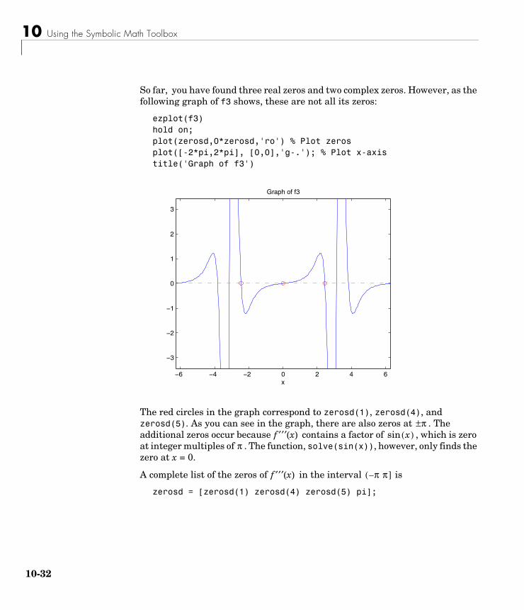
10 Using the Symbolic Math Toolbox
10-
So far, you have found three real zeros and two complex zeros. However, as the following graph of f3 shows, these are not all its zeros:
ezplot(f3)hold on;plot(zerosd,0*zerosd,'ro') % Plot zerosplot([-2*pi,2*pi], [0,0],'g-.'); % Plot x-axistitle('Graph of f3')
The red circles in the graph correspond to zerosd(1), zerosd(4), and zerosd(5). As you can see in the graph, there are also zeros at . The additional zeros occur because contains a factor of , which is zero at integer multiples of . The function, solve(sin(x)), however, only finds the zero at x = 0.
A complete list of the zeros of in the interval is
zerosd = [zerosd(1) zerosd(4) zerosd(5) pi];
−6 −4 −2 0 2 4 6
−3
−2
−1
0
1
2
3
x
Graph of f3
π±f ′′′ x( ) x( )sin
π
f ′′′ x( ) π–( π]
32
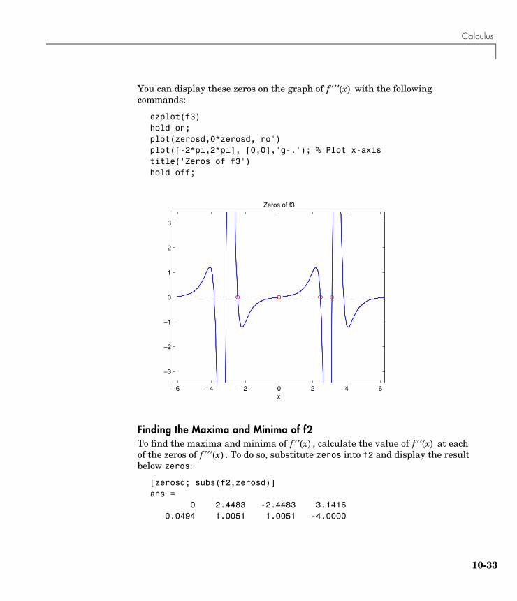
Calculus
You can display these zeros on the graph of with the following commands:
ezplot(f3)hold on;plot(zerosd,0*zerosd,'ro')plot([-2*pi,2*pi], [0,0],'g-.'); % Plot x-axistitle('Zeros of f3')hold off;
Finding the Maxima and Minima of f2To find the maxima and minima of , calculate the value of at each of the zeros of . To do so, substitute zeros into f2 and display the result below zeros:
[zerosd; subs(f2,zerosd)]ans =
0 2.4483 -2.4483 3.14160.0494 1.0051 1.0051 -4.0000
f ′′′ x( )
−6 −4 −2 0 2 4 6
−3
−2
−1
0
1
2
3
x
Zeros of f3
f ′′ x( ) f ′′ x( )f ′′′ x( )
10-33
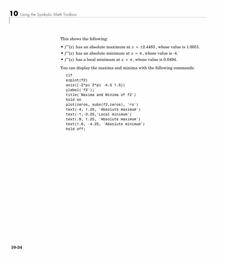
10 Using the Symbolic Math Toolbox
10-
This shows the following:
• has an absolute maximum at , whose value is 1.0051.
• has an absolute minimum at , whose value is -4.
• has a local minimum at , whose value is 0.0494.
You can display the maxima and minima with the following commands:
clfezplot(f2)axis([-2*pi 2*pi -4.5 1.5])ylabel('f2');title('Maxima and Minima of f2')hold onplot(zeros, subs(f2,zeros), 'ro')text(-4, 1.25, 'Absolute maximum')text(-1,-0.25,'Local minimum')text(.9, 1.25, 'Absolute maximum')text(1.6, -4.25, 'Absolute minimum')hold off;
f ′′ x( ) x 2.4483±=
f ′′ x( ) x π=
f ′′ x( ) x π=
34
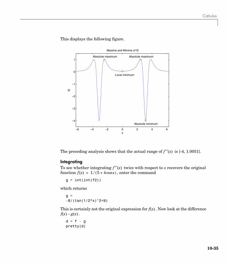
Calculus
This displays the following figure.
The preceding analysis shows that the actual range of is [-4, 1.0051].
IntegratingTo see whether integrating twice with respect to x recovers the original function , enter the command
g = int(int(f2))
which returns
g =-8/(tan(1/2*x)^2+9)
This is certainly not the original expression for . Now look at the difference .
d = f - gpretty(d)
−6 −4 −2 0 2 4 6
−4
−3
−2
−1
0
1
x
Maxima and Minima of f2
f2
Absolute maximum
Local minimum
Absolute maximum
Absolute minimum
f ′′ x( )
f ′′ x( )f x( ) 1 5 4 xcos+( )⁄=
f x( )f x( ) g x( )–
10-35
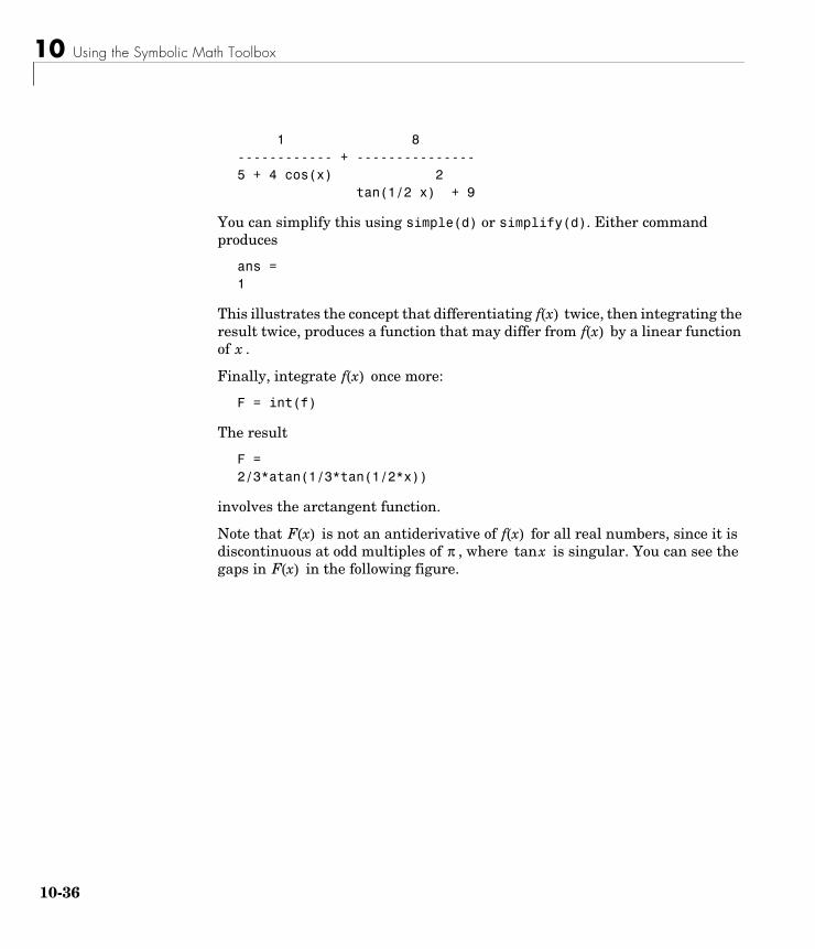
10 Using the Symbolic Math Toolbox
10-
1 8------------ + ---------------5 + 4 cos(x) 2 tan(1/2 x) + 9
You can simplify this using simple(d) or simplify(d). Either command produces
ans =1
This illustrates the concept that differentiating twice, then integrating the result twice, produces a function that may differ from by a linear function of .
Finally, integrate once more:
F = int(f)
The result
F =2/3*atan(1/3*tan(1/2*x))
involves the arctangent function.
Note that is not an antiderivative of for all real numbers, since it is discontinuous at odd multiples of , where is singular. You can see the gaps in in the following figure.
f x( )f x( )
x
f x( )
F x( ) f x( )π xtan
F x( )
36
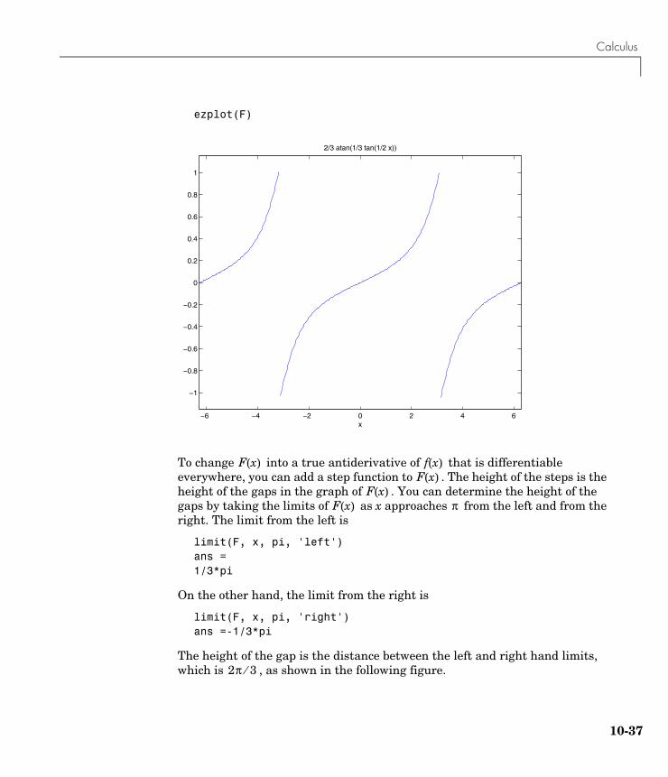
Calculus
ezplot(F)
To change into a true antiderivative of that is differentiable everywhere, you can add a step function to . The height of the steps is the height of the gaps in the graph of . You can determine the height of the gaps by taking the limits of as x approaches from the left and from the right. The limit from the left is
limit(F, x, pi, 'left')ans =1/3*pi
On the other hand, the limit from the right is
limit(F, x, pi, 'right')ans =-1/3*pi
The height of the gap is the distance between the left and right hand limits, which is , as shown in the following figure.
−6 −4 −2 0 2 4 6
−1
−0.8
−0.6
−0.4
−0.2
0
0.2
0.4
0.6
0.8
1
x
2/3 atan(1/3 tan(1/2 x))
F x( ) f x( )F x( )
F x( )F x( ) π
2π 3⁄
10-37
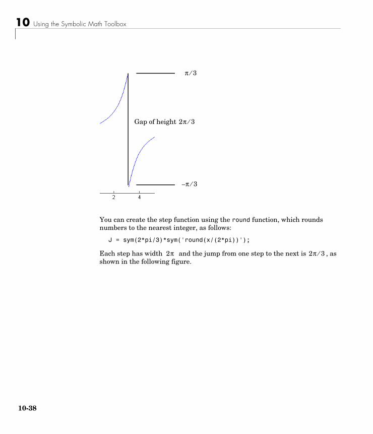
10 Using the Symbolic Math Toolbox
10-
You can create the step function using the round function, which rounds numbers to the nearest integer, as follows:
J = sym(2*pi/3)*sym('round(x/(2*pi))');
Each step has width and the jump from one step to the next is , as shown in the following figure.
Gap of height 2π 3⁄
π 3⁄
π– 3⁄
2π 2π 3⁄
38
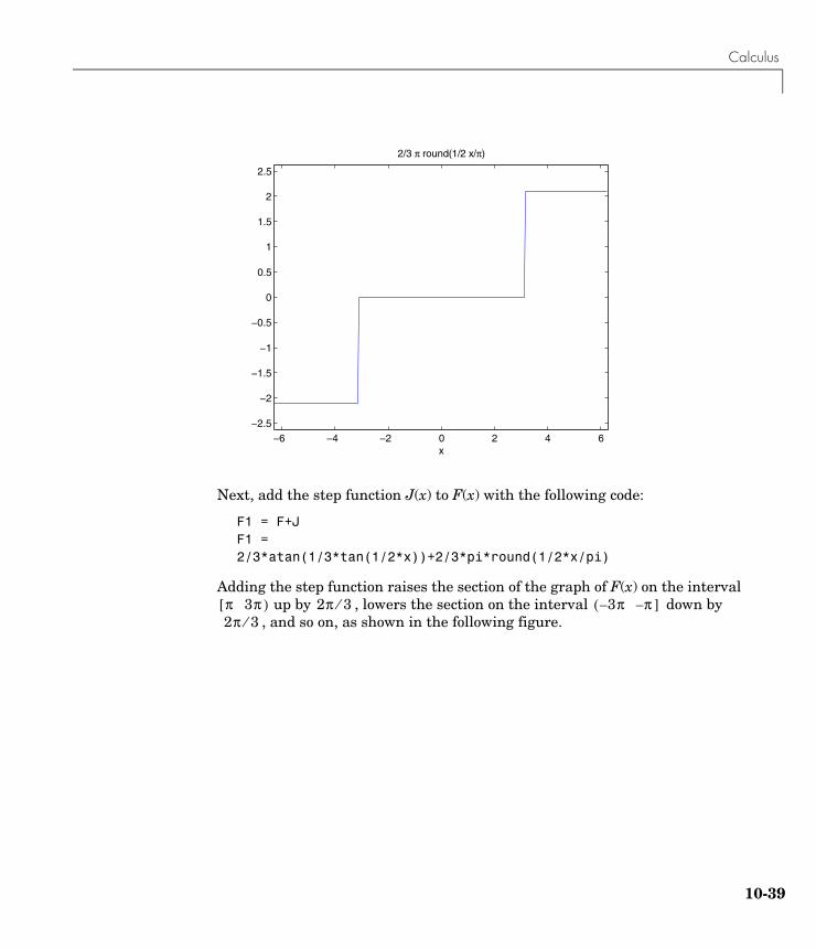
Calculus
Next, add the step function J(x) to F(x) with the following code:
F1 = F+JF1 =2/3*atan(1/3*tan(1/2*x))+2/3*pi*round(1/2*x/pi)
Adding the step function raises the section of the graph of F(x) on the interval up by , lowers the section on the interval down by
, and so on, as shown in the following figure.
−6 −4 −2 0 2 4 6−2.5
−2
−1.5
−1
−0.5
0
0.5
1
1.5
2
2.5
x
2/3 π round(1/2 x/π)
π[ 3π ) 2π 3⁄ 3π–( π ]–2π 3⁄
10-39
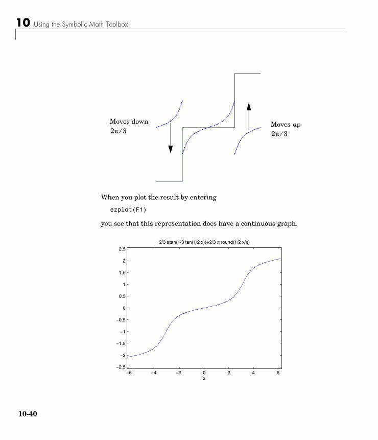
10 Using the Symbolic Math Toolbox
10-
When you plot the result by entering
ezplot(F1)
you see that this representation does have a continuous graph.
Moves up 2π 3⁄
Moves down 2π 3⁄
−6 −4 −2 0 2 4 6−2.5
−2
−1.5
−1
−0.5
0
0.5
1
1.5
2
2.5
x
2/3 atan(1/3 tan(1/2 x))+2/3 π round(1/2 x/π)
40
Simplifications and Substitutions
Simplifications and SubstitutionsThere are several functions that simplify symbolic expressions and are used to perform symbolic substitutions:
SimplificationsHere are three different symbolic expressions.
syms xf = x^3-6*x^2+11*x-6g = (x-1)*(x-2)*(x-3)h = -6+(11+(-6+x)*x)*x
Here are their prettyprinted forms, generated by
pretty(f), pretty(g), pretty(h)
3 2x - 6 x + 11 x - 6
(x - 1) (x - 2) (x - 3)
-6 + (11 + (-6 + x) x) x
These expressions are three different representations of the same mathematical function, a cubic polynomial in x.
Each of the three forms is preferable to the others in different situations. The first form, f, is the most commonly used representation of a polynomial. It is simply a linear combination of the powers of x. The second form, g, is the factored form. It displays the roots of the polynomial and is the most accurate for numerical evaluation near the roots. But, if a polynomial does not have such simple roots, its factored form may not be so convenient. The third form, h, is the Horner, or nested, representation. For numerical evaluation, it involves the fewest arithmetic operations and is the most accurate for some other ranges of x.
The symbolic simplification problem involves the verification that these three expressions represent the same function. It also involves a less clearly defined objective — which of these representations is “the simplest”?
10-41
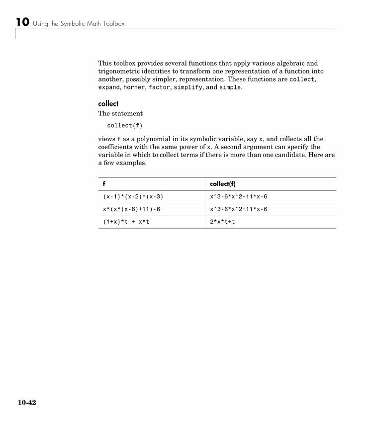
10 Using the Symbolic Math Toolbox
10-
This toolbox provides several functions that apply various algebraic and trigonometric identities to transform one representation of a function into another, possibly simpler, representation. These functions are collect, expand, horner, factor, simplify, and simple.
collectThe statement
collect(f)
views f as a polynomial in its symbolic variable, say x, and collects all the coefficients with the same power of x. A second argument can specify the variable in which to collect terms if there is more than one candidate. Here are a few examples.
f collect(f)
(x-1)*(x-2)*(x-3) x^3-6*x^2+11*x-6
x*(x*(x-6)+11)-6 x^3-6*x^2+11*x-6
(1+x)*t + x*t 2*x*t+t
42
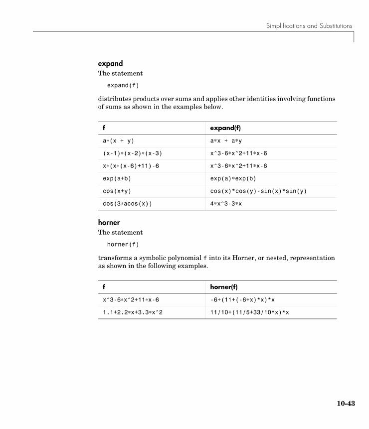
Simplifications and Substitutions
expandThe statement
expand(f)
distributes products over sums and applies other identities involving functions of sums as shown in the examples below.
hornerThe statement
horner(f)
transforms a symbolic polynomial f into its Horner, or nested, representation as shown in the following examples.
f expand(f)
a∗(x + y) a∗x + a∗y
(x-1)∗(x-2)∗(x-3) x^3-6∗x^2+11∗x-6
x∗(x∗(x-6)+11)-6 x^3-6∗x^2+11∗x-6
exp(a+b) exp(a)∗exp(b)
cos(x+y) cos(x)*cos(y)-sin(x)*sin(y)
cos(3∗acos(x)) 4∗x^3-3∗x
f horner(f)
x^3-6∗x^2+11∗x-6 -6+(11+(-6+x)*x)*x
1.1+2.2∗x+3.3∗x^2 11/10+(11/5+33/10*x)*x
10-43
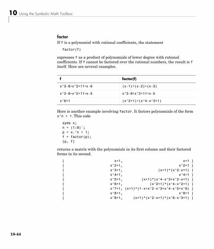
10 Using the Symbolic Math Toolbox
10-
factorIf f is a polynomial with rational coefficients, the statement
factor(f)
expresses f as a product of polynomials of lower degree with rational coefficients. If f cannot be factored over the rational numbers, the result is f itself. Here are several examples.
Here is another example involving factor. It factors polynomials of the form x^n + 1. This code
syms x;n = (1:9)'; p = x.^n + 1;f = factor(p);[p, f]
returns a matrix with the polynomials in its first column and their factored forms in its second.
[ x+1, x+1 ][ x^2+1, x^2+1 ][ x^3+1, (x+1)*(x^2-x+1) ][ x^4+1, x^4+1 ][ x^5+1, (x+1)*(x^4-x^3+x^2-x+1) ][ x^6+1, (x^2+1)*(x^4-x^2+1) ][ x^7+1, (x+1)*(1-x+x^2-x^3+x^4-x^5+x^6) ][ x^8+1, x^8+1 ][ x^9+1, (x+1)*(x^2-x+1)*(x^6-x^3+1) ]
f factor(f)
x^3-6∗x^2+11∗x-6 (x-1)∗(x-2)∗(x-3)
x^3-6∗x^2+11∗x-5 x^3-6∗x^2+11∗x-5
x^6+1 (x^2+1)∗(x^4-x^2+1)
44
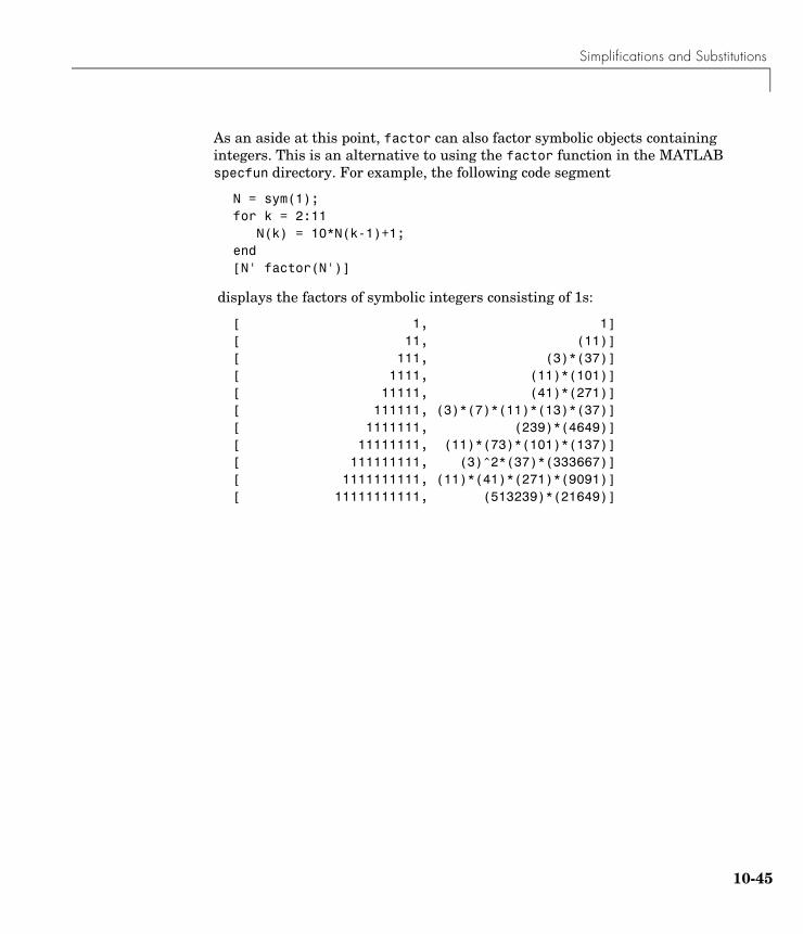
Simplifications and Substitutions
As an aside at this point, factor can also factor symbolic objects containing integers. This is an alternative to using the factor function in the MATLAB specfun directory. For example, the following code segment
N = sym(1);for k = 2:11 N(k) = 10*N(k-1)+1;end[N' factor(N')]
displays the factors of symbolic integers consisting of 1s:
[ 1, 1][ 11, (11)][ 111, (3)*(37)][ 1111, (11)*(101)][ 11111, (41)*(271)][ 111111, (3)*(7)*(11)*(13)*(37)][ 1111111, (239)*(4649)][ 11111111, (11)*(73)*(101)*(137)][ 111111111, (3)^2*(37)*(333667)][ 1111111111, (11)*(41)*(271)*(9091)][ 11111111111, (513239)*(21649)]
10-45
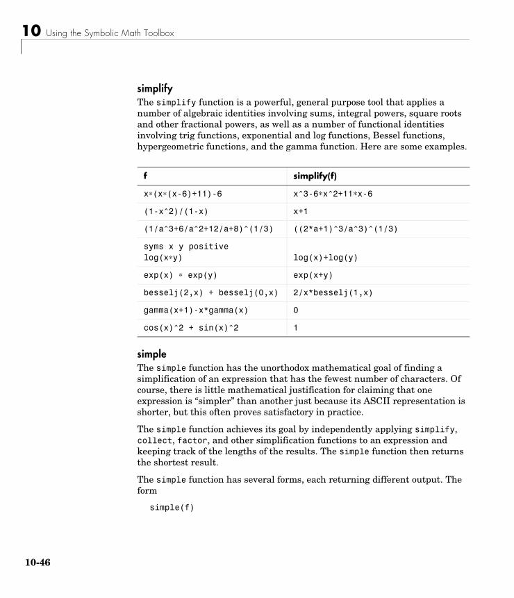
10 Using the Symbolic Math Toolbox
10-
simplifyThe simplify function is a powerful, general purpose tool that applies a number of algebraic identities involving sums, integral powers, square roots and other fractional powers, as well as a number of functional identities involving trig functions, exponential and log functions, Bessel functions, hypergeometric functions, and the gamma function. Here are some examples.
simpleThe simple function has the unorthodox mathematical goal of finding a simplification of an expression that has the fewest number of characters. Of course, there is little mathematical justification for claiming that one expression is “simpler” than another just because its ASCII representation is shorter, but this often proves satisfactory in practice.
The simple function achieves its goal by independently applying simplify, collect, factor, and other simplification functions to an expression and keeping track of the lengths of the results. The simple function then returns the shortest result.
The simple function has several forms, each returning different output. The form
simple(f)
f simplify(f)
x∗(x∗(x-6)+11)-6 x^3-6∗x^2+11∗x-6
(1-x^2)/(1-x) x+1
(1/a^3+6/a^2+12/a+8)^(1/3) ((2*a+1)^3/a^3)^(1/3)
syms x y positivelog(x∗y) log(x)+log(y)
exp(x) ∗ exp(y) exp(x+y)
besselj(2,x) + besselj(0,x) 2/x*besselj(1,x)
gamma(x+1)-x*gamma(x) 0
cos(x)^2 + sin(x)^2 1
46
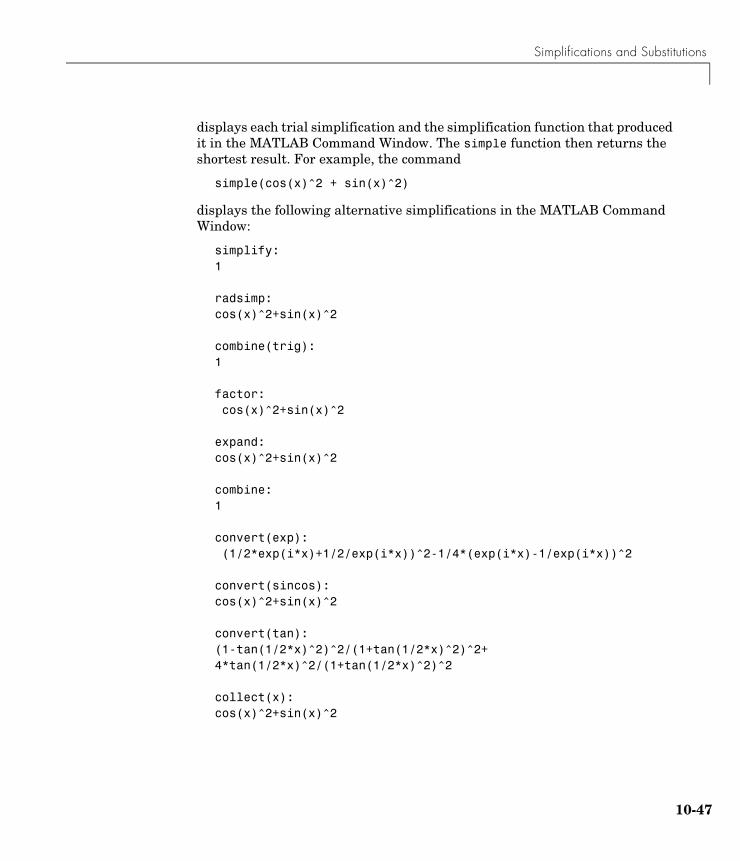
Simplifications and Substitutions
displays each trial simplification and the simplification function that produced it in the MATLAB Command Window. The simple function then returns the shortest result. For example, the command
simple(cos(x)^2 + sin(x)^2)
displays the following alternative simplifications in the MATLAB Command Window:
simplify:1 radsimp:cos(x)^2+sin(x)^2 combine(trig):1 factor: cos(x)^2+sin(x)^2 expand:cos(x)^2+sin(x)^2 combine:1 convert(exp): (1/2*exp(i*x)+1/2/exp(i*x))^2-1/4*(exp(i*x)-1/exp(i*x))^2 convert(sincos):cos(x)^2+sin(x)^2 convert(tan):(1-tan(1/2*x)^2)^2/(1+tan(1/2*x)^2)^2+4*tan(1/2*x)^2/(1+tan(1/2*x)^2)^2 collect(x):cos(x)^2+sin(x)^2
10-47
10 Using the Symbolic Math Toolbox
10-
and returns
ans =1
This form is useful when you want to check, for example, whether the shortest form is indeed the simplest. If you are not interested in how simple achieves its result, use the form
f = simple(f)
This form simply returns the shortest expression found. For example, the statement
f = simple(cos(x)^2+sin(x)^2)
returns
f =1
If you want to know which simplification returned the shortest result, use the multiple output form:
[F, how] = simple(f)
This form returns the shortest result in the first variable and the simplification method used to achieve the result in the second variable. For example, the statement
[f, how] = simple(cos(x)^2+sin(x)^2)
returns
f =1 how =combine
The simple function sometimes improves on the result returned by simplify, one of the simplifications that it tries. For example, when applied to the
48
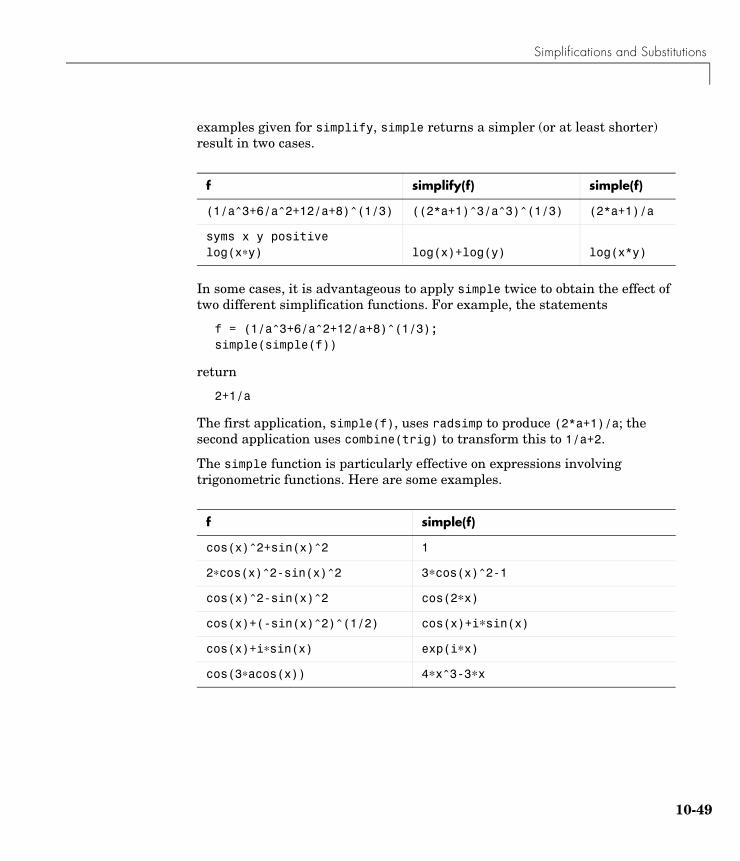
Simplifications and Substitutions
examples given for simplify, simple returns a simpler (or at least shorter) result in two cases.
In some cases, it is advantageous to apply simple twice to obtain the effect of two different simplification functions. For example, the statements
f = (1/a^3+6/a^2+12/a+8)^(1/3);simple(simple(f))
return
2+1/a
The first application, simple(f), uses radsimp to produce (2*a+1)/a; the second application uses combine(trig) to transform this to 1/a+2.
The simple function is particularly effective on expressions involving trigonometric functions. Here are some examples.
f simplify(f) simple(f)
(1/a^3+6/a^2+12/a+8)^(1/3) ((2*a+1)^3/a^3)^(1/3) (2*a+1)/a
syms x y positivelog(x∗y) log(x)+log(y) log(x*y)
f simple(f)
cos(x)^2+sin(x)^2 1
2∗cos(x)^2-sin(x)^2 3∗cos(x)^2-1
cos(x)^2-sin(x)^2 cos(2∗x)
cos(x)+(-sin(x)^2)^(1/2) cos(x)+i∗sin(x)
cos(x)+i∗sin(x) exp(i∗x)
cos(3∗acos(x)) 4∗x^3-3∗x
10-49
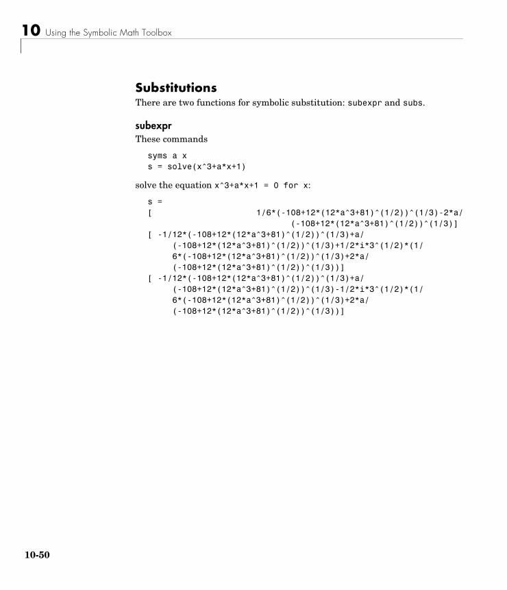
10 Using the Symbolic Math Toolbox
10-
SubstitutionsThere are two functions for symbolic substitution: subexpr and subs.
subexprThese commands
syms a xs = solve(x^3+a*x+1)
solve the equation x^3+a*x+1 = 0 for x:
s =[ 1/6*(-108+12*(12*a^3+81)^(1/2))^(1/3)-2*a/ (-108+12*(12*a^3+81)^(1/2))^(1/3)][ -1/12*(-108+12*(12*a^3+81)^(1/2))^(1/3)+a/ (-108+12*(12*a^3+81)^(1/2))^(1/3)+1/2*i*3^(1/2)*(1/ 6*(-108+12*(12*a^3+81)^(1/2))^(1/3)+2*a/ (-108+12*(12*a^3+81)^(1/2))^(1/3))][ -1/12*(-108+12*(12*a^3+81)^(1/2))^(1/3)+a/ (-108+12*(12*a^3+81)^(1/2))^(1/3)-1/2*i*3^(1/2)*(1/ 6*(-108+12*(12*a^3+81)^(1/2))^(1/3)+2*a/ (-108+12*(12*a^3+81)^(1/2))^(1/3))]
50
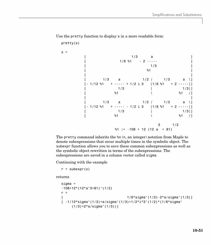
Simplifications and Substitutions
Use the pretty function to display s in a more readable form:
pretty(s) s =
[ 1/3 a ][ 1/6 %1 - 2 ----- ][ 1/3 ][ %1 ][ ][ 1/3 a 1/2 / 1/3 a \][- 1/12 %1 + ----- + 1/2 i 3 |1/6 %1 + 2 -----|][ 1/3 | 1/3|][ %1 \ %1 /][ ][ 1/3 a 1/2 / 1/3 a \][- 1/12 %1 + ----- - 1/2 i 3 |1/6 %1 + 2 -----|][ 1/3 | 1/3|][ %1 \ %1 /]
3 1/2 %1 := -108 + 12 (12 a + 81)
The pretty command inherits the %n (n, an integer) notation from Maple to denote subexpressions that occur multiple times in the symbolic object. The subexpr function allows you to save these common subexpressions as well as the symbolic object rewritten in terms of the subexpressions. The subexpressions are saved in a column vector called sigma.
Continuing with the example
r = subexpr(s)
returns
sigma =-108+12*(12*a^3+81)^(1/2)r =[ 1/6*sigma^(1/3)-2*a/sigma^(1/3)][ -1/12*sigma^(1/3)+a/sigma^(1/3)+1/2*i*3^(1/2)*(1/6*sigma^ (1/3)+2*a/sigma^(1/3))]
10-51
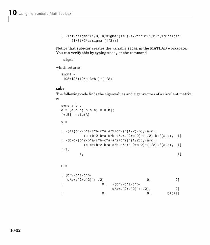
10 Using the Symbolic Math Toolbox
10-
[ -1/12*sigma^(1/3)+a/sigma^(1/3)-1/2*i*3^(1/2)*(1/6*sigma^ (1/3)+2*a/sigma^(1/3))]
Notice that subexpr creates the variable sigma in the MATLAB workspace. You can verify this by typing whos, or the command
sigma
which returns
sigma =-108+12*(12*a^3+81)^(1/2)
subsThe following code finds the eigenvalues and eigenvectors of a circulant matrix A:
syms a b cA = [a b c; b c a; c a b];[v,E] = eig(A)
v =
[ -(a+(b^2-b*a-c*b-c*a+a^2+c^2)^(1/2)-b)/(a-c), -(a-(b^2-b*a-c*b-c*a+a^2+c^2)^(1/2)-b)/(a-c), 1][ -(b-c-(b^2-b*a-c*b-c*a+a^2+c^2)^(1/2))/(a-c), -(b-c+(b^2-b*a-c*b-c*a+a^2+c^2)^(1/2))/(a-c), 1][ 1, 1, 1]
E =
[ (b^2-b*a-c*b- c*a+a^2+c^2)^(1/2), 0, 0][ 0, -(b^2-b*a-c*b- c*a+a^2+c^2)^(1/2), 0][ 0, 0, b+c+a]
52
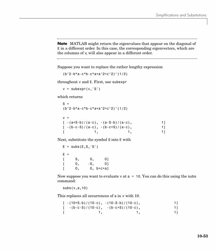
Simplifications and Substitutions
Note MATLAB might return the eigenvalues that appear on the diagonal of E in a different order. In this case, the corresponding eigenvectors, which are the columns of v, will also appear in a different order.
Suppose you want to replace the rather lengthy expression
(b^2-b*a-c*b-c*a+a^2+c^2)^(1/2)
throughout v and E. First, use subexpr
v = subexpr(v,'S')
which returns
S =(b^2-b*a-c*b-c*a+a^2+c^2)^(1/2)
v =[ -(a+S-b)/(a-c), -(a-S-b)/(a-c), 1][ -(b-c-S)/(a-c), -(b-c+S)/(a-c), 1][ 1, 1, 1]
Next, substitute the symbol S into E with
E = subs(E,S,'S')
E =[ S, 0, 0][ 0, -S, 0][ 0, 0, b+c+a]
Now suppose you want to evaluate v at a = 10. You can do this using the subs command:
subs(v,a,10)
This replaces all occurrences of a in v with 10.
[ -(10+S-b)/(10-c), -(10-S-b)/(10-c), 1][ -(b-c-S)/(10-c), -(b-c+S)/(10-c), 1][ 1, 1, 1]
10-53
10 Using the Symbolic Math Toolbox
10-
Notice, however, that the symbolic expression that S represents is unaffected by this substitution. That is, the symbol a in S is not replaced by 10. The subs command is also a useful function for substituting in a variety of values for several variables in a particular expression. For example, suppose that in addition to substituting a = 10 in S, you also want to substitute the values for 2 and 10 for b and c, respectively. The way to do this is to set values for a, b, and c in the workspace. Then subs evaluates its input using the existing symbolic and double variables in the current workspace. In the example, you first set
a = 10; b = 2; c = 10;subs(S)
ans =8
To look at the contents of the workspace, type whos, which gives
Name Size Bytes Class
A 3x3 878 sym object E 3x3 888 sym object S 1x1 186 sym object a 1x1 8 double array ans 1x1 140 sym object b 1x1 8 double array c 1x1 8 double array v 3x3 982 sym object
a, b, and c are now variables of class double while A, E, S, and v remain symbolic expressions (class sym).
If you want to preserve a, b, and c as symbolic variables, but still alter their value within S, use this procedure.
syms a b csubs(S,{a,b,c},{10,2,10})
ans =8
Typing whos reveals that a, b, and c remain 1-by-1 sym objects.
54
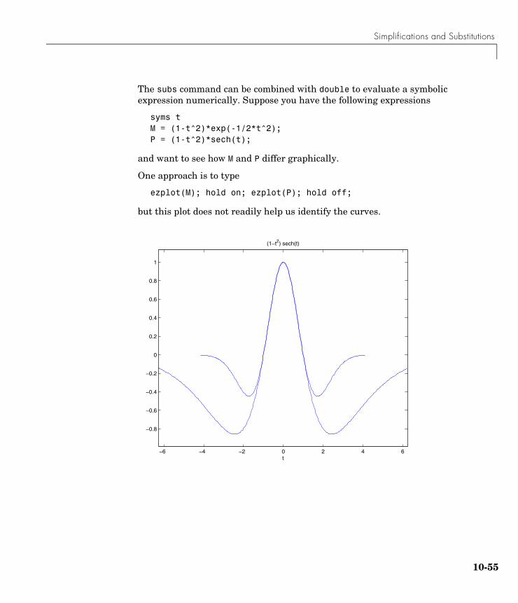
Simplifications and Substitutions
The subs command can be combined with double to evaluate a symbolic expression numerically. Suppose you have the following expressions
syms tM = (1-t^2)*exp(-1/2*t^2);P = (1-t^2)*sech(t);
and want to see how M and P differ graphically.
One approach is to type
ezplot(M); hold on; ezplot(P); hold off;
but this plot does not readily help us identify the curves.
−6 −4 −2 0 2 4 6
−0.8
−0.6
−0.4
−0.2
0
0.2
0.4
0.6
0.8
1
t
(1−t2) sech(t)
10-55
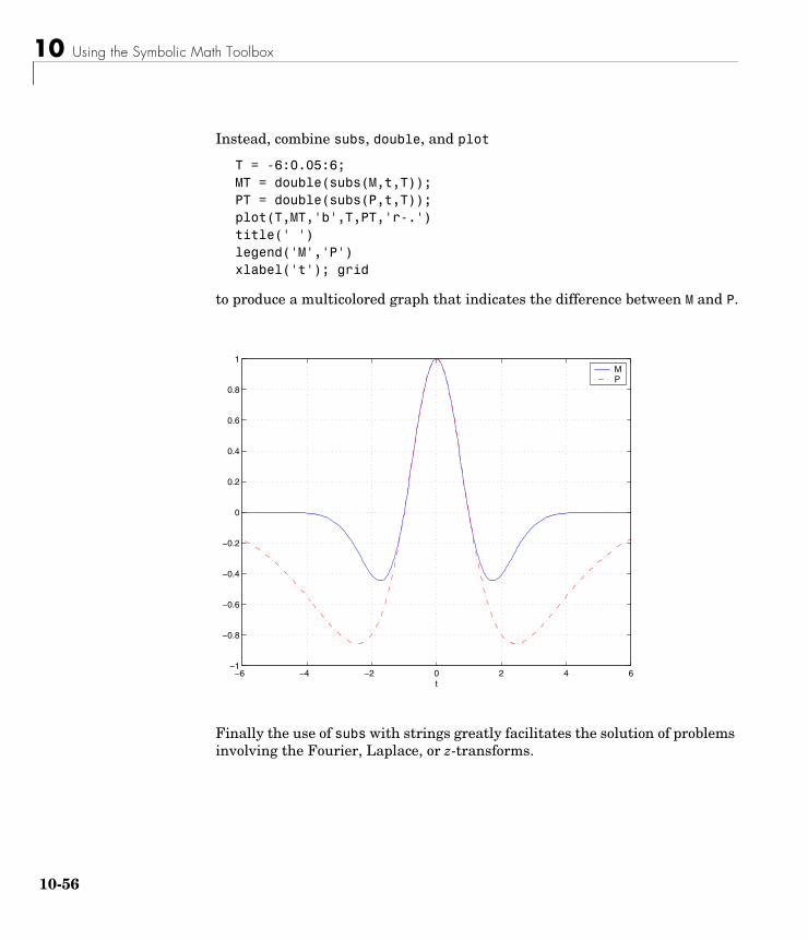
10 Using the Symbolic Math Toolbox
10-
Instead, combine subs, double, and plot
T = -6:0.05:6;MT = double(subs(M,t,T));PT = double(subs(P,t,T));plot(T,MT,'b',T,PT,'r-.')title(' ')legend('M','P')xlabel('t'); grid
to produce a multicolored graph that indicates the difference between M and P.
Finally the use of subs with strings greatly facilitates the solution of problems involving the Fourier, Laplace, or z-transforms.
−6 −4 −2 0 2 4 6−1
−0.8
−0.6
−0.4
−0.2
0
0.2
0.4
0.6
0.8
1
t
MP
56
Variable-Precision Arithmetic
Variable-Precision Arithmetic
OverviewThere are three different kinds of arithmetic operations in this toolbox:
For example, the MATLAB statements
format long1/2+1/3
use numeric computation to produce
0.83333333333333
With the Symbolic Math Toolbox, the statement
sym(1/2)+1/3
uses symbolic computation to yield
5/6
And, also with the toolbox, the statements
digits(25)vpa('1/2+1/3')
use variable-precision arithmetic to return
.8333333333333333333333333
The floating-point operations used by numeric arithmetic are the fastest of the three, and require the least computer memory, but the results are not exact. The number of digits in the printed output of MATLAB double quantities is controlled by the format statement, but the internal representation is always the eight-byte floating-point representation provided by the particular computer hardware.
Numeric MATLAB floating-point arithmetic
Rational Maple’s exact symbolic arithmetic
VPA Maple’s variable-precision arithmetic
10-57
10 Using the Symbolic Math Toolbox
10-
In the computation of the numeric result above, there are actually three roundoff errors, one in the division of 1 by 3, one in the addition of 1/2 to the result of the division, and one in the binary to decimal conversion for the printed output. On computers that use IEEE floating-point standard arithmetic, the resulting internal value is the binary expansion of 5/6, truncated to 53 bits. This is approximately 16 decimal digits. But, in this particular case, the printed output shows only 15 digits.
The symbolic operations used by rational arithmetic are potentially the most expensive of the three, in terms of both computer time and memory. The results are exact, as long as enough time and memory are available to complete the computations.
Variable-precision arithmetic falls in between the other two in terms of both cost and accuracy. A global parameter, set by the function digits, controls the number of significant decimal digits. Increasing the number of digits increases the accuracy, but also increases both the time and memory requirements. The default value of digits is 32, corresponding roughly to floating-point accuracy.
The Maple documentation uses the term “hardware floating-point” for what you are calling “numeric” or “floating-point” and uses the term “floating-point arithmetic” for what you are calling “variable-precision arithmetic.”
Example: Using the Different Kinds of Arithmetic
Rational ArithmeticBy default, the Symbolic Math Toolbox uses rational arithmetic operations, i.e., Maple’s exact symbolic arithmetic. Rational arithmetic is invoked when you create symbolic variables using the sym function.
The sym function converts a double matrix to its symbolic form. For example, if the double matrix is
A =1.1000 1.2000 1.30002.1000 2.2000 2.30003.1000 3.2000 3.3000
58
Variable-Precision Arithmetic
its symbolic form, S = sym(A), is
S =[11/10, 6/5, 13/10][21/10, 11/5, 23/10][31/10, 16/5, 33/10]
For this matrix A, it is possible to discover that the elements are the ratios of small integers, so the symbolic representation is formed from those integers. On the other hand, the statement
E = [exp(1) (1+sqrt(5))/2; log(3) rand]
returns a matrix
E = 2.71828182845905 1.61803398874989 1.09861228866811 0.76209683302739
whose elements are not the ratios of small integers, so sym(E) reproduces the floating-point representation in a symbolic form:
ans =[ 6121026514868074*2^(-51), 7286977268806824*2^(-52)][ 4947709893870346*2^(-52), 6864358026484820*2^(-53)]
Variable-Precision NumbersVariable-precision numbers are distinguished from the exact rational representation by the presence of a decimal point. A power of 10 scale factor, denoted by 'e', is allowed. To use variable-precision instead of rational arithmetic, create your variables using the vpa function.
For matrices with purely double entries, the vpa function generates the representation that is used with variable-precision arithmetic. For example, if you apply vpa to the matrix S defined in the preceding section, with digits(4), by entering
vpa(S)
10-59
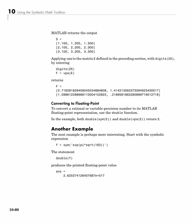
10 Using the Symbolic Math Toolbox
10-
MATLAB returns the output
S = [1.100, 1.200, 1.300][2.100, 2.200, 2.300][3.100, 3.200, 3.300]
Applying vpa to the matrix E defined in the preceding section, with digits(25), by entering
digits(25)F = vpa(E)
returns
F = [2.718281828459045534884808, 1.414213562373094923430017][1.098612288668110004152823, .2189591863280899719512718]
Converting to Floating-PointTo convert a rational or variable-precision number to its MATLAB floating-point representation, use the double function.
In the example, both double(sym(E)) and double(vpa(E)) return E.
Another ExampleThe next example is perhaps more interesting. Start with the symbolic expression
f = sym('exp(pi*sqrt(163))')
The statement
double(f)
produces the printed floating-point value
ans = 2.625374126407687e+017
60
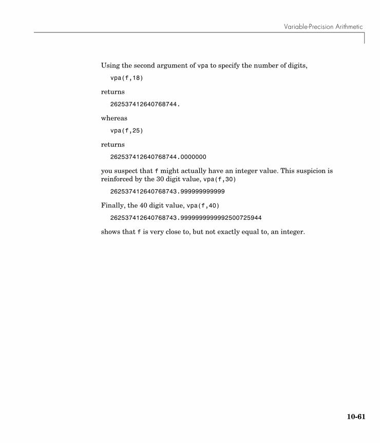
Variable-Precision Arithmetic
Using the second argument of vpa to specify the number of digits,
vpa(f,18)
returns
262537412640768744.
whereas
vpa(f,25)
returns
262537412640768744.0000000
you suspect that f might actually have an integer value. This suspicion is reinforced by the 30 digit value, vpa(f,30)
262537412640768743.999999999999
Finally, the 40 digit value, vpa(f,40)
262537412640768743.9999999999992500725944
shows that f is very close to, but not exactly equal to, an integer.
10-61
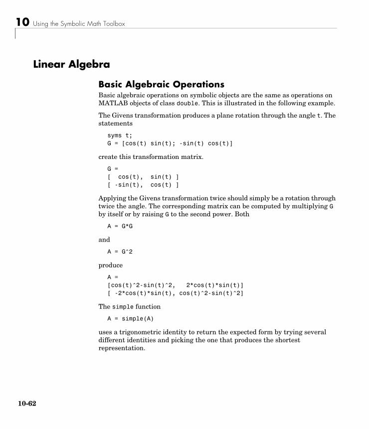
10 Using the Symbolic Math Toolbox
10-
Linear Algebra
Basic Algebraic OperationsBasic algebraic operations on symbolic objects are the same as operations on MATLAB objects of class double. This is illustrated in the following example.
The Givens transformation produces a plane rotation through the angle t. The statements
syms t;G = [cos(t) sin(t); -sin(t) cos(t)]
create this transformation matrix.
G =[ cos(t), sin(t) ][ -sin(t), cos(t) ]
Applying the Givens transformation twice should simply be a rotation through twice the angle. The corresponding matrix can be computed by multiplying G by itself or by raising G to the second power. Both
A = G*G
and
A = G^2
produce
A =[cos(t)^2-sin(t)^2, 2*cos(t)*sin(t)][ -2*cos(t)*sin(t), cos(t)^2-sin(t)^2]
The simple function
A = simple(A)
uses a trigonometric identity to return the expected form by trying several different identities and picking the one that produces the shortest representation.
62
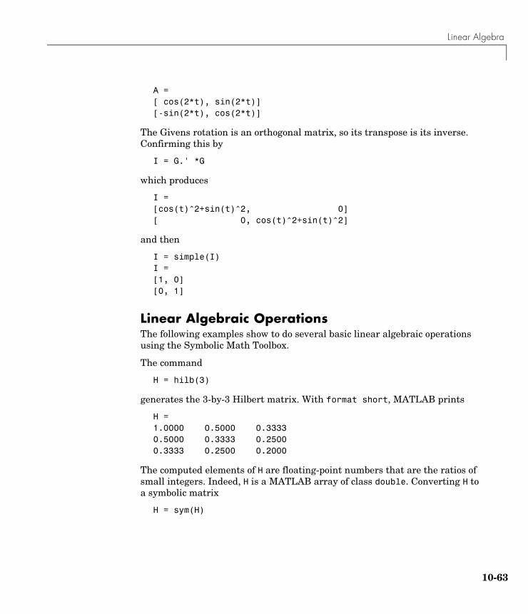
Linear Algebra
A =[ cos(2*t), sin(2*t)][-sin(2*t), cos(2*t)]
The Givens rotation is an orthogonal matrix, so its transpose is its inverse. Confirming this by
I = G.' *G
which produces
I =[cos(t)^2+sin(t)^2, 0][ 0, cos(t)^2+sin(t)^2]
and then
I = simple(I)I =[1, 0][0, 1]
Linear Algebraic OperationsThe following examples show to do several basic linear algebraic operations using the Symbolic Math Toolbox.
The command
H = hilb(3)
generates the 3-by-3 Hilbert matrix. With format short, MATLAB prints
H =1.0000 0.5000 0.33330.5000 0.3333 0.25000.3333 0.2500 0.2000
The computed elements of H are floating-point numbers that are the ratios of small integers. Indeed, H is a MATLAB array of class double. Converting H to a symbolic matrix
H = sym(H)
10-63
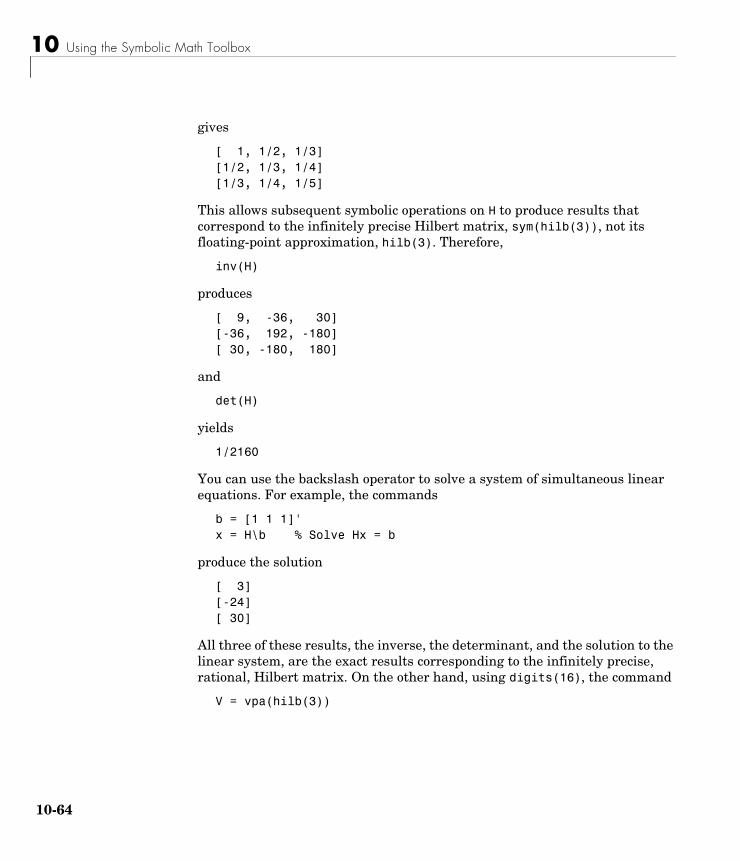
10 Using the Symbolic Math Toolbox
10-
gives
[ 1, 1/2, 1/3][1/2, 1/3, 1/4][1/3, 1/4, 1/5]
This allows subsequent symbolic operations on H to produce results that correspond to the infinitely precise Hilbert matrix, sym(hilb(3)), not its floating-point approximation, hilb(3). Therefore,
inv(H)
produces
[ 9, -36, 30][-36, 192, -180][ 30, -180, 180]
and
det(H)
yields
1/2160
You can use the backslash operator to solve a system of simultaneous linear equations. For example, the commands
b = [1 1 1]'x = H\b % Solve Hx = b
produce the solution
[ 3][-24][ 30]
All three of these results, the inverse, the determinant, and the solution to the linear system, are the exact results corresponding to the infinitely precise, rational, Hilbert matrix. On the other hand, using digits(16), the command
V = vpa(hilb(3))
64

Linear Algebra
returns
[ 1., .5000000000000000, .3333333333333333][.5000000000000000, .3333333333333333, .2500000000000000][.3333333333333333, .2500000000000000, .2000000000000000]
The decimal points in the representation of the individual elements are the signal to use variable-precision arithmetic. The result of each arithmetic operation is rounded to 16 significant decimal digits. When inverting the matrix, these errors are magnified by the matrix condition number, which for hilb(3) is about 500. Consequently,
inv(V)
which returns
ans =[ 9.000000000000179, -36.00000000000080, 30.00000000000067][ -36.00000000000080, 192.0000000000042, -180.0000000000040][ 30.00000000000067, -180.0000000000040, 180.0000000000038]
shows the loss of two digits. So does
det(V)
which gives
.462962962962953e-3
and
V\b
which is
[ 3.000000000000041][-24.00000000000021][ 30.00000000000019]
Since H is nonsingular, calculating the null space of H with the command
null(H)
returns an empty matrix, and calculating the column space of H with
colspace(H)
10-65
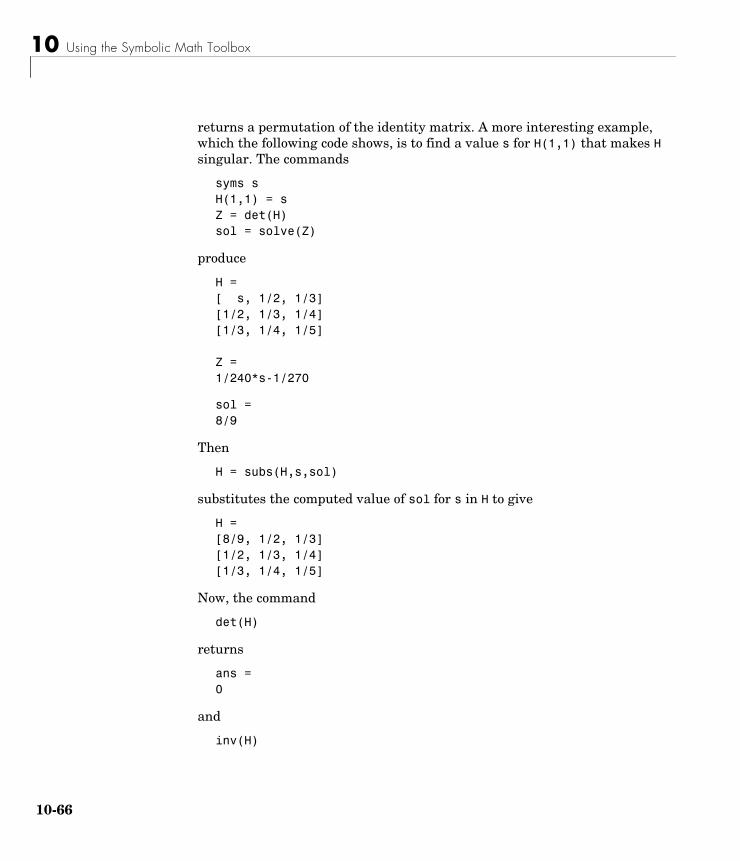
10 Using the Symbolic Math Toolbox
10-
returns a permutation of the identity matrix. A more interesting example, which the following code shows, is to find a value s for H(1,1) that makes H singular. The commands
syms sH(1,1) = sZ = det(H)sol = solve(Z)
produce
H =[ s, 1/2, 1/3][1/2, 1/3, 1/4][1/3, 1/4, 1/5]
Z =1/240*s-1/270
sol = 8/9
Then
H = subs(H,s,sol)
substitutes the computed value of sol for s in H to give
H =[8/9, 1/2, 1/3][1/2, 1/3, 1/4][1/3, 1/4, 1/5]
Now, the command
det(H)
returns
ans =0
and
inv(H)
66
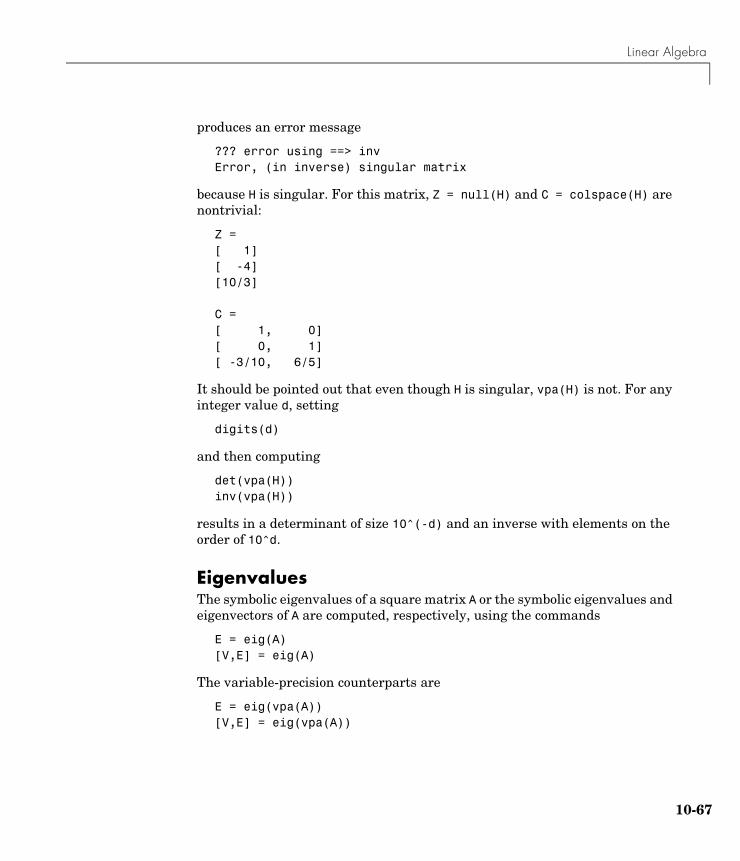
Linear Algebra
produces an error message
??? error using ==> invError, (in inverse) singular matrix
because H is singular. For this matrix, Z = null(H) and C = colspace(H) are nontrivial:
Z =[ 1][ -4][10/3]
C =[ 1, 0][ 0, 1][ -3/10, 6/5]
It should be pointed out that even though H is singular, vpa(H) is not. For any integer value d, setting
digits(d)
and then computing
det(vpa(H))inv(vpa(H))
results in a determinant of size 10^(-d) and an inverse with elements on the order of 10^d.
EigenvaluesThe symbolic eigenvalues of a square matrix A or the symbolic eigenvalues and eigenvectors of A are computed, respectively, using the commands
E = eig(A)[V,E] = eig(A)
The variable-precision counterparts are
E = eig(vpa(A))[V,E] = eig(vpa(A))
10-67
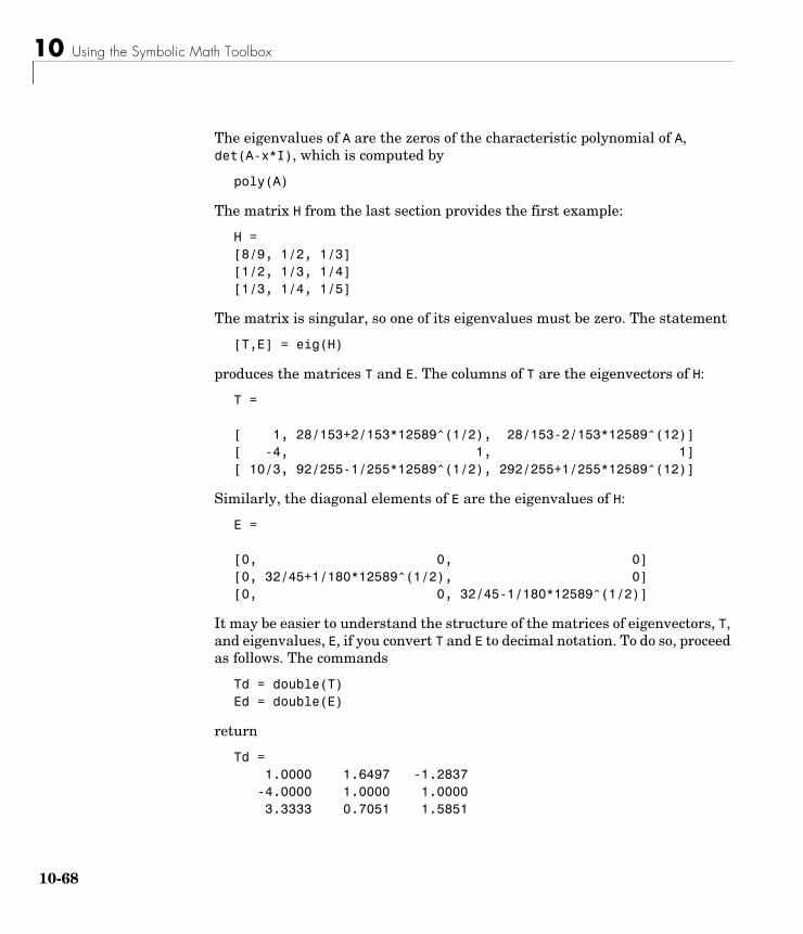
10 Using the Symbolic Math Toolbox
10-
The eigenvalues of A are the zeros of the characteristic polynomial of A, det(A-x*I), which is computed by
poly(A)
The matrix H from the last section provides the first example:
H =[8/9, 1/2, 1/3][1/2, 1/3, 1/4][1/3, 1/4, 1/5]
The matrix is singular, so one of its eigenvalues must be zero. The statement
[T,E] = eig(H)
produces the matrices T and E. The columns of T are the eigenvectors of H:
T = [ 1, 28/153+2/153*12589^(1/2), 28/153-2/153*12589^(12)][ -4, 1, 1][ 10/3, 92/255-1/255*12589^(1/2), 292/255+1/255*12589^(12)]
Similarly, the diagonal elements of E are the eigenvalues of H:
E = [0, 0, 0][0, 32/45+1/180*12589^(1/2), 0][0, 0, 32/45-1/180*12589^(1/2)]
It may be easier to understand the structure of the matrices of eigenvectors, T, and eigenvalues, E, if you convert T and E to decimal notation. To do so, proceed as follows. The commands
Td = double(T)Ed = double(E)
return
Td = 1.0000 1.6497 -1.2837 -4.0000 1.0000 1.0000 3.3333 0.7051 1.5851
68
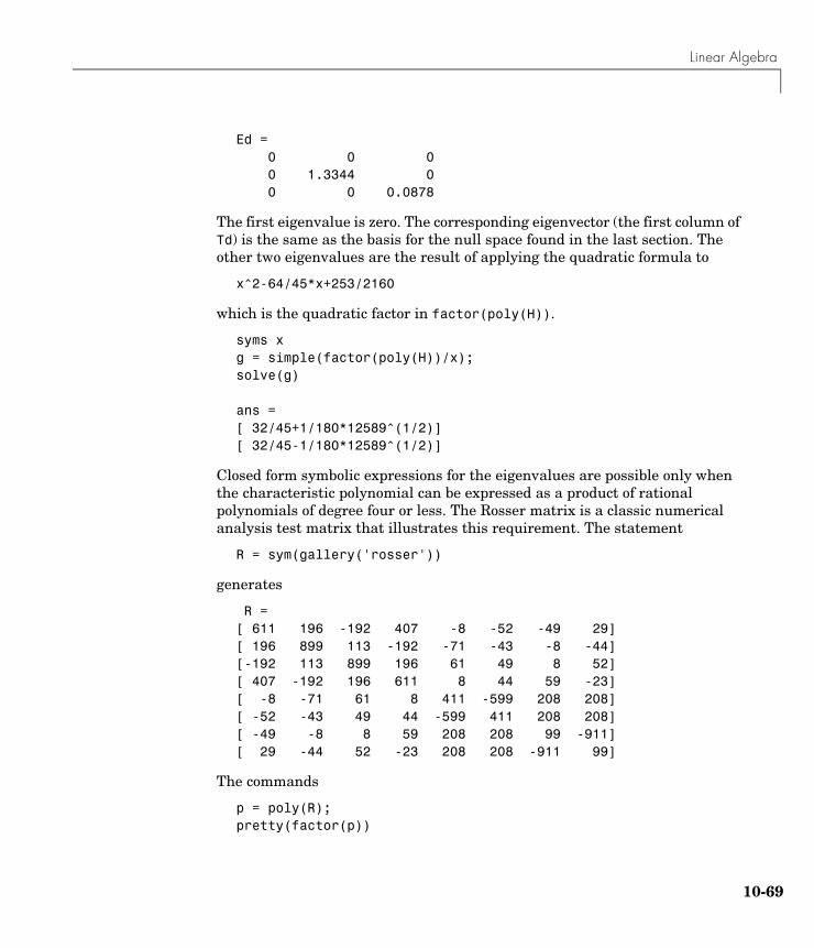
Linear Algebra
Ed = 0 0 0 0 1.3344 0 0 0 0.0878
The first eigenvalue is zero. The corresponding eigenvector (the first column of Td) is the same as the basis for the null space found in the last section. The other two eigenvalues are the result of applying the quadratic formula to
x^2-64/45*x+253/2160
which is the quadratic factor in factor(poly(H)).
syms xg = simple(factor(poly(H))/x);solve(g)
ans =[ 32/45+1/180*12589^(1/2)][ 32/45-1/180*12589^(1/2)]
Closed form symbolic expressions for the eigenvalues are possible only when the characteristic polynomial can be expressed as a product of rational polynomials of degree four or less. The Rosser matrix is a classic numerical analysis test matrix that illustrates this requirement. The statement
R = sym(gallery('rosser'))
generates
R = [ 611 196 -192 407 -8 -52 -49 29][ 196 899 113 -192 -71 -43 -8 -44][-192 113 899 196 61 49 8 52][ 407 -192 196 611 8 44 59 -23][ -8 -71 61 8 411 -599 208 208][ -52 -43 49 44 -599 411 208 208][ -49 -8 8 59 208 208 99 -911][ 29 -44 52 -23 208 208 -911 99]
The commands
p = poly(R);pretty(factor(p))
10-69
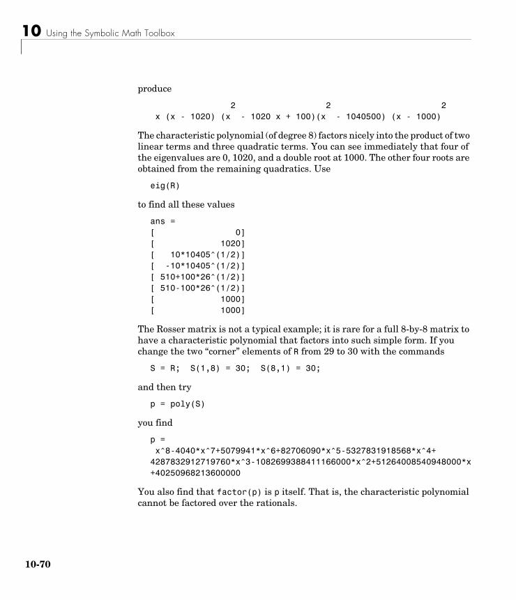
10 Using the Symbolic Math Toolbox
10-
produce
2 2 2 x (x - 1020) (x - 1020 x + 100)(x - 1040500) (x - 1000)
The characteristic polynomial (of degree 8) factors nicely into the product of two linear terms and three quadratic terms. You can see immediately that four of the eigenvalues are 0, 1020, and a double root at 1000. The other four roots are obtained from the remaining quadratics. Use
eig(R)
to find all these values
ans =[ 0][ 1020][ 10*10405^(1/2)][ -10*10405^(1/2)][ 510+100*26^(1/2)][ 510-100*26^(1/2)][ 1000][ 1000]
The Rosser matrix is not a typical example; it is rare for a full 8-by-8 matrix to have a characteristic polynomial that factors into such simple form. If you change the two “corner” elements of R from 29 to 30 with the commands
S = R; S(1,8) = 30; S(8,1) = 30;
and then try
p = poly(S)
you find
p = x^8-4040*x^7+5079941*x^6+82706090*x^5-5327831918568*x^4+4287832912719760*x^3-1082699388411166000*x^2+51264008540948000*x+40250968213600000
You also find that factor(p) is p itself. That is, the characteristic polynomial cannot be factored over the rationals.
70
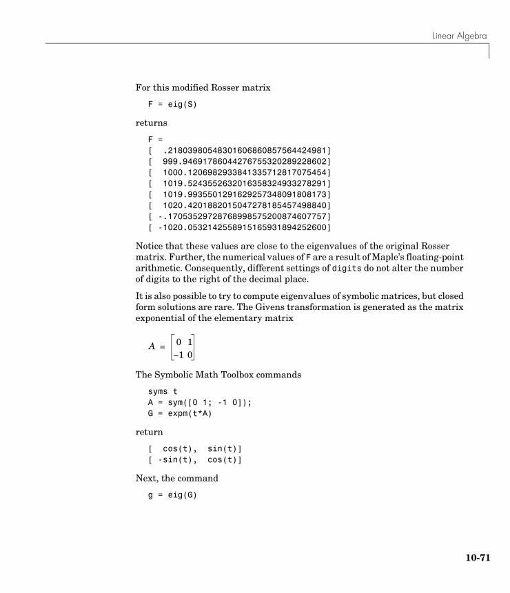
Linear Algebra
For this modified Rosser matrix
F = eig(S)
returns
F =[ .21803980548301606860857564424981][ 999.94691786044276755320289228602][ 1000.1206982933841335712817075454][ 1019.5243552632016358324933278291][ 1019.9935501291629257348091808173][ 1020.4201882015047278185457498840][ -.17053529728768998575200874607757][ -1020.0532142558915165931894252600]
Notice that these values are close to the eigenvalues of the original Rosser matrix. Further, the numerical values of F are a result of Maple’s floating-point arithmetic. Consequently, different settings of digits do not alter the number of digits to the right of the decimal place.
It is also possible to try to compute eigenvalues of symbolic matrices, but closed form solutions are rare. The Givens transformation is generated as the matrix exponential of the elementary matrix
The Symbolic Math Toolbox commands
syms tA = sym([0 1; -1 0]);G = expm(t*A)
return
[ cos(t), sin(t)][ -sin(t), cos(t)]
Next, the command
g = eig(G)
A 0 11– 0
=
10-71
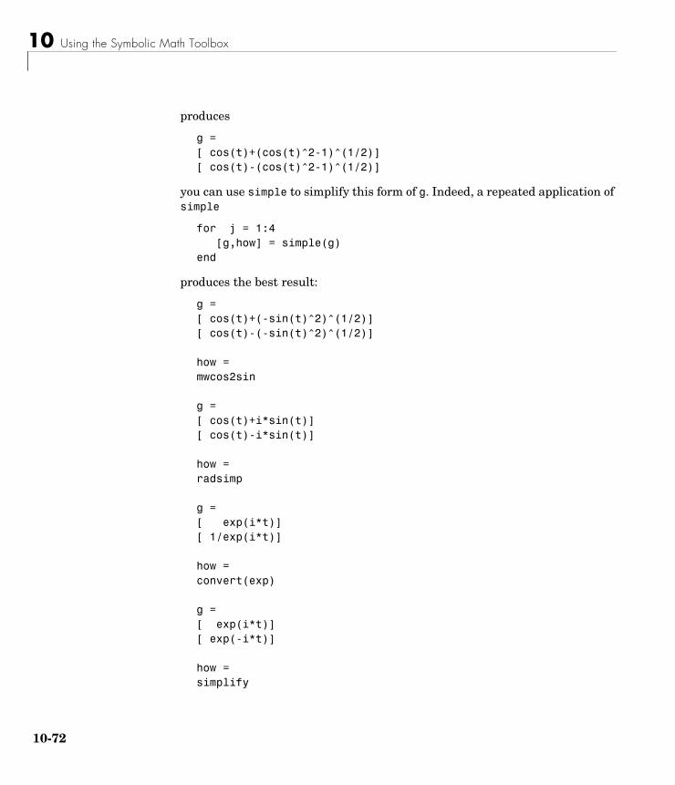
10 Using the Symbolic Math Toolbox
10-
produces
g =[ cos(t)+(cos(t)^2-1)^(1/2)][ cos(t)-(cos(t)^2-1)^(1/2)]
you can use simple to simplify this form of g. Indeed, a repeated application of simple
for j = 1:4[g,how] = simple(g)
end
produces the best result:
g =[ cos(t)+(-sin(t)^2)^(1/2)][ cos(t)-(-sin(t)^2)^(1/2)]
how =mwcos2sin
g =[ cos(t)+i*sin(t)][ cos(t)-i*sin(t)] how =radsimp g =[ exp(i*t)][ 1/exp(i*t)]
how =convert(exp)
g =[ exp(i*t)][ exp(-i*t)] how =simplify
72
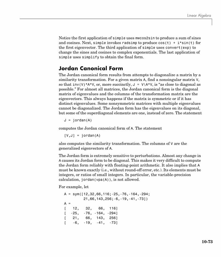
Linear Algebra
Notice the first application of simple uses mwcos2sin to produce a sum of sines and cosines. Next, simple invokes radsimp to produce cos(t) + i*sin(t) for the first eigenvector. The third application of simple uses convert(exp) to change the sines and cosines to complex exponentials. The last application of simple uses simplify to obtain the final form.
Jordan Canonical FormThe Jordan canonical form results from attempts to diagonalize a matrix by a similarity transformation. For a given matrix A, find a nonsingular matrix V, so that inv(V)*A*V, or, more succinctly, J = V\A*V, is “as close to diagonal as possible.” For almost all matrices, the Jordan canonical form is the diagonal matrix of eigenvalues and the columns of the transformation matrix are the eigenvectors. This always happens if the matrix is symmetric or if it has distinct eigenvalues. Some nonsymmetric matrices with multiple eigenvalues cannot be diagonalized. The Jordan form has the eigenvalues on its diagonal, but some of the superdiagonal elements are one, instead of zero. The statement
J = jordan(A)
computes the Jordan canonical form of A. The statement
[V,J] = jordan(A)
also computes the similarity transformation. The columns of V are the generalized eigenvectors of A.
The Jordan form is extremely sensitive to perturbations. Almost any change in A causes its Jordan form to be diagonal. This makes it very difficult to compute the Jordan form reliably with floating-point arithmetic. It also implies that A must be known exactly (i.e., without round-off error, etc.). Its elements must be integers, or ratios of small integers. In particular, the variable-precision calculation, jordan(vpa(A)), is not allowed.
For example, let
A = sym([12,32,66,116;-25,-76,-164,-294;21,66,143,256;-6,-19,-41,-73])
A =[ 12, 32, 66, 116][ -25, -76, -164, -294][ 21, 66, 143, 256][ -6, -19, -41, -73]
10-73
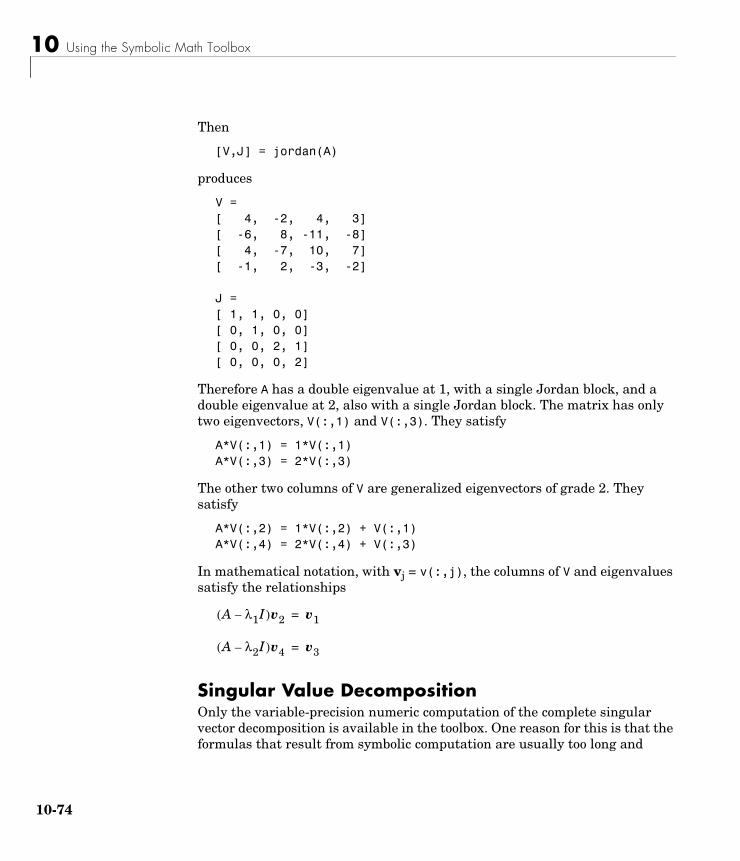
10 Using the Symbolic Math Toolbox
10-
Then
[V,J] = jordan(A)
produces
V =[ 4, -2, 4, 3][ -6, 8, -11, -8][ 4, -7, 10, 7][ -1, 2, -3, -2]
J =[ 1, 1, 0, 0][ 0, 1, 0, 0][ 0, 0, 2, 1][ 0, 0, 0, 2]
Therefore A has a double eigenvalue at 1, with a single Jordan block, and a double eigenvalue at 2, also with a single Jordan block. The matrix has only two eigenvectors, V(:,1) and V(:,3). They satisfy
A*V(:,1) = 1*V(:,1)A*V(:,3) = 2*V(:,3)
The other two columns of V are generalized eigenvectors of grade 2. They satisfy
A*V(:,2) = 1*V(:,2) + V(:,1)A*V(:,4) = 2*V(:,4) + V(:,3)
In mathematical notation, with vj = v(:,j), the columns of V and eigenvalues satisfy the relationships
Singular Value DecompositionOnly the variable-precision numeric computation of the complete singular vector decomposition is available in the toolbox. One reason for this is that the formulas that result from symbolic computation are usually too long and
A λ1I–( )v2 v1=
A λ2I–( )v4 v3=
74
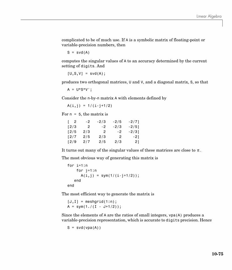
Linear Algebra
complicated to be of much use. If A is a symbolic matrix of floating-point or variable-precision numbers, then
S = svd(A)
computes the singular values of A to an accuracy determined by the current setting of digits. And
[U,S,V] = svd(A);
produces two orthogonal matrices, U and V, and a diagonal matrix, S, so that
A = U*S*V';
Consider the n-by-n matrix A with elements defined by
A(i,j) = 1/(i-j+1/2)
For n = 5, the matrix is
[ 2 -2 -2/3 -2/5 -2/7][2/3 2 -2 -2/3 -2/5][2/5 2/3 2 -2 -2/3][2/7 2/5 2/3 2 -2][2/9 2/7 2/5 2/3 2]
It turns out many of the singular values of these matrices are close to .
The most obvious way of generating this matrix is
for i=1:n for j=1:n A(i,j) = sym(1/(i-j+1/2));
endend
The most efficient way to generate the matrix is
[J,I] = meshgrid(1:n);A = sym(1./(I - J+1/2));
Since the elements of A are the ratios of small integers, vpa(A) produces a variable-precision representation, which is accurate to digits precision. Hence
S = svd(vpa(A))
π
10-75
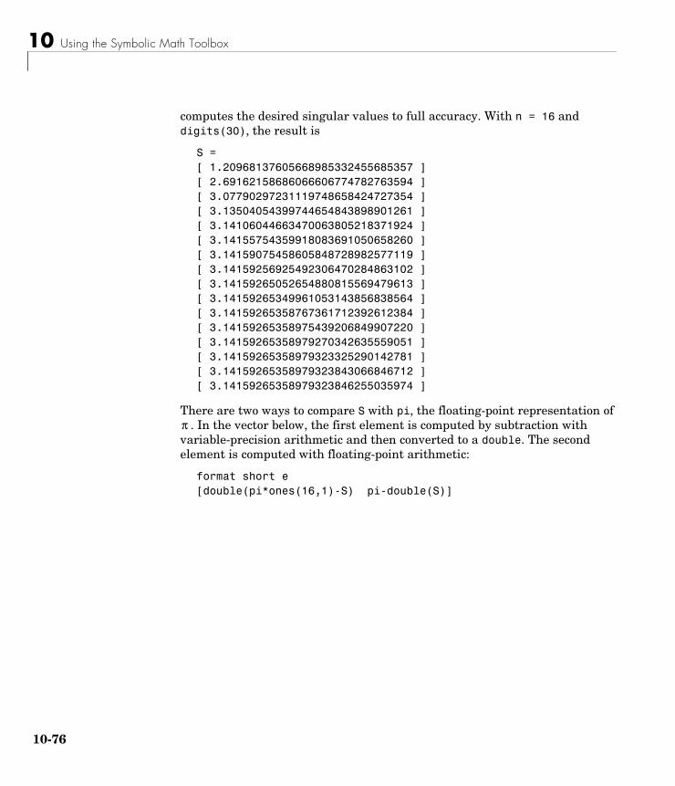
10 Using the Symbolic Math Toolbox
10-
computes the desired singular values to full accuracy. With n = 16 and digits(30), the result is
S = [ 1.20968137605668985332455685357 ][ 2.69162158686066606774782763594 ][ 3.07790297231119748658424727354 ][ 3.13504054399744654843898901261 ][ 3.14106044663470063805218371924 ][ 3.14155754359918083691050658260 ][ 3.14159075458605848728982577119 ][ 3.14159256925492306470284863102 ][ 3.14159265052654880815569479613 ][ 3.14159265349961053143856838564 ][ 3.14159265358767361712392612384 ][ 3.14159265358975439206849907220 ][ 3.14159265358979270342635559051 ][ 3.14159265358979323325290142781 ][ 3.14159265358979323843066846712 ][ 3.14159265358979323846255035974 ]
There are two ways to compare S with pi, the floating-point representation of . In the vector below, the first element is computed by subtraction with
variable-precision arithmetic and then converted to a double. The second element is computed with floating-point arithmetic:
format short e[double(pi*ones(16,1)-S) pi-double(S)]
π
76
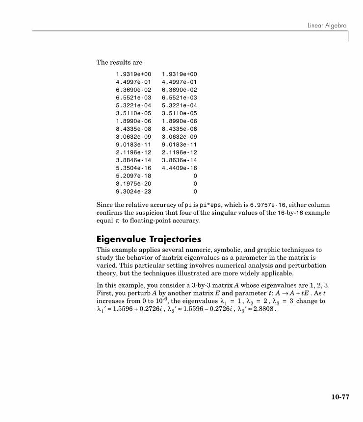
Linear Algebra
The results are
1.9319e+00 1.9319e+00 4.4997e-01 4.4997e-01 6.3690e-02 6.3690e-02 6.5521e-03 6.5521e-03 5.3221e-04 5.3221e-04 3.5110e-05 3.5110e-05 1.8990e-06 1.8990e-06 8.4335e-08 8.4335e-08 3.0632e-09 3.0632e-09 9.0183e-11 9.0183e-11 2.1196e-12 2.1196e-12 3.8846e-14 3.8636e-14 5.3504e-16 4.4409e-16 5.2097e-18 0 3.1975e-20 0 9.3024e-23 0
Since the relative accuracy of pi is pi*eps, which is 6.9757e-16, either column confirms the suspicion that four of the singular values of the 16-by-16 example equal to floating-point accuracy.
Eigenvalue TrajectoriesThis example applies several numeric, symbolic, and graphic techniques to study the behavior of matrix eigenvalues as a parameter in the matrix is varied. This particular setting involves numerical analysis and perturbation theory, but the techniques illustrated are more widely applicable.
In this example, you consider a 3-by-3 matrix A whose eigenvalues are 1, 2, 3. First, you perturb A by another matrix E and parameter . As t increases from 0 to 10-6, the eigenvalues , , change to
, , .
π
t: A A tE+→λ1 1= λ2 2= λ3 3=
λ1′ 1.5596 0.2726i+≈ λ2′ 1.5596 0.2726i–≈ λ3′ 2.8808≈
10-77
10 Using the Symbolic Math Toolbox
10-
This, in turn, means that for some value of , the perturbed matrix has a double eigenvalue . The example shows how to find the value of t, called , where this happens.
The starting point is a MATLAB test example, known as gallery(3).
A = gallery(3)A = -149 -50 -154 537 180 546 -27 -9 -25
This is an example of a matrix whose eigenvalues are sensitive to the effects of roundoff errors introduced during their computation. The actual computed eigenvalues may vary from one machine to another, but on a typical workstation, the statements
0 0.5 1 1.5 2 2.5 3 3.5
−0.3
−0.2
−0.1
0
0.1
0.2
0.3
λ(1) λ(2) λ(3)
λ’(1)
λ’(2)
λ’(3)
t τ 0 τ 10 6–< <,=A t( ) A tE+= λ1 λ2=
τ
78
Linear Algebra
format longe = eig(A)
produce
e = 1.00000000001122 1.99999999999162 2.99999999999700
Of course, the example was created so that its eigenvalues are actually 1, 2, and 3. Note that three or four digits have been lost to roundoff. This can be easily verified with the toolbox. The statements
B = sym(A);e = eig(B)'p = poly(B)f = factor(p)
produce
e =[1, 2, 3]
p =x^3-6*x^2+11*x-6
f =(x-1)*(x-2)*(x-3)
Are the eigenvalues sensitive to the perturbations caused by roundoff error because they are “close together”? Ordinarily, the values 1, 2, and 3 would be regarded as “well separated.” But, in this case, the separation should be viewed on the scale of the original matrix. If A were replaced by A/1000, the eigenvalues, which would be .001, .002, .003, would “seem” to be closer together.
But eigenvalue sensitivity is more subtle than just “closeness.” With a carefully chosen perturbation of the matrix, it is possible to make two of its eigenvalues coalesce into an actual double root that is extremely sensitive to roundoff and other errors.
10-79
10 Using the Symbolic Math Toolbox
10-
One good perturbation direction can be obtained from the outer product of the left and right eigenvectors associated with the most sensitive eigenvalue. The following statement creates
E = [130,-390,0;43,-129,0;133,-399,0]
the perturbation matrix
E =130 -390 0 43 -129 0133 -399 0
The perturbation can now be expressed in terms of a single, scalar parameter t. The statements
syms x tA = A+t*E
replace A with the symbolic representation of its perturbation:
A = [-149+130*t, -50-390*t, -154][ 537+43*t, 180-129*t, 546][ -27+133*t, -9-399*t, -25]
Computing the characteristic polynomial of this new A
p = poly(A)
gives
p =x^3-6*x^2+11*x-t*x^2+492512*t*x-6-1221271*t
Prettyprinting
pretty(collect(p,x))
shows more clearly that p is a cubic in x whose coefficients vary linearly with t.
3 2 x + (- t - 6) x + (492512 t + 11) x - 6 - 1221271 t
80
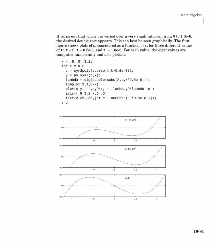
Linear Algebra
It turns out that when t is varied over a very small interval, from 0 to 1.0e-6, the desired double root appears. This can best be seen graphically. The first figure shows plots of p, considered as a function of x, for three different values of t: t = 0, t = 0.5e-6, and t = 1.0e-6. For each value, the eigenvalues are computed numerically and also plotted:
x = .8:.01:3.2; for k = 0:2c = sym2poly(subs(p,t,k*0.5e-6));y = polyval(c,x);lambda = eig(double(subs(A,t,k*0.5e-6)));subplot(3,1,3-k) plot(x,y,'-',x,0*x,':',lambda,0*lambda,'o')axis([.8 3.2 -.5 .5])text(2.25,.35,['t = ' num2str( k*0.5e-6 )]);
end
1 1.5 2 2.5 3−0.5
0
0.5t = 0
1 1.5 2 2.5 3−0.5
0
0.5t = 5e−007
1 1.5 2 2.5 3−0.5
0
0.5t = 1e−006
10-81
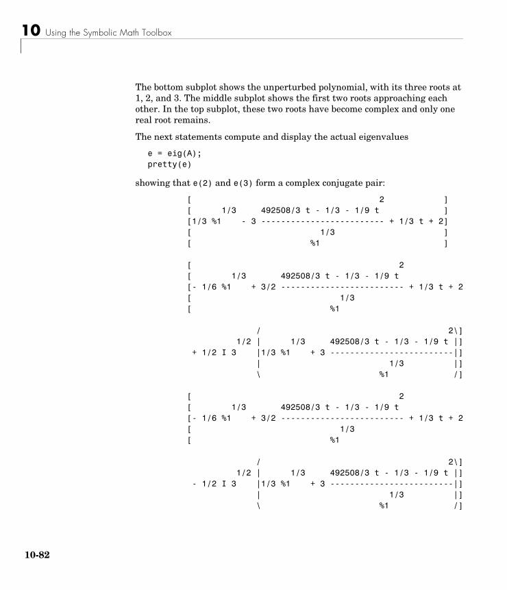
10 Using the Symbolic Math Toolbox
10-
The bottom subplot shows the unperturbed polynomial, with its three roots at 1, 2, and 3. The middle subplot shows the first two roots approaching each other. In the top subplot, these two roots have become complex and only one real root remains.
The next statements compute and display the actual eigenvalues
e = eig(A);pretty(e)
showing that e(2) and e(3) form a complex conjugate pair:
[ 2 ] [ 1/3 492508/3 t - 1/3 - 1/9 t ] [1/3 %1 - 3 ------------------------- + 1/3 t + 2] [ 1/3 ] [ %1 ]
[ 2 [ 1/3 492508/3 t - 1/3 - 1/9 t [- 1/6 %1 + 3/2 ------------------------- + 1/3 t + 2 [ 1/3 [ %1
/ 2\] 1/2 | 1/3 492508/3 t - 1/3 - 1/9 t |] + 1/2 I 3 |1/3 %1 + 3 -------------------------|] | 1/3 |] \ %1 /]
[ 2 [ 1/3 492508/3 t - 1/3 - 1/9 t [- 1/6 %1 + 3/2 ------------------------- + 1/3 t + 2 [ 1/3 [ %1
/ 2\] 1/2 | 1/3 492508/3 t - 1/3 - 1/9 t |] - 1/2 I 3 |1/3 %1 + 3 -------------------------|] | 1/3 |] \ %1 /]
82
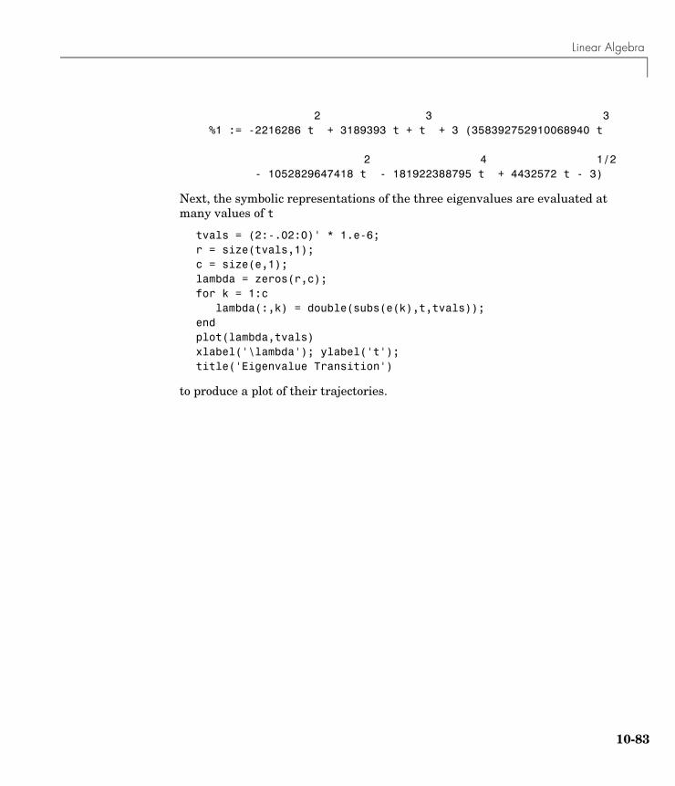
Linear Algebra
2 3 3 %1 := -2216286 t + 3189393 t + t + 3 (358392752910068940 t
2 4 1/2 - 1052829647418 t - 181922388795 t + 4432572 t - 3)
Next, the symbolic representations of the three eigenvalues are evaluated at many values of t
tvals = (2:-.02:0)' * 1.e-6;r = size(tvals,1);c = size(e,1);lambda = zeros(r,c);for k = 1:c
lambda(:,k) = double(subs(e(k),t,tvals));endplot(lambda,tvals)xlabel('\lambda'); ylabel('t');title('Eigenvalue Transition')
to produce a plot of their trajectories.
10-83
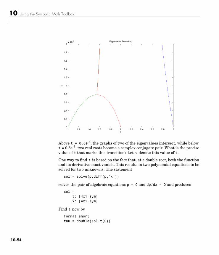
10 Using the Symbolic Math Toolbox
10-
Above t = 0.8e-6, the graphs of two of the eigenvalues intersect, while below t = 0.8e-6, two real roots become a complex conjugate pair. What is the precise value of t that marks this transition? Let denote this value of t.
One way to find is based on the fact that, at a double root, both the function and its derivative must vanish. This results in two polynomial equations to be solved for two unknowns. The statement
sol = solve(p,diff(p,'x'))
solves the pair of algebraic equations p = 0 and dp/dx = 0 and produces
sol = t: [4x1 sym] x: [4x1 sym]
Find now by
format shorttau = double(sol.t(2))
1 1.2 1.4 1.6 1.8 2 2.2 2.4 2.6 2.8 30
0.2
0.4
0.6
0.8
1
1.2
1.4
1.6
1.8
2x 10
−6
λ
t
Eigenvalue Transition
τ
τ
τ
84
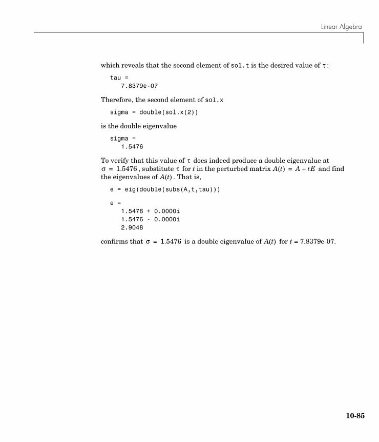
Linear Algebra
which reveals that the second element of sol.t is the desired value of :
tau =7.8379e-07
Therefore, the second element of sol.x
sigma = double(sol.x(2))
is the double eigenvalue
sigma =1.5476
To verify that this value of does indeed produce a double eigenvalue at , substitute for t in the perturbed matrix and find
the eigenvalues of . That is,
e = eig(double(subs(A,t,tau)))
e = 1.5476 + 0.0000i 1.5476 - 0.0000i 2.9048
confirms that is a double eigenvalue of for t = 7.8379e-07.
τ
τσ 1.5476= τ A t( ) A tE+=
A t( )
σ 1.5476= A t( )
10-85
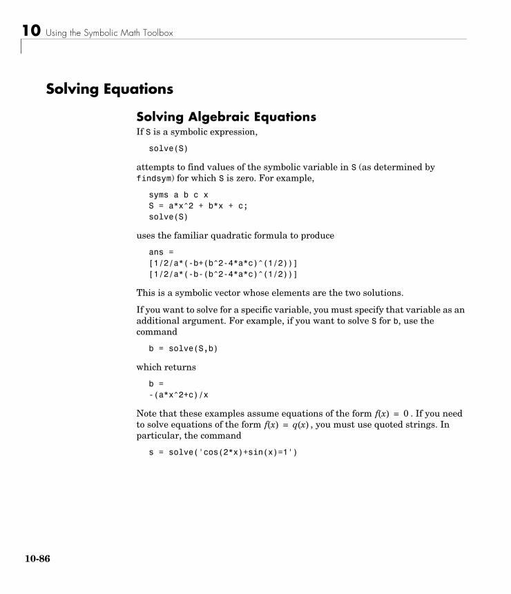
10 Using the Symbolic Math Toolbox
10-
Solving Equations
Solving Algebraic EquationsIf S is a symbolic expression,
solve(S)
attempts to find values of the symbolic variable in S (as determined by findsym) for which S is zero. For example,
syms a b c xS = a*x^2 + b*x + c;solve(S)
uses the familiar quadratic formula to produce
ans =[1/2/a*(-b+(b^2-4*a*c)^(1/2))][1/2/a*(-b-(b^2-4*a*c)^(1/2))]
This is a symbolic vector whose elements are the two solutions.
If you want to solve for a specific variable, you must specify that variable as an additional argument. For example, if you want to solve S for b, use the command
b = solve(S,b)
which returns
b =-(a*x^2+c)/x
Note that these examples assume equations of the form . If you need to solve equations of the form , you must use quoted strings. In particular, the command
s = solve('cos(2*x)+sin(x)=1')
f x( ) 0=f x( ) q x( )=
86
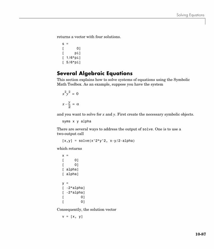
Solving Equations
returns a vector with four solutions.
s =[ 0][ pi][ 1/6*pi][ 5/6*pi]
Several Algebraic EquationsThis section explains how to solve systems of equations using the Symbolic Math Toolbox. As an example, suppose you have the system
and you want to solve for x and y. First create the necessary symbolic objects.
syms x y alpha
There are several ways to address the output of solve. One is to use a two-output call
[x,y] = solve(x^2*y^2, x-y/2-alpha)
which returns
x = [ 0][ 0][ alpha][ alpha]
y = [ -2*alpha][ -2*alpha][ 0][ 0]
Consequently, the solution vector
v = [x, y]
x2y2 0=
x y2---– α=
10-87
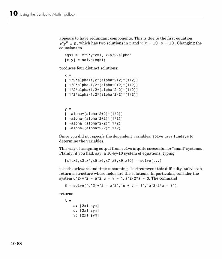
10 Using the Symbolic Math Toolbox
10-
appears to have redundant components. This is due to the first equation , which has two solutions in x and y: , . Changing the
equations to
eqs1 = 'x^2*y^2=1, x-y/2-alpha'[x,y] = solve(eqs1)
produces four distinct solutions:
x =[ 1/2*alpha+1/2*(alpha^2+2)^(1/2)][ 1/2*alpha-1/2*(alpha^2+2)^(1/2)][ 1/2*alpha+1/2*(alpha^2-2)^(1/2)][ 1/2*alpha-1/2*(alpha^2-2)^(1/2)] y =[ -alpha+(alpha^2+2)^(1/2)][ -alpha-(alpha^2+2)^(1/2)][ -alpha+(alpha^2-2)^(1/2)][ -alpha-(alpha^2-2)^(1/2)]
Since you did not specify the dependent variables, solve uses findsym to determine the variables.
This way of assigning output from solve is quite successful for “small” systems. Plainly, if you had, say, a 10-by-10 system of equations, typing
[x1,x2,x3,x4,x5,x6,x7,x8,x9,x10] = solve(...)
is both awkward and time consuming. To circumvent this difficulty, solve can return a structure whose fields are the solutions. In particular, consider the system u^2-v^2 = a^2, u + v = 1, a^2-2*a = 3. The command
S = solve('u^2-v^2 = a^2','u + v = 1','a^2-2*a = 3')
returns
S = a: [2x1 sym] u: [2x1 sym] v: [2x1 sym]
x2y2 0= x 0±= y 0±=
88
Solving Equations
The solutions for a reside in the “a-field” of S. That is,
S.a
produces
ans =[ 3][ -1]
Similar comments apply to the solutions for u and v. The structure S can now be manipulated by field and index to access a particular portion of the solution. For example, if you want to examine the second solution, you can use the following statement
s2 = [S.a(2), S.u(2), S.v(2)]
to extract the second component of each field.
s2 =[ -1, 1, 0]
The following statement
M = [S.a, S.u, S.v]
creates the solution matrix M
M = [ 3, 5, -4][ -1, 1, 0]
whose rows comprise the distinct solutions of the system.
Linear systems of simultaneous equations can also be solved using matrix division. For example,
clear u v x ysyms u v x yS = solve(x+2*y-u, 4*x+5*y-v);sol = [S.x;S.y]
10-89
10 Using the Symbolic Math Toolbox
10-
and
A = [1 2; 4 5];b = [u; v];z = A\b
result in
sol = [ -5/3*u+2/3*v][ 4/3*u-1/3*v]
z =[ -5/3*u+2/3*v][ 4/3*u-1/3*v]
Thus s and z produce the same solution, although the results are assigned to different variables.
Single Differential EquationThe function dsolve computes symbolic solutions to ordinary differential equations. The equations are specified by symbolic expressions containing the letter D to denote differentiation. The symbols D2, D3, ... DN, correspond to the second, third, ..., Nth derivative, respectively. Thus, D2y is the Symbolic Math Toolbox equivalent of . The dependent variables are those preceded by D and the default independent variable is t. Note that names of symbolic variables should not contain D. The independent variable can be changed from t to some other symbolic variable by including that variable as the last input argument.
Initial conditions can be specified by additional equations. If initial conditions are not specified, the solutions contain constants of integration, C1, C2, etc.
The output from dsolve parallels the output from solve. That is, you can call dsolve with the number of output variables equal to the number of dependent variables or place the output in a structure whose fields contain the solutions of the differential equations.
d2y dt2⁄
90
Solving Equations
Example 1The following call to dsolve
dsolve('Dy=1+y^2')
uses y as the dependent variable and t as the default independent variable.
The output of this command is
ans = tan(t+C1)
To specify an initial condition, use
y = dsolve('Dy=1+y^2','y(0)=1')
This produces
y =tan(t+1/4*pi)
Notice that y is in the MATLAB workspace, but the independent variable t is not. Thus, the command diff(y,t) returns an error. To place t in the workspace, type syms t.
Example 2Nonlinear equations may have multiple solutions, even when initial conditions are given:
x = dsolve('(Dx)^2+x^2=1','x(0)=0')
results in
x =[ sin(t)][ -sin(t)]
Example 3Here is a second order differential equation with two initial conditions. The commands
y = dsolve('D2y=cos(2*x)-y','y(0)=1','Dy(0)=0', 'x');simplify(y)
10-91
10 Using the Symbolic Math Toolbox
10-
produce
ans =4/3*cos(x)-2/3*cos(x)^2+1/3
The key issues in this example are the order of the equation and the initial conditions. To solve the ordinary differential equation
simply type
u = dsolve('D3u=u','u(0)=1','Du(0)=-1','D2u(0) = pi','x')
Use D3u to represent and D2u(0) for .
Several Differential EquationsThe function dsolve can also handle several ordinary differential equations in several variables, with or without initial conditions. For example, here is a pair of linear, first-order equations.
S = dsolve('Df = 3*f+4*g', 'Dg = -4*f+3*g')
The computed solutions are returned in the structure S. You can determine the values of f and g by typing
f = S.ff = exp(3*t)*(C1*sin(4*t)+C2*cos(4*t))
g = S.gg =exp(3*t)*(C1*cos(4*t)-C2*sin(4*t))
If you prefer to recover f and g directly as well as include initial conditions, type
[f,g] = dsolve('Df=3*f+4*g, Dg =-4*f+3*g', 'f(0) = 0, g(0) = 1')
x3
3
d
d u u=
u 0( ) 1 u′ 0( ), 1, u″ 0( )– π= = =
d3u dx3⁄ u′′ 0( )
92
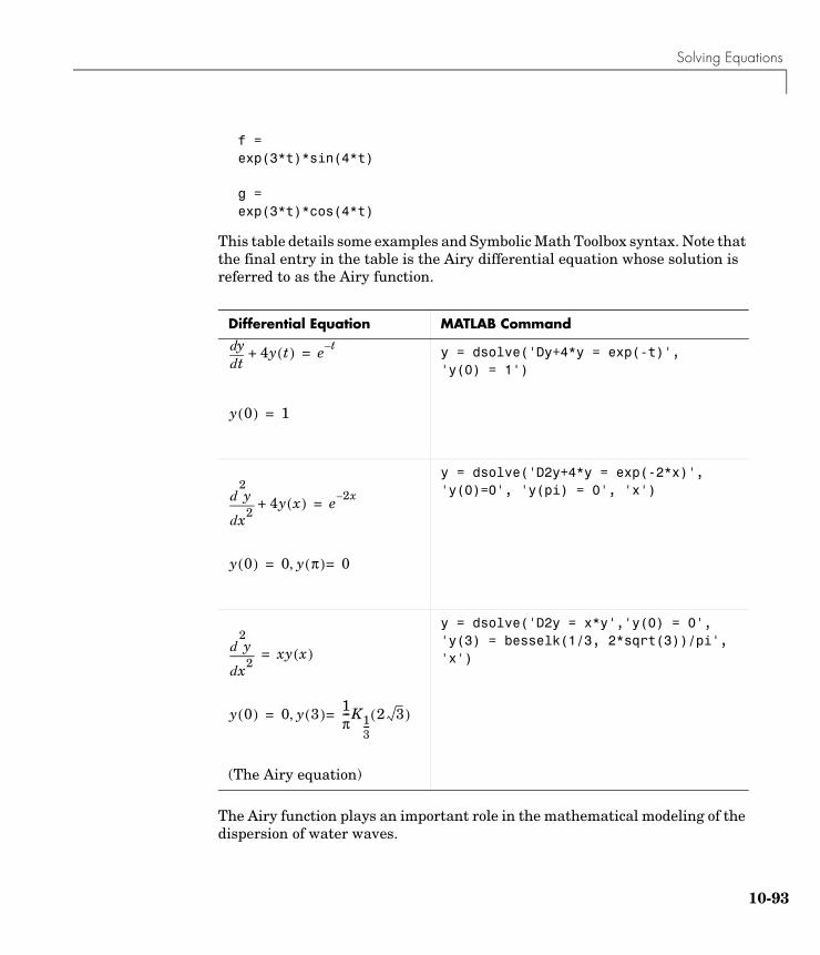
Solving Equations
f =exp(3*t)*sin(4*t)
g =exp(3*t)*cos(4*t)
This table details some examples and Symbolic Math Toolbox syntax. Note that the final entry in the table is the Airy differential equation whose solution is referred to as the Airy function.
The Airy function plays an important role in the mathematical modeling of the dispersion of water waves.
Differential Equation MATLAB Command
y = dsolve('Dy+4*y = exp(-t)', 'y(0) = 1')
y = dsolve('D2y+4*y = exp(-2*x)', 'y(0)=0', 'y(pi) = 0', 'x')
(The Airy equation)
y = dsolve('D2y = x*y','y(0) = 0', 'y(3) = besselk(1/3, 2*sqrt(3))/pi', 'x')
tddy 4y t( )+ e t–
=
y 0( ) 1=
x2
2
d
d y 4y x( )+ e 2x–=
y 0( ) 0 y π( ) 0=,=
x2
2
d
d y xy x( )=
y 0( ) 0 y 3( ) 1π---K1
3---
2 3( )=,=
10-93

10 Using the Symbolic Math Toolbox
10-
94
Index
Symbols: operator 4-7@sym directory 9-15\ 10-64
Aabstract functions 9-13activating Student Version
on Linux 2-17on Mac OS X 2-8on Windows 2-3
activation 1-4administrator status on OS X 2-8Airy differential equation 10-93Airy function 10-93algorithms
vectorizing 6-31animation 5-71annotating plots 5-16ans function 4-4application program interface (API) 3-3Array Editor 8-12array operators 4-22arrays
cell 6-11character 6-13columnwise organization 4-24creating in M-files 4-15deleting rows and columns 4-17elements 4-11generating with functions and operators 4-14listing contents 4-10loading from external data files 4-15and matrices 4-21multidimensional 6-9notation for elements 4-11
preallocating 6-31structure 6-16variable names 4-10
arrow keys for editing commands 4-30aspect ratio of axes 5-48AVI files 5-71axes
managing 5-48visibility 5-49
axis 5-49axis function 5-48
Bbackslash operator 10-64Bessel functions
differentiating 10-5integrating 10-13
besselj 10-5besselk 10-93bit map 5-59blockset 3-4books
MATLAB related 1-9break function 6-7built-in functions
defined 4-12
Ccalculus 10-2
example 10-20extended example 10-28
callbacks 7-6case function 6-4catch function 6-8
Index-1
Index
Ind
cell arrays 6-11char function 6-15character arrays 6-13characteristic polynomial 4-21circulant matrix 9-13clear 9-12clearing variables 9-12collect 10-42colon operator 4-7colormap 5-54colors
lines for plotting 5-41column space 10-65Command History 8-5command line
editing 4-30Command Window 8-4comp.soft-sys.matlab 1-10complex numbers
plotting 5-43complex symbolic variables 9-12concatenation 4-16
strings 6-14configuring additional products
on Windows 2-5conj 9-12constants
special 4-12continue function 6-6continuing statements on multiple lines 4-30control keys for editing commands 4-30converting symbolic matrices to numeric form
9-11current directory 8-9Current Directory browser 8-9
ex-2
Ddata source 5-27debugging M-files 8-13decimal symbolic expressions 9-10default symbolic variable 9-9definite integration 10-12deleting array elements 4-17demos
MATLAB 1-6running from the Start button 8-3
desktop for MATLAB 3-7desktop tools 8-1determinant of matrix 4-19diag function 4-4diff 10-2differentiation 10-2digits 9-11documentation 8-6
Mac OS X 2-15double
converting to floating-point with 10-60dsolve 10-90
Eediting command lines 4-30Editor/Debugger 8-13eig 10-67eigenvalue 4-20eigenvalue trajectories 10-77eigenvalues 10-67
computing 10-67eigenvector 4-20elements of arrays 4-11entering matrices 4-3eps 9-10erase mode 5-71
Index
eval function 6-27executing MATLAB 3-7exiting MATLAB 3-7expand 10-43exporting graphs 5-35expressions
evaluating 6-27examples 4-13using in MATLAB 4-10
Ffactor
example 10-44factorial function 9-13figure function 5-46figure tools 5-7figure windows 5-46
with multiple plots 5-46find function 4-27finding object handles 5-69fliplr function 4-6floating-point arithmetic 10-57
IEEE 10-58floating-point numbers 4-11floating-point symbolic expressions 9-10flow control 6-2for loop 6-5format
of output display 4-28format 10-57format function 4-28function functions 6-28function handles
defined 6-28using 6-30
function keyword 6-22
function M-files 6-19naming 6-21
function of two variables 5-52functions
built-in, defined 4-12defined 6-21finding specific 1-7how to find 4-12running 8-4variable number of arguments 6-22
GGivens transformation 10-62global variables 6-25golden ratio 9-5graphical user interface
creating 7-1laying out 7-3programming 7-6
graphicsfiles 5-60Handle Graphics 5-62objects 5-63printing 5-60
grids 5-49GUIDE 7-1
HHandle Graphics 5-62
defined 3-3finding handles 5-69
Helpaccessing on Linux 2-22accessing on Mac OS X 2-14accessing on Windows 2-14
Index-3
Index
Ind
helpsources of 1-9via newsgroup 1-10
Help browser 8-6help functions 8-8Hilbert matrix 9-11hold function 5-44horner
example 10-43
IIEEE floating-point arithmetic 10-58if function 6-2images 5-58imaginary numbers 4-11installation root directory
specifying on Linux 2-19installing Student Version
on Linux 2-17on Mac OS X 2-8on Windows 2-3
installing toolboxeson Linux 2-22on Mac OS X 2-14on Windows 2-5
int 10-11integration 10-11
definite 10-12with real constants 10-13
Jjacobian 10-6Jacobian matrix 10-6jordan
example 10-73
ex-4
Jordan canonical form 10-73
Kkeys for editing in Command Window 4-30
Llearning MATLAB 1-6legend
adding to plot 5-40legend function 5-40library
mathematical function 3-3lighting 5-55limit 10-8limits 10-8
axes 5-48undefined 10-10
line continuation 4-30line styles of plots 5-41linear algebra 10-62Linux
activating Student Version 2-17installing Student Version 2-17
load function 4-15loading arrays 4-15local variables 6-22log of functions used 8-5logical vectors 4-26
MMac OS X
activating Student Version 2-8documentation 2-15installing Student Version 2-8

Index
machine epsilon 9-10Maclaurin series 10-19magic function 4-8magic square 4-4Maple 9-2Maple functions
accessing 9-13markers 5-41MAT-file 5-58mathematical function library 3-3mathematical functions
listing advanced 4-12listing elementary 4-12listing matrix 4-12
MathWorks Storepurchasing products from 1-9
MathWorks Web site 1-9MATLAB
application program interface 3-3books 1-9calling C subroutine on Linux 2-16calling C subroutine on Mac OS X 2-7calling C subroutine on Windows 2-2calling Fortran subroutine on Linux 2-16calling Fortran subroutine on Mac OS X 2-7calling Fortran subroutine on Windows 2-2demos 1-6desktop 3-7executing 3-7exiting 3-7history 3-2how to learn 1-6language 3-3mathematical function library 3-3overview 3-2quitting 3-7running 3-7
shutting down 3-7starting 3-7starting on Linux 2-22
MATLAB Central 1-10matlab command
setting up symbolic link on Linux 2-21MATLAB user newsgroup 8-8matrices 4-18
creating 4-14entering 4-3
matrix 4-2antidiagonal 4-6condition number 10-65determinant 4-19main diagonal 4-5multiplication 4-18singular 4-19swapping columns 4-8symmetric 4-18transpose 4-4
mesh plot 5-52mex command
setting up symbolic link on Linux 2-21MEX-file
Linux 2-16Mac OS X 2-7supported Windows compilers 2-3Windows 2-2
M-filesand toolboxes 3-3creating 6-19editing 8-13for creating arrays 4-15function 6-19script 6-19
Microsoft Word and access to MATLAB 8-18M-Lint Code Checker 8-15
Index-5
Index
Ind
movies 5-73multidimensional arrays 6-9multiple data sets
plotting 5-40multiple plots per figure 5-46multivariate data
organizing 4-24
Nnewsgroup 1-10newsgroup for MATLAB users 8-8Notebook 8-18null space 10-65numbers 4-11
floating-point 4-11numeric symbolic expressions 9-10
Oobject properties 5-65objects
finding handles 5-69graphics 5-63
online helpviewing 8-6
operators 4-11colon 4-7
outputcontrolling format 4-28suppressing 4-30
overlaying plots 5-44
Ppath 8-10plot function 5-38
ex-6
plotsediting 5-16
plottingadding legend 5-40adding plots 5-44basic 5-38complex data 5-43complex numbers 5-43contours 5-44editing 5-16functions 5-38line colors 5-41line styles 5-41lines and markers 5-41mesh and surface 5-52multiple data sets 5-40multiple plots 5-46overview 5-2tools 5-9
poly 10-68PostScript 5-61preallocation 6-31presentation graphics 5-29pretty
example 10-19print function 5-60Printing 5-33printing
example 5-33graphics 5-60
professional versiondifferences with Student Version 1-11
Profiler 8-17Property Editor
interface 5-19Property Inspector 5-18
Index
Qquitting MATLAB 3-7
Rrational arithmetic 10-58rational symbolic expressions 9-10real property 9-12real symbolic variables 9-12reference information
obtaining 1-7return function 6-8revision control systems
interfacing to MATLAB 8-18root directory
specifying on Linux 2-19Rosser matrix 10-69running functions 8-4running MATLAB 3-7
Sscalar expansion 4-25scientific notation 4-11screens
installation data 2-21root directory on Linux 2-19
scripts 6-20search path 8-10semicolon to suppress output 4-30shutting down MATLAB 3-7simple 10-46simplifications 10-41simplify 10-46Simulink 3-4simultaneous differential equations
solving 10-92
simultaneous linear equationssolving systems of 10-64
singular matrix 4-19singular value decomposition 10-74solve 10-86solving equations 10-86
algebraic 10-86ordinary differential 10-90
source control systemsinterfacing to MATLAB 8-18
special constantsinfinity 4-13not-a-number 4-13
specialized graphs 5-45spherical coordinates 10-6Start button 8-3starting MATLAB 3-7startup.m file
Windows 2-4Stateflow 3-4statements
continuing on multiple lines 4-30executing 6-27
statusadministrator on OS X 2-8
stringsconcatenating 6-14
structures 6-16Student Version
differences with professional version 1-11installing on Linux 2-17installing on Mac OS X 2-8installing on Windows 2-3MATLAB differences 1-11Simulink differences 1-11Symbolic Math Toolbox differences 1-12
subexpr 10-50
Index-7
Index
Ind
subexpressions 10-50subplot function 5-46subs 10-52subscripting
with logical vectors 4-26subscripts 4-6substitutions 10-50sum function 4-4summation
symbolic 10-18support
sources of 1-9suppressing output 4-30surface plot 5-52svd 10-75switch function 6-4sym 9-5symbolic expressions 10-86
creating 9-5decimal 9-10floating-point 9-10numeric 9-10rational 9-10
symbolic linkssetting up 2-21
symbolic math functionscreating 9-15
Symbolic Math Toolboxlearning 1-7
symbolic matrixcomputing eigenvalue of 10-70converting to numeric form 9-11creating 9-13differentiating 10-5
symbolic objectsabout 9-3
symbolic summation 10-18
ex-8
symbolic variablescomplex 9-12creating 9-5real 9-12
symmetric matrix 4-18syms 9-6symsum 10-18system requirements
Linux 2-16Mac OS X 2-7Windows 2-2
Ttaylor 10-18Taylor series 10-18technical support 1-10text
entering in MATLAB 6-13TIFF 5-61title
figure 5-49toolboxes 3-2
installing on Linux 2-22installing on Mac OS X 2-14installing on Windows 2-5
tools in the desktop 8-1transpose function 4-4troubleshooting 1-8try function 6-8
Vvariable-precision arithmetic 10-57variable-precision numbers 10-59variables 4-10
global 6-25
Index
local 6-22vectorization 6-31vectors 4-2
logical 4-26preallocating 6-31
version control systemsinterfacing to MATLAB 8-18
visibility of axes 5-49vpa 10-59
Wwhile loop 6-6Windows
activating Student Version 2-3installing Student Version 2-3
windows for plotting 5-46windows in MATLAB 3-7wireframe
surface 5-52Word and access to MATLAB 8-18word processing access to MATLAB 8-18workspace 8-11Workspace browser 8-11www.mathworks.com 1-9www.mathworks.com/academia 1-9www.mathworks.com/store 1-9www.mathworks.com/support/books 1-9
Xxor erase mode 5-71
Index-9

Index
Ind
ex-10