Optimal Vacation Itinerary Modeling

MATH 381: OPTIMAL VACATION ROUTING

GERARD TRIMBERGER, YIZHOU YAO, SIMENG ZHU, AND JOHN CHAFFEE

Abstract. This project aims to find optimal vacation options for a trav-

eler. A complete graph is constructed with vertexes representing cities and

edges representing the distance between two adjacent cities. Two problemsare solved: the classic traveling salesperson problem, as well as a maximal

traveling salesperson problem in which the route is adjusted to maximize total

cost. In addition, related problems that included ratings for individual citieswere posed and solved. The results are finally discussed in terms of cost and

travel distance.

Contents

1. Introduction 22. Background 23. Model 33.1. Traveling Salesperson Problem 33.2. Best Trip 43.3. Implementation Challenges 54. Solution 64.1. Sage Solution 64.2. Matlab MTZ Solution 64.3. Visualization 65. Discussion 76. Model Variations 86.1. TSP Maximum Mileage 86.2. TSP Happiness Factors/Mileage Requirements 107. Conclusions 12References 12A. Problem Data 12B. Visualization 14

1

2 GERARD TRIMBERGER, YIZHOU YAO, SIMENG ZHU, AND JOHN CHAFFEE

1. Introduction

We started with the concept of world travel with the goal of visiting 20 pre-determined cities. More specifically, we were interested in finding optimal routesthat would take the traveler through each city exactly once. In order to get con-crete routing results, we first constructed a fully connected graph whose vertexeswere the cities and whose edges represented the distance[5] between adjacent cities.We later updated the data to include factors for each city such as GDP[2], costof living[4], number of museums[6], and number of malls[1]. These problems areclosely related to the well-known traveling salesperson problem, which is solvablewith linear programming.

In addition to using linear programming to find optimal solutions, we also madeuse of multidimensional scaling in order to visualize our results.

2. Background

In our first meeting, we brainstormed a list of general topics that we were inter-ested in so that each member felt connected to the project. John suggested that wefocus on something related to graphs or graph theory, specifically the TSP. Gerardwas interested in a problem similar to the Netflix algorithm, where a library of userratings generate a network of suggested movies. Simeng mentioned that he wasinterested in currency conversion, which led to the idea of creating an internationalproblem.

We were eventually drawn to TSP-related problems because of the rich and far-reaching theory behind them. TSP problems were first defined in the 1800s byW.R. Hamilton, although serious study and progress on the problem did not takeoff until the 1930s. Since then, traveling salesman type problems have becomeubiquitous and have driven advances in both the study of graph theory and, after1970, algorithms for solving linear programs. Using a TSP-type problem, we wereall enabled to explore our individual interests.

We chose 20 cities that we felt were globally recognized as travel destinationsand had a fairly diverse geographical distribution, (i.e. Seattle, Miami, New York,Stockholm, Reykjavik, Moscow, Saint Petersburg, New Delhi, Shanghai, Chengdu,Tokyo, Rio de Jeneiro, Cairo, Johannesburg, London, Sydney, Paris, Oslo, Hon-olulu, and Bangkok.) As for the costs of the edges between the travel vertices, weoriginally wanted to consider airfare and hotel pricing in each city. However, thevariance in realtime airfare and hotel pricing was hard to overlook, so we settled ongeographical distance as a more consistent, yet relevant, measure of cost betweentwo cities. An argument can be made that there is a correlation between geograph-ical distance and airfare pricing when considering the additional fuel required forlonger versus shorter flights.

Next, we generated a list of possible happiness factors that we could define foreach city. The list included: number of restaurants in the city, carbon footprint,whether or not the city has an amusement park, number of museums or libraries,number of art galleries, nightlife (number of clubs/bars), number of sporting are-nas/teams, average cost of living, GDP number of shopping malls, etc. We thenscoured the internet for quantititive attraction data for each of the above mentionedcities. In the end, we were able to find a cost of living index[4], restauarant index[4],purchasing power index[4], GDP[2], and number of shopping malls for each city.

MATH 381: OPTIMAL VACATION ROUTING 3

3. Model

Consider a graph G which is made up of a set of vertices V and a set of edges E.The entry vi represents the label for vertex i, while an element (i, j) of E indicatesthat vertex i is adjacent (connected) to vertex j. More specifically, let G be aweighted graph such that ci,j = cj,i is the weight of the edge connecting vertex ito vertex j if (i, j) ∈ E, and zero otherwise. Then we can construct an adjacencymatrix:

(1) A = (ci,j).

For our problem that is centered around travel between n = 20 cities, ci,j is the“cost” of travel between city i and city j – we chose this cost to be representedby the physical distance between them. Refer to Table 6 in Appendix A for thecorrespondence between city name and vertex.

Figure 1. Complete Graph with 20 Nodes

The graph G, and its corresponding adjacency matrix A, can be used to deter-mine several different types of optimal routing schemes.

3.1. Traveling Salesperson Problem. Suppose we wish to find the route of leastcost which passes through each city exactly once and ends up at the starting city.This problem is known as the Traveling Salesperson Problem, or TSP. The TSPcan be solved by the use of integer linear programming through the Miller-Tucker-Zemlin (MTZ) formulation[3]. The MTZ formulation relies on :


3.1.1. MTZ Formulation. Suppose we have n cities that we wish to visit on ouritinerary. We number the cities 1, . . . , n and define

(2) xi,j =

{1 if there exists an edge between city i and city j

0 otherwise

Define ci,j to be the ”cost,” or geographical distance, of traveling from city i tocity j. Introduce the dummy variables ui, where i = 1, . . . , n, which representsthe itinerary number for each of the locations, e.g. u1 represents when ’Seattle’ isvisited, which is always first (i.e. u1 = 1), and u2 represents when Miami is visited,which depends on the solution of the TSP. Therefore, the LP can be written as

Minimize:∑i,j

ci,jxi,j

Subject to:∑i

xi,j = 1 for j = 1, 2, . . . , n (1)∑j

xi,j = 1 for i = 1, 2, . . . , n (2)

u1 = 1, 2 ≤ ui ≤ n for i = 2, . . . , n (3)

ui − uj + 1 ≤ (n− 1)(1− xi,j) for i, j ≥ 2 (4)

0 ≤ xi,j ≤ 1 for all i, j (5)

xi,j ∈ Z (6)

(1) ensures that there is exactly one trip into and out of each city

(2) compliments (1)

(3) introduces a dummy variable for ensuring that the path found is Hamilton-ian

(4) ensures that the solution path is made of one loop

(5) limits xi,j to the domain [0, 1] and

(6) together with (5) ensures that xi,j is binary

3.2. Best Trip. As mentioned previously, our ultimate goal for creating the MTZformulation of the TSP was to utilize it as a springboard to more complex models.We then wanted to modify the TSP problem to find the best possible trip in termsof city sequence. Specifically, we agreed that the trip would be better if the goodcities were visited in sequence, when possible, with the added constraint that thetotal trip must cover a certain minimum distance. In order to do this, we gatheredquantitative data on several “factors of happiness” for each city on our map, andused that data to formulate a rating for each city.

3.2.1. City Rating Scheme. Consider the matrix F which contains the raw ratingdata for the n cities:

(3) F =[f1|f2| . . . |fm

].


Here, column m corresponds to the m-th city rating factor, and each column hasits own units and distribution. In order to standardize the factor matrix F , wesubtract from each column its own minimum value and then divide that differenceby the difference between the maximum and minimum values in that column. Thatis, if F ∗ represents the standardized factor matrix, then

(4) f∗m =fm −min(fm)

max(fm)−min(fm)

Next, consider a vector w = [w1, w2, . . . , wm]> which contains the relativeweights for each of the rating factors. The weighted city rating vector can thenbe written as

(5) r = F ∗w =[w1f

∗1 + w2f

∗2 + · · ·+ wmf∗m

]The total city rating for city i is then ri.

3.2.2. New LP Constraints. With this additional happiness factor in mind, a newlinear program can be written to determine the best route for a given budget.

Consider a scaled cost variable c∗i,j = kci,j−min(A)

max(A)−min(A) . Then, we can also add a

constraint that the total cost of the trip be above a certain level M . Keeping alloriginal constraints, new LP can be written as

Maximize:∑i,j

[(k − c∗i,j)(ri + rj)xi,j ]

Subject to:∑i,j

ci,jxi,j ≥M (1)

∑i

xi,j = 1 for j = 1, 2, . . . , n (2)∑j

xi,j = 1 for i = 1, 2, . . . , n (3)

u1 = 1, 2 ≤ ui ≤ n for i = 2, . . . , n (4)

ui − uj + 1 ≤ (n− 1)(1− xi,j) for i, j ≥ 2 (5)

0 ≤ xi,j ≤ 1 for all i, j (6)

xi,j ∈ Z (7)

This formulation is very similar to the traveling salesperson problem. The mainchanges are that the objective function is now set to maximize a weighted sum ofscaled ratings of the cities that our traveler passes through. The “cost” is now(k − c∗i,j)(ri + rj), which is large when ri and rj and both large and c∗i,j is small.This causes our LP to look for routes which group the best cities together – that is,it looks for Hamiltonian paths which minimize the distance between the best cities.

3.3. Implementation Challenges. One challenge that we encountered while im-plementing the TSP in Sage was the lack of versatility within the program whichprevented us from adding additional constraints to the standard TSP. Therefore,we decided to implement our problem by utilizing the Matlab function mxlpsolve

to generate an LPsolve script to solve the problem.


First, we attempted to solve the TSP for the 20 aforementioned cities but the in-efficiencies of the MTZ formulation led to extremely long calculation times. There-fore, we decided to reduce the number of vacation destination to the 13 locationswith the most city data: Seattle, Miami, New York, Shanghai, Chengdu, Tokyo,Rio de Janeiro, Cairo, Johannesburg, London, Sydney, Paris, and Bangkok. Thisallowed us to perform the optimization calculations in a much more reasonableperiod of time, while preserving the majority of the model’s complexity.

4. Solution

A folder containing all coded inputs and outputs is available at https://drive.google.com/drive/folders/0B0qQ-1OAi1JkRXZzMHJFMENPU0E?usp=sharing.

4.1. Sage Solution. Using Sage, we obtained the optimal solution to the TravelingSalesman Problem. The code for this problem was very straightforward, and onlytook a few lines to implement. We utlized the built in Sage commands for creatingGraphs and solving for their respective TSP solutions.

4.2. Matlab MTZ Solution. For the Matlab implementation of the MTZ, webegan by importing the distance matrix from a locally stored Excel document. Wethen used the length() command to calculate the number of cities in our data set,n. We created a binary n × n matrix X, where the xij entry represents whetheror not there is an edge between city i and city j. The distance data was used tocreate an n × n cost matrix C. A vector of dummy variables u was used to storethe itinerary number of each city. The mxlpsolve package for Matlab allows theuser to choose from a library of commands that ultimately write the LP to an .lp

file, which can then be opened, run, and solved in lpsolve1.We began by setting the variable names xij for i, j = 1, . . . , n and ui for i =

1, . . . , n. We then defined the objective function as a row vector f where the entriesfi are the corresponding coefficient for each variable in the objective function.For constraint (1), we utilize the ’set binary’ command, which ensures that thevariables xij ∈ {0, 1} for i, j = 1, . . . , n. For constraint (2), we used the commandadd constraint to restrict u1 = 1 and ui ∈ {2, . . . , n}, i = 2, . . . , n which ensuresthat each city falls into an available iternary spot, and that Seattle, location 1,is the starting and ending point. Constraints (3), (4), and (5) were added ina similar manner, utlizing the add constraint command and following the logicoutlined above. Finally, we called the write lp command to write a .lp file, whichcontainted all of the aforementioned logic, to be opened and executed in lpsolve toproduce a solution.

The solution to the TSP, results in a total mileage cost of 50,109 miles.

4.3. Visualization. Using multidimensional scaling, a projection onto two dimen-sional euclidean space can be made to visualize the distances between the cities.We used the MATLAB function mdscale to get this projection from the inter-citydistances found in Appendix A. The optimized routes were then drawn onto thisprojection. These figures can be found in in Appendix B.

1http://web.mit.edu/lpsolve/doc/MATLAB.htm

https://drive.google.com/drive/folders/0B0qQ-1OAi1JkRXZzMHJFMENPU0E?usp=sharing

https://drive.google.com/drive/folders/0B0qQ-1OAi1JkRXZzMHJFMENPU0E?usp=sharing

http://web.mit.edu/lpsolve/doc/MATLAB.htm


Table 1. MTZ solution of TSP for 13 cities

nonzero xi j variables Departure, city i Arrival, city jx1 12 Seattle Parisx12 10 Paris Londonx10 7 London Rio de Janeirox7 8 Rio de Janeiro Cairox8 9 Cairo Johannesburgx9 11 Johannesburg Sydneyx11 6 Sydney Tokyox6 5 Tokyo ChengDux5 4 ChengDu ShangHaix4 13 ShangHai Bangkokx13 3 Bangkok New Yorkx3 2 New York Miamix2 1 Miami Seattle

5. Discussion

From our result in last section about the least total mileage possible to travelthrough all our chosen cities at least once, we can go one step ahead and gaininteresting insight on the possible cost it would at least take for one to take suchtrip in real life.

Below is a graph on economy class airfares displayed by Rome2rio users overthe past 4 months, totaling some 1,780,832 price points. Airfares are grouped bydistance and selected the 20-th percentile fare for each distance (where 20% of faresare less and 80% are more), to produce the following graph:

We can see that it shows an almost linear relationship between the airfare andthe flight distance. In a simplified manner, we can estimate the relationship with alinear model:

Fare = $50 + (Distance ∗ $0.11/mile)


Where Fare is the cost in $USD of flying Distance miles. On average, a farecosts $50 before any flight distance is taken into account, plus an average of 11cents per mile traveled.

With this linear airfare model, the average amount a person will spend on a TSPitinerary through all 13 cities will be:

avg. TSP fare = $50 + (50109 ∗ $0.11) = $5561.99

It’s the cheapest average because our cost model here is based entirely on mileagetraveled, and our TSP model provides a path with minimal miles necessary.

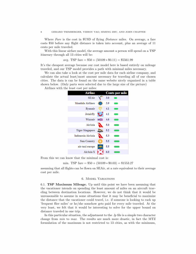
We can also take a look at the cost per mile data for each airline company, andcalculate the actual least/most amount necessary for traveling all of our chosencities. The data is can be found on the same website nicely organized in a tableshown below. (Only parts were selected due to the large size of the picture)

Airlines with the least cost per miles:

From this we can know that the minimal cost is:

min. TSP fare = $50 + (50109 ∗ $0.03) = $1553.27

assuming that all flights can be flown on SEAir, at a rate equivalent to their averagecost per mile.

6. Model Variations

6.1. TSP Maximum Mileage. Up until this point we have been assuming thatthe vacationer intends on spending the least amount of miles on an aircraft trav-eling between destination locations. However, we do not think that it would beunreasonable to assume in some situations that it may be beneficial to maximizethe distance that the vacationer could travel, i.e. if someone is looking to rack up’frequent flier miles’ or he/she somehow gets paid for every mile traveled. At thevery least, we felt that it would be interesting to solve for the upper bound ondistance traveled in one trip.

In this particular situation, the adjustment to the .lp file is a simple two characterchange from min to max. The results are much more drastic, in fact the MTZformulation of the maximum is not restricted to 13 cities, as with the minimum,


and can in fact be solved for the original set of 20 cities that we started with. Theresults of both are presented in the tables below.

Table 2. Most Costly MTZ solution of TSP for 20 cities

nonzero xi j variables Departure, city i Arrival, city jx1 14 Seattle Johannesburgx14 7 Johannesburg St. Petersburgx7 2 St. Petersburg Miamix2 6 Miami Moscowx6 3 Moscow New Yorkx3 8 New York New Dehlix8 5 New Dehli Reykjavikx5 20 Reykjavik Bangkokx20 18 Bangkok Oslox18 16 Oslo Sydneyx16 17 Sydney Parisx17 9 Paris ShangHaix9 12 ShangHai Rio de Janeirox12 11 Rio de Janeiro Tokyox11 15 Tokyo Londonx15 10 London ChengDux10 4 ChengDu Stockholmx4 19 Stockholm Honolulux19 13 Honolulu Cairox13 1 Cairo Seattle

Table 3. Most Costly MTZ solution of TSP for 13 cities

nonzero xi j variables Departure, city i Arrival, city jx1 9 Seattle Johannesburgx9 13 Johannesburg Bangkokx13 12 Bangkok Parisx12 11 Paris Sydneyx11 3 Sydney New Yorkx3 4 New York ShangHaix4 7 ShangHai Rio de Janeirox7 6 Rio de Janeiro Tokyox6 10 Tokyo Londonx10 5 London ChengDux5 2 ChengDu Miamix2 8 Miami Cairox8 1 Cairo Seattle


The results in table 2 and table 3 immediately makes sense because they includeas many far apart pairs of cities in the trip. Almost all flights cross continent.Many flights cross equator and go to the other half of the globe (i.e., from Oslo toSydney). It’s possibly not the usual way people would travel, as it often goes backand forth between continents, ignoring close-by destinations. However, for purposeof maximizing the total mileage, this is a solid solution. With 20 destinations, themaximum mileage possible is 142,601 and with 13 destinations, it is 105,361. Thisprovides an upper bound to TSP solutions for both cases. Now let’s reconsider thecost per mile model we discussed in section 5. Here we can calculate the interestingvalue of maximum cost a man can spend travelling all chosen cities.

avg. TSP fare20 = $50 + (142, 601 ∗ $0.11) = $15, 736.11

avg. TSP fare13 = $50 + (105, 361 ∗ $0.11) = $11, 639.71

Therefore, the resulting average cost for a maximum mileage TSP solution of the20 and 13 destinations cases, is $15,736.11 and $11,639.71 respectively. This isroughly three times the cost of traveling through the minimal cost route.

Taking it one step further, we can incorporate the airlines with the most costper miles, as shown below:

From this we can calculate the maximum cost of a 20 destination trip would be,

max TSP fare20 = 142, 601 ∗ $0.278 = $39, 643.08

and the cost of a 13 destination trip would be,

max TSP fare13 = 105, 361 ∗ $0.278 = $29, 290.36

assuming that all flights could be booked through Darwin Airlines at the averagefare of $0.278 per mile.

6.2. TSP Happiness Factors/Mileage Requirements. Another variation tothe TSP that we decided to investigate was changing the objective function of theTSP to include our happiness factors, discussed in section 3.2, and creating a newconstraint that involves a minimum mileage requirement. In essence, we are stillsolving the TSP for the least ”costly” solution, but we are altering the definition


cost. The happiness factors now influence the cost, and we are instead maximizinghappiness while meeting a specific mileage goal. The happiness rating for eachflight is inversely proportional to the length of the flight so the model still has aninherent ability to solve for the shortest path. This is where the mileage requirementcomes in. For example, if there is no mileage requirement then we are solving forthe TSP of the new, happiness factor based objective function, i.e. the trip withthe maximum happiness as defined in section 3.2. The corresponding solution ispresented below:

Table 4. Happiness factor TSP for 13 cities, no trip min.

nonzero xi j variables Departure, city i Arrival, city jx1 2 Seattle Miamix2 12 Miami Parisx12 10 Paris Londonx10 7 London Rio de Janeirox7 8 Rio de Janeiro Cairox8 9 Cairo Johannesburgx9 11 Johannesburg Sydneyx11 6 Sydney Tokyox6 5 Tokyo ChengDux5 4 ChengDu ShangHaix4 13 ShangHai Bangkokx13 3 Bangkok New Yorkx3 1 New York Seattle

By summing flight distance of each of the above-mentioned flights, we can solvefor the minimum travel distance, 52,414 miles, while maximizing happiness. How-ever, if we increase the mileage threshold above that of the solution of the TSP,then we start to see new solutions emerge. For example, if we set the minimummileage threshold to 55,000 miles, then the optimal solution changes.

Table 5. Happiness TSP for 13 cities, 55,000 mi. trip min.

nonzero xi j variables Departure, city i Arrival, city jx1 2 Seattle Miamix2 9 Miami Johannesburgx9 7 Johannesburg Rio de Janeirox7 5 Rio de Janeiro ChengDux5 8 ChengDu Cairox8 4 Cairo ShangHaix4 6 ShangHai Tokyox6 11 Tokyo Sydneyx11 13 Sydney Bangkokx13 12 Bangkok Parisx12 10 Paris Londonx10 3 London New Yorkx3 1 New York Seattle


7. Conclusions

In this project, we first solved the basic TSP model minimizng total mileage.Then we also solved a few variations of the original problem (maximizing mileage,maximizing happiness factor... etc.) For all problems, our model with a graphapproach yields results that not only satisfies all constraints but also looks realistic.In other words, the travel plans our model provides are close to what a reasonableplan maker might actually use in real life. On this account, I think our approachin using a graph model on the Traveling Salesperson Problem and its variations isa sensible one.

The results of the TSP problem and its variations provides interesting insightsinto the real-life travel plan making. For each different purpose, our model providesthe following advices/facts:

• The least amount of flight fare, on average, to travel through all 13 citiesat least once is $ 5561.99.• On average, the most that one will spend to visit each of the 13 destination

once will be $ 11,639.71.• However if we take into account the minimum distance at the cheapest

airfare, and the maximum distance at the most expensive prices, we canestimate a range of prices that all possible trips through these locationsshould fall within, $ 1,553.27 to $ 29,290.36. This range may seem quitewide for the typical traveller, but from a mathematician’s perspective thesenumbers intuitively seems to be on the correct order of magnititude forstandard international travel.

References

[1] Google maps maps.google.com.

[2] A. Berube, J. L. Trujillo, T. Ran, and J. Parilla. Report: Global metro monitor. BrookingsInstitute.

[3] C. E. Miller, A. W. Tucker, and R. A. Zemlin. Integer programming formulation of traveling

salesman problems. J. ACM, 7(4):326–329, October 1960.[4] Numbeo. Cost of living: https://www.numbeo.com/cost-of-living/.

[5] Geobytes Distance Tool: http://geobytes.com/citydistancetool/.

[6] Wikipedia. Museums by country and city: https://en.wikipedia.org/wiki/Category:

Museums_by_country_and_city.

A. Problem Data

maps.google.com

https://www.numbeo.com/cost-of-living/

http://geobytes.com/citydistancetool/

https://en.wikipedia.org/wiki/Category:Museums_by_country_and_city

https://en.wikipedia.org/wiki/Category:Museums_by_country_and_city


Dis

tan

ce1

23

45

67

89

10

11

12

13

10

2727

.624

01.6

5719.3

6310.8

4779

6894.2

6826.1

10256.7

4784.6

7749

4996.8

7444

227

27.6

010

96.4

8255.3

8527.2

7450.6

4177.3

6489.1

8050.2

4432.6

9331.8

4574.3

9706

324

01.7

1096

.40

7375.9

7500.9

6737

4820.8

5604.1

7979.4

3459.5

9936.2

3624.5

8654.9

457

19.3

8255

.373

75.9

01025.3

1105.7

11333.9

5188.6

7309.5

5717.2

4893.5

5759.1

1785.6

563

10.8

8527

.275

00.9

1025.3

02081.8

10357.8

4257.3

6369.9

5143.4

5416.1

5139.8

1190.5

647

7974

50.6

6737

1105.7

2081.8

011534.3

5945.1

8415.1

5939.5

4864.2

6036.4

2863.8

768

94.2

4177

.348

20.8

11333.9

10357.8

11534.3

06145.3

4429.9

5767.1

8400

5697.4

9983.8

868

26.1

6489

.156

04.1

5188.6

4257.3

5945.1

6145.3

03892.1

2181.5

8958

1995.1

4517

910

256.

780

50.2

7979

.47309.5

6369.9

8415.1

4429.9

3892.1

05636.3

6858.6

5424

5589.9

1047

84.6

4432

.634

59.5

5717.2

5143.4

5939.5

5767.1

2181.5

5636.3

010559.4

213.5

5922.6

1177

4993

31.8

9936

.24893.5

5416.1

4864.2

8400

8958

6858.6

10559.4

010540.1

4682.8

1249

96.9

4574

.336

24.5

5759.1

5139.8

6036.4

5697.4

1995.1

5424

213.5

10540.1

05869

1374

4497

0686

54.9

1785.6

1190.5

2863.8

9983.8

4517

5589.9

5922.6

4682.8

5869

0

Cos

tof

Liv

ing

Res

tau

rant

Index

Loca

lP

urc

hasi

ng

Pow

erG

DP

shop

pin

gm

all

svis

itor

spen

din

g($

bn

)S

eatt

le86

.177

.56

130.4

5267.5

133

0M

iam

i82

.01

87.2

799.5

7262.7

170

6.4

New

Yor

k10

010

0100

1403

191

17.3

7S

han

gHai

54.3

439

.95

79.5

594

187

5.8

5C

hen

gDu

36.6

725

.62

80.1

4233.5

62

0.6

Tok

yo98

.66

64.0

997.7

71617

90

8.4

4R

iod

eJan

eiro

57.4

450

.98

42.6

5176.6

49

0.9

Cai

ro36

.41

32.4

934.1

8102.2

12

1.3

Joh

ann

esb

urg

43.0

139

.39

116.2

882.9

201

2.6

Lon

don

80.4

788

.91

84.6

5835.7

73

20.2

3S

yd

ney

86.4

574

.26

116.8

4223.4

75

6.1

5P

aris

80.9

481

.88

97.8

1822.1

73

16.6

1B

angk

ok50

.21

25.6

249.3

6306.8

57

12.3

6


B. Visualization

Table 6. City Indices

City IndexSeattle 1Miami 2

New York 3Stockholm 4Reykjavik 5

Moscow 6St. Petersburg 7

New Delhi 8ShangHai 9ChengDu 10

Tokyo 11Rio de Janeiro 12

Cairo 13Johannesburg 14

London 15Sydney 16

Paris 17Oslo 18

Honolulu 19Bangkok 20


Figure 2. Multidimensional Scaling (d = 2) Distance Map


Figure 3. TSP Solution Route


Figure 4. TSP Most Costly Solution Route

Education

Optimal Vacation Itinerary Modeling