Lecture 6Capital Asset Pricing

modelBy Muhammad Shafiq

.forshaf@gmail com:// . . /http www slideshare net forshaf

An index of systematic risk.It measures the sensitivity of a stock’s returns to

changes in returns on the market portfolio.The beta for a portfolio is simply a weighted average of

the individual stock betas in the portfolio.Beta = How much systematic risk a particular asset has

relative to an average asset

What is Beta?

BETA…

• A measure of the volatility, or systematic risk, of a security or a portfolio in

comparison to the market as a whole.

• Beta is used in the capital asset pricing model (CAPM), a model that calculates

the expected return of an asset based on its beta and expected market returns.

• Also known as "beta coefficient."

Beta calculation•Beta is calculated using regression analysis

• 

VALUE OF BETA

• β= 1

• β <1

• β>1

• For example, if a stock's beta is 1.2, it's theoretically 20% more

volatile than the market.

Expected Return depends on 3 things

The time value of money (risk-free rate, Rf)The reward for bearing systematic risk (market risk premiumThe amount of systematic risk (Beta)

What is Covariance?

s jk = s j s k r jk

sj is the standard deviation of the jth asset in the portfolio,

sk is the standard deviation of the kth asset in the portfolio,

rjk is the correlation coefficient between the jth and kth assets in the portfolio.

Correlation Coefficient

A standardized statistical measure of the linear relationship between two variables.

Its range is from -1.0 (perfect negative correlation), through 0 (no correlation), to +1.0 (perfect positive correlation).

Systematic Risk is the variability of return on stocks or portfolios associated with changes in return on

the market as a whole.Unsystematic Risk is the variability of return on

stocks or portfolios not explained by general market movements. It is avoidable through diversification.

Total Risk = Systematic Risk + Unsystematic Risk

Total Risk = Systematic Risk + Unsystematic Risk

Total Risk = Systematic Risk + Unsystematic Risk

TotalRisk

Unsystematic risk

Systematic risk

STD

DEV

OF

PORT

FOLI

O R

ETU

RN

NUMBER OF SECURITIES IN THE PORTFOLIO

Factors such as changes in nation’s economy, tax reform by the Congress,or a change in the world situation.

CAPM is a model that describes the relationship between risk and expected (required) return; in this model, a

security’s expected (required) return is the risk-free rate plus a premium based on the systematic risk of the

security.Works for both individual assets and portfolios

• A model that describes the relationship between risk and expected return and that is used in the pricing of risky securities.

• default model for risk in equity valuation and corporate finance.• The general idea behind CAPM is that investors need to be

compensated in two ways: time value of money and risk

Capital Asset Pricing Model (CAPM)

Empirical Tests of the CAPM• Stability of Beta

• betas for individual stocks are not stable, but portfolio betas are reasonably stable. Further, the larger the portfolio of stocks and longer the period, the more stable the beta of the portfolio

• Comparability of Published Estimates of Beta• differences exist. Hence, consider the return interval

used and the firm’s relative size

1. Capital markets are efficient.2. Homogeneous investor expectations over a given period.3. Risk-free asset return is certain (use short- to intermediate-term Treasuries as a proxy).4. Market portfolio contains only systematic risk .

CAPM Assumptions

Assumptions• Can lend and borrow unlimited amounts under the risk free rate of interest

• Individuals seek to maximize the expected utility of their portfolios

over a single period planning horizon.

• Assume all information is available at the same time to all investors

• The market is perfect: there are no taxes; there are no transaction

costs; securities are completely divisible; the market is competitive.

• The quantity of risky securities in the market is given.

Limitations

CAPM has the following limitations:• It is based on unrealistic assumptions.• It is difficult to test the validity of CAPM.• Betas do not remain stable over time.

CONCLUSION Research has shown the CAPM to

stand up well to criticism,

although attacks against it have

been increasing in recent years.

Until something better presents

itself, however, the CAPM

remains a very useful item in the

financial management tool kit.

Introduction: background of CAPM• Article written by Harry Markowitz in 1952• Attention was on “common practice of portfolio diversification”.• He showed how exactly portfolio returns by choosing that do not

move exactly together (covariance).• His work is considered the foundation for risk and returns• Markowitz showed that for a given level of expected return and for a given

security universe, knowledge of the covariance and correlation matrices are required.

Introduction…• CAPM also describes how the betas relate to the expected rates of

return that investors require on their investments.• The key insight of CAPM is that investors will require a higher rate of

return on investments with higher betas.

Implications and relevance of CAPM

• Investors will always combine a risk free asset with a market portfolio of risky assets.

• Investors will invest in risky assets in proportion to their market value..

• Investors can expect returns from their investment according to the risk. This implies a

liner relationship between the asset’s expected return and its beta.

• Investors will be compensated only for that risk which they cannot diversify. This is the

market related (systematic) risk

20

Quadratic Programming• The Markowitz algorithm is an application of quadratic programming

• The objective function involves portfolio variance

• Quadratic programming is very similar to linear programming

21

Portfolio Programming in A Nutshell• Various portfolio combinations may result in a given return

• The investor wants to choose the portfolio combination that provides the least amount of variance

Normal distribution(symmetrical bell-shaped graph)• It define by two numbers

• Average or expected returns• Standard Deviations

• So, if returns are normally distribution, investor considers 2 measures• Expected returns • SD Investment A & B, B is preferred over A, but C is preferred over A

Investment A

Ret:15%SD=7.5

%

Investment CInvestment B

Ret:20%SD=7.5

%Ret:10%SD=15%

Combining stock into portfolioSuppose you want to invest in PTCL shares or in Telenor. You expect that PTCL offers 13% and Telenor 19% expected returns. Past variability depicts SD 33.5% for PTCL and 46% for Telenor. If you invest 58% in PTCL and 42% in Telenor: the expected returns for portfolio on weighted average will be

=15% (13+19/2)Portfolio SD will be: 30.83Portfolio variance= = X2

1 σ2

1 + X22

σ22 + 2( X1X2 P12

σ1 σ2)

Portfolio SD is square root of the variance** the complete calculation is show in my lecture No.5

Combining stock into portfolio• You could achieve risk and return though thick line by various

combinations of the two stock.• Question is which is the best combination? (depend on investor’s

attitude) • We know that gain from diversification depends on how highly the

stock are correlated

Risk and returnEXCESS RETURN

ON STOCK

Expected RETURNON MARKET PORTFOLIO

Beta= RiseRun

Narrower spreadis higher correlation

Characteristic Line

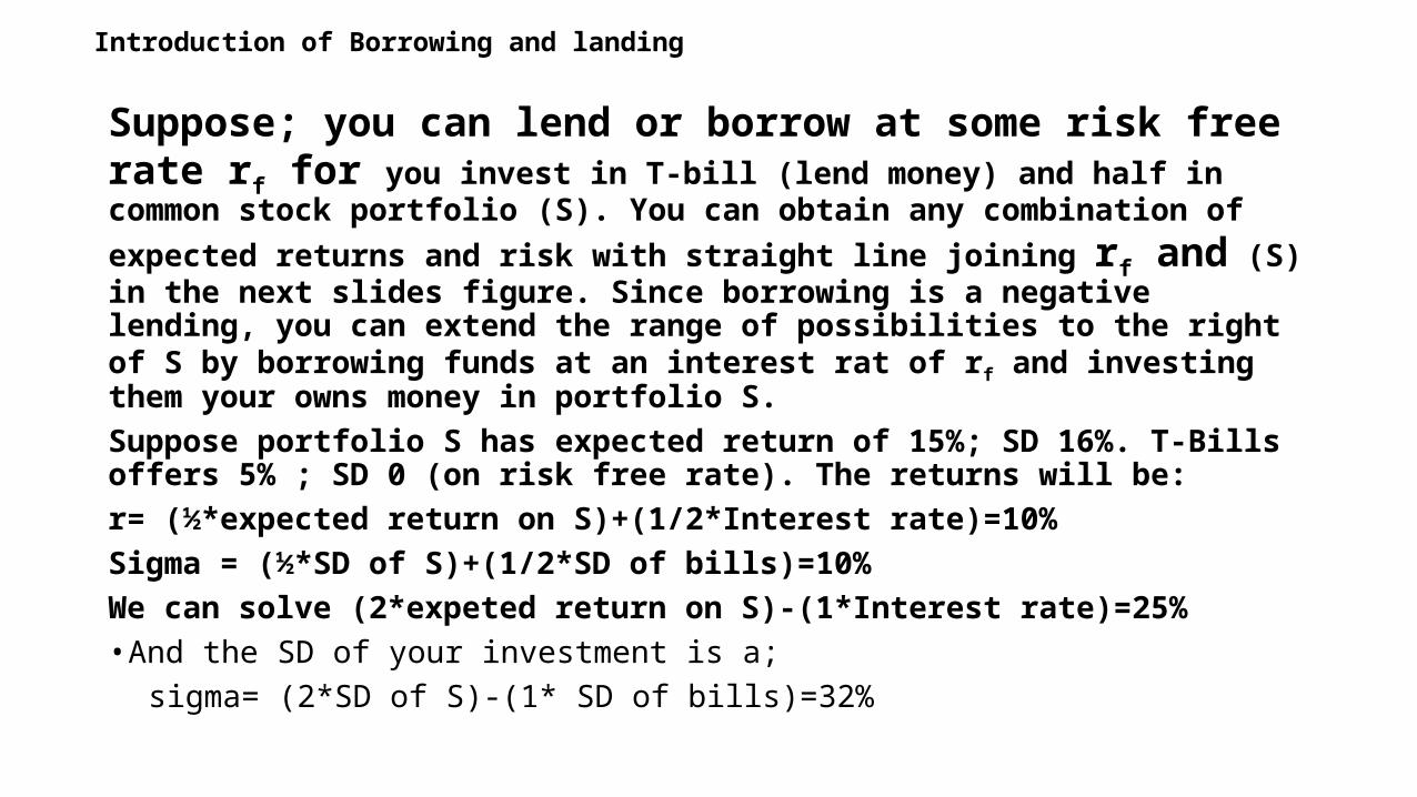
Introduction of Borrowing and landing

Suppose; you can lend or borrow at some risk free rate rf for you invest in T-bill (lend money) and half in common stock portfolio (S). You can obtain any combination of expected returns and risk with straight line joining rf and (S) in the next slides figure. Since borrowing is a negative lending, you can extend the range of possibilities to the right of S by borrowing funds at an interest rat of rf and investing them your owns money in portfolio S.Suppose portfolio S has expected return of 15%; SD 16%. T-Bills offers 5% ; SD 0 (on risk free rate). The returns will be:r= (½*expected return on S)+(1/2*Interest rate)=10%Sigma = (½*SD of S)+(1/2*SD of bills)=10%We can solve (2*expeted return on S)-(1*Interest rate)=25%• And the SD of your investment is a;

sigma= (2*SD of S)-(1* SD of bills)=32%

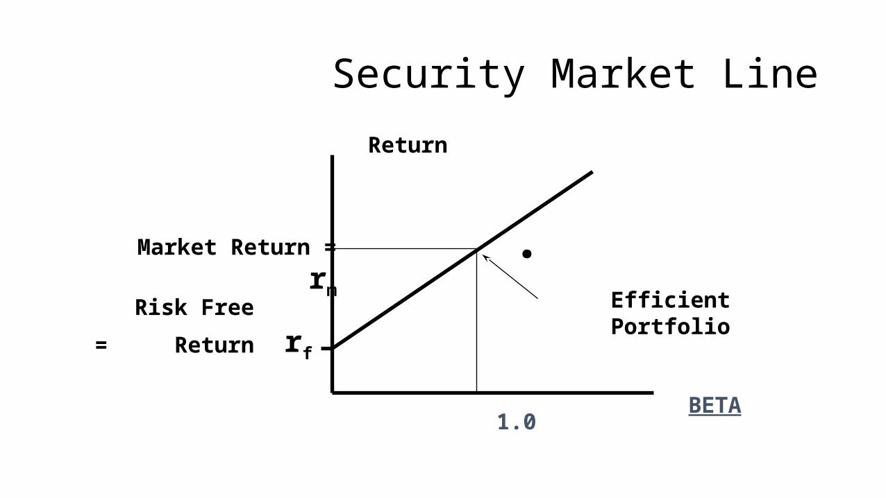
Security Market LineReturn

BETA

.rf

Risk Free Return=

Market Return = rm Efficient Portfolio

1.0

Security Market LineReturn

BETA

rf

Risk Free Return=

Market Return = rm

1.0

Security Market Line (SML)

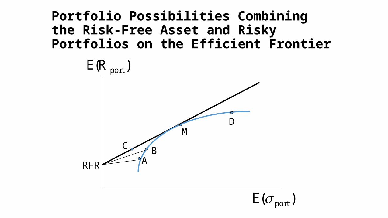
Portfolio Possibilities Combining the Risk-Free Asset and Risky Portfolios on the Efficient Frontier

)E( ports

)E(R port

RFR

MC

AB

D

Portfolio Possibilities Combining the Risk-Free Asset and Risky Portfolios on the

Efficient Frontier

RFR

M

CML

Borrowing

Lending

Testing the CAPMAvg Risk Premium

1931-65

Portfolio Beta1.0

SML30

20

10

0

Investors

Market Portfolio

Beta vs. Average Risk Premium

Testing the CAPMAvg Risk Premium

1966-91

Portfolio Beta1.0

SML

30

20

10

0

Investors

Market Portfolio

Beta vs. Average Risk Premium

Review of CAPM• Investor likes high expected return and low SD• Common Stock portfolios that offer the highest expected return for a

given SD known efficient portfolio• Investor attitude is important• Best efficient portfolio depends on investor’s assessment of expected

returns, SD and correlations• Do not look at the risk of individual asset rather go on portfolio risk

What if a stock did not lie on the security market line• Imagine that you encounter stock A which is lying beta.5 and away

from security line. You probably not as it is risky as well as giving you less returns

• If beta is 1.5 for another security B, what would you do, if, it is away from security line

expected risk premium on stock= beta*expected risk premium on market

r= rf= B(rm-rf)

Some alternative theories • Arbitrage pricing theory (APT)

CHAPTER 9 – The Capital Asset Pricing Model (CAPM)9 - 37

Alternative Asset Pricing ModelsThe Arbitrage Pricing Theory – the Model

• Underlying factors represent broad economic forces which are inherently unpredictable.

• Where:• ERi = the expected return on security i• a0 = the expected return on a security with zero systematic risk• bi = the sensitivity of security i to a given risk factor• Fi = the risk premium for a given risk factor

• The model demonstrates that a security’s risk is based on its sensitivity to broad economic forces.

... 11110 niniii FbFbFbaER [9-10]

CHAPTER 9 – The Capital Asset Pricing Model (CAPM)9 - 38

Alternative Asset Pricing ModelsThe Arbitrage Pricing Theory – Challenges

• Underlying factors represent broad economic forces which are inherently unpredictable.

• Ross and Roll identify five systematic factors:1. Changes in expected inflation2. Unanticipated changes in inflation3. Unanticipated changes in industrial production4. Unanticipated changes in the default-risk premium5. Unanticipated changes in the term structure of interest rates

• Clearly, something that isn’t forecast, can’t be used to price securities today…they can only be used to explain prices after the fact.

39

Arbitrage Pricing Theory• APT background• The APT model• Comparison of the CAPM and the APT

40

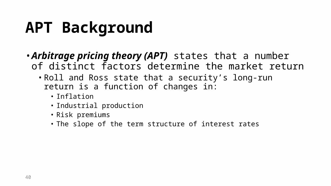
APT Background• Arbitrage pricing theory (APT) states that a number of distinct factors

determine the market return• Roll and Ross state that a security’s long-run return is a function of changes in:

• Inflation• Industrial production• Risk premiums• The slope of the term structure of interest rates

41

APT Background (cont’d)• Not all analysts are concerned with the same set of economic

information• A single market measure such as beta does not capture all the information

relevant to the price of a stock

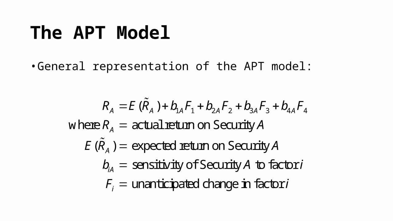
The APT Model• General representation of the APT model:

1 1 2 2 3 3 4 4( )where actual return on Security

( ) expected return on Security sensitivity of Security to factor unanticipated change in factor

A A A A A A

A

A

iA

i

R E R b F b F b F b FR A

E R Ab A iF i

APT1 1 2 2 3 3

1 1 1 2 2 2 3 3 3

1 1 2 2 3 3 1 1 2 2 3 3

Fixed Random

(Notice that the security index "A" has been ign

( )

( ) [ ( )] [ ( )] [ ( )]

( ) ( ) ( ) ( )

R E R F F F

R E R R E R R E R R E R

R E R E R E R E R R R R

ored for clarity purposes)

44

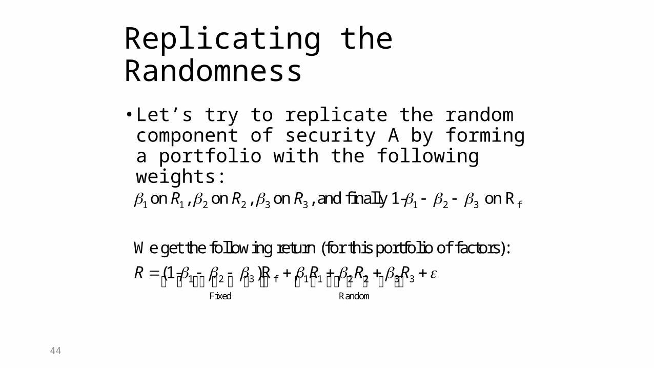
Replicating the Randomness• Let’s try to replicate the random component of

security A by forming a portfolio with the following weights:

1 1 2 2 3 3 1 2 3 f

1 2 3 f 1 1 2 2 3 3

Fixed Random

on , on , on , and finally 1- on R

We get the following return (for this portfolio of factors):(1- )R

R R R

R R R R

45

Key Point in Reasoning• Since we were able to match the random

components exactly, the only terms that differ at this point are the fixed components.

• But if one fixed component is larger than the other, arbitrage profits are possible by investing in the highest yielding security (either A or the portfolio of factors) while short-selling the other (being “long” in one and “short” in the other will assure an exact cancellation of the random terms).

46

•Therefore the fixed components MUST BE THE SAME for security A and the portfolio of factors created, otherwise unlimited profits would be possible.So we have:

1 1 2 2 3 3 1 2 3 f

f 1 1 f 2 2 f 2 3 f

( ) ( ) ( ) ( ) (1- )R

Rearranging terms yields:

( ) R [ ( ) R ] [ ( ) R ] [ ( ) R ]

E R E R E R E R

E R E R E R E R

47

Comparison of the CAPM and the APT• The CAPM’s market portfolio is difficult to construct:

• Theoretically all assets should be included (real estate, gold, etc.)• Practically, a proxy like the S&P 500 index is used

• APT requires specification of the relevant macroeconomic factors

48

Comparison of the CAPM and the APT (cont’d)• The CAPM and APT complement each other rather than compete

• Both models predict that positive returns will result from factor sensitivities that move with the market and vice versa

Arbitrage pricing theory (APT)Basic concept of CAPM is to use of portfolio effientlyStephen Rosss has it own theory in shape of APTAPT does not ask about which portfolio is efficient, instead, it starts by assuming that each stock’s return depends partly on pervasive macroeconomic influence or factors and partly on noise- events that are unique to that company

Thank you very much for your time and discussion