Embed Size (px)
Citation preview

The "Checklist"> 10. Execution> Order scheduling
Order scheduling
Goal: find the optimal trading schedule for a parent order of size ∆hparent
ht−start
initial position
ht−end = h
t−start+ ∆hparent?
terminal position
where• tstart = “now”;• tend = “as soon as possible, considering the adverse impact of ourtrading”.
Going forward, we analyze order scheduling in volume time (1.104), see Table10.4, and we consider implicit the conditioning on the current information.
ARPM - Advanced Risk and Portfolio Management - arpm.co This update: Apr-05-2017 - Last update
The "Checklist"> 10. Execution> Order schedulingP&L computation
Trading P&L decomposition
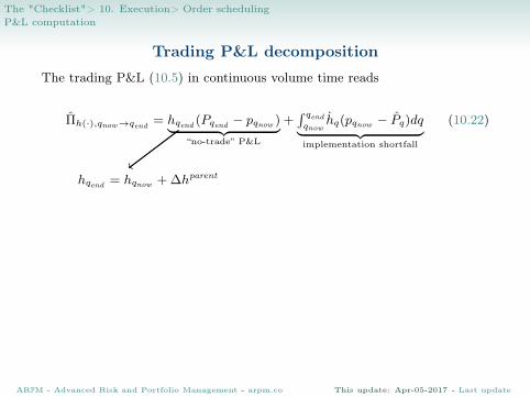
The trading P&L (10.5) in continuous volume time reads
Πh(·),qnow→qend = hqend (Pqend − pqnow )︸ ︷︷ ︸“no-trade” P&L
+∫ qendqnow
hq(pqnow − Pq)dq︸ ︷︷ ︸implementation shortfall
(10.22)
hqend = hqnow + ∆hparent
ARPM - Advanced Risk and Portfolio Management - arpm.co This update: Apr-05-2017 - Last update

The "Checklist"> 10. Execution> Order schedulingP&L computation
Trading P&L decomposition
The trading P&L (10.5) in continuous volume time reads
Πh(·),qnow→qend = hqend (Pqend − pqnow )︸ ︷︷ ︸“no-trade” P&L
+∫ qendqnow
hq(pqnow − Pq)dq︸ ︷︷ ︸implementation shortfall
(10.22)
hqend = hqnow + ∆hparent = 0 liquidation (11.37)
ARPM - Advanced Risk and Portfolio Management - arpm.co This update: Apr-05-2017 - Last update

The "Checklist"> 10. Execution> Order schedulingP&L computation
Market impact P&L
The trading P&L (10.5) in continuous volume time reads
Πh(·),qnow→qend = hqend (Pqend − pqnow )︸ ︷︷ ︸“no-trade” P&L
+∫ qendqnow
hq(pqnow − Pq)dq︸ ︷︷ ︸implementation shortfall
(10.22)
hqend = hqnow + ∆hparent
⇓ Market impact model (10.16)
Market impact P&L
Πh(·),qnow→qend = hqend
∫ qend
qnow
b(qend − q)f(hq) dq + σhqendBqend−qnow︸ ︷︷ ︸“no-trade” P&L
−∫ qend
qnow
hqg(hq)dq −∫ qend
qnow
hq(∫ qqnow
b(q − s)f(hs) ds)dq − σ∫ qend
qnow
hqBq−qnow dq︸ ︷︷ ︸implementation shortfall
(10.23)
ARPM - Advanced Risk and Portfolio Management - arpm.co This update: Apr-05-2017 - Last update
The "Checklist"> 10. Execution> Order schedulingP&L evaluation
Market impact P&L: distribution
Πh(·),qnow→qend ∼ N (?, ?)
ARPM - Advanced Risk and Portfolio Management - arpm.co This update: Apr-05-2017 - Last update
The "Checklist"> 10. Execution> Order schedulingP&L evaluation
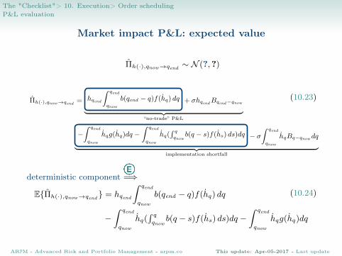
Market impact P&L: expected value
Πh(·),qnow→qend ∼ N (?, ?)
(10.23)Πh(·),qnow→qend = hqend
∫ qend
qnow
b(qend − q)f(hq) dq + σhqendBqend−qnow︸ ︷︷ ︸“no-trade” P&L
−∫ qend
qnow
hqg(hq)dq −∫ qend
qnow
hq(∫ qqnow
b(q − s)f(hs) ds)dq − σ∫ qend
qnow
hqBq−qnow dq︸ ︷︷ ︸implementation shortfall
deterministic component =⇒
E{Πh(·),qnow→qend } = hqend
∫ qend
qnow
b(qend − q)f(hq) dq
−∫ qend
qnow
hq(∫ qqnow
b(q − s)f(hs) ds)dq −∫ qend
qnow
hqg(hq)dq
(10.24)
ARPM - Advanced Risk and Portfolio Management - arpm.co This update: Apr-05-2017 - Last update

The "Checklist"> 10. Execution> Order schedulingP&L evaluation
Market impact P&L: variance
Πh(·),qnow→qend ∼ N (?, ?)
(10.23)Πh(·),qnow→qend = hqend
∫ qend
qnow
b(qend − q)f(hq) dq + σhqendBqend−qnow︸ ︷︷ ︸“no-trade” P&L
−∫ qend
qnow
hqg(hq)dq −∫ qend
qnow
hq(∫ qqnow
b(q − s)f(hs) ds)dq − σ
∫ qend
qnow
hqBq−qnow dq︸ ︷︷ ︸implementation shortfall
stochastic component =⇒ V{Πh(·),qnow→qend } = σ2∫ qendqnow
h2qdq (1)(10.25)
The variance is model-independent
• Trade at the end ⇒ large variance• Trade at the beginning ⇒ no variance
ARPM - Advanced Risk and Portfolio Management - arpm.co This update: Apr-05-2017 - Last update

The "Checklist"> 10. Execution> Order schedulingP&L optimization
Two-step mean-variance optimization
Step 1: hλ (·) ≡ argmaxh(·)∈C
(E{Πh(·),qnow→qend } − λV{Πh(·),qnow→qend })
(10.26)set of constraints
ARPM - Advanced Risk and Portfolio Management - arpm.co This update: Apr-05-2017 - Last update

The "Checklist"> 10. Execution> Order schedulingP&L optimization
Two-step mean-variance optimization
Step 1: hλ (·) ≡ argmaxh(·)∈C
(E{Πh(·),qnow→qend } − λV{Πh(·),qnow→qend })
(10.26)set of constraints
Full execution requirement
C : {{hq}q∈[qnow ,qend ) such that∫ qendqnow
hqdq = ∆hparent} (10.27)
Full execution
ARPM - Advanced Risk and Portfolio Management - arpm.co This update: Apr-05-2017 - Last update

The "Checklist"> 10. Execution> Order schedulingP&L optimization
Two-step mean-variance optimization
Step 1: hλ (·) ≡ argmaxh(·)∈C
(E{Πh(·),qnow→qend }−λV{Πh(·),qnow→qend }) (10.26)
set of constraints
Full execution requirement
C : {{hq}q∈[qnow ,qend ) such that∫ qendqnow
hqdq = ∆hparent} (10.27)
Full execution
Step 2: h∗ (·) ≡ argmaxλ
satis(hλ (·)) (10.29)
best trajectory index ofsatisfaction (7a.5)
ARPM - Advanced Risk and Portfolio Management - arpm.co This update: Apr-05-2017 - Last update
The "Checklist"> 10. Execution> Order schedulingP&L optimization
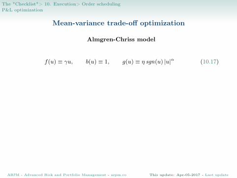
Mean-variance trade-off optimization
Almgren-Chriss model
f(u) ≡ γu, b(u) ≡ 1, g(u) ≡ η sgn(u) |u|α (10.17)
ARPM - Advanced Risk and Portfolio Management - arpm.co This update: Apr-05-2017 - Last update
The "Checklist"> 10. Execution> Order schedulingP&L optimization
Mean-variance trade-off optimization
Almgren-Chriss model
market impact function
f(u) ≡ γu , b(u) ≡ 1, g(u) ≡ η sgn(u) |u|α (10.17)
positive
ARPM - Advanced Risk and Portfolio Management - arpm.co This update: Apr-05-2017 - Last update

The "Checklist"> 10. Execution> Order schedulingP&L optimization
Mean-variance trade-off optimization
Almgren-Chriss model
market impact decay kernel
f(u) ≡ γu, b(u) ≡ 1 , g(u) ≡ η sgn(u) |u|α (10.17)
ARPM - Advanced Risk and Portfolio Management - arpm.co This update: Apr-05-2017 - Last update

The "Checklist"> 10. Execution> Order schedulingP&L optimization
Mean-variance trade-off optimization
Almgren-Chriss model
slippage
f(u) ≡ γu, b(u) ≡ 1, g(u) ≡ η sgn(u) |u|α (10.17)
positive α = 1
ARPM - Advanced Risk and Portfolio Management - arpm.co This update: Apr-05-2017 - Last update

The "Checklist"> 10. Execution> Order schedulingP&L optimization
Mean-variance trade-off optimization
Almgren-Chriss model
f(u) ≡ γu, b(u) ≡ 1, g(u) ≡ η sgn(u) |u|α (10.17)
• full execution requirement (10.27)
• total liquidation (11.37), i.e. hqend = 0
The solution of the mean-variance trade-off (10.26) is
hλ(q) = hqnow
sinh(√
λησ(qend − q))
sinh(√
λησ(qend − qnow ))
(10.30)
• the trajectories {hλ(·)}λ are monotonically decreasing from hqnow to 0
• ληdetermines the speed of trading
ARPM - Advanced Risk and Portfolio Management - arpm.co This update: Apr-05-2017 - Last update
The "Checklist"> 10. Execution> Order schedulingP&L optimization
Mean-variance trade-off optimization
Almgren-Chriss model
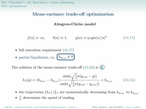
f(u) ≡ γu, b(u) ≡ 1, g(u) ≡ η sgn(u) |u|α (10.17)
• full execution requirement (10.27)
• partial liquidation, i.e. hqend 6= 0
The solution of the mean-variance trade-off (10.26) is
hλ(q) = (hqnow − hqend )sinh(
√λησ(qend − q))
sinh(√
λησ(qend − qnow ))
+ hqend (10.31)
• the trajectories {hλ(·)}λ are monotonically decreasing from hqnow to• λ
ηdetermines the speed of trading
hqend
ARPM - Advanced Risk and Portfolio Management - arpm.co This update: Apr-05-2017 - Last update

The "Checklist"> 10. Execution> Order schedulingP&L optimization
Trading trajectories in the Almgren-Chriss model
• volume time interval: [0, 1)
• initial position: hqnow = 100
• final position: hqend = 90
• "daily" parameters: η = 0.135, σ = 1.57
• λ = 0, 0.3, 1, 5
ARPM - Advanced Risk and Portfolio Management - arpm.co This update: Apr-05-2017 - Last update
The "Checklist"> 10. Execution> Order schedulingP&L optimization
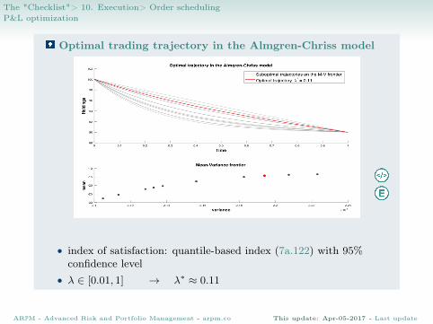
Optimal trading trajectory in the Almgren-Chriss model
• index of satisfaction: quantile-based index (7a.122) with 95%confidence level
• λ ∈ [0.01, 1] → λ∗ ≈ 0.11
ARPM - Advanced Risk and Portfolio Management - arpm.co This update: Apr-05-2017 - Last update

The "Checklist"> 10. Execution> Order schedulingP&L quasi-optimal distribution
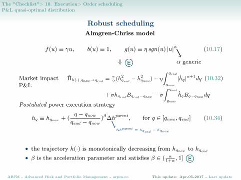
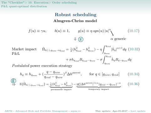
Robust schedulingAlmgren-Chriss model
f(u) ≡ γu, b(u) ≡ 1, g(u) ≡ η sgn(u) |u|α (10.17)
α generic⇓
Πh(·),qnow→qend = γ2
(h2qend − h
2qnow )− η
∫ qend
qnow
|hq|α+1dq
+ σhqendBqend−qnow − σ∫ qend
qnow
hqBq−qnow dq
Market impactP&L
(10.32)
ARPM - Advanced Risk and Portfolio Management - arpm.co This update: Apr-05-2017 - Last update
The "Checklist"> 10. Execution> Order schedulingP&L quasi-optimal distribution
Robust schedulingAlmgren-Chriss model
f(u) ≡ γu, b(u) ≡ 1, g(u) ≡ η sgn(u) |u|α (10.17)
α generic⇓
Πh(·),qnow→qend = γ2
(h2qend − h
2qnow )− η
∫ qend
qnow
|hq|α+1dq
+ σhqendBqend−qnow − σ∫ qend
qnow
hqBq−qnow dq
Market impactP&L
(10.32)
Postulated power execution strategy
hq ≡ hqnow + (q − qnowqend − qnow
)β∆hparent , for q ∈ [qnow , qend ] (10.34)
∆hparent ≡ hqend− hqnow
• the trajectory h(·) is monotonically decreasing from hqnow to hqend• β is the acceleration parameter and satisfies β ∈ ( α
1+α, 1]
ARPM - Advanced Risk and Portfolio Management - arpm.co This update: Apr-05-2017 - Last update
The "Checklist"> 10. Execution> Order schedulingP&L quasi-optimal distribution
Robust schedulingAlmgren-Chriss model
f(u) ≡ γu, b(u) ≡ 1, g(u) ≡ η sgn(u) |u|α (10.17)
α generic⇓
Πh(·),qnow→qend = γ2
(h2qend − h
2qnow )− η
∫ qend
qnow
|hq|α+1dq
+ σhqendBqend−qnow − σ∫ qend
qnow
hqBq−qnow dq
Market impactP&L
(10.32)
Postulated power execution strategy
hq ≡ hqnow + (q − qnowqend − qnow
)β∆hparent , for q ∈ [qnow , qend ] (10.34)
⇒ E{Πh(·),qnow→qend } = γ2
(h2qend − h
2qnow )︸ ︷︷ ︸
permanent impact
− ηξ|∆hparent |1+α(qend − qnow )−α︸ ︷︷ ︸temporary impact
(10.36)
ξ ≡ βα+1/(β + βα − α) > 0
• Execute faster (β = 0+) ⇒ lower expected value• Execute slower (β = 1) ⇒ higher expected value
ARPM - Advanced Risk and Portfolio Management - arpm.co This update: Apr-05-2017 - Last update
The "Checklist"> 10. Execution> Order schedulingP&L quasi-optimal distribution
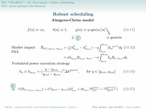
Robust schedulingAlmgren-Chriss model
f(u) ≡ γu, b(u) ≡ 1, g(u) ≡ η sgn(u) |u|α (10.17)
α generic⇓
Πh(·),qnow→qend = γ2
(h2qend − h
2qnow )− η
∫ qend
qnow
|hq|α+1dq
+ σhqendBqend−qnow − σ∫ qend
qnow
hqBq−qnow dq
Market impactP&L
(10.32)
Postulated power execution strategy
hq ≡ hqnow + (q − qnowqend − qnow
)β∆hparent , for q ∈ [qnow , qend ] (10.34)
⇒ V{Πh(·),qnow→qend } = σ2(qend − qnow )(h2qnow + 2hqnow
∆hparent
β+1+ (∆hparent )2
2β+1) (10.37)
ARPM - Advanced Risk and Portfolio Management - arpm.co This update: Apr-05-2017 - Last update