Chapter 9

Uniprocessor Scheduling

In a multiprogramming system, multiple pro-

cesses are kept in the main memory. Each

process alternates between using the proces-

sor, and waiting for an I/O device or another

event to occur. Every effort is made to keep

the processor busy.

The key for such a system to work is schedul-

ing, namely, assign processes to the processor

over time, such that certain system objectives

will be met. These may include response time,

throughput, and processor efficiency.

In many systems, such an activity is further

broken into short-, medium-, and long-term

scheduling, relative to the time scale for these

activities.

1

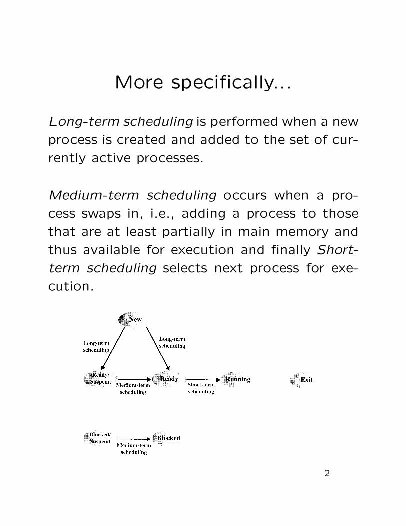
More specifically...

Long-term scheduling is performed when a new

process is created and added to the set of cur-

rently active processes.

Medium-term scheduling occurs when a pro-

cess swaps in, i.e., adding a process to those

that are at least partially in main memory and

thus available for execution and finally Short-

term scheduling selects next process for exe-

cution.

2

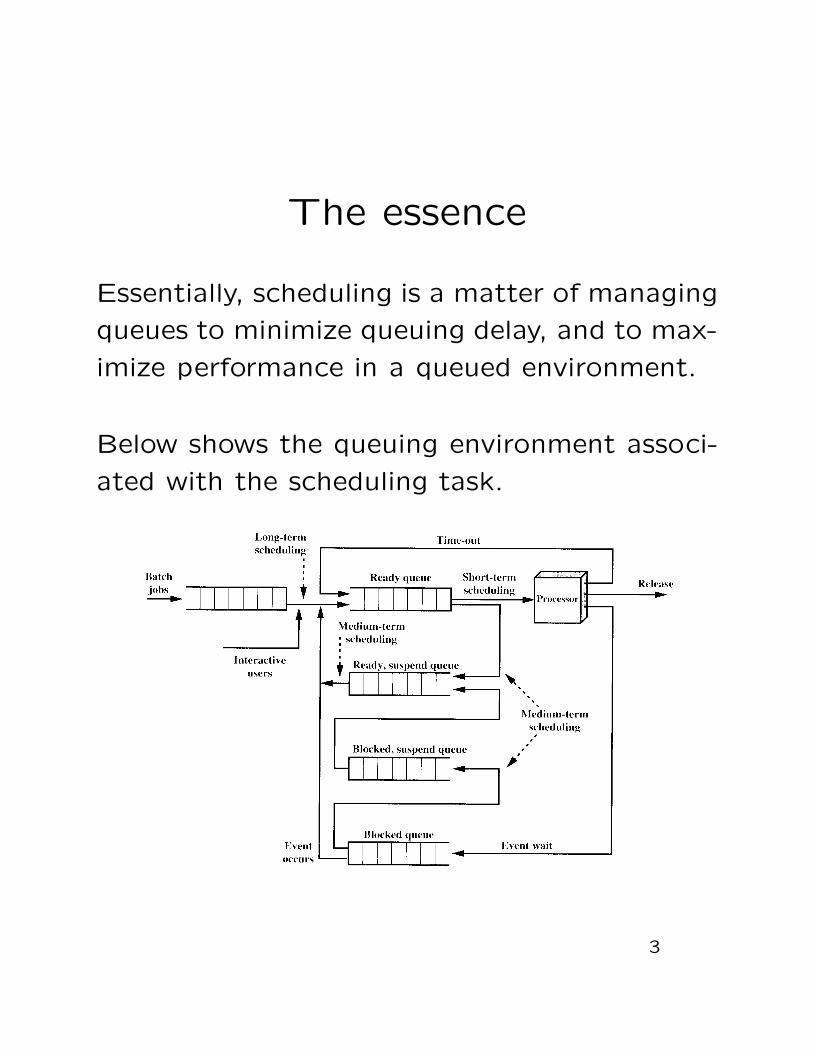
The essence

Essentially, scheduling is a matter of managing

queues to minimize queuing delay, and to max-

imize performance in a queued environment.

Below shows the queuing environment associ-

ated with the scheduling task.

3

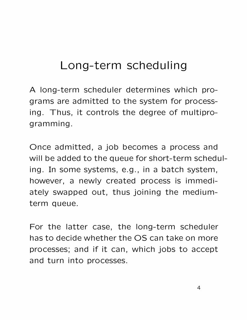
Long-term scheduling

A long-term scheduler determines which pro-

grams are admitted to the system for process-

ing. Thus, it controls the degree of multipro-

gramming.

Once admitted, a job becomes a process and

will be added to the queue for short-term schedul-

ing. In some systems, e.g., in a batch system,

however, a newly created process is immedi-

ately swapped out, thus joining the medium-

term queue.

For the latter case, the long-term scheduler

has to decide whether the OS can take on more

processes; and if it can, which jobs to accept

and turn into processes.

4

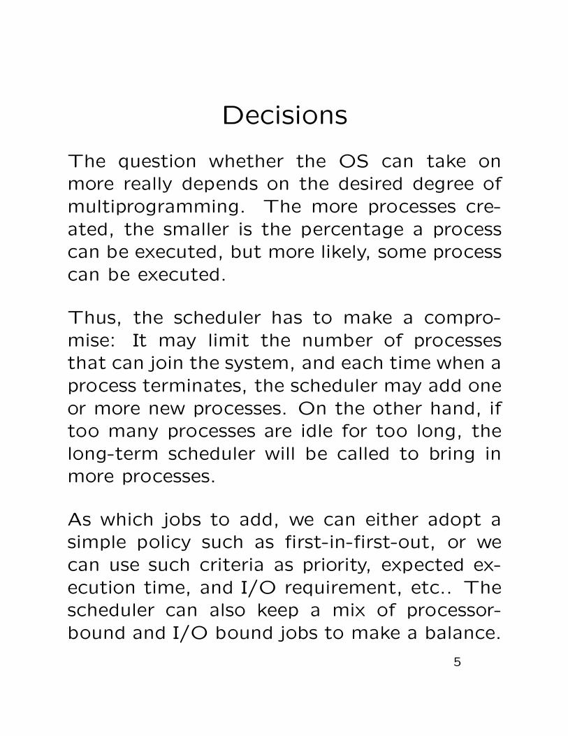
Decisions

The question whether the OS can take on

more really depends on the desired degree of

multiprogramming. The more processes cre-

ated, the smaller is the percentage a process

can be executed, but more likely, some process

can be executed.

Thus, the scheduler has to make a compro-

mise: It may limit the number of processes

that can join the system, and each time when a

process terminates, the scheduler may add one

or more new processes. On the other hand, if

too many processes are idle for too long, the

long-term scheduler will be called to bring in

more processes.

As which jobs to add, we can either adopt a

simple policy such as first-in-first-out, or we

can use such criteria as priority, expected ex-

ecution time, and I/O requirement, etc.. The

scheduler can also keep a mix of processor-

bound and I/O bound jobs to make a balance.

5

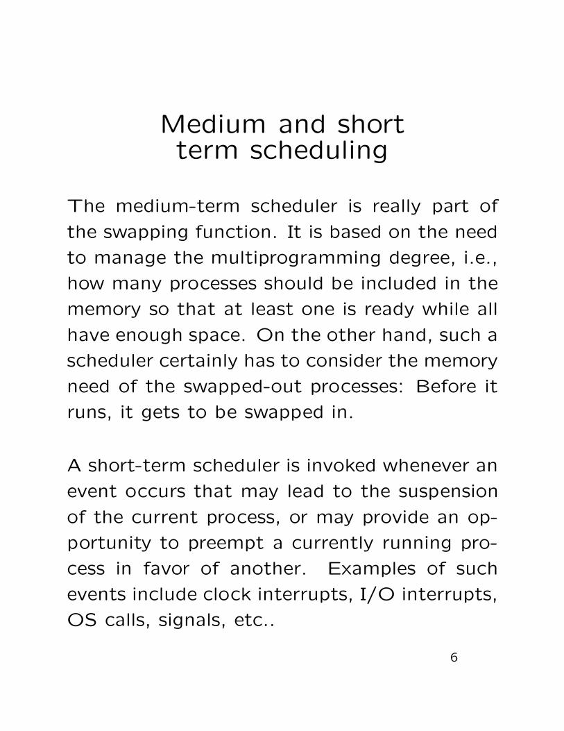
Medium and shortterm scheduling

The medium-term scheduler is really part of

the swapping function. It is based on the need

to manage the multiprogramming degree, i.e.,

how many processes should be included in the

memory so that at least one is ready while all

have enough space. On the other hand, such a

scheduler certainly has to consider the memory

need of the swapped-out processes: Before it

runs, it gets to be swapped in.

A short-term scheduler is invoked whenever an

event occurs that may lead to the suspension

of the current process, or may provide an op-

portunity to preempt a currently running pro-

cess in favor of another. Examples of such

events include clock interrupts, I/O interrupts,

OS calls, signals, etc..

6

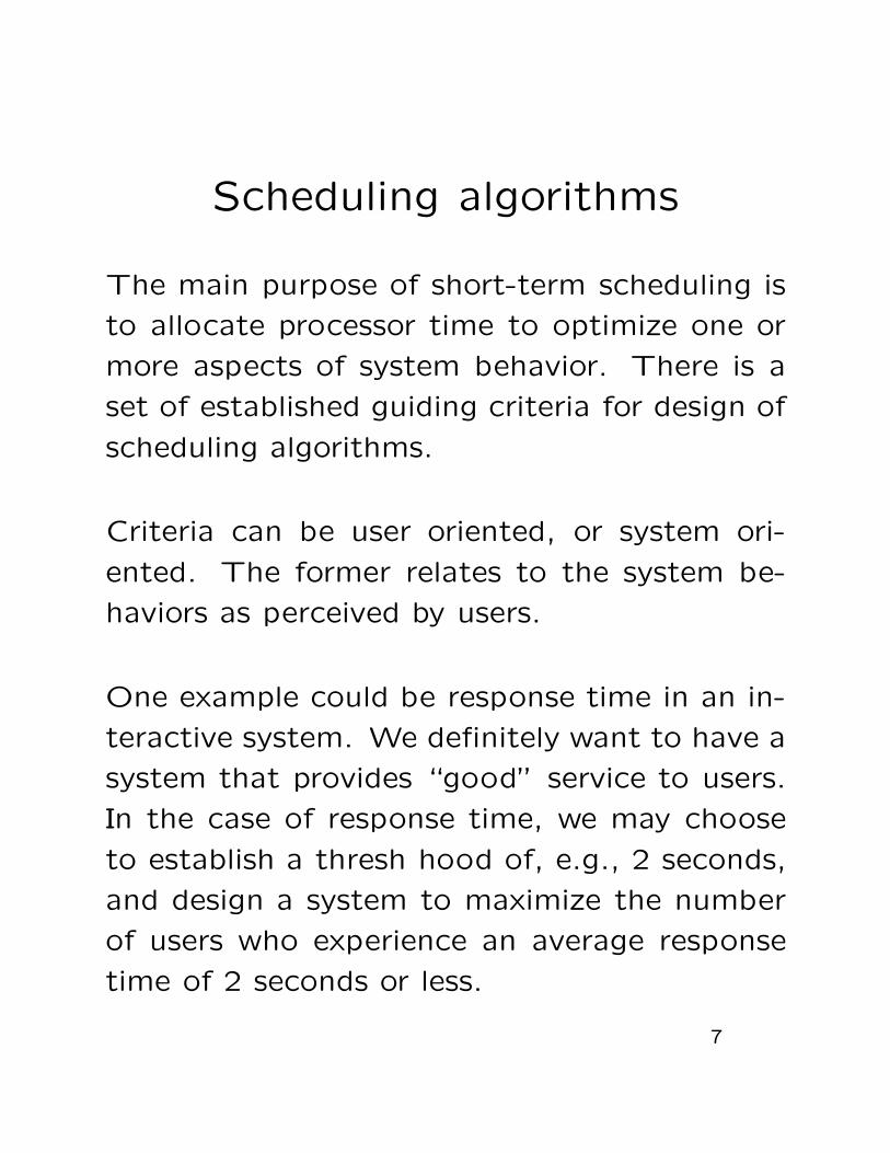
Scheduling algorithms

The main purpose of short-term scheduling is

to allocate processor time to optimize one or

more aspects of system behavior. There is a

set of established guiding criteria for design of

scheduling algorithms.

Criteria can be user oriented, or system ori-

ented. The former relates to the system be-

haviors as perceived by users.

One example could be response time in an in-

teractive system. We definitely want to have a

system that provides “good” service to users.

In the case of response time, we may choose

to establish a thresh hood of, e.g., 2 seconds,

and design a system to maximize the number

of users who experience an average response

time of 2 seconds or less.

7

The other side of the coin

System oriented criteria focus on effective and

efficient utilization of the processor. An exam-

ple could be throughput, i.e., the rate of suc-

cessfully completed processes, which we cer-

tainly want to maximize.

User-oriented criteria are important for all sys-

tems, but it is not as important for a single-

user system, as long as users are happy. In

most systems, “short” response time is a crit-

ical requirement.

8

Another dimension

Criteria can also be categorized as performance

related, or not. Performance related criteria

are usually quantitative, and can be measured.

Response time and throughput are such exam-

ples.

Criteria that are not performance related are

just the opposite. One example could be pre-

dictability, namely, the expectation that the

system will exhibit to the users the same char-

acteristics over time, independent of anything

else.

For example, the WebReg should have the same

interface no matter what we put it. Obviously,

its measurement is not as straightforward as

the first two.

Assignment: Go through the scheduling cri-

teria summary table, i.e., Table 9.2.

9

Using priorities

In many systems, each process is assigned a

priority, and the scheduler always selects a pro-

cess of higher priority over one of lower priority.

This idea can be implemented by providing

a set of Ready queues, one for each prior-

ity. When picking up things, the scheduler will

start with the highest-priority queue. If it is

not empty, a process will be selected by using

certain policy. Otherwise, a lower queue will

be tried, etc..

One obvious consequence is that lower-priority

processes may suffer from starvation, if higher

priority processes keep on coming. A possi-

ble solution is to reflect the age or execution

history into the priority of a process.

10

Various scheduling policies

There are many of them, such as first-come-

first-served, round-robin, shortest process first,

shortest remaining time, feedback, etc..

For all these policies, a selection function is

used to select a process as the next one for

execution, based on either priority, resource

requirement, or the execution characteristics

such as w, time spent in the system so far;

e, time spent in execution so far; and s, total

estimated service time required by the process.

11

Question: What should happen when the se-

lection function is carried out?

Answer: It depends on the decision mode. If

it is non-preemptive, then a running process

will continue to execute until and unless it ter-

minates, or gets blocked for whatever reason.

On the other hand, if it is preemptive, then,

the currently running process may be inter-

rupted and put back to the ready state, when,

e.g., a new process is created, an interrupt oc-

curs that moves a blocked process back into

the ready state, or even periodically one such

as a clock interrupt for an animation program.

Preemptive mode causes more overhead but

may provide better service.

12

First come, first serve

This FCFS policy is a strict queuing scheme.

As each process becomes ready, a medium sched-

uler puts it into the Ready queue. When the

current process is taken off the processor, the

process located at the front end of the queue

will be selected to run.

To compare this strategy with the others, we

have to know the arrival time, and the service

time. We also define the turnaround time to

be the total time the process spends in the

system, namely, the sum of waiting time plus

service time.

Another telling quantity is the normalized turn-

around time, i.e., the ratio of turnaround time

to service time. The closer this ratio is to 1,

the better.

13

What can we say about it?

Some data shows that the FCFS policy works

better for longer processes than shorter ones:

When a short process comes after a much longer

one, it may take a while for it to be picked up.

Another issue with the FCFS policy is that it

tends to favor processor-bound processes over

I/O-bound processes: when a processor-bound

process is running, all the I/O-bound ones have

to wait. Some of them could be in the I/O

queue, or may move back to the Ready queue

while the processor is working. Thus, most of

the I/O devices may be idle, even though they

potentially have work to do.

When the processor-bound process stops its

execution for whatever reason, the I/O-bound

processes will be picked up, but soon get blocked

again on I/O events.

Thus, FCFS may lead to a low efficiency.

14

Round robin

A simple way to reduce the penalty for the

shorter jobs under FCFS is to use a clock based

preemptive technique, e.g., using a Round robin

policy. A clock interrupt is generated at pe-

riodical intervals. When the interrupt occurs,

the current process is placed in the Ready queue,

and the next ready one is selected on a FCFS

basis. This is also referred to as time slicing.

The key design issue is the length of the time

slice. If this slice is very short, shorter pro-

cesses will move through the system quickly,

but the overhead involved in handling frequent

interrupt and performing dispatching functions

will become significant. Thus, too short a slice

should be avoided.

Homework: Problems 9.11 and 13.

15

A useful guide is...

that the slice should be a little bigger than the

time required for a typical interaction. If it

is less than this thresh hood, then most pro-

cesses will require at least two time slices to

complete. When the slice is longer than the

longest-running process, round robin degener-

ates to FCFS.

Although quite effective in a general purpose

time sharing system, or transaction processing

system, the Round robin policy tends to treat

I/O-bound processes unfairly. Since they tend

to use only a portion of the slice, then get

blocked for I/O operation; while a processor-

bound process usually uses a whole slice. This

may be resolved by using another queue to give

preference to those blocked I/O-bound pro-

cesses.

16

How to do it?

The Round Robin procedure goes like this: for

a given n processes, p0, p1, . . . , pn−1, the dis-

patcher will assign the processor to each pro-

cess approximately 1n slices (time quanta) for

every real-time unit.

When a new process arrives, it is added into

the rear end of the Ready queue with its arrival

time as a time stamp, and when the share of

the currently running process is used up, but

itself is not completed yet, this process will be

put back to the queue with a new time stamp,

the time when this round is done.

The dispatcher just picks the one that has

stayed in the queue the longest time, or the

one with the smallest time stamp, as the next

process to run.

It is clear that the appropriate data structure

should be the priority queue, which might be

implemented with a minHeap.

17

Shortest process next

This is also a non-preemptive policy that al-

ways picks up a process with the shortest ex-

pected execution time. It again can be man-

aged with a heap structure, (Still remember

this stuff?)

Under this policy, besides quicker response time

to shorter processes, overall performance is

also significantly increased. But, predictability

is reduced. We also have to at least estimate

the required processing time. Moreover, longer

processes might be starved.

In a production environment, the same job runs

many times, then some statistics may be col-

lected for future reference.

18

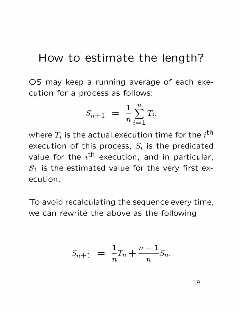
How to estimate the length?

OS may keep a running average of each exe-

cution for a process as follows:

Sn+1 =1

n

n∑

i=1

Ti,

where Ti is the actual execution time for the ith

execution of this process, Si is the predicated

value for the ith execution, and in particular,

S1 is the estimated value for the very first ex-

ecution.

To avoid recalculating the sequence every time,

we can rewrite the above as the following

Sn+1 =1

nTn +

n − 1

nSn.

19

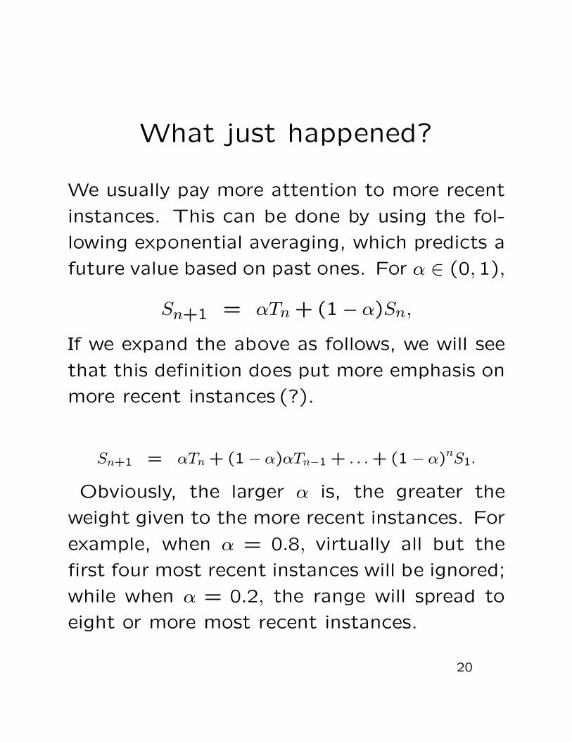
What just happened?

We usually pay more attention to more recent

instances. This can be done by using the fol-

lowing exponential averaging, which predicts a

future value based on past ones. For α ∈ (0,1),

Sn+1 = αTn + (1 − α)Sn,

If we expand the above as follows, we will see

that this definition does put more emphasis on

more recent instances (?).

Sn+1 = αTn + (1 − α)αTn−1 + . . . + (1 − α)nS1.

Obviously, the larger α is, the greater the

weight given to the more recent instances. For

example, when α = 0.8, virtually all but the

first four most recent instances will be ignored;

while when α = 0.2, the range will spread to

eight or more most recent instances.

20

Shortest remaining time

This policy is the preemptive version of the

previous SPN policy.

When it is time to choose, such a scheduler al-

ways chooses the process that has the shortest

expected remaining processing time.

Indeed, when a new process joins the Ready

queue, if it has a shorter execution time, com-

pared with the remaining execution time of the

current process, the scheduler will choose this

new process whenever it is ready.

As with the SPN policy, the user has to provide

with OS the estimated processing time infor-

mation, and the longer processes also have to

take a risk of starvation.

21

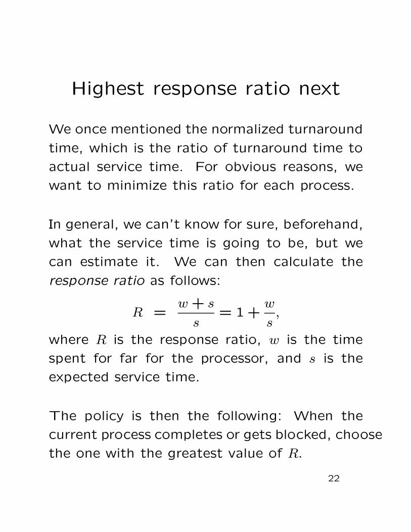
Highest response ratio next

We once mentioned the normalized turnaround

time, which is the ratio of turnaround time to

actual service time. For obvious reasons, we

want to minimize this ratio for each process.

In general, we can’t know for sure, beforehand,

what the service time is going to be, but we

can estimate it. We can then calculate the

response ratio as follows:

R =w + s

s= 1 +

w

s,

where R is the response ratio, w is the time

spent for far for the processor, and s is the

expected service time.

The policy is then the following: When the

current process completes or gets blocked, choose

the one with the greatest value of R.

22

What about it?

This policy considers both the total amount of

time a process has been in the system, and its

expected service time.

• A shorter process is favored, because of its

short service time, which leads to a larger

ratio;

• An aging process without service will also

be considered. Thus, those processes that

have been there for a while will not be ig-

nored, either.

As with the previous policies, estimation of ser-

vice time has to be provided.

23

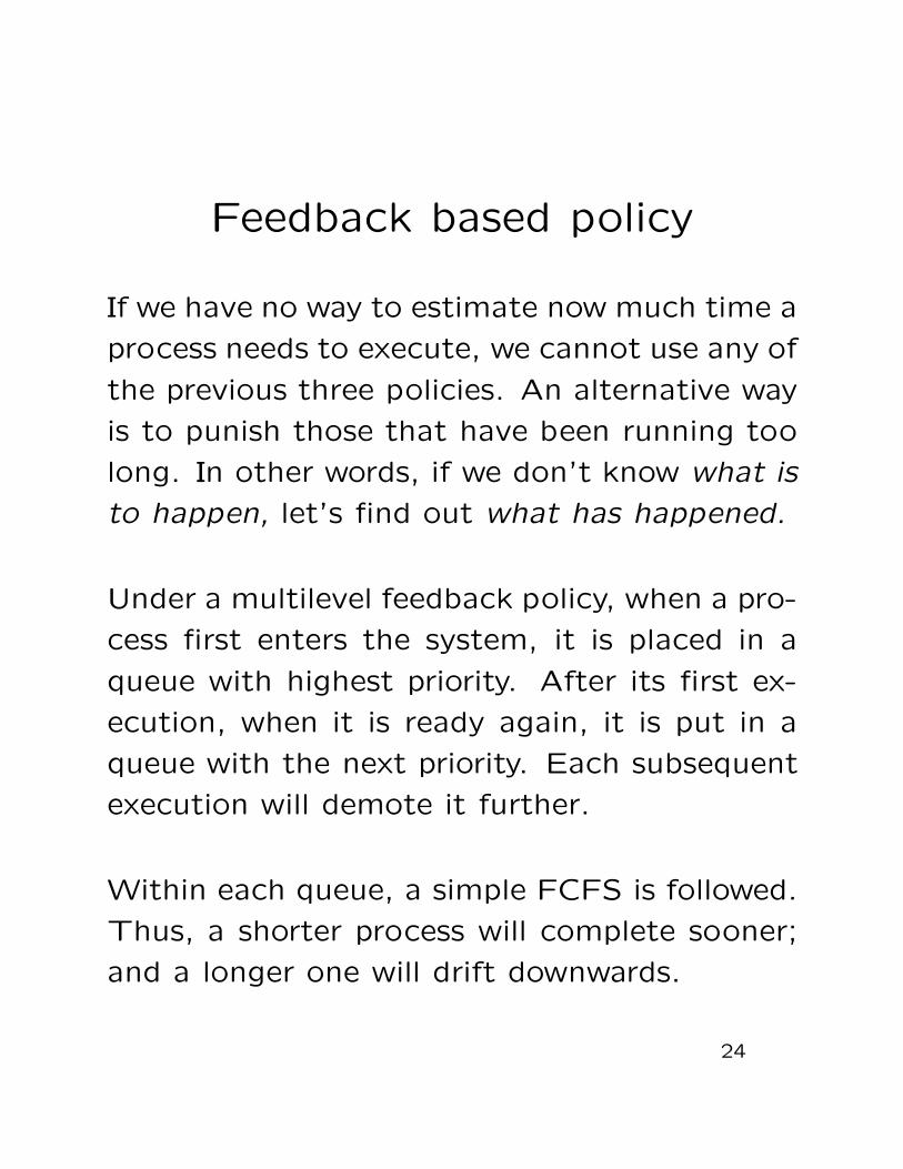
Feedback based policy

If we have no way to estimate now much time a

process needs to execute, we cannot use any of

the previous three policies. An alternative way

is to punish those that have been running too

long. In other words, if we don’t know what is

to happen, let’s find out what has happened.

Under a multilevel feedback policy, when a pro-

cess first enters the system, it is placed in a

queue with highest priority. After its first ex-

ecution, when it is ready again, it is put in a

queue with the next priority. Each subsequent

execution will demote it further.

Within each queue, a simple FCFS is followed.

Thus, a shorter process will complete sooner;

and a longer one will drift downwards.

24

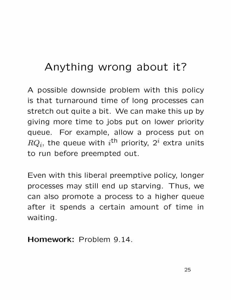
Anything wrong about it?

A possible downside problem with this policy

is that turnaround time of long processes can

stretch out quite a bit. We can make this up by

giving more time to jobs put on lower priority

queue. For example, allow a process put on

RQi, the queue with ith priority, 2i extra units

to run before preempted out.

Even with this liberal preemptive policy, longer

processes may still end up starving. Thus, we

can also promote a process to a higher queue

after it spends a certain amount of time in

waiting.

Homework: Problem 9.14.

25

26

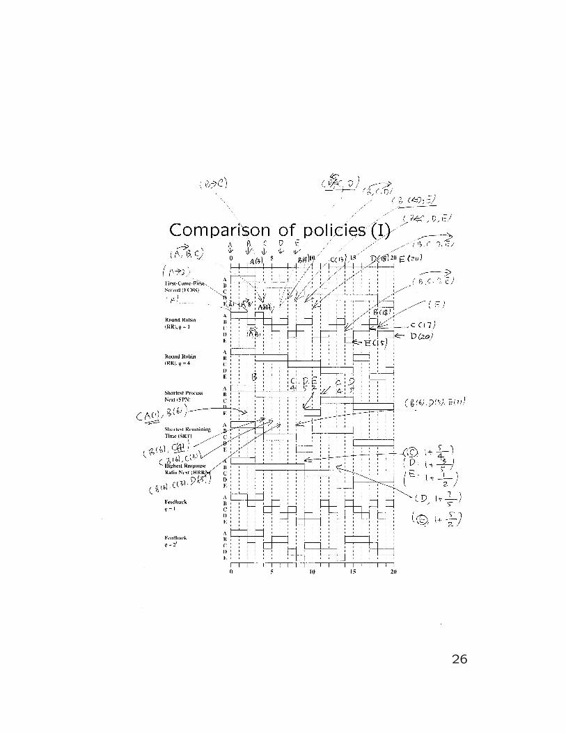
Comparison of policies (II)

Project: Have you checked out the project

page yet?

27

What is going on?

Use the Round Robin, with the size of the time

slot being 4, referred to as RR(4), as an exam-

ple, when process A comes at t = 0, no body

is waiting, thus it has the processor, and runs

for 3 units and gets out at t = 3.. Then B(2),

which came in at t = 2, jumps in and runs until

t = 7, when it rejoins the queue. Both B(7)

and C(4) are waiting, as C came in earlier at

t = 4, it will have the processor until t = 11.

Now, B(7), D(6) and E(8) all are waiting.

Since D came in first, it will have the processor

until t = 15, and rejoins the queue. B(6) takes

over and completes at t = 17. Then E(8) takes

over and completes at t = 19. Finally, D(15)

completes at t = 20.

28

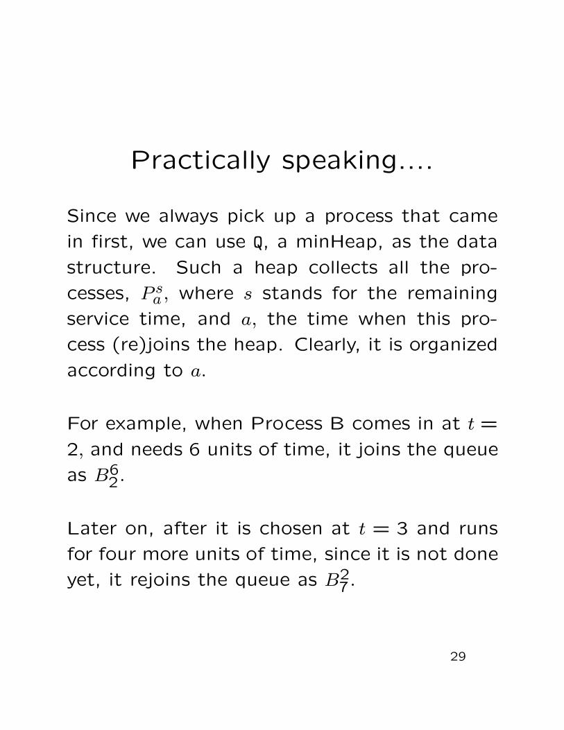
Practically speaking....

Since we always pick up a process that came

in first, we can use Q, a minHeap, as the data

structure. Such a heap collects all the pro-

cesses, P sa , where s stands for the remaining

service time, and a, the time when this pro-

cess (re)joins the heap. Clearly, it is organized

according to a.

For example, when Process B comes in at t =

2, and needs 6 units of time, it joins the queue

as B62.

Later on, after it is chosen at t = 3 and runs

for four more units of time, since it is not done

yet, it rejoins the queue as B27.

29

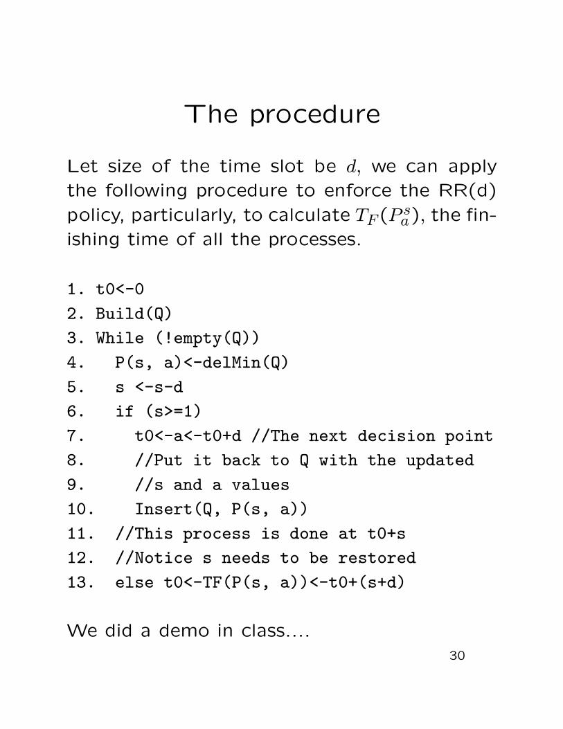
The procedure

Let size of the time slot be d, we can apply

the following procedure to enforce the RR(d)

policy, particularly, to calculate TF(P sa), the fin-

ishing time of all the processes.

1. t0<-0

2. Build(Q)

3. While (!empty(Q))

4. P(s, a)<-delMin(Q)

5. s <-s-d

6. if (s>=1)

7. t0<-a<-t0+d //The next decision point

8. //Put it back to Q with the updated

9. //s and a values

10. Insert(Q, P(s, a))

11. //This process is done at t0+s

12. //Notice s needs to be restored

13. else t0<-TF(P(s, a))<-t0+(s+d)

We did a demo in class....

30

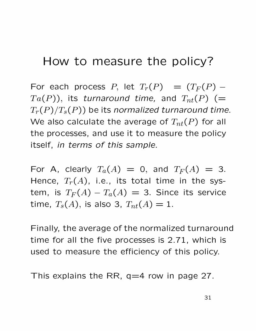
How to measure the policy?

For each process P, let Tr(P ) = (TF (P ) −

Ta(P )), its turnaround time, and Tnt(P ) (=

Tr(P )/Ts(P )) be its normalized turnaround time.

We also calculate the average of Tnt(P ) for all

the processes, and use it to measure the policy

itself, in terms of this sample.

For A, clearly Ta(A) = 0, and TF(A) = 3.

Hence, Tr(A), i.e., its total time in the sys-

tem, is TF (A) − Ta(A) = 3. Since its service

time, Ts(A), is also 3, Tnt(A) = 1.

Finally, the average of the normalized turnaround

time for all the five processes is 2.71, which is

used to measure the efficiency of this policy.

This explains the RR, q=4 row in page 27.

31

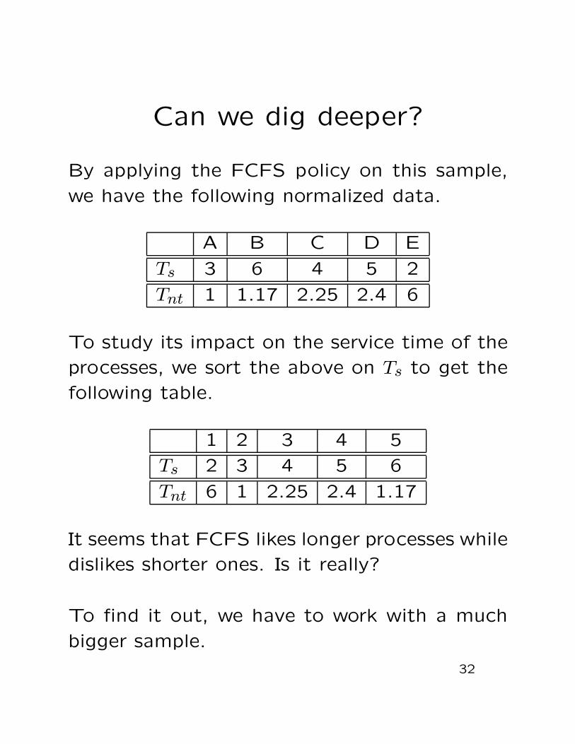
Can we dig deeper?

By applying the FCFS policy on this sample,

we have the following normalized data.

A B C D E

Ts 3 6 4 5 2

Tnt 1 1.17 2.25 2.4 6

To study its impact on the service time of the

processes, we sort the above on Ts to get the

following table.

1 2 3 4 5

Ts 2 3 4 5 6

Tnt 6 1 2.25 2.4 1.17

It seems that FCFS likes longer processes while

dislikes shorter ones. Is it really?

To find it out, we have to work with a much

bigger sample.

32

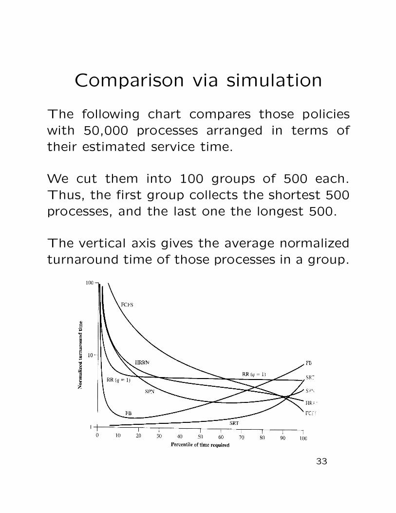
Comparison via simulation

The following chart compares those policies

with 50,000 processes arranged in terms of

their estimated service time.

We cut them into 100 groups of 500 each.

Thus, the first group collects the shortest 500

processes, and the last one the longest 500.

The vertical axis gives the average normalized

turnaround time of those processes in a group.

33

What do we find out?

FCFS is indeed pretty bad: For about a third

of the shorter processes, its turnaround time

in the system is more than 10 times of its ser-

vice time. It does come down for the longer

processes.

On the other hand, the round robin approach

is much better, except for the shortest pro-

cesses, the ratio is about 5. The SPN pol-

icy works even better, and its non-preemptive

version, the SRT definitely favors the shorter

processes.

The HRRN is supposed to be a compromise

between the FCFS and the SRT: the former

prefers the longer ones while the latter the

shorter ones, and it does work that way.

Finally, FB does work out for the shorter pro-

cesses, while the longer ones will be drifting all

the way up.

34

Fair-share scheduling

All of the scheduling algorithms we have dis-

cussed so far treat the collection of ready pro-

cesses as a single pool.

On the other hand, in a multiuser environment,

an application program, or a job, may be orga-

nized as a collection of processes. Thus, from

a user’s point of view, she will not care too

much about how a specific process is doing,

but how her processes are doing collectively.

Under a fair-share algorithm, scheduling deci-

sion will be made based on process sets, rather

than a single process.

The same concept can be further extended to

a user sets, instead of process sets. Hence, if a

large number of users log into the system, the

response time should be degenerated for that

group, and other users will not be affected.

35

More specifically,...

each user is assigned a weight that defines her

share of the system resource, including a share

for the processor. This assignment is more or

less linear, in the sense that if the share of user

A is twice as much as that of user B, then user

A should be able to do twice as much work as

user B.

The objective of such a policy is to give more

resources to users that have not used up their

fair share, and less to those that have.

36

The general policy

FSS is one implementation of such a policy.

The system classifies all users into fair share

groups, and allocates a certain percentage of

system resources to each group. It then makes

scheduling decision based on the execution his-

tory of those user groups, as well as that of

individual users.

Each process is assigned a base priority, which

drops when the process uses the processor, and

when its associated group uses the processor.

37

An example

Let’s consider an example involved with three

processes: A belongs to one group and pro-

cesses B and C belong to another group.

Each group has a weight of 0.5. When a pro-

cess is executed, it will be interrupted 60 times

a second, during which a usage field will be in-

cremented; and the priority will be recalculated

at the end of each second.

If a process is not executed, its usage will stay

the same, but its group usage goes up if any

of the processes in its group is executed.

38

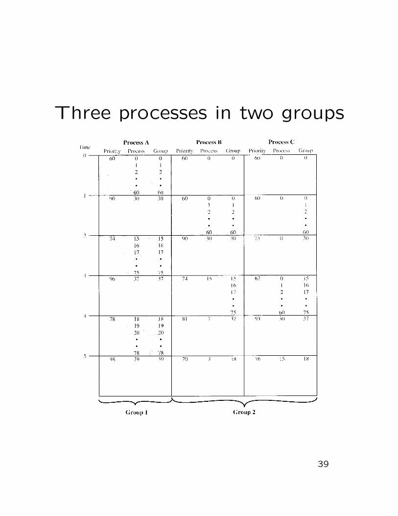
Three processes in two groups

39

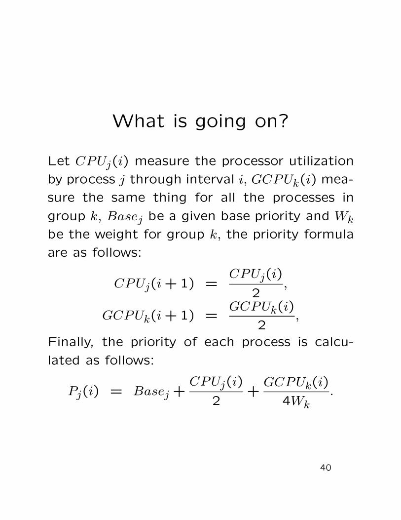
What is going on?

Let CPUj(i) measure the processor utilization

by process j through interval i, GCPUk(i) mea-

sure the same thing for all the processes in

group k, Basej be a given base priority and Wk

be the weight for group k, the priority formula

are as follows:

CPUj(i + 1) =CPUj(i)

2,

GCPUk(i + 1) =GCPUk(i)

2,

Finally, the priority of each process is calcu-

lated as follows:

Pj(i) = Basej +CPUj(i)

2+

GCPUk(i)

4Wk.

40

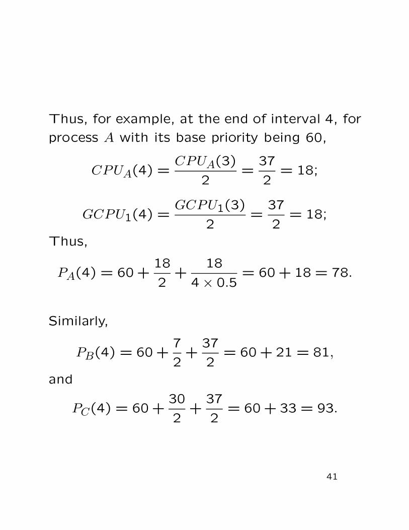
Thus, for example, at the end of interval 4, for

process A with its base priority being 60,

CPUA(4) =CPUA(3)

2=

37

2= 18;

GCPU1(4) =GCPU1(3)

2=

37

2= 18;

Thus,

PA(4) = 60 +18

2+

18

4 × 0.5= 60 + 18 = 78.

Similarly,

PB(4) = 60 +7

2+

37

2= 60 + 21 = 81,

and

PC(4) = 60 +30

2+

37

2= 60 + 33 = 93.

41

UNIX scheduling

A traditional UNIX scheduling algorithm uses

multilevel feedback using round robin in each

of its priority queues. It also uses a one-second

preemption, namely, if a process is not blocked,

or completed, within a second, it is out. Pri-

ority is assigned to each process based on its

type and execution history, and is recalculated

every second.

Processes are also put into bands of different

priority levels to optimize access to block de-

vices and allow OS to respond more quickly to

certain types of processes.

Homework: Finish off §9.3 to get into more

details of the UNIX scheduling strategies. Ex-

plain and compare what is going on in Fig-

ure 9.17 with Figure 9.16.

42