i
Western Australia School of Mines Department of Exploration Geophysics
The use of distributed sensor arrays in electrical and electromagnetic imaging
Margarita L. Norvill
This thesis is presented for the Degree of Master of Philosophy
of Curtin University
June 2011

ii

iii
This thesis is dedicated to Philippa.
Thank you for always showing an interest.

iv
Abstract ________________________________________________________________________
Electrical methods for exploring the earth, such as direct current resistivity, induced polarization
and electromagnetism are used for numerous exploration, engineering and environmental
applications. Common to all these applications is the desire to obtain the clearest possible image of
the target. This thesis analyses and develops methods for improving signal to noise ratio for
electrical methods.
The ability to recover subsurface information from electrical exploration methods is dependent on
the limits of signal detection which is strongly influenced by instrumentation and the conductivity
structure of the Earth. Multiple sensors can be used to collect data efficiently over a survey area.
Such multi-receiver arrays can improve the signal-to-noise ratio. However, the use of multiple
sensors can also be exploited to improve the signal fidelity from each sensor, which may then
translate to more accurate geological models and/or greater depth of investigation. In this thesis a
two step algorithm for the removal of harmonic noise and atmospheric transients is presented. The
first step is the removal of harmonic noise from each sensor using a non-linear single value
decomposition (SVD) inversion technique to model a modulated sinusoid to narrow band noise
sources. The second step is spherics attenuation using an iterative technique of signal stripping then
removing residual coherent noise across the array combined with robust statistical measures in the
stacking process. I show that this approach can recover signals otherwise buried in noise and that
under certain conditions, signal to noise ratio can be improved by more than 46 dB. The algorithms
designed here are applicable to any type of electrical or time domain electromagnetic survey
conducted with a multi-receiver array.

v
Acknowledgments ________________________________________________________________________
Thanks to the staff and students of the Curtin University Exploration Geophysics
Department for all their support and friendship, particularly Anton Kepic, Norm Uren,
Bruce Hartley, Dominic Howman, Jayson Meyers, Deirdre Hollingsworth, Don Hunter,
Mohammed Rosid, Kirtsy Beckett, Julianna Toms and Justin Vermeulen.
I am grateful to Bill Amann, Terry Ritchie and Jock Buselli for their technical advice and
provision of data sets.
Thanks to APA-I and CRC LEME for financial assistance.
I am appreciative of all the support from my friends and family: Sue Norvill, Bruce Thorpe,
Elsa Murray, Elise Steckis, Hayden Still, Shelley Leaver, Philippa Schrape, Amber Vigilo
and to Bruno Kongawoin for his encouragement and support at the end.
vi
Contents ________________________________________________________________________
Abstract iv
Acknowledgments v
Contents vi
List of Figures vii
1. Introduction 1
2. Noise Characteristics 4
2.1. Observation Noise Characteristics 8
2.2. Time Dependent EM Noise 10
2.3. Spherics Characteristics 14
2.3.1. Synthetic Spherics 17
2.4. Cultural Noise Characteristics 21
2.4.1. Synthetic Modulated Powerline Harmonics 24
3. Signal Processing 27
3.1. Pre-Whitening and Deconvolution 27
3.2. Stacking 32
3.3. Robust Statistics 36
4. Powerline Harmonics 41
4.1. Inversion 42
4.1.1. Non-linear SVD Inversion for Modulated Harmonics 43
5. Array Processing 49
6. Conclusion and Recommendations 58
References 60
Appendix 1. Data Acquisition 65
1A. MIMDAS IP 65
1B. IP Survey at Curtin University 66
1C. EM Survey at Curtin University 66
1D. Noise recording in Darwin 67

vii
List of Figures ________________________________________________________________________
Figure 2.1. A synthetic time domain EM transmitted waveform. 6 Figure 2.2. Amplitude spectrum of a synthetic time domain EM transmitted 7 waveform in the frequency domain. Figure 2.3. Generalized geomagnetic spectrum for horizontal magnetic 11
field (H) and induced voltage (V) measurements reproduced from Spies and Frischknecht, 1991.
Figure 2.4. Spherics activity recorded in Darwin, the summer of 1983, data 15 Courtesy of J. Buselli, CSIRO.
Figure 2.5. Amplitude spectrum of spherics activity recorded in Darwin 16 summer of 1983, data courtesy of J. Buselli, CSIRO.
Figure 2.6. Spheric event recorded in Darwin, the summer of 1983, data 19 courtesy of J. Buselli, CSIRO.
Figure 2.7. Unconstrained non-linear optimization to fit real spherics. 20 Figure 2.8. IP survey at Curtin University showing modulated harmonics. 22 Figure 2.9. MIMDAS IP data showing modulated harmonics and weak 23 non-stationary components, data courtesy of T. Ritchie,
Xstrata Pty Ltd. Figure 2.10. Synthetic data showing modulated harmonics. 25 Figure 2.11. Amplitude spectrum of synthetic data showing modulated 26
harmonics. Figure 3.1. Synthetic spherics. 29 Figure 3.2. Spiking deconvolution operator derived from spheric events. 30 Figure 3.3. Convolution of spiking deconvolution operator with spheric. 31 Figure 3.4. Stacking for a robust estimate of the received signal. 35 Figure 3.5. Signal rectification. 37 Figure 3.6. Stacking prior to robust statistics and iterative stacking. 38 Figure 3.7. Robust statistics as a means of removing low frequency noise. 39 Figure 3.8. Robust statistics as a means of removing high frequency noise. 40 Figure 4.1. Harmonic noise removal; the initial estimate the harmonic 46 frequency, stage one. Figure 4.2. Harmonic noise removal; the initial estimate the harmonic 47 frequency, stage two. Figure 4.3. Comparison of the received signal before and after powerline 48 harmonic attenuation. Figure 5.1. Array processing flow chart. 54 Figure 5.2. Array processing a field example: Curtin electrical data array 55 processing.

viii
List of Figures ________________________________________________________________________
Figure 5.3. Array processing a field example: Curtin electromagnetic 56 data array processing. Figure 5.4. Array processing a field example: MIMDAS data array processing, 57 data courtesy of T. Ritchie, Xstrata Pty Ltd.

1
1. Introduction ________________________________________________________________________
Electrical methods for exploring the earth, such as direct current resistivity, induced
polarisation (IP) and electromagnetism are used for numerous exploration, engineering and
environmental applications. Common to all applications is the desire to obtain the clearest
image of the target signal as possible.
In mineral exploration there is a continuing pursuit of both new ore bodies, and more
precise 3D imaging of existing ore bodies. Since the shallow targets have mostly been
discovered, the minerals industry is increasingly focused on deeper targets.
Electromagnetic exploration methods need to be improved to maintain acceptable
resolution for deeper targets. One way to achieve this is to improve signal to noise ratio at
the EM receivers. Our ability to measure rapidly changing small EM fields in and above the
earth is impeded by the presence of natural and cultural electromagnetic noise. Improved
acquisition and processing for the electromagnetic methods are required if greater depth of
penetration for the technique is to be achieved.
Environmental and engineering electromagnetic surveys are often carried out in proximity
of industrial and residential areas. The electromagnetic noise in these areas is more
complex as it originates from many different sources such as inductive load imbalances and
switching transients. These noise sources are termed “cultural” as they relate with activity
of mankind and are different from the “natural” noise sources which relate to natural Earth
processes and solar activity. The important difference between these two sources of noise is
their level of coherency over short periods of time. Given the inertia of the electrical grid,
cultural noise tends to be more or less stationary and coherent for periods under one second.
Natural noise sources are more or less stochastic events. Fortunately, the short-term
coherency of cultural noise allows it to be estimated, then subtracted from data records.
This approach is explored in details in the following chapters.

2
The complexity of the new targets have caused a resurgence in; (i) the use of multi-
electrode receiver systems in DC electrical resistivity, (ii) IP methods (e.g. White et al.,
2001) and (iii) the use of multiple receiver systems for the time-domain electromagnetic
method. This increase in the number of receivers offers the potential for deeper
penetration, improved resolution, and detection of weak conductors. These benefits can be
extracted from richer multi-receiver datasets with the help of signal processing algorithms
that use the additional information to improve the target response. A major objective of this
thesis is to design and test a multichannel processing algorithms designed to improve the
data measured from arrays of time domain EM receivers.
To assist the reader, this thesis has been divided into five chapters. Chapter two examines
noise sources that can contaminate electrical data and their impact on the quality of the
electrical data that can be recorded. This chapter also introduces algorithms designed to
generate synthetic noise series to be used for testing of the noise suppression algorithms
developed in Chapters 3, 4 and 5.
Chapter three provides a review of traditional signal processing methods for time domain
electromagnetic and electrical methods. Also I introduce the possible use of spiking
deconvolution as a tool for spherics elimination. This chapter concludes with a novel
approach to stacking and the use of robust statistics.
Chapter Four investigates inversion methods for the removal of powerline harmonics. In
this chapter I introduce an innovative approach of single value decomposition (SVD)
inversion for the removal of modulated powerline harmonics.
Chapter Five reviews remote reference techniques for noise minimization, and presents a
two step array processing algorithm for the removal of harmonic noise and atmospheric
transients. The first step is the removal of harmonic noise from each sensor using the non-
linear SVD inversion technique presented in Chapter Four. The second step is spherics
attenuation using an iterative technique of signal stripping then removing residual coherent

3
noise across the array. This is combined with robust statistical measures in the stacking
process.
4
2. Noise Characteristics ________________________________________________________________________
The objective of a geophysical survey is to obtain information about the spatial distribution
of one or more of the Earth’s physical properties from a limited set of measurements of a
related physical field. The electrical properties of the subsurface may be determined using
either static or time varying electromagnetic fields (CSEM). Methods that rely on static
fields rely on a steady flow of current in the ground. Controlled source electromagnetic
methods, on the other hand, rely on the propagation of electromagnetic fields from a time
varying electric or magnetic source (West and Macnae, 1991; Parasnis, 1997). Signal to
noise ratio is fundamentally important when measuring late time responses from conductive
targets. Variations in the received signal due to the target must be observable in the
presence of natural and cultural noise sources. The received signal is composed of the
actual target signal, time dependent EM noise, geological noise and observation noise. The
statistical properties of these three forms of noise are different, and relevant suppression
techniques are required.
This chapter considers sources of time dependent EM noise and observation noise. It also
provides a detailed review of the intrinsic noise of the receiver (observation noise), spherics
and modulated harmonics (time dependent EM noise).
For the purpose of testing processing algorithms with a controlled data set, synthetic
received waveforms are generated and imprinted with synthetic noise. The advantage of
using a synthetic receiver and noise sources is that the exact noise contributions are known,
as well as allowing for specific noise situations to be tested.
The transmitted and received signal for a DC resistivity, IP or time domain EM surveys is
essentially an alternating current (AC) or time-varying waveform. Such
alternating/changing waveforms are imperative as they allow for the influence of static
errors, instrumental drift and electronic, low frequency noise in the first amplification
stages to be removed (Becker and Cheng, 1987).

5
In this research, only the full digitized waveform is recorded, as this provides an
uninterrupted record of any noise sources as well as providing detail about the transmitter.
This leads to a better understanding of the signal and noise behavior as there is no
ambiguity over signal at any time, which leads to improved interpretation.
For the purpose of testing processing algorithms with a controlled data set, synthetic
transmitted and received waveforms can be generated for DC/IP and time domain EM data
sets. The synthetic transmitted waveform for DC/IP and time domain EM can be
approximated by a 50% duty cycle waveform with period T , having an exponential rise
with time constant τ/t , where τ is a time constant determined by the transmitter
impedance (size, resistance, Earth resistivity), and the transmitter design with duration
4/T . The turnoff ramp can be approximated as linear with a duration from 0.03 to 0.6 τ .
The last half period of the waveform is the inverse of the first half (Asten, 1987).
For time domain EM, the received waveform (for a confined conductor) is the derivative of
the transmitted waveform convolved with the Earth’s exponential response:
))exp(1(1)( ettresponseEarth τ−−−= , (2.1)
where eτ is the time constant for the Earth’s decay (Asten, 1987). Figures 2.1 and 2.2
show synthetic transmitted and received waveforms for time domain EM using equation
(2.1) in the time and frequency domain respectively.
For a layered Earth the late time Z-component response may be represented as power law
decay xt − , with x equal to 2.5 for a homogenous Earth, 4 for a conducting layer over a
resistive half space and 1 for a resistive layer over a conducting half space (Lee and
Lewis, 1974; Kaufman and Keller, 1983).

6
Figure 2.1. A synthetic time domain EM transmitted square waveform. Duty cycle 50 %, base frequency 4.166 Hz, input current 1 A current, sampling frequency 10 kHz. The received waveform is the derivative of the transmitted waveform convolved with the Earth’s response (assuming a confined conductor), Equation (2.1).

7
Figure 2.2. Amplitude spectrum of a synthetic time-domain EM transmitted waveform in the frequency domain (assuming a confined conductor). Duty cycle 50 %, base frequency 4.166 Hz, input current 1 A current, sampling frequency 10 kHz. Peaks in the amplitude spectrum occur at twice the base frequency.

8
2.1. Observation Noise Characteristics
Observation noise may be generated by the motion of the survey sensor in the Earth’s
magnetic field, the intrinsic electronic noise of the sensor, and the receiving systems
hardware and data sampling software. Motion induced noise can be a large problem, as
spurious signals can be induced in magnetic sensors by even slight movement of the sensor
in the Earth’s magnetic field. The Earth’s field is approximately hundreds of thousands
times larger than the typical fields measured in EM sounding. Therefore vibration induced
by wind can often cause appreciable noise voltages known as wind noise or microphonics
(Macnae et al., 1984; Spies and Frischknecht, 1991).
In electronic circuits, total noise free performance is impossible to achieve as noise is a
consequence of molecular motion. Intrinsic noise within the electronic components of a
circuit include:
1. White noise: random energy containing all frequencies in equal proportions within
the bandwidth, with random phases (Sheriff, 1999),
2. Pink noise: dominated by low frequencies, pink noise has the same distribution of
power for each octave, with energy equal to 1/f
3. Burst noise: noise switches between two or more discrete values at random time.
White noise is present in all resistors and semiconductors. Such noise results from the
random thermal energy of electron conduction. The average power in a given bandwidth
depends on temperature (Smith and Sheingold, 1969). Pink noise results from flicker or 1/f
noise. Semiconductors exhibit pink noise due to random fluctuations in the number of
surface re-combinations (Ryan and Scranton, 1984). Burst-noise, also known as popcorn
noise, only occurs in poorly manufactured semiconductors. It is due to random on/off
recombination action in the semiconductor material, leading to erratic switching of an
affected device’s current gain (Ryan and Scranton, 1984).

9
Most commonly the intrinsic noise of a time domain EM sensor is white noise.
Synthetically this can be represented by generating an array of Gaussian distributed random
numbers, normally distributed with a mean of zero.

10
2.2. Time Dependent EM Noise
Time-dependent EM noise is characterised by differences observed in recordings made at
the same receiver station at different times. This type of noise comprises of spherics, noise
of geomagnetic and ionospheric origin and cultural noise. Figure 2.3 shows a typical
spectral plot for geomagnetic variations averaged over a long time. Geomagnetic noise is
one of the major sources of noise in EM soundings. Below 6 Hz, the natural EM noise
field is primarily geomagnetic and of ionospheric origin. Below 1 Hz, the signal arises
mainly from within and outside the ionosphere as a result of complex interactions between
plasma emitted from the Sun with the Earth’s permanent magnetic field, known collectively
as ultra low frequency (ULF) waves (previously known as micropulsations or magnetic
pulsations). Oscillations with quasi-sinusoidal waveform are called pulsations continuous
(Pc). The waveforms that are more irregular are called pulsations irregular (Pi). Each type
is subdivided into frequency bands roughly corresponding to distinct phenomena
(McPherron, 2002). Below 0.1 Hz, the amplitude of these signals is approximately
inversely proportional to frequency (Figure 2.3). These signals are stronger during the
morning and are also stronger in equatorial regions, so they are clearly related to the
attitude of the sun. Over the range of 0.1 to 1 Hz, the steep fall off in the amplitude
spectrum is caused by attenuation of the EM fields passing through the ionosphere, which
is conductive over a broad range of frequencies (Spies and Frischknecht, 1991; San Filipo
and Hohmann, 1983). ULF waves are relatively unimportant in EM soundings, except at
very low frequencies. They can be an annoyance in IP surveys particularly Pc1 (Ritchie,
2003, pers. comm), which has period from 0.2 to 5 s (McPherron, 2002).

11
Figure 2.3. Generalized geomagnetic spectrum for horizontal magnetic field (H) and induced voltage (V) measurements reproduced from Spies and Frischknecht, 1991.

12
The main source of geomagnetic noise in the frequency range above 1 Hz is atmospheric
lightning discharges around the Earth, referred to as spherics (Figure 2.3; Spies and
Frischknecht, 1991). Spherics are impulsive events that occur over a broad range of
frequencies, and they will be discussed in greater detail in Section 2.3. The extremely low
frequency (ELF) components of spherics travel around the Earth’s ionospheric cavity and
interfere constructively and destructively, resonating at 8, 14, 20, 26 and 32 Hz, the
Schumann resonances. The ionosphere has strong absorption between 500 Hz and 2.3 kHz,
resulting in a low spectral density of geomagnetic noise in this region (Macnae et al., 1984;
Spies and Frischknecht, 1991).
Cultural noise arises mainly from power distribution grids. Depending on the country, the
mains frequency has its fundamental at either 50 or 60 Hz but higher order harmonics can
prove as equally damaging within the measured time series. While the United States,
Canada Japan and parts of South America opted to run their power grids at 60 Hz, the
majority of the world opted to run them at 50 Hz. This difference arose from the different
types of generators developed during the introduction of electricity. In developed countries,
the inertia of the power grid is very substantial and thus the frequency drift of the
fundamental frequency is limited to less than 2% of its nominal value. In areas where the
power grid is less developed and has minimal power factor correction, the fundamental
frequency observed on the grid can vary up to 10 % of its nominal value (Macnae et
al., 1984; Spies and Frischknecht, 1991; Zonge and Hughes, 1991). Such cultural noise
will be discussed in details in Section 2.4.
Communication signals are another major source of noise which occupy the higher portion
of the electromagnetic spectra. The Navy uses Very Low Frequency (VLF) communication
transmissions that produce strong signals in the range of 15 to 24 kHz (McNeill and
Labson, 1991). The advent of global positioning systems (GPS) brought an end to military
positioning signals such as the United States OMEGA VLF communications, and thus they
are no longer a noise source but it remains important to be aware of these signals when
processing older data sets. Radio and radar stations broadcast at much higher frequencies,

13
but may often overload induction EM systems that do not incorporate sufficient filtering
and shielding. They may also preclude the possibility of making soundings (Spies and
Frischknecht, 1991).
14
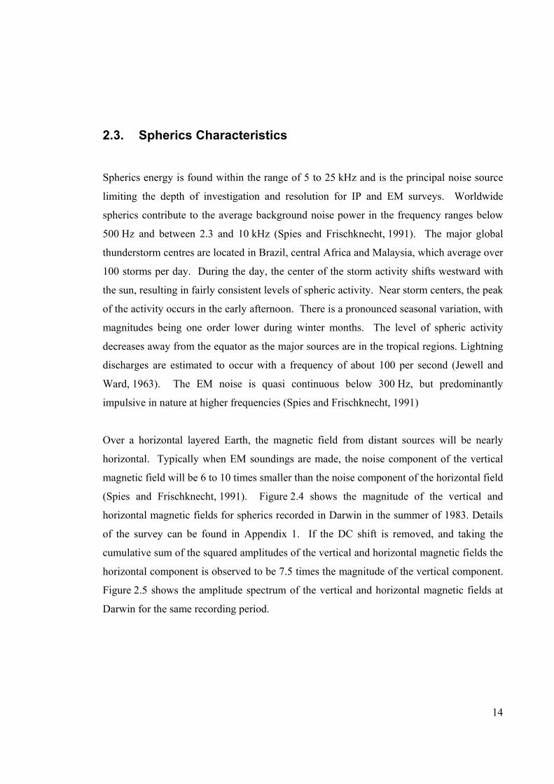
2.3. Spherics Characteristics
Spherics energy is found within the range of 5 to 25 kHz and is the principal noise source
limiting the depth of investigation and resolution for IP and EM surveys. Worldwide
spherics contribute to the average background noise power in the frequency ranges below
500 Hz and between 2.3 and 10 kHz (Spies and Frischknecht, 1991). The major global
thunderstorm centres are located in Brazil, central Africa and Malaysia, which average over
100 storms per day. During the day, the center of the storm activity shifts westward with
the sun, resulting in fairly consistent levels of spheric activity. Near storm centers, the peak
of the activity occurs in the early afternoon. There is a pronounced seasonal variation, with
magnitudes being one order lower during winter months. The level of spheric activity
decreases away from the equator as the major sources are in the tropical regions. Lightning
discharges are estimated to occur with a frequency of about 100 per second (Jewell and
Ward, 1963). The EM noise is quasi continuous below 300 Hz, but predominantly
impulsive in nature at higher frequencies (Spies and Frischknecht, 1991)
Over a horizontal layered Earth, the magnetic field from distant sources will be nearly
horizontal. Typically when EM soundings are made, the noise component of the vertical
magnetic field will be 6 to 10 times smaller than the noise component of the horizontal field
(Spies and Frischknecht, 1991). Figure 2.4 shows the magnitude of the vertical and
horizontal magnetic fields for spherics recorded in Darwin in the summer of 1983. Details
of the survey can be found in Appendix 1. If the DC shift is removed, and taking the
cumulative sum of the squared amplitudes of the vertical and horizontal magnetic fields the
horizontal component is observed to be 7.5 times the magnitude of the vertical component.
Figure 2.5 shows the amplitude spectrum of the vertical and horizontal magnetic fields at
Darwin for the same recording period.

15
Figure 2.4. Spherics activity recorded in Darwin, the summer of 1983, data courtesy of J. Buselli, CSIRO. (a) Vertical component of magnetic field showing spherics. (b) Horizontal component of magnetic field showing spherics. Notice the impulsive nature of spherics. The magnitude of the horizontal component of the magnetic field is 7.5 times the vertical component. Details of this data recording are in Appendix 1.

16
Figure 2.5. Amplitude spectrum of spherics activity recorded in Darwin summer of 1983, data courtesy of J. Buselli, CSIRO. (a) Amplitude spectrum of the vertical component of magnetic field showing spherics. (b) Amplitude spectrum of the horizontal component of magnetic field showing spherics. The spectrum indicates that the storm activity was nearby as the high frequency components are dominant and have not been absorbed. These plots also show the broadband nature of spherics as a noise source. Details of this data recording are in Appendix 1.

17
2.3.1. Synthetic Spherics
A heuristic approach was taken to generating synthetic spherics. Figure 2.6 shows an
example of a spheric event recorded in Darwin in the summer of 1983. Details of the data
recording are in Appendix 1. A lightning strike can generally be described as being a
minimum phase impulse response. A minimum phase signal has the energy concentrated at
the onset. When there are multiple global sources and spheric events, the minimum phase
assumption may no longer hold as the signals can merge. Very strong transients usually
come from nearby or intermediate distances < 1000 km. Figure 2.6 (b) shows that the
spheric response is comprised of a multitude of frequencies. In this case the dominant
frequencies are centered at 5 kHz and 8.5 kHz. I theorized that a spheric event can be
approximated by exponentially damped sinusoids as:
+
++
++
+
= G
tFE
tDC
tB
tA
tSph
5sin
5sin
5sin
5exp
5
4
++
++
+
+
Pt
ONt
MLt
KJt
It
H5
sin5
sin5
sin5
exp5
3
. (2.2)
Using Equation (2.2) and field data recorded at Darwin, the constants A through P were
solved using a Matlab Mathworks Inc. function file for unconstrained, non-linear
optimisation. Figure 2.7 shows the original spheric events and the modeled spheric events
using Equation (2.2).
Equation (2.2) can then be simplified to:
+
= CR
tBR
tA
tSph ***
4
5sin
5exp
5
+
+
+ LR
tKRJR
tI
tH *****
3
5sin
5exp
5, (2.3)

18
where *R is a random number between zero and one, with uniform distribution;
**R is a
random number, normally distributed with a mean of zero, variance one and standard
deviation one; and A through G are constants used to define the spheric response.

19
Figure 2.6. Spheric event recorded in Darwin, the summer of 1983, data courtesy of J Buselli, CSIRO. (a) Vertical component of magnetic field. (b) The amplitude spectrum of the spheric event. The time series data show the impulsive nature of spherics. The amplitude spectrum indicates the frequency of the spheric event is concentrated at around 5 kHz and 8.5 kHz. Details of this data recording are in Appendix 1.

20
Figure 2.7. Unconstrained non-linear optimisation to fit real spherics. Example of two spherics captured from the Darwin vertical component data with fit for Equation (2.2). Data courtesy of J. Buselli, CSIRO.

21
2.4. Cultural Noise Characteristics
The powerline voltage waveform is generally sinusoidal. However, the current waveform
is often complicated. Motor loads operate non-synchronously and produce more damaging,
but weaker non-stationary components, such as switching transients, sidebands and sub-
harmonics. The simple switching of current loads and the electronic cycle by cycle
switching of rectifiers in many power systems produce broadband transients and high
frequency harmonics. Electric rail roads in Europe are often a source of large amplitude,
13 2/3 Hz noise (Macnae et al., 1984; Spies and Frischknecht, 1991; Zonge and Hughes,
1991). In surveys located at mine sites, the Person Emergency Device (PED) may
contaminate the received signal. PED transmissions occur over the range of 362 to 386 Hz.
PED signals are not sinusoidal, and thus have some power at higher harmonics; notably the
3rd, 5th and 2nd (Duncan, 2002).
Generally the powerline EM field consists of a series of Dirac-delta functions at the mains
frequency and its harmonics, then a multitude of much weaker and more contaminating
non-stationary components, Figures 2.8 and 2.9 show examples of data contaminated with
harmonic noise. Figure 2.8 is an example of data collected in an urban environment
(electrical data collected at Curtin University, details in section Appendix 1) and Figure 2.9
is an exploration example (IP data collected with Mount Isa Mines’ distributed acquisition
system (MIMDAS), details in section Appendix 1). Where powerline harmonics are
modulated, the time series shows a variation in amplitude, known as the modulation
envelope, seen in Figure 2.8 and 2.9. The amplitude spectrum modulation is indicated by
multiple spikes instead of clear spectral lines, Figure 2.8 and 2.9.

22
Figure 2.8. IP survey at Curtin University showing modulated harmonics. (a) Section of time series. (b) The amplitude spectrum of IP survey. The time series shows varying overall amplitude, indicating harmonic modulation. Peaks in the amplitude spectrum at 3.4 and 9.65 Hz are due to the received signal occurring at increments of the base frequency 3.125 Hz. The peak at 50 Hz is due to the powerline harmonics. Details of this data recording are in section Appendix 1.

23
Figure 2.9. MIMDAS IP data showing modulated harmonics and weak non-stationary components, data courtesy of T. Ritchie, Xstrata Pty Ltd. (a) Section of time series. (b) Sections of the amplitude spectrum. Peaks in the amplitude spectrum for the IP received waveform occur at twice the base frequency of 0.0997 Hz. The peak at 50 Hz is due to powerline harmonics. Peaks in the amplitude spectrum at 14.8, 15, 18.3 and 18.5 Hz are due to weak non-stationary components. There are multiple peaks at 14.8 Hz and 50 Hz, indicating modulation. Details of this data recording are in section Appendix 1.

24
2.4.1. Synthetic Modulated Powerline Harmonics
A heuristic approach was taken to generating synthetic amplitude modulated powerline
harmonics. A stationary sinusoid can be represented by:
( ) ( ) ( )=
+=n
i
iiii tfbtfatmS1
2cos2sin, ππ, (2.4)
where if is the frequency of the sinusoid, t is time, ia and ib are the amplitudes of the
sine and cosine components (the ratio of these is directly related to the phase of the
sinusoid), and n is the number of sinusoid functions needed to model the sinusoidal noise.
Harmonic noise with amplitude modulation can be represented as a summation of sinusoids
with a sinusoidal function defining the modulation envelope with the harmonic component
at a single sensor, it can be then be given as;
( ) ( ) ( ) ( ) ( )=
+=n
iiiiiii tfthbtfthatmS
1
2cos2sin2sin2sin, ππππ, (2.5)
where ih is the frequency of the modulation envelope. Figures 2.10 and 2.11 show
modulated harmonics produced by Equation (2.5)

25
Figure 2.10. Synthetic data showing modulated harmonics. (a) Synthetic modulated harmonics generated using Equation 2.5 (b) Synthetic modulated harmonics with synthetic a time domain EM waveform, generated using equation 2.1 and 2.5. The time series show varying amplitude, indicating harmonic modulation.

26
Figure 2.11. Amplitude spectrum of synthetic data showing modulated harmonics. (a) Synthetic modulated harmonics generated using equation 2.5(b) Synthetic modulated harmonics with synthetic time domain EM waveform, generated using equation 2.1 and 2.5. Peaks in the amplitude spectrum at 50, 100, 150, 200, 300 350 and 400 Hz due to the powerline harmonics.

27
3. Signal Processing ________________________________________________________________________
There has been comprehensive research into noise sources and noise reduction techniques
for electrical methods used in geophysics. Chapter two reviewed the characteristics of
observation noise and time dependent EM noise, primarily spherics and powerline
harmonics. At present, a number of data processing steps can be preformed on the data, to
improve the signal to noise (S/N) in the presence of these noise sources:
1) Stacking (averaging) the signal over time and increasing the transmitted field. The
target signals increase linearly with the magnitude of the inducing field and is phase
coherent with it. Therefore, relative noise amplitude is decreased by both averaging in
time and increasing the transmitted field. Instrument averaging or stacking rejects
random, events such as electronic noise and distant spheric activity.
2) Pruning (data rejection) of non-stationary intense transients, such as local spherics or
powerline transients.
3) Modification to weighting of a stack to improve the rejection of line spectrum noise.
4) Signal modification by pre-emphasis/de-emphasis to accommodate the non-white
character of the spheric noise spectrum.
These steps are discussed in greater detail in Buselli and Cameron, 1996; Macnae et al.,
1984; and McCracken et al., 1986b.
3.1. Pre-whitening and Deconvolution
Natural EM noise originates mainly from spherics. Spherics energy is not uniformly
distributed through the system bandwidth. It is concentrated at the high frequency end of a
typical EM system bandwidth (Figure 2.5). It is possible to redistribute the power in the
transmitted spectrum and compensate in the receiver by filtering the signal and noise. Such
techniques are known as pre-emphasis pre-whitening and deconvolution. The main
obstacle to their use in EM is the necessary preservation of phase characteristics in filters
(Macnae et al., 1984). When applying a filter to the transmitter current, with a realisable
28
inverse, if the inverse filter is applied to the received signal, the earth response will be the
same while the noise is filtered via the inverse filter. Optimisation (or pre-emphasis) is a
complex process for any EM system, as the noise spectrum is far from constant and the
process is limited by the achievable voltage and current limits of the transmitter.
Optimisation can be formalised and the conditions for this are that the noise spectrum is
known and constant, the relative precision on different channels is stated, and the norm of
the transmitter is fixed (Macnae et al., 1984 and Duncan, 2002).
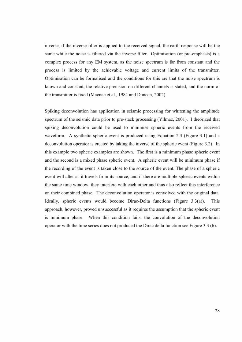
Spiking deconvolution has application in seismic processing for whitening the amplitude
spectrum of the seismic data prior to pre-stack processing (Yilmaz, 2001). I theorized that
spiking deconvolution could be used to minimise spheric events from the received
waveform. A synthetic spheric event is produced using Equation 2.3 (Figure 3.1) and a
deconvolution operator is created by taking the inverse of the spheric event (Figure 3.2). In
this example two spheric examples are shown. The first is a minimum phase spheric event
and the second is a mixed phase spheric event. A spheric event will be minimum phase if
the recording of the event is taken close to the source of the event. The phase of a spheric
event will alter as it travels from its source, and if there are multiple spheric events within
the same time window, they interfere with each other and thus also reflect this interference
on their combined phase. The deconvolution operator is convolved with the original data.
Ideally, spheric events would become Dirac-Delta functions (Figure 3.3(a)). This
approach, however, proved unsuccessful as it requires the assumption that the spheric event
is minimum phase. When this condition fails, the convolution of the deconvolution
operator with the time series does not produced the Dirac delta function see Figure 3.3 (b).

29
Figure 3.1. Synthetic spherics (a) Minimum phase spheric event (b) Mixed phase spheric event (c) Amplitude spectrum of minimum phase spheric event (d) Amplitude spectrum of mixed phase spheric event. The two synthetic spheric events have similar amplitude spectrums and though their phase spectra differ. The phase spectrum controls the shape of the waveform.

30
Figure 3.2. Spiking deconvolution operator derived from spheric events. (a) Operator derived using a minimum phase spheric event (b) and its amplitude spectrum (c) Operator derived using a mixed phase spheric event and its amplitude spectrum (d).

31
Figure 3.3 Convolution of spiking deconvolution operator with spheric. The desired output is the Dirac delta function (a) when using a mixed phase spheric to derive the deconvolution operator the operation fails (b). The desired output is a flat amplitude spectrum (c) the effect of the spheric has not been removed from (d).

32
3.2. Stacking
Stacking is the collective binning of a geophysical measurement in one location. The
number of stacks is chosen to provide a balance between available time for acquisition,
available computer memory (in the case of full waveform measurements) and the number
of necessary measurements to produce repeatable measurements. In most cases, data are
stacked by the instrument during recording using a boxcar integrator type approach.
However, the boxcar integrator is essentially a single channel device and the detection of
geophysical signals is generally done with a number of gates activated sequentially, usually
with six to fifty channels. Gate widths and positions are set to fully recover the expected
signal (Becker and Cheng, 1987). Data are gated by averaging groups of adjacent samples.
The data groups are coherently sorted into channels with each channel containing a subset
of the acquired data. The acquisition is synchronised with the transmitter so the delay
between the commencement of the signal cycle and the positioning of the data group is
constant. The sorting (or windowing) process is followed by rectification, consistent with
the signal polarity changes and averaging of the rectified data. Usually these two processes
are combined into a single digital filtering operation (Becker and Cheng, 1987). In the case
of electronic rectification it is difficult to achieve exact equality in processing the plus and
minus half cycles. The resulting bias may be eliminated by interchanging processing paths
in the receiver at regular intervals during stacking. The output is then a sum of several
smaller stacks, rather than one continuous stack. This procedure has no effect on the
spectral sensitivity for uncorrelated noise (Macnae et al., 1984).
Field data normalised with respect to the transmitter current or calculated primary field and
receiver coil moment. In certain cases, the finite transmitter turn off is also corrected
(Nabighian and Macnae, 1991). For certain types of non-stationary noise, such as spherics
or coherent noise caused by powerlines, it is possible to increase S/N ratios above those
obtained by simple stacking for an equal time by use of techniques such as tapered
stacking, randomised stacking or pruning (data rejection) of non-stationary intense
33
transients, such as local spherics or powerline transients (Macnae et al., 1984; Spies and
Frischknecht, 1991; Nabighian and Macnae, 1991).
Tapered stacking, which is the convolution of the received signal with a tapered window,
will increase the central acceptance peak and reduce the side lobe amplitude in comparison
to a rectangular filter in the frequency domain (Macnae et al., 1984). If noise is white,
simple stacking will result in a better S/N ratio than tapered stacking. However reduction
of side lobes may be favourable if strong monochromatic noise is present (Macnae et al.,
1984). Powerline noise, high frequency VLF interference and any other narrow bandwidth,
coherent interference, is removed far more effectively with tapered stacking. Powerline
filtering will improve at higher base frequencies (Duncan, 2002).
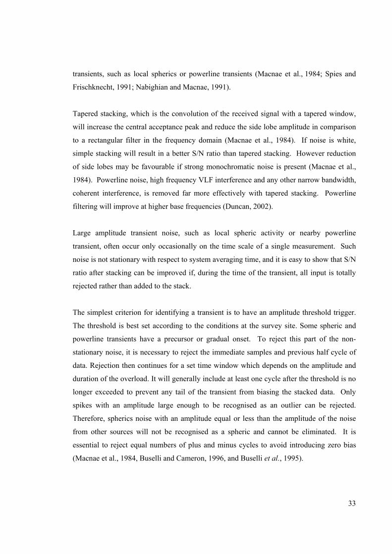
Large amplitude transient noise, such as local spheric activity or nearby powerline
transient, often occur only occasionally on the time scale of a single measurement. Such
noise is not stationary with respect to system averaging time, and it is easy to show that S/N
ratio after stacking can be improved if, during the time of the transient, all input is totally
rejected rather than added to the stack.
The simplest criterion for identifying a transient is to have an amplitude threshold trigger.
The threshold is best set according to the conditions at the survey site. Some spheric and
powerline transients have a precursor or gradual onset. To reject this part of the non-
stationary noise, it is necessary to reject the immediate samples and previous half cycle of
data. Rejection then continues for a set time window which depends on the amplitude and
duration of the overload. It will generally include at least one cycle after the threshold is no
longer exceeded to prevent any tail of the transient from biasing the stacked data. Only
spikes with an amplitude large enough to be recognised as an outlier can be rejected.
Therefore, spherics noise with an amplitude equal or less than the amplitude of the noise
from other sources will not be recognised as a spheric and cannot be eliminated. It is
essential to reject equal numbers of plus and minus cycles to avoid introducing zero bias
(Macnae et al., 1984, Buselli and Cameron, 1996, and Buselli et al., 1995).

34
McCracken et al. (1984) state it is possible to remove a spheric from the data stream and
replace it with synthetic data, rather than nulling the time-series. This introduces less noise
into the stacked data. Where both strong transients and narrowband noise are present,
taking random stacks improves the data fidelity, except for noise at odd harmonics of the
base frequency. To avoid zero bias and sensitivity to the even harmonics of the transmitter
base frequency, it is necessary that equal numbers of plus and minus cycles to be stacked
(Macnae et al., 1984). It is possible to apply both pruning and tapered stacking to the same
data set, but because pruning is a step function, it reintroduces the power side lobes that
tapered averaging is designed to remove, and may also lead to bias in the output (Macnae et
al., 1984).
Iterative stacking in conjunction with single value decomposition (SVD) inversion for
harmonic removal (Section 4.1.1) and robust statistics for attenuation of observation noise
was the most effective. This will be explored in detail in Section 3.3 on robust statistics
and in the array processing chapter (Chapter 5).
A method is reviewed where stacking was used to get a robust estimate of the target signal
when the signal was highly contaminated with noise, as shown in Figure 3.4. This estimate
can be used in other processing applications, such as removing an estimate of the target
signal prior to estimating the frequencies of harmonics before SVD inversion. To
determine a robust estimate of the target signal, a low pass filter was used to limit the signal
to less than 40 Hz, followed by rectangular stacking with logarithmic binning (Figure 3.4).
Rectangular stacking is used as opposed to tapered stacking, as the high frequency noise
from the harmonics (and possible spherics) were previously removed via low pass filtering.

35
Figure 3.4. Stacking for a robust estimate of the received signal The received signal (a) and its amplitude spectrum (b) have been low pass filtered to < 40 Hz producing signal (c) and amplitude spectrum (d). The resultant signal (c) is then rectangular binned and logarithmically sampled, producing (e) and its amplitude spectrum (f). This binning provides a good estimate of the target signal. The target signal (e) may be subtracted from the received signal (a) and the resultant noise train used for estimating the frequencies of powerline harmonic prior to SVD inversion.
36
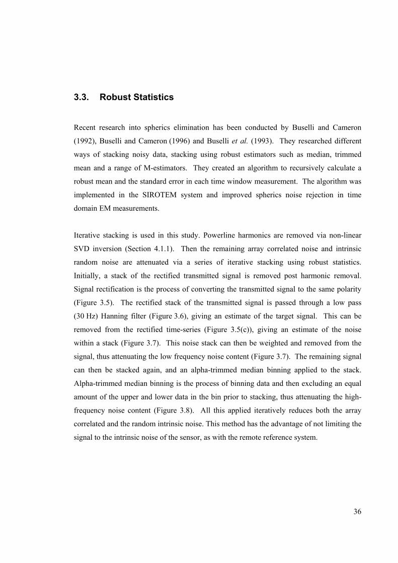
3.3. Robust Statistics
Recent research into spherics elimination has been conducted by Buselli and Cameron
(1992), Buselli and Cameron (1996) and Buselli et al. (1993). They researched different
ways of stacking noisy data, stacking using robust estimators such as median, trimmed
mean and a range of M-estimators. They created an algorithm to recursively calculate a
robust mean and the standard error in each time window measurement. The algorithm was
implemented in the SIROTEM system and improved spherics noise rejection in time
domain EM measurements.
Iterative stacking is used in this study. Powerline harmonics are removed via non-linear
SVD inversion (Section 4.1.1). Then the remaining array correlated noise and intrinsic
random noise are attenuated via a series of iterative stacking using robust statistics.
Initially, a stack of the rectified transmitted signal is removed post harmonic removal.
Signal rectification is the process of converting the transmitted signal to the same polarity
(Figure 3.5). The rectified stack of the transmitted signal is passed through a low pass
(30 Hz) Hanning filter (Figure 3.6), giving an estimate of the target signal. This can be
removed from the rectified time-series (Figure 3.5(c)), giving an estimate of the noise
within a stack (Figure 3.7). This noise stack can then be weighted and removed from the
signal, thus attenuating the low frequency noise content (Figure 3.7). The remaining signal
can then be stacked again, and an alpha-trimmed median binning applied to the stack.
Alpha-trimmed median binning is the process of binning data and then excluding an equal
amount of the upper and lower data in the bin prior to stacking, thus attenuating the high-
frequency noise content (Figure 3.8). All this applied iteratively reduces both the array
correlated and the random intrinsic noise. This method has the advantage of not limiting the
signal to the intrinsic noise of the sensor, as with the remote reference system.

37
Figure 3.5. Signal rectification. Time series (a) and its amplitude spectrum (b) is rectified to produce signal (c) and its amplitude spectrum (d). Rectification takes place by multiplying negative half-cycles by negative one.

38
Figure 3.6. Stacking prior to robust statistics and iterative stacking. The rectified signal (a) and its amplitude spectrum (b) have been binned and convolved with a low pass (30 Hz) Hanning filter, then logarithmically sampled, producing time series (c) and it’s amplitude spectrum (d). This binning provides a good estimate of the target signal for each sensor, which is removed prior to robust statistics and iterative stacking.

39
Figure 3.7. Robust statistics for removing low frequency noise. A stack of the transmitted signal is removed leaving a noise estimate (a) amplitude spectrum (b). The noise estimate for each sensor is stacked producing (c). This noise estimate is then weighted according to the RMS noise of individual sensor (e), this weighted stack of noise is removed from (a) producing (g).

40
Figure 3.8. Robust statistics as a means of removing high frequency noise. After low frequency noise removal, the noise estimate (a) remains. This remaining noise train is stacked with alpha trimmed median binning (which excludes the upper and lower 10% median values), producing (c). The signal estimate prior to low and high frequency noise attenuation is added to (c) producing (e).

41
4. Powerline Harmonics ________________________________________________________________________
Stationary sinusoidal noise, such as that generated from power distribution grids,
contaminates electromagnetic, induced polarisation, resistivity, magnetotelluric,
seismoelectric and seismic data. Other sources of this distinct frequency noise are
generators at mine sites or any rotating machinery. The base frequency of a the transmitted
electrical waveform is
n
hfbf = , (4.1)
where n is an even whole number and hf represents the local powerline transmission
frequency. This permits optimal powerline harmonic removal as synchronous averaging in
the time domain has a similar effect in reducing coherent noise as narrow band filtering in
the frequency domain. In Australia, the power transmission line is emitted at 50 Hz, though
in North America it is 60 Hz. The worst base frequencies to use are those that satisfy
nhfbf /= , where n is an odd whole number (Macnae et al., 1984; Spies and
Frischknecht, 1991; Nabighian and Macnae, 1991 and Duncan, 2002). Employing a
sensible base frequency is common practice for any electrical surveys, but it does not
completely remove harmonic noise and many other methods are in place to attenuate the
noise.
Traditionally notch filtering is used to remove these discrete frequency noise sources.
Notch filters deal with one frequency at a time and attenuates both the signal and noise at
the notch frequency. Notch filters and circuits to reject phase coherent cultural signals are
customarily included in a variety of modern exploration systems.

42
4.1. Inversion
Researchers have dealt with inversion techniques to solve for the phase and amplitude of
stationary sinusoidal noise after initially determining the sinusoidal frequency. This is done
by performing a search over a portion of the signal where the noise is strongest or there is
no transmitted signal. Nyman and Gaiser (1983), Griffith (1988) and Dragoset (1995) use
adaptive noise cancellation using least-mean squares. Linville and Meek (1992 and 1995)
and Butler and Russell (1993, 2003) and Butler et al. (1996) have developed linear least-
squares inversions. Xia and Miller (2000) use the Levenberg-Marquardt method with a
singular value decomposition (SVD) approach.
Powerline harmonics deviate from their fundamental frequency up to Error! Not a valid
embedded object. 0.03 Hz in developed countries, and up to Error! Not a valid
embedded object. 5 Hz in less developed countries. This is known as amplitude
modulation. The record length that traditional inversion techniques can operate on is
restricted. If the record length is too long residual harmonics will be left in the time series.
This is characterised by an increase in residual harmonics toward the end of the trace. The
same result will be observed if an incorrect fundamental frequency is selected for signal
processing. In the case of modulated harmonics, Butler and Russell (2003) suggest
estimating and including the appropriate side-bands as additional fundamentals.
Difficulties will be encountered in this method, for when modulation is a factor, the
amplitude of the side-bands of the fundamental frequencies are often hidden within the
lobes of the fundamental frequency peak and therefore not possible to estimate (Figure 2.8).

43
4.1.1. Non-Linear SVD Inversion for Modulated Harmonics
In this study the approach of non-linear SVD inversion is used for the removal of sinusoidal
noise. Sinusoidal noise with amplitude modulation is described in section 2.4.1. where
Equation (2.4) describes the behaviour of modulated powerline harmonic. There is a need
to invert for the amplitude and frequency of each harmonic and the amplitude and
frequency of the modulation envelope. However Equation (2.4) cannot be used as the
forward model, because it is highly non-linear and the inversion will not converge. Instead,
when modulation is dominant, the time series must be divided into multiple sections. The
harmonic noise with amplitude modulation maybe represented as the summation of
sinusoids with a quadratic function defining the modulation envelope as:
( ) ( )=
+++++=n
i
iiiiiiii tftdtcbtftdtcatmS1
22 )2cos()1(2sin1),( ππ, (4.2)
Where if is the frequency of the sinusoid, t is time, ia and ib are the amplitudes of the
sine and cosine components (the ratio of these is directly related to the phase of the
sinusoid), ic and id are the nominators of the quadratic amplitude modulation envelope
and n is the number of sinusoid functions needed to model the sinusoidal noise.
A SVD damped Gauss-Newton method is used to solve for the model parameters m as
[ ]nnnnn dcfbabadcfbam
2211111= , (4.3)
The forward model for the non-linear inversion is trivial. Therefore the Jacobian (A) is used
for inversion and is defined by the actual partial derivatives of S(m,t) with respect to the
model parameters.

44
∂∂
∂∂
∂∂
∂∂
∂∂=
iiiii dS
cS
fS
bS
aSA , (4.4)
where the size of A is equal to the length of the time series (or sections of) by (n×m), and
where;
)2sin()1( 2 tftdtcaS
iiii
π++=∂∂ , (4.5)
)2cos()1( 2 tftdtcbS
iiii
π++=∂∂ , (4.6)
( ) ( ) ttftdtcbttftdtcafS
iiiiiiiii
ππππ )2sin()1(22cos12 22 ++−++=∂∂
, (4.7)
)2cos()2sin( tftbtftacS
iiiii
ππ +=∂∂
, and (4.8)
)2cos()2sin( 22 tftbtftadS
iiiii
ππ +=∂∂
. (4.9)
The initial estimate of fi is a two stage process. A window of data from the time series is
selected. For most desirable results the windowed data contains only the sinusoidal noise
and the received signal, (i.e. noise from other sources is minimal). The transmitter signal is
calculated. In the amplitude spectrum, peaks which correlate with the transmitter signal
are set to nominal values. Window searches are conducted over the spectrum and the
indices of peaks which are greater than 2 times the mean of their window are selected as the
sinusoidal frequencies. The maximum peak and its neighbouring points are set to the mean,
and the window is searched again. This ensures that all sinusoidal frequencies are
accounted for (Figure 4.1).
These frequencies are then refined. The signal estimate is stripped from the time series and
a finer pick for the frequencies is made using the whole trace. In the amplitude spectrum

45
each initial frequency estimate is windowed, and the index of the maximum amplitude
within each window is selected as the frequency.
Utilizing the whole trace locates the frequency of the harmonic to ± 1/(total time of the time
series) (Figure 4.2). The initial approximations for ai and bi are completed by taking the
cross correlation of the time series with the sine and cosine components for each fi, ci and
di are initially set to zero for the idealistic non-modulation case.
The inversion for the model parameters is a two part process for each trace. The initial
inversion is carried out, then a weighted inversion, with weighting for each increment in the
time series, equal to 1/(residual noise remaining)2. This weighting reduces the influence of
the spherics on the inversion. The final estimates of the sinusoidal noise are subtracted
from the time series (Figure 4.3).

46
Figure 4.1. Harmonic noise removal the initial estimate the harmonic frequency, stage one. The transmitter response (b) and its amplitude spectrum (a) are used to estimate the received signal (d). Peaks in the amplitude spectrum of the transmitted signal will correlated with peaks in the amplitude spectrum of the received signal (c). These peaks can be trimmed to an average background value, producing (e), an estimate of the noise spectrum and the corresponding time series (f). This noise spectrum (e) can be used to estimate harmonic frequencies. The noise spectrum is broken up into small frequency ranges or windows, each window is analysed and frequencies where the peak amplitude is greater than 2 times the mean of the amplitudes in the window are selected as the sinusoidal frequencies.

47
Figure 4.2. Harmonic noise removal the initial estimate the harmonic frequency, stage two. Following the initial estimate of the harmonic frequencies (as seen in Figure 4.1). The frequency estimates are refined using all data from the time series for each individual sensor. An estimate of the received signal (d) and it’s amplitude spectrum (c) is obtained by stacking the signal received at all the sensors (b), with corresponding amplitude spectrum (a). The estimate of the received signal (d) and (c) are subtracted from (b) and (a) producing (f) and (e) an estimate of the remaining noise and it’s spectrum for the sensor. The frequencies which were selected in stage one (Figure 4.1) are windowed in the noise spectrum (e), the index of the maximum amplitude within the window is selected as the frequency. Utilizing the whole trace locates the frequency of the harmonic to ± 1/(total time of the time series).

48
Figure 4.3. Comparison of the received signal before and after powerline harmonic attenuation. The received time series (b) and its amplitude spectrum (a) in comparison to the received signal after harmonic removal (c) and its amplitude spectrum (d). Peaks in the amplitude spectrum (d) at 50 and 150 Hz, produced by powerline harmonics have been attenuated.

49
5. Array Processing ________________________________________________________________________
Data collected with a multi-sensor array has had little application in mineral exploration. In
1994, M.I.M Exploration Pty Ltd (MIMEX) designed and built a multichannel acquisition
system named MIMDAS (Mount Isa Mines’ distributed acquisition system). The foremost
approach using arrays for electrical methods in mineral exploration prior to MIMDAS was
the remote reference technique, where a second receiver is placed at a distance from the
target signal receiver and measurements are made simultaneously at both receivers. The
remote receiver can be used to estimate local noise sources, which can then be subtracted
from the target signal receiver. The remote reference must be placed far enough from the
transmitter (>10 km) that the observed remote fields consist only of geomagnetic
fluctuations. The remote receiver may be the same instrumentation as the target receiver.
Alternatively it can be a Supeconducting Quantum Iinterference Device (SQUID)
magnetometer. The technique extends low frequency (below 0.3 Hz base frequency) limits
by one decade.
When using a remote reference, there is significant distance between the target receiver and
the remote reference, therefore least-squares fit to find the transfer tensor between the target
receiver field components and the horizontal field components at the remote receiver is
performed before the noise can be subtracted. The tensor accounts for the lateral
conductivity change and relative alignment errors between the base and remote reference.
However, because the exact sensor relationship is frequency dependent and the power
spectra of geomagnetic noise change over a finite time intervals, there is no guarantee that
the coefficients calculated during an interval with the transmitter off will apply to data
collected during the transmitter on time.
Data is required to be gathered in short segments so that natural field drift can be offset for
each segment. The main limitation of this remote reference technique arises from the
quantisation errors of the receiver instrumentation. S/N improvement of roughly 20 dB is
expected (Wilt, et al., 1983).

50
Another possible scheme uses a symmetric receiver configuration in which the noise is
subtracted and the signal is added. This scheme is sensitive to alignment errors, as any
minimum coupled source receiver measurement, and could only be used in layered Earth
environments in which the signals would be mirror images at the two sites (e.g. San Filipo
and Hohmann, 1983).
Spies (1988), Buselli et al. (1995 and 1997) researched spherics elimination techniques
using a local noise prediction filter (LNPF) and a remote noise prediction filter (RNPF). A
LNPF predicts the vertical component of the spherics noise from the two horizontal
components. For a RNPF, noise is predicted for each component of spherics noise from
simultaneous three component measurements of spherics at a separate station. They found a
noise prediction filter can decrease the largest (horizontal) component of spherics noise by
a factor of 18, with the average noise reduction factor between 2 and 6.
Spies (1991) patented a cancelling antenna, which is wrapped around the sensing antenna
of the electromagnetic receiver equipment. The cancelling antenna is provided with an
alternating current signal of the same frequency as the ambient powerline noise. The
cancelling antenna produces an electromagnetic field that is 180 degrees out of phase and
of equal amplitude to the ambient powerline noise, as measured by the sensing antenna.
The alternating current is produced by a noise antenna, a phase-locked loop and an
amplifier. The noise antenna receives the ambient powerline noise, the phase-locked loop
locks onto and tracks the frequency of the noise, and the amplifier provides the necessary
amplification (Spies, 1991).
Stephan and Strack (1991) developed a method of noise reduction known as the local noise
compensation (LNC) technique. It is a noise cancellation technique for a multichannel far-
zone time-domain EM acquisition with dense station spacing. An estimate of noise at the
base station is calculated by removing a stacked estimate of the transient from each base
station period. This noise estimate is then removed from all receiver stations. To apply the
LNC, the following conditions must be met and tested at the beginning of the survey. The

51
noise must be correlated over a certain range around the base station, and this regional
noise cannot be reduced by standard processing. The receiver systems at the base station
and at the surrounding mobile stations must be identical in their system characteristics, and
the recording times in the data header must be synchronised to identify corresponding
records. The very localised noise belonging to only one receiver site (i.e. wind noise or
noise from nearby powerlines) must be smaller than the regional noise. In situations where
these conditions are met the, length of useable signal was increased by a factor of 10
(Stephan and Strack 1991).
Other disciplines, such as exploration seismology, passive sonar, radar, radio astronomy
and tomographic imaging, have looked at array signal processing techniques (Haykin Ed.,
1985, and Robinson, 1972). To date array processing has had limited application in
mineral geophysics. A comprehensive sequence of processing steps are shown here, which
apply both a non-linear SVD inversion for the removal of powerline harmonics, and
iterative stacking and robust statistics for the removal of array correlate noise and intrinsic
sensor noise.
The iterative stacking and robust statistics exploit the use of an array of sensors by using
the whole array to estimate the noise across the array, as data collected with a sensor array
consists of three main components:
1.Signal correlated with both the transmitter output and sensor array: the Earth
response, including the signal of interest and other geological influences.
2.Noise that is correlated within the sensor array, but uncorrelated with the transmitter:
harmonic noise (from the power grid) and atmospheric transients (spherics).
3.Noise that is both uncorrelated within the sensor array and to the transmitter output:
the random intrinsic noise of each sensor.
Using a sensor array, it is possible to recognise the different components received and
remove noise uncorrelated with the transmitter. There is increased coverage and resolution.
All data recorded is full waveform (both transmitter on and off time are recorded), this
ensures that no information is lost for any time. The use of multiple receiving sensors can
improve signal fidelity from each sensor, leading to more accurate geological models and

52
greater depth of investigation. Essentially all of the receivers behave as each other’s
remote references, though rather than getting a noise estimate from just one receiver, all of
the receivers in the array can be used to get an estimate of the correlated noise across the
array or an estimate of the transmitter correlated signal.
In this study the approach is to firstly remove the harmonic noise from each individual
sensor (Section 4.1.1) and then the remaining sensor array correlated noise is removed
using an iterative robust statistics stacking technique. The stacking consists of two steps.
The first attenuates the low frequency noise component and the second the high frequency
noise component (Section 3.3). Figure 5.1 shows the processing flow. This approach
effectively attenuates modulated harmonics, spherics and the random intrinsic noise of each
sensor. A significant advantage of this approach to compared to the remote reference
method is that it does not add the intrinsic noise of the remote reference to the data and a
sensor is not wasted.
Figures 5.2 to 5.4 show the application of the array processing workflow to three different
data sets. The IP and EM surveys recorded at Curtin University, and MIMDAS IP survey.
Details of these surveys can be found in Appendix 1.
The IP survey recorded at Curtin University (Figure 5.2) is strongly contaminated with
powerline noise. This is indicated in by the relatively wide peaks at 50 Hz and 150 Hz
which dominate the raw amplitude spectrum (Figure 5.2b). The inconsistent amplitude
envelope of the time series indicates that the powerline noise is modulated (non-linear)
(Figure 5.2a). After application of the non-linear SVD inversion for the attenuation of
powerline harmonics the peaks at 50 Hz and 150 Hz are removed from the amplitude
spectrum (Figure 5.2(d)). Following the array processing the only visible peaks in the
amplitude spectrum are due to the transmitted signal (Figure 5.2(f)). The signal to noise
improvement is a factor of 200.
Figure 5.3 shows the EM survey recorded at Curtin University. The time series show the
time decay for one recorded event (Figures 5.3(a), (c) and (e)). There is minor

53
contamination by harmonics, seen as small peaks in the amplitude spectrum in the locality
of 50Hz (Figure 5.3(b)). These are completely removed after application of the non-linear
SVD inversion is for the removal of sinusoidal noise (Figure 5.3(d)). The array processing
contributes the most to signal improvement with a dramatic improvement in decay curve
fidelity (Figure 5.3(e)).
Figure 5.4, the MIMDAS IP exploration example is contaminated with harmonics and
some other noise sources. Harmonic contamination is indicated by the presence of a peak
at 50Hz in the amplitude spectrum (Figure 5.4(b)). After array processing the final signal
to noise improvement is a factor of 30.

54
Figure 5.1. Array processing flow chart. The harmonic noise from each individual sensor using a non-linear SVD inversion for modulated harmonics (Section 4.1.1) and then the remaining sensor array correlated noise is removed using an iterative robust statistics stacking technique. The stacking consists of two steps. The first attenuates the low frequency noise component and the Figure 5.1. Array processing flow chart The harmonic noise from each individual sensor is attenuated using a non-linear SVD inversion for modulated harmonics (Section 4.1.1) and the remaining sensor array correlated noise is removed using an iterative robust statistics stacking technique. The stacking consists of two steps. The first attenuates the low frequency noise component and the second the high frequency noise component (Section 3.3).
Data recorded at sensor array
sensor
Inv
output

55
Figure 5.2. Array processing a field example: Curtin electrical data array processing. The initial time series (a) is contaminated with modulated harmonic noise, with the majority of the contamination from 150 and 50 Hz harmonics shown as spectral lines in (b). After SVD inversions to remove the harmonic frequencies the spectral peaks in the amplitude spectrum are greatly reduced (d) and the time series is more refined (c). Following harmonic removal the iterative robust statistics and alpha trimmed median stacking is applied producing (e). The amplitude spectrum is now predominately the transmitter correlated signal and there is a signal to noise improvement of 200. Details of the survey can be found in Appendix 1.

56
Figure 5.3. Array processing a field example: Curtin electromagnetic data array processing. Part of the initial time series (a) is shown, there is some subtle harmonic noise, indicated by a small peak at 50 Hz in the amplitude spectrum (b). After SVD inversions the 50 Hz peak is removed, as shown in amplitude spectrum (d), there is only slight change to times series (c). Following harmonic removal, iterative robust statistics and alpha trimmed median stacking is applied producing time series (e). Details of the survey can be found in Appendix 1.

57
Figure 5.4. Array processing a field example: MIMDAS data array processing, data courtesy of T. Ritchie, Xstrata Pty Ltd. The initial time series (a) is contaminated with modulated harmonic noise seen as a narrow spectral line at 50 Hz in amplitude spectrum (b). After SVD the 50 Hz spectral line is removed, as shown in amplitude spectrum (d) and the time series is uncontaminated (c). Following harmonic removal the time series is rectified then iterative robust statistics and alpha trimmed median stacking is applied producing the secondary field (e). There is a signal to noise improvement of 30. Details of the survey can be found in Appendix 1.

58
6. Conclusion and Recommendations ________________________________________________________________________
In this thesis I have analysed noise removal methods for electrical and electromagnetic time
series measurements. The study found that array processing is favourable to the remote
reference method, as each sensor in the array can be used to calculate the noise source
rather than just one or two sensors as in the remote reference method. It also showed a
multi-faceted approach to processing is beneficial. Chapter Three reviewed current
stacking techniques and demonstrated a processing flow using iterative stacking in
conjunction with robust statistics for S/N ratio improvement. Chapter Four reviewed
inversion techniques for powerline harmonic removal and demonstrated a superior
technique of SVD inversion which can remove modulated harmonics. Chapter Five
combined an array processing flow which incorporated SVD inversion for the removal of
modulated harmonics in conjunction with iterative stacking and robust statistics. The
processing flow was applied to field examples of electrical and electromagnetic data,
collected in both cultural and exploration environments. In areas where data was highly
contaminated with cultural noise signal to noise ratio improvements of 200 were observed.
These multifaceted array processing techniques lead to much improved signal to noise
(greater then 46 dB), which ultimately leads to greater signal fidelity and greater depths of
investigation.
Chapter Three reviewed pre-whitening/pre-emphasis and showed a method of spiking
deconvolution for spherics removal. Spiking deconvolution as a method of spheric removal
proved flawed. One of the caveats for spiking deconvolution is that the inverse of the
deconvolution operator, the spheric event, should be minimum phase. A local spheric event
will be minimum phase, but as the distance from the source increases and/or more than one
spheric event arrive in the same time window, the minimum phase assumption fails and so
does the method.
This research is a foreword to the yet greatly unexplored area of array processing for
electrical and electromagnetic time series. Great gains can be made by intelligent use of

59
any array of sensors and many processing applications are still to be explored. There is
advantage to reviewing existing processing methods in the seismic data processing
industry, which has an established history for array processing.

60
References ________________________________________________________________________
Asten, M. W., 1987, Full transmitter waveform transient electromagnetic modeling and inversion for soundings over coal measures: Geophysics, 52, 279-288. Becker, A., and Cheng, G., 1987, Detection of repetitive electromagnetic signals, in Nabighian, M. N., Ed., Electromagnetic methods in applied geophysics: Soc. Expl. Geophys., 1, 443-466. Buselli, G. and Cameron, M.A., 1992, Improved spherics reduction in TEM measurements,” CSIRO Division of Exploration Geoscience, Restricted Report 273R (now on open file), p. 60. Buselli, G. and Cameron, M.A., 1993, Final report for AMIRA Project P250A: Improved TEM detection of massive sulphide orebodies, Restricted Report 350R (now on open file), p. 29. Buselli, G., and Cameron, M., 1996, Robust statistical methods for reducing sferics noise contaminating transient electromagnetic measurements: Geophysics, 61, 1633-1646. Buselli, G., Hwang, H.S., and Pik, J.P., 1995, Sferics elimination progress report, CSIRO Division of Exploration and Mining Report 116R, p.46 Buselli, G., Hwang H. S., and Pik, P., 1997, Final report on the sferics elimination module of AMIRA project P407,. CSIRO exploration and mining report 294R. Butler, K. E., and Russell, R. D., 1993, Subtraction of powerline harmonics from geophysical records: Geophysics, 58, 898-903. Butler, K. E., Russell, R. D., Kepic, A. W., and Maxwell, M., 1996, Measurement of the seismoelectric response from a shallow boundary: Geophysics, 61, 1769-1778. Butler, K. E., and Russell, R. D., 2003, Cancellation of multiple harmonic noise series in geophysical records: Geophysics, 68, 1083-1090. Duncan, A., 2002, SMARTem electrical methods receiver system: Electromagnetic Imaging Technology. Dragoset, B., 1995, Geophysical applications of adaptive noise cancellation: 65th Ann. Internat. Mtg., Soc. Expl. Geophys., Expanded Abstracts, 1389-1392. Garner, S. J., and Thiel, D. V., 2000, Broadband (ULF-VLF) surface impedance measurements using MIMDAS, Exploration Geophysics, 31, 173-178.

61
Griffith, P. G., 1988, Nonlinear quadrature noise canceling of narrow band signals in seismic data: 58th Ann. Internat. Mtg., Soc. Expl. Geophys., Expanded Abstracts, 1270-1274. Haykin, S., 1985, Radar array processing for angle arrival estimation: Array Signal Processing, Haykin, S. (ed), Prentice-Hall, Englewood Cliffs, NJ, Chapter 4. Jewell, T. R., and Ward, S. H., 1963, The influence of conductivity inhomogeneities upon audio-frequency magnetic fields: Geophysics, 28, 201-221. Kaufman, A. A., and Keller, G. V., 1983, Frequency and transient soundings: Elseveier Science Publ. Co. Inc. Lee, T., and Lewis, R., 1974, Transient response of a large loop on a layered ground: Geophys. Prosp., 22, 430-444. Linville, A. F., and Meek, R. A., 1992, Cancelling stationary sinusoidal noise; Geophysics, 57, 1493-1501. Linville, A. F., and Meek, R. A., 1995, A procedure for optimally removing localized coherent noise; Geophysics, 60, 191-203. Macnae, J. C., Lamontagne, Y., and West, G. F., 1984, Noise processing techniques for time-domain EM systems: Geophysics, 49, 934-948. McCracken, K.G., Oristaglio, M.L. and Hohmann, G.W., 1986b. Minimization of noise in electromagnetic exploration systems: Geophysicis, 51, 819-832. McCracken, K. G., Pik, J. P., and Harris, R. W., 1984, Noise in EM exploration systems: Exploration Geophysics, 15, 169-174. McNeill, J. D., and Labson, V., 1991, Geological mapping using VLF radio fields, in Nabighian, M. N., Ed., Electromagnetic methods in applied geophysics: Soc. Expl. Geophys., 2, 521-640. McPherron, R. L., 2002, Magnetic pulsations: their sources and relation to solar wind and geomagnetic activity: 16th EM Induction Workshop. College of Santa Fe., Workshop Papers. Nagibhian, M. N., and Macnae, J. C., 1991, Time domain electromagnetic prospecting methods, in Nabighian, M. N., Ed., Electromagnetic methods in applied geophysics: Soc. Expl. Geophys., 2, 427-520. Nyman, D. C., and Gaiser, J. E., 1983, Adaptive rejection of high-line contamination: 53rd Ann. Internat. Mtg., Soc. Expl. Geophys., Expanded Abstracts, 1270-1274.

62
Parasnis, D. S., 1997, Principles of applied geophysics: Chapman & Hall. Ritchie, T., 2003, personal communication. Ryan. A., and Scranton. T., 1984, D-C amplifier noise revisited: Analog Dialogue, 18, 151-159. San Filipo, W. A., and Hohmann, G. W., 1983, Computer simulation of low-frequency electromagnetic data acquisition, Geophysics, 48, 1219-1232. Sheriff, R. E., 1999, Encyclopedic dictionary of exploration geophysics: Soc. Expl. Geophys. Smith, L., and Sheingold, D. H., 1969, Noise and operational amplifier circuits: Analog Dialogue, 3, 19-31. Spies, B. R., 1988, Local noise prediction filtering for central induction transient electromagnetic sounding: Geophysics, 53, 1068-1079. Spies, B. R., 1991, Method and apparatus for cancelling powerline noise in geophysical electromagnetic exploration: United States Patent 4996484. Spies, B. R., and Frischknecht, F. C., 1991, Electromagnetic sounding, in Nabighian, M. N., Ed., Electromagnetic methods in applied geophysics: Soc. Expl. Geophys., 2, 285-425. Stephan, A., and Strack, K. M., 1991, A simple approach to improve the S/N ratio for TEM data using multiple receivers: Geophysics, 56, 863-869. West, G. F., and Macnae, J. C., 1991, Physics of the electromagnetic induction exploration method, in Nabighian, M. N., Ed., Electromagnetic methods in applied geophysics: Soc. Expl. Geophys., 2, 5-45. White, R. M. S., Collins, S., Denne, R., Hee, R., and Brown, P, 2001, A new survey design for 3D IP inversion modelling at Copper Hill, Exploration Geophysics, 32 , 152-155. Wilt, M., Goldstein, N. E., Stark, M., Haught, J. R., and Morrison, H. F., Experience with the EM-60 electromagnetic system for geothermal exploration in Nevada: Geophysics, 48, 1090-1101. Xia, J., and Miller, R. D., 2000, Design of a hum filter for suppressing power-line noise in seismic data: Journal of Environmental and Engineering Geophysics, 5, 31-38. Yilmaz, O., 2001, Seismic data analysis: Soc. Expl. Geophys.

63
Zonge, K. L., and Hughes, L. J., 1991, Controlled source audio-frequency magnetotellurics, in Nabighian, M. N., Ed., Electromagnetic methods in applied geophysics: Soc. Expl. Geophys., 2, 713-810.
Every reasonable effort has been made to acknowledge the owners of copyright material. I
would be pleased to hear from any copyright owner who as been omitted or incorrectly
acknowledged.

64
Appendix 1. Data Acquisition ________________________________________________________________________
All data recorded is full waveform both transmitter on and off time are recorded. The data
was with multiple receivers and recorded simultaneously in time at each sensor. The
premise is data collected with a sensor array consists of three main components:
1.Signal correlated with both the transmitter output and sensor array: the earth
response, including the signal of interest and other geological influences.
2.Noise that is correlated within the sensor array, but uncorrelated with the transmitter:
harmonic noise (from the power grid) and atmospheric transients (spherics).
3.Noise that is both uncorrelated within the sensor array and to the transmitter output:
the random intrinsic noise of each sensor.
Using a mutliple sensor array, it is possible to recognise the different components received
and remove noise uncorrelated with the transmitter. Three multiple sensor field surveys are
presented: MIMDAS IP, IP Survey ar Curtin University and EM survey at Curtin
University. The MIMDAS IP is an exploration dataset and the Curtin datasets were
recorded in an urban environment. The MIMDAS IP data was provided by Terry Ritchie,
MIM Exploration Pty Ltd (now Xstrata Plc). Streaming noise data, Noise Darwin, was
provided by Jock Buselli, CSIRO Exploration and Mining, originally recorded on magnetic
tape with an analogue tape recorder.
1A. MIMDAS IP An exploration example: IP data were collected with MIM Exploration’s (now Xstrata)
proprietary distributed acquisition system “MIMDAS”. MIMDAS, is a broadband, high
resolution, distributed (multi-channel) acquisition system. MIMDAS is designed to acquire
networked multi-channel electrical and EM geophysical data, though it could be used to
acquire seismic data. Each channel or data acquisition unit (DAU) is networked in series
with a computer interfaced central recording unit (CRU) and is capable of capturing

65
250,000 samples or 1 Mb of data at many hardware specific, but software selectable,
sample rates. MIMDAS has four gain settings and is capable of 24-bit resolution at sample
rates up to 4800 Hz and 19-bit resolution from 4800 Hz to 48 kHz inclusive (Garner and
Thiel, 2000). For the IP-MIMDAS data the transmitter used a 100 % duty cycle waveform
with peak-to-peak amplitude 13.7 A, base frequency of 0.0977 Hz, sampling frequency
200 Hz and a total of 32 stacks for each recording. There were 84 diploes 100 m apart with
line spacing of 200 m covering a survey area 1.4 km by 1 km.
1B. IP Survey at Curtin University Urban Example: A simulated low power electrical/IP survey was conducted in Perth,
Western Australia. A transmitter with a 50 % duty cycle waveform with, base frequency of
3.125 Hz, injected current with a peak-to-peak amplitude of 34 mA into the ground with a
5 m grounded dipole. There were a total of 30 stacks. The receiving system consisted of
24 grounded dipoles (spacing 1 m), located 10 m from the transmitter, connected to AC
coupled pre-amplifiers (each with a gain of 30) relayed to an OYO DAS-1 seismic
acquisition system with a sampling frequency of 500 Hz. The AC coupled amplifiers in the
OYO DAS-1 and the preamplifiers remove low frequencies in the signal, thus, simulating a
signal that might be received by an IP/EM system.
1C. EM Survey at Curtin University
Urban Example: A NanoTEM NT-20/2T transmitter with a 50 % duty cycle waveform with
base frequency of 4.166 Hz, total of 130 stacks, injected current with a peak-to-peak
amplitude of 3.2 A via a 100 m by 100 m transmitter loop. The receiving system consisted
of 8 scalar receivers in-loop, with areas 10000 m2, the receivers were developed in house
by Anton Kepic and are known as Curtin University of Technology Coils (CUT). The
receivers were connected to AC coupled pre-amplifiers (each with a gain of 30) relayed to
SMARTem acquisition system with a sampling frequency of 10000 Hz.

66
1D. Noise Recording in Darwin Noise Example: Three data sets were provided by Jock Buselli of CSIRO. Data were
recorded on magnetic tape with an analogue tape recorder. Data were then digitised and
recorded on a cassette tape, and later transferred to CD. Data were recorded in Darwin,
February 1983. Sampling frequency was 20000 Hz, the receivers consisted of two100 m by
100 m surface loops with gain 10 (20 dB) and gain 100 (40 dB), and a z-component scalar
receiver with area 10000 m2, with gain 100 (40 dB).
Recommended