Louisiana State UniversityLSU Digital Commons

LSU Doctoral Dissertations Graduate School

2009

Temperature impact on nitrification and bacterialgrowth kinetics in acclimating recirculatingaquaculture systems biofiltersMilton Maada-Gomoh SaiduLouisiana State University and Agricultural and Mechanical College, maadasaidu@hotmail.com

Follow this and additional works at: https://digitalcommons.lsu.edu/gradschool_dissertations

Part of the Engineering Science and Materials Commons

This Dissertation is brought to you for free and open access by the Graduate School at LSU Digital Commons. It has been accepted for inclusion inLSU Doctoral Dissertations by an authorized graduate school editor of LSU Digital Commons. For more information, please contactgradetd@lsu.edu.

Recommended CitationSaidu, Milton Maada-Gomoh, "Temperature impact on nitrification and bacterial growth kinetics in acclimating recirculatingaquaculture systems biofilters" (2009). LSU Doctoral Dissertations. 37.https://digitalcommons.lsu.edu/gradschool_dissertations/37

TEMPERATURE IMPACT ON NITRIFICATION AND BACTERIAL GROWTH KINETICS IN ACCLIMATING RECIRCULATING

AQUACULTURE SYSTEMS BIOFILTERS

A Dissertation

Submitted to the Graduate Faculty of the Louisiana State University and

Agricultural and Mechanical College in partial fulfillment of the

requirements for the degree of Doctor of Philosophy

In

The Interdepartmental Program in Engineering Science

By

Milton Maada-Gomoh Saidu. B.S. University of Sierra Leone, 2001 M.S. Louisiana State University, 2004

August, 2009

ii

Acknowledgements

I acknowledge the support, assistance, inspiration and advice of many individuals during

my Ph.D. studies at Louisiana State University. My gratitude goes to Dr. Steven Hall, my major

advisor for his willingness to accept me into the program and working with me to the end. He is

a family man and a good mentor who coached me spiritually and academically. He has been the

quiet guardian through thick and thin, always spurring me on. Thanks to Dr. Ronald Malone for

his open door policy and humble professionalism that has been significantly beneficial to me

through my program. I especially appreciate his willingness to go out on a limb to encourage

students who may feel down when research is not headed in the right direction. Dr. Terry Tiersch

offered advice and a research laboratory for this study. He always showed willingness to edit

drafts of scientific materials amidst his busy schedule. I respect his boldness to share what he

believes in and his objectivity on issues pertinent to progress.

Thanks to Dr. Aghazadeh for his positive views for success in life and believing in me to

go through this program. Thanks to Prof. Sharky and Dr. Justis for their encouraging views and

for serving on my committee. I would also like to thank Rebecca Schramm for bringing me into

her family and being supportive, Mrs. Rebecca Hall for opening her home to me and Mrs. Sandy

Malone for all her support and encouraging words. Special thanks to Angela Singleton, Rhonda

Shepard and Donna Elisar for all the paper work and office support I needed through my study.

Thanks to my academic colleagues Jack Chiu, Deepti Salvi, Jose Deras, Jason Midgett and

Carlos Astete with whom I sought late night technical advice during my experiments. A special

thanks to Tom McClure for his support in the system design, and to Jeremy Birch for his support

in my wiring layout and system design. There are many more worthy of acknowledgement, I

thank you all. It has been a pleasure considering those who have been by my side through it all.

iii

May God bless you all. I thank God above all for bringing me to this stage of my life. This

research was supported partly by Sea Grant, and Louisiana State University, Agricultural and

Biological Engineering Department and the College of Engineering.

iv

Table of Contents Acknowledgements ...................................................................................................................... ii List of Tables ............................................................................................................................... vii List of Figures ............................................................................................................................. viii Abstract ...........................................................................................................................................x Chapter 1 – Overview ....................................................................................................................1 1.1 References ......................................................................................................................7 Chapter 2 - Introduction ..............................................................................................................9

2.1 Biofilters. .......................................................................................................................9 2.2 Biofilm ........................................................................................................................10 2.3 Characteristics of Filters ............................................................................................. 12

2.4 Fluidized Bed Flow ......................................................................................................13 2.5 Bead Filters ..................................................................................................................14 2.6 Attached Growth ..........................................................................................................15 2.7 Nitrification ..................................................................................................................16 2.8 Estimating Ammonia Removal Rates ..........................................................................18 2.9 Factors Affecting Nitrification Rates ...........................................................................20 2.9.1 Dissolved Oxygen ..............................................................................................20 2.9.2 Total Ammonia Nitrogen ...................................................................................21 2.9.3 Effects of pH on Nitrification ............................................................................22 2.9.4 Alkalinity ...........................................................................................................23 2.9.5 Organic Loading ................................................................................................23 2.9.6 Temperature .......................................................................................................24 2.10 References ..................................................................................................................27

Chapter 3 – Temperature Effect on Biofilter Total Ammonia Nitrogen Removal Rate Performance ..........................................................................................................33 3.1 Introduction .................................................................................................................33 3.2 Background ..................................................................................................................34

3.3 Materials and Methods. ................................................................................................37 3.3.1 Biofilter Bead Acclimation ...............................................................................40 3.3.2 Systems Sanitization ......................................................................................... 41

3.3.3 Temperature Control and Data Acquisition .......................................................42 3.3.4 Experimental Design and Sample Analysis .......................................................43

3.4 Results and Discussion ................................................................................................46 3.4.1 Steady State Temperature (13, 20 & 30oC) Ammonia Removal Rates .............46

3.4.2 Diurnal Temperature (20 ± 3oC and 30 ± 3oC) Ammonia Removal Rates ........49 3.4.3 Diurnal Temperature (20 ± 3oC and 30 ± 3oC) Ammonia Removal Rates

with Mixed Beads ..............................................................................................51

v

3.4.4 Ammonia Removal Rate at Step-down Temperature (30 Step down-13oC)......................................................................................52

3.4.5 Ammonia Removal Rate at Step-up Temperature (13 Step up-30oC). ..............55 3.4.6 Comparison of Ammonia Removal Rates ........................................................56

3.5 Conclusions ................................................................................................................. 66 3.6 References ....................................................................................................................67

Chapter 4- Simulation Modeling of Temperature Effect on Bacterial Growth Phase Biofiltration Processes .............................................................................................70 4.1 Introduction ..................................................................................................................70

4.2 Background. .................................................................................................................71 4.3 Materials and Methods .................................................................................................73 4.3.1 Modeling Theory ...............................................................................................74

4.3.2 Modeling Structure and Implementation ...........................................................75 4.3.3 Modeling Assumptions and Verification ...........................................................77 4.4 Modeling Results .........................................................................................................77

4.4.1 Model and Observed Data at 13, 20 and 30oC ...................................................78 4.4.2 Model and Observed Data at 20 ± 3 and 30 ± 3oC ............................................80 4.4.3 Model and Observed Data at 20 ± 3 and 30 ± 3oC (Mixed Beads) ...................81

4.4.4 Sensitivity Analysis ...........................................................................................83 4.5 Discussion ....................................................................................................................85

4.6 Conclusions ..................................................................................................................87 4.7 References ....................................................................................................................88 Chapter 5- Summary and Conclusions ......................................................................................90

5.1 References ...................................................................................................................96 Appendix A- Protocol for Loading Tanks with Synthetic Nutrient (Ammonia) Water........98 Appendix B- Synthetic Nutrient (Ammonia –Nitrogen) Mixture for the Tanks ...................99 Appendix C- Steps to Change Temperature of Controlled Tanks ........................................100 Appendix D- Steps to Change Transient Temperature (Sine-Wave) Deviations .................101 Appendix E- Biofilter Sizing and Filter Design Characteristics ............................................102 Appendix F- Filter Preparation and Sampling .......................................................................104 Appendix G- Wiring Color Code for Temperature Control Relay Boxes ............................105 Appendix H- BAE Engineering Laboratory- Relay Schematics ...........................................106 Appendix I- Calculations for Standard Dilutions and Standard Curve Plot .......................107

vi

Appendix J- Design and Testing of Laboratory Temperature Control Batch Tank System ...............................................................................................................................109 Appendix K- Determining Order of Reaction Kinetic from data plot ..................................147 Appendix L- Comparison of Mean Concentrations for Steady State Diurnal and Mixed Bead at Diurnal Regimes ...........................................................................................................151 Appendix M- Installation, Configuration and Operation of Data Acquisition System (DAS) Boards .........................................................................................................................................160 Appendix N- Letter of Permission ............................................................................................179 Vita ..............................................................................................................................................180

vii

List of Tables Table 1.1: Conference presentation and abstracts based on research presented in the document….. ....................................................................................................................................6 Table 1.2 Published articles and manuscripts in preparation based on the research presented in this dissertation ................................................................................................................................7 Table 3.1: Chemical composition of substrate nutrients: (Wortman and Wheaton, 1991) ...........40 Table 3.2: Thirty-six tank layout shows nine tanks in the top row which were randomized for the experiments. A T,x,y configuration was used such that T is temperature (13, 20 and 30oC; 20 ± 3oC and 20 ± 3oC) x is the row and y is the tank number in that column. .....................................44

Table 3.3: Vmax (Specific Removal Rate), R2 and t values at the steady state, diurnal and step regimes ...........................................................................................................................................53 Table 4.1: Parameter values used in the model compared to literature .........................................76 Table 4.2a, 4.2b & 4.2c: Sensitivity analysis parameter percentage changes ..............................84

viii

List of Figures Figure 1.1: The nitrogen cycle in a natural ecosystem: This shows ammonia conversion to nitrite and nitrate.........................................................................................................................................3 Figure 2.1: Uniform flow distribution of water from base of media. (U.S. Patent No. 5,232,586 by Ronald Malone, Department of Civil Engineering, Louisiana State University) .....................14 Figure 2.2: A Michaelis Menten graph of reaction kinetics (Recirculating Aquaculture Systems; Timmons et al., 2002; Timmons and Ebeling, 2007) ....................................................................20 Figure 3.1: Enhanced nitrification media in the bacteria culture tank ..........................................39 Figure 3.2: Fiberglass nutrient mixing tank (0.91 m in diameter- Total volume ≈ 500 L) ...........39

Figure 3.3: Biofilter at one end of tank with airlift for water circulation .....................................40 Figure 3.4: Individual tanks with all components (pump, biofilter, thermocouple and heater) ....42 Figure 3.5: Typical approaches to steady state temperature profiles for 13, 20 and 30oC ...........47 Figure 3.6: Steady state 13, 20 and 30oC mean ammonia (TAN) concentrations of the biofilters and S1 is the initial solution concentration normalized to 5 gm-3..................................................48 Figure 3.7: Graph of volumetric total ammonia nitrogen removal rates at steady state (13, 20 and 30oC) regimes.................................................................................................................................49 Figure 3.8: Graph shows biofilter performance t with increase in steady state temperature profiles 13, 20 and 30oC.................................................................................................................50 Figure 3.9: Typical diurnal temperature profiles at 20 ± 3oC and 30 ± 3oC .................................50 Figure 3.10: TAN mean ammonia concentrations at diurnal (20 ± 3 and 30 ± 3) regimes ..........51 Figure 3.11: Volumetric TAN removal rates at diurnal (20 ± 3 and 30 ± 3) temperature regimes ...........................................................................................................................................52 Figure 3.12: TAN volumetric removal rates for diurnal temperatures (20 ± 3 and 30 ± 3) with mixed beads ...................................................................................................................................53 Figure 3.13: Step temperature TAN mean concentration at 30-13 degree step-down regime ......54 Figure 3.14: Volumetric TAN removal rate at step-down (30-13) regime ...................................54 Figure 3.15: Step temperature TAN mean concentration at 13-30oC degree step-up regime ......55

ix

Figure 3.16: Volumetric TAN removal rates at step temperature regimes (13-30oC) ..................56 Figure 3.17: Mean TAN concentration removal rates at 13-30 Vs 30oC ......................................57 Figure 3.18: TAN mean concentration removal rates at 30-13 Vs 13oC ......................................57 Figure 3.19: TAN mean concentrations at 20 Vs 20 ± 3oC diurnal temperature regimes ............59

Figure 3.20: TAN mean concentrations at 30 Vs 30 ± 3oC diurnal temperature regimes ............60 Figure 3.21: TAN mean concentrations at 20 Vs 20 ± 3oC diurnal temperature regimes using mixed beads ...................................................................................................................................61 Figure 3.22: TAN mean concentrations at 30 Vs 30 ± 3oC diurnal temperature regimes using mixed beads ...................................................................................................................................61 Figure 3.23: TAN mean concentrations removal rate at 20 ± 3oC transient Vs 20 ± 3oC diurnal mixed beads .......................................................................................................................63 Figure 3.24: Ammonia conversion at 30 ± 3oC diurnal Vs 30 ± 3oC mixed bead diurnal regime ............................................................................................................................................63 Figure 4.1: Generalized bacterial growth curve showing the phases in the growth of bacterial colonies from inoculation in medium to steady state biofilm ........................................................71 Figure 4.2: Model construct with input parameters in a batch reaction system ............................75 Figure 4.3: Graph of observed data versus simulated data for 13, 20 and 300C temperature regimes ...........................................................................................................................................78

Figure 4.4: Graph of bacterial mass from simulated data 13, 20, and 300C .................................79 Figure 4.5: Graph of observed data versus simulated curves for 20 ± 3 and 20 ± 3oC .................80 Figure 4.6: Graph of bacterial mass from simulated data 20 ± 3 and 30 ± 3 0C ...........................81 Figure 4.7: Graph of observed data versus simulated curves for 20 ± 3 and 30 ± 3oC (Mixed Beads) ................................................................................................................................82 Figure 4.8: Graph of bacterial mass from simulated data 20 ± 3 and 30 ± 3 0C (Mixed Beads) ................................................................................................................................82

x

Abstract

This project assessed short-term temperature effects on total ammonia nitrogen (TAN)

utilization rates in a batch laboratory-scale recirculating system. The tank system was designed

for experiments on short term steady state and diurnal temperatures. A set of numerical models

was developed to simulate observed results. The performance of the biofilters was determined

with three tank replicates at fixed temperatures of 13, 20 and 300C; and at diurnal transient

(sinusoidal) temperature regimes of (20 ± 30C; 30 ± 30C). Ammonia utilization rates and biofilter

performance for beads acclimated at different temperatures regimes separated and mixed were

also determined.

Total ammonia utilization rates increased with increased temperatures. The ammonia

removal rates (Pseudo Zero Order) with slope (K) did not significantly differ (P > 0.05) for 130C

(K = -0.02) and 200 C (K = -0.04); but differed (P < 0.05) for 13 and 300C (K = -0.12) and also

differed (P<0.05) for 200C and 300C. Diurnal temperatures values differed (P = 0.001) for 200C

± 30C (K = -0.08) and 300C ± 30C (K = -0.19). Ammonia utilization rate values for beads that

were acclimated and mixed at temperatures of 13, 20, 300C and subjected to diurnal temperatures

differed (P = 0.024) at 200C ± 30C (K = -0.12); and 300C ± 30C (K = -0.36). Biofilter

performance increased with temperature linearly with increased performance occurring at higher

temperatures and high bacterial mass.

Ammonia utilization rate simulated models matched the observed data and assisted in

determination of bacterial mass. Future designs and acclimation of the bead filters may be further

enhanced by decreasing biofilter acclimation periods using higher temperatures in recirculating

systems.

Keywords: ammonia nitrogen, temperature regime, bacteria, recirculating systems, aquaculture, biofilters, process control and nitrification.

1 

Chapter 1: Overview

Information on biofiltration and bacterial effect on biofilter performance is important to

the contributions of growth in aquaculture production. Recent growth in US and world

aquaculture is attributed to: (1) human population increase; (2) limited expansion or losses of

traditional fisheries; (3) increased demand for high protein; and (4) emphasis on healthy low fat

foods (Wortman and Wheaton, 1991). Consequently per capita fishery consumption has

increased in the US nearly 30% since 1990. The increased consumption has outpaced beef and

pork with aquaculture production accounting for 11% of sea food consumed in the last decade

(Wortman and Wheaton, 1991). In 2005, consumption increased such that more than 38% of all

seafood consumed around the world was produced by aquaculture (Timmons and Ebeling, 2007;

USDA, 2008). Although aquaculture is still in its emergent phase in the US, one aspect of

aquaculture that is contributing to production is closed-cycle (recirculating) systems. Closed-

cycle systems essentially utilized water in a recycled manner which helps to conserve water, a

global natural resource.

Global concern about water resources becoming limited, including the rising cost of pre-

treatment and post-treatment of water, have favored applications of water reuse and

reconditioning technologies (Watten et. al, 2004; Lyssenko and Wheaton, 2006, Timmons and

Ebeling, 2007). Water reuse has led to emerging technologies for improving water quality in

closed recirculation systems. Improved water quality also minimizes discharge of toxic effluent

from recirculation systems. Improving water quality in recirculating systems conserves water

resources. Aquaculture has contributed to increased demand for water (Wortman and Wheaton,

1991) in the United States to meet high protein demand from consumers of fish. Recirculation

systems treat water that deteriorates in quality over time from feeding the cultured species. The

water treatment involves multiple processes including recirculation of water through the biofilter

2 

to remove toxic nitrogenous waste and eventually some small discharge of waste water. The

effluents from these systems usually contain waste including nitrogenous waste (NH3, NO2 and

NO3), total suspended solids (TSS), biochemical oxygen demand (BOD) and chemical oxygen

demand (COD). The effects of these effluents after treatment remain a concern for productivity

of the systems and the environment in general.

The key focus of treating water in recirculation systems is a two-step ammonia removal

microbial filtration process called nitrification (Kim, et al., 2006; Sousa and Foresti, 1996 and

Carvantes et al., 2001). The process of ammonia removal is usually quantified in terms of

nitrogen content of the nutrient removed from the system. The first step in the ammonia nitrogen

removal process is the aerobic oxidation of ammonia to nitrite, and then to nitrate. The process is

performed by ammonia oxidizing bacteria (AOB) called nitrifying bacteria, which get their

energy from the oxidation of nitrogen compounds. The bacteria convert ammonia to nitrite

(Wiesmann, 1994; Tanwar et al., 2007). Another group of bacteria in the system use nitrite as an

electron acceptor to convert nitrite to nitrate (Zeng et al., 2003; Lucas et al., 2005). The process

thus converts the nitrogen compound ammonia to nitrate a less toxic form in a recirculation

system and eventually to N2 gas as in a natural ecosystem (Figure 1.1). The less toxic nitrate

nitrogen water in the recirculation system could then be diluted or discharged to surface waters.

Discharged nitrogen is of great concern in natural ecosystems (Jorgensen and Halling-

Sorensen, 1993) considering the fact that nitrogen (a) contributes to eutrophication (Loehr,

1984); (b) increases oxygen demand due to oxidation of organic and reduced forms of inorganic

nitrogen; and thirdly (c) has a toxic potential in certain forms which is harmful to aquatic species

including brown blood disease in fish (Lawson, 1995). This is a major concern of this study in

reducing the concentrations to levels that will be less toxic to fish raised in recirculating

3 

Figure 1.1: The nitrogen cycle in a natural ecosystem: This shows ammonia conversion to nitrite and nitrate.

aquaculture systems. In recirculating aquaculture systems nitrogen is produced by the fish

through their metabolic process using protein and the accumulation of the nitrogen is controlled

to prevent toxicity. A key nitrogen management practice in recirculation systems is to pass the

water through a biofiltration system (Greiner and Timmons, 1998) to reduce the concentration to

acceptable levels. The process is normally influenced by factors such as biochemical oxygen

demand (BOD), pH, oxygen and temperature (Manthe et al., 1988; Michaud et al., 2006).

The influence of temperature in the nitrification process in a recirculating aquaculture

system could help or harm production. Control of the production environment, leads to

advantages such as uniform quality products, limited water use and the ability to grow fresh

products (Wortman and Wheaton, 1991; Timmons and Ebeling, 2007). In addition to the

advantages of control for production of fresh products, temperature control could also enhance

4 

the removal of ammonia and other nitrogen compounds. Controlling the nitrification process

could increase production volume, reduce discharged water and enhanced profitability for system

managers.

The advantages mentioned above could be achieved if effects of temperature control on

the nitrification process could be further explored. The current goal was to contribute to ongoing

work in the area of temperature and nitrification interaction predictions for recirculating

aquaculture systems. The research reported here utilized comparative studies of ammonia

removal rates at different temperature regimes using bench scale biofilters in laboratory scale

tank systems. This research also develops a frame work for commercially adopting temperature

impacts on biofiltration to improve production.

The objectives were to: 1) determine ammonia removal rates at steady state temperature

regimes; 2) determine ammonia removal rates during diurnal temperature regimes; 3) determine

ammonia removal rate at diurnal temperatures, with mixed acclimated media (where mixed

acclimated media refers to media that was acclimated at different temperature regimes prior to

mixing); 4) determine ammonia removal rates at step-up (raising temperature from a lower to a

higher value) regime and step-down (dropping temperature from a higher to a lower value) and

5) model the process to predict biofilter performance and to enhance future design.

The results presented in this dissertation call attention to the requirement for researchers

to standardize ammonia removal in recirculation systems including acclimation and temperature

variations. Currently, recirculating systems and wastewater treatment plants are the leading areas

of biofiltration application with considerations for temperature. The most important steps in

determining biofiltration performance in a recirculation system are sizing, designing &

construction of the system components and understanding temperature effects.

5 

The research in this dissertation involved constructing a laboratory scale self-contained

system of tanks that were use to perform the experiment. One of the earliest efforts in the study

was to standardize the sampling analysis methods using a spectrophotometer to determine the

ammonia concentrations in sample. The procedure described in Appendix F focused on the steps

to sampling and analyzing the samples from the tanks. In chapter 3 the results of ammonia

concentrations and removal rates at different temperature regimes was reported. Chapter 4

contains simulation model results reported to determine validity of the experimental results and

also predict what would happen over time in the bifiltration process. In chapter 5 summary,

discussions and conclusions are elaborated on the results of the experiments while possible

future commercial applications are also integrated.

Findings in this study support the importance of temperature effects on ammonia nitrogen

nitrification process. In addition developing a model that predicts the rate of ammonia nitrogen

removal for a closed recirculation system is an approach for potential future commercial

application. This considers the fact that most commercial systems operate biofilters on an

assumption of steady state temperature all year round, even though the biofilters are exposed to

temperature fluctuations at different regions, weather seasons and time of the day. Work of this

kind presents several challenges including system design and construction, temperature control

water quality sampling and growing the bacteria biomass which takes time due to inoculation

and growth phase of the bacteria. All of these are challenges similarly faced by commercial

systems and thus the technological and pragmatic problem solving approach here could very well

apply to future commercial systems.

This work was supported in part by Louisiana State University Agricultural Center;

Biological and Agricultural Engineering Department and the Louisiana Sea Grant College

6 

program. The results of this project have been presented at several scientific meetings (Table

1.1). In addition, two short articles related to this project, have been published. Chapters 3 and 4

are intended for submission for publication in peer-reviewed journals (Table 1.2). For

consistency, all chapters of this dissertation have been presented in the format of the Journal of

Aquacultural Engineering with specific formatting required to meet LSU dissertation format and

style.

Table 1.1: Conference presentation and abstracts based on research presented in the document.

Date

July 2005.

February 2006.

February 2006.

February 2007.

March 2007.

February 2008.

Title

Use of Temperature Control to improve Sustainability via Studies of Biological Effects in Aquatic Species. Design and Testing of Improved Process Control System for Time -Temperature Studies with Eastern Oysters - Crassotrea Virginica. Temperature and Environmental Control Effect in Recirculation Aquaculture Systems. Controlled Temperature Effects on Biofiltration of Recirculation Systems for Oyster Studies. Process Control Transient Temperature Effects on Biofiltration of Recirculation Systems. Effects of Environmental Temperature Fluctuations on Biofilter Performance.

Conference

American Society of Agricultural & Biological Engineers (ASAE), Paper # 054148. American Fisheries Society (AFS), Louisiana Chapter Meeting. World Aquaculture Society (WAS). World Aquaculture Society (WAS). Institute of Biological Engineers (IBE). World Aquaculture Society (WAS).

Location

Tampa, FL.

Natchez, MS.

Las Vegas, NV.

San Antonio TX.

Saint Louis, Missouri.

Orlando FL.

7 

Table 1.2 Published articles and manuscripts in preparation based on the research presented in this dissertation.

Number

1.

2.

Title

Automated Temperature-Controlled Recirculation Systems. Temperature Fluctuations Affect Biofilter Performance In Preliminary Study.

Journal/Magazine

Global Aquaculture Advocate, 2006. 9 (3): 40. Global Aquaculture Advocate, 2008. 11 (6): 54.

Status

Published.

Published.

1.1 References

Carvantes, F.J., Dela Rosa, D.A. and Gomez, J., 2001. Nitrogen removal from wastewater at low C/N ratios with ammonium and acetate as electron donors, Bioresource Technology.79 pp. 165–170.

Greiner, A.D., Timmons, M.B., 1998. Evaluation of the nitrification rates of microbead and

trickling filters in an intensive recirculating tilapia production facility. Aquacultural. Engineering. 18, 189-200.

Jorgensen, S. E., Halling-Sorensen, B., 1993. “Nitrogen compounds as pollutants.” in The

Removal of Nitrogen Compounds from Wastewater, Elsivier Science Publishers: B. V., Amsterdam, The Netherlands; pp 3-40.

Kim, D., Lee, D., Keller, J., 2006. Effects of temperature and free ammonia on nitrification and

nitrite accumulation in landfill leachate and analysis of its nitrifying bacterial community by FISH. BiosourceTechnology., 97, 459-468.

Lawson, T. B., 1995. Fundamentals of Aquacultural Engineering; Chapman and Hall

Publishers: New York. Loehr, R. C., 1984. Pollution Control for Agriculture; Academic Press, Inc.: Orlando, FL. Lucas, A.D., Rodriguez, L., Villasenor, J., Fernandez, F.J., 2005. Denitrification potential of

industrial wastewaters, Water Research 39 pp. 3715–3726. Lyssenko, C.,Wheaton, F., 2006. Impact of rapid impulse operating disturbances on

Ammonia removal by trickling and submerged –upflow biofilters for intensive recirculating aquaculture. Aquacultural Engineering, 35, 38-50.

8 

Manthe, D. P., Malone, R. F., Kumar, S., 1988. Submerged rock filter evaluation using an oxygen consumption criterion for closed recirculation systems, Aquacultural Engineering, 7, 97 – 111.

Michaud, L., Blancheton, J.P., Bruni, V., Peidrahita, R., 2006. Effects of particulate organic

carbon on heterotrophic bacterial populations and nitrification efficiency in biological filters, Aquacultural Engineering 34, 224-233. Sousa, J.T. and Foresti, E., 1996. Domestic sewage treatment in the upflow anaerobic sludge-

sequencing batch reactor system, Water Science and Technology 33 (3), pp. 73–84. Tanwar, P., Nandy, T., Khan, R., Biswas, R., 2007. Intermittent Cyclic process for enhanced

biological nutrient removal treating combined chemical laboratory waste water, Bioresource Technology, Volume 98, Issue 13, Pages 2473-2478.

Timmons, M. B., Ebeling, J. M., 2007. Recirculating Aquaculture, Cayuga AquaVentures, pp

975. USDA, 2008. What share of US consumed food is imported.

http://www.ers.usda.gov/AmberWaves/February08/PDF/Datafeature.pdf Watten, B.J., Sibrell, P.L., Montgomery, G.A., Tsukuda, S. M., 2004. Modification of pure

oxygen absorption equipment for concurrent stripping of carbon dioxide. Aquacultural Engineering, Vol. 32, pp 183-208.

Wiesmann, U., 1994. Biological nitrogen removal from wastewater, Advances in Biochemical

Engineering 51, pp. 113–154. Wortman, B., Wheaton, F., 1991. Temperature effects on biodrum nitrification. Aquacultural. Engineering, 10, pp. 183-205. Zeng, R.J., Lemaire, R., Yuan, Z., Keller, J., 2003. Simultaneous nitrification, denitrification,

and biological phosphorus removal in a lab scale sequencing batch reactor, Journal of Biotechnology and Bioengineering, 84, (2), pp. 170–178.

9 

Chapter 2: Introduction

2.1 Biofilters

Nitrogen as a nutrient is essential for all living organisms (Timmons et al., 2002,

Timmons and Ebeling, 2007). In recirculating aquaculture systems fish express nitrogenous

wastes through urine and feces. Decomposition of these nitrogenous compounds is of primary

concern because of the toxicity of ammonia, nitrite and to some extent nitrate (Timmons et al.,

2002). Ammonia in recirculation systems is often removed by a biological (biofilter) filter

through the process called nitrification. Selection of a biofilter influences capital and operating

costs of recirculating aquaculture systems, water quality, and even the consistency of water

treatment (Gutierrez-Wing and Malone, 2006). An ideal biofilter should remove all of the ammonia

entering the unit (Davidson et al., 2007), produce no nitrite, and support dense microbial growth

(biofilm) that require little or no water pressure and maintenance (Summerfelt, 2006). Such

demand on the biofilm is unfortunately not feasible in any biofilter, although there are

advantages and limitations to each filter design.

Biofilters are a key component in any aquatic recirculation system, responsible for

nitrification in a biological filtration process. Biofilters are classified into two general groups: (a)

emerged- water cascades over the media to maximize the transfer of oxygen, and (b) submerged-

which consists of a biofilm in which the microbial body responsible for the bio-filtration process

is completely in the bulk water nutrient solution. The submerged processes of a fixed-film

consist of three phases: a packing, biofilm, and liquid (Tchobanoglous et al., 2003). In the fixed

film only the active biofilm (nitrifying bacteria) on the filter surface containing the microbial

body is responsible for the bio-oxidation of the substrates, irrespective of the total biomass

present in the biofilm (Malone and Pfeiffer, 2006; Tseng and Wu, 2004).

10 

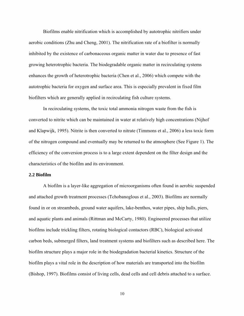
Biofilms enable nitrification which is accomplished by autotrophic nitrifiers under

aerobic conditions (Zhu and Cheng, 2001). The nitrification rate of a biofilter is normally

inhibited by the existence of carbonaceous organic matter in water due to presence of fast

growing heterotrophic bacteria. The biodegradable organic matter in recirculating systems

enhances the growth of heterotrophic bacteria (Chen et al., 2006) which compete with the

autotrophic bacteria for oxygen and surface area. This is especially prevalent in fixed film

biofilters which are generally applied in recirculating fish culture systems.

In recirculating systems, the toxic total ammonia nitrogen waste from the fish is

converted to nitrite which can be maintained in water at relatively high concentrations (Nijhof

and Klapwijk, 1995). Nitrite is then converted to nitrate (Timmons et al., 2006) a less toxic form

of the nitrogen compound and eventually may be returned to the atmosphere (See Figure 1). The

efficiency of the conversion process is to a large extent dependent on the filter design and the

characteristics of the biofilm and its environment.

2.2 Biofilm

A biofilm is a layer-like aggregation of microorganisms often found in aerobic suspended

and attached growth treatment processes (Tchobanoglous et al., 2003). Biofilms are normally

found in or on streambeds, ground water aquifers, lake-benthos, water pipes, ship hulls, piers,

and aquatic plants and animals (Rittman and McCarty, 1980). Engineered processes that utilize

biofilms include trickling filters, rotating biological contactors (RBC), biological activated

carbon beds, submerged filters, land treatment systems and biofilters such as described here. The

biofilm structure plays a major role in the biodegradation bacterial kinetics. Structure of the

biofilm plays a vital role in the description of how materials are transported into the biofilm

(Bishop, 1997). Biofilms consist of living cells, dead cells and cell debris attached to a surface.

11 

Accumulation of microorganisms at these interfaces has been described for every aqueous life

supporting system. Microbial structure of these communities ranges from a monolayer of

scattered single cells to thick, mucous structures of macroscopic dimensions consisting of

microbial mats and algal-microbial associations (Wimpenny et al., 2000). Factors that influence

the spatial structure of the biofilms include microcolonies, extracellular polymeric substances

(EPS), and channels.

Conclusive explanations for the structures observed in biofilms, requires the cooperation

of fields of investigation, mathematical modeling and experimental research (Wimpenny et al.,

2000). The use of current models applied to such complex cell structures in the biofilm assumes

that substrate nutrients diffuse from the bulk phase, through a liquid boundary layer at the

surface of the film to be utilized by the cells in the bacteria growth (Bishop and Kinner, 1986).

The expansion of molecular field techniques not only allows more and more detailed

documentation of the spatial distribution of species, but also of functional activities of single

cells in their environment of the biofilm.

Microbial cells growing on the filter media surfaces include nitrifying bacteria and

heterotrophs which are also sensitive to temperature and other water quality parameters. The

functional capability of the biofilter is dependent on the layer of biofilm which is near the surface

overlaid by nitrifying populations. However the outer layer of the biofilm is usually dominated

by heterotrophs in the presence of organic carbon which increases biofilm thickness (Malone and

Pfeiffer, 2006). Substrate bulk water concentration penetrates the biofilm layer dependent on the

water boundary layer prior to the biofilm (Tchobanoglous et al., 2003; Zhu and Chen, 2001) and

the thickness of the biofilm. The development of the biofilm layer which is based on the

reproduction rate of the bacteria that make up the layer is also temperature and substrate

12 

dependent. The temperature influence on biofilm growth process has influence on the ammonia

removal rates which are also related to the filter characteristics (Lyssenko and Wheaton, 2006) in

both suspended and attached growth systems.

2.3 Characteristics of Filters

Numerous variations in biofilter configurations have been used in semi-closed

recirculation systems. This is partly due to the fact that many individuals construct their own

biofilters, perhaps because of the same novelty which led people to the industry. In the

characterization of any nitrification system, the two most important physical characteristics of

biofilter media are a high surface area to volume ratio or specific surface area, and low clogging

(biofouling) properties (Wheaton et al., 1991). The latter is often strongly influenced by the

hydraulic characteristics of the particular biofilter as what may clog in one system may thrive in

another system. Characteristics of filters also include durability, availability, cost, and the often

related characteristics of specific gravity, weight, and buoyancy (Lawson, 1995).

However, the most common configurations designed include submerged, trickling,

rotating biological contactor (RBC), and fluidized bed biofilters (Lawson, 1995; Wheaton et al.,

1991; Timmons and Ebeling, 2007). Fluidized bed filters have a proven reputation for good

performance in aquaculture systems (Summerfelt, 2006; Timmons, et al., 2006), wastewater

(Tang et al., 1987), and solid waste land fill leachate systems (Martienssen et al., 1995; Kim et

al., 2006). Although fluidized bed sand filters have advantages which include high surface area,

non-clogging, high nitrification rates, high biomass concentrations, high hydraulic loading rates,

and close contact between the liquid and solid phase (Tang et al., 1987), fluidized bed sand

filters have their disadvantages too. Some of these include the difficulties in controlling of bed

expansion below wash-out or bed carry-over (Chang et al., 1991) and the requirement for high

13 

flow rates over the entire cross-section for fluidization (Wheaton et al., 1991). Therefore good

design is needed for effective biofiltration.

2.4 Fluidized Bed Flow

A number of different designs have been developed based on fluidized beds. One type of

flow distribution mechanism possibly developed specifically for applications in recirculating

aquaculture systems incorporated a pipe-manifold, originating at the top of the vessel, and then

distributing the flow into vertical pipes that extended down to the base of a sand bed (Weaver,

2006). The injection pipes were equally spaced across the filter with orifices in each tube for

uniform distribution of flow directly into the sand bed. However the emergence of different filter

designs including upflow and fluidized bed filters (Tchobanoglous et al., 2003) have

revolutionalized biofiltration processes in recirculation systems. Fluidized beds are an efficient,

relatively compact and cost-competitive technology for removing dissolved wastes from

recirculating aquaculture systems, especially in applications that require maintaining consistent

low levels of ammonia and nitrite (Summerfelt, 2006; Weaver, 2006).

Fluidized biofilters have been widely adopted in North America, especially in

recirculating systems that require excellent water quality to produce species such as salmon,

smolt, arctic char, rainbow trout, endangered fish and Ornamental or tropical fish (Weaver, 2006;

Summerfelt et al., 2004; Pfeiffer and Malone, 2006). Uniform flow distribution of water at the

base of the media bed (Figure 2) in a fluidized bed is critical for effective and reliable operation

(Summerfelt, 2006). There are various flow distribution mechanisms with at least five different

flow distribution mechanisms which have been used to uniformly inject water at the base of large

filters in recirculating aquaculture systems. A downward flow into the filter avoids penetration of

the vessel's walls with distribution pipes which also prevents the hydraulic head of water in the

14 

vessel from back flowing through the distribution piping when there is a check valve malfunction

(Summerfelt, 2006; Summerfelt et al., 2004). Single flow distribution filter systems consist of

either a media covered pipe-manifold or false-floor distribution chambers that sometimes are

used in relatively small recirculating systems (Summerfelt, 2006). In addition to the design

complexity, the media used in fluidized bed filters demands high flow rates needed for the filter

operation. The high flow rates required by fluidized bed filters may be the reduced in bead

filters.

Figure 2.1: Uniform flow distribution of water from base of media (U.S. Patent No. 5,232,586 by Ronald Malone, Department of Civil Engineering, Louisiana State University).

2.5 Bead Filters

Bead filters generally work in pressured vessels and use a media that is only slightly

buoyant (Timmons et al., 2006). Bead filters use polyethylene beads (Malone and Beecher,

2000) that are 2-3 mm in diameter. Specific surface area of beads typically used for the filtration

beds is 1150 – 1475 m2 m-3. The surface area per unit volume can be calculated based on the

15 

surface area of a sphere (4пr2) (Timmons et al., 2006; Greiner and Timmons, 1998). Surface area

and media porosity also enhance water flow characteristics of such filters. The bead filters are

mostly operated in the filtration mode.

In the operation mode water passes through the packed bead bed capturing solids 

(Pfeiffer et al., 2008) while enabling an active biofiltration process simultaneously. The volume

of water flowing through the media and the direction of flow is related to ammonia removal rates

of the filters (Zhu and Chen, 2001). Although increased flow could increase substrate utilization

rates, it also enhances solids capture and growth of heterotrophic bacteria on media which

requires cleaning (Backwash). Cleaning of the media bed is periodically required to release

excess biofloc and solids from the beads. The bioclarification and cleaning process is

accomplished by using a mechanical (Malone, 1992; Malone et al., 1993; DeLosReyes, 1997b)

pneumatic or hydraulic method (Malone, 1993; Pfeiffer et al., 2008). Although the filter serves

as a bioclarifier the biofilm that feed on carbon-nitrogen nutrient in the bulk water are cells that

exist in two forms in their biomass growth process: (a) suspended in solution as particulate

material and (b) fixed or attached to media (Tchobanoglous et al., 2003). The attached media is

the most popular form used in recirculating systems.

2.6 Attached Growth

Nitrification reactors based on bacterial films attached to fixed beds such as in trickling

filters and submerged filters, are generally attractive for treatment of water in intensive

recirculating aquaculture systems (Bovendeur et al., 1990). This is because high cell residence

times are maintained even when the hydraulic loading rates are high. The attached growth

biofilms are generally used for nitrogen removal because they allow longer biomass retention

time for reliable nitrification (Okabe et al., 1996). Microorganisms that make the film adhere to

16 

surfaces are of a broad population density while development of the biofilms that attach to the

surface is a net result of several physical, chemical and microbial processes. The processes

include the following: 1) transport of dissolved particulate matter from the bulk liquid to the

biofilm surface; 2) firm microbial cell attachment to the surface; 3) microbial transformations

(growth, reproduction, death etc.) within the biofilm and 4) partial detachment of biofilm due to

fluid shear stress (Characklis, 1981). A combination of the above describes biofilm

development as a growth process. Biofilm growth is also dependent on the configuration of the

reactors.

Fluidized biofilter configurations are the most common utilized by aquaculture system

managers (Wheaton et al., 1991). Fluidized bed filters have large surface area per unit volume

compared to other fixed film bioreactors. They therefore allow the capability of operation as a

plug flow at the liquid phase and mixed flow on the biological phase. As the concentration of

pollutant nutrient decreases in the aquatic systems, removal rate per surface area decreases. In

conventional bioreactors, the biological and liquid phases are mixed as in moving bed or plug

flow systems. In the moving bed system the filters operate at a minimum substrate concentration

(Sx), below this minimum concentration the bacteria cannot grow (Weaver, 2006; Zhu and Chen,

1999; Summerfelt, 2006). Although the fluidzed bed has the advantage of surface area, there are

disadvantages, which include control of bed expansion below wash-out or bed carryover (Chang

et al., 1991) stage. High flow rates required over the total surface area for the expansion may

wash some of the bacteria away which may affect the nitrification rate of the filter.

2.7 Nitrification

Nitrification was initially documented in waste water in 1887 (Peters and Foley, 1983).

Although nitrification is referred to as a two step biological process of converting ammonia

17 

(NH3) to nitrite (NO2) and nitrate (NO3-) through the action of autotrophic nitrifying bacteria.

The nitrification process is of great concern to commercial recirculating aquaculture systems

(Lawson, 1995; Boyd, 1990). This is due to the fact that efficiency of the nitrification process in

the biofilter influences the profit or loss in operation. Nitrification has been accomplished using

many technologies including sand and bead filters of different designs. The first step is

undertaken by bacterial populations which involve the oxidation of ammonia to nitrite by

ammonia-oxidizing bacteria (AOB) and the second step is subsequent oxidation of nitrite to

nitrate by nitrite oxidizing bacteria (NOB) (Kim et al., 2006).

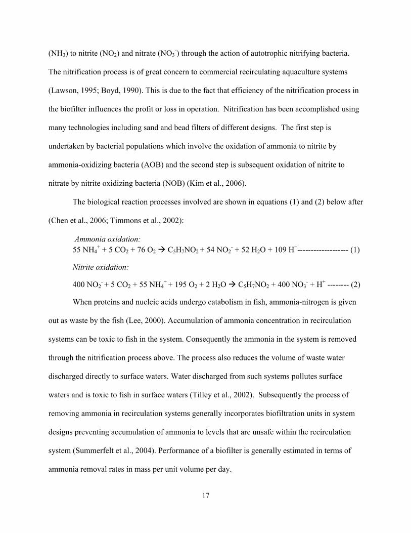
The biological reaction processes involved are shown in equations (1) and (2) below after

(Chen et al., 2006; Timmons et al., 2002):

Ammonia oxidation: 55 NH4

+ + 5 CO2 + 76 O2 C5H7NO2 + 54 NO2- + 52 H2O + 109 H+------------------- (1)

Nitrite oxidation:

400 NO2- + 5 CO2 + 55 NH4

+ + 195 O2 + 2 H2O C5H7NO2 + 400 NO3- + H+ -------- (2)

When proteins and nucleic acids undergo catabolism in fish, ammonia-nitrogen is given

out as waste by the fish (Lee, 2000). Accumulation of ammonia concentration in recirculation

systems can be toxic to fish in the system. Consequently the ammonia in the system is removed

through the nitrification process above. The process also reduces the volume of waste water

discharged directly to surface waters. Water discharged from such systems pollutes surface

waters and is toxic to fish in surface waters (Tilley et al., 2002). Subsequently the process of

removing ammonia in recirculation systems generally incorporates biofiltration units in system

designs preventing accumulation of ammonia to levels that are unsafe within the recirculation

system (Summerfelt et al., 2004). Performance of a biofilter is generally estimated in terms of

ammonia removal rates in mass per unit volume per day.

18 

2.8. Estimating Ammonia Removal Rates

Ammonia removal rates in biofiltration are determined from the kinetics of the processes

of converting ammonia to the intermediate product NO2-N and the final product NO3-N (Watten

et al., 2004). The rates of reactions are also influenced by the hydraulic characteristics of the

filter in terms flow (Watten et al., 2004; Malone et al., 2006). However the core theory of

reaction rate is rooted in Michaelis-Menton enzyme kinetics which is simply represented after

(Malone et al., 2006):

SK

SVRate

m max ------------------------------ (3)

Where Vmax is the maximum specific rate of substrate utilization (g day -1)

S is the substrate concentration (g m -3)

Km is the half saturation constant (g m -3)

However the equation is only applicable in conditions of constant enzyme availability (Malone et

al., 2006). When bioreactors exhibit dynamic bacterial growth, the reaction rates is expressed as:

bVSK

XSKRate

max ----------------------------- (4)

Where Kmax is the biomass normalized maximum rate constant in g of S converted per gram of biomass per day.

X is the bacterial biomass (g m-3)

Vb is the reactor volume (m3)

The actual reaction rates could also be affected by other factors including diffusion of substrate

into the biofilm, velocity of substrate flow over the surface of biofilm (Harremoes, 1982; Malone

and Beecher, 2000) and the kinetics of bacteria responsible for the nitrification process.

The Monod-type expression (Zhu and Chen, 2002, Zhu and Chen, 2001) for substrate removal

19 

rate further explains the bacterial kinetics in a biofiltration process expressed as:

)(max SKY

XSR

ss ------------------------------ (5)

Where R = Substrate removal rate (gm-3 d-1)

µmax = Specific growth rate (d-1)

X = Bacterial mass concentration (g cell m-3)

Ys = Yield of bacterial mass per unit of substrate used (g cell g-1 substrate)

S = Limiting-substrate concentration (g m-3)

Ks = Half saturation constant (g m-3)

This expression is substantiated by numerous studies and is considered a basic concept of

microbial kinetics. Although the Monod equation is empirical, it is basically identical to the

mechanistic model of the Michaelis-Menten equation, derived from the rates of chemical

reactions catalyzed by enzymes (Jorgensen and Halling-Sorensen, 1993; Malone et al., 2006). It

differs from the Michaelis-Menten equation by incorporating the bacterial biomass per substrate

concentration and yield of bacterial mass per unit of substrate used. Typical Michaelis-Menten

reaction kinetics is represented by the graph below (Figure 3). The models apply to typical

nitrification processes that occur in recirculating aquaculture systems (Zhu and Chen, 2002).

Biofilm kinetics is considered complex (Harresmoes, 1982) as the substrate supply within the

aggregate layer of bacterial film is affected by diffusion as well as the water boundary layer. In

addition there are also several other factors that influence nitrification rates.

20 

Figure 2.2- A Michaelis Menten graph of reaction kinetics (Recirculating Aquaculture Systems; Timmons et al., 2002; Timmons and Ebeling, 2007).

2.9 Factors Affecting Nitrification Rates

Removal of nitrogen from recirculating aquaculture systems considers the combination of

two competitive biological processes: autotrophic bacteria feeding on ammonia and

heterotrophic bacteria feeding on organic carbon (Ciudad et al., 2007). This is however affected

by many factors extraneous to the process, which include but are not limited to dissolved oxygen

(DO), pH, temperature, alkalinity, substrate concentration and biochemical oxygen demand

(BOD) (Zhu et al., 1999 and Ling and Chen, 2005). However the supply of oxygen in a

recirculating system is critical to maintain the nitrification process by bacteria.

2.9.1 Dissolved Oxygen

The supply of oxygen for the bacteria in the nitrification process is observed to be the

principal factor for the upper limit carrying capacity of filters (Manthe et al., 1988; Ling and

Chen, 2005). Oxygen concentrations must not fall below a limiting bulk water concentration

such as 2 mg liter-1 for submerged rock filters if complete nitrification is to occur (Manthe et al.,

1988). One of the major constraints of submerged biofilters is the limited supply of oxygen to

21 

support the nitrification process (Manthe et al., 1988; Manthe et al., 1984). The filter in a

nitrification process is normally assumed to have no internal source of oxygen. The oxygen flow

to the filter is therefore a function of the water flow rate to the media surface area. This

relationship can be expressed in terms of oxygen consumed by the filter:

OCF = Q*(Ci – Co) ---------------------------------------- (6)

Where OCF = Oxygen consumed in the filtration process (mg of O2 day-1; Q = flow rate through

filter (in liters day-1); Ci = filter influent oxygen concentration (in mg-O2 liter-1); Co = filter

effluent oxygen concentration (in mg-O2 liter-1). The OCF also reflects the amount of oxygen

consumed in the filter due to instantaneous impact of biochemical oxygen demand and the

respiration of the bacteria (Manthe et al., 1988).

Assuming a minimum oxygen concentration of 2.0 mg liter-1 is required to avert inhibition of

bacteria in the filter. The oxygen carrying capacity of the filter is expressed as:

OCC = Q*(Ci –2.0) -------------------------------------------- (7)

Where OCC = oxygen carrying capacity of filter (in mg-O2 liter-1). It is therefore necessary to

have the oxygen flow in the system above the minimum required concentration for removal of

ammonia.

2.9.2 Total Ammonia Nitrogen (TAN)

The concentration of total ammonia nitrogen (TAN) substrate in the nitrification process

is also an important factor to consider in the design and operation of biofilters (Chen et al.,

2006). Nitrification reaction which occurs in the biofilm by utilizing ammonia substrate depends

on the local substrate concentration in the biofilm (Zhu and Chen, 2002). The nitrifying

populations are therefore substrate limited in the nitrification process by the concentration of

substrate available to the bacteria population deep within and at the surface of the biofilm (Horn,

22 

1994; Rasmussen and Lewandowski, 1998; Zhu and Chen, 1999). Ammonia concentrations

falling below the limiting substrate concentrations may impair the nitrification process while

excessive substrate concentration affects the ratio of food to microorganism (F/M). Subsequently

the nitrification process is independent of the concentration when there is high F/M ratio

(Tchobanoglous et al., 2003; Tchobanoglous et al., 1991). Although the nitrification process

occurs above limiting substrate concentration, it is also influenced by pH of the system.

2.9.3 Effects of pH on Nitrification

The reported pH range for optimum nitrification is 7.0 to 8.8 (Antoniou et al., 1990; Chen

et al., 2006). The optimal range is determined by three effects the pH exerts on the nitrifying

bacteria, a) Activation – deactivation of nitrifying bacteria, b) Nutritional effect associated with

alkalinity and c) Inhibition through free ammonia and free nitrous acid (Villaverde et al., 1997).

The nitrification process consumes alkalinity (HCO3-) and produces carbonic acid (H2CO3).

Changes in alkalinity due to HCO3- consumption lowers water resistance while the carbonic acid

lowers the pH. The pH drop in aquaculture applications is normally due to CO2 accumulation

(Loyless and Malone, 1997). A possible cause of such change is due to poor or inadequate

aeration and degassing. Free ammonia concentration depends heavily on pH based on the

following equation:

pHwa

pH

free KK

NNHNNH

10/

10*][][ 4

3

--------------------------- (8)

The hydrolysis of ammonia reaction constant is dependent on temperature:

Ka/Kw = exp[6334/(273 + T)] ----------------------------------- (9)

The variation of pH is to a large extent associated with poor aeration of the system, which

implies aeration is considered an integral part of the system dynamics in the entire nitrification

23 

process. Proper pH management is required for obtaining optimum performance for recirculating

systems (Loyless and Malone, 1997), for CO2 control and alkalinity adjustments.

2.9.4 Alkalinity

The conversion of ammonia to nitrate consumes alkalinity in the form of bicarbonate

supplement. Alkalinity in the form of carbonate and bicarbonate becomes the nutrient element

for nitrifying bacteria (Chen et al., 2006). Alkalinity is normally consumed at approximately

7.14 g/g Noxidized during nitrification (Timmons et al., 2002). It should be emphasized that pH

dependent equilibrium exists between carbon dioxide (CO2) and alkalinity to maintain

concentrations of CO2 below the animal stress level of 15 mg/l. The equilibrium prevents

potential ion imbalance. It is recommended that a maximum alkalinity concentration of 200 mg/l

as CaCO3 for nitrification in fresh warm water (< 10 ppt salinity) recirculating aquaculture

systems be used for the pH range 7.5 to 8.0 (Loyless and Malone, 1997). The interdependence

between the two can be used to adjust pH physically through the (HCO3-) contents of the water

or chemically adjusting the alkalinity. A greater alkalinity presents a higher nitrification process

(alkalinity consumption) while nitrification increases linearly with increase in alkalinity (Chen et

al., 2006). However, maintaining the alkalinity level for optimal nitrification may be undermined

by the presence of excessive organic material, which encourages growth of heterotrophic

bacteria.

2.9.5 Organic Loading

The ratio of organic carbon and inorganic nitrogen (C/N) in water connects the

availability of growth area per media and competition for organic carbon and ammonia (Michaud

et al., 2006). Although the impact of organic matter on nitrification has attracted increasing

research attention recently, however quantitative information regarding the degree of impact on

24 

biofliters in aquaculture is still being studied (Zhu and Chen, 2001). A decrease in nitrification is

generally associated with increased organic loading (Bovendeur et al., 1990) due to the fact that

the biodegradable organic matter in recirculating aquaculture systems generally supports growth

of heterotrophic bacteria which compete with the autotrophic nitrifiers, especially in fixed film

bioreactors (Zhu and Chen, 2001).

The inhibition of nitrification efficiency due to the presence of organic carbon is called

allelopathy (Michaud et al., 2006). Inhibition of the nitrification process in the presence of

organic carbon is partly attributed to the increase in the growth of the heterotrophs consuming

oxygen which subsequently reduces dissolved oxygen concentration in the biofilm for the

nitrifying bacteria (Chen et al., 2006; Satoh et al., 2000). This effect is also due to the faster

growth rate heterotrophic bacteria which finally outgrow nitrifiers, subsequently reducing

substrate penetration of the biofilm. Finally temperature changes warming the system associated

with growth favors faster growth of most microorganisms (heterotrophic & other bacteria)

(Malone and Pfeiffer, 2006).

2.9.6 Temperature

Recirculating aquaculture systems are controlled by system managers. However in

several recirculation systems, water temperature fluctuates based on exposure to environmental

or other factors. Temperature change influences the metabolic processes of fish in the system

producing ammonia with increasing fish size (Tseng and Wu, 2004). Temperature also

influences bacterial kinetics of the nitrification process in the biofilter operation. Bacterial

reaction rates tend to increase with rising temperatures for suspended film filtration systems

while no significant effect has been acknowledged for fixed film series bioreactors (Zhu and

Chen, 2002; Zhu and Chen, 1999). However, nitrification with biodrums and landfill leachate

25 

studies indicated an increased nitrification effect with increase in temperature (Wortman and

Wheaton, 1991; Kim et al., 2006). Impact of temperature on fixed film filtration systems is still

widely studied (Pedersen et al., 2007) because of the complexity of the bacteria kinetics involved

(Harresmoes, 1982) in the nitrification process. Bacterial reaction nitrification kinetics have been

described with respect to temperature using the Van’t Hoff-Arrhenius equation which provides a

general estimate of reaction rates expressed as:

µmax = µ20 θT-20 ----------------------------------------------- (10)

Where µmax=Specific growth rate (d-1)

µ20 = the value of µ at 200C (d-1)

θ = temperature coefficient (Dimensionless)

T = Temperature in 0C

Expanding the Monod equation (5) for the bacterial reaction rate in the nitrification process is

expressed after (Zhu and Chen, 2002) as:

)(

2020 SK

S

Y

XR

s

T

---------------------------------- (11)

Where X is mass concentration (g cell m-3), Ys is yield of bacterial mass per unit of substrate

used (g cell g-1 substrate), S is limiting-substrate concentration (g m-3), Ks is half saturation

constant (g m-3)

The effect of temperature on the nitrification process is an area of interest in ongoing

research with diverse opinions on the temperature–biofilm interactions. In the ever increasing

demand for fish protein, the focus of system managers has shifted to optimization of system

26 

productivity while reducing cost of operations (Malone and Beecher, 2000) including improving

biofilter performance. These important components of recirculating systems perform complex

bacterial biofiltration at varying temperature regimes depending on the location of the system

and the temperature of the surroundings. It is therefore noteworthy to further investigate transient

(short term) temperature effects on nitrification at steady state and diurnal temperature (daily or

possible long term) variation.

Numerous studies of temperature interaction with biofiltration, specifically removal of

total ammonia nitrogen (TAN) in recirculation systems have been devoted to optimizing biofilter

performance at steady state temperatures. However apart from those factors mentioned above,

other factors such as temperature variations for seasonal cold fronts, daily diurnal temperature

variations and media acclimation at steady state temperature while exposed to diurnal regimes;

could also affect the ammonia removal rate in the biofiltration process. This dissertation also

calls attention on the importance of the cumulative effects arising from daily diurnal temperature

variations in the nitrification process. This section also points out where and how this research

differs from previous studies and the importance of modeling for standardizing biofilter

performance for the future.

Earlier studies in the area of biofiltration focused on understanding the kinetics of

biofiltration (Harresmoes, 1982). Since then more biofiltration studies have been done in areas of

design characteristics (Malone and Beecher, 2000) and enhancing performance (Wortman and

Wheaton, 1991; Zhu and Chen, 2002; Malone et al., 2006). In contrast to the extensive studies

done in biofiltration, similar work has been limited to enhancing performance of the biofilter at

steady state temperatures. Two main groups of researchers have looked at temperature effect on

biofiltration. Zhu and Chen (2002) could not find any significant effect of temperature on

27 

biofiltration performance within a range of 14 - 27oC. Wortman and Wheaton (1991) found a

linear effect of temperature on biofiltration performance across a broader range 7- 35oC. All

other studies have been supportive of a linear or non linear relationship between temperature and

biofilter performance.

A limited number of studies are known to have contributed to the temperature

performance relationship. However little is known of short term temperature effects on

biofiltration especially in the acclimation and seeded stage of operations. One of the major

factors in managing recirculation systems is the environmental temperature the system is

exposed to during operation. Temperature of the environment is not necessarily steady as

presumed in most of these studies. In fact exposure to temperature variations in uncontrolled

facilities is subject to daily diurnal temperature variation. Finally media acclimation done

indoors at a controlled temperature and utilized in outdoor systems prior to a steady biofilm may

be subject to temperature acclimation changes in performance, continued bacterial growth in

addition to daily diurnal temperature variations. These factors have not been adequately

addressed in other studies.

2.10 References

Bishop, P.L., 1997. Biofilm structure and kinetics. Wat. Sci. Tech., Vol. 36, No. 1, pp 287-294. Bishop, P., Kinner, N., 1986. Aerobic fixed-film bioprocesses. In: Biotechnology, VCH

verlagsgellschaft, Weinheim, Germany, pp 113 – 176. Boyd, C. E., 1990. Water Quality in Ponds for Aquaculture; Alabama Agricultural Experiment

Station: Auburn University, AL. Bovendeur, J., Zwaga, A. B., Lobee, G. J., Blom, H. J., 1990. Fixed-Biofilm Reactors in

Aquacultural water recycle systems: Effects of Organic Matter Elimination on Nitrification Kinetics, Wat. Res., Vol. 24, No. 2, pp. 207 – 213.

28 

Characklis, W.G., 1981. Fouling biofilm development a process analysis, Biotechnology and Bioengineering, Vol. XXIII, Pp 1923-1960.

Chang, H. T., Rittmann, B. E., Amar, D., Heim, R., Ehlinger, O., Lesty, Y., 1991. Biofilm

detachment mechanism in a liquid fluidized-bed. Biotechnology and Bioengineering. 38 pp 499-506.

Chen, S., Ling, J., Blancheton, J., 2006. Nitrification kinetics of biofilm as affected by water quality factors. Aquacultural Engineering. 34, 179-197.

Ciudad, G. González, R. Bornhardt, C., Antileo, C., 2007. Modes of operation and pH control as enhancement factors for partial nitrification with oxygen transport limitation Water Research, Volume 41, Issue 20, Pages 4621-4629.

Davidson, J., Helwig, N., Summerfelt, S.T., 2008. Fluidized sand biofilters used to remove

ammonia, biochemical oxygen demand, total coliform bacteria, and suspended solid from an intensive aquaculture effluent. Aquacultural Engineering,Volume 39, Issue 1, Pages 6-15

DeLosReyes, A.A. Jr.,Rusch, K.A., Malone, R.F., 1997b. Performance of commercial scale

recirculating alligator production system employing a paddle-wash floating bead filter. Aquacultural Engineering, 16, 239-251.

Gutierrez-Wing, M., Malone R.F., 2006. Biological filters in aquaculture: Trends and research

directions for freshwater and marine applications. Aquacultural Engineering, Volume 34, Issue 3, Pages 163-171

Harresmoes, P., 1982. Criteria for nitrification in fixed film reactors. Water Sci. Technolo. 14,

167-187.

Horn, H., 1994. Dynamics of a nitrifying bacteria population in a biofilm controlled by an oxygen microelectrode. Water Sci. Technol. 29, 69.

Jorgensen, S. E., Halling-Sorensen, B., 1993. “Nitrogen compounds as pollutants.” in The

Removal of Nitrogen Compounds from Wastewater, Elsivier Science Publishers: B. V., Amsterdam, The Netherlands; pp 3-40.

Kim, D., Lee, D., Keller, J., 2006. Effects of temperature and free ammonia on nitrification and

nitrite accumulation in landfill leachate and analysis of its nitrifying bacterial community by FISH. BiosourceTechnology., 97, 459-468.

29 

Lawson, T. B., 1995. Fundamentals of Aquacultural Engineering; Chapman and Hall Publishers: New York.

Lawson, T.B., Drapcho, C..M., McNanama, S, Braud, H. J. 1989. A heat Exchanger system for Spawning red drum. Aquacultural Engineering 8, pages 177-191 Lee, P. G., 2000. Process control and artificial intelligence software for aquaculture.

Aquacultural Engineering, 23, 13-36. Ling, J., Chen, S., 2005. Impact of organic carbon on nitrification performance of different

biofilters, Aquacultural Engineering, Volume 33, Issue 2, Pages 150-162. Loyless, J.C., Malone, R. F., 1997. A sodium bicarbonate dosing methodology for pH

management in freshwater-recirculating aquaculture systems. The progressive fish Culturist, 59: 198-205.

Malone R.F., Chitta, B.S., Drennan , D.G., 1993. Optimizing Nitrification in bead filters for

warm water recirculating aquaculture systems. In: Jaw- Kai Wang (Ed.), Techniques for Modern Aquaculture. ASAE Publication 02-93 (ISBN 0-9293355-40-7; LCCN 93-71584).

Malone, R. F., Pfeiffer, T. J., 2006. Rating fixed film nitrifying biofilters used in

recirculating Aquaculture systems. Aquacultural Engineering, Volume 34, Issue 3, Pages 389-402.

Malone. R. F., Beecher, L. E., 2000.Use of floating bead filters to recondition recirculating waters in warmwater aquaculture production system. Aquacultural Engineering, Volume 22, Issues 1-2, May 2000, Pages 57-73.

Malone, R. F., Bergeron, J., Chad, C. M., 2006. Linear versus monod representation of ammonia

oxidation rates in oligotrophic recicrculating aquacultutre system. Aquacultural Engineering, Volume 22, Issues 1-2, May 2000, Pages 57-73.

Malone, R.F., 1993. Floating media hour glass biofilter. United States Patent Number 5,232,586. August 3.

Malone R.F., 1992. Floating Media biofilter. United State Patent Number 5,126,042. June 30. 

Manthe, D. P., Malone, R. F., Kumar, S., 1988. Submerged rock filter evaluation using an oxygen consumption criterion for closed recirculation systems, Aquacultural Engineering, 7, 97 – 111.

30 

Manthe, D. P., Malone, R. F., Kumar, S., 1984.Limiting factor associated with nitrification in closed blue crab shedding systems., Aquacultural Engineering, 34, pages 332 – 343.

Martienssen, M., Schulze, R., Simon, J., 1995. Capacities and limits of three different

technologies for the biological treatment of leachate from solid waste landfill sites. Acta Biotechnology. 15, pp. 269–276.

Michaud, L., Blancheton, J.P., Bruni, V., Peidrahita, R., 2006. Effects of particulate organic carbon on heterotrophic bacterial populations and nitrification efficiency in biological filters, Aquacultural Engineering 34, 224-233.

Nijhof, M., Klapwijk, A., 1995. Diffusional transport mechanisms and biofilm nitrification

characteristics influencing nitrite levels in nitrifying trickling filter effluents, Wat. Res. Vol. 29, No. 10. pp 2287-2292.

Okabe, S., Oozawa, Y., Hirata, K., Wantanabe, Y., 1996. Relationship between population

dynamics and nitrfiers in biofilms and reactor performance at various C:N ratios, Water Research, Volume 30, Issue 7, Pages 1563-1572.

Pedersen, L., Pedersen, P.B., Sortkjær, O., 2007. Temperature-dependent and surface specific

formaldehyde degradation in submerged biofilters. Aquacultural Engineering, Volume 36, 2, Pages 127-136

Peters, R. W., Foley, V. L., 1983. “Fixed-film wastewater treatment systems: Their history

and development as influenced by medical, economic, and engineering factors.” in Wu, Y. C. and E. D. Smith (Ed.) Fixed-Film Biological Processes for Wastewater Treatment; Noyes Data Corporation: Park Ridge, New Jersey, pp 1-51.

Pfeiffer, T. J., Osborn, A. Davis, M., 2008. Particle sieve analysis for determining solid removal

efficiency of water treatment components in a recirculating aquaculture system. Aquacultural Engineering, Volume 39, Issue 1, Pages 24-29.

Rasmussen, K., Lewandowski, Z., 1998. Microelectrode measurements of local mass transport

rates in heterogeneous biofilms . Bioeng. 59, 302. Rittman, B. E., McCarty, P. L., 1980. Model of steady state biofilm kinetics, Biotechnology and

Bioengineering, Vol XXII, Pp 2343-2357. Satoh, H., Okabe, S., Norimatsu, N., Watanabe, Y., 2000. Significance of substrate C/N ratio on

structure and activity of nitrifying biofilms determined by in situ hybridization and use of microelectrodes. Water Sci. Technol. 41 (4-5), 317-321.

31 

Summerfelt, S.T., Wilton, G., Roberts D., Rima, T., Fonkalsrud, K., 2004. Developments in recirculating systems for artic char culture in North America. Aquacultural Engineering, 30, pp 31-71.

Summerfelt, S.T., 2006. Design and management of conventional fluidized sand biofilters,

Aquacultural Eng. 34 (3), pp 275-302. Tang, W. T., Wisecarver, K., Fan, L. S., 1987. Dynamics of a draft tube gas—liquid—solid

fluidized bed bioreactor for phenol degradation. Chemical Engineering Science, Volume 42, Issue 9, Pages 2123-2134.

Tchobanaglous, G., Burton, F., 1991. Wastewater Engineering Treatment, Disposal and Reuse,

3rd ed. McGraw-Hill, New York, P.1334 Tchobanaglous, G., Burton, F., 2003. Wastewater Engineering Treatment, Disposal and Reuse,

4th ed. McGraw-Hill, New York. Tilley, D. R., Badrinarayanan, H., Rosati, R., Son, J., 2002. Construction wetlands as

recirculation filters in large-scale shrimp aquaculture. Aquacultural Engineering, 26, pp 81-109.

Timmons, M. B., Holder, J. L., Ebeling, J. M., 2006. Application of microbead biological filters. Aquacultural Engineering, Volume 34, Issue 3, Pages 332-343.

Timmons, M. B., Ebeling, J. M., Wheaton, F.W., Summerfelt, S. T., Vinci, B.J., 2002.

Recirculating aquaculture systems 2nd Ed Tseng, K., Wu, K., 2004. The Ammonia removal cycle for a submerged biofilter used in a

recirculating eel culture system. Aquacultural Engineering. 31, 17-30. Villaverde, S., Garcia-Encina, P. A., FDZ-Polanco, F., 1997. Influence of pH over nitrifying

biofilm activity in submerged biofilters, Wat Res., Vol 31, No. 5, pp 1180 – 1186. Watten, B.J., Sibrell, P.L., Montgomery, G.A., Tsukuda, S. M., 2004. Modification of pure

oxygen absorption equipment for concurrent stripping of carbon dioxide. Aquacultural Engineering, Vol. 32, pp 183-208.

Weaver, D. E., 2006. Design and operations of fine media fluidized bed biofilters for meeting

oligotrophic water requirements. Aquacultural Engineering., Volume 34, Issue 3, pages 303 – 310.

32 

Wheaton, F. W., Hochheimer, J. N., Kaiser, G.E., Krones, M.J., 1991. “Priciniples of Biological Filtration” in Northeast Regional Aquacultural Engineering Service. Engineering aspects of intensive aquaculture. Procedings from aquaculture symposium. New York: Cornell University. 1991: 1-31.

Wimpenny, J., Manz, W., Szewzyk, U., 2000. Heterogeneity in biofilms. FEMS Microbiology Reviews, 24, Issue 5, Pages 661-671.

Wortman, B., Wheaton, F., 1991., Temperature effects on biodrum nitrification. Aquacultural. Engineering, 10, pp. 183-205. Zhu, S., Saucier, B., Durfey, J., Chen, S., Dewey, B., 1999. Waste excretion characteristics

of Manila clams (Tapes philippinarum) under different temperature conditions Aquacultural Engineering, Volume 20, Issue 4, Pages 231-244.

Zhu, S., Chen, S., 2002. Impact of temperature on nitrification rate in fixed film biofilters. Aquacultural Engineering, 26, 221 – 237.

Zhu, S., Chen, S., 2001. Effects of organic carbon on nitrification rate in fixed film biofilters,

Aquacultural Engneering, 25, p1-11. Zhu, S., Chen, S., 1999. An experimental study on nitrification biofilm performances using a

series reactor system. Aquacultural Engineering, 20, pp245 –259. Zhu, S., Chen, S., 2001. Impacts of Reynolds number on nitrification biofilm kinetics,

Aquacultural Engineering, 24, 213-229.

33 

Chapter 3- Temperature Effect on Biofilter Total Ammonia Nitrogen Removal Rate Performance

3.1 Introduction

Biofilter performance is one of the most important aspects of recirculating aquaculture

systems in controlled fishery production. Fishery product consumption per capita increased in

the US by nearly 30% over the last two decades, with aquaculture accounting for 11% of the

seafood consumed (Wortman and Wheaton, 1991; USDA, 2008). Although seafood supply from

captured fisheries grew at annual average rate of 1.2%, aquaculture supply grew at a rate of 9.1%

(Gutierrez-Wing and Malone, 2006). The increase in supply is due to growing consumer demand

for sea food which has further encouraged import of sea food to the United States to supplement

production from traditional fishing and aquaculture systems (USDA, 2008).

However systems are challenged with constraints including water shortages, discharge

regulations, demand for high quality product, coastal land use, and decreasing water quality in

natural waters (Zhu and Chen, 2002). Recirculating aquaculture systems are a possible solution

to the demand and challenges of traditional aquaculture (Wortman and Wheaton, 1991; Malone

and Beecher, 2000; Ayer and Tyedmers, 2009). It is therefore no surprise that recirculating

systems are gaining popularity for use in effectively managing removal of waste and pollutants

where water quality and disease issues dominate (Davidson et al., 2009). Typical applications of

recirculating systems are for conditioning of marine brood stock, production of larvae, fry and

fingerlings for grow-out systems (Malone et al., 2006, Malone 2002).

Recirculating aquaculture systems are designed to accommodate the cultured organism

and to maximize production. Although the design and increased adoption of recirculating

systems appear to have stemmed from the need for precise control of temperature and light,

34 

utilization of recirculating systems is now mostly driven by the desire to control water quality,

disease and nutritional conditions in the systems (Malone et al., 2006).

Recirculating aquaculture systems are well established in aquaculture, with capability of

performing essential mechanical, chemical and biological processes to ensure quality aquaculture

products (Watson and Hill, 2006). The biological process is a key aspect of recirculating

systems criteria in addition to aeration, clarification, solids capture and circulation, impacted by

system management and control (Malone and Beecher, 2000). A biological filtration process

consumes toxic soluble waste (ammonia) produced in recirculation systems (Nijhof and

Klapwijk, 1995; Timmons et al., 2006). This process is critical to improving the cost

effectiveness and productivity of recirculating aquaculture systems if they are to compete

directly with other production methods including net pens and open pond systems (Malone and

Beecher, 2000; Wortman and Wheaton, 1991; Lyssenko and Wheaton, 2006).

The biofiltration process is influenced by several factors such as pH, alkalinity, ammonia

concentration, oxygen, salinity, organic loading and temperature (Tseng and Wu, 2004; Hao and

Huang, 1996; Groeneweg et al., 1994). In a recirculating system the control of temperature for

organisms raised also impacts the bacteria reaction rates in the biofiltration process. The

temperature impact related to the removal of toxic ammonia in the system is a major parameter

in biofilter performance (Wortman and Wheaton, 1991; Watson and Hill, 2006).

An approach to examine short-term temperature impact on biofiltration performance while

understanding the ramifications on acclimation of biofilters will contribute to possible best

management practices to commercial recirculating aquaculture producers.

3.2 Background

Biofilters are designed based on their capacity to utilize ammonia (in grams) per cubic meter of

35 

media volume per day (g/m3/d) or milligrams per square meter of media surface area per day

(mg/m2/day) in a biofiltration process (Silapakul et al., 2005; Malone et al., 2006). The rate of

utilizing ammonia in the biofilm is an equilibrium process between the demand for substrate

from bacterial biomass growth and the rate of substrate supply. The substrate supply is

influenced by diffusion transport limitations (Rasmussen and Lewandowski, 1998; Chen et at.,

2006). However factors that affect substrate diffusion and bacterial growth also influence the

nitrification process and bacterial reaction rate (Chen et al., 2006).

Previous studies and theoretical principles have been core to determining influence of

temperature in the design and operation of biological reaction filters (Zhu and Chen, 2002;

Wortman and Wheaton, 1991). General predictions of the relationship between temperature and

suspended bacteria reaction rates, follows a Van’t Hoff Arrhenius curve (Zhu and Chen, 2002;

Tchobanoglous et al., 2003). It is also indicated in previous studies that increasing temperature

for bacterial reactions above an optimal value can disable enzymes on denature protein (Sawyer

et al., 1994; Zhu and Chen, 2002; Tchobanoglous et al., 2003). A representation of the general

estimate of temperature effect on biological reaction rates is indicated by the expression

(Tchobanoglous and Burton, 1991) below:

2020

T -------------------------------- (12)

Where μ is the rate coefficient (d-1), μ20 is the value of μ at 20oC (d-1), θ is temperature

coefficient dimensionless and T is temperature (oC). However, short term temperature impact on

biofilter performance has not been examined in detail for fixed film and dynamic growth biofilter

systems (Wheaton et al., 1994).

Temperature variation of biofilters in recirculating aquaculture systems during each 24 hr

cycle may also vary, inducing a 24 hr cyclic diurnal temperature pattern in biofilters exposed to

36 

outdoor or intermediate environmental fluctuating temperature regimes. Determining the effect

of such temperature variations on biofilters in relation to total ammonia nitrogen (TAN)

utilization may be essential for design and performance of biofilters in recirculating systems.

Ammonia utilization in biofiltration systems can be divided into three stages (Zhang and

Bishop, 1994; Harremoes, 1982; Hagopian and Riley, 1998), with the first involving the

substrate diffusion through the fluid boundary layer leading to the biofilm. The second stage

involves substrate diffusion through the biofilm to the bacteria. The final stage involves nutrient

availability to the bacteria within the biofilm. These stages are generally incorporated into

reaction kinetic models to adequately describe the biofiltration process. Monod models that are

used to represent fixed film nitrification kinetics in biofilters indicate the complexity of transport

and enzyme reactions (Malone et al., 2006; Bishop, 1997; Golz et al., 1999). The stages of the

reaction and enzyme kinetics that occur are simply represented by the Michaelis-Menton

expression which is used to represent fixed film nitrification kinetics (Knowles et al., 1965; Zhu

and Chen, 2002):

SK

SVR

m max ------------------------------------- (13)

Where R is the substrate removal rate (g m3 day-1), Vmax is the maximum specific rate of substrate

utilization (g day-1); S is the substrate concentration (g m-3); and Km is the half saturation

constant (g m-3). Equation (13) above is applicable to systems with controlled biomass. However

when the equation is applied to more dynamic bacterial growth systems, it is expressed by the

Monod formulation:

SK

S

Y

XR

mm max

--------------------------- (14)

37 

Where μmax is maximum specific growth rate (day-1), X is the bacterial biomass concentration (g

cell m-3), R is the substrate removal rate (g m-3 day-1) Ym is the yield of bacterial mass per unit of

substrate used (g cell g-1 of substrate) and Km is the half saturation constant.

The volumetric TAN removal rate is similarly modeled as:

SK

SVtrVtrVR

mb

max/ ---------------------------- (15)

Where Vtr (g m-3 day-1) is the TAN conversion rate, Vtrmax (g m-3 day-1) is the maximum Vtr that

can be attained and Vb is the filter volume. An in-depth understanding of the biofilter TAN

removal rate performance in relation to temperature interaction with nitrification process could

contribute to the much needed improvement in biofilter performance, management practices and

cost effective production of recirculation systems. The objectives of this study were to examine

short term temperature impact on biofilter performance at steady state, diurnal and step

temperature regimes. Setting up the experiments required development of custom designed

laboratory temperature controlled tank systems while using laboratory sampling procedures that

are applicable universally.

3.3 Materials and Methods

A batch bioreactor system of tanks with intake airlift pumps attached for continuous

water flow and aeration of the reactors was designed and developed for this study. The system

consisted of 36 tanks, 9 were used to perform the 3 X 3 experiments. Enhanced nitrification

polyethylene media (EN-Media manufactured by Aquaculture Systems Technologies, LLC-New

Orleans, LA) beads with a diameter of ≈ 3 mm (Figure 3.1) were used for bacterial growth for

reactors in the tanks. The total biofilm surface area was assumed to include the media surface

area and the inner walls of the bead contact area (Appendix E) in the reactor, while the

38 

calculated volume was based on the dimensions of the media water volume of biofilter.

All tanks were 40 L in volume. Each reactor had approximately 24 recirculating passes

per tank volume per day. Synthetic substrate consisting of ammonium chloride (NH4Cl) and

other trace nutrients (Table 3.1) suitable for ammonia oxidizing bacteria (AOB) growth was

mixed in a separate tank (Figure 3.2), and pumped into the individual tanks containing the

reactors. The reactor volume (4 x 10-4 m-3) was calculated (Appendix E) at the construction

stage. Bacteria growth on reactor media was induced by inoculating with seed bacteria from an

existing aquarium. The inoculated tank was loaded with synthetic substrate from the general

mixing tank at 5 g m-3 ammonia nitrogen concentration for bacteria growth and consistency in

concentration. Inoculation and bacteria growth lasted from 3-8 weeks. The acrylic bioreactors

were centered 0.15 m (6″) from one end of the tank (Figure 3.3).

The biofilters were designed using an acrylic tube with the following dimensions.

1. The height of filter is 19.1 cm (7.5″)

2. Internal diameter is 5.1 cm (2″)

3. The base/stand dimension is 5.1 x 5.1 cm (4″ x 4″)

4. Inflow screen porosity is 2 mm x 3 mm = 6 x 106 μm2

5. Outflow screen porosity is 2 mm x 3 mm = 6 x 106 μm2

6. Bead loading depth in filter 6.4 cm (2.5″)

The bacterial growth stage was considered complete when a steady removal rate was achieved

for samples, but later analyses of the data indicated that the bacterial mass was still in the growth

phase. The temperature of the acclimation growth stage was set at 25oC which was considered to

be optimal for growth of nitrifying bacteria (Lyssenko and Wheaton, 2006) and pH was

maintained at 7.0 - 8.6 (Hagopian and Riley, 1998, Wheaton et al., 1994).

39 

 

 

Figure 3.1: Enhanced nitrification media in the bacteria culture tank.

 

Figure 3.2: Fiberglass nutrient mixing tank (0.91 m in diameter- Total volume ≈ 500 L).

Enhanced Nitrification (EN) Media

91.4 cm

3 mm

40 

 

Figure 3.3: Biofilter at one end of tank with airlift for water circulation.

Table 3.1: Chemical composition of substrate nutrients: (Wortman and Wheaton, 1991).

Compound Source Concentration (mg/liter) ______________________________________________________________________________ NaHCO3 Louisiana State University Store/VWR.com 100 K2HPO4 ″ 15 CaCl2 ″ 15 NH4Cl ″ 5 (as N) MgSO47H2O ″ 100 FeCl36H2O ″ 5  

Dissolved oxygen was maintained above 6 g m-3 considered to be above limiting concentration

levels (Zhu and Chen, 2002; Zhu and Chen, 1999). Beads in the biofilters were acclimated prior

to experimental sampling.

3.3.1 Biofilter Bead Acclimation

EN-Media used in the bacterial inoculation and growth stage were used for loading the acrylic

5.08 cm

Flow direction 

2.54 cm

41 

biofilter columns with attached PVC airlifts. This ensured that the beads were from the same

pool (inoculation tank) under same growth conditions. Media beads were acclimated at three

steady state temperatures (13, 20 & 30oC), and mixed after the 3 d steady state experiments in a

common container. The mixed beads were loaded into separate biofilters and subjected to the

diurnal temperature (20 ± 30C and 30 ± 30C) regimes.

All cylindrical filter columns were loaded with beads to a depth of 2.5 in (6.4 cm). The

unit biofilters were submerged into nine independent 40 L tanks loaded with nutrient solution.

The independent tanks (Figure 3.4) were randomized for triplicates at each temperature regimes

using a computer automated control system. The tanks were acclimated at the temperature

regimes settings for 3 consecutive days before starting experimental sampling. The tanks

containing loaded bead reactors were sampled after acclimation, and each reactor started at a

fixed concentration (5 g m-3) after acclimation.

3.3.2 System Sanitization

The acrylic reactor cylinders were sanitized between runs to minimize in-situ-nitrification

which had proven to be problematic in previous studies (Malone and Beecher, 2006; Malone et

al., 2006). After each set of experiments the beads were taken out of the reactor and set aside in

individual 20 L containers for 2 h to maintain consistency of the biofilms during the sanitization

stage. The reactors were then washed with diluted 1250 parts per million (ppm) bleach (chlorine)

water, with all the pieces taken apart, scrubbed out and dropped into the tanks for bleach water

circulation in the tank. Tanks were each loaded with 50 ml of concentrated bleach (Clorox

purchase from Walmart) per 40 L tank achieving a concentration of 1250 parts per million (ppm)

of bleach per liter of water in each tank. The chilling pumps were activated to circulate the

diluted bleach within the tank and through the heat exchangers which had the potential of

42 

bacterial growth on the inside. The system was allowed to run for 2 hr, after which the tanks

were drained using electric motor operated suction pumps.

The reactors were rinsed with deionized distilled water. The tanks were flushed with tap

water (chlorine < 0.2 ppm) using the same chilling pump activation setup. This ensured that the

residual bleach water in the heat exchangers was also flushed out. The system was drained for a

second time to be reloaded with synthetic substrate for the next experimental setup. The reactors

were taken out of the drained tanks and further rinsed out with deionized distilled water before

loading the beads into the reactor. The loaded reactors were repositioned in the tanks and the

tanks were filled with the synthetic substrate for acclimation. Total time for cleaning was

approximately 2½ hr and all tanks were loaded within 15 min of each other.

 

Figure 3.4: Individual tanks with all components (pump, biofilter, thermocouple and heater).

3.3.3 Temperature Control and Data Acquisition

The hardware for controlling the system was custom designed using a 32-channel CIO

EXP-32 multiplexer board (Appendix M), one 16-channel PCIM-DAS 1602/16 analog-to-digital

converter board, one CIO-DAS24 analog-to-digital converter (ADC) (Measurement Computing

Inc., Middleboro, MA.), T-type thermocouples (Omega Engineering Inc., Stamford, CT) and

43 

eight sets of 15A, 4-28 VDC solid-state relays (P/N 611489, Eastman Kodak Co). The hardware

and software of the system were customized to process analog and digital data detected by the

thermocouples. Junction ends of the thermocouples were soldered with lead-free electric solder

(Radio Shack Inc.) and were made water resistant using plumber’s “Goop” sealant.

The measuring ends were connected to each of the first 16 analog input channels of a

CIO-EXP 32 multiplexer board. Temperatures were read as differential voltages and the

multiplexer amplified the voltage signals by a factor of 100. A personal computer (PC-Pentium

III), with embedded ADC processed the signals. The multiplexer was connected to the ADC via

an EXP2DAS16-10 special 37-conductor cable (Measurement Computing Inc., Middleboro,

MA).

Software for the control system was developed in micro-soft Visual studio using C++

(Version 6.0, Microsoft Corp, WA) executed on a Windows XP-professional based platform.

The feedback control loop program was executed every 5 min while the program measured the

temperature approximately every 3 sec. Average reads of the data were calculated over 5 min

intervals for each tank computed and displayed on the monitor. In the feedback computed

average temperatures were compared with the desired temperature. Each temperature cycle

executed determined “on” and “off” logic for each heater or pump per tank.

3.3.4 Experimental Design and Sample Analysis

The system consisted of 36 tanks and nine tanks consisting three treatments in batches of

three tanks per treatment were setup within the system (Table 3). The tanks were arranged in a

randomized order for sampling. Each tank was independent of all others (Figure 6) with a unique

individual temperature control unit consisting of a thermocouple, heater, pump, heat exchanger

bioreactor with an attached airlift for internal (in-take) water recirculation through the filter.

44 

Table 3.2: Thirty-six tank layout shows nine tanks in the top row which were randomized for the experiments. A T,x,y configuration was used such that T is temperature (13, 20 and 30oC; 20 ± 3oC and 20 ± 3oC) x is the row and y is the tank number in that column.

T1,1 T1,2 T1,3 T1,4 T1,5 T1,6 T1,7 T1,8 T1,9

T2,1 T2,2 T2,3 T2,4 T2,5 T2,6 T2,7 T2,8 T2,9

T3,1 T3,2 T3,3 T3,4 T3,5 T3,6 T3,7 T3,8 T3,9

T4,1 T4,2 T4,3 T4,4 T4,5 T4,6 T4,7 T4,8 T4,9

Determining ammonia removal from the tanks is a method of evaluating the performance

of a biofilter in the recirculation system. The important factors that influence ammonia removal

including pH, flow rate, oxygen and ammonia concentration were relatively constant for the

applied temperature regimes. The tanks were sampled at 6 h intervals over the 72-h period.

Samples were analyzed using a spectrophotometer (Thermospectronic “Genesys-20”, Thermo

Electron Corporation product, Krackeler Scientific, Inc., Albany, NY) to determine removal rate

when bacteria consumed the ammonia substrate. A calibration curve (Appendix I) was plotted,

against which samples were tested. All analyses were performed within 2 hr of collecting the

samples to reduce reaction potential from suspended bacteria flocculants. Samples were stored in

disposable 50-ml centrifuge tubes before sampling. The difference between the initial loading

and the final concentration was the substrate concentration removed by the bacteria in the

process. In an assumption of “zero order” reaction kinetics, the equation that fits the linear

regression (Malone et al., 2006; Malone and Pfeiffer, 2006) of the Vtr is expressed as:

Vtr = t (S) + C-------------------------------------- (16)

Where t (d-1) is the slope of the line relating Vtr and S, while C is the y-intercept of the equation.

45 

The slope of the lines that fit the linear regression equation (16) for ammonia removal

rates at different temperature regimes was used to determine the biofilter performance. The

slopes were interpreted for the data at each temperature regime. A T-test was used to compare

the ammonia removal rates for the temperature regimes. The linear regression lines of volumetric

TAN removal rates determined from equation (16) were normalized using intercepts forced to

zero. The new slopes were calculated using sum of squared errors (SSE) to determine the value

of parameter t for the entire analysis of results. It was assumed that Vtr = 0 when C= 0 for the

linear regression lines to determine the value of t. Although this may neglect the theory of

minimum substrate concentration needed to maintain a steady state biofilm (Malone et al, 2006;

Rittmann and McCarty, 1980), however minimum substrate concentrations can be maintained

over short durations (Furamai and Rittmann, 1994) as applied to this experiment. The direct

linear relation (DLR) normalized equation was fitted to the data as in previous studies (Malone et

al., 2006; DeLosReyes and Lawson, 1996). The analyzed data was examined for short term

temperature biofilter performance at a) steady state temperature regimes 13, 20 & 30oC b)

diurnal temperature regimes of 20 ± 30C and 30 ± 30C c) diurnal temperature regimes of 20 ±

30C and 30 ± 30C using mixed acclimated beads d) step temperature regimes at 30oC stepped-

down to 13oC and 13oC stepped-up to 30oC. To further understand the effects of temperature on

biofilter performance kinetics, biofilter ammonia conversion rates were compared under different

regimes: steady states versus step temperatures, steady state versus diurnal transient regimes, and

diurnal transient regimes versus mixed beads at diurnal transient regimes. The data collected for

each experimental run was analyzed and presented in a graphical representation as indicated in

the results and discussion.

46 

3.4 Results and Discussion

The automated temperature control part of the system was tested at steady state and

diurnal (sinusoidal) regimes prior to experiments. Steady state and diurnal temperatures were

maintained in the tanks for a 3 d period. The system monitored the water temperatures every 5

min, each day with 288 temperature readings over a 3 d period resulting in a large 864 (288 x 3)

number of observations per tank. Actual daily average temperatures in the tanks were within ±

0.5°C from the expected temperature control. The system showed that the lowest chilling

average temperature achieved was 11.87oC. The chilling process temperature profiles are as

shown in the section to follow. Specifications, design considerations and testing of the system

are discussed in Appendix M with details that were applicable to the experiments in the

following sections.

3.4.1 Steady State Temperature (13, 20 & 30oC) Ammonia Removal Rates

Temperature profile data was collected for tanks arranged in triplicates and held at 13, 20

and 30oC post acclimation for 72 h for the duration of the experiment. Temperature profiles were

plotted showing the steady state temperatures at 13, 20 & 30oC (Figure 3.5) with minimal

temperature deviations ≈ ± 0.1oC. Experimental applied temperature regimes were the core in

determining the ammonia conversion rates as indicated in the following section.

Sample concentrations for ammonia over 72 h (3 d) were plotted (Figures 3.6) for 13, 20

and 30oC steady state regimes. Change in mean concentrations from the experimental data fitted

a linear regression plot used to determine specific TAN removal rates per day. The specific

ammonia removal rates Vmax were calculated using the expression:

meChangeinTi

centrationInitialConntrationFinalConce

t

S

dt

dSV

max ------------------------- (17)

47 

 

  Figure 3.5: Typical approaches to steady state temperature profiles for 13, 20 and 30oC.

Volumetric TAN removal rates were also calculated and the linear regression plot fitting

the data were normalized to zero intercepts (Zhu and Chen, 2002; Malone et al., 2006) at

different temperature regimes as discussed above.

Ammonia removal rate at 13oC steady state (Figure 9) had a mean TAN slope -m = 0.107

with a correlation coefficient of R2 = 0.930. The removal rate at 20oC steady state also had a

mean TAN slope -m = 0.152 with a correlation coefficient of R2 =0.963 and, the mean TAN for

30oC steady state had a slope of -m = 0.349 with a correlation coefficient R2 =0.986. Volumetric

0

5

10

15

20

25

30

35

1 16 31 46 61 76 91 106 121 136 151 166 181 196 211 226 241 256 271 286

Tem

per

atu

re (

Deg

rees

C)

Time in Minutes

30oC

20oC

13oC

48 

 

Figure 3.6: Steady state 13, 20 and 30oC mean ammonia (TAN) concentrations of the biofilters and S1 is the initial solution concentration normalized to 5 gm-3. ammonia removal rates were calculated from the observed mean concentration data. A linear

regression from the plot of volumetric ammonia concentration against concentration (Figure 3.7)

was used to determine the performance (t) of the biofilter.

An equation relating biofilter performance to steady state temperature regimes (Figure

3.8) was also developed as a prediction tool for filter performance at different temperature

regimes. The specific differences in ammonia removal rates for temperature regimes were

determined using student T-test for observed data. Ammonia removal rates were significantly (P

< 0.05) faster for 30 than for 20, confirming the numerical variation. However the variations

between 13 and 20oC were not significantly different. In previous studies (Zhu and Chen, 2002)

concluded numerical variations in the range of 14 -27oC but no statistically significant difference

in substrate removal rates. This may be partially supportive of our data as indicated.

0.00

1.00

2.00

3.00

4.00

5.00

6.00TA

N C

on

cen

trat

ion

(g

m-3

)

Samples

13 Degrees C

20 Degree C

30 Degree C

49 

 

     Figure 3.7: Graph of volumetric total ammonia nitrogen removal rates at steady state (13, 20 and 30oC) regimes.  This means that the nitrification rate does not defer significantly between 13 and 20oC.

Suggesting that could be biofilters operating within this range may be relatively consistent in

TAN removal rates. The removal rates were in agreement with previous biofilter studies

reviewed (Malone et al., 2006; Wortman and Wheaton, 1991; Malone and Beecher, 2000).

Ammonia removal rates at 30oC were reasonable within the range of values for previous studies

(Wortman and Wheaton, 1991, Malone et al., 2006; Zhu and Chen) which may be attributed to

optimum growth temperatures for nitrifying bacteria. Temperature effect on ammonia removal

rates were further observed from the results of diurnal temperature regimes in the second

experimental batch of tanks.

3.4.2 Diurnal Temperature (20 ± 3oC and 30 ± 3oC) Ammonia Removal Rates

The maximum specific TAN removal rates for biofilters at diurnal temperature regimes

20 ± 3oC and 30 ± 3oC (Figure 3.9) were also determined in this experiment. Biofilter

13:y = 40.73xR² = 0.961

20:y = 58.81xR² = 0.966

30:y = 159.7xR² = 0.923

0

200

400

600

800

1000

1200

1400

1600

1800

1.0 2.0 3.0 4.0 5.0

Vtr (g m

‐3d‐1)

Concentration (g m‐3)

13 Degree

20 Degree

30 Degree

50 

performance was calculated from mean ammonia concentrations (Figure 3.10) and volumetric

TAN removal rates (Figure 3.11).

 

Figure 3.8: Graph shows biofilter performance t with increase in steady state temperature profiles 13, 20 and 30oC. 

 

            Figure 3.9: Typical diurnal temperature profiles at 20 ± 3oC and 30 ± 3oC.

y = 59.485x ‐ 32.557R² = 0.861

0

20

40

60

80

100

120

140

160

180

13C 20C 30C

t (d

‐1)

Temperature oC

Biofilter Performance Vs Temperature

0

5

10

15

20

25

30

35

1 26 51 76 101 126 151 176 201 226 251 276 301 326 351 376 401 426

Tem

per

atu

re (

Deg

rees

C)

Minutes

30 ± 3oC

20 ± 3oC

51 

The slopes of the mean TAN concentration (Figure 3.11) indicated that the 30 ± 3oC temperature

regime had a higher removal rate with a slope –m = 0.424 and 20 ± 3oC had a slope –m = 0.285.

Mean ammonia concentrations were significantly different (P < 0.05) for 20 ± 3oC and 30 ± 3oC

temperature regimes. This implies that performance of the biofilter volumetric removal rate at 30

± 3oC was higher than removal rate at 20 ± 3oC. The maximum specific ammonia removal rates

are summarized in Table (3.3). Diurnal results however indicated higher volumetric removal

rates compared to the corresponding steady state temperature regimes in the previous

experiments. This may be a result of the increase in temperature effects above average

dominating the bacterial reaction rates in the experiment.

3.4.3 Diurnal Temperature (20 ± 3oC and 30 ± 3oC) Ammonia Conversions with Mixed Beads

Maximum specific ammonia removal rates (Table 3.3) were determined from mean

ammonia concentrations. Volumetric removal rates were calculated from mean ammonia

 

Figure 3.10: TAN mean ammonia concentrations at diurnal (20 ± 3 and 30 ± 3) regimes.

-1.00

0.00

1.00

2.00

3.00

4.00

5.00

6.00

TA

N C

on

cen

trat

ion

(g

m-3

)

Samples

20 ±3 Degrees C

30 ± 3 Degrees C

52 

 

Figure 3.11: Volumetric TAN removal rates at diurnal (20 ± 3 and 30 ± 3) temperature regimes.

concentrations (Figure 3.12) at diurnal temperature regimes for the mixed beads. Biofilter

performance was also determined from the calculated volumetric ammonia removal rates with

mixed acclimated beads. Performance of the biofilter TAN removal rates with the mixed beads

was significantly different (P < 0.05) at 20 ± 3 from removal rates at 30 ± 3. This may be due to

an increased biomass concentration from the mixed media compared to biomass at 20 ± 3.

3.4.4 Ammonia Removal Rate at Step-down Temperature (30 Step down -13oC)

Tanks in the step-down temperature regime were acclimated at 30oC , stepped down to

13oC and held over a duration 72 hr. Mean ammonia concentration was determined for the

triplicate tanks for experimental regime 30 -13oC (Figure 3.13). Mean ammonia concentration

slopes for step-down regime was –m = 0.1033 at R2 = 0.968. Performance of the biofilter from

volumetric removal rates (Figure 3.14) was also calculated (Table 3.3). Result of step-up

experiment was as indicated in next section.

20 ± 3:y = 118.2xR² = 0.978

30 ± 3:y = 223.5xR² = 0.959

0

500

1000

1500

2000

2500

3000

3500

1 2 3 4 5

Vtr (g m

‐3  d

‐1)

Concentration (g m‐3)

20 ± 3 Degree C

30 ± 3 Degree C

53 

Table 3.3: Vmax (Specific Removal Rate), R2 and t values at the steady state, diurnal and step regimes.

Temperature Regime Vmax(g d-1) t(day-1) Performance

Equations R2

130C 0.460

40.73

Y= 40.73x 0.938

200C 0.640

58.81

Y= 58.81x 0.932

300C 1.380

159.7

Y=159.7x 0.827

20 ± 30C 1.130 118.2

Y= 118.2x 0.975

30 ± 30C 1.600 223.5

Y= 223.5x 0.928

20 ± 30C (Mixed Beads) 1.590 189.2

Y= 189.2x 0.959

30 ± 30C (Mixed Beads) 1.660 431.5

Y= 431.5x 0.826

Step-Up 13- 30oC 1.438 183.4

Y=183.4x 0.952

Step-down 30- 13oC 0.386 46.90

Y= 46.90x 0.968

 

Figure 3.12: TAN volumetric removal rates for diurnal temperatures (20 ± 3 and 30 ± 3) with mixed beads.

20±3: y = 189.2xR² = 0.820

30±3: y = 431.5xR² = 0.891

0

1000

2000

3000

4000

5000

6000

1 2 3 4 5

Vtr (gm

‐3d‐1)

Concentration (g m‐3)

20±3 (MixedBead)

30±3 (mixedbead)

54 

 

Figure 3.13: Step temperature TAN mean concentration at 30-13 degree step-down regime.

 

Figure 3.14: Volumetric TAN removal rate at step-down (30-13) regime.

0

1

2

3

4

5

6

TA

N C

on

cen

trat

ion

(g

m-3

)

Samples

30-13 Degree C

y = 46.9xR² = 0.964

0

50

100

150

200

250

300

350

400

450

500

1 2 3 4 5

Vtr (gm

‐3d‐1)

Concentration (g m‐3)

30‐13 Degree C

30‐13 

55 

3.4.5 Ammonia Removal Rate at Step-up Temperature (13 Step up-30oC)

Step-up tanks were acclimated at 13oC and stepped up to 30oC and held over the duration

of 72 h. Mean ammonia concentration (Figure 3.15) slope for the step up was –m = 0.363 and R2

= 0.973. Volumetric ammonia removal rates (Figure 3.16) were also calculated for the mean

ammonia concentrations.

Mean ammonia concentrations for step temperature regimes 13-30oC were significantly

different (P < 0.05) from 30-13oC. Although mean concentrations rates at 13-30oC were not

significantly different from 30oC, step-down 30-13oC mean values were also not significantly

different from 13oC. The differences in TAN removal rates were further analyzed by comparing

mean ammonia concentrations at different temperature regimes and the results were as indicated

in the following section.

 

Figure 3.15: Step temperature TAN mean concentration at 13-30oC degree step-up regime.

0.00

1.00

2.00

3.00

4.00

5.00

6.00

TA

N C

on

vers

ion

(g

m-3

)

Samples

13-30 Degree C Step-up

56 

 

         Figure 3.16: Volumetric TAN removal rates at step temperature regimes (13-30oC).

3.4.6 Comparison of Ammonia Removal Rates

Mean ammonia concentrations for the controlled tanks held at constant temperatures 13

& 30oC were compared with the step-up temperature 13-30oC, step-down temperature 30-13oC,

diurnal temperatures 20 ± 3oC & 30 ± 3oC were also compared to diurnal temperatures 20 ± 3oC

& 30 ± 3oC with mixed beads.

Ammonia Removal Rate at Steady State versus Step Temperatures

Mean ammonia concentrations for triplicate tanks held at step temperature regimes 13-

30oC were compared with mean value from triplicate tanks subjected to steady state 30oC (Figure

3.17) regime. Mean concentrations for 30-13oC and 13oC steady state (Figure 3.18) were also

compared. The mean concentration slope at step-up 13-30oC was –m = 0.363 at R2 = 0.973.

Slope of mean concentration the steady state 30oC was –m = 0.349 at R2 = 0.986. There was no

significant difference (P > 0.05) in the mean concentrations for 13-30oC versus 30oC.

y = 183.4xR² = 0.952

0

500

1000

1500

2000

2500

3000

1.0 2.0 3.0 4.0 5.0

Vtr (g m

‐3d‐1)

Concentration (g m‐3)

13‐30oC Removal rates

13‐30

57 

 

Figure 3.17: Mean TAN concentration removal rates at 13-30 Vs 30oC.

 

Figure 3.18: TAN mean concentration removal rates at 30-13 Vs 13oC.

0.00

1.00

2.00

3.00

4.00

5.00

6.00TA

N C

on

vers

ion

(g

m-3

)

Samples

13-30 Degree C Step-up

30 Degree C steady

0

1

2

3

4

5

6

TAN

Co

nce

ntr

atio

n (

g m

-3)

Samples

30-13 Degree C

13 Degree C

58 

The step down 30-13oC regime had a slope –m = 0.103 and R2 = 0.968, while 13oC had

slope –m = 0.107 and R2 = 0.930. There was no significant difference (P > 0.05) between the

removal rates of 30-130C versus 130C. This may also suggest that the biofilter and the nitrifying

bacteria in their entirety adapt to temperature changes. The result may be explained also by

“Brownian kinetics” effect on bacteria metabolic process. It may explain the decrease in reaction

with temperature decrease within the shortest possible time to make up for the conversion rates.

Considering the fact that the corresponding steady state temperature regimes do not differ in the

removal rates from the step temperature regimes, it may be plausible to suggest that the bacteria

do rebound and adapt their performance at a certain temperature regime at least during these 3-

days. Comparison of results to determine the biofilter performance was done for steady state to

diurnal regimes in the following section.

Ammonia Removal Rate at 20 versus 20 ± 3oC Diurnal Regimes

Mean ammonia concentrations from the removal rate slope at 20oC steady state was

compared with mean concentration at 20 ± 3oC (Figure 3.19) temperature regimes. The ammonia

conversion rates for both treatments were plotted together to determine any difference in the

conversion of ammonia. The mean ammonia concentration slope for diurnal 20 ± 3oC was -m =

0.285 and R2 = 0.979. The slope of conversion at steady state 20oC was -m = 0.152 and R2 =

0.963. The mean ammonia concentrations were significantly different (P < 0.05) at 20oC from

ammonia removal at 20 ± 3oC. This may also suggest that biofilter beads acclimated at a steady

state and subjected to diurnal temperature profiles may perform better than those at a steady

state. . A possible cause may be an average higher temperature at the diurnal regime accounting

for increased ammonia removal rate at the crest of the diurnal temperature profile. This may also

be a result of the bacteria still in the growth phase of the biofilm consequently

59 

 

Figure 3.19: TAN mean concentrations at 20 Vs 20 ± 3oC diurnal temperature regimes.

responding to the temperature increase, which may have led to a resulting higher performance

than the steady state regime.

Ammonia Conversion at 30 Steady State Vs 30 ± 3oC Diurnal Regime

Mean ammonia concentration using triplicate tanks at steady state temperature 30oC was

compared to mean concentrations at 30 ± 3oC (Figure 3.20) diurnal regimes. Mean ammonia

concentration removal rate for 30 ± 3oC had a slope -m = 0.424 with R2 = 0.965. The mean

concentration removal rate for steady state 30oC had a slope –m = 0.349 with R2 = 0.986. The

mean concentration removal rates were significantly different (P < 0.05) for diurnal and steady

state regime. This may again suggest that biofilter beads acclimated at a steady state and

subjected to diurnal temperature profiles may perform better than those at a steady state.

0.00

1.00

2.00

3.00

4.00

5.00

6.00T

AN

Co

nce

ntr

atio

n (

g m

-3)

Samples

20 ± 3 Degrees C

20 Degree C Steady State

60 

 

Figure 3.20: TAN mean concentrations at 30 Vs 30 ± 3oC diurnal temperature regimes.

Ammonia Removal Rate at 20 Vs 20 ± 3oC Diurnal Regimes (Mixed Beads)

The result of mean ammonia concentration at 20oC steady state was compared with 20 ±

3oC mixed beads diurnal removal rate (Figure 3.21). Mean concentration for mixed beads at 20

± 3oC had slope –m = 0.36 at R2 = 0.977. Mean concentration at 20oC had slop –m = 0.152 at R2

= 0.963. There was a difference (P < 0.05) between the removal rates of the 20oC steady state

versus the 20 ± 3oC mixed bead diurnal temperature regimes. This may suggest again that the

average higher temperature amplitudes on the temperature profile curves accounts for the

increase in mean removal rates by the biofilters.

Ammonia Removal Rate at 30 Vs 30 ± 3oC Diurnal Regime (Mixed Beads)

Mean concentration for 30oC steady state was compared with values at 30 ± 3oC diurnal

regimes with mixed beads (Figure 3.22).

-1.00

0.00

1.00

2.00

3.00

4.00

5.00

6.00TA

N C

on

cen

trat

ion

(g

m-3

)

Samples

30 ± 3 Degree C

30 Degree C Steady state

61 

The mean removal concentration for 30 ± 3oC had –m = 0.517 at R2 = 0.950, while mean values

at 30oC had slope –m = 0.349 at R2 =0.986.

 

Figure 3.21: TAN mean concentrations at 20 Vs 20 ± 3oC diurnal temperature regimes using mixed beads.

 

 

Figure 3.22: TAN mean concentrations at 30 Vs 30 ± 3oC diurnal temperature regimes using mixed beads.

0.00

1.00

2.00

3.00

4.00

5.00

6.00

TAN

Co

nce

ntr

atio

n (

g m

-3)

Samples

20 ± 3 Degree C (Mixed beads)20 Degree C Steady State

-2.00

-1.00

0.00

1.00

2.00

3.00

4.00

5.00

6.00

TA

N C

on

cen

trat

ion

(g

m-3

)

Samples

30 Degree C (Mixed beads)

30 ± 3 Degree C (Mixed beads)

62 

The comparison between the ammonia conversions at 30 versus 30 ± 3oC (Mixed Beads)

were also significantly (P < 0.05) different. This also suggests that temperature increase may

affect the rate at which the substrate ammonia is being converted in a biofiltration system.

Further experiments were also performed to test the conversion rates between beads at diurnal

temperature regime with mixed beads subjected to diurnal temperature regime in as shown in the

next section.

Ammonia Removal Rate at 20 ± 3oC Vs 20 ± 3oC Diurnal Regimes (Mixed Beads)

Ammonia conversion data for beads exposed to diurnal temperature regimes were

compared to beads acclimated at three different temperature regimes 13, 20 and 30oC, mixed and

loaded in the biofilters. The mixed beads were exposed to diurnal temperature regimes 20 ± 3

and 30 ± 3oC. Mean concentration removal for 20 ± 3oC diurnal regimes were compared to 20 ±

3oC diurnal mixed beads mean concentration removal rates (Figure 3.23). Although the data bars

in the graph appear to have numeric differences, comparing for the diurnal 20 ± 3oC to 20 ± 3oC

(mixed beads) diurnal regimes, there was also no significant difference (P > 0.05) in mean

concentration removal rates. This may suggest that even though the beads were mixed,

temperature is the probably the major factor contributing to the non difference in the conversion

rates. The mixed and non-mixed were both at the same temperature fluctuation amplitudes.

Further experiments were performed with larger temperature fluctuation amplitudes as shown

below.

Ammonia Removal Rates at 30 ± 3oC Vs 30 ± 3oC Diurnal Regimes (Mixed Beads)

The mean concentration removal rate for 30 ± 3oC diurnal was also compared to 30 ± 3oC

diurnal mixed beads removal rates (Figure 3.24). The mean concentration removal rate for 30 ±

3oC diurnal was -m = 0.424 with an R2 = 0.965.

63 

 

Figure 3.23: TAN mean concentrations removal rate at 20 ± 3oC transient Vs 20 ± 3oC diurnal mixed beads.

 

Figure 3.24: Ammonia conversion at 30 ± 3oC diurnal Vs 30 ± 3oC mixed bead diurnal regime.

-2.00

-1.00

0.00

1.00

2.00

3.00

4.00

5.00

6.00T

AN

Co

nce

ntr

atio

n (

g m

-3)

Samples

20 ± 3 Degree C

20 ± 3 Degree C (Mixed beads)

-2.00

-1.00

0.00

1.00

2.00

3.00

4.00

5.00

6.00

TAN

Co

nce

ntr

atio

n (

g m

-3)

Samples

30 ± 3 Degree C (Mixed beads)

30± 3 Degree C

64 

The mean concentration removal rates for the mixed bead at 30 ± 3oC was -m = 0.517

and correlation coefficient R2 =0.950. Although the data bars in the graph appear to have

numeric differences, however conversion rates compared for the diurnal 30 ± 3oC to 30 ± 3oC

mixed beads diurnal regimes were not significantly different (P > 0.05). The diurnal regime and

the mixed beads at diurnal regime were exposed to the same temperature fluctuation amplitudes.

This may suggest that even though the beads were mixed, temperature may be the affecting the

removal rates based on the reaction of the bacteria to temperature change.

Discussion

Data from the mean concentrations were observed to fit a linear regression for all

temperature regimes (13, 20 & 30oC; 20 ± 3oC and 30 ± 3oC) indicating a pseudo zero order.

The change in mean concentrations used to calculate ammonia removal rates were significantly

different for 20 and 30oC steady state temperature regimes. This may have been a result of the

impact of temperature on bacterial reaction rates (Hanus and Richard, 1968; Tchobanoglous et

al., 2003). However there was no significant change in removal rates between 13 and 20oC

steady state. It may be possible that the bacterial density and growth rates (Modeled later in the

next chapter) could have had an effect on the removal rates. It is also noted that the optimum

growth range for a particular microorganism occurs within a fairly narrow range of temperature

(Tchobanoglous et al., 2003) although most microorganisms can survive within a wider range. In

fact it was been suggested in literature that bacterial growth changes for every 10oC in

temperature change (Madigan et al., 2000) until they reach an optimal temperature. This may

have had an effect on the nitrification rate considering the range in temperature from 13 to 20oC

and 20 to 30oC. This may explain why removal rates at 13 and 20oC had no significant

difference. In this study the experiments were short term (3 d experimental sampling) after a

65 

prior 3 d acclimation of the media, it is therefore plausible to acknowledge that bacterial biomass

density on the media may have been in the lag phase at which the bacteria grow in size but not in

counts. This phase is required for the organisms to acclimate to their new environment before

and during significant biomass growth (Tchobanoglous et al., 2003; Strathmann et al., 2000).

Results of the diurnal temperatures (20 ± 3 and 30 ± 3oC) were observed to be

significantly higher than the corresponding steady state temperatures (20 and 30oC). Since

average temperatures at the diurnal regimes were higher than the steady state regimes; this may

have positively influenced bacterial growth and acclimation response to temperature. This may

explain the increased TAN removal rates at diurnal regimes. It may also be the case for the

mixed beads that were acclimated at steady state temperatures and subjected to diurnal regimes.

However in the mixed beads, biomass density may have increased from the combination of the

constituent media at three different temperature regimes. Biomass density from the higher

temperature (30oC) media may have accounted for the increased performance in the biofilter

over the lower temperature (13oC) media after the mixing procedure.

Volumetric removal rates for results were analyzed using the direct linear method for the

data in this study. The direct linear regression method used for analyzing the performance of the

biofilter in this study was proposed in previous study (Malone et al., 2006; Malone and Pfeiffer,

2006) and literature (Tchobanoglous et al., 2003) as a suitable method of evaluating systems with

lower TAN concentrations. It was also proposed to be a possible method of evaluating biofilters

and this method was also presented to have a lower coefficient of variation in predictions when

used compared to a Lineweaver-Burke linearization method (Malone et al., 2006; Malone and

Pfeiffer, 2006). The use of this method in this study may suggest that it is also suitable for

determining the performance of seeded biofilters and filters in the lag phase where the bacteria

66 

are acclimating and growing in size but not reproducing. It is speculated that the pseudo zero

order reaction rates in a batch system may suggest that the biofilter was in the seeded stage with

biomass growth in progress. In such instance it may well be possible that there was a high food

to microorganism (F/M) ratio which may possibly explain the linear trends seen in the data. The

equation for the relationship between biofilter performance (t = y) and temperature (oC) was

expressed from Figure (10) as: y = 59.485x - 32.557, where x is temperature (oC). The results of

the biofilter performance presented do not include the effect of heterotrophic bacteria in an

organic carbon loaded system, nor does it specifically account for first or second order reaction

rates. Subsequently the performance may differ in higher reaction orders. It therefore speculated

that the specific removal rates and biofilter performance may not reflect predictions for carbon

loaded system with different bacterial growth kinetics. Complexities of bacterial growth in a

biofilm should not be understated. A modeling study is suggested to better understand the

performance of biofilters.

3.5 Conclusions

(1) Results of TAN removal rates at 13, 20 and 30oC temperature regimes showed that the

biofilter performance and temperature relationship had the most accurate fit with a linear

regression, although ammonia removal rates, at 13oC is not significantly different from the

removal rate at 20oC. However results also indicate that there is a difference in removal rates at

20oC compared to 30oC.

(2) Diurnal TAN removal rates were higher than the corresponding steady state regimes. TAN

removal rate at 20 ± 3 was 20% high than the steady state 20oC while removal rates at 30 ± 3oC

were 9 % higher than the corresponding 30oC. (3) Diurnal TAN removal rates with mixed beads

were higher than the corresponding steady state regimes. TAN removal rates at 20 ± 3oC (Mixed

67 

beads) was 30% higher than removal rate at 20oC, while removal rates at 30 ± 3oC were 32%

higher than 30oC steady state regime. Future recirculating systems may be expected to be more

efficient in biofiltration and increased production using the results of this study for system

management.

3.6 References

Ayer, N.W., Tyedmers, P. H., 2009. Assesing alternative aquaculture technologies: Life cycle assessment of salmonid culture system in Canada, Journal of cleaner production, volume, 17, issue 3, 362-373.

Chen, S., Ling, J., Blancheton, J., 2006. Nitrification kinetics of biofilm as affected by water

quality factors. Aquacultural Engineering, 34, 179- 197. Davidson, J., Helwig, N., Summerfelt, S.T., 2008, Fluidized sand biofilters used to remove

ammonia, biochemical oxygen demand, total coliform bacteria, and suspended solids from an intensive aquaculture effluent. Aquacultural Engineering, 39, issue 1, 6-15.

DelosReyes Jr., A.A., Lawson, T. B., 1996. Combination of bead filter and rotating biological

contactor in a recirculating fish culture culture system. Aquacultural Engineering. 15 (1), 27-39.

Furamai, H., Rittman, B.E., 1994. Interpretation of bacterial activities in nitrification filters by a

biofilm model considering the kinetics of soluble microbial products, Water Sci. Technology. 30 147-156.

Golz, W.J., Rusch, K.A., Malone R. F., 1999. Modeling the major limitations on nitrification in

floating-bead filters. Aquacultural Engineering, 20, 43-61. Groeneweg, J., Sellner, B., Tappe, W., 1994. Ammonia oxidation in Nitrosomonas at NH3

concentrations near Km : Effects of pH and Temperature. Water Res. 28, 2561-2566. Guitierrez-Wing, M.T., Malone, R.F., 2006. Biological filters in aquaculture: Trends and

research directions for freshwater and marine applications, Aquacultural Engineering, 34, 163-171.

Hagopian, D.S., Riley, J.G., 1998. A closer look at the bacteriology of nitrification. Aquacultural Engineering. 18, 223-224.

Hanus, F.J., Morita, R. Y., 1968. Significance of temperature characteristics of growth. Journal

of Bacteriology, p 736-737.

68 

Hao, O.J., Huang, J., 1996. Alternation aerobic-anoxic process for nitrogen removal: process evaluation. Water Environ. Res. 68, 83-93.

Harremoes, P., 1982. Criteria for nitrification in fixed film reactors. Water Sci. Technolo. 14,

167-187. Knowles, G., Downing, A.L. and Barrett, M.J. 1965. Determination of rate constants for

nitrifying bacteria with the aid of an electronic computer, J. Gen. Microbiology, Vol. 38. Lyssenko, C., Wheaton, F., 2006. Impact of positive ramp short-term operating disturbances on

ammonia removal by trickling and submerged-upflow biofilters for intensive recirculating aquaculture. Aquacultural Engineering 35, 26-37.

Madigan, M. T., Martinko, J.M., Parker, J., 2000. Brock Biology of Microorganism 9th ed.,

Prentice-Hall, Upper Saddle River, NJ. Malone, R., Bergeron, J., Cristina, C., 2006. Linear versus Monod representation of ammonia

oxidation rates in oligotrophic recirculating aquaculture systems. Aquacultural Engineering 34, 214-223.

Malone, R.F., Beecher, L.E., 2000. Use of floating bead filters to recondition recirculating waters

in warmwater aquaculture production systems. Aquacultural Engineering 22, 57–74. Malone, R.F., 2002. Perspective on responsible aquaculture for the new millennium. In Creswell,

R.L., Flos, R (Eds), World aquaculture society, Baton Rouge. LA USA and European Aquaculture Society, Oostende, Belgium, pp. 94-111.l

Malone, R. F., Pfeiffer, T. J., 2006. Rating fixed film nitrifying biofilters used in recirculating

aquaculture systems. Aquacultural Engineering, 34, 389-402. Nijhof, M., Klapwijk, A., 1995. Diffusional transport mechanisms and biofilm nitrification

characteristics influencing nitrite levels in nitrifying trickling filter effluents. Wat. Res., 29, 10, 2287-2292.

Rasmussen, K., Lewandowski, Z., 1998. Microelectrode measurement of local mass transport

rates in heterogeneous biofilm. Biotecnology. Bioeng. 59, 302-309. Rittmann, B.E., McCarty, P.L., 1980. A model of Steady-State biofilm kinetics Biotech. Bioeng.

22, 2343-2357. Sawyer, C. N., McCarty, P.L., Parkin, G. F., 1994. Chemistry for Environmental Engineering 4th

ed. McGraw-Hill, NewYork, P. 658. Silapakul, S., Powtongsook, S., Pavasant, P., 2005. Nitrogen compound removal in a packed

bed external loop Airlift Bioreactor, Korean J. Chem. Engineering., 22(3) 393-398.

69 

Strathmann, M., Griebe, T., Flemming, H.C., 2000. Artificial bioilm Model- useful tool for biofilm research, Appl. Microbiology. Biotechnology. 54, 231-237.

Tchobanoglous, G., Burton, F., 1991. Wastewater Engineering Treatment, Disposal and Reuse,

3rd ed. McGraw-Hill, New York, P. 1334. Tchobanoglous, G., Burton, F.L. Stensel, D.H., 2003. Wastewater Engineering: Treatment and

reuse, Metcalf & Eddy, Inc 4th ed, revised. Timmons, M., Greiner, A., 1998. Evaluation of the nitrification rates of microbead and

trickling filters in an intensive recirculating tilapia production facility. Aquacultural Engineering 18, 189-200.

Timmons, M.B., Holder, J. L., Ebeling, J. M., 2006. Application of microbead biological filters. Aquacultural Engineering, 34, 332-343.

Tseng, K.-F., Wu., K.-L., 2004. The ammonia removal cycle for a submerged biofilter used in a

recirculating eel culture system. Aquacultural Engineering, 31, 17-30. USDA, 2008. What share of US consumed food is imported.

http://www.ers.usda.gov/AmberWaves/February08/PDF/Datafeature.pdf Watson, C. A., Hill, J. E., 2006. Design criteria for recirculating marine ornamental production

systems. Aquacultural Engineering, 34 157- 162. Wheaton, F.W., Hochheimer, J.N., Kaiser, G.E., Krones, M.J., Libey, G.S., Easter, C.C., 1994.

Nitrification filter principles. In: Timmons, M.B., Losordo, T.M. (Eds.), Aquaculture Water Reuse systems: Engineering Design and Management. Elsevier, Amsterdam, P101.

Wortman, B., Wheaton, F., 1991. Temperature effects on biodrum nitrification. Aquacultural Engineering 10 (1991)183 –205.

Zhang, C., Bishop, P., 1994. Evaluation of tortuosity and effective diffusivities in biofilms Water Research, Volume 28, Issue 11, Pages 2279-2287.

Zhu, S., Chen, S., 2002. Impact of temperature on nitrification rate in fixed film biofilters.

Aquacultural Engineering 26 (2002) 221 – 237.

Zhu, S., Chen, S., 1999. An experimental study on nitrification biofilm performances using a series reactor system. Aquacultural Engineering 20, 245-259.

Zhu, S., Chen, S., 2001. Effects of organic carbon on nitrification rate in fixed film biofilters. Aquacultural Engineering 25, 1-11.

70 

Chapter 4 - Simulation Modeling of Temperature Effect on Bacterial Growth Phase Biofiltration Processes 4.1 Introduction

Modeling biofiltration processes in recirculating systems is a cost effect method of

determining biofilter performance and system productivity. Previous studies in determining

biofilter performance have been modeled with the assumption of steady state biofilm (Torsten et

al, 2009; Zhu and Chen, 2002; Wheaton et al., 1991). However models used with this

fundamental assumption do not consider the growth process of the bacteria between the seeded

stage of a biofilter and the required acclimation period prior to achieving a steady state biofilm.

Determining the performance of biofilters in acclimation and bacterial growth phase will

contribute to understanding ammonia utilization in a biofiltration process. Biofilter performance

in recirculating systems may be also affected by other parameters such as temperature and

diffusion (Wortman and Wheaton, 1991; Harremoes, 1982). However theoretical (Zhu and Chen,

2002) and empirical (Lyssenko and Wheaton, 2005) evidence also indicates that temperature

impacts bacterial kinetics which affects biofilter performance.

Bacterial growth kinetics is influenced by the rate of substrate utilization which improves

with increase in substrate concentration. This effect also tends to increase the bacterial biomass

in bacterial growth kinetics (Tchobanoglous et al., 2003). However a reduced biomass may be

also attributed to limited energy gained from low substrate concentration in the metabolic

process of bacteria involved. In fact at sufficiently low substrate concentration, the rate at which

energy is captured may be less than energy expended to maintain viability of bacteria (Rittman

and McCarty, 1980). This simulation modeling study therefore determines the interaction

between temperature, ammonia substrate utilization and bacterial biomass in a nitrification

process. The model presented seeks to demonstrate the influence of temperature on substrate

71 

utilization and biomass growth in seeded and acclimating biofilters before a steady state biofilm

is developed. Specific objectives focused on in this study were: 1) temperature impact on

biofilter removal rate performance during an acclimation period; and 2) temperature impacts on

biomass accumulation in the biofilter over time.

4.2 Background

Ammonia utilizing bacteria (nitrifiers) in recirculation systems are generally retained

inside biofilters by attaching to a media surface. Although the bacteria have the ability to use a

whip like flagella to move as suspended flocs in water and process reactors, biofilters in

recirculating systems however use attached growth biofilters. In an attached growth biofilter, the

bacterial growth starts at the lag phase, through the log phase before it get to the steady state

biofilm where there is neither a net growth nor decay over time (Figure 4.1). At steady state

reactions bacterial growth may be assumed to have achieved maturity. However in a dynamic

process the growth phase could have significant impact on the acclimation and subsequent

biofilter performance.

Figure 4.1: Generalized bacterial growth curve showing the phases in the growth of bacterial colonies from inoculation in medium to steady state biofilm.

72 

Bacterial reaction response to temperature impact in a growth process is generally

depicted by a Van’t Hoff-Arrhenius plot which plays a significant role in ammonia utilization in

a biofiltration process (Hanus and Morita, 1968; Tchobanoglous et al., 2003). Ammonia

utilization reaction rates are believed to increase with rising temperatures for suspended floc

biofiltration systems although some studies have shown no significant effect in nitrification

between 14 - 27oC for fixed film bioreactors (Zhu and Chen, 2002; Zhu and Chen, 1999).

However nitrification with fixed film biodrum studies has indicated a linear relationship with

increased nitrification effect per degree rise in temperature (Wortman and Wheaton, 1991; Kim

et al., 2006).

Previous studies have used the following expression(s) to determine substrate utilization

in a bacterial reaction process (Antoniou et al., 1990; Willke and Vorlop, 1996; Zhu and Chen,

2002) as in equation (18).

SK

SYXR

smass

)/( ------------------------------------ (18)

Where R is the TAN removal rate (g m-3 d-1), S is TAN concentration in tank (g m-3) Ks is half saturation constant (g m-3), Xmass is bacterial biomass concentration (g m-3), Y is bacteria yield g/g. µ is the bacterial reaction rate.

The expression is widely used in modeling a dynamic bacterial reaction with an

explanation for change in biomass with time in the reactor. The model is presented in other

studies to account for bacterial growth process (Wortman and Wheaton, 1991; Zhu and Chen,

2002; Malone et al., 2006; Rittmann and McCarty, 1980; Chen et al., 2006).

In a dynamic bacterial reaction process, the biomass is considered to be changing until a

steady state is achieved. However dynamic growth may influence the substrate diffusion process

since conventional diffusion-based concepts considers biofilms to consist of cells attached to the

surface through which the soluble substrate diffuses (Bishop, 1997; Rittmann and McCarty,

73 

1980; Harremoes, 1982). In fact Harremoes (1982) presented that the removal of ammonia per

unit volume of biofilm was proportional to the concentration of nitrifiers at the surface of the

biofilm and increased exponentially with the thickness of the biofilm and growth rate. However

in the model (equation 18) presented by previous studies acknowledging temperature effect on

substrate utilization and bacterial growth rate, do not have a temperature correction factor for

bacterial dynamic growth. This modeling study therefore proposes that a temperature correction

factor be included in bacterial growth phase of equation (18) considering the fact that a

logarithmic plot of growth rate against reciprocal of time is a linear model (Hanus and Morita,

1968).

4.3 Materials and Methods

Mathematical models which use algorithms to translate input variables into output

variables are generally used in modeling experiments (Beuning et al., 2008). Mechanistic models

have been developed by a number of investigators to describe biological substrate utilization

kinetics in biofilm (Malone et al., 2006; Rittman and McCarty, 1980; Rittman and McCarty,

2001). Models of this type are derived from mass balances of the biofilter while defining the

underlying phenomena in such a way that performance of the biofilter may be predicted outside

the range of tested conditions (Grady, 1983).

The model for the substrate removal rate reaction in this study was developed by

incorporating a temperature correction factor into equation (18) to predict nitrification processes

in a biofilter under various temperature regimes. This included the use of mass balances for the

batch system used in this study. The simple dynamic biofilm model considered used parameter

values defined for this modeling study to predict substrate utilization and bacterial growth

reaction kinetics under varying temperature regimes.

74 

4.3.1 Modeling Theory

A mechanistic model was developed to simulate ammonia utilization rate in a batch

reactor system. Multiple tank replicates of the same biofilter design were used for this study.

Simulation tanks were 0.04 m3 in volume used in the relationship of mass to volume for the

model structure development. A theoretical expression in the model for ammonia removal rate

was used to determine the process of ammonia utilization (Zhu and Chen, 2002; Harremoes,

1982; Rittman and McCarty, 1980) without a temperature correction factor expressed as:

SK

SXKR

smass

max

------------------------------ (19)

Where R is the TAN removal rate (g m-3 d-1), Xmass is the bacterial mass in the biofilm (g m-3), Kmax is the biomass maximum rate.

Bacterial growth rates tend to respond to temperature changes over time represented by

Arrhenius curves (Hanus and Morita, 1968; Tchobanoglous et al., 2003). This may suggest that

the temperature correction factor could be a function of biomass (Xmass) because of the bacterial

growth and temperature relationship. However as the bacterial mass increases on the filter media

the biofilm becomes thicker which may have an effect on the half saturation constant (Ks) by

increasing the value of this parameter. Since the half saturation (Ks) is a function of bacterial

mass and bacterial mass is also a function of temperature, it is therefore proposed in the model

that the temperature correction factor be presented as a function of biomass while neglecting the

effect of temperature on the half saturation constant (Ks). This is also supported by the Van’t

Hoff-Arrhenius estimate of temperature effect on biological reaction rates (Tchobanoglous et al.,

2003; Zhu and Chen, 1999) expressed as:

75 

20max

T ------------------------------------------------------ (20)

Equation (19) was then modified to include a temperature correction factor as shown below:

R = SK

SX

Y smass

20-Tmax

------------------------------------- (21)

Where µmax is the maximum bacterial reaction rate, θ is the temperature correction factor.

4.3.2 Modeling Structure and Implementation

The batch tank ammonia model was constructed using STELLA (Systems Thinking Experiential

Learning Laboratory with Animation) version 9.0.3 software (High performance systems,

Manchester, NH) on a personal computer. The model consisted of stock, state variable,

connectors and converters that were inter connected (Figure 4.2). The model used in this study

was developed from a combination of mass balance approach and empirical deductions. State

variables and coefficients of the model were defined in Table 4.1.

Figure 4.2: Model construct with input parameters in a batch reaction system.

TAN Mass gramsNitrification

Temp (oC)

Mmax/Yks 

TAN conc (S)X mass (g)

76 

Table 4.1: Parameter values used in the model compared to literature

Parameter Units Literature Values

References Values Used

Ks (g m-3)

1.3 2.0 3.5 10 

Knowles et al. (1965), Zhu and Chen, (1999) Ulken (1963) Hoffman and Lee (1952)

9.0

θ Dimensionless

1.10

“ “

Knowles et al. (1965), Gujer and Boller(1986) Zhu and Chen, (2002)

1.08

Xmass (g cell m-3) 12700 Rittman and Manem (1992) 6.08 x 10-3 (Initial mass) μmax (1/day) Y (g cell/g TAN)

1.48

0.20 0.21

Chen et al. (1989) Gujer and Boller (1986) Rittman and Manem (1992) Gujer and Boller (1986)

1.15

0.10

To obtain the simulation results for equation (21), the following five parameters were

used 1) half saturation constant (Ks) used in the simulation was consistent with literature

(Hoffman and Lee, 1952), however low turbulence tends to limit substrate diffusion which may

impact the half saturation constant (Zhu and Chen, 2001), 2) temperature correction factor (θ)

was also less than literature values and it had a positive effect with temperature increase on the

simulations, 3) Initial bacterial mass (Xmass) was small compared to values for steady state

systems. This indicates this system started with minimal bacterial mass on the media in the

biofilters, 4) bacterial reaction rate (μmax) and 5) bacterial yield (Y) were also less than literature

values. Bacterial yield for nitrifiers is generally less than heterotrophs. This may also be

impacted by starting with a minimal nitrifier population. However the high food to bacterial

77 

mass ratio at the start of a system run may tend to influence bacterial mass increase indicated in

the ammonia utilization simulations.

Ammonia utilization was represented by variables, which may in turn be functions of

other parameters. Input data requirements included temperature, substrate concentration,

bacterial reaction rate, biomass yield, bacterial mass and limiting substrate concentration (Figure

4.2). The Runge-Kutta-4 integration method was used by the simulation package for solving the

differential equations with a time step (∆T) equivalent to 0.0125 d. The simulations were

executed for 3 d periods consistent with the actual duration of experiments. Sensitivity analysis

of the simulations was also extended to a 7 d period, 10 and 15 g m-3 substrate concentrations to

determine bacterial mass effects over time on the performance of the biofilter.

4.3.3 Modeling Assumptions and Verification

The ammonia utilization rate equation (21) above was based on a number of assumptions.

Bacterial mass in the biofilm was determined by the substrate availability. Flux of substrate into

the biofilm was assumed to be influenced by diffusion as the biomass increased. It was also

assumed that the presence of heterotrophic bacterial influence in the biofilm was minimized by

the elimination of carbon from the feedstock (Bovendeur et al., 1990).

4.4 Modeling Results

The nitrification process in the batch tanks were modeled based on the above

assumptions and the results were validated by comparison to observed data. The effect of

substrate utilization with temperature was evaluated by comparing substrate utilization for

observed data to the model results. However the performance of the biofilter was determined

from coefficients of the linear fit on the curve of temperature versus performance (Figure 3.7).

The coefficients were compared to data from the results of a study by Malone et al. (2006) in

78 

which a linear modeling method for determining biofilter performance at low to moderate

concentrations was proposed.

The model was able to predict 3 day ammonia concentration utilization with change in

temperature for bacteria while simultaneously predicting bacterial mass for this dynamic bacteria

population. Bacterial mass corresponded closely to changes in temperature in the model,

indicating that the dynamic bacterial process in this system accounted for differences in biofilter

performance over temperature range in this study. Calibration of model was done for substrate

utilization rate by using observed data from previous studies (Zhu and Chen, 2001; Wortman and

Wheaton, 1991; Zhu and Chen, 1999).

4.4.1 Model and Observed Data at 13, 20 and 30oC

A comparison of the observed data and the simulated decay concentration at the 13oC

temperature regime was expressed in graphical format (Figure 4.3). The substrate utilization

curve of observed data corresponded to the simulated curves of the model.

Figure 4.3: Graph of observed data versus simulated data for 13, 20 and 300C temperature regimes.

0.0E+00

1.0E+00

2.0E+00

3.0E+00

4.0E+00

5.0E+00

6.0E+00

Concentration (gm

‐3)

72‐Hours

Simulated Versus Observed Data  Curves

13C Simulated

20C Simulated

30C Simulated

Observed Data

79 

The simulated line for 13, 20 and 30oC manifested a linear response that is consistent

with zero order growth at which the experiment was performed. This may have been an effect of

starting with minimal bacterial mass and the time needed for acclimation of the biofilters. The

bacterial mass curves for 13, 20 and 30oC (Figure 4.4) indicated a continuous growth throughout

the sampling period. However the curves differed such that 13oC indicating the least growth

followed by 20oC and 30oC. Curves for 13 and 20oC manifested shapes that are consistent with

the beginning stages of a bacterial growth log phase (Figure 4.1), while the 30oC indicated

growth of bacteria consistent with approaching a plateau in growth. However in this system the

results confirmed our assumptions of substrate limitation affecting growth. This suggests that the

curve at 30oC did not plateau because it was limited by substrate. This curve was also consistent

with the Van’t Hoff Arrehenius temperature bacterial reaction relationship.

Figure 4.4: Graph of bacterial mass from simulated data 13, 20, and 300C.

0.00E+00

5.00E‐03

1.00E‐02

1.50E‐02

2.00E‐02

2.50E‐02

3.00E‐02

Bacterial M

ass (g)

72‐Hours

Bacterial Mass Curves

13C Bacterial Mass

20C Bacterial Mass

30C Bacterial Mass

80 

4.4.2 Model and Observed Data at 20 ± 3 and 30 ± 3oC

The simulation curve for 20 ± 3oC (Figure 4.5) diurnal temperature showed deviation of

some data sets. However it was consistent with the observed data. Simulation curve at 30 ± 3oC

diurnal temperature was also consistent with the observed data. However the curves for the

diurnal temperatures appeared to exhibit a non-linear pattern which may suggest that the system

was manifesting a transition from zero-order to half to first order reaction. This may have been

an effect of the dynamic bacterial mass in the system. Bacterial mass curves (Figure 4.6)

exhibited patterns that were consistent with Van’t Hoff Arrehenius curve. The bacterial mass

curve 20 ± 3oC also manifested bacterial growth at the log phase, while the 30 ± 3oC indicated a

pseudo plateau limited by substrate concentration as shown in the ammonia utilization curves.

This suggests that the food to micro-organism ratio drops as the substrate in exhausted.

Figure 4.5: Graph of observed data versus simulated curves for 20 ± 3 and 20 ± 3oC.

0

1

2

3

4

5

6

Concentration (gm

‐3)

72‐Hours

Simulated Versus Observed Data Plots

20±3C Simulated 

30±3C Simulated

81 

Figure 4.6: Graph of bacterial mass from simulated data 20 ± 3 and 30 ± 3 0C.

4.4.3 Model and Observed Data at 20 ± 3 and 30 ± 3oC (Mixed Beads)

The simulated curves for 20 ± 3 and 30 ± 3oC (Figure 4.7) were consistent with the

observed data. At 20 ± 3oC the curve appeared to exhibit a non linear pattern that suggests there

was a transition in reaction order. This was further manifested in the 30 ± 3oC curve indicating a

transition in the reaction process from zero to half to first order reactions.

Transitions in the reaction order may suggest that bacterial mass responded to changes in

temperature regimes as temperature increased. This is supported by the bacterial mass curves

(Figure 4.8) which manifested a step curve at the higher temperature (30 ± 3oC). Temperature

impact at 30 ± 3oC was such that the bulk of the curve was consistent with the higher segment of

the log phase (Figure 4.1) on a bacteria temperature growth curve. The simulated effect of

temperature, substrate loading and time on the bacterial mass in an acclimating and dynamic

biofilter was further determined using sensitivity analysis.

0.00E+00

5.00E‐03

1.00E‐02

1.50E‐02

2.00E‐02

2.50E‐02

3.00E‐02Bacterial M

ass (g)

72‐Hours

Bacterial Mass Curves

20± 3 Bacterial Mass

30± 3 Bacterial Mass

82 

Figure 4.7: Graph of observed data versus simulated curves for 20 ± 3 and 30 ± 3oC (Mixed Beads)

Figure 4.8: Graph of bacterial mass from simulated data 20 ± 3 and 30 ± 3 0C (Mixed Bead)

0

1

2

3

4

5

6Concentration (gm

‐3)

72‐Hours

Simulated Versus Observed Data Plots

30±3C Mixed Beads Simulated

20±3C Mixed Beads Simulated

0.00E+00

5.00E‐03

1.00E‐02

1.50E‐02

2.00E‐02

2.50E‐02

3.00E‐02

3.50E‐02

Bacterial M

ass (g)

72‐Hours

Bacterial Mass Curve

20±3 Mixed Bead Bacterial mass

30±3 Mixed Bead Bacterial mass

83 

4.4.4 Sensitivity Analysis

Analysis of model sensitivity was performed by defining an initial state of the model and

changing the value of the parameter of interest in increments across the range defined for the

following, 1) Temperature values were varied at 5 degree temperature increment intervals

starting at base temperature 13oC, 2) Ammonia concentration was varied at interval of 5 g m-3

starting at the base concentration in the simulated experiment 5 - 15 g m-3 , 3) The period of run

in days was also varied from base 3- 7 days and the effect on bacterial growth mass was

determined since the model substrate utilization is a function of bacterial mass. Table 4.2a, 4.2b

and 4.2c below shows the percentage effective change that occurred to the bacterial mass when

each of the parameters discussed above was varied in the model analysis.

The simulation was started at base bacteria mass and the percentage sensitivity change was

calculated using the expression below:

% change in Xmass = 100X

XX

mass(base)

mass(base))mass(final X

------------------------ (22)

Where Xmass(Base), is initial bacterial mass and Xmass(final) is the final bacterial mass.

The bacterial growth mass at base concentration 5 g m-3 (Table 6a) for 3-day periods changed

from 93.3% at 13oC to 347.9% at 33oC. Extending the period to 7-days at same concentration

changed bacterial mass from 248.2% at 13oC to 353.6% at 33oC. This clearly suggests that

bacterial mass will continue to grow over a given period when substrate is available. However

time also had an effect on substrate concentration as the growing bacteria utilized the substrate. It

may be suggested that growth of bacteria in a batch system is limited by substrate availability.

Increasing the concentration to 10 g m-3 (Table 4.2b) increased the bacterial mass in a 3 d period

from 172.5 % at 13oC to 706.7 % at 33oC. A period of 7 d at same concentration changed

84 

Table 4.2a, 4.2b & 4.2c: Sensitivity analysis parameter percentage changes

Table 4.2a:

% Change in Mass at Concentration 5 g m-3 Temperature

(C) Initial X (g) 3 day (%) 7 days (%) 13 0.00608 93.3 248.2 18 0.00608 148.9 323.0 23 0.00608 230.1 350.2 28 0.00608 311.5 353.5 33 0.00608 347.9 353.6

Table 4.2b: % Change in Mass at Concentration 10 g m-3

Temperature (C) Initial X (g) 3 day (%) 7 days (%) 13 0.00608 172.5 570.3 18 0.00608 306.8 694.9 23 0.00608 524.9 707.0 28 0.00608 684.3 707.2 33 0.00608 706.7 707.2

Table 4.2c: % Change in Mass at Concentration 15 g m-3

Temperature (C) Initial X (g) 3 day (%) 7 days (%) 13 0.00608 235.7 918.9 18 0.00608 454.2 1057.2 23 0.00608 843.9 1060.8 28 0.00608 1051.6 1060.9 33 0.00608 1060.8 1060.9

85 

bacterial mass from 570.3 % at 13oC to 707.2 % at 33oC. Although the bacterial mass at 13oC

increased in value close 33oC in 7 d, it suggested that bacterial growth had approached substrate

limiting conditions. Increasing concentration to 15 g m-3 (Table 4.2c) changed the bacterial mass

for 3 d period from 235.7 % at 13oC to 1060.8 % at 33oC, while bacterial mass changed from

918.9 % at 13oC to 1060.9 % at 33oC in a period of 7-days at same concentration. However at

this concentration (15 gm-3) bacterial mass manifested plateau at temperature 18-33oC. This

further confirmed substrate limiting conditions which affected bacterial mass.

4.5 Discussion

The simulation model predicts daily variation of ammonia concentration in laboratory batch

systems. The importance of biofiltration is widely appreciated especially with increased use of

recirculating systems stretching from hatchery to recreational fish. However the magnitude of the

contribution of temperature to ammonia removal in the biofiltration process is less well

understood. The model indicates that change in temperature affects bacterial mass and substrate

utilization. Since the bacteria mass in this dynamic bacteria system was influenced by

temperature, which suggests that performance of a biofilter in the form of ammonia utilization

may be impacted by temperature.

The importance of bacterial mass as a regulator for ammonia utilization is also well

appreciated especially in relation to slow or rapid growth (Ratkowsky et al., 1982;

Tchobanoglous et al., 2003), but the relative importance of ammonia utilization for slow growing

bacteria in seeded and acclimation stage of a biofilter is not widely understood. Bacterial mass

changed with increase in temperature this suggested bacterial growth. The growth of bacteria

with increase in temperature has been previously studied (Hanus and Morita, 1968; Randall et

al., 1992; Tchobanoglous et al., 2003). However it was similarly indicated in the model that

86 

bacterial mass increased with temperature while acclimating the biofilter. The model output for

bacterial mass indicated that maximum substrate utilization corresponded to higher temperature

regimes while bacteria mass increased at higher temperatures. It is possible that diffusion

conditions which may be attributed to substrate utilization were more favorable during periods of

higher temperature. This may also suggest that seeded biofilters and acclimation periods may be

set at higher temperatures from a pragmatic approach for managing a recirculating biofiltration

system. The biofilter substrate utilization rate was also increased at higher temperatures (30 ±

3oC) with mixed beads. This may have resulted from a combination of bacterial mass and

temperature effect on the reaction. However bacterial mass simulation curves appeared to

manifested a plateau at higher temperatures.

Sensitivity analysis indicated that bacterial mass doubled between 13oC and 28oC

corresponding to the theoretical predictions that bacterial reaction rates double for every 10oC

change in temperature (Tchobanoglous et al., 2003). Bacteria mass was the second sensitive

parameter to temperature changes in the reaction system. The curve of bacterial mass manifested

an increased mass corresponding to temperature increase until substrate limitation. Changing the

sensitivity parameter from temperature to concentration affected the bacterial mass and substrate

utilization. Substrate utilization was faster at higher temperatures. Simulating bacterial mass for

period(s) longer than 3 d suggested that bacterial continued to grow while bacterial mass

exhibited a plateau for longer periods as substrate was depleted. However smaller values of

bacterial mass at lower temperatures may suggest reduced ammonia utilization rates. This may

suggest that biofilters may perform better in the spring and summer when temperatures are

higher. Although substrate utilization rates may not directly respond to temperatures in their

immediate environmental, temperature effect may suggest new design opportunities to enhance

87 

biofilter performance in recirculating aquaculture system.

This study is partly consistent with studies conducted by Wortman and Wheaton (1991)

and this may suggest that the results may apply to recirculating aquaculture systems. Simulated

curves in this study matched observed curves in relation to temperature change and ammonia

utilization. However ammonia utilization in this study had no significant change between 13 and

20oC. Although this was consistent with studies of Zhu and Chen (2002) which had no

significant difference between 14 and 27oC, the results in this study may have been an artifact of

the dynamic bacterial growth response to substrate availability and temperature effect. Since

bacterial mass manifested at 13oC by the simulation model was less than bacterial mass at 20oC,

it is possible that bacterial growth would have continued under the respective temperature

conditions above a minimum threshold to demonstrate significant difference. The bacterial mass

curve and sensitivity analysis in the simulation model may also support this explanation.

A detailed integration of the simulation model with respect to other nitrogen removal

parameters may be required. Parameters not included in the model, but which may need further

explanation, include contributions of bacteria death rate in the biofilm, net substrate utilization

rate and organic carbon. Presence of organic carbon loading in the system encourages

heterotrophic bacterial growth while competing with nitrifiers and ultimately affecting substrate

diffusion. Further studies may be required to validate the model parameters especially

temperature effect on bacterial mass in a non limiting substrate system (continuous flow) for

biofilter acclimation and performance.

4.6 Conclusions

(1) Substrate utilization is influenced by temperature, bacteria mass, time and substrate concentration.

88 

(2) Bacterial mass increases with temperature increase until a plateau at which substrate is

limited.

(3) Bacterial mass increases with increase in substrate concentration.

(4) A combination of time, temperature and substrate concentration could be used to increase

bacterial mass in biofilter acclimation.

(5) The proper combination of the above sensitive parameters could be used to improve biofilter

performance in cold weather and temperate climates.

4.7 References

Beuning, J.D. Pattey, E. Edwards, G. Van Heyst, B.J. Improved temporal resolution in process-based modeling of agricultural soil ammonia emmisions Atmospheric Environment, Volume 42, Issue 14, May 2008, Pages 3253-3265

Bishop, P.L., 1997. Biofilm structure and kinetics, Wat. Sci Tech. Vol. 36, No. 1, pp 287- 294. Bouvendeur, J., Zwaga, A. B., Lobee, B. G. J., Blom, J.H., 1990. Fixed-biofilm reactors in

aquacultural water recycle systems: effect of organic matter elimination on nitrification kinetics. Water Res. 24 (2), 207-213.

Chen, S., Ling, J., Blanchenton, J., 2006. Nitrification kinetics of biofilm as affected by water

quality factors. Aquacultural Engineering, 34, 179-197. Chen, G.H., Ozaki, H., Terashima, Y., 1989. Modeling of simultaneous removal of organic

substances and nitrogen in a biofilm. Wat. Sci. Tech. 21, 791-804 Grady, C. P. L., Jr. 1983.“Modeling of Biological Fixed Films- A State-of-the-Art Review.”

in Wu, Y. C. and E. D. Smith (Ed.) Fixed-Film Biological Processes for Wastewater Treatment. Noyes Data Corporation: Park Ridge, New Jersey, 1983; pp 75-134.

Gujer, W., Boller, M., 1986. Design of a nitrifying tertiary trickling filter based on theoretical

concepts. Water Res. 20, 1353. Hanus, F. J., Morita, R. Y., 1968. Significance of the temperature characteristic of growth,

Journal of Bacteriology, P 736-737. Harremoes, P., 1982. Criteria for nitrification in fixed film reactors. Water Sci. Technol. 14, 167-

187. Hoffman, T., Lees, H., 1952. The biochemistry of the nitrifying organisms. Biochem. J. 52, 140-

142

89 

Kim, D., Lee, D., Keller, J., 2006. Effects of temperature and free ammonia on nitrification and nitrite accumulation in landfill leachate and analysis of its nitrifying bacterial community by FISH. Bioresource Technol 97, 459-468.

Knowles, G., Dowing, A. L., Barret, M.J., 1965. Determination of kinetic constants for

nitrifying bacteria in mixed culture with the aid of an electronic computer. J. Gen Microbiol. 38, 263.

Randall, C, W., Barnard, J. L, Stensel, H.D., 1992. Design and retrofit of wastewater treatment

plants for biological nutrient removal, volume 5, water quality management Library, Technomic Publishing Co., Lancaster, PA.

Ratkowski, D.A. Olley, J., McMeeking, T.A., Ball, A., 1982. Relationship between temperature

and growth rate of bacterial cultures. Journal of Bacteriology, P 1-5. Rittman, B.E., Manem, J.A., 1992. Development and experimental evaluation of steady-state,

mutispicies biofilm model. Biotechnol. Bioeng. 39, 914.

Rittmann, B. E., McCarty, L. P., 1980. Model of Steady-State-Biofilm Kinetics. Biotechnology and Bioengineering, Vol XXII, Pp. 2343-2357.

Rittmann, B. E., McCarty, L. P., 2001. Environmental Biotechnology: Principles and

Applications, McGraw-Hill, New York. Tchobanaglous, G., Burton, F., 2003. Wastewater Engineering Treatment, Disposal and Reuse,

4th ed. McGraw-Hill, New York, Pp. 563-615 Torsten, E. I., Bjorn, T. L., Per, I. W., 2009. Integrated dynamic aquaculture and wastewater

treatment modeling for recirculating aquaculture systems. Aquaculture, 287, Issues 3-4, Pages 361-370

Willke, T., Vorlop, K. D., 1996. Nitrification in PVAL beads: influence of pH and temperature

on nitrite oxidation. In: Wijffels, R. H., Buitelaar, R. M., Bucke, C., Tramper, J. (Eds), Immobilized cells: Basics and Application. Elsevier, Amsterdam, p718.

Wortman, B., Wheaton, F., 1991. Temperature effects on biodrum nitrification. Aquacultural

Engineering 10 (1991) 183 – 205. Zhu, S., Chen, S., 2002. Impact of temperature on nitrification rate in fixed film biofilters.

Aquacultural Engineering 26, 221 – 237. Zhu, S., Chen, S., 2001. Impact of Reynolds number on nitrification biofilm kinetics.

Aquacultural Engineering 24, 213 –229. Zhu, S., Chen, S., 1999. The impact of temperature on nitrification rate in fixed film biofilters.

Aquacultural Engineering 20, 245 –259.

90 

Chapter 5 Summary and Conclusions

This dissertation is part of a larger goal aimed at improving biofilter performance with

respect to temperature for application to commercial recirculation systems. The dissertation

addressed short term and diurnal temperature effects on dynamic biofiltration nitrogen removal

performance. The contributions of this dissertation specifically focused on the following: 1)

design, development and testing of a bench-scale research system prior to experiments; 2)

demonstration of experimental methodology and use of research system for biofilter studies; 3)

determination of short term temperature effects on dynamic growth biofilters in a nitrification

process; 4) determining an empirical relationship between short term temperature regimes and

biofilter performance and 5) development of a simulation model to verify and validate the

experimental data.

Review of previous studies indicates a deficiency in the literature on dynamic growth

biofilter performance and short-term temperature effects. Previous studies were also limited

based on systems that specifically focused on steady state biofilm. This study was undertaken at

the Louisiana State University, Department of Biological and Agricultural Engineering (LSU-

BAE) and the approaches taken were oriented to improve commercial application systems.

Solutions and problems identified here are applicable to recirculating aquaculture on a

commercial scale.

Soluble waste in the form of total ammonia nitrogen (TAN), nitrite or nitrate, have been

accepted to have toxic effects on fish (Kuo-Feng, T. and Wu, K., 2004; Atwood et al., 2003;

Bovendeur et al., 1990). The process of removing soluble TAN using a biofiltration process

(Chapter 3) revealed that degradation kinetics in recirculating aquatic systems were impacted by

temperature. This is also confirmed by previous research although the range at which

91 

temperature may impact TAN degradation rates has not been unanimously conclusive as

suggested by variety of opinions (Zhu and Chen, 2002; Wortman and Wheaton, 1991). However,

it is recognized that previous studies were carried out at steady state temperature regimes (Kuo-

Feng, T. and Wu, K., 2004; Zhu and Chen, 2002; Malone and Beecher, 2000). By contrast, most

recirculating aquaculture systems and almost all aquaculture systems are exposed to diurnal

temperatures from day to night and seasonal effect (Beitinger et al., 2000; Widmer et al., 2006).

The impact of such varying temperatures on a typical aquaculture system could directly affect

the biofilteration process. This may also suggest considering well known time and temperature

interaction effects over a period of time in biological filter acclimation and ammonia utilization

in a recirculating aquaculture system.

This study therefore used small scale laboratory biofilters to address the short term

temperature effects on TAN removal rates at different temperature regimes. The first design was

a pilot scale system used for preliminary data. These were 18- 250 liter tanks with in-situ

biofilters, heat exchanger chillers and insertion heaters (EARS system). This allowed complete

independence between the 18 tanks. The second system was a 36 tank system using 40 liter

tanks (BAE system) which was used for data collection for this study. Each system was

temperature controlled via PC-computers.

The designed system for BAE was used to determine biofilter performance using steady

state temperature regimes (13, 20 & 30oC), diurnal regimes (20 ± 30C & 30 ± 30C) and, diurnal

regimes (20 ± 30C & 30 ± 30C) with mixed beads. Results observed indicated that there was no

significant difference in ammonia utilization rates between 13 and 20oC, however there was a

significant difference in utilization rate between 20 and 30oC. Results of the diurnal temperature

regimes also indicated that there was a difference in the substrate utilization rate between 20 ±

92 

30C & 30 ± 30C. Similarly there was a difference between 20 ± 30C & 30 ± 30C using the mixed

beads (Chapter 3).

TAN removal rates at increasing temperature regimes in this study under ideal conditions

were further illustrated by comparing our observed outcome to results reported in previous

studies. Zhu and Chen (2002) presented an observation that temperature within the range of 14-

270C did not have any significant impact on TAN removal rates. This tends to partially support

our findings from our observed data in the range of 13-200C, however comparison of the

simulation model suggested that there may be a difference in TAN removal rates at 13 and 200C

had the biofilm achieved its growth steady state biomass. The inconclusiveness may be due to an

experimental artifact in the design of system and duration of experiment. Results reported by

Wortman and Wheaton, (1991) indicated a linear relationship between TAN removal rate and

temperature in the range of 5-350C. This seems to support the TAN removal rate differences our

results indicated between 13 & 300C and 20 & 300C. However the relationship for biofilter

performance (Chapter 3) with increase in temperature at steady state was linear in this study,

although biofilter performance determines the capability of biofilter to remove ammonia, rather

than specific or volumetric substrate removal rate. Further analysis of the diurnal temperature

regimes indicated that higher temperatures had a higher substrate utilization rate and higher

biofilter performance (P < 0.05). It is important to note that the higher temperature limit of the 20

± 30C regime was 230C and the lower limit was 170C, while the higher temperature limit for 30 ±

30C was 330C and lower limit 270C. This may suggest that the increased temperatures at the

higher limits could account for increased biofilter performance and substrate utilization

differences between the ranges of 17- 330C. A final experiment with beads that were acclimated

at different temperatures but exposed to diurnal temperature regimes (20 ± 30C & 30 ± 30C) also

93 

indicated a significant (P < 0.05) change in utilization rates. This further confirmed a change in

TAN utilization rates within ranges 17- 330C for the mixed beads.

It is interesting to note that the substrate utilization rates at the diurnal temperature

regimes were significantly different (P < 0.05) with a numerical higher utilization rate than their

corresponding steady state temperature regimes. This may be an artifact of the nitrifying bacteria

in the biofilm adapting to diurnal regimes and specifically to the temperature influence on their

growth process in reaction kinetics. Bacteria reactions with change in temperature are known to

follow an Arrhenius curve (Zhu and Chen, 2002; Tchobanoglous et al., 2003). It is however

important to acknowledge that impact of temperature on bacteria growth process in a seeded and

dynamic growth bioilter may significantly affect the biofilter performance. It is a possibility that

this may have been a cause for non-significant ammonia utilization rates determined between 13

and 20oC even though there was a numeric difference.

A simulation model developed (Chapter 4) to determine time and temperature effect on

the biofilter substrate utilization performance and bacterial growth mass supported speculated

temperature effect on observed data. The model indicated that bacteria growth mass was

impacted by temperature and increased with increase in temperature and suggested a peak

biomass at 33oC. This may explain the difference in substrate utilization rates at higher

temperatures between 20 and 33oC. Although simulating a prolonged time period in the system

also had a positive effect which increased bacterial growth mass, it is further clarified by the

model that over extended period of time the biofilter at the lower temperature will grow more

bacteria. However this effect is enhanced by higher temperature starting points since these

achieve peak bacteria mass growth faster than the lower temperatures.

Model simulations further clarified results from observed data indicating slightly lower

94 

than expected bifilter performances in commercial systems especially the low temperatures. It

was determined that the filters were still in the seeded and growth phase and had not achieved

steady state biofilm at lower temperatures of 13 and 20oC. However, at higher temperature

regimes of 30 and 33oC, the model indicated that the bacterial growth mass gradually achieved a

peak on a curve similar to second order reaction kinetics. This may suggest that biofilter

acclimation prior to installation and start up at commercial facilities should be at higher

temperatures to encourage faster bacterial mass growth. These findings may even suggest

considerations for some future engineering design changes such as incorporating heater systems

in the filters to spike temperatures in the filters while maintaining a high flow residence time.

This may be initially pragmatic by keeping a balance between high residence time for

acclimation and media bed agitation (back-washing) to reduce carbon feeding heterotrophs from

outgrowing nitrifying bacteria.

However in a typical recirculation aquaculture system the presence of BOD (Biochemical

Oxygen Demand) from feed material in the water contains organic carbon feed source for

heterotrophic bacteria. The heterotrophic bacteria compete with nitrifying bacteria for surface

area, substrate and oxygen. It is recognized that BOD has a negative impact on biofilter

performance (Harremoes, 1982; Zhu and Chen, 1999; Heinsbroek and Kamistra, 1990). The

results of this experiment were obtained using tap water and the necessary nitrification substrate

nutrients. The results were obtained with the assumption that presence of BOD was not

significant in the substrate feed stock. It is therefore noted that the removal rates could be higher

than it would have been in a seeded acclimating commercial recirculation system.

The results and observation in this study leads us to conclude the following:

(1) Biofilter performance increased with temperature increase.

95 

(2) There is a significant difference in TAN removal rate for 13 and 300C observed and

modeled data.

(3) There is a significant difference in TAN removal rate with increase in temperature

between 20 and 300C.

(4) Diurnal short term temperature regimes 20 ± 3 and 30 ± 30C increase TAN utilization

rate compared to corresponding steady state temperatures.

(5) Biofilters with beads acclimated at different temperature regimes have a substrate

utilization rate significantly different from biofilters at corresponding steady state

temperatures.

(6) Bacterial mass in a biofilter is influenced by temperature and substrate concentration.

(7) The overall significance of the temperature effect on biofilter acclimation is the

duration of acclimation that is reduced with increase in temperature. This also has a

positive effect on the biofilter performance in a recirculating system.

The conclusions drawn above led us to make recommendations that will be necessary to further

clarify temperature impact on biofilter performance in future studies as well as pragmatic

approaches for recirculation system managers as follows:

(1) Future studies may include BOD in the feed substrate to determine its impact with the

different temperature regimes. Heterotrophs which feed on organic carbon present in

BOD generally compete with nitrifiers for space. The presence of BOD may increase

competition for space which could affect the response of utilization rates in relation to

temperature. A possible application could be to incorporate influent from an existing

commercial facility, use of artificial carbon loading in the feed stock prepared or use

of organic substance such as wood chips, rice hulls versus plastic biomedia.

96 

(2) The duration of the experiment may be extended for a longer period (7day- 2weeks

etc) to allow nitrifying bacterial mass to achieve maximum steady state growth.

(3) Biofilters with mixed beads acclimated at different temperature regimes perform

significantly better than their counterparts at steady state. This may suggest that

acclimating biofilters for different temperature zones or climates and incorporating

the filters in series or parallel could enhance the utilization rates of TAN in systems.

It is recognized that real life commercial applications are exposed to daily diurnal

temperature variations in a 24 hour cycle similar to observations in this study.

Interestingly these studies suggest these variations may actually enhance performance

because of the higher temperature limit in the fluctuations.

(4) An engineering contribution to system capability could include expanding the range

of temperature regimes e.g. 5- 350C which could enhance the predictability of TAN

removal rate versus temperature relationship.

(5) The system design functional capability may enhance further studies in this direction

of engineering applications by incorporating heaters in a biofilter.

This study in its entirety may contribute to developments in recirculation systems for future

designs of biofilters and management approaches for commercial facilities. Additionally, the

increased clarity and understanding that may result from this study should contribute possible

significant economic benefits to the commercial sector that operate on profitability.

5.1 References

Atwood, H. L., Young, S. P. and Tammoso, J. R., 2003. Effect of temperature and salinity on survival, growth, and conditions of juvenile black Sea bass. Centropristis straita. Aquacultural Engineering,Vol. 34, pp 398-402

Beitinger, T.L., Bennett, W.A., McCauley, R.W., 2000. Temperature tolerance of North

American Freshwater fishes exposed to dynamic changes in temperature. Environ. Biol.

97 

Fish. 58, 237-275. Harremoes, P., 1982. Criteria for nitrification in fixed film bioreactors. Wat. Sci Tech, Vol 14,

pp. 167-187.

Heisbroek, L. T. N., Kamistra, A., 1990. Design and performance of water recirculating systems for eel culture. Aquacultural Engineering, 9,187-207 Kuo-Feng, T. and Wu, K., 2004. The ammonia removal cycle for a submerged biofilter used

in a recirculating eel culture system, Aquacultural Engineering, Vol. 31 17–30. Malone. R. F., Beecher, L. E., 2000.Use of floating bead filters to recondition recirculating

waters in warmwater aquaculture production system. Aquacultural Engineering, Volume 22, Issues 1-2, May 2000, Pages 57-73

Tchobanaglous, G., Burton, F., 2003. Wastewater Engineering Treatment, Disposal and Reuse, 4th ed. McGraw-Hill, New York.

Wortman, B., Wheaton, F., 1991. Temperature effects on biodrum nitrification. Aquacultural Engineering. Vol 10, pp. 83-205. Widmer, A.M., Carveth, C.J., Keffler, J.W. and Bonar, S.A., 2006. Design of a computerized,

temperature-controlled recirculating aquaria system. Aquacultural Engineering, Volume 35, Pages 152 – 160

Zhu, S., and Chen, S., 2002. Impact of temperature on nitrification rate in fixed film

biofilters. Aquacultural Engineering 26 (2002) 221 – 237 Zhu, S., Chen, S., 1999. The impact of temperature on nitrification rate in fixed film biofilters.

Aquacultural Engineering 20, 245 –259.

98 

Appendix A

Protocol for Loading Tanks with Synthetic Nutrient (Ammonia) Water

Safety First: Shut down the system (Computer Desktop Program) to avoid any risk of electrical shock.

Note: If not sure shut off power from break switch or unplug relay pack main power lines.

1. To shut-down the system go to the program menu in the bottom tool bar (C\windows\systems) of the desk top.

2. Right click on tool bar and scroll down to close, click close the program will shut down. 3. Go to tool bar Sine-wave at the bottom of desk top and left click. 4. Go to “Debug” tool bar at the top of the screen and click 5. Go to “ Start with out Debugging” (Ctrl + F5) and click

- Note: leave the blank Black screen as it appears. This ensures that all heaters and chillers are off.

6. Proceed to drain tanks if there is any water in the tanks 7. Rinse the tanks out with distilled water and check for chlorine and any leaks or cracks. 8. Also check bio-filters for proper air tube connections to air-line. 9. Refill tanks using submersible pump customized for this purpose only (Blue cast iron Pump) 10. Check tank levels to ensure water level is at the 9-1/2 “depth level from base of tank to water surface in tank.

11. Inspect all chilling pump tubes and heater lines to ensure proper location before starting the system program.

For more information and any emergency contact:

1. Milton Saidu Email: msaidu1@lsu.edu, msaidu@agcenter.lsu.edu Phone: 225- 578-1094 2. Dr. Hall Email: shall5@lsu.edu Phone: 225-578-1049

 

 

 

 

99 

Appendix B

Synthetic Nutrient (Ammonia –Nitrogen) Mixture for the Tanks

The following chemical compositions (adopted from Wortman and Wheaton, 1991) were used to make the ammonia nutrient mixture enriched with trace elements. This composition was scaled down for desired concentration and prepared to support growth of both AOB (ammonia oxidizing bacteria) and NOB (nitrite oxidizing bacteria).

Compound Source Concentration (mg/liter) ____________________________________________________________________________ NaHCO3 Louisiana State University Store 100 K2HPO4 ″ 15 CaCl2 ″ 15 NH4Cl ″ 5 (as N) MgSO47H2O ″ 100 FeCl36H2O ″ 5

The mixing procedure started with sanitizing the holding containers (44gallons plastic can) with diluted bleach to minimize the potential residual bacteria which may cause insitu-nitrification.

The individual chemicals in the list above were weighed for an equivalent concentration of 5mg/l based on the container volume of water. The constituent chemicals were added to the distilled water in the can. The water was thoroughly mixed at room temperature of 220C and delivered to the individual tanks using a submersible pump. The tank served as both a reservoir and sump for nutrient circulation through the filter.

 

 

 

 

 

 

 

 

100 

Appendix C

Steps to Change Temperature of Controlled Tanks

1. Minimize the console (Dark/Black background) window with name “C:\windows\system32\cmd.exe”

2. Right click the console tool bar at the bottom of the screen. 3. Click “Close” from the window that pop-up. 4. Click the program window tool bar at the bottom of the screen (Named: Sine of 18-

Microsoft to make it active on the screen. 5. Go to “Debug” tool bar at the top of the screen and click 6. Go to “ Start with out Debugging” (Ctrl + F5) and click 7. The program temperature console will pop-up with question “Enter Average

temperature for Tank 1” 8. Key in the desired number and press enter. The program will again pop another

question “Enter the temperature variation for Tank1” 9. Enter “0” if holding tank at steady state temperature. If a daily transient (sine-

wave/cyclic) temperature is required key in the desired variation. 10. Repeat Step 9 for all eighteen tanks and press enter. 11. Wait 5-Minutes to see the console display “Required & Average temperature”

For more information and any emergency contact:

1. Milton Saidu Email: msaidu1@lsu.edu, msaidu@agcenter.lsu.edu Phone: 225- 578-1094 2. Dr. Hall Email: shall5@lsu.edu Phone: 225-578-1049 3. Dr. Yang

Email: hyang@agcenter.lsu.edu Phone: 225-935-5549

 

 

 

 

 

 

 

101 

Appendix D Steps to Change Transient Temperature (Sine-Wave) Deviations

1. Minimize the console (Dark/Black background) window with name

“C:\windows\system32\cmd.exe” 2. Right click the console tool bar at the bottom of the screen.

3. Click “Close” from the window that pop-up.

4. Click the program window tool bar at the bottom of the screen (Named: Sine of 18-

Microsoft to make it active on the screen.

5. Go to “Debug” tool bar at the top of the screen and click

6. Go to “ Start with out Debugging” (Ctrl + F5) and click

7. The program temperature console will pop-up with question “Enter Average temperature for Tank 1”

8. Key in the desired number and press enter. The program will again pop another

question “Enter the temperature variation for Tank1”

9. Enter “2”, “5” or “10” if a sine wave is required for tank temperatures. This applies to any daily transient (sine-wave/cyclic) temperature that is desired.

10. Repeat Step 9 for all eighteen or thirty-six tanks and press enter.

11. Wait 5-Minutes to see the console display “Required & Average temperature”

Note: The temperature curves for sine-wave simulated as shown below.

Sine code for 18/36 tanks (24 hrs cycle):

102 

Appendix E

Biofilter Sizing and Filter Design Characteristics

(a) Physical design Characteristics

The bio-filters were designed using an acrylic tube with the following dimensions.

7. The height of filter is 7.5″

8. Internal diameter is 2″

9. The base/stand dimension is 4″ X 4″

10. Inflow screen porosity is 2mm x 3mm = 6 X 106 microns2

11. Outflow screen porosity is 2mm x 3mm = 6 X106 microns2

(b) Media Characteristics

1. EN media bead size characteristics can be represented by 1/8 by 1/8 inch cubes

2. Area of cube = 0.015625 inch2

3. Area of biofilter = пD2 = 3.142 inch2

4 4. Depth of biofilter = 7.5 inches

5. Volume of biofilter = 23.56 in3

 

 

 

 

 

 

103 

Airlift Design Characteristics

The airlift was incorporated into the bio-filter for the purpose of circulation, nitrification, oxygenation, and Carbon stripping. The following dimensions were used in the design process.

1. Submergence/depth is 8” 2. Tube is 1/2" diameter 3. Lift height is 1.5 “ 4. Lift to submergence ratio is 1.5/8 = 0.18 5. Average water flow rate is 1.6 liters/min

Media Porosity The movement of air, water, and nutrients within media bed generally depends on the media structure, or the geometrical shape of the media, and the porosity of the media. The provision of sufficient media aeration and drainage is characteristic of a good media. Determining Media Porosity The determination of sufficient media porosity is essential for calculating total porosity, water-holding porosity and aeration porosity. Porosity can be determined using the following procedure.

With drainage holes sealed in an empty container, fill the container and record the volume of water required to reach the top of the container. This is the container volume.

Empty and dry the plugged container and fill it with the growing media to the top of the container.

Irrigate the container medium slowly until it is saturated with water. Several hours may be required to reach the saturation point, which can be recognized by glistening of the medium's surface.

Record the total volume of water necessary to reach the saturation point as the total pore volume.

Unplug the drainage holes and allow the water to freely drain from the container media into a pan for several hours.

Measure the volume of water in the pan after all free water has completed draining. Record this as the aeration pore volume.

Calculate total porosity, aeration porosity, and water-holding porosity using the following expression.

Total porosity = total pore volume / container volume Aeration porosity = aeration pore volume / container volume Water-holding porosity = total porosity - aeration porosity

This study primarily focused on the total porosity of the EN (enhanced nitrification) media used for the filtration process. Total porosity calculated for the media was as follows: Total pore volume = 250 ml Total container volume = 500 ml Hence porosity = 250/500 = 0.5

104 

Appendix F

Filter Preparation and Sampling

The filters were loaded with beads to 1/3 the volume of the filter column. The filters were

immersed in the tanks and held at the desired temperatures for the acclimation period. The filters

were then subjected to the desired temperature regimes steady state, step-down/step-up and

cyclical transient temperatures in random order of three tank replicates. The filters were air-lift

operated, with the air-lift incorporated into the filter. Water flow through the filter was down

ward. Samples were collected at the top of the filter as influent flow. Samples were analyzed for

concentration values based on the HACH, spectrophotometer EPA approved Nesslerization

method 8038 used to determine the ammonia concentration removed. The transient temperatures

were applied to the tanks for three consecutive days for each treatment.

The water DO and pH values were measured once a day in each tank prior to sampling. All

measurements were made within the first two hours of drawing samples. Prior to each test,

reagents (HACH, Nitrogen-Ammonia reagents) were added to the sample water allowed to react

for 1 minute. The samples were then measure in the spectrophotometer for absorbance values.

The absorbance values were then matched against a standard curve to deduce the concentration

of ammonia in the samples. Tanks were sampled every six hours for the entire 72 hrs. The

sampling process required extracting 50ml of water from tank. The volume removed from the

tank including evaporated volume was all replenished by dripping a mixture of the nutrient

ammonia solution held in an independent reservoir. The replenishing flow to tanks was

controlled with a submersible pump (ViaAqua, model no: VA-306, marinedepot.com) located in

the mixture reservoir flow valves.

 

105 

Appendix G

Wiring Color Code For Temperature Control Relay Boxes

 

 

 

 

 

 

 

 

 

106 

Appendix H

BAE Engineering Laboratory- Relay Schematics

 

 

 

 

 

 

 

 

 

107 

Appendix I

Calculations for Standard Dilutions and Standard Curve Plot

The standard curve needed for determining sample concentrations required dilution of standards to make more standard values that were used to plot the curve. The diluted standards were made using the following samples (Table 1) of calculated numbers. Dilutions were made for concentration level of 5 mg/l for the required standard curve in the experiment.

Table 1: Samples of dilution for calibrating standard curve

Dilution Concentration 25 ml V Stock (ml)

Standard Stock Used Absorbance

0.2 5 1 mg/l 0.041 0.8 20 1 mg/l 0.177 1.2 3 10 mg/l 0.271 1.8 4.5 10 mg/l 0.411 2.6 6.5 10 mg/l 0.002

 

Five diluted standards were made by adding calculated volumes to the standard stocks bought off the counter (HACH colorimetric kit, method 8038). The absorbance of the standard samples (Table 2), were recorded from the spectrophotometer at Biological and Agricultural Engineering department. Three successive recordings were taken from the spectrophotometer values and averaged. The averaged (mean) values were then plotted to determine the standard curve. Table 1: Sample absorbance values for Standards from spectrophotometer Concentration Absorbance (a.u.) mg/l 1 2 3 Mean SD 0.2 0.041 0.045 0.034 0.040 0.006 0.8 0.177 0.175 0.163 0.172 0.008 1.2 0.271 0.271 0.264 0.269 0.004 1.8 0.411 0.423 0.405 0.413 0.009 2.6 0.577 0.58 0.578 0.578 0.002

 

108 

 

 

 

 

 

The standard cure was used to calculate ammonia concentrations from the samples collected in the tanks.

Using the equation of the curve y = 0.263X

Where: y = absorbance

X =? Much needed concentration

Therefore: X= y/0.263 to determine any concentration from known absorbance value.

 

 

 

y = 0.2632xR² = 0.9998

0.000

0.200

0.400

0.600

0.800

1.000

1.200

1.400

1 2 3 4 5

Absorbence (a.u.)

Concentration (mg/l) 

Standard Curve for Spectrophotometer Analysis

109 

Appendix J

Design and Testing of Laboratory Temperature Control Batch Tank System

This section focuses on the design, development and testing of automated controlled

temperature recirculating system, used to study short term temperature impacts on biofilter

performance in a biofiltration process. Customized system designs were used to control and

mimic temperature regimes example cold & warm water (130C, 200C & 300C); diurnal variation

(20±30C, 30±30C), step temperatures (13-300C and 30-130C) of natural aquatic systems. The key

features of these systems included independent tanks with no mixing of water; controlled

temperature and consistent conditions for accurate laboratory testing of samples. Sets of tank

systems were constructed at two locations at facilities of the Louisiana State University Ag.

Center (LSUAC). A batch of pilot scale tanks were initially constructed at the Engineering

laboratory of Aquaculture Research Station (EARS) used for preliminary studies. A batch of

laboratory scale tanks were designed at the Department of Biological and Agricultural

Engineering (BAE) on the LSU campus after the EARS system. EARS system consisting of 18

pilot scale tanks with 250 l capacity was initially designed and built for oyster biology studies,

with drop-in chillers and stainless steel heat exchangers. These were also modified to improve

chilling rates and total operational efficiency. The laboratory scale system, constructed at the

Biological and Agricultural Engineering Department (BAE) had thirty-six tanks, each with a

capacity of 40 liters. Each tank was self contained with a submerged bio-filter.

Heat exchangers used for chilling tank water incorporated polyvinyl chloride tubing

(PVC), used in the heat exchanger designs to achieve desired temperatures for each independent

tank. The BAE system (vinyl tubing) chilled at the rate of 2.280C per hour (Tstart≈200C) for a 40-

liter tank while the EARS system chilled at a rate of 1.980C per hour (Tstart≈200C) for a 250-liter

110 

tank with stainless steel material and 1.510C per hour using vinyl tubing. However stainless steel

was not used because of the possibility of corrosion and leak in salt water. The lower

temperature of 130C was successfully attained for the experimental regime at BAE although the

system design performance was expected to attain a design cooling goal of 100C which was not

achieved due to the chilling limitations. The modifications in the EARS systems achieved the

desired 100C chilling of the EARS system. The upper desired temperatures of 330C for both

systems were attained using glass electric immersion heaters.

The biofilters were also designed to fit the tank dimensions while maintaining active

biomass for removal of nitrogen from the tanks. Submerged bioballs were used in the EARS

system for pilot studies. The BAE system was custom designed with an airlift for water

circulation while using micro-beads to host active biomass responsible for ammonia removal.

The system design allowed easy cleaning between experiments and was effective for use in

experimental and pilot scale studies to determine ammonia removal rates for different

temperature regimes. Experimental and computational results were later used to enhance the

design and could be used in future designs.

Introduction

The control of temperature and its impact on water quality, particularly dissolved oxygen

and nitrogen (waste) byproducts is very important in the growth and health of cultured species.

Temperature affects most biochemical and physiological activities of fishes (Beitinger et al.,

2000; Widmer et al., 2006). Water temperature is consequently a vital component of fish habitat.

Seasonal changes in natural aquatic system habitats determine variations in temperature over

time, which impacts the system dynamics of aquatic systems. These changes in the natural

environment are due to multiple factors including released water from reservoirs, water

111 

diversions, loss of vegetation, other land use practices (Poole and Berman, 2001) and daily

outdoor temperature variations. Temperature fluctuations due to these changes create diurnal

cyclical temperature patterns in water bodies (Sinokrot and Stefan, 1993). However the full

implication of the daily and seasonal temperature fluctuations are not fully understood (Zhu and

Chen, 2002; Wortman and Wheaton, 1991). The need to study such systems in a laboratory

setting encourages incorporating computer control technologies which can simulate temperature

(and other water quality factors) regimes of natural aquatic systems. The processes involve

controlling the environmental conditions and system constraints (Fang et al., 2004), which

include oxygen, temperature, ammonia, feed rate and the density of fish stocked in a system. The

controlled output parameter in the process is TAN, which is of significant interest for the benefit

of fish and the protection of the environment in general and could be studied and regulated (Lee

2000; Lamoureux et al., 2003; Hall et al., 2002) for improved management practices.

The need to maintain a habitable environment for studies with species such as shellfish

and other fish is increasing while resource of water are also becoming limited with the rising cost

of pre/post treatment of water. This supports applications of water reuse and reconditioning

technologies (Watten et. al, 2004; Lyssenko and Wheaton, 2006). The need for water reuse and

reconditioning has led to emerging technologies of closed recirculation systems to improve water

quality for aquatic systems (Timmons et al., 2006) but also minimize effluent discharges. It is

expected that aquaculture systems which fall under recirculation aquaculture systems (RAS)

have a common target which is focused on maintaining the water quality parameters of the

cultured species in other to maximize growth and production rates while emphasizing cost

effectiveness. Improvements in growth and production are of significant importance to the

commercial fishery industry considering the market potential for seafood products in the US is

112 

increasing (Lee, 1995). This is partly due to diet-conscious Americans increasing their

consumption of fish (USDA, 1992).

The use of controlled recirculation systems is becoming more of an alternative to meet

the demand in the fishery industry. This control also enhances capabilities for research done in

indoor facilities. Process control such as temperature control and water quality studies is limited

by factors such as environmental concerns, high labor cost, increase in competition for dwindling

water and land resources and stringent regulatory measures (Lee, 1995; Lee, 2000). The goal of

this section was to develop efficient temperature process control systems to achieve the

following objectives: a) modify the existing EARS temperature control system for efficient

operations b) Build a small scale temperature process control system at BAE after the EARS

system for examining biofilter performance at different temperature regimes.

The temperature control systems used for the studies above were designed and

constructed at separate facilities of Louisiana State University. This first system (Figures 1a &

1b) was designed and developed (Kolar, 2005) for studies with shellfish (Eastern Oyster,

Crassostrea virginica) at EARS. The system was modified during this project for efficiency in

chilling and operational cost effectiveness which was used for pilot studies with the desired

temperature regimes. The temperature process control system (EARS) was initially designed

with four (4) individual drop-in unit chillers located in two central tanks for the entire system as

shown (Figure 3a) in the design section to follow.

113 

Figure 1a: Engineering lab Aqua Research Station System - This figure shows tanks and control relay boxes of the designed system at the Engineering Aquaculture Research Station EARS (System), of the Louisiana State University AgCenter. Ben Hur Dr. Baton Rouge, LA.

Figure 1b: A Schematic of the system at Aqua Research Station. – Shows closed loop control provided desired temperature regimes.

114 

The system was initially used for holding and conditioning eastern oysters. Although it had

functional chilling capacity, its efficiency and effectiveness was limited due to heat transfer to

the room from the previous chillers which were located inside the building. Therefore a new

chiller system was installed at the EARS to improve the system chilling.

The laboratory scale system (Figure 2a & b) was designed and installed at BAE to perform

high accuracy water quality studies water quality studies at a small laboratory scale, simulating

lightly to medium loaded nitrogen recirculating aquatic systems. The earlier EARS system at had

average chilling rates for the system of tanks that were mostly not low enough to attain desired

set temperature below 150C for each tank. This was a limitation to undertake any studies that

required holding aquatic species such as oysters at a lower temperature. Redesigning and

improving the chilling system with a central chiller minimized the limitation(s) and enhanced

chilling capacity because of the following:

(1) Replicating experiments in a single process control system consisting of separate tanks, with

each carrying its individual heat exchanger and biofilter making a statistically sound system.

It was necessary to have a central chilling system (which kept water separated in tanks) that

ensured the water accessed by all eighteen heat exchangers was at the same temperature.

This minimized the variations in the chilling rates in the individual tanks.

(2) The deviations of the individual tank temperatures from the input set point in the previous

system were minimized if not eliminated because of the consistency in the central cooling

system. The temperatures were controlled within ranges of ± 0.10C.

Redesigning the EARS system and constructing the small scale BAE system was done by

construction of individual units and assembling the units using materials as indicated in the

section to follow.

115 

2a 2b

Figure (2a): Design and construction of tanks with encapsulated fiber glass. (2b): A single tank with components.

Materials and Methods:

Design and Construction of System I (EARS)

Eighteen cylindro-conical food-grade tanks each of 250 L capacity (Aquatic Eco-

systems, Inc, Apopka, FL) were used as holding tanks for the EARS systems. All tanks were

insulated with encapsulated (Figure 3a & b) fiberglass insulation (~10 cm) (Johns Manville,

Denver, CO) to prevent heat loss and further covered with a nylon base cloth material to prevent

damage to the fiberglass insulation. Water from the tanks did not mix at any point, making them

completely independent from each other. Each tank was computer controlled (Figure 4) and had

separate heating and cooling mechanisms (Figure 5) and had the following components:

Electric Emersion 

Heater 

116 

1. The tanks (Figure 3a & b) containing water and the control system components were

insulated by fiberglass insulation.

Oyster tanks

Old drop- in Chillers

Relays

3a 3b

Figure (3a): Tanks insulated with fiber-glass insulation. (3b) Fiber glass covered with cloth lining for protection – The insulation maintains temperature at its current state until changed by the computer

Cloth

117 

Figure 4: Schematic of tank arrangement at the EARS with computer control.

Figure 5: Heating, cooling and temperature sensing components in one tank, maintaining the independent operation of each tank

Tank Components

118 

2. An airlift (Figure 5) consisting of a 2″ (5.08cm) diameter, 31.5″ (80cm) height and gas

to liquid ratio of 0.3 PVC tube, with a 90�bend at the top was used for water circulation and

aeration. Two 0.8″ (2cm) elbows were glued to the bottom of the airlift pipe to form a U-shaped

air injection point. The air was injected via a 0.5″ (1.25cm) polyvinylchloride (PVC) plastic tube

connected to the air supply. The airlift performed two functions: aeration of water, and

circulation of water in each tank.

3. Heating was provided by 300-W electric glass immersion heaters in each tank (Model

# 300, Commodity Axis, San Gabriel, CA).

4. Chilling was provided when needed by circulating water through heat exchangers

(Figure 6a & 6b). A submersible water pump (Figure 7) (Model # 305/306, Commodity Axis,

San Gabriel, CA; Pump (Via Aqua submersible Pump (VA80) (Dimensions 5 X 4 X 3 cm Rated

Max. Flow 1.32 GPM (5 Lpm)), recirculated saline water in the tank through the heat exchanger

@ 2 lpm. The heat exchangers were constructed from 8-18 gauge stainless steel (Browne Halco

88002 NSF #1 Korea) trays (21.6″ (54cm) x 13″ (33cm) x 2.4″ (6 cm)) (Figure 6a) and lids

sealed with plumbers “Goop” sealant and held in place with stainless steel screws to prevent

corrosion. The heat exchangers were later changed to vinyl tubing (5/8″ (1.7cm) OD X 1/2″

(1.27cm) ID X 20′ (6.1m) Length) to avoid the leaks created in the system due to corrosion. Tank

temperatures were monitored by T-type thermocouples (Copper-Constantan)

119 

6a 6b

Figure 6a: Heat exchangers and the chillers initially designed and used in system. (6b) The modified heat exchanger (Vinyl) tubing used to replace the stainless steel

Figure 7: Pump used for water recirculation from tank to heat exchanger and back

The heat exchangers were immersed in fresh water at 4�C in a chill tank of dimensions 2.1 x

0.55 x 0.5 m (Frigid Units, Toledo, OH).

Chill Tank and Heat Exchangers

Heat exchangersOld Chiller

Submersible Pump

• Model VA 305

Pump

New Heat‐Exchanger 

120 

5. Water in each chill tank was initially cooled by a pair of electrically operated chillers

(120 V AC and 2000 W approximately). These were later replaced by pumping the water from

the tanks and recirculating it through an external chiller (Figure 8a & 8b) using a 1.34 horse

power (hp), 1000 W & 120 V pump. Nine tanks were connected to each of the two rectangular

chill tanks (0.57 m3) as shown (Figure 9) in schematics.

6. Two biological filter bags consisting of 25 individual bio- cylinders (4cm in diameter)

were acclimated at 280C in a central tank (Figure 10a & 10b) which were placed at the bottom of

each tank for water quality studies. The filter media consisted of plastic bio balls (5 cm diameter)

with a void space of approximately 94% and geometric surface area 31ft2/ft3 (Keeton Industries,

Inc., Wellington, CO). The filter media was placed in perforated plastic sacks.

8a 8b

Figure 8a: The new external chiller installed to improve chilling capacity at the ARS facility. 8b: Pump used for circulating the chilled water.

External Chiller External Pump

Inflow

Outflow

121 

Figure 9: Schematics of improved chilling system with water circulation through an external chiller to reservoirs tanks 1& 2

10a 10b

Figure 10a: The bio-cylinders used for bacterial growth in the biofilters. (10b) Central acclimation tank used for bacterial growth in bio-bags and acclimation at 280C

Bio‐cylinders 

Bio‐bags 

122 

The system of tanks including the biofilters were tested after completion of the redesign

and modification phase for efficiency in chilling and operating results are show below. The

improved chilling system indicated a marked improvement in chilling capacity from attaining a

consistent lower limit chilling temperature of 80C in the tanks. This was lower than previous

systems lower temperatures limit which was >80C with inconsistency in individual tank

temperatures. The system was also used for pilot studies of ammonia conversion rates. The pilot

studies contributed to sizing and design of the BAE system of tanks as described in the following

section.

Design and Construction of System II (BAE)

The BAE system was designed after the EARS system on a laboratory (40 L) scale. The

central cooling system design was adopted from the EARS system and replicated for the small

scale system in BAE. This system was used for determining total ammonia nitrogen removal

rates at different temperature regimes in the objectives above.

The BAE system consisted of the following the design and construction:

1. Thirty-six rectangular glass tanks (Figure 11a & 11b) each capable of holding

approximately 40 liters were setup for holding water. All tanks were insulated (with Foam

insulating Sheathing (Owens Cornings) to prevent heat loss. The tanks were completely

independent from each other. Each tank had a separate heating and cooling system.

123 

11a 11b

Figure 11a: Rectangular glass tanks setup in the BAE facility. (11b) insulated tanks with plumbed siphon in place for a continuous water flow control.

2. An acrylic tube (7.5″ (19.1cm) high, 2″ (5.1cm) diameter & 4″(10.2 cm) X 4″(10.2 cm)

base plates) was designed to be used as bio-filter for water biofiltration with an attached

1/2″(1.27cm) diameter X 10″(25.4 cm) high PVC airlift (Figure 12a & b) for water circulation in

the tank. The bio-filter contained enhanced nitrification (EN) beads (5mm X 3mm dimensions).

An air compressor (central pneumatic (S-34843) was used for both aeration and airlift purposes.

Tanks Insulated Tanks

Siphon 

124 

12a 12b

Figure 12a: Airlift and Biofilter as installed in the tank with the bead bed floating at the top of filter. (12b) Schematic with flow direction of water as it passes through the bio-filter and the air lift under normal operation.

3. The materials used for construction of the biofilters included (1/2″ (1.27cm)) polyvinyl

chloride tubes (PVC), (2″ (5.08cm)) acrylic tubes, acrylic sheets, (1/2″(1.27cm) 90 degrees PVC

elbows, small screen at the top of filter and PVC glue. The tools used included press drill, band

saw, drill dice and portable hand drills. The acrylic sheets were cut into squares of size 4” X 4”

(10cm X 10 cm) for supporting the base of the filters. The acrylic tubes were then cut into

lengths 7.5″ (18.8 cm) and glued to the square bases. Holes 1/2″ (1.27cm) wide, were drilled at

the bottom of the acrylic tubes that were glued to the base for an airlift attachment elbow. The

airlift PVC tubes were cut to lengths 10″ (25.4 cm) long. Holes were then drilled into the second

set of elbows which were mounted on top of the airlifts for air injection tubes to go through to

the bottom of the airlift tubes. The airlifts were made to be tight fit but not glued, which

 Airlift 

 Filter Top 

 Beads 

125 

enhances cleaning the tubes to minimize insitu-nitrification from bacteria embedded in those

tubes. The top of the filters were covered with circular pieces of mesh screen for down flow of

water during circulation and holding of beads in the acrylic tube from float out to the top. The

other end of the filter bottom opposite of airlift attachment and close to the base, a hole 1/4″

(0.64 cm) was drilled for attachment of a second air injection hose used for back flushing or

vigorously washing the beads. This vigorous washing if needed could have enhanced the

nitrification process by knocking off the heterotrophic bacterial which generally outgrow the

nitrifying bacteria in the presence of organic material. However due to non presence of

biochemical oxygen demand (BOD) loadings in the system the back washing process was not

initiated during the entire sampling process. Details of the biofilter design and testing is included

in the appendix.

4. Chilling was provided by central chiller(s) (Figure 13a & b) with built-in pump and an

external reservoir holding the chilled water which was circulated by a pump (Via Aqua

submersible Pump (VA80) (5 X 4 X 3 cm rated max flow 0.53 GPM (2 Lpm)) through the outer

jacket of the heat exchangers. Submerged pumps within the individual tanks passed the chilled

water through several coils of PVC casing heat exchanger (Figure 14a & b) using vinyl tubing

(5/16″ (0.79cm) OD X 3/16″ (0.48cm) ID X 8.5′ (2.59m) Length, Aquatic ecosystems) which

circulated water from the tank through the tube. Chilled water flowed over the tube taking heat

out of the tank. A digital thermocouple was used to confirm controlled temperatures in tanks. A

central Chiller [Figure 14b, (Neslab: Model CFT-25) Neslab instruments Inc, Newington, NH,

USA.] was used for the chilling process.

126 

13a 13b

Figure 13a: Layout of chilling system (13b) Schematics of the central chilling system showing a single tank plumbing- This was replicated for all thirty-six tanks.

Figure 14a: Heat exchanger coiled vinyl tubing used for an individual tank- This was a section of a series of heat exchangers for the system (14b) A Chain-link system of individual segments glued together forming the heat exchanger for the entire system- Chilled water flowed through from reservoir to the chiller.

Outer Shell 

Chiller 

Chain Link Exchanger 

Chilled Water 

Chiller Water inflow  

PVC Tubing Tank water 

Inflow direction

127 

Thirty– six units of 2″ X 12″ (5.08cm X 30.48cm) PVC tubes were cut with a band saw. The

sections were marked in two places at equidistance from the edges. Holes 1/2″ (1.27cm)

diameter were drilled using a press. A round file was used as needed to smooth the edges of the

holes. An 8.5’ (2.6m) length of clear vinyl tubing was threaded through the hole and coiled in the

PVC inner wall. Having the tubing exit at both ends of the pipe section made it easier to attach

the tubing to the pump and to place the other end of tubing into the tank that needs to be chilled.

The exchanger tubing was sized based on the tank capacity and all installation constraints facing

the heat exchangers locations. All thirty-six tanks were stacked after construction in four groups

of nine per row from top to bottom with independent units of operation using separate heat

exchangers per tank. Although the heat exchangers were independent the individual units were

glued together to form one piece (Figure 15) of PVC for proper flow of water. The flow direction

of the water from the tanks was counter flow (Figure 16) of water from the chilling tank running

through the entire length of heat exchanger (Figure 17) column. This made it easier to vary

parameters and control environment in each tank. The electrical hardware, software coding &

logic and the operation of control system is described in detail in the section to follow.

Figure 15: A long heat exchanger made by joining unit heat exchangers to form the continuous loop.

Continuous PVC Heat 

Exchangers  

128 

Figure 16: Coiled vinyl tube in the heat exchanger housing design showing flow directions

Figure 17: Schematics of complete length of PVC tube forming the heat exchanger housing.

129 

Computer and Electrical Hardware Design Customization

The hardware for controlling the system was similar to that of the ARS system with slight

modification to the wire codes and relay layouts which included a 32-channel CIO EXP-32

multiplexer board (Figure 18), one 16-channel PCIM-DAS 1602/16 (Figure 19) analog-to-

digital converter board, one CIO-DAS24 analog-to-digital converter (ADC) (Measurement

Computing Inc., Middleboro, MA.), T-type thermocouples (Figure 20a & b ) (Omega

Engineering Inc., Stamford, CT) and eight sets of 15A, 4-28 VDC solid-state relays (P/N

611489, Eastman Kodak Co). The hardware and software of the system were customized to

process analog and digital data. The junction ends of the thermocouples were soldered with lead-

free electric solder (Radio Shack Inc.) and were made water resistant using plumber’s “Goop”

sealant. The measuring ends were connected to each of the first 16 analog input channels of a

CIO-EXP 32 multiplexer board. The temperatures were read as differential voltages and the

multiplexer amplified the voltage signals by a factor of 100. A personal computer (PC-Pentium

III), with embedded ADC processed the signals. The multiplexer was connected to the ADC via

an EXP2DAS16-10 special 37-conductor cable (Measurement Computing Inc., Middleboro,

MA).

130 

Figure 18: CIO-EXP 32 Multiplexer board was used to measure temperature signals from

tanks via thermocouples- Important components are shown using arrows

Figure19: Analog-to –Digital Input output board used for signal processing

131 

20a 20b

Figure 20a: Thermocouple in a tank in Engineering Lab Aqua Research Station. 20b: Thermocouple in tank Engineering Lab BAE.

Based on the control software, 5 VDC signals were transmitted by the ADC through a BP 40-37

(Measurement Computing Inc.) ribbon cable that brought 40-pin on-board connections out to 37-

pin male connector on computer back plate. Two C37 FF-2 (Measurement Computing Inc.)

ribbon cables were used for transmitting output signals. One end of C37 FF-2 cable was

connected to the male pin of BP 40-37, and other ends were soldered to an 8-pin standard male

DIN connector (Marlin P. Jones & Associates, Inc.,). Seven-conductor cables were used to

connect the C37 FF-2 cables. Both the ends of the 7-conductor cables were soldered with 8-pin

standard female DIN connectors (Marlin P. Jones & Associates, Inc.). The seven -conductor

cable was connected to the relays at one end and connected to the C37 FF-2 cables at the other

end. The output signals (5VDC) closed the 110V AC circuitry (Solid state relay) and actuated

pumps and heaters in the tanks as customized in the software.

Thermocouple 

Thermocouple 

132 

Software, Coding and Logic

The software for the control system was the same as in the previous system, developed in

micro-soft Visual studio using C++ (Version 6.0, Microsoft Corp, WA) executed on a Windows

XP-professional based platform. The feedback control loop program (Figure 21a) was executed

every 5 min. The program measured the temperature every 3 seconds and average calculated

over 5 minutes for each tank was computed and displayed on the monitor (Figure 21b). The

computed average was compared with the desired temperature. Each temperature cycle executed,

determined what unit needed to be turned on or off (Heater or Pump). The software was custom

designed and allowed input of variable chilling and heating rates as shown in the selected logic

command loop below.

Figure 21a: Feedback control logic. (21b): Temperature display on computer monitor

Logic of the Program

Set Tr, Ta

Measure Ta every 5 min

Is Ta > Tr

Heater “ON”Heater “ON”

No

Pump “ON”

Yes

Line 4

Line 3

Line 2

Line 1

Temperature 

133 

Line 1: Printf (“Enter the maximum and minimum temperature for tank %d: “,j);

Scanf (“%f %f “, &lowtem[j], & hightemp [j];

Printf (“\n”);

The logic software code above asked the system manager to input desired temperature minimum

and maximum for a steady state temperature control. In the case of transient cyclical regimes the

temperature deviation will be required

Line 2: This line was written in the code to average the temperature data sets every 5

minutes and compare with the reference input temperature in the code [“Temperature

[j][x]=tempvalue*slope[j] + intercept[j]; X++; for (i=0;i<300;i++)”].

Line 3: If the current temperature was greater than set temperature computer will send a

yes (on) signal to the chilling pumps to start cooling tanks example: [else if (avg[j]>hightemp[j]

{high=1; count1=count+1;} else {low = 0; high=0;},case 0: if (low= =1 cmdoutA[0]=1;.

Line 4: If no computer will send yes (on) signal to heaters to continue heating tanks.

Detailed software code is in the appendix of this document example [“if (avg[j]<lowtemp[j]

{high=1; count1=count1+1;}], else if (high= =1) cmdoutA[1] =1.

The systems were tested for functionality after the code was input to the computer hard

drive as discussed below.

Process Control System Testing

Test runs were performed to assess chilling rates, temperature control and chilling

capacity in each system. An experiment was conducted to test the EARS system for temperature

control and pilot nitrogen removal rates. Preliminary studies were also performed at the BAE

system. The bio-filters used in the tanks at the Aquaculture Research Station were also

134 

inoculated with bacteria from filters in previous tanks at a salinity of 20ppt to develop an active

bio-film before using for bio-filtration in the tanks. These were then loaded at 5 mg/l of ammonia

as substrate for bacteria. Water quality tests were performed to determine volumetric total

ammonia removal rates of filters at short term temperature regimes applied to the tanks.

Experimental Designs and Procedures

The experiments and procedures were designed based on the functional efficiency of the

system. Results could improve management practices, as well as increase productivity in

recirculating aquaculture systems. These fundamental principles of removing ammonia through a

three step process (Zhang and Bishop, 1994) were used in performing the biofiltration tests to

determine the rate at which ammonia was converted when the bacteria mass was fully

established. Experiments were later performed using the customized biofilters to determine the

objectives mentioned above.

A batch bioreactor system of tanks with intake airlift pumps attached for continuous

water flow and aeration of the reactors (Figure 22) was used in each tank.

135 

Figure 22: Biofilter at one end of tank with airlift for water circulation

The tanks were loaded with synthetic substrate from the general mixing tank at 5mg/l. The

biofilter units were sanitized after each experiment to prevent in-situ nitrification which is

problematic (Malone and Beecher, 2000) for precisely determining the ammonia removal rates in

bioreactor systems. All components of the systems were tested before performing the actual

experiments. The results of the system design testing are indicated below.

System Design Test Results

Three tank replicates were set-up for each temperature regime above. The temperatures

were monitored and controlled by a stand-alone process control computer. The data sets from the

computer were recorded at regular iterations of 5-minutes and the points were later collated to

form one continuous temperature regime data. The data sets were used to show trends of heat

5.08 cm

Flow direction 

1.27 cm

136 

transfer and efficiency of the chilling system under controlled temperature pattern and the total

ammonia removal rates at the experimental test temperature regime.

Results (EARS)

The testing process for the system included comparing stainless steel versus (Figure 23)

at the EARS before further testing of the vinyl tubing at different temperatures were performed.

Chilling was set for the lowest desired values in the system 50C. The stainless steel attained its

lowest temperature at 6.49 0C and the vinyl attained its lowest temperature at 8.08 0C (Figure

26). The stainless steel chilled at a rate of 1.98 0C/ hour at 250C, while the vinyl tubing chilled at

the rate of 1.51 0C/ hour at 250C.

Figure 23: Stainless steel heat exchangers initially used in the ARS system- These were replaced with vinyl tubing because of corrosion.

Food grade stainless steel 

137 

Figure 24: Comparing chilling capabilities of stainless steel and vinyl tubing during the heat exchanger design

Results (BAE)

The BAE system was also tested for chilling capability (Figure 25) and temperature control for

steady state (Figure 26) and diurnal transient (Figure 27) regimes, using the vinyl tubing heat

exchangers. The lowest temperature achieved by the system was 11.870C although the desired

set temperature was 100C as shown below (Figure 25). The chiller temperature was at 90C at its

highest performance. It may have been that the limitation of the chiller affected the chilling rate

and lower limit temperatures attained in the chilling tanks, due to the fact that 100C was not

attained in the tanks. The chilling rate for the tank was approximately 2.30C per hour for a 40

liter tank.

Stainless steel Vs PVC chilling rates

0

5

10

15

20

25

30

1 36 71 106 141 176 211 246 281 316 351 386 421 456 491 526 561 596 631 666 701 736 771 806 841 876 911 946 981

Time in minutes

Tem

per

atu

re in

deg

ree

Cel

siu

s

Stainless Steel-------------------------------------

----------------------------------Vinyl tubes

138 

Figure 25: A snapshot of the chilling area from 200 C to the lowest holding temperature system attained, with temperature readings at 5minute intervals.

The temperature control output for the systems had the following mean and standard deviations:

1. 13.06 ± 0.080C; 20.02 ± 0.090C; 30.02 ± 0.010C at steady state regime (Figure 26).

2. 12.37 ± 0.80C, 20.09 ± 3.10C and 30.15 ± 3.10C at transient cyclical regime (Figure 27)

The temperatures were accurate to ≈ 0.10C which indicates the system had the capability to

control tanks effectively. The vertical axis of the graph above (Figure 25) indicates temperature

while the horizontal axis indicates the recorded time at intervals of 5 minutes from the computer

program. The slope from the graph above indicates that the chilling rate was 0.19520C/5minutes

data recording interval, this gave 0.0390C/minute (2.30C/hour), with a correlation coefficient

(R2 = of 0.9619). The temperature regimes (Figure 26 & 27) shown below are the temperature

profile outputs during the system testing and validation.

Chilling rate of BAE System at Set Temperature 10 Deg C

y = -0.1952x + 20

R2 = 0.9619

0

5

10

15

20

25

1 3 5 7 9 11 13 15 17 19 21 23 25 27 29 31 33 35 37 39 41 43 45

Time in Minutes

Tem

per

atu

re i

n D

egre

e C

Chill Rate

139 

Figure 26: System test temperature control profile for set steady state temperatures 13, 20 and 300C.

Figure 27: System test temperature control profile for set transient cyclical temperatures 13±3, 20±3 and 30±30C.

Temperature Profiles for all Tanks Set at 13,20 & 30 Degree C

0

5

10

15

20

25

30

35

1 16 31 46 61 76 91 106 121 136 151 166 181 196 211 226 241 256 271 286

Time in Minutes

Te

mp

era

ture

in D

eg

ree

s C

Transient Temperature profiles at set 13 ± 3, 20 ± 3 and 30 ± 3 Degree C

0

5

10

15

20

25

30

35

1 26 51 76 101 126 151 176 201 226 251 276 301 326 351 376 401 426

Time in minutes

Te

mp

era

ture

in D

eg

ree

s C

140 

The temperature profiles at steady state (Figure 26) indicate the system of tanks were held

constant after the initial chilling and heating range required to attain the different temperatures.

However in the diurnal temperature profiles at the 30±30C range had one tank with a dip in the

profile this can be attributed to a loose electrical connector that prevented the heater from

attaining maximum temperature at that point. This was ultimately fixed and resolved. The profile

for the 10 ± 30C was not achieved although the profile had variation, this was due to limitations

of the chiller.

Biofilter Ammonia Removal Test

The biofilters were tested for ammonia removal to determine the functional capability of the

filters before starting experiments. Samples were analyzed using a spectrophotometer

(Thermospectronic “Genesys-20”) to determine change in concentration when bacteria consume

the ammonia substrate. A calibration curve was plotted, against which samples were tested. The

difference between the initial loading concentration and the determined concentration from the

analyses was the decay (Figure 28) concentration that was converted to the nitrite stage of the

process. This is the concentration that had been removed by the bacteria in the process over that

sampling period. The tanks were monitored in the pre-experimental stage to determine a constant

removal rate at which indicated system was ready for running experiments. However some

challenges were faced in the pilot phase of the EARS system test that was solved and

modifications were made in the BAE system for such limitations as indicated in the next section.

141 

Figure 28: Concentration decay in a typical bacteria ammonia utilization stage

System Test Challenges

The initial test phase was faced with various challenges. Some of these were improved in

ongoing pilot stage enabling us continue pilot experiments. A few other components were put off

to repair after the initial tests. The following is a brief summary of incidents that occurred during

the tests of the EARS system. The BAE system was corrected for these defects during the design

process. In continuous test from 03-23-06 to 04-28-06 the following problems were encountered

and fixed along side, until the system was considered to be in an efficient running state.

Encounter 1: Tank # 7 was at 22.80C instead of desired preset temperature. Wires were

crossed and relay pack shut down. Problem was resolved at 9:45am same day. Tank # 17 was at

7.70C instead of desired temperature. The same reason as above relay wires were crossed

Typical Ammonia Decay Curve

y = 5e-0.1202x R2 = 0.9026

0.00

1.00

2.00

3.00

4.00

5.00

6.00

6 12 18 24 30 36 42 48 54 60 66 72

6Hrs Sampling Time

Am

mo

nia

Co

nc

en

tra

tio

n (

pp

m)

142 

between the two tanks which happen to be next to each other. A routine check was later done and

all tanks were found to be in good order with temperatures maintained as desired.

Encounter 2: The power line circuit breaker tripped, causing computer to shut down.

Average temperature in the lab was 170C which was not the desired temperature, leaving no

cause for alarm for temperature variations. Temporary data file was automatically: Recorded for

3/24/06 (result1 folder)

Encounter 3: On inspection the temperature of tank # 18 was at 230C which was not the

required temperature not faulty relay was replaced and corrected. All temperatures in all tanks

were later inspected as alright although relays in tanks 15, 16, & 18 were under observation.

Probable cause could have been irregular signals to relays due to errors in running the program.

The program was found not to be compatible with the platform of the old system computer. The

system platform was upgraded and software and system functioned as desired.

Encounter 4: The software froze leaving the temperatures varying from set point in some

tanks.

Tank# 9: went up to 290C

Tank#10: went up to 290C

Tank#12: went up to 250C

Tank#15: went up to 270C

All other tanks were fine. This happened between 2pm and 6pm same afternoon. The system was

reset at 7pm. The temperatures at which the computer froze were not the desired temperature.

The system performance check showed that the random memory was low due to data storage at

143 

the desk top. Steps were taken to relocate and save data on the hard drive with external backup

memory devices.

Encounter 5: Program was shut off leaving pumps in chilling mode. The problem was

corrected after detecting the UPS was not on the generator plug to sustain the computer in the

event of a power failure. This face of the test had several challenges that were addressed at all

levels, especially the hardware, software, heat exchangers and human resources to improve

management strategies.

Summary

Two systems were designed, constructed and tested. The first system was designed and

constructed at the ARS engineering laboratory for oyster biology studies by a previous master

student. It was later modified for improved chilling capability and used as a pilot water quality

test system. The process enhanced the design aspect for a second system. The second system was

designed and constructed after the ARS system with improvement in design for deficiencies in

the heat exchangers in the previous system. The design of the two sets of heat exchangers was

challenging, the chilling rates were efficient enough and appropriate for the experimental runs.

The lowest average temperature achieved for the BAE system was 11.870C. The average chilling

rate for the tanks was 2.2870C per hour for a 40 liter tank.

Chilling water temperature was recorded at 50C. The stainless steel attained its lowest

temperature at 6.490C (over a twelve hour period) and the vinyl attained its lowest temperature at

8.080C (12-hour duration) for the ARS system. The stainless steel chilled at a rate of 1.980C per

hour for a 250 liter tank @ ≈ 200C while the vinyl tubing replacing the stainless steel in the same

tanks chilled at the rate of 1.510C per hour for a 250 liter tank. The desired temperature set points

144 

were achieved for both EARS and BAE system. The goal designing and constructing a new

system was to have a functional and efficient system to enhance the study of short term transient

temperature effects on water, for water temperatures ranging from cold water (below 150C) and

warm water (above 150C). The lower limit achieved was still within the justified limits of cold

water experimental designs. The automated control of temperature for the range of the chiller,

were precise (≤ 0.5 0C). In conclusion the system was effective for temperature control. The

sizing cost for the vinyl was also more cost effective for the versus the stainless steel heat

exchangers per square feet of material. The vinyl heat exchangers lasted longer due to the

elimination of rust which affected the stainless steel system in a salt water system during the

Oyster biology studies. The assembly was also easier than the stainless steel heat exchangers.

The ammonia decay curves were consistent with decay curves in the literature, allowing us to set

up the actual experiments.

Future design of the system will focus on making the loops for the vinyl tube permanent

by using some form of heat application to shape the tubes. It is intended that future studies will

include other parameter (pH, salinity, Nitrite, Nitrate etc) effects in the nitrification process with

respect to temperature. Applications of these systems could be extended to wastewater treatment

systems and other aquatic species.

145 

References Beitinger, T. L., Bennett, W.A., McCauley, R.W., 2000. Temperature tolerances of North

American Freshwater fishes exposed to dynamic changes in temperature, Environ. Biol. Fish. 58, 237-275.

Fang, X., Stefan, H. G., Eaton, J.G., McCormick, J. H., and Alam, S. R., 2004. Simulation of

thermal/dissolved oxygen habitat for fishes in lakes under different climate scenarios Part 1. Cool-water fish in the contiguous US, Ecological Modelling 172, 13-37.

Hall, S.G., Finney, J., Lang, R.P., and Tiersch, T. R., 2002. Design and Development of a

geothermal temperature control system for broadstock management of channel catfish Ictalurus puntatus Aquacultural Engineering, Volume 26, Issue 6, pages 277-289.

Kolar, P., 2005. Design and Development of a Process-Control Temperature System for Eastern

Oyster Crassostrea Virginica Research, Masters Thesis, Louisiana State University. Lamoureux, J., Tiersch, T. R., and Hall, S.G. 2006. Sensitivity analysis of the pond heating and

temperature regulation (PHATR) model Aquacultural Engineering, Volume 34, Issue 2, pages 117-130.

Lee, P. G., 2000. Process control and artificial intelligence software for aquaculture.

Aquacultural Engineering, 23, 13-36. Lee, P.G., 1995. A review of automated control systems for aquaculture and design criteria for

their implementation. Aquacultural. Engineering. 14, 205–227. Lyssenko, C., Wheaton, F., 2006. Impact of rapid impulse operating disturbances on

ammonia removal by trickling and submerged–upflow biofilters for intensive recirculating aquaculture. Aquacultural Engineering, Volume 35, Issue 1, Pages 38-50.

Poole, G.C., Berman, C.H., 2001. An ecological perspective on in-stream temperature: natural

heat dynamics and mechanisms of human-caused degradation. Environ. Manage. 27, 787-802.

Sinokrot, G.A., Stefan, H.G., 1993. Stream temperature dynamics: measurements and modeling,

Water Resour. Res. 29, 2299-2312 Timmons, M. B., Holder, J. L., Ebeling, J. M., 2006. Application of microbead biological

filters. Aquacultural Engineering, Volume 34, Issue 3, Pages 332-343. USDA (1992). Aquaculture situation and outlook report. AQUA 8, March

1992. U.S. Department of Agriculture, Economic Research Service.

146 

Watten, B. J., Sibrell, P. L., Montgomer, G. A., Tsukuda, S. M., 2004. Modification of pure

oxygen absorption equipment for concurrent stripping of carbondioxide. Aquacultural Engineering, Volume 32, Issue 1, December 2004, Pages 183-208

Widmer, A. M., Carveth, C. J., Keffler, J. W., Bonar, S.A., 2006. Design of computerized,

temperature-controlled, recirculating aquaria system. Aquacultural Engineering, 35, 152- 160.

Wortman, B., Wheaton, F., 1991, Temperature effects on biodrum nitrification. Aquacultural

Engineering, 10, 183-205. Zhang, C., Bishop, P., 1994. Evaluation of tortuosity and effective diffusivities in biofilms

Water Research, Volume 28, Issue 11, Pages 2279-2287. Zhu, S., Chen, S., 2002. The impact of temperature on nitrification rate in fixed film biofilters.

Aquacultural Engineering, 26, 221-237

147 

Appendix K

Determining Order of Reaction Kinetic from Data Plot

13 Degree C

20 Degree C

y = 0.0278xR² = 0.9328

0.00

0.05

0.10

0.15

0.20

0.25

0.30

0.35

0.40

0 1 2 3

-LN

(C/C

o)

Time (d)

0.00

13 Degree C

y = 0.0414xR² = 0.9457

0.00

0.10

0.20

0.30

0.40

0.50

0.60

0 1 2 3

-LN

(C/C

o)

Time (d)

0.00

20 Degree C

148 

30 Degree C

20±3 Degree C

y = 0.1373xR² = 0.9344

0.00

0.20

0.40

0.60

0.80

1.00

1.20

1.40

1.60

1.80

2.00

0 1 2 3

-LN

(C

/Co)

Time (d)

0.00

y = 0.095xR² = 0.9729

0.00

0.20

0.40

0.60

0.80

1.00

1.20

0 1 2 3

-LN

(C/C

o)

Time (d)

0.00

20± 3 Degree C

149 

30±3 Degree C

20±3 Degree C (Mixed Beads)

y = 0.1736e0.2723x

R² = 0.9021

0.00

0.50

1.00

1.50

2.00

2.50

3.00

3.50

4.00

0 1 2 3

-LN

(C/C

o)

Time (d)

0.00

30± 3 Degree C

y = 0.1227e0.2741x

R² = 0.9815

0.00

0.50

1.00

1.50

2.00

2.50

0 1 2 3

-LN

(C/C

o)

Time (d)

0.00

20±3 Degree C

150 

30±3 Degree C (Mixed Beads)

y = 0.1934e0.3493x

R² = 0.9901

0.00

1.00

2.00

3.00

4.00

5.00

6.00

7.00

0 1 2 3

-LN

(C/C

o)

Time (d)

0.00

20±3 Degree C

151 

Appendix L Comparison of Mean Concentrations for Steady State, Diurnal and Mixed Bead at Diurnal Regimes

The mean ammonia concentrations for the controlled tanks held at constant temperatures

13 & 30oC were compared with the step-up temperature 13-30oC, step-down temperature 30-

13oC, diurnal temperatures 20 ± 3oC & 30 ± 3oC were also compared to diurnal temperatures 20

± 3oC & 30 ± 3oC with mixed beads.

Ammonia Removal Rate at Steady State versus Step Temperatures

Mean ammonia concentrations for step temperature regimes 13-30oC were compared to

results from steady state 30oC (Figure 1) regime. Mean concentrations for 30-13oC and 13oC

steady state (Figure 2) were also compared. The mean concentration slope at step-up 13-30oC

was –m = 0.363 at R2 = 0.973. Slope of mean concentration the steady state 30oC was –m =

0.349 at R2 = 0.986. There was no significant difference (P > 0.05) in the mean concentrations

for 13-30oC versus 30oC.

Figure 1: TAN mean concentration removal rates at 13-30 Vs 30oC.

0.00

1.00

2.00

3.00

4.00

5.00

6.00

TAN

Co

nve

rsio

n (

g m

-3)

Samples

13-30 Degree C Step-up30 Degree C steady

152 

Figure 2: TAN mean concentration removal rates at 30-13 Vs 13oC .

The step down 30-13oC regime had a slope –m = 0.103 and R2 = 0.968, while 13oC had

slope –m = 0.107 and R2 = 0.930. There was no significant difference (P > 0.05) between the

removal rates of 30-130C versus 130C. This may also suggest that the biofilter and the nitrifying

bacteria in their entirety adapt to temperature changes. This may be explained also by Brownian

kinetics which may suggest the decrease in reaction and metabolic process when temperature

decreases to make up for the conversion rates. Considering the fact that the corresponding steady

state temperature regimes do not differ in the removal rates with the step temperature regimes, it

may be plausible to suggest that the bacteria do rebound and adapt their performance at a certain

temperature regime. Further experiments to determine the biofilter performance, was done,

comparing steady state to diurnal regimes in the following section.

0

1

2

3

4

5

6TA

N C

on

cen

trat

ion

(g

m-3

)

Samples

30-13 Degree C13 Degree C

153 

Ammonia Removal Rate at 20 versus 20 ± 3oC Diurnal Regimes

Mean ammonia concentrations from the removal rate slope at 20oC steady state was

compared with mean concentration at 20 ± 3oC (Figure 3) temperature regimes. The ammonia

conversion rates for both treatments were plotted together to determine any difference in the

conversion of ammonia. The mean ammonia concentration slope for diurnal 20 ± 3oC was -m =

0.285 and R2 = 0.979. The conversion coefficient for the steady state 20oC was -m = 0.152 and

R2 = 0.963.

Figure 3: TAN mean concentrations at 20 Vs 20 ± 3oC diurnal temperature regimes.

The mean ammonia concentrations were significantly different (P < 0.05) for ammonia removal.

This may suggest that biofilter beads acclimated at a steady state and subjected to diurnal

temperature profiles may perform better than those at a steady state. A possible cause could be

the net higher ammonia removal rate at the crest of the diurnal temperature profile. This may

also be a result of the bacteria still in the growth phase of the biofilm consequently responding to

0.00

1.00

2.00

3.00

4.00

5.00

6.00

TA

N C

on

cen

trat

ion

(g

m-3

)

Samples

20 ± 3 Degrees C

20 Degree C Steady State

154 

the temperature increase, which may have led to a resulting higher performance than the steady

state regime.

Ammonia Conversion at 30 Steady State Vs 30 ± 3oC Diurnal Regime

Mean ammonia concentration using triplicate tanks at steady state temperature 30oC was

compared to mean concentrations at 30 ± 3oC (Figure 4) diurnal regimes. The ammonia mean

concentration removal rate for 30 ± 3oC was -m = 0.424 with R2 = 0.965. The mean

concentration removal rate for steady state 30oC was –m = 0.349 with R2 = 0.986.

Figure 4: TAN mean concentrations at 30 Vs 30 ± 3oC diurnal temperature regimes

The mean concentration removal rates were significantly different (P < 0.05) for diurnal and

steady state regime. This may again suggest that biofilter beads acclimated at a steady state and

subjected to diurnal temperature profiles may perform better than those at a steady state.

-1.00

0.00

1.00

2.00

3.00

4.00

5.00

6.00

TAN

Co

nce

ntr

atio

n (

g m

-3)

Samples

30 ± 3 Degree C

30 Degree Steady state

155 

Ammonia Removal Rate at 20 Vs 20 ± 3oC Diurnal Regimes (Mixed Beads)

The result of mean ammonia removal rates at 20oC steady state was compared with 20 ± 3oC

mixed beads diurnal removal rate (Figure 5). Mean concentration removal rate slope for mixed

beads at 20 ± 3oC was –m = 0.36 at R2 = 0.977. The mean concentration removal rate at 20oC

was –m = 0.152 at R2 = 0.963.

Figure 5: TAN mean concentrations at 20 Vs 20 ± 3oC diurnal temperature regimes using mixed beads.

There was a difference (P < 0.05) between the removal rates of the 20oC steady state

versus the 20 ± 3oC mixed bead diurnal temperature regimes. This may suggest again that the

average higher temperature amplitudes on the temperature profile curves accounts for the

increase in mean removal rates by the biofilters.

0.00

1.00

2.00

3.00

4.00

5.00

6.00

TAN

Co

nce

ntr

atio

n (

g m

-3)

Samples

20 ± 3 Degree C (Mixed beads)20 Degree Steady State

156 

Ammonia Removal Rate at 30 Vs 30 ± 3oC Diurnal Regime (Mixed Beads)

The mean concentration removal rate for 30oC steady state was compared with 30 ± 3oC

diurnal regimes with mixed beads (Figure 6). The mean removal rate concentration for 30 ± 3oC

was –m = 0.517 at R2 = 0.950, while mean concentration removal rate for 30oC was –m = 0.349

at R2 =0.986.

Figure 6: TAN mean concentrations at 30 Vs 30 ± 3oC diurnal temperature regimes using mixed beads.

The comparison between the ammonia conversions at 30 versus 30 ± 3oC were again

significantly (P < 0.05) different. This also suggests that temperature increase may affect the rate

at which the substrate ammonia is being converted in a biofiltration system. Further experiments

were also performed to test the conversion rates between beads at diurnal temperature regime

with mixed beads subjected to diurnal temperature regime in as shown in the next section.

-2.00

-1.00

0.00

1.00

2.00

3.00

4.00

5.00

6.00

TA

N C

on

cen

trat

ion

(g

m-3

)

Samples

30 Degree C

30 ± 3 Degree C (Mixed beads)

157 

Ammonia Removal Rate at 20 ± 3oC Vs 20 ± 3oC Diurnal Regimes (Mixed Beads)

Beads exposed to diurnal temperature regimes were compared to beads acclimated at

three different temperature regimes 13, 20 and 30oC, mixed and loaded in the biofilters. The

mixed beads were exposed to diurnal temperature regimes 20± 3 and 30 ± 3oC. The mean

removal rates for 20 ± 3oC diurnal regimes were compared to 20 ± 3oC diurnal mixed beads

mean concentration removal rates (Figure 7). Mean concentration removal rate for 20 ± 3oC

diurnal regime was –m = 0.285 with R2 =0.979. The mean concentration removal rate for diurnal

mixed bead at 20 ± 30C was –m = 0.360 with R2 = 0.977. Although the data bars in the chart

appear to have numeric differences, conversion rates were however compared for the diurnal 20

± 3oC to 20 ± 3oC mixed beads diurnal regimes, there was also no significant difference (P >

0.05) in mean concentration removal rates. This may suggest that even though the beads were

mixed, temperature is the probably the parameter accounting for the non difference in the

conversion rates. The mixed and non-mixed were both at the same temperature fluctuation

amplitudes. Further experiments were performed larger temperature fluctuation amplitudes as

shown below.

158 

Figure 7: TAN mean concentrations removal rate at 20 ± 3oC transient Vs 20 ± 3oC diurnal mixed beads.

Ammonia Removal Rates at 30 ± 3oC Vs 30 ± 3oC Diurnal Regimes (Mixed Beads)

The mean concentration removal rate for 30 ± 3oC diurnal was also compared to 30 ± 3oC

diurnal mixed beads removal rates (Figure 8). The mean concentration removal rate for 30 ± 3oC

diurnal was -m = 0.424 with an R2 = 0.965. The mean concentration removal rates for the mixed

bead at 30 ± 3oC was -m = 0.517 and correlation coefficient R2 =0.950. Although the data bars in

the graph appear to have numeric differences, however conversion rates compared for the diurnal

30 ± 3oC to 30 ± 3oC mixed beads diurnal regimes were not significantly different (P > 0.05).

-2.00

-1.00

0.00

1.00

2.00

3.00

4.00

5.00

6.00

TA

N C

on

cen

trat

ion

(g

m-3

)

Samples

20 ± 3 Degree C

20 ± 3 Degree C (Mixed beads)

159 

Figure 8: Ammonia conversion at 30 ± 3oC diurnal Vs 30 ± 3oC mixed bead diurnal regime.

The diurnal regime and the mixed beads at diurnal regime were exposed to the same temperature

fluctuation amplitudes. This may suggest that even though the beads were mixed, temperature

may be have affected the removal rates based on the reaction of the bacteria metabolic response

to temperature change.

-2.00

-1.00

0.00

1.00

2.00

3.00

4.00

5.00

6.00

TAN

Co

nce

ntr

atio

n (

g m

-3)

Samples

30 ± 3 Degree C (Mixed beads)

30± 3 Degree C

160 

Appendix M

Installation, Configuration and Operation of Data Acquisition System (DAS) Boards Three types of data acquisition boards were used in this project. A through description of installation, calibration, and operation for each of the boards follows. 1. PCIM-DAS1602/16 Analog and Digital I/O Board: Manufactured by Measurement Computing, performs multifunction measurement and control. The board is a PCI-compatible, plug and play board. Specific details of the configuration and calibration are illustrated in later sections of this chapter. The PCIM-DAS1602/16 Analog to Digital I/O Board (Figure 1)is also referred to as the A/D board.

Figure 1: PCIM-DAS1602/16 Analog to Digital I/O Board with the top cover. The analog inputs and digital outputs are indicated using arrows. Switching the channel jumper from 8 differentials to 16 single ended channels was done by opening the top cover.

2. CIO-DIO24 Analog and Digital I/O Board:

Manufactured by Measurement Computing, is a multifunction measurement and control board. The board is a PCI-compatible, plug and play board (Figure 2). This board has 24 channels.

161 

Figure 2: PCI-compatible, plug and play board

3. CIO-EXP 32 Multiplexer Board: This board is also manufactured by Measurement Computing, MA. One of the main functions of this board is processing of thermocouple signals. The installation, configuration, and calibration of this board are explained later. The CIO-EXP32 Multiplexer board (Figure 3) is also referred to as EXP32 board.

Figure 3: CIO-EXP 32 Multiplexer board was used in to measure temperatures values from tanks through thermocouples. Important components are shown using arrows.

PCIM-DAS1602/16 /CIO-DAS24 Analog and Digital I/O Boards: Installation of A/D boards The InstaCal software must be installed on the PC before installing the A/D board InstaCal has information that is needed for the PC to detect the A/D board. The following steps explain the installation process. 1. Turn the computer off and open the cover of the CPU.

162 

2. Insert the PCIM-DAS1602/16 board into an available PCI slot (Figure 4), as shown in the Figure below 3. Insert the CIO-DAS24 board into an available ISA slot, as shown in the Figure below 4. Close the top of the computer and switch on the power. 5. A dialog box appears indicating that a new hardware has been detected. Follow the steps to run InstaCal software and to review the configuration of the boards. The PC may prompt you to restart before you begin configuration of the A/D board.

ISA Slot on Motherboard of Computer

PCI Slot on Motherboard of Computer Figure 4: Available PCI and ISA slots are shown. The A/D boards were each inserted into one of the slots. When the computer is restarted, a dialog box appears indicating that the new hardware has been detected. Connecting the Board for I/O Signals The PCIM-DAS1602/16 A/D board has a 37-pin male connector to receive analog inputs. The analog connector can be accessed from the rear of the PC on the back plate. To connect the analog connector, a female 37-pin D-type connector (Figure 5) may be used. The digital signals

163 

are transmitted via a male 40-pin connector that is mounted on the side of the A/D board. The digital signals are brought to the back plate of the PC via a BP40-37 cable, manufactured by Measurement Computing Inc, MA.

Figure 5: A BP40-37 cable manufactured my Measurement Computing Inc, MA, was used to bring digital signals from the rear of the board to the rear of the PC on the back plate. Default Board Configuration The A/D board is factory configured to default settings (Figure 6). It is advisable to check and change the configuration settings depending on the requirement and conditions imposed by the design. When used with an EXP32 board, the channel select switch must be changed to 16 single ended channels, rather than eight differential channels (Default setting). The following table shows default settings of the switches and jumpers. Switch/Jumper description Default setting Channel select switch 8 channels A/D range select switch Bipolar Trigger edge select switch Rising edge Clock select jumper 1MHz

164 

Figure 6: A side view of A/D board with analog inputs and digital outputs. A male 37- pin connector received the analog signals from EXP32 board. The digital signals were transmitted by BP40-37 cable, which brings the digital signals to the back on PC on the back plate.

The channel select switch and A/D range select switch are covered by the metal name plate on the A/D board. The name plate has to be removed using a screw driver to change the settings.

165 

Channel Selection for the A/D Board

The A/D board (Figure 7) can be used with either eight differential or 16 single ended input channels. The board was set for 16 single ended options. Since, thermocouples were used for measuring temperatures, 16 single ended options reduced the electrical noise generated by the system.

Figure 7: The top cover of the A/D board was removed to change the jumper switch from 8 differential channels to 16 single ended channels to reduce electrical noise.

166 

Addition of EXP32 Board to A/D Board

This section explains the steps for adding data acquisition devices to the A/D board.

The steps are:

1. Open Instacal software as shown below

2. Double click on the Instacal icon. If PC has ISA and PCI slots the PCIM-DAS16 board is connected to PCI slot, the following screen appears.

167 

3. For our program EXP32 is connected to channel 0 of PCIM-DAS16. So right click on the board and click on the Add Exp Board to add expansion board. The following screen appears.

4. Select the board needed for data acquisition. For this project EXP32 boards are selected. After that screen will appear like this.

168 

5. Connect the EXP32 board and analog connector to the A/D board with a special 37-conductor cable, CEXP2DAS16-10 (Figure 8), manufactured by Measurement Computing, Inc, MA.

Figure 8: A CEXP2DAS16-10 cable was used to connect EXP32 with the A/D board.

The cable connects the A/D board from the rear of the PC. One end marked MUX was

Connected to EXP32, and other end connected the A/D board.

169 

6. Process control program for 36 tankss need three CIO-DIO 24 channel boards. When these boards are connected to ISA/PCI slot, right click on the ISA/PCI Bus to add these boards and click on add board option. After that the screen will appear like this.

CIO-EXP32 Multiplexer Board: This is a 32-channel (0-31) external board that can be mounted either on a bench top or secured in a water proof case.

Powering the Board

The board requires a 5VDC. The power source can be either internal or external. The A/D board via a 37-conductor cable supplies internal power, which is adequate for two EXP32 boards. If internal power is used, the +5V switch (S3) on the board should be set to INT (Figure A. 7). The current setup used for this board is internal power. When three or more EXP32 boards are used, external power may be required. The Personal Computer (PC) connected via a CPCPOWER- 10 MOLEX cable (manufactured by Measurement Computing) supplies the external power (Figure 9). To connect this cable, the computer has to be opened after turning off the power. One end of the MOLEX cable is connected to the expansion power connectors in the PC, while other end is connected to the EXP32 connector labeled “OPTIONAL EXTERNAL +5V POWER” The +5V switch (S3) on the EXP32 board should be set to EXT.

170 

Figure 9: Internal power (5V DC) was selected for this project. External power is required when two or more EXP32 boards are used.

Right Connections

The EXP32 board has two connectors that are identical 37D connectors, P1 and P2 (Figure 10). The first connector (P2) is used to connect the EXP32 with an A/D board. Because the pin relationships are not same between the EXP32 and A/D board, a special 37-conductor cable, CEXP2DAS16-10 (manufactured by Measurement Computing Inc, MA) is required. One end (labeled MUX) of the CEXP2DAS16-10 cable (Figure 11) connects the first connector (P2) on the EXP32 and the other end connects the A/D board’s analog connector on the back plate of the PC. The second D37 connector (P1) is used only when

More than one EXP32 boards are used.

171 

Figure 10: Male 37-pin connector P2 was used by CEXP2DAS16-10 to connect EXP32 with A/D board. P1 may be used when more than one EXP32 boards are used to capture data.

Figure 11: A CEXP2DAS16-10 cable was used to connect EXP32 with the A/D board. The cable connects the A/D board from then rear of the PC. One end marked MUX was connected to EXP32 and other end connected the A/D board

Channel Selection

The EXP32 has 32 channels (0-31) for input. These are divided into two sections of 16 channels each. Section 1 is connected to the jumper block labeled “EXP 0-15” and section 2 is connected to jumper block labeled “EXP 16-31” (Figure 12). Each section of 16 inputs is read by one channel of the A/D board. For this project channels 0-15 of EXP32 are multiplexed into channel 0 of the A/D board and channels 16-31 are multiplexed into channel 1 of the A/D board. Figure A.10 shows the sections 1 and 2 and corresponding jumpers set to channels 0 and 1 for the A/D board.

172 

Figure 12: Jumper block for first fifteen channels 0-15 was connected to channel 0 of A/D board and jumper block for channels 16-31 was connected to channel 1 of A/D board.

The channel inputs are screw terminals capable of accepting 12-22 AWG wire and each channel consists of a screw terminal for signal high, signal low and ground. All inputs from signal source are floating differential, requiring two wires, signal high and signal low. The ground is not used for temperature measurements using thermocouples. However, all grounds (G pads) are bridged using solder.

Cold Junction Compensation (CJC)

The EXP32 board has a semiconductor temperature sensor to measure the temperature of the screw terminals on the board. This is cold junction temperature. When thermocouples are used to measure the temperatures, cold junction temperatures are needed for accurate temperature measurement. The CJC jumper has to be set on the corresponding channel. For this project, the CJC jumper was set to channel 7 (the default configuration).

173 

Selecting the Gain

For each section of 16 input channels, there is a bank of four DIP switches, located in the central portion of each section. These four switches control the amplification factor of the thermocouple input signals. One or more switches (Figure 12 can be turned on or off simultaneously depending on the desired amplification (gain). It is important to note that these gains are additive. A gain of 100 was selected for this project.

Configuring EXP32

Each channel of the EXP32 has to be configured (Figure 13) before measuring temperature using thermocouples. This can be done by bridging the V, G, and C pads on the etch side (underside) of the EXP32 by soldering the pads. It is important to use solder provided by the board manufacturer only, since the solder contains flux core and is water-soluble. The A/D board has to be configured to 16 single-ended to be compatible with EXP32.

Figure 12: A gain of 100 was selected for this project by turning on the second switch. The gains were additive across switches and ranged from 10 to 810.

Calibration of EXP32

Calibration of EXP32 requires InstaCal software supplied by board manufacturer. InstaCal is the installation, calibration, and testing software for boards manufactured by Measurement Computing Inc, MA. Ideally, InstaCal and Universal Library software must be loaded before adding any boards to the PC. Instacal is compatible with Windows 3.x, Windows 95, Windows 98, Windows 2000, Windows ME, and Windows XP.

174 

The software is stored in a default folder called Measurement Computing. After installation of InstaCal , the board properties can be changed by double clicking on the board name. For the present project, the board properties were selected as:

1. CJC: Channel 7

2. EXP32 channels 0-15: channel 0 of A/D board, 16-31 to channel 1 of A/D board

3. Power options: +5VDC External

4. Gain: 100

The calibration process for EXP32 is simple. The following steps explain the steps for calibration

a. Open Instacal software and right click on the EXP32 board as shown below.

b. Select the A/D option and the following screen appears for calibrating the EXP32 board. Follow the instructions and set the CJC temperature to the room temperature by adjusting the calibrating screws

175 

Figure 13: Then calibrating screws were turned either clockwise or anti-clock wise depending on whether the measured temperature was higher or lower than actual room temperature.

After calibration, the EXP32 was ready for measure the temperatures. This simple process, coupled with regular calibration of thermocouples allowed for accurate measurement of temperatures within ± 0.5 °C.

176 

CONNECTOR TABLE: Pin out of a BP40-37 when connected to the 40-pin digital connector Board Pin #on board Pin # on Port Color code for Controls (40 pins) 37 female 8-conductor cable Connector from the relays CIO-DIO24 1 36 37 A10 A11 (Red) Pump 1 1 34 36 A11 A12 (Green) Heater 1 1 32 35 A12 A13 (Brown) Pump 2 1 30 34 A13 A14 (Blue) Heater 2 1 28 33 A14 A15 (Orange) Pump 3 1 26 32 A15 A16 (White) Heater 3 1 19 Ground Ground (Black) 1 24 31 A16 A17 (Red) Pump 4 1 22 30 A17 A18 (Green) Heater 4 1 19 10 B10 B11 (Brown) Pump 5 1 17 9 B11 B12 (Blue) Heater 5 1 15 8 B12 B13 (Orange) Pump 6 1 13 7 B13 B14 (White) Heater 6 1 11 Ground Ground (Black) 1 11 6 B14 B15 (Red) Pump 7 1 9 5 B15 B16 (Green) Heater 7 1 7 4 B16 B17 (Brow) Pump 8 1 5 3 B17 B18 (Blue) Heater 8 1 20 29 C10 C11 (Orange Pump 9 1 18 28 C11 C12 (White) Heater 9 1 13 Ground Ground (Black) 1 16 27 C12 C13 (Red) Pump 10 1 14 26 C13 C14 (Green Heater10 1 12 25 C14 C15 (Brown Pump 11 1 10 24 C15 C16 (Blue) Heater 11 1 8 23 C16 C17 (Orange) Pump 12 1 6 22 C17 C18 (White) Heater 12 1 19 19 Ground Ground (Black)

177 

CIO-DAS16 2 36 37 A0 A1 (Red) Pump 13 2 34 36 A1 A2 (Green) Heater 13 2 32 35 A2 A3 (Brown) Pump 14 2 30 34 A3 A4 (Blue) Heater 14 2 28 33 A4 A5 (Orange) Pump 15 2 26 32 A5 A6 (White) Heater 15 2 19 Ground Ground (Black) 2 19 10 B0 B1 (Red) Pump 16 2 17 9 B1 B2 (Green) Heater 16 2 15 8 B2 B3 (Brown) Pump 17 2 13 7 B3 B4 (Blue) Heater 17 2 11 6 B4 B5 (Orange) Pump 18 2 9 5 B5 B6 (White) Heater 18 2 11 Ground Ground (Black) 2 20 29 C0 C1 (Red) Pump 19 2 18 28 C1 C2 (Green) Heater 19 2 16 27 C2 C3 (Brown) Pump 20 2 14 26 C3 C4 (Blue) Heater 20 2 13 Ground Ground (Black) CIO-DIO24 3 36 37 A10 A21 (Red) Pump 21 3 34 36 A11 A22 (Green) Heater 21 3 32 35 A12 A23 (Brown) Pump 22 3 30 34 A13 A24 (Blue) Heater 22 3 28 33 A14 A25 (Orange) Pump 23 3 26 32 A15 A26 (White) Heater 23 3 19 Ground Ground (Black) 3 24 31 A16 A27 (Red) Pump 24 3 22 30 A17 A28 (Green) Heater 24 3 19 10 B10 B21 (Brown) Pump 25 3 17 9 B11 B22 (Blue) Heater 25 3 15 8 B12 B23 (Orange) Pump 26 3 13 7 B13 B24 (White) Heater 26 3 11 Ground Ground (Black) 3 11 6 B14 B25 (Red) Pump 27 3 9 5 B15 B26 (Green) Heater 27 3 7 4 B16 B27 (Brown) Pump 28 3 5 3 B17 B28 (Blue) Heater 28 3 20 29 C10 C21 (Orange) Pump 29 3 18 28 C11 C22 (White) Heater 29 3 13 Ground Ground (Black) 3 16 27 C12 C23 (Red) Pump 30

178 

3 14 26 C13 C24 (Green) Heater30 3 12 25 C14 C25 (Brown) Pump 31 3 10 24 C15 C26 (Blue) Heater 31 3 8 23 C16 C27 (Orange) Pump 32 3 6 22 C17 C28 (White) Heater 32 3 19 19 Ground Ground (Black)

The above figure is used for the connection between male and female DIN

179 

Appendix N

Letter of Permission

Department of Biological and Agricultural Engineering, Louisiana State University, Baton Rouge, LA 70803. February 25, 2009 Dr. Michael B. Timmons Department of Biological and Environmental Engineering, Cornell University, 302 Riley-Robb Hall, Ithaca, New York, 14853

Dear Dr. Timmons,

I am currently a PhD candidate in the Department of Biological and Agricultural Engineering at Louisiana State University. I am preparing my dissertation and would like to request permission to reproduce material from your published book entitled “Recirculating Aquaculture Systems 2nd Edition” published and copyrighted by Cayuga Aqua Ventures. I look forward to hearing from you at your earliest convenience.

Sincerely,

Milton Saidu.

180 

Vita

Milton Maada-Gomoh Saidu was born in Njala, Moyamba District, Sierra Leone, West Africa.

He received a high school diploma from Bo Government Secondary School, Sierra Leone, West

Africa. He received the degree of Bachelor of Science in physics with a minor in education and

mathematics from University of Sierra Leone in 2001. As an undergraduate in his senior year, he

taught as an intern physics teacher at a community college for one semester and also served as a

Minister of Energy and Power in the student union government. He enrolled in the Louisiana

State University graduate school master’s program, in the College of Engineering in 2001, in the

Department of Construction Management and Industrial Engineering. He will receive the degree

of Doctor of Philosophy in the summer of 2009.