Supplement
Understanding the weather-signal in national crop-yield variability
1 Short Description of Global Gridded Crop Models
1.1 Basic crop model characteristics
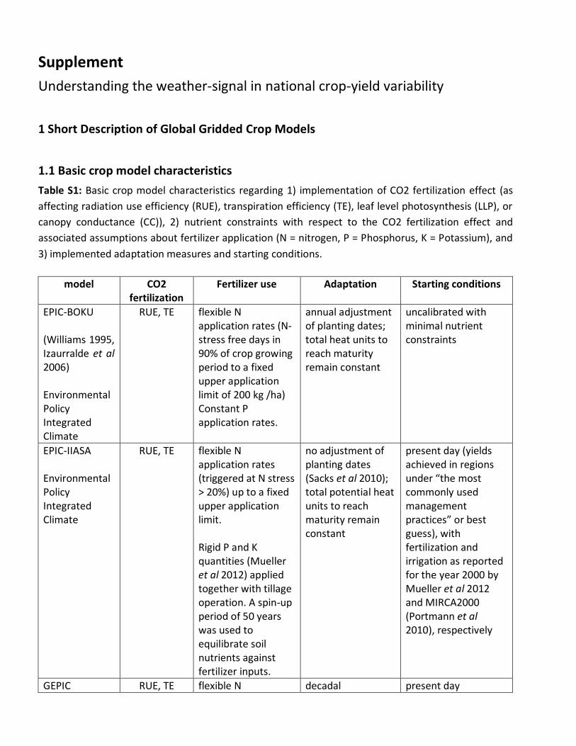
Table S1: Basic crop model characteristics regarding 1) implementation of CO2 fertilization effect (as
affecting radiation use efficiency (RUE), transpiration efficiency (TE), leaf level photosynthesis (LLP), or
canopy conductance (CC)), 2) nutrient constraints with respect to the CO2 fertilization effect and
associated assumptions about fertilizer application (N = nitrogen, P = Phosphorus, K = Potassium), and
3) implemented adaptation measures and starting conditions.
model CO2 fertilization
Fertilizer use Adaptation
Starting conditions
EPIC-BOKU (Williams 1995, Izaurralde et al 2006) Environmental Policy Integrated Climate
RUE, TE
flexible N application rates (N-stress free days in 90% of crop growing period to a fixed upper application limit of 200 kg /ha) Constant P application rates.
annual adjustment of planting dates; total heat units to reach maturity remain constant
uncalibrated with minimal nutrient constraints
EPIC-IIASA Environmental Policy Integrated Climate
RUE, TE flexible N application rates (triggered at N stress > 20%) up to a fixed upper application limit. Rigid P and K quantities (Mueller et al 2012) applied together with tillage operation. A spin-up period of 50 years was used to equilibrate soil nutrients against fertilizer inputs.
no adjustment of planting dates (Sacks et al 2010); total potential heat units to reach maturity remain constant
present day (yields achieved in regions under “the most commonly used management practices” or best guess), with fertilization and irrigation as reported for the year 2000 by Mueller et al 2012 and MIRCA2000 (Portmann et al 2010), respectively
GEPIC RUE, TE flexible N decadal present day

(Liu et al 2009, Williams et al 1989) GIS-based Environmental Policy Integrated Climate (EPIC) model
application based on N stress >10% (limitation of potential biomass increase due to N stress) up to an upper national application limit according to FertiStat, fixed present day P application rates following FAO FertiStat database (2010) (Anon n.d.)
adjustment of planting dates; total heat units to reach maturity remain constant decadal adjustment of winter and spring wheat sowing areas based on temperature
LPJ-GUESS LLP, CC no consideration of spatial and temporal changes in nutrient limitation
adjustment of planting dates cultivar adjustments are represented by variable heat units to reach maturity (Lindeskog et al 2013), adjustments are based on the average climate over the preceeding 10 years
uncalibrated
LPJmL (Bondeau et al 2007)
LLP, CC soil nutrient limiting factors are not accounted for
fixed sowing dates (Waha et al 2012b), total heat units to reach maturity remain constant
present day leaf Area Index (LAI), the Harvest Index (HI), and a scaling factor that scales leaf-level photosynthesis to stand level, are adjusted to reproduce observed yields on country levels
PEGASUS (Deryng et al 2011, 2014)
RUE, TE fixed N, P, K application rates (IFA national statistics)
adjustment of planting dates, variable heat units to reach maturity
present day

Predicting Ecosystem Goods And Services Using Scenarios
according to annual growing degree day accumulation
pDSSAT RUE, LLP, CC fixed N present day application rates
no adjustment of planting dates; total heat units to reach maturity remain constant
present day
pAPSIM RUE, TE, CC fixed N present day application rates (Müller and Lotze-Campen 2012)
no adjustment of planting dates; total heat units to reach maturity remain constant
present day
Table S2: List of daily weather variables used as input by the individual models.
EPIC-BOKU
EPIC-IIASA
GEPIC LPJ-GUESS
LPJmL pAPSIM pDSSAT Pegasus
Tmin X X X X X
Tmax X X X X X X
Tas X X X
Prec X X X X X X X X
wind speed X
shortwave radiation
X X X X X X X X
longwave radiation
X X X
relative humidity
X
1.2 Representation of soil water conditions
EPIC-IIASA:
The model contains routines to simulate soil water dynamics on a daily basis, including runoff, vertical
and horizontal subsurface storage routing and pipe flows, evaporation and transpiration as well as
interactions with water table. After a spin-up of 50 years, physical properties determining soil capacity
for water storage and water dynamics, such as field water capacity, wilting point, hydraulic
conductivity, bulk density and soil depth, were kept constant over time by resetting soil profile to its
initial conditions every year. Actual water content for a total of ten soil layers was calculated

dynamically and water content at the beginning of each year was carried over from the previous year.
This approach allows accounting for propagation of water deficit or excess across growing seasons
provided that soil water storage capacity does not change. Starting conditions of IIASA-EPIC were
calibrated to reproduce average observed yields within the reference period around year 2000
(Balkovič et al 2014, Xiong et al 2014, 2016). As a part of this calibration, the Hargreaves potential
evapotranspiration calculation routine was calibrated to reproduce appropriate water balance for a
given climate using the Princeton weather data (Sheffield et al 2006) while no interactions with ground
water table were considered.
The approach may lead to artificial yield variability when water dynamics are not represented
accurately. Resetting water content to a “default” initial value before growing season may lessen the
risk of artificial yield variability due to inappropriate hydrology. However, the timing of water reset
would be problematic. In addition, it would become impossible to trace cumulative effects stretching
across growing seasons.
EPIC-BOKU:
The representation of soil water conditions in EPIC-BOKU is basically identical to the representation in
EPIC-IIASA. In contrast to EPIC-IIASA the EPIC-BOKU model uses the Penman-Monteith equation to
compute potential evapotranspiration without considering interactions with ground water table.
GEPIC The representation of soil water conditions in GEPIC also largely follows the implementation in EPIC-
IIASA. In contrast to EPIC-IIASA, GEPIC only uses five soil horizons and has a fully dynamic soil profile
across each simulation decade as simulations are run for each decade with 30 years spin-up as
described in section 1.3 below.
LPJmL
The model uses a spinup of 200 years to initialized soil moisture and soil temperatures. Simulations are
conducted as transient simulations so that soil water is carried over to the next year. The description of
potential evapotranspiration is based on Priestley-Taylor (modified for transpiration). All crops are
simulated in parallel on different plots with no interaction during the growing periods. During fallow
periods, these plots are mixed, representing crop rotations of all crops simulated, averaging soil
moisture. The soil water conditions of the fallow-period plot on the day of sowing are used to initialize
the new soil conditions for crop-specific plots. Irrigated and rainfed fallow land are treated separately
so that no irrigation water in the soils can be transferred to rainfed land.
LPJ-GUESS
The model uses a spinup of 30 years to initialise soil moisture. As in LPJmL the description of potential
evapotranspiration is based on Priestley-Taylor. Simulations are conducted as transient simulations so
that soil water is carried over to the next year. All crops are simulated in parallel on different plots with

no interaction throughout the length of the simulation. There is no interaction between irrigated and
rainfed areas.
PEGASUS
In PEGASUS, the calculation of daily soil moisture follows a simple two‐layer bucket approach, driven
by the Priestley‐Taylor equation to estimate potential evapotranspiration. A more detailed description
of the surface energy and water budget calculation is given by Gerten et al 2004 and Ramankutty et al
2002. PEGASUS requires a 4-year spin-up to equilibrate soil water. As in the other models, simulations
are conducted as transient simulations so that soil water is carried over to the next year. All crops are
simulated in parallel on different plots with no interaction during the growing periods. Irrigated and
rainfed conditions are treated separately with no interaction between irrigated and rainfed cropland.
pAPSIM
The simulations initialized soil moisture every year, 3-5 months before planting, at 50% of the soil water
holding capacity. The simulations tracked runoff, drainage and soil water balance in up to 5 depth layers
(less for shallow soils) using soil and slope parameters based on data from the Harmonized World Soils
Database (HWSD). Evapotranspiration is calculated using the transpiration efficiency approach in which
biomass production is converted to water use based on the efficiency of transpiration for the given
crop and growth stage and the vapor pressure deficit.
pDSSAT
As in pAPSIM the simulations initialized soil moisture every year, 3-5 months before planting, at 50% of
the soil water holding capacity. The simulations tracked runoff, drainage and soil water balance in up to
4 depth layers (less for shallow soils) using soil and slope parameters based on data from the
Harmonized World Soils Database (HWSD). Potential evapotranspiration is calculated using the
Penman-Monteith equation.
1.3 Implementation of soil nutrient depletion in GEPIC
The GEPIC model accounts for soil nutrient depletion in low-input regions in order to achieve a robust
representation of present-day crop yields (Folberth et al 2012). To this end, the model is run for each
decade separately with a spin-up period of 30 years (see Figure S1). This may induce artificial yield
spikes at the beginning of each decade when soil nutrients are still highest.
Daily biomass increase is estimated in a two-step approach: 1) GEPIC estimates potential biomass
increase based on light interception and conversion of CO2 to biomass; 2) a limiting factor (maximum
of N or P deficit, temperature stress, water stress or aeration stress) is applied in order to derive the
actual biomass increase. Crop yields in nutrient deficient regions are therefore governed by nutrient

supply rather than climate. The fact that GEPIC selects only the most limiting crop stress on each day
makes it rather insensitive to climate variability in nutrient-deficient regions.
Figure S1: Schematic representation of decadal GEPIC runs.
2 Derivation of Growing and Extreme Degree Days
There are alternative empirical approaches that allow for a better approximation of non-linear
temperature effects on yields by accumulating the time spent within certain temperature bins over all
grid points within a considered region and estimating bin-specific temperature effects on overall yields
(e.g. Lobell et al., 2013; Wolfram Schlenker & Roberts, 2009). Schlenker et al. applied the approach to
U.S. county-level yield statistics to derive a critical temperature threshold beyond which yields start to
drop. While the authors applied a panel regression across a large number of time series of yield
observations from all U.S. counties, we are interested in the quantification of the weather-induced
variances of yields for individual countries. Since there are only 31 observations per country, a fully
flexible specification of bin-specific yield effects is not possible. Therefore, we apply a very similar
approach to the Growing Degree Days (GDD) approach of Schlenker et al., 2009 (see their SI) and Lobell
et al., 2011. In this case, GDDs and Extreme Degree Days (EDDs) are calculated at each grid point based
on daily maximum and minimum temperatures within the growing season (see Figure S2) and averaged
over the area of each country by weighting according to the crop-specific harvested area (MIRCA2000,
Portmann, Siebert, & Döll, 2010). The statistical model is described by
Yobs = 0 + 1GDD + EDD + P +
where indicates the deviation from the long-term trend.

Figure S2. Illustration of the derivation of Growing Degree Days (GDDs) and Extreme Degree Days
(EDDs) for a diurnal variation of temperatures as derived from daily maxima and mimima assuming a
sinusoidal evolution. While EDDs are represented by the blue area, GDDs are described by the area
under the curve between the two thresholds Lhigh and Llow. Both indicators are added up over the
growing season applying crop specific temperature thresholds (wheat: Llow = 3°C, Lhigh = 34°C; maize:
Llow = 8°C, Lhigh = 30°C; rice: Llow = 8°C, Lhigh = 35°C; soy: Llow = 7°C, Lhigh = 35°C).
3 Sensitivity to temporal shifts in reported or simulated crop yields

Figure S3. Analogous to Figure 2 of the main text but allowing for temporal shifts of the simulated time
series by one year back and forth. Colored symbols: maximum variance of the reported year-to-year
variability that is explained by individual crop models when 1) using the “default” time series or 2)
shifting the simulated time series by 1 year back and forth. Shifts are only considered if they increase
the explained variance by more than 0.2. Red diamonds: Highest variance explained by simple climate
indicators allowing for analogous shifts in time by one year back and forth. Black diamonds: Variance of
reported yield fluctuations explained by the multi-model mean of simulated yields where the mean is
calculated across the potentially shifted simulated time series. Shift were only applied if they increased
the crop model specific explained variance by more than 0.2. Countries are ordered according to the
highest variance explained by individual crop models. Grey polygons show the range from zero to the
highest explained variance provided by the process-based crop models for each country.
4 Explained variance based on different combinations of the climate indicators
Figure S4: Fraction of the variance of the reported crop yields that is explained by the considered
statistical models. The panels are analogous to Fig. 2 in the main text. The line thickness is according
the significance of the regression (lower p-value yields thicker lines).

5 Relationship between explained variances and the extent of the harvested land and standard deviation of the observed yields
Figure S5 Explained variances as provided by individual GGCMs (analogous to Figure 2 of the main text)
for all countries that are included in our study as main producers. Countries are ordered according to
the extent of crop-specific harvested area reported in MIRCA2000 (Portmann et al 2010).

Figure S6 Explained variances as provided by individual GGCMs (analogous to Figure 2 of the main text)
for all countries that are included in our study as main producers. Countries are ordered according to
the standard deviation of the de-trended time series of reported yields (FAO).
6 The role of the spatial resolution of climate input data
The correlation of the simulated yield time series based on 1) the high resolution climate input for the
European countries and 2) the aggregated low resolution version of this input (see section 2.5 of the
main text) is generally higher than 0.90, with the exception of maize in Spain (see Table S3 below).
There are no European countries belonging to the considered group of main producers of rice and soy.
The results support the assumption that the data at a higher resolution data than the 0.5° used in our
study is not essential. These results concur with a similar study for the US (Glotter et al 2014).

Table S3: Correlation of time series of crop yields simulated by LPJmL and forced by the high-resolution
climate input data and a lower-resolution version of the same climate data based on 1) bilinear
interpolation to the 0.5 degree grid, and 2) a conservative remapping of the data to the 0.5° grid,
where the values for each target cell represent the weighted sum (by contributing area) of all
contributing source cells.
Country
correlation conservative remapping
correlation bilinear remapping
wheat
Denmark 0.98 0.99
France 0.99 0.99
Germany 0.98 0.99
Hungary 0.99 0.99
Italy 0.98 0.98
Poland 1.00 1.00
Romania 0.98 0.99
Spain 0.99 0.99
Turkey 0.97 0.96
UK 0.96 0.92
maize
France 0.99 1.00
Germany 0.97 0.96
Spain 0.87 0.84
Hungary 0.99 0.99
Italy 0.94 0.94
Romania 0.97 0.98

7 Remaining correlations and standard deviations assuming full irrigation
Figure S7: Reproduction of recorded annual yield variations assuming present-day irrigation fractions
(MIRCA2000) and full irrigation. Black curves: De-trended recorded time series of national yields. Red
curves: De-trended simulated yield variations Ysim for the crop model that provide the highest
country-specific correlation with the FAO time series (identical to red lines in Figure 1 of the main text).
Irrigation fractions based on MIRCA2000. Blue curves: As for red curves but assuming full irrigation.
Results are shown for the three countries with the highest individual correlations. For each country
simulated and reported time series were scaled by the maximum of the absolute values of the three
time series. r2 refers to the correlation between reported and simulated time series under full
irrigation.

Figure S8: Analogous to Fig. 3 of the main text, but showing the standard deviations of the crop model
simulations assuming full irrigation.

8 Sensitivity to long-term changes in irrigation fractions The FAO statistics provides time series of “fraction of the cultivated area equipped for irrigation”. Data
are on a national level but not crop specific. For the sensitivity experiment, we assumed that the
extension of the fraction of the irrigated land is equal, but changing annually for all four crops
considered, i.e. the country averages of the simulated rain-fed and irrigated yields were weighted
according to identical annual “fraction of the cultivated area equipped for irrigation”.
Figure S9: Fraction of the variance of the reported yields that is explained by the crop model
simulations accounting for increasing irrigation fractions.
9 Sensitivity to longterm management Changes
The LPJmL model runs used for the sensitivity study are based on a slightly different model version than
the one used within the AgMIP/ISIMIP collaboration and shown in the main part of the paper.
Therefore, the correlations for the default run without any management adjustment (light green dots in
Fig. S5) are slightly different from the associated correlations shown in Fig. 2.

Figure S11: Comparison of explained variances for LPJmL “default” simulations and a model run
accounting for long-term management changes (see Methods). Light green dots: Explained variance for
the “default” setting. Dark green stars: Explained variance for the model runs accounting for
management changes. The order of the countries and the grey area is identical to Fig. 2 of the main
text. The dark green stars for maize in France and Germany, and rice in Egypt are not shown because
the correlation is negative. For four of the countries shown in Fig. S10, the management adjustment
leads to increases in explained variances. However, this unsystematic increase may be due to an
artificial adjustment to longer-term weather fluctuations (see Fig. S11 below).

Figure S12: Comparison of the de-trended yield variations from the LPJmL “default” run and a
sensitivity run where management was adjusted to reproduce the decadal averages of the reported
yields (see Methods section of the main text). Black lines: De-trended recorded time series of national
yields. Light green lines: De-trended simulated yield variations Ysim for the “default” model run.
Dashed dark green lines: Ysim for the model run accounting for long-term management changes.
Results are shown for the four countries with the highest individual deviations between both settings
shown in Figure S4. All time series were normalized by the individual maximum of the absolute values
of the country-specific FAO time series and the simulated time series. Explained variance for all other
simulations are included in Fig S10.

10 Sensitivity to Changes in Land Use Patterns
Figure S13: Comparison between explained variances of the standard run assuming fixed land-use and
irrigation patterns from MIRCA2000 and crop yields from LPJmL (green bars identical to Fig. 2), and a
sensitivity evaluation where the land-use patterns vary according to the historical changes in
agricultural area (red circles).
11 Sensitivity to a flexibile of sowing dates
In the standard LPJmL simulations considered in the main text, sowing dates are fixed. For comparison
we also calculated the explained variances based on alternative simulations where crop-specific,
weather-dependent adjustments of sowing dates were allowed. The start of the growing period is
assumed to be dependent either on the onset of the wet season or on the exceedance of a crop-
specific temperature threshold (Waha et al 2012a). The timing of sowing is dependent on precipitation
and temperature seasonality. In regions with precipitation seasonality, sowing starts at the onset of the
main wet season. Sowing dates of irrigated crops in LPJmL do not depend on precipitation seasonality.
In regions with temperature seasonality, sowing starts when daily average temperatures exceed a crop-
specific threshold.

Figure S14. Comparison between the explained variances of the standard run assuming fixed sowing
dates (light green circles identical to the bars in Fig. 2) and a sensitivity evaluation where the sowing
dates are allowed to vary according to the grid-point-specific evolution of temperatures and
precipitation (dark green stars).
Recommended