1
Review on Vortex-Induced Vibration for Wave Propagation Class
By Zhibiao Rao
What’s Vortex-Induced Vibration?
In fluid dynamics, vortex-induced vibrations (VIV) are motions induced on bodies interacting
with an external fluid flow.
The highly specialized subject of VIV is part of a number of disciplines, incorporating fluid
mechanics, structural mechanics, vibrations, computational fluid dynamics, acoustics, wavelet
transforms, complex demodulation analysis, statistics, and smart materials. They occur in many
engineering situations, such as bridges, stacks, transmission lines, aircraft control surfaces,
offshore structures, thermo wells, engines, heat exchangers, marine cables, towed cables, drilling
and production risers in petroleum production, mooring cables, moored structures, tethered
structures, buoyancy and spar hulls, pipelines, cable-laying, members of jacketed structures, and
other hydrodynamic and hydro acoustic applications (Sarpkaya, 2004).
How and Why does VIV Occur?
When a flow passes through a circular cylinder in the direction perpendicular to its axis, the VIV
will be seen. That’s because real fluids always present some viscosity, the flow around the
cylinder will be slowed down while in contact with its surface, forming the so called boundary
layer. At some points, however, this boundary layer can separate from the body because of its
excessive curvature. Vortices are then formed changing the pressure distribution along the
surface. These shedding vortices are called Von Karman Vortex Street. When the vortices are not
formed symmetrically around the body, different lift forces develop on each side of the body,
thus leading to motion transverse to the flow. This motion changes the nature of the vortex
formation in such a way as to lead to limited motion amplitude.
How to Model VIV of a Rigid Cylinder?
The force induced by vortex is periodic. Thus an equation of motion is introduced to represent
VIV of a cylinder oscillating in the transverse Y direction (normal to the flow) as follows:
� ������ + � ��
�� + � = � (1)
Where m is the structural mass, c the damping, k the constant spring stiffness, and F the fluid
force in the transverse direction.
2
The principal assumption is that the cross-flow excitation is a steady state periodic force, which
may be decomposed into a Fourier series. By the principle of superposition the response to each
Fourier component may be computed individually. The hydrodynamic force shown on the right
hand side of Equation (1) is in this case assumed to be the principal Fourier component of the
cross-flow excitation. A good approximation to the force is given by
�� � = �� ����������� + �� (2)
The steady state particular solution to this equation is given by
� � = ������ � (3)
Where � is 2�� and f the body oscillation frequency.
Plug Equations (2) and (3) into the Equation (1), we can get two equations, in which the time
dependent terms have cancelled out. Equation (4) establishes the equilibrium relationship
between the component of the fluid excitation in phase with stiffness and inertial forces in the
system.
�� − ����� = �� ������� ���� (4)
Equation (5) expresses the dynamic equilibrium that exists between the fluid lift force/length in
phase with the cylinder velocity and ���, the force/length required to drive the dashpot.
��� = �� ������������ (5)
Both Equations (4) and (5) are valid at any steady state excitation frequency.
An Example for a Typical VIV of Rigid Cylinder
Feng (1968) conducted in air with a single-degree-of freedom flexible cylinder with a relatively
large mass ratio and relatively large Reynolds number from 1x10⁴
to 5x10⁴. Figure 1 is the
classical self-excited oscillation plot showing the lock-in nature of the cylinder oscillation in
3
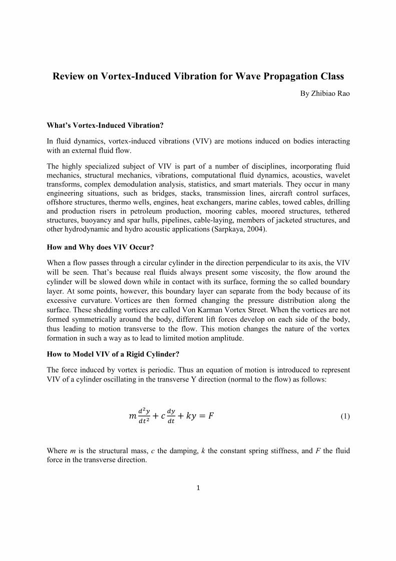
self-excited conditions. The two features of the plot show the reduced velocity (Vr=U/fairD)
plotted against both the amplitude-to-diameter ration (A/D) and the ratio of vortex-shedding
frequency to natural frequency (fex /f
air). The plot shows the sudden increase in oscillation
amplitude at Vr = 5. This lock-on continues to Vr=7.
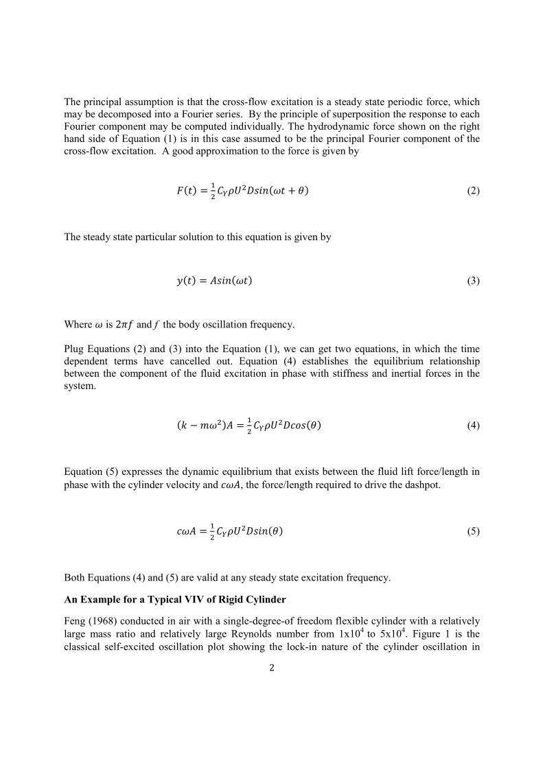
Figure 2 Lift coefficient is function of VIV amplitude (Vandiver, 2012)
The Figure 1 shows that VIV is not a small perturbation superimposed on a mean steady motion.
It is an inherently nonlinear, self-governed or self-regulated, multi-degree-of-freedom
phenomenon. It presents unsteady flow characteristics manifested by the existence of two
4
unsteady shear layers and large-scale structures. In other words, the VIV amplitude has a limited
value. However, from the Equation (2), lift coefficient seems be independent of amplitude. The
corresponding lift coefficient model should be adjusted to capture the nonlinear, self-governed or
self-regulated phenomenon. The real experimental data shows that the lift coefficient is the
function of VIV amplitude, shown in Fig.2.
What a Typical VIV Looks Like for Long Flexible Risers?
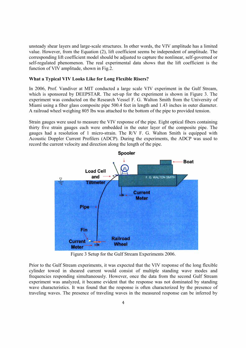
In 2006, Prof. Vandiver at MIT conducted a large scale VIV experiment in the Gulf Stream,
which is sponsored by DEEPSTAR. The set-up for the experiment is shown in Figure 3. The
experiment was conducted on the Research Vessel F. G. Walton Smith from the University of
Miami using a fiber glass composite pipe 500.4 feet in length and 1.43 inches in outer diameter.
A railroad wheel weighing 805 lbs was attached to the bottom of the pipe to provided tension.
Strain gauges were used to measure the VIV response of the pipe. Eight optical fibers containing
thirty five strain gauges each were embedded in the outer layer of the composite pipe. The
gauges had a resolution of 1 micro-strain. The R/V F. G. Walton Smith is equipped with
Acoustic Doppler Current Profilers (ADCP). During the experiments, the ADCP was used to
record the current velocity and direction along the length of the pipe.
Figure 3 Setup for the Gulf Stream Experiments 2006.
Prior to the Gulf Stream experiments, it was expected that the VIV response of the long flexible
cylinder towed in sheared current would consist of multiple standing wave modes and
frequencies responding simultaneously. However, once the data from the second Gulf Stream
experiment was analyzed, it became evident that the response was not dominated by standing
wave characteristics. It was found that the response is often characterized by the presence of
traveling waves. The presence of traveling waves in the measured response can be inferred by
5
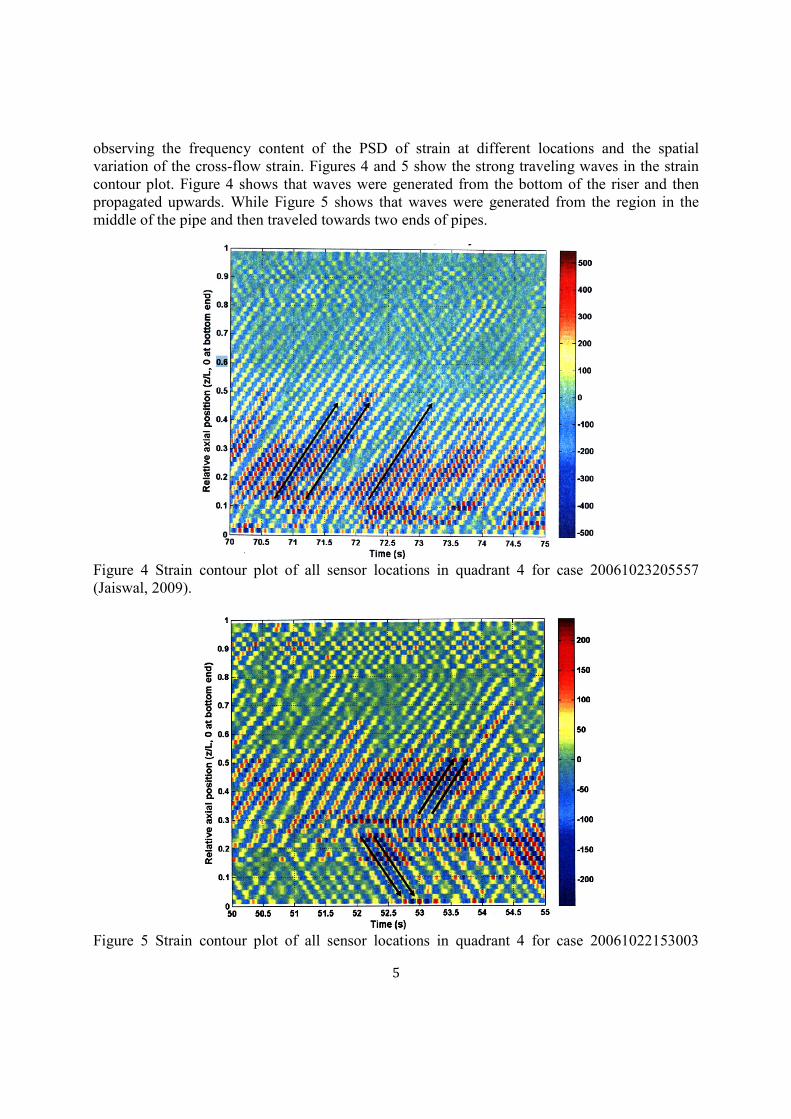
observing the frequency content of the PSD of strain at different locations and the spatial
variation of the cross-flow strain. Figures 4 and 5 show the strong traveling waves in the strain
contour plot. Figure 4 shows that waves were generated from the bottom of the riser and then
propagated upwards. While Figure 5 shows that waves were generated from the region in the
middle of the pipe and then traveled towards two ends of pipes.
Figure 4 Strain contour plot of all sensor locations in quadrant 4 for case 20061023205557
(Jaiswal, 2009).
Figure 5 Strain contour plot of all sensor locations in quadrant 4 for case 20061022153003
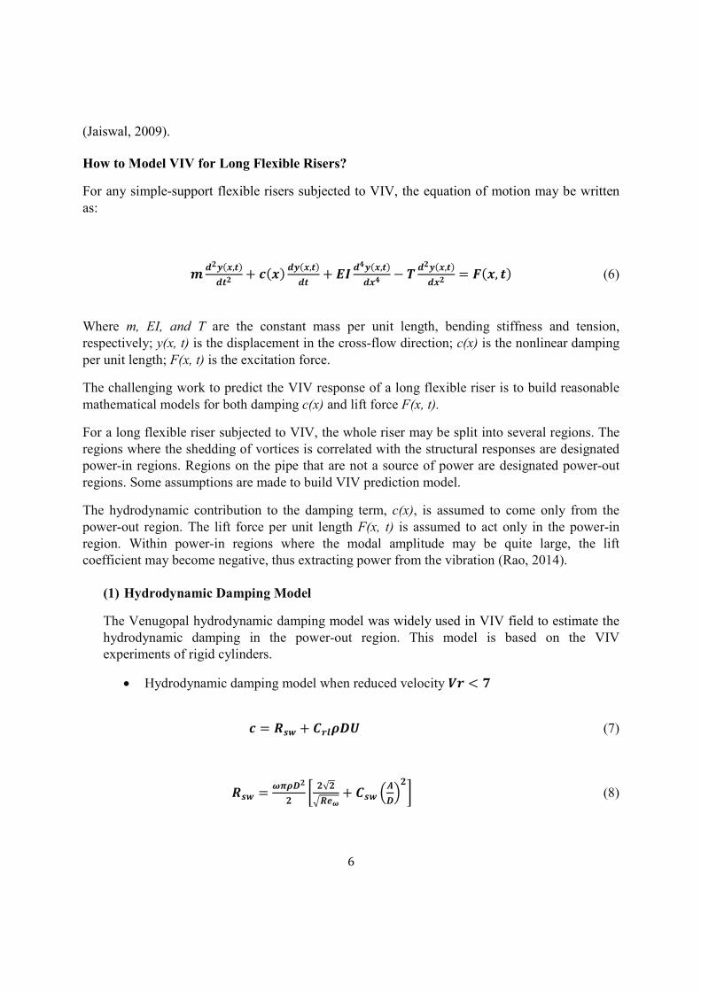
6
(Jaiswal, 2009).
How to Model VIV for Long Flexible Risers?
For any simple-support flexible risers subjected to VIV, the equation of motion may be written
as:
! "#$�%,'�"'# + (�%� "$�%,'�
"' + )* "+$�%,'�"%+ − , "#$�%,'�
"%# = -�%, '� (6)
Where m, EI, and T are the constant mass per unit length, bending stiffness and tension,
respectively; y(x, t) is the displacement in the cross-flow direction; c(x) is the nonlinear damping
per unit length; F(x, t) is the excitation force.
The challenging work to predict the VIV response of a long flexible riser is to build reasonable
mathematical models for both damping c(x) and lift force F(x, t).
For a long flexible riser subjected to VIV, the whole riser may be split into several regions. The
regions where the shedding of vortices is correlated with the structural responses are designated
power-in regions. Regions on the pipe that are not a source of power are designated power-out
regions. Some assumptions are made to build VIV prediction model.
The hydrodynamic contribution to the damping term, c(x), is assumed to come only from the
power-out region. The lift force per unit length F(x, t) is assumed to act only in the power-in
region. Within power-in regions where the modal amplitude may be quite large, the lift
coefficient may become negative, thus extracting power from the vibration (Rao, 2014).
(1) Hydrodynamic Damping Model
The Venugopal hydrodynamic damping model was widely used in VIV field to estimate the
hydrodynamic damping in the power-out region. This model is based on the VIV
experiments of rigid cylinders.
• Hydrodynamic damping model when reduced velocity ./ < 1
( = 234 + 5/6789 (7)
234 = :;78## < #√#
>2?:+ 534 @A
8B#C (8)
7
• Hydrodynamic damping model when reduced velocity ./ > 7
( = 5/F79#/: (9)
Where HIJ is the still water contribution; �KL is an empirical coefficient taken to be
0.18; HNO = OP�Q , a vibration Reynolds number; �IJ and �KR are two other empirical
coefficients, which at present are taken to be 0.2.
(2) Lift Coefficient Model
The lift coefficient model used for a long flexible cylinder is based on the experimental data
from a rigid cylinder. A rigid cylinder is forced to move at a certain frequency and amplitude
and the lift coefficient is measured from these experiments. Lift coefficient curve changing
with non-dimensional frequency and non-dimensional amplitude is built. For example, at the
non-dimensional frequency 1, the lift coefficient is changing with non-dimensional
amplitude like the Figure 2.
How Good Are These Models?
The Equation (6) could be solved with mode superposition method. Firstly, it evaluates which
modes are likely to be excited by the relationship of vortex shedding frequency and its natural
frequencies. The mode weight of each mode could be estimated by the iteration on the damping
coefficient and lift coefficient until the negative power due to damping is balanced by the
positive power due to lift force.
It should be noted that all damping and lift force models are based on the experimental data from
rigid cylinders rather than directly from long flexible cylinders. And all these predictions are
based on the assumption that the power-in region is known beforehand.
Swithenbank and Vandiver (2007) pioneered methods for locating the power-in region of long
flexible cylinders, using data from two tests conducted in the Gulf Stream. Two methods, the
coherence mesh and the reduced velocity, were presented to locate the source of VIV. The
coherence mesh method is based on the assumption that the large amplitude travelling waves are
expected to be coherent over a long range. This method fails to locate the power-in region when
VIV response is dominated by standing waves. The reduced velocity method is based on the
assumption that reduced velocity range from 5 to 7 is associated with large VIV response and is
assumed to be a power-in region. However, the reduced velocity method fails when the pipe is
partially covered with suppression devices under uniform flow. This is because the suppression
devices are able to cause the region to be power-out, even when the reduced velocity is in the 5
to 7 range.
8
In fact, the power-in region could be identified based on power balance from experimental data.
The region associated with positive time average power is considered the power-in region. This
method is more robust than those proposed by Swithenbank & Vandiver in 2007. It doesn’t
require the dominance of traveling wave and works for the pipe partially covered with
suppression devices under uniform and sheared flows.
The Equation (6) could be rewritten as an integral form as follows:
SS' T )dz5. + T SW
SX dz5. = T YZ dz5. − T [Z dz5. (10)
Where, \ is the energy density (energy per unit length) and ] is the energy flux, which passes
through the ends of the control volume in the axial direction. This energy flux is also known as
the instantaneous vibration intensity; Z is the rate of work done by the fluid excitation force and
_Z is the rate of work done by structural and hydrodynamic sources of damping. Both Z and _Z have units of power per unit length.
The power-in region is defined as that region where the power generated by the excitation force
is greater than the power dissipated by damping. In other words, the right hand side of Equation
(10) should be greater than zero in the power-in region. The results of identified power-in region
from VIV experiments could be used to benchmark a traditional method used to estimate the
power-in region.
How To Eliminate VIV?
Offshore marine risers and pipelines, exposed to ocean currents, are susceptible to VIV. Fatigue
damage due to VIV continues to cause significant problems in the design of structures. These
vibrations lead to fatigue which can limit the functional life of the offshore structures.
The circular cylinder will always be the preferred shape and the fluctuating lift will always be
there. It may be best to design around VIV and then avoid the situations that will produce VIV.
9
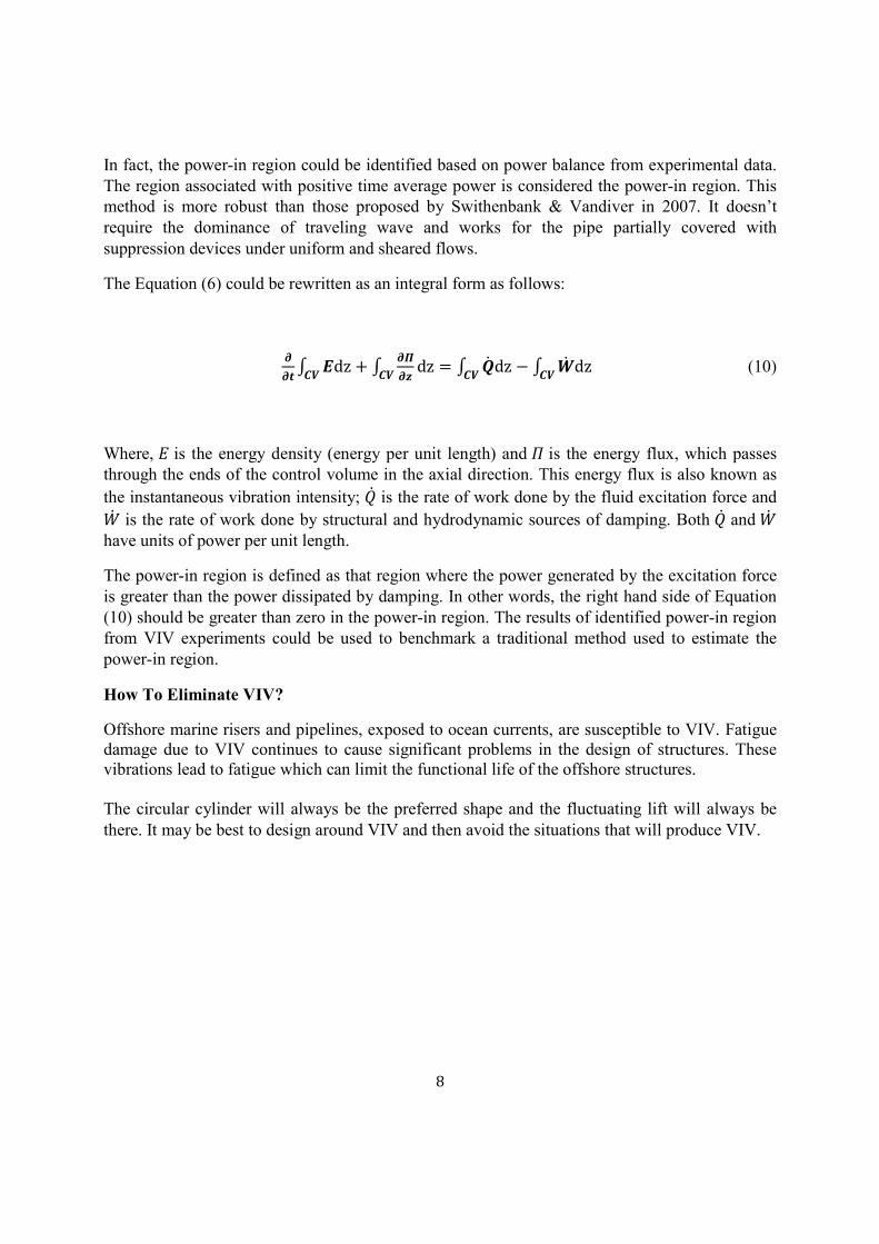
Figure 6 80mm diameter pipe covered with triple start helical strakes
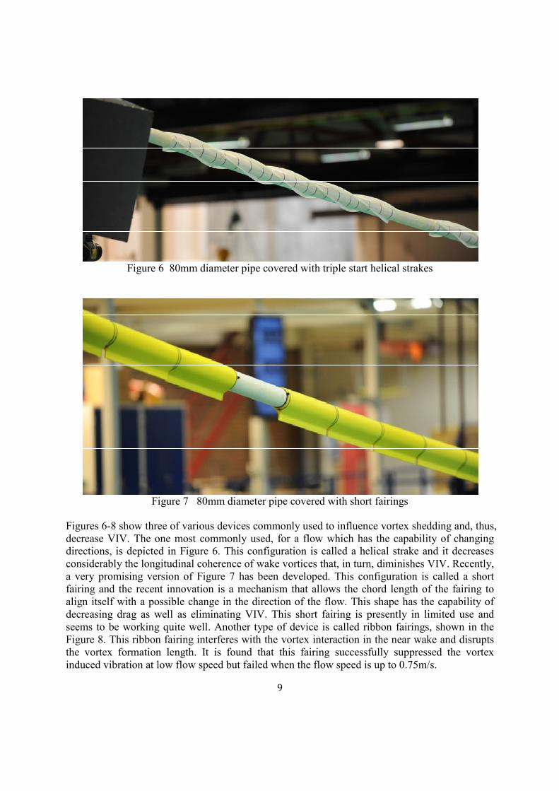
Figure 7 80mm diameter pipe covered with short fairings
Figures 6-8 show three of various devices commonly used to influence vortex shedding and, thus,
decrease VIV. The one most commonly used, for a flow which has the capability of changing
directions, is depicted in Figure 6. This configuration is called a helical strake and it decreases
considerably the longitudinal coherence of wake vortices that, in turn, diminishes VIV. Recently,
a very promising version of Figure 7 has been developed. This configuration is called a short
fairing and the recent innovation is a mechanism that allows the chord length of the fairing to
align itself with a possible change in the direction of the flow. This shape has the capability of
decreasing drag as well as eliminating VIV. This short fairing is presently in limited use and
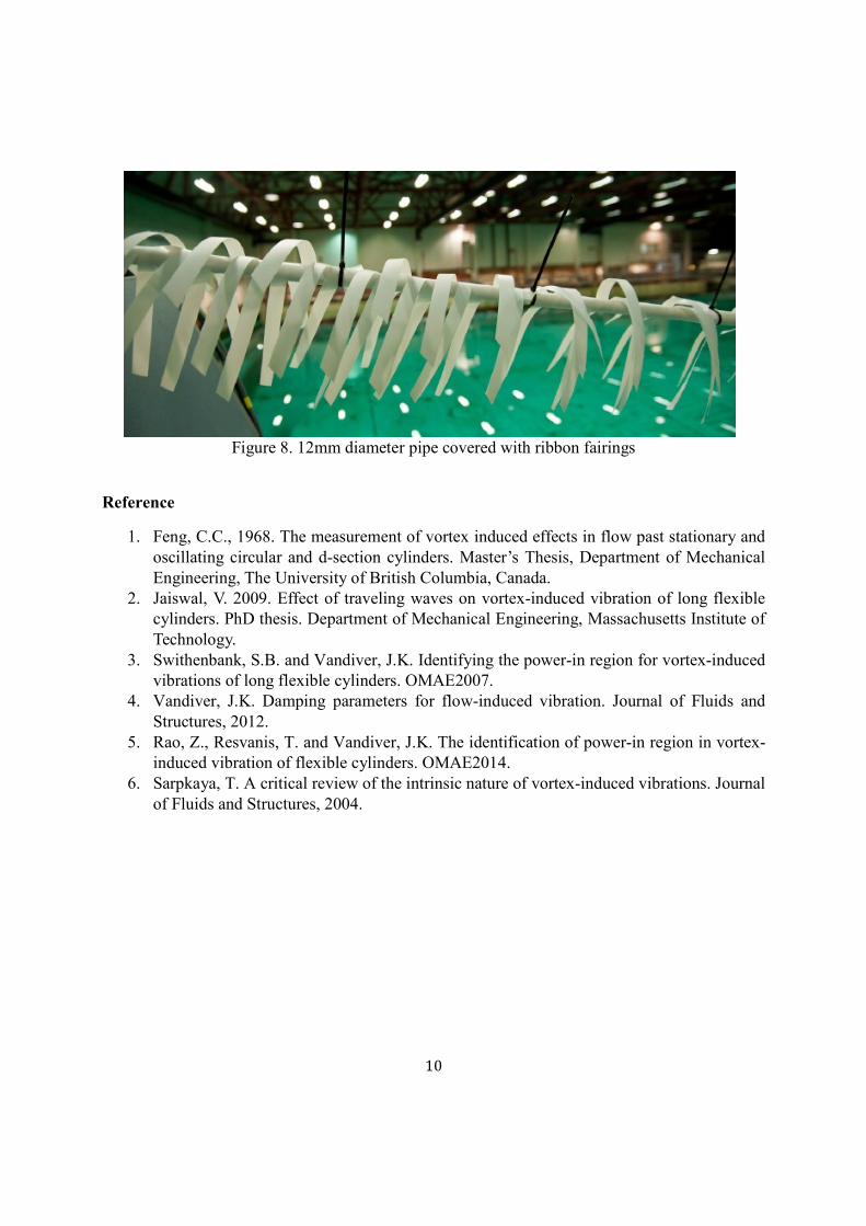
seems to be working quite well. Another type of device is called ribbon fairings, shown in the
Figure 8. This ribbon fairing interferes with the vortex interaction in the near wake and disrupts
the vortex formation length. It is found that this fairing successfully suppressed the vortex
induced vibration at low flow speed but failed when the flow speed is up to 0.75m/s.
10
Figure 8. 12mm diameter pipe covered with ribbon fairings
Reference
1. Feng, C.C., 1968. The measurement of vortex induced effects in flow past stationary and
oscillating circular and d-section cylinders. Master’s Thesis, Department of Mechanical
Engineering, The University of British Columbia, Canada.
2. Jaiswal, V. 2009. Effect of traveling waves on vortex-induced vibration of long flexible
cylinders. PhD thesis. Department of Mechanical Engineering, Massachusetts Institute of
Technology.
3. Swithenbank, S.B. and Vandiver, J.K. Identifying the power-in region for vortex-induced
vibrations of long flexible cylinders. OMAE2007.
4. Vandiver, J.K. Damping parameters for flow-induced vibration. Journal of Fluids and
Structures, 2012.
5. Rao, Z., Resvanis, T. and Vandiver, J.K. The identification of power-in region in vortex-
induced vibration of flexible cylinders. OMAE2014.
6. Sarpkaya, T. A critical review of the intrinsic nature of vortex-induced vibrations. Journal
of Fluids and Structures, 2004.
Recommended