Download pdf - Iterative continuous maximum-likelihood reconstruction method

Mathematical Methods in the Applied Sciences, Vol. 15, 275-286 (1992) MOS subject classification: 65 R 20

Iterative Continuous Maximum-likelihood Reconstruction Method

H. N. Multhei

Fachbereich Mathematik, Johannes Gutenberg-Unioersitat, Postfoch 39 80, Staudingerweg 9, W-6500 Mainz I , Germany

Communicated by W. Tornig

In this paper we continue our studying of the iterative maximum-likelihood reconstruction method. We consider only the continuous case and show some convergence properties of the algorithm. In the discrete case convergence has already been proved. An example demonstrating divergence of the iterative method shows how to handle the continuous case.

1. Introduction

The iterative maximum-likelihood reconstruction method (briefly called IM) was investigated in detail by Miilthei and Schorr [3,4]. The discrete iterative scheme as a method for image reconstruction in emission tomography was first systematically studied by Shepp and Vardi [S]. Global convergence for this case was shown later by Vardi et al. [6] who used a general result of Csiszir and Tusnidy [l]. A short and elementary proof of global convergence is given for the discrete IM in [4]. Kondor [2] applied the continuous IM to linear integral equations of the first kind with positive kernel and non-negative inhomogenity without answering the question of convergence. In this paper we only consider the continuous IM, which is defined in section 3. This

case is much more complicated than the discrete one. Convergence of the iterative scheme has been an open question, although many special properties of the continuous IM have been shown in [3, 41. The main difficulties arise from the fact that the domain of the log-likelihood functional A considered in section 2 is no longer compact.

In section 2, a maximization problem for A is investigated and a characterization of a solution is given. Using results from [4] we are able to prove new convergence properties of the IM in section 3. In section 4 we construct an example such that the maximization problem has no solution in the classical sense and the IM does not converge. On the other hand, the example suggests mapping the iterated functions of the IM into the closed range of the operator given by the kernel of A and studying the convergence in that set.

01 70-421 4/92/O40275- 12W6.00 0 1992 by B. G. Teubner Stuttgart-John Wiley 8c Sons, Ltd.

Received I S May 1991

276 H. N. Multhei

2. The maximization problem

In this section, we first repeat some definitions from [3]:

X:= { hEC[O, l]\{O}: h non-negative),

X + := { h E X : h positive),

X,:= { h e # : Jol h(x)dx = 1 , 1 In order to avoid unnecessary complications, we generally assume (as in [4]) that

the kernel k is a positive function in C [0, 13 normalized by

lo1 k ( x , y)dx = 1, YELO, 11.

Furthermore, we always assume that S E X l . This assumption is weaker than that given in [3,4]. There we additionally required positivity of g; therefore the results from this paper can only be applied if care is taken.

The concave functional A can be considered as the limiting case of the log- likelihood function of a sample from independent Poisson distributions [3]. In [3,4], the following maximization problem (MP) has been considered: maximize A(f) for fe X, . A solution of the MP is briefly called an M-function of A. The example in section 4 shows that such an M-function does not necessarily exist. This is not surprising, because XI is not compact in C[O, 13 with the sup-norm. There is another obvious possibility to take the set

JP := { f~ L , [0, 11 : 11 f ( 1 , = 1 and f non-negative almost everywhere),

containing X,, as the domain of A, but X : is not compact in L, [0, 11, either. Therefore, we proceed as follows.

Let d be the closure of the class

in CCO, 13. We first prove the following assertions.

Lemma 1. Let kmax:= ~ ~ k ~ ~ a , kmin:= min k ( x , y). Then x.yet0.11

Proox The assertions (a) and (b) are trivial for do. Therefore, they generally hold because the convergence in C[O, 11 is uniform. It is easy to see that the functions of do are equicontinuous. Furthermore, do is uniformly bounded because of (a). The ArzCla-Ascoli theorem then yields (c).

Iterative Maximum-likelihood Reconstruction Method 277

Remark. The closure of the set

in L, [0, 11 is identical with 58. This can be shown by using the facts that C[O, 11 is dense in L , [0, 13, especially &', in X i , and that the integral operator with kernel k is a continuous mapping from L,[O, 13 into C[O, 11, especially from &'; into H , . Therefore, it is sufficient to take X, in the definition of do.

Now it is appropriate to continue A to d. Let

g( x) In F( x) dx, F E d. A( F):= 1: Thus A ( F ) = A(f) holds for

F = lo1 k(. 3 Y )f(Y) dY, f E 2 1 *

A function F * E d maximizing A( F) for F E d is briefly called an M-function of A. Let

H := { h E 2, : h positive almost everywhere}.

Theorem 1.

(1) There exists an M-function of A. (2) For g E X an M-function of A is unique.

ProoJ A is a continuous functional and its domain at is compact owing to (c) of Lemma 1. Then it is well known that the first assertion holds. Furthermore, A is strictly concave because of g E X : and the strict concavity of the logarithm. This yields the uniqueness of an M-function of A. Remark. Iff * is an M-function of A, then

F* = lo1 u - 9 Y)f*(Y)dY

is an M-function of i, too. Note that the strict concavity of A is sufficient for the uniqueness of an M-function of A.

Now we are interested in characterizing an M-function of A. For that reason we need the following form of Jensen's inequality for integrals:

Furthermore, we introduce the directed Kullback-Leibler divergence of two densities h,,h,E&'l

[ 00, if the integral does not exist.

278 H. N. Miilthei

This non-negative functional induces some kind of directed distance measure on Sl and vanishes only for h , = h 2 . Furthermore, define

T(f)(y) := lo1 g‘xK:’ dx, y e [0, 13,

F(x) := J k(x, z)f(z)dz, XE[O, 1 3 , f ~ S ,

F := { h e S l : T ( h ) ( y ) < 1, YE[O, 13, where equality holds 0

for y with h(y) > O}.

Theorem 2. Thefunction f * is an M-function of A iJ; and only iJ f * E 5. I n general, the inequality

Nf) < Jol g(x) lng(x)dx

holds for fe Sl.

Remark. See [3], Theorem 1 and the Corollary on p. 145, and note that g E Sl has to be positive.

Proof: The inequality given above follows immediately from

1: g(x)lng(x)dx - A(f) = d(g,F) 2 0, f€Sl.

The proof of Theorem 1 in [3], showing that everyf* E 5 is an M-function of A, can be copied word for word by using Jensen’s inequality in the slightly more general version given here.

Let f * be an M-function of A and f := f* + E(P, where we require

Furthermore, let

Using Jensen’s inequality we have


For sufficiently small E this inequality yields the necessary condition

1; T(f*)(Y)cp(Y)dY G 0

by changing the order of integration. We consider the following two cases.

(1) Let U c [0, 11 be a neighbourhood of xo such that f*(x) > 0 for all x E U(xo). f, then belongs to S1 for all kcp with (2.1), supp cp c U and 0 < E < go = E ~ ( ( P )

if c0 is sufficiently small. Therefore, equality holds in (2.2) for such a function cp. Applying the well known lemma of du Bois-Reymond to (2.2) for this class of functions cp we obtain T ( f * ) ( y ) = c = const., Y E U . Let V c [0,1] be another neighbourhood with V n U = 125, f*(x) > 0, X E V, T(f*)(y) = c1 = const., Y E V. Trivially, there exists a permissible cp of the class (2.1) with supp cp c U u V, equality in (2.2), and

n n

Using (2.2) we have f1

This induces c , = c. Furthermore, the relation ri

yields T( f*NY) = 1, YELO, Il:f(y) > 0. (2.3)

(2) If xo is an isolated zero off* then T(f*)(x,) = 1 follows from continuity. Let f * ( x ) = 0 for all x in an interval W c [0, 13. Furthermore, let cp be an arbitrary function satisfying (2.1) with suppcp c U u W and

where U is just as above. Note that

cp(X)>O, X E w. Using (2.2) and (2.3) we obtain

r

Jw Varying cp in the permissible class induces

T(f*)(Y) G 1, Y E co, 11 : f (y) = 0. This completes the proof. Remark. T(f*)(xo) = 1 holds for an isolated zero xo off*.

280 H. N. Miilthei

3. The iterative method

As in [3,4] the continuous IM is defined by

L+1 = C(f.)9 f o e s , nENo3

W ) ( Y ) : = f ( y ) T ( f ) ( y ) , Y E LO, 111

where the operator G is given by

and maps X into Xl . Note that f* = G(f*) forf* E Y In the following, we first consider the defect

dn :=f. - G(f.)

=f. -L+1 =f.(l - T(f . )L n E N o .

Theorem 3. Let fo E JV + . Then

II dn I/ 1 0,

that is the IM is consistent with the fixed-point equation f = C(f) considered in L , LO, 11.

Proof: Using the Cauchy-Schwarz inequality and Theorem 7 [3], we have

IIdnII, = f . (y) l l - T(f.)(y)ldy lo1

In [3] (Theorem 7), it is shown that A(L), nEN, increases monotonically and converges to some real number A * = A * ( f o ) , f o ~ X + + , as n -+ co. Let

A~ := SUP A(S) = max & F ) . f E X , F € d

Trivially, we have A* G As. It is an open question whether equality holds. Let

Fn(x) := j: k ( x , y ) ~ ( y ) d y , n E ~ 0 ,

then we can prove the following theorem.

Theorem 4. Let Y # 0 . Then for arbitrary J, E 3' + :

(1) A(f.), n E N, increases monotonically and converges t o As = A( f *), f* E Y. (2) For gE X : F,, n E No, converges uniformly t o the unique M-function F* of as

n -, 00, where

Iterative Maximum-likelihood Reconstruction Method 28 1

Remark. Because of (3. l), f:,ft E F imply

IO1 k ( . , Y ) C f : ( Y ) -f:(Y)IdY = 0

for g E X ' : .

Pro05 According to Theorem 4 [4], we have forf= G ( f ) e X 1 andf,EX'+

d ( f , f , + 1) G Wf,) - "f) - A(L)I, n E N, (3.2) because the proof of (3.2) remains valid for g E X , . Trivially, f * ~ F induces f* = G(f*) and A(f*) = A, becausef* is an M-function of A. Therefore, (3.2) yields

0 < d( f* , f ,+ i ) < d(f*,f,), ~ E N .

Hence d(f*,f.), nE N, decreases monotonically and converges to a non-negative real number as n + OD. On the other hand,f* €9 and (3.2) induces

0 G Nf*) - Nf.1 G 4f*, i) - 4/*, f,+ 1 ) .

This proves the first assertion. The related sequence { F,},"=, belongs to do and therefore provides a compact set

in d c C[O, 11. Thus it follows that there exists a uniformily convergent subsequence. Let { F,,};,, be such a subsequence with the limiting point

F := lim F,, ~ d . i - m

The uniforrm convergence of this subsequence 'induces

ACf,,) - W). I - m

From Theorem 1 we conclude that there exists a unique M-function F* of such that (3.1) holds. The first assertion of Theorem 4 then yields i( F) = As = A( F*) . There- fore, the M-functions F and F* must be identical, that is the sequence {F,}:=o has, with respect to the sup-norm, the only limiting point F*. This completes the proof.

Corollary 1. Let f * E zl be a solution of the integral equation

JO1t(X,Y)f*(Y)dY = g ( x ) , XECO, 11, gcJfJ1 n X + .

Then F,, n E No, converges un$ormly to g for everyf,E&'+ as n -, co and

As = 1; g ( x ) In g ( x ) d x .

Proof. Trivially,f* belongs to F. Theorem 4 then yields the proof.

(3.3)

Remark. The Corollary is a useful result for the IM applied to this special, but important, class of integral equations (3.3). Indeed (3.3) has been the starting point of the investigations in [l, 31.

The question of convergence still remains open for the case where an M-functionf*

282 H. N. Miilthei

of A, that is a function f* E F, does not exist. We prove the following result.

Theorem 5. Let fo E X + and

L(x) 2 E > 0, XE[O, 13, nEN.

Then

(1) A(f.) - A, monotonically increasing,

(2) Fn - F * unijbrrnly for g E X : , n - m

n - m

where F * is the only M-function of A. Pro05 It is known that A(J) converges to some real number A * = A*(&). Assuming A * < As we can conclude by continuity arguments that there exists a functionfEXl satisfying A * < A(f). This induces the existence of a positive constant co such that

by using Jensen's inequality and changing the order of integration. From (3.4) it follows that

1 + c < ~olf(y)T(f.)(y)dy, nEN, c := exp(co) - 1 > 0, (3.5)

and, in particular, we can conclude

II W J l t m 3 1 + c, nEN. (3.6) On the other hand, we have

where

see Theorem 3. This leads to a contradiction to (3.5). Therefore, we have A * = As. The second assertion of Theorem 5 can be shown in an analogous way to the proof of Theorem 4.

The inequality (3.6) gives reason for the following conjecture.

Conjecture. Theorem 5 can be proved without the positivity assumption on fn, nE N.


4. An example

In complete analogy to the example in the discrete case [4], we consider the following somewhat extreme example with additional special properties of g and k:

g E S l : g(x) = 0, X E [ ~ , 1],0 < 6 < 1, 6 fixed,

k:k(x,y) = K(y),XE[O,6], I C E # + .

Thus the normalization condition for k yields

0 < B K ( Y ) = 1- k(x,y)dx < 1. (4.1) jd l

It is not a problem to construct such a kernel k E C[O, 1 J2. It is easy to see that the integral equation (3.3) has no solution in XI. The functional A has the special form

Hence, it is easy to see that exp(A,) = K, := 11 K 11 ,. If there exists a non-trivial interval J , where

K(Y) = K , , Y E J,

we can ensure the existence of functions ~ * E F with suppf* c J such that A(f*) = A,, especially, we have for such a functionf*

T(f*)(Y) = K ( Y ) / K , , YELO, 11. On the other hand, we have A(f) < A,, feX1, for a function K being almost everywhere different from K , such that there is no function f * E F. If ~ ( j ) = K,, trivially, k ( . , j ) E d is an M-function of A that is not unique in general because of the assumption about g.

The iterated functionsf, are given by

where

J,:= fo(z)K(z)"dz, & E X + , EN.

Note that f, is determined by K and fo. Furthermore, sd

Jn+l/Jn, XECO, 61,

Therefore,

A(f , ) = A ( F , ) = lnJ,+,/J,, EN.

What can be said about the convergence off. and F , as n + co? Theorems 4 and 5 must not be applied to this example because the assumption g E # is violated. Let us

284 H. N. Multhei

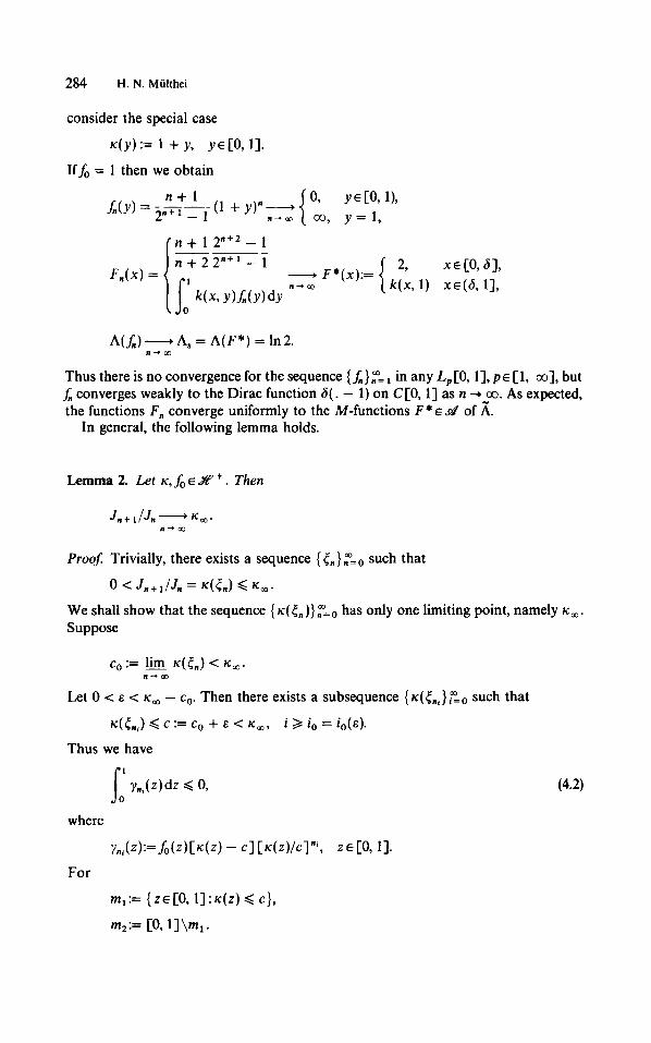
consider the special case

t i ( y ) := 1 + y, YE [O, I]. If& = 1 then we obtain

f n + 1 2n+2 - 1

A(f.)-As = A ( F * ) = In2. n - m

Thus there is no convergence for the sequence { L}:= in any LJO, 13, P E [l, 001, but f. converges weakly to the Dirac function 6(. - 1) on C[O, 13 as n -, co. As expected, the functions F, converge uniformly to the M-functions F* ~d of A.

In general, the following lemma holds.

Lemma 2. Let K, fo E &' + . Then

Proof: Trivially, there exists a sequence { t,,}:==, such that

0 < J n + I / J n = K ( t n ) G K,.

We shall show that the sequence { ~(t,,)}:=~ has only one limiting point, namely K,. Suppose

CO := !hJ K ( t , ) < K m . n - r m

Let 0 < E < t i , - co. Then there exists a subsequence { ~(<,,~},?i~ such that

~ ( t , , ) < c := co + E < K ~ , i 2 io = i O ( E ) .

Thus we have r i


we obtain

This is a contradiction to (4.2) and proves Lemma 2.

Corollary 2. Let K,& E X? +. Then -

A(L) = h ( F n ) = lnJ,+,/J, -lnK, = A,. n-. m

5. An extension

The investigations of MP and IM show that the strict concavity of the logarithm is an essential assumption. Therefore, the following generalization of A is possible, for example:

A(f):= lo1 g(x)L ( jol k(x, Y)f(Y)dY dx, f G J f 1 , ) where

L€C2(c, d):Ckrnin, krnaxI c (c, d ) ,

L’(z) > 0, (5.1)

L”(z) < 0, Z€(C, d). (5.2)

Thus L is strictly increasing and strictly concave; and (c,d) is allowed to be un- bounded. The addition theorem of the logarithm offered above the possibility of using Jensen’s inequality. In this case, the Taylor formula,

and

1

L(z) = L(zo) + (z - zo)L’(zo) + ( z - zo)2 [ tL”[z - t(z - zO)] dt, Jo

(5.3) can be helpful because the remainder is not positive. Using the ideas of the second part of the proof of Theorem 2 and considering (5.1), we easily obtain the following generalization of T:

286 H. N. Miilthei

Thereby, the Kuhn-Tucker set I and the iteration mapping G : Zl + are again well defined.

A lot of the given theory can be carried out for this generalized IM in the same way. For instance, Theorems 1 and 2 remain valid with the exception of the inequality in Theorem 2. As an application of (5.3) we show that every functionf*EF is an M-function of A:

Nf*) - Nf) = g(x)CL(F*(x)) - UF(x) ) ldx , f E J f 1 , sd = lo1 g(x)L’(F*(.x))[F*(x) - F(x)]dx + R, (5.4)

where

Because of (5.2) R is non-negative. Furthermore,f*EI and (5.1) yield for the first term in (5.4)

Thus f * is an M-function of A. On the other hand, we have for a solutionf* of the integral equation (3.3)

T(f*3(Y) = g(x)L‘(g(x))k(x, Y)dX g(z)2L’(g(Z))dz, sd / sd which does not generally induce f* E I. Trivially, L := log provides an exception. Therefore, the generalized IM is not appropriate for treating the important class of integral equations (3.3) numerically and we do not continue its investigation.

References

I . Cziszir, I. and Tusnidy, G. ‘Information geometry and alternating minimization procedures’, Statistics

2. Kondor, A., ‘Method of convergent weights-an iterative procedure of solving Fredholm’s integral

3. Miilthei, H. N. and Schorr, B., ‘On an iterative method for a class of integral equations of the first kind‘,

4. Miilthei, H. N. and Schorr, B., ‘On properties of the iterative maximum likelihood reconstruction

5. Shepp, L. A. and Vardi, Y., ‘Maximum likelihood reconstruction for emission tomography’, l E E E Trans.

and Decisions, Suppl. Issue, 1, 205-237 (1984).

equations e t h e first kind’, Nuclear Insrrwn. Methods, 216, 177-181 (1983).

Math. Meth. in the Appl. Sci., 9, 137-168 (1987).

method’, Math. Merh. in the Appl. Sci., 11, 331-342 (1989).

Medical Imaging, MI-1, 113-122 (1982). 6. Vardi, Y., Shepp, L. A. and Kaufman, L., ‘A statistical model for positron emission tomography’, J A S A ,

SO, 8-37 (1985).