Embed Size (px)
Citation preview
A Novel Methodology for Iterative Image Reconstruction in
SPECT Using Deterministic Particle Transport
Katherine Royston
Dissertation submitted to the Faculty of theVirginia Polytechnic Institute and State University
in partial fulfillment of the requirements for the degree of
Doctor of Philosophyin
Nuclear Engineering
Alireza Haghighat, ChairYue J. Wang
Mark R. PaulKenneth H. Wong
Celine HinCe Yi
March 23, 2015Arlington, Virginia
Keywords: deterministic transport, SPECT, image reconstruction
Copyright 2015, Katherine Royston
A Novel Methodology for Iterative Image Reconstruction in SPECT UsingDeterministic Particle Transport
Katherine Royston
ABSTRACT
Single photon emission computed tomography (SPECT) is used in a variety of med-ical procedures, including myocardial perfusion, bone metabolism, and thyroid func-tion studies. In SPECT, the emissions of a radionuclide within a patient are counted ata gamma camera to form a 2-dimensional projection of the 3-dimensional radionuclidedistribution within the patient. This unknown 3-dimensional source distribution can bereconstructed from many 2-dimensional projections obtained at different angles aroundthe patient. This reconstruction can be improved by properly modeling the physics in thepatient, i.e., particle absorption and scattering. Currently, such modeling is done usingstatistical Monte Carlo methods, but deterministic codes have the potential to offer fastcomputation speeds while fully modeling particle interactions within the patient. De-terministic codes are not susceptible to statistical uncertainty, but have been over-lookedfor applications to nuclear medicine, most likely due to their own limitations, includingdiscretization and large memory requirements.
A novel deterministic reconstruction methodology for SPECT (DRS) has been de-veloped to apply the advantages of deterministic algorithms to SPECT iterative imagereconstruction. Using a maximum likelihood expectation maximization (ML-EM) algo-rithm, a deterministic code can fully model particle transport in the patient in the forwardprojection step, without the need of a large system matrix. The TITAN deterministic trans-port code has a SPECT formulation that allows for fast simulation of SPECT projectionimages and has been benchmarked through comparison with results from the SIMINDand MCNP5 Monte Carlo codes in this dissertation. The TITAN SPECT formulation hasbeen improved through a modified collimator representation and full parallelization. TheDRS methodology has been implemented in the TITAN code to create TITAN with ImageReconstruction (TITAN-IR). The TITAN-IR code has been used to successfully reconstructthe source distribution from SPECT data for the Jaszczak and NCAT phantoms. Extensivestudies have been conducted to examine the sensitivity of TITAN-IR image quality to de-terministic parameter selection as well as collimator blur and noise in the projection databeing reconstructed. The TITAN-IR reconstruction has also been compared with other re-construction algorithms. This novel image reconstruction methodology has been shownto reconstruct images in short computation times, demonstrating its potential in a clinicalsetting with further development.

Dedication
To my parents and my husband
iii

Acknowledgements
I would like to express my gratitude to Dr. Alireza Haghighat, my advisor, for his patience
and guidance in this work. His advice enabled me to successfully overcome the many
obstacles I encountered. I thank my advisory committee for their time and feedback,
especially Dr. Ce Yi for taking the time to work with me and provide vital assistance in the
use of the TITAN code. I would like to thank my fellow graduate students, Will Walters
and Nate Roskoff, for providing advice and discussion of problems as they arose as well
as many a good laugh. My family deserves acknowledgement for their endless support
and encouragement of my academic studies. My parents have taught me to always do
my best and provided me with the skills to succeed. I would like to thank my husband
Sean for always being there and having in faith in me.
iv
Contents
1 Introduction 1
2 Literature Review 4
2.1 SPECT Background . . . . . . . . . . . . . . . . . . . . . . . . . . . . . . . . . 4
2.2 Image Reconstruction Background . . . . . . . . . . . . . . . . . . . . . . . . 5
2.3 SPECT Simulation and Reconstruction Codes . . . . . . . . . . . . . . . . . . 9
2.4 Iterative Reconstruction Research . . . . . . . . . . . . . . . . . . . . . . . . . 10
3 Theory 13
3.1 Solving the Linear Boltzmann Equation . . . . . . . . . . . . . . . . . . . . . 13
3.2 The TITAN Code . . . . . . . . . . . . . . . . . . . . . . . . . . . . . . . . . . 19
3.2.1 Hybrid Formulation . . . . . . . . . . . . . . . . . . . . . . . . . . . . 19
3.2.2 Parallel Implementation . . . . . . . . . . . . . . . . . . . . . . . . . . 20
3.2.3 SPECT Formulation . . . . . . . . . . . . . . . . . . . . . . . . . . . . 22
3.3 ML-EM Reconstruction . . . . . . . . . . . . . . . . . . . . . . . . . . . . . . . 25
3.4 Novel Deterministic Reconstruction Methodology . . . . . . . . . . . . . . . 27
4 Analysis of SPECT Algorithm in TITAN 29
4.1 Projection Comparison with SIMIND . . . . . . . . . . . . . . . . . . . . . . . 30
4.2 Projection Comparison with MCNP5 . . . . . . . . . . . . . . . . . . . . . . . 33
4.3 Projection Comparison with Experiment . . . . . . . . . . . . . . . . . . . . . 37
5 Enhancement of SPECT Algorithm in TITAN 40
v

Iterative Image Reconstruction in SPECT Using Deterministic Transport
5.1 Parallel Computation . . . . . . . . . . . . . . . . . . . . . . . . . . . . . . . . 40
5.1.1 Parallel Processing Metrics . . . . . . . . . . . . . . . . . . . . . . . . 40
5.1.2 Parallel Performance of SPECT Simulation . . . . . . . . . . . . . . . 42
5.1.3 Parallelized SPECT Projection Algorithm . . . . . . . . . . . . . . . . 44
5.2 Weighted Circular Ordinate Splitting . . . . . . . . . . . . . . . . . . . . . . . 47
6 Implementation of the Novel Image Reconstruction Methodology 53
6.1 DRS Methodology . . . . . . . . . . . . . . . . . . . . . . . . . . . . . . . . . 53
6.2 Analysis of DRS methodology . . . . . . . . . . . . . . . . . . . . . . . . . . . 56
6.2.1 Framework Implementation . . . . . . . . . . . . . . . . . . . . . . . 56
6.2.2 Phantom Studies . . . . . . . . . . . . . . . . . . . . . . . . . . . . . . 57
7 Development of TITAN-IR Algorithm 71
7.1 TITAN-IR Algorithm . . . . . . . . . . . . . . . . . . . . . . . . . . . . . . . . 71
7.2 TITAN-IR Implementation . . . . . . . . . . . . . . . . . . . . . . . . . . . . . 73
7.2.1 Parallel Implementation . . . . . . . . . . . . . . . . . . . . . . . . . . 74
7.2.2 OS-EM Implementation . . . . . . . . . . . . . . . . . . . . . . . . . . 75
7.3 Quality Metrics . . . . . . . . . . . . . . . . . . . . . . . . . . . . . . . . . . . 76
8 Analysis of TITAN-IR 79
8.1 Jaszczak Phantom with Cold Spheres . . . . . . . . . . . . . . . . . . . . . . . 79
8.1.1 Noiseless Projection Data with No Collimator Blur . . . . . . . . . . 82
8.1.2 Noisy Projection Data with No Collimator Blur . . . . . . . . . . . . 92
8.1.3 Noisy Collimated Projection Data . . . . . . . . . . . . . . . . . . . . 95
8.1.4 Comparison with Other Reconstruction Methods . . . . . . . . . . . 100
8.1.5 Computation Time . . . . . . . . . . . . . . . . . . . . . . . . . . . . . 109
8.2 NCAT Phantom . . . . . . . . . . . . . . . . . . . . . . . . . . . . . . . . . . . 112
8.2.1 Noiseless Projection Data with No Collimator Blur . . . . . . . . . . 115
8.2.2 Noisy Collimated Projection Data . . . . . . . . . . . . . . . . . . . . 118
8.2.3 Computation time . . . . . . . . . . . . . . . . . . . . . . . . . . . . . 122
vi
Table of Contents
9 Conclusions and Future Work 125
Bibliography 130
Appendix A Reconstruction Script 138
Appendix B TITAN-IR Input and Features 147
B.1 Reconstruction Input Block . . . . . . . . . . . . . . . . . . . . . . . . . . . . 147
B.2 Contrast . . . . . . . . . . . . . . . . . . . . . . . . . . . . . . . . . . . . . . . 149
B.3 Sparse System Matrix Format . . . . . . . . . . . . . . . . . . . . . . . . . . . 150
vii

List of Figures
3.1 Schematics of the directions in a quadrature set in one octant . . . . . . . . . 15
3.2 Source iteration in the TITAN code . . . . . . . . . . . . . . . . . . . . . . . . 21
3.3 Example schematic of a fictitious quadrature set with circular ordinatesplitting. . . . . . . . . . . . . . . . . . . . . . . . . . . . . . . . . . . . . . . . 23
3.4 Circular ordinate splitting (COS) with 2 circles and 6 directions per circle. . 24
4.1 Sagittal slice through TITAN geometry on NCAT phantom with regionsusing the SN and ray-tracing solvers indicated . . . . . . . . . . . . . . . . . 30
4.2 Projection images generated by the SIMIND code for (a) anterior, (b) leftlateral, (c) posterior, and (d) right lateral views . . . . . . . . . . . . . . . . . 31
4.3 Projection images generated by the TITAN code for (a) anterior, (b) leftlateral, (c) posterior, and (d) right lateral views . . . . . . . . . . . . . . . . . 31
4.4 (a) Vertical and (b) horizontal profiles through heart in anterior projectionsfrom TITAN and SIMIND. . . . . . . . . . . . . . . . . . . . . . . . . . . . . . 32
4.5 MCNP5 anterior projection images for collimator cases . . . . . . . . . . . . 34
4.6 TITAN anterior projection images for collimator cases . . . . . . . . . . . . . 34
4.7 Case 1 profiles through MCNP5 and TITAN projection images: (a) verticaland (b) horizontal . . . . . . . . . . . . . . . . . . . . . . . . . . . . . . . . . . 36
4.8 Case 2 profiles through MCNP5 and TITAN projection images: (a) verticaland (b) horizontal . . . . . . . . . . . . . . . . . . . . . . . . . . . . . . . . . . 36
4.9 Case 3 profiles through MCNP5 and TITAN projection images: (a) verticaland (b) horizontal . . . . . . . . . . . . . . . . . . . . . . . . . . . . . . . . . . 36
4.10 Dynamic cardiac phantom being imaged by a prototype bedside SPECTsystem. . . . . . . . . . . . . . . . . . . . . . . . . . . . . . . . . . . . . . . . . 38
viii
Table of Contents
4.11 Slice through contoured CT scan of the dynamic cardiac phantom . . . . . . 38
4.12 Anterior projection images of the dynamic cardiac phantom. . . . . . . . . . 38
4.13 Profiles through anterior projection images of the dynamic cardiac phantom 39
5.1 Parallel speedup for TITAN and MCNP5 as a function of number of pro-cessors . . . . . . . . . . . . . . . . . . . . . . . . . . . . . . . . . . . . . . . . 43
5.2 Projection of detector surface area to front of collimator along a split direc-tion; flux is weighted by the overlapping area . . . . . . . . . . . . . . . . . . 48
5.3 Example of splitting directions for two circles and a splitting order of 6 . . . 48
5.4 Phantom geometry for WCOS testing . . . . . . . . . . . . . . . . . . . . . . 49
5.5 TITAN and MCNP5 (1σ 0.8− 3.6%) flux distributions for LEGP collimator(1.65) . . . . . . . . . . . . . . . . . . . . . . . . . . . . . . . . . . . . . . . . . 50
5.6 TITAN and MCNP5 (1σ 0.4− 4.4%) flux distributions for LEHS collimator(4.29) . . . . . . . . . . . . . . . . . . . . . . . . . . . . . . . . . . . . . . . . . 50
6.1 DRS methodology workflow . . . . . . . . . . . . . . . . . . . . . . . . . . . 55
6.2 Reference source distribution with source strengths of 2 in white and 1 ingray . . . . . . . . . . . . . . . . . . . . . . . . . . . . . . . . . . . . . . . . . . 58
6.3 TITAN 3-dimensional model . . . . . . . . . . . . . . . . . . . . . . . . . . . 58
6.4 Reference sinogram for 120 projection angles produced by SIMIND . . . . . 59
6.5 Projection image comparison with SIMIND for different TITAN meshings . 61
6.6 Sinograms generated by TITAN (S20 DDZ) over 180 . . . . . . . . . . . . . . 64
6.7 Reconstructed source distributions from TITAN 180 sinograms (S20 DDZ) . 64
6.8 Sinograms generated by TITAN (S20 DTW) over 180 . . . . . . . . . . . . . 64
6.9 Reconstructed source distributions from TITAN 180 sinograms (S20 DTW) 64
6.10 Reconstructed source distributions from TITAN 360 sinograms (S20 DDZ) . 65
6.11 Reconstructed source distributions from TITAN 360 sinograms (S20 DTW) 65
6.12 Horizontal profile through reconstructed source distribution with DDZscheme . . . . . . . . . . . . . . . . . . . . . . . . . . . . . . . . . . . . . . . . 66
6.13 Horizontal profile through reconstructed source distribution with DTWscheme . . . . . . . . . . . . . . . . . . . . . . . . . . . . . . . . . . . . . . . . 66
6.14 Reconstructed source distributions using the system matrix only . . . . . . . 67
ix

Table of Contents
6.15 Horizontal profile through reconstructed source distribution using TITANand using the system matrix only . . . . . . . . . . . . . . . . . . . . . . . . . 68
6.16 Vertical profile through reconstructed source distribution using TITAN andusing the system matrix only . . . . . . . . . . . . . . . . . . . . . . . . . . . 68
6.17 Contrast of large circle in reconstructed source distribution using TITANand using the system matrix only . . . . . . . . . . . . . . . . . . . . . . . . . 69
6.18 Log-likelihood of reconstructed source distribution using TITAN and usingthe system matrix only . . . . . . . . . . . . . . . . . . . . . . . . . . . . . . . 69
7.1 The TITAN-IR workflow . . . . . . . . . . . . . . . . . . . . . . . . . . . . . . 72
8.1 Geometry of Jaszczak cylindrical phantom with cold spheres . . . . . . . . . 80
8.2 Source distribution in center slice of Jaszczak cylindrical phantom withcold spheres . . . . . . . . . . . . . . . . . . . . . . . . . . . . . . . . . . . . . 80
8.3 Slice through Jaszczak phantom with cold spheres geometry for differentmesh sizes with number of meshes and voxel size indicated . . . . . . . . . 82
8.4 Profiles through row 16 of projection images generated by SIMIND andTITAN (S40, DTW) with different mesh sizes . . . . . . . . . . . . . . . . . . 85
8.5 Profiles through row 16 of projection images generated by SIMIND andTITAN using the DDZ and DTW differencing schemes . . . . . . . . . . . . 86
8.6 Central slice of source distribution reconstructed with TITAN-IR (S6)coarse mesh . . . . . . . . . . . . . . . . . . . . . . . . . . . . . . . . . . . . . 89
8.7 Central slice of source distribution reconstructed with TITAN-IR (S6) basemesh . . . . . . . . . . . . . . . . . . . . . . . . . . . . . . . . . . . . . . . . . 89
8.8 Central slice of source distribution reconstructed with TITAN-IR (S6) finemesh . . . . . . . . . . . . . . . . . . . . . . . . . . . . . . . . . . . . . . . . . 89
8.9 Profile through center of reconstructed source distribution with coarse,base, and fine meshes (40 iterations, S6) . . . . . . . . . . . . . . . . . . . . . 90
8.10 Profile through center of reconstructed source distribution for 10, 20, and40 iterations (S6, coarse mesh) . . . . . . . . . . . . . . . . . . . . . . . . . . . 91
8.11 Contrast of each cold sphere (radius) in center slice of TITAN-IR (S6) image 91
8.12 MRE in TITAN-IR (S6) projection data relative to SIMIND data . . . . . . . . 91
8.13 SIMIND noiseless projection image at 90 . . . . . . . . . . . . . . . . . . . . 92
8.14 SIMIND noisy projection image at 90 . . . . . . . . . . . . . . . . . . . . . . 92
x

Table of Contents
8.15 Central slice of source distribution reconstructed with TITAN-IR (S6, coarsemesh) from noisy projection data with no collimator blur . . . . . . . . . . . 93
8.16 Contrast in each sphere (radius) for noisy projection data with no collima-tor blur (S6, coarse mesh) . . . . . . . . . . . . . . . . . . . . . . . . . . . . . . 94
8.17 SIMIND noisy projection image at 90 for GE-LEGP collimator . . . . . . . . 96
8.18 SIMIND noisy projection image at 90 for SE-LEHR collimator . . . . . . . . 96
8.19 Contrast in each sphere (radius) for noisy GE-LEGP projection data (S6,coarse mesh) . . . . . . . . . . . . . . . . . . . . . . . . . . . . . . . . . . . . . 97
8.20 Central slice of source distribution reconstructed with TITAN-IR (S6, coarsemesh) from noisy GE-LEGP projection data . . . . . . . . . . . . . . . . . . . 97
8.21 Contrast in each sphere (radius) for noisy SE-LEHR projection data (S6,coarse mesh) . . . . . . . . . . . . . . . . . . . . . . . . . . . . . . . . . . . . . 98
8.22 Central slice of source distribution reconstructed with TITAN-IR (S6, coarsemesh) from noisy SE-LEHR projection data . . . . . . . . . . . . . . . . . . . 99
8.23 Reconstruction central slice after 40 iterations with GE-LEGP (S6, coarsemesh) . . . . . . . . . . . . . . . . . . . . . . . . . . . . . . . . . . . . . . . . . 100
8.24 Central slice of reconstruction of noiseless projection data . . . . . . . . . . . 102
8.25 Central slice of reconstruction of noisy projection data . . . . . . . . . . . . . 102
8.26 Central slice of reconstruction of noisy GE-LEGP collimator projection data 102
8.27 Central slice of reconstruction of noisy SE-LEHR collimator projection data 103
8.28 Contrast in cold spheres for reconstruction with the system matrix (SM)only and TITAN-IR from noiseless projection data with no collimator blur . 105
8.29 Contrast in cold spheres for reconstruction with the system matrix (SM)only and TITAN-IR from noisy projection data with no collimator blur . . . 105
8.30 Contrast in cold spheres for reconstruction with the system matrix (SM)only and TITAN-IR from noisy GE-LEGP collimator projection data . . . . . 106
8.31 Contrast in cold spheres for reconstruction with the system matrix (SM)only and TITAN-IR from noisy SE-LEHR collimator projection data . . . . . 106
8.32 Profiles through center slice of reconstruction iteration 40 of noisy GE-LEGP collimator projection data . . . . . . . . . . . . . . . . . . . . . . . . . 107
8.33 Profiles through center slice of reconstruction iteration 40 of noisy SE-LEHR collimator projection data . . . . . . . . . . . . . . . . . . . . . . . . . 108
xi

List of Figures
8.34 Slice through attenuation coefficient distribution of the NCAT phantom inSIMIND model . . . . . . . . . . . . . . . . . . . . . . . . . . . . . . . . . . . 113
8.35 Axial slice though source distribution of NCAT phantom in SIMIND model 114
8.36 Slice through attenuation coefficient distribution of the NCAT phantommodel used for reconstruction . . . . . . . . . . . . . . . . . . . . . . . . . . . 114
8.37 Reference frontal projection data . . . . . . . . . . . . . . . . . . . . . . . . . 115
8.38 TITAN-IR frontal projection data after 40 iterations . . . . . . . . . . . . . . . 115
8.39 TITAN-IR (S8, base meshing) reconstructed images from projection datawith no noise and no collimator blur after 40 iterations . . . . . . . . . . . . 117
8.40 FBP reconstructed images from projection data with no noise and no colli-mator blur . . . . . . . . . . . . . . . . . . . . . . . . . . . . . . . . . . . . . . 117
8.41 ML-EM with SM only reconstructed images from projection data with nonoise and no collimator blur after 40 iterations . . . . . . . . . . . . . . . . . 117
8.42 Profiles through heart after reconstruction iteration 40 of noiseless projec-tion data with no collimator blur . . . . . . . . . . . . . . . . . . . . . . . . . 118
8.43 Reference frontal projection data . . . . . . . . . . . . . . . . . . . . . . . . . 119
8.44 TITAN-IR frontal projection data after 40 iterations . . . . . . . . . . . . . . . 119
8.45 TITAN-IR (S8, base meshing) reconstructed images from noisy GE-LEGPprojection data after 40 iterations . . . . . . . . . . . . . . . . . . . . . . . . . 121
8.46 FBP reconstructed images from noisy GE-LEGP projection data . . . . . . . 121
8.47 SM only reconstructed images from noisy GE-LEGP projection data after40 iterations . . . . . . . . . . . . . . . . . . . . . . . . . . . . . . . . . . . . . 121
8.48 Profiles through heart after reconstruction iteration 40 of noisy GE-LEGPprojection data . . . . . . . . . . . . . . . . . . . . . . . . . . . . . . . . . . . . 122
8.49 Liver contrast in slice 12 as a function of iteration number for reconstruc-tion with TITAN-IR and the SM only . . . . . . . . . . . . . . . . . . . . . . . 122
B.1 Section 11 Block . . . . . . . . . . . . . . . . . . . . . . . . . . . . . . . . . . . 148
xii
List of Tables
4.1 Maximum difference of TITAN results relative to SIMIND results for eachprojection . . . . . . . . . . . . . . . . . . . . . . . . . . . . . . . . . . . . . . . 32
4.2 SIMIND and TITAN computation times . . . . . . . . . . . . . . . . . . . . . 33
4.3 Collimator cases with different acceptance angles . . . . . . . . . . . . . . . 34
4.4 Maximum difference of TITAN results relative to MCNP5 results for eachcollimator case . . . . . . . . . . . . . . . . . . . . . . . . . . . . . . . . . . . . 35
4.5 Computation time comparison with MCNP5 and TITAN on 16 processors . 37
5.1 MCNP5 parallel computation time analysis for 1 billion particle histories . . 42
5.2 TITAN parallel computation time analysis for 1 projection angle . . . . . . . 43
5.3 TITAN computation time comparison for serial and parallel projection im-age computation . . . . . . . . . . . . . . . . . . . . . . . . . . . . . . . . . . . 45
5.4 TITAN projection image computation time comparison for serial and par-allel calculations . . . . . . . . . . . . . . . . . . . . . . . . . . . . . . . . . . . 46
5.5 Collimator parameters . . . . . . . . . . . . . . . . . . . . . . . . . . . . . . . 49
5.6 Comparison of MCNP5 and TITAN flux distributions for LEHS collimator . 51
6.1 Meshing parameters . . . . . . . . . . . . . . . . . . . . . . . . . . . . . . . . 60
6.2 TITAN sinogram maximum relative difference and MSE relative to S40 . . . 62
6.3 TITAN sinogram maximum relative difference and MSE relative to P5 fordifferent scattering orders . . . . . . . . . . . . . . . . . . . . . . . . . . . . . 62
6.4 Contrast and computation time of the reconstructed source distribution atdifferent iterations . . . . . . . . . . . . . . . . . . . . . . . . . . . . . . . . . 70
8.1 Summary of Jaszczak phantom parameters . . . . . . . . . . . . . . . . . . . 81
xiii
List of Tables
8.2 Maximum relative difference and MSE of TITAN (DTW, fine meshing)sinograms with increasing quadrature order relative to S40 solution . . . . . 83
8.3 Maximum relative difference and MSE of TITAN (S40, DTW) projectionswith coarse, base, and fine mesh sizes relative to SIMIND projections . . . . 84
8.4 Contrast of largest cold sphere after 40 iterations in TITAN-IR . . . . . . . . 87
8.5 MSE of projection images relative to SIMIND after 40 iterations in TITAN-IR 87
8.6 MRE of projection images relative to SIMIND after 40 iterations in TITAN-IR 88
8.7 MSE, MRE, and background noise after 40 iterations in TITAN-IR (S6) withnoisy projection data with no collimator blur . . . . . . . . . . . . . . . . . . 93
8.8 Collimator parameters . . . . . . . . . . . . . . . . . . . . . . . . . . . . . . . 95
8.9 Summary of cases with different noise levels . . . . . . . . . . . . . . . . . . 100
8.10 Contrast in cold spheres after FBP reconstruction of noiseless, noisy, andnoisy GE-LEGP collimated projection data . . . . . . . . . . . . . . . . . . . 103
8.11 Computation time on 16 cores for 64 iterations on noiseless projection datawith no collimator blur . . . . . . . . . . . . . . . . . . . . . . . . . . . . . . . 110
8.12 Computation time for 64 iterations of noiseless projection data with no col-limator blur . . . . . . . . . . . . . . . . . . . . . . . . . . . . . . . . . . . . . 110
8.13 Computation time for 64 iterations on noisy GE-LEGP projection data . . . 110
8.14 OS-EM computation time for 64 iterations on noiseless projection data withno collimator blur and noisy GE-LEGP data . . . . . . . . . . . . . . . . . . . 111
8.15 MSE, MRE, and background noise after 64 iterations in TITAN-IR withvarying number of subsets . . . . . . . . . . . . . . . . . . . . . . . . . . . . . 112
8.16 Contrast of cold spheres after 64 iterations in TITAN-IR with varying num-ber of subsets . . . . . . . . . . . . . . . . . . . . . . . . . . . . . . . . . . . . 112
8.17 MSE, MRE, and background noise after 40 iterations with the base meshing 116
8.18 MSE, MRE, and background noise after 40 iterations with the fine meshing 116
8.19 MSE, MRE, and background noise after 40 iterations . . . . . . . . . . . . . . 119
8.20 Computation time for 40 iterations of TITAN-IR (S8, base meshing) onnoiseless projection data with no collimator blur . . . . . . . . . . . . . . . . 123
8.21 Computation time for 40 iterations of TITAN-IR (S8, base meshing) onnoisy GE-LEGP projection data . . . . . . . . . . . . . . . . . . . . . . . . . . 123
xiv
Chapter 1
Introduction
Single photon emission computed tomography (SPECT) is a valuable nuclear medicine
imaging modality used in a variety of diagnostic procedures, including the measurement
of myocardial perfusion, bone metabolism, and thyroid function1. In the United States,
there were over 7,200 facilities in 2011 performing nuclear medicine procedures2. In 2010,
an estimated 17.0 million procedures were performed on SPECT or SPECT/CT systems
and 31% of these were dedicated cardiac systems.
SPECT is described as a functional imaging technique, versus other techniques like
CT that image anatomy. It involves the ingestion or injection of a radionuclide bound to a
pharmaceutical, which is designed to localize in a particular part of the body. The emitted
radiation is then detected to produce a 2-dimensional projection of the 3-dimensional
radionuclide distribution in the body. A gamma camera is used to obtain projections at
different angles around the patient. A collimator placed in front of the gamma camera
1
Chapter 1: Introduction
provides spatial resolution. These projection images can then be reconstructed to form a
3-dimensional image of the radionuclide distribution.
Of the various common imaging modalities, SPECT has the worst spatial
resolution3. Spatial resolution in SPECT is primarily determined by the collimator res-
olution. Unfortunately there is a trade-off between collimator resolution and detector
efficiency. Projection images also suffer from blur due to photons scattered into the accep-
tance angle of the collimator. Reconstruction algorithms that model these processes before
detection are able to improve the reconstructed image quality. However, reconstruction
algorithms with long computation times can not be of use in the clinic. Recently, iterative
reconstruction techniques have become fast enough to become prominent in the clinic,
but most research uses Monte Carlo methods to model radiation transport to the detec-
tor. In general, deterministic methods are faster than Monte Carlo methods and provide
more detailed information about a system, but require large amounts of memory. With
modern parallel computers, this memory requirement is less of a difficulty and so par-
allel deterministic methods have the potential to provide an alternative to Monte Carlo
methods. However, exact modeling of the collimator is still not feasible in a traditional
deterministic code due to the high number of spatial and angular meshes required.
In this dissertation, a hybrid deterministic particle transport formulation is de-
veloped for iterative reconstruction of SPECT projection images. The reconstruction uti-
lizes the TITAN4 parallel, hybrid, deterministic transport code, which has been devel-
oped to efficiently simulate SPECT projection images. The Deterministic Reconstruction
2
Chapter 1: Introduction
for SPECT (DRS) methodology was created to make use of the TITAN code’s computa-
tion speed as the forward projector in an iterative reconstruction algorithm. The TITAN
code was modified to perform iterative image reconstruction and the resulting code is
referred to as TITAN-IR. The speed of TITAN-IR and the image quality of reconstructions
are analyzed to determine the potential for use in a clinical setting.
A review of the literature is given in Chapter 2. It discusses SPECT background,
image reconstruction background, SPECT simulation, and iterative reconstruction re-
search. Relevant theory is discussed in Chapter 3. The SPECT algorithm in TITAN is
analyzed in Chapter 4 and enhancements are made in Chapter 5. The DRS methodology
is described and tested in Chapter 6. The TITAN-IR formulation is presented in Chapter 7
and analyzed in Chapter 8. Chapter 9 discusses conclusions and future work.
3

Chapter 2
Literature Review
2.1 SPECT Background
Following the discovery of x-rays in 1895 by Wilhelm Roentgen, radioactivity by Henri
Becquerel in 1896 and radium by Marie Curie in 1898, diagnostic x-ray imaging was
quickly established; however, the field of nuclear medicine required more time and ad-
vancements. Georg de Hevesy developed and applied the principles of radioactive trac-
ers in the early 1900s5. The artificial production of new radionuclides became possible in
the 1930s due to the invention of the cyclotron by Ernest Lawrence6. Imaging technology
advanced greatly in the 1950s. In particular, the Anger camera, also called a gamma cam-
era, was developed by Hal Anger in 19587 and would become the standard for SPECT im-
age acquisition. The use of I-131 for thyroid disorders dominated nuclear medicine until
Paul Harper et al. used Technetium-99m (Tc-99m) in 19648. Tc-99m provided the flexibil-
4

Chapter 2: Literature Review
ity for labeling different pharmaceuticals so that a variety of different organs could be
imaged. It also had excellent gamma ray properties in that the 140-keV energy was high
enough to escape the body and low enough to be easily detected. In 1957, the first Tc-99m
generator had been developed at Brookhaven National Laboratory9 and so Tc-99m could
be readily supplied. This facilitated a rapid increase in nuclear medicine procedures.
In 1964, Kuhl and Edwards developed the first scanner to produce longitudi-
nal and transverse section images of a patient10. Three years later Anger created the
tomoscanner, which imaged planes at different depths in a patient using a mechanical
method11. In the mid 1970s, the first SPECT devices with a single rotating head were
created12, 13, followed by multihead SPECT devices with noncircular orbits in the 1980s.
SPECT has been combined with Computed Tomography (CT) and Magnetic Resonance
Imaging (MRI) in order to correlate anatomical and functional information. Image fusion
techniques using software were used in the 1980s and the first commercial SPECT/CT
system was developed in 199914, 15. In the last decade, small-animal SPECT and molecu-
lar imaging have become active areas of research into the mechanisms of disease and for
the development of new radiopharmaceuticals16.
2.2 Image Reconstruction Background
In SPECT, the detector, i.e., gamma camera, obtains the 2-dimensional (2-D) projection of
the 3-dimensional (3-D) radionuclide distribution in the patient. The Radon transform17
mathematically defines the projection operator as the integral of a function over straight
5
Chapter 2: Literature Review
lines. This projection image contains no information about depth and may overlap activi-
ties from different patient structures. If several projection images are obtained at different
angles around the patient, the 3-D radionuclide distribution can be reconstructed from
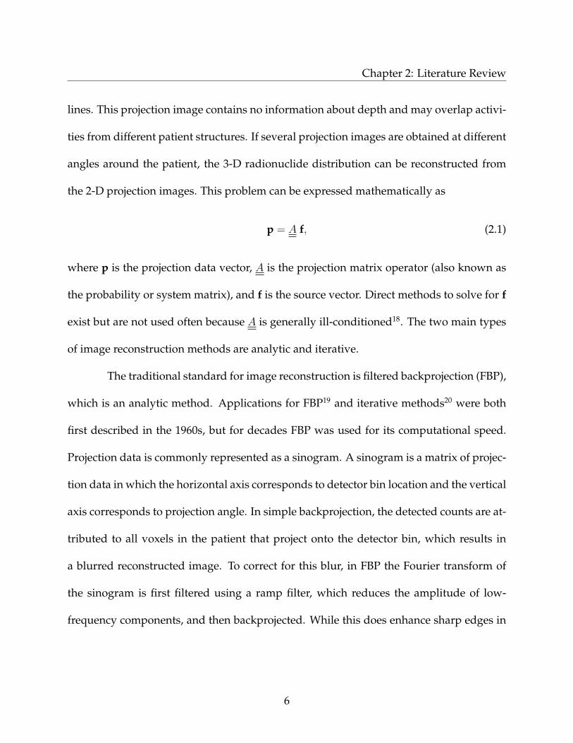
the 2-D projection images. This problem can be expressed mathematically as
p = A f, (2.1)
where p is the projection data vector, A is the projection matrix operator (also known as
the probability or system matrix), and f is the source vector. Direct methods to solve for f
exist but are not used often because A is generally ill-conditioned18. The two main types
of image reconstruction methods are analytic and iterative.
The traditional standard for image reconstruction is filtered backprojection (FBP),
which is an analytic method. Applications for FBP19 and iterative methods20 were both
first described in the 1960s, but for decades FBP was used for its computational speed.
Projection data is commonly represented as a sinogram. A sinogram is a matrix of projec-
tion data in which the horizontal axis corresponds to detector bin location and the vertical
axis corresponds to projection angle. In simple backprojection, the detected counts are at-
tributed to all voxels in the patient that project onto the detector bin, which results in
a blurred reconstructed image. To correct for this blur, in FBP the Fourier transform of
the sinogram is first filtered using a ramp filter, which reduces the amplitude of low-
frequency components, and then backprojected. While this does enhance sharp edges in
6

Chapter 2: Literature Review
the image, i.e., high-frequency components, it also enhances the high frequency noise.
Other filters can be used to help with this, but at the cost of spatial resolution.
Iterative reconstruction methods estimate the solution and compare the resulting
projections with the measured projections. Based on the comparison, the solution esti-
mate is then modified and the process is repeated. Each iterative reconstruction method
has a criterion for selecting the best solution and an algorithm to calculate it. Iterative re-
construction methods gained popularity during the 80s and 90s. While initially too time
consuming, as computer advances were made, these methods became more attractive. It-
erative reconstruction techniques are now primarily used instead of analytic reconstruc-
tion for emission tomography in the clinic16. Iterative reconstruction algorithms can be
grouped into constraint-based and statistical reconstruction techniques.
The algebraic reconstruction technique (ART)21 (also known as the Kaczmarz
method) is what constraint-based methods are generally known as. In the basic addi-
tive form of ART, Eq. 2.2, a new estimate of the source distribution is found by adding a
correction term to the current estimate.
f(k+1)j = f
(k)j +
pi −∑N
j=1 f(k)ji
N(2.2)
In Eq. 2.2, pi is the projection data along ray i, f (k)j and f
(k+1)j are the current and new
estimates, and∑N
j=1 f(k)ji is the sum of the counts along ray i. Note that one projection ray
at a time is considered and the correction term is the difference between the measured
projection and the current estimate. There are many different versions of ART algorithms,
7
Chapter 2: Literature Review
e.g., simultaneous iterative reconstruction technique (SIRT)22 and multiplicative algebraic
reconstruction technique (MART)21.
Statistical reconstruction methods are currently the most popular for emission to-
mography and of these the maximum likelihood expectation maximization23, 24 (ML-EM)
and ordered subsets expectation maximization25 (OS-EM) algorithms dominate26. The
ML-EM algorithm seeks to maximize the probability that a source distribution would
result in the observed projection images. OS-EM is an accelerated ML-EM algorithm in
which the projections are divided into subsets and a full iteration is complete once all sub-
sets are done. One subset is used for each sub-iteration so that fewer forward projections
are required for each full iteration. This reduces reconstruction time by approximately
the number of subsets while giving comparable image quality to ML-EM.
Like analytic methods, iterative reconstruction techniques have both advantages
and disadvantages. One advantage of ML-EM algorithms is the use of Poisson statis-
tics. The raw data obtained from SPECT contains Poisson noise and the inclusion of the
Poisson nature of SPECT projection data allows iterative reconstruction to perform better
than analytical algorithms in low count situations27. Iterative reconstruction methods also
allow for improved modeling of the image acquisition process. Disadvantages include in-
creasing noise for a high number of iterations, possible position-dependent convergence
rates, and long calculation times.
8

Chapter 2: Literature Review
2.3 SPECT Simulation and Reconstruction Codes
While there has been much research involving the simulation of SPECT, the focus
has been primarily on Monte Carlo methods. Several Monte Carlo codes have been
specifically designed to simulate SPECT, including GATE28, SimSPECT29, SimSET30, and
SIMIND31. GATE (Geant4 Application for Tomographic Emission) is based on the
Geant432 software toolkit for the simulation of the passage of particles through matter
and supports Positron Emission Tomography (PET), SPECT, CT, and radiotherapy exper-
iment simulations. SimSPECT is based on the MCNP33 Monte Carlo code. SIMIND was
developed by Professor Michael Ljungberg and describes a standard clinical SPECT cam-
era. Codes optimized for specific simulations, e.g., SIMIND, have the advantage of being
much faster; however, they may also be difficult to modify or give limited output, e.g.,
SIMIND does not give uncertainties at this time.
Others have developed complex analytical methods based on the Klein-Nishina
scatter equations for SPECT simulation34, 35. These methods usually are restricted in the
scattering order and geometry detail that can be modeled.
There are also some codes available for SPECT image reconstruction. Mathwork’s
MATLAB includes a FBP function and the Image Reconstruction Toolbox36 for MATLAB
includes FBP, ML-EM, and OS-EM algorithms. The QSPECT open-source software37 was
designed to provide a freely available application that includes the standard ML-EM and
OS-EM reconstruction algorithms and a system matrix calculation. STIR (Software for
Tomographic Image Reconstruction)38 is an open-source object-oriented library for PET
9
Chapter 2: Literature Review
image reconstruction that has recently been extended to SPECT39. GPU-accelerated recon-
struction tools for emission and transmission computed tomography are available with
NiftyRec40, which has MATLAB and Python interfaces.
2.4 Iterative Reconstruction Research
Iterative reconstruction techniques have overtaken FBP as the most popular technique in
the clinic for emission tomography, but there is still plenty of room for their improve-
ment. Current research in iterative image reconstruction emphasizes the optimization of
algorithms while improving the accuracy of the models incorporated into them26. The ap-
plication of iterative reconstruction algorithms to CT, for which FBP is still the preferred
algorithm, is under active investigation41. There is also ongoing research into solving for
motion during reconstruction, as well as simultaneous reconstruction of both the emis-
sion and attenuation distributions from emission data only. Consistent procedures for
evaluating the wide variety of reconstruction algorithms are needed to help move re-
search into the clinic and this is therefore an important area of development.
The noise in statistical methods increases with each iteration due to the noisy
projection data and early stopping or post-reconstruction smoothing is frequently used
to control this. Clearly, stopping at a lower number of iterations is not ideal since not all
of the image volume may have converged. Smoothing can result in a loss of resolution,
but is widely available and well understood. Bayesian algorithms have been used to
introduce a ’prior’ term in the maximum a-posteriori (MAP) algorithm using a one-step-
10
Chapter 2: Literature Review
late process42 that very closely resembles the ML-EM algorithm. The algorithm has an
additional term to penalize noise and current research seeks to optimize the penalty term
and its weighting constant26.
In making the models more exact, the modeling of scatter is a particularly active
area of research. If only attenuation is considered during reconstruction, i.e., projections
are assumed to contain uncollided particles only, the activity distribution in the patient is
over-estimated because the scatter counts contribute to the measured projections. Scatter
causes blurring in projections, reduces contrast, and increases quantification uncertainty.
However, a recent review by Hutton et al found that only basic scatter correction methods
have made it into regular usage43. All methods must balance making a more exact model
against increased computation time.
Incorporating scatter correction into reconstruction can be achieved by taking
measurements, modeling the scatter, or a combination of both. The most common mea-
surement-based scatter correction methods involve using narrow energy windows to esti-
mate the scatter. Recently much development has been seen in modeling scatter with the
help of advances in computing. Studies have shown improvement for accurate model-
ing of scatter over energy window-based scatter correction methods44, 45. Modeling does
have the disadvantage of not including contributions from activity located outside of the
reconstructed volume, e.g., the liver in cardiac imaging, but this issue is being worked
on46. Methods have been developed that use scatter functions created from experimental
measurements or Monte Carlo simulations of a slab of water and these were extended
11
Chapter 2: Literature Review
into the effective scatter source estimation (ESSE)47. Good results have been seen with the
ESSE method, but it does neglect photon transport from the source to the point of scatter.
Full Monte Carlo simulation of patient scatter has recently become possible for iterative
image reconstruction with the development of optimization methods48. One of these opti-
mizations is convolution forced detection (CFD), which significantly reduces the number
of photon histories necessary to produce a low-noise simulation49.
The ML-EM algorithm can be viewed as a series of ”forward” projections and
backprojections. In dual matrix ML-EM reconstruction, less detail is modeled in the back-
projection than in the forward projection to reduce computation time. Modeling scatter in
the forward projection only has been shown to give nearly the same signal-to-noise prop-
erties as including the scatter model in the backprojection step as well44. Zeng and Gull-
berg investigated the theoretical implications of using mismatched projectors and con-
ducted studies50. They concluded that, while theoretically a valid backprojector should
be chosen based on their criteria, in practical applications with noise present the choice of
a valid backprojector is not crucial and initial convergent behavior with a method to stop
the iteration process is more important.
In a review of the literature, no mention was found of the use of a deterministic
code to solve the linear Boltzmann equation, with the analytic models being the closest
comparison. Hutton et al comment that if accurate scatter models can be directly inte-
grated into reconstruction the range of photon energies used could be widened and result
in an improvement in the signal-to-noise ratio43.
12
Chapter 3
Theory
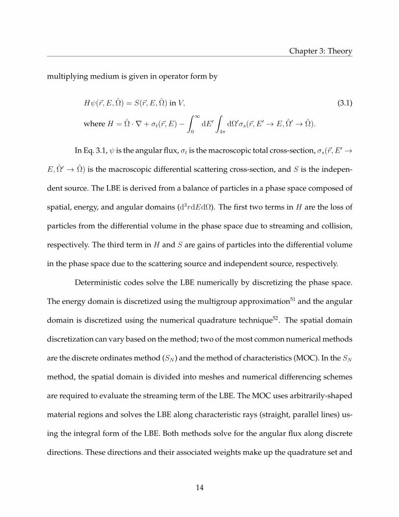
Here, the theory pertaining to this work is discussed. The linear Boltzmann equation is
described, the theory behind the TITAN code system is given with emphasis on pertinent
features, the ML-EM reconstruction algorithm is explained, and a novel deterministic
reconstruction methodology is introduced.
3.1 Solving the Linear Boltzmann Equation
The linear Boltzmann equation (LBE), also known as the transport equation, describes
neutral particles in a system and is derived from the Boltzmann equation with the
assumption that particle-particle interactions are negligible relative to particle-nucleus
interactions. The time-independent integro-differential form of the LBE for a non-
13
Chapter 3: Theory
multiplying medium is given in operator form by
Hψ(~r, E, Ω) = S(~r, E, Ω) in V, (3.1)
where H = Ω · ∇+ σt(~r, E)−∫ ∞
0
dE ′∫
4π
dΩ′σs(~r, E′ → E, Ω′ → Ω).
In Eq. 3.1, ψ is the angular flux, σt is the macroscopic total cross-section, σs(~r, E ′ →
E, Ω′ → Ω) is the macroscopic differential scattering cross-section, and S is the indepen-
dent source. The LBE is derived from a balance of particles in a phase space composed of
spatial, energy, and angular domains (d3rdEdΩ). The first two terms in H are the loss of
particles from the differential volume in the phase space due to streaming and collision,
respectively. The third term in H and S are gains of particles into the differential volume
in the phase space due to the scattering source and independent source, respectively.
Deterministic codes solve the LBE numerically by discretizing the phase space.
The energy domain is discretized using the multigroup approximation51 and the angular
domain is discretized using the numerical quadrature technique52. The spatial domain
discretization can vary based on the method; two of the most common numerical methods
are the discrete ordinates method (SN ) and the method of characteristics (MOC). In the SN
method, the spatial domain is divided into meshes and numerical differencing schemes
are required to evaluate the streaming term of the LBE. The MOC uses arbitrarily-shaped
material regions and solves the LBE along characteristic rays (straight, parallel lines) us-
ing the integral form of the LBE. Both methods solve for the angular flux along discrete
directions. These directions and their associated weights make up the quadrature set and
14
Chapter 3: Theory
(a) S10 (120 directions)
(b) S20 (440 directions)
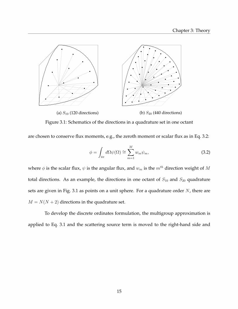
Figure 3.1: Schematics of the directions in a quadrature set in one octant
are chosen to conserve flux moments, e.g., the zeroth moment or scalar flux as in Eq. 3.2:
φ =
∫4π
dΩψ(Ω) ∼=M∑m=1
wmψm, (3.2)
where φ is the scalar flux, ψ is the angular flux, and wm is the mth direction weight of M
total directions. As an example, the directions in one octant of S10 and S20 quadrature
sets are given in Fig. 3.1 as points on a unit sphere. For a quadrature order N , there are
M = N(N + 2) directions in the quadrature set.
To develop the discrete ordinates formulation, the multigroup approximation is
applied to Eq. 3.1 and the scattering source term is moved to the right-hand side and
15
Chapter 3: Theory
written in terms of spherical harmonics to give the formulation of the LBE in Eq. 3.3.
(µ∂
∂x+ η
∂
∂y+ ξ
∂
∂z
)ψg(x, y, z, µ, ϕ) + σg(x, y, z)ψg(x, y, z, µ, ϕ) =
G∑g′=1
L∑l=0
(2l + 1)σs,g′→g,l(x, y, z)
Pl(µ)φg′,l(x, y, z)+ (3.3)
2l∑
k=1
(l − k)!
(l + k)!P kl (µ)×
[φkCg′,l(x, y, z)cos(kϕ) + φkSg′,l(x, y, z)sin(kϕ)
]+
Sg(x, y, z, µ, ϕ)
In Eq. 3.3, θ and ϕ are the polar and azimuthal angles, respectively, and a discrete ordinate
is specified by (θ, ϕ) or (µ, η, ξ), where µ = cos(θ), η = sin(θ)cos(ϕ), and ξ = sin(θ)sin(ϕ).
Pl(µ) is the lth Legendre polynomial and L is the Legendre expansion order. P kl (µ) is the
lth, kth associated Legendre polynomial. ψg(x, y, z, µ, ϕ) is the group g angular flux, G is
the total number of energy groups, σg is the group macroscopic total cross-section, σs,g′→g,l
is the lth moment of the macroscopic differential scattering cross-section from group g′ to
g, and Sg is the independent fixed source. The flux moments are defined by
φg′,l(x, y, z) =
∫ 1
−1
dµ′
2Pl(µ
′)
∫ 2π
0
dϕ′
2πψg′(x, y, z, µ
′, ϕ′) (3.4)
φkCg′,l(x, y, z) =
∫ 1
−1
dµ′
2P kl (µ′)
∫ 2π
0
dϕ′
2πcos(kϕ′)ψg′(x, y, z, µ
′, ϕ′) (3.5)
φkSg′,l(x, y, z) =
∫ 1
−1
dµ′
2P kl (µ′)
∫ 2π
0
dϕ′
2πsin(kϕ′)ψg′(x, y, z, µ
′, ϕ′), (3.6)
where φg′,l is the lth Legendre flux moment for group g′, φkCg′,l is the lth, kth cosine associ-
ated Legendre flux moment for group g′, and φkSg′,l is the lth, kth sine associated Legendre
16

Chapter 3: Theory
flux moment for group g′. Eq. 3.3 has energy and angular discretization since the angular
flux is solved for energy group g in discrete directions (µn, φn) from the quadrature set of
N total directions.
The spatial variable is discretized using the finite volume method52 by integrating
Eq. 3.3 over the fine mesh volume Vijk = ∆x∆y∆z to form
µn∆x
(ψx,out − ψx,in) +ηn∆y
(ψy,out − ψy,in) +ξn∆z
(ψz,out − ψz,in) + σijkψ(n)gijk = Q
(n)gijk, (3.7)
where Q(n)gijk = S
(n)scat,gijk+S
(n)gijk. In Eq. 3.7, ψx,in, ψy,in, and ψz,in are the angular fluxes on the
incoming boundaries of the fine mesh and ψx,out, ψy,out, and ψz,out are the angular fluxes on
the outgoing boundaries. ψ(n)gijk is the average angular flux in fine mesh ijk along direction
n for group g and Q(n)gijk is the average angular source.
While the differential is removed, there are now additional unknowns in Eq. 3.7.
The three incoming fluxes are obtained from boundary conditions and so three additional
equations are needed to solve for ψ(n)gijk. These additional equations are provided by the
chosen differencing scheme. The linear diamond differencing (DD) scheme is one of the
simplest and is given by
ψx,out = 2ψx,in − ψ(n)gijk,
ψy,out = 2ψy,in − ψ(n)gijk, (3.8)
and ψz,out = 2ψz,in − ψ(n)gijk.
17
Chapter 3: Theory
The DD scheme assumes that the average flux is given by a linear average of the boundary
fluxes. However, the DD scheme can give negative fluxes and for this reason is usually
implemented with the zero fix-up approach and referred to as the DDZ scheme.
The LBE can be solved using the source iteration method. The source Q is cal-
culated from the last iteration’s results and taken as a constant while solving Eq. 3.7 for
the angular flux ψ. The flux moments are then obtained from Eqs. 3.4-3.6 and used to up-
date the source Q for the next iteration. This process is repeated until some convergence
criterion is met, generally convergence of the 0th flux moment, i.e., the scalar flux.
Deterministic methods can have numerical issues that lead to what are referred
to as ray effects and unphysical oscillations. In situations with localized sources and little
scatter, the uncollided flux is dominant and deterministic methods can result in oscilla-
tions in the scalar flux that are called ray effects52. Ray effects arise when the quadrature
set cannot adequately approximate the scalar flux from the angular flux, as in Eq. 3.2.
The simplest solution is to increase the quadrature order, i.e., the number of directions.
Unphysical oscillations arise at source discontinuities from the differencing scheme not
taking particle direction into account when obtaining coefficients for each axis53.
As briefly mentioned earlier, the MOC is another popular method for solving the
LBE. Unlike, the SN formulation, the MOC can represent the model geometry exactly by
filling arbitrarily shaped regions with characteristic rays along the directions of a quadra-
ture set. The LBE along characteristic ray k in region i, energy group g, and direction n is
18

Chapter 3: Theory
given by
dψ(n)gik(l)
dl+ σgiψ
(n)gik(l) = Q
(n)gi . (3.9)
In Eq. 3.9, l is the path length along characteristic ray k and constant cross sections and
source are assumed within a region. If the incoming angular flux is known, Eq. 3.9 can be
solved analytically. The angular flux out of region i is then calculated by
ψ(n)gik,out = ψ
(n)gik(s
(n)ik ) = ψ
(n)gik,ine
−σgis(n)ik +
Q(n)gi
σgi
(1− e−σgis
(n)ik
), (3.10)
where s(n)ik is the path length of ray k. For each region, the average angular flux is found by
filling the region with characteristic rays along the quadrature set directions and taking
a weighted average. The source iteration method can also be used with the MOC. To get
accurate results, the flux must change slowly over the region and enough characteristic
rays must be modeled to cover the region. The MOC method is also susceptible to ray
effects, but is numerically more efficient in low scatter regions4.
3.2 The TITAN Code
3.2.1 Hybrid Formulation
The TITAN code is a hybrid deterministic transport code that numerically solves the lin-
ear Boltzmann equation (LBE) for neutral particles54. The source iteration method de-
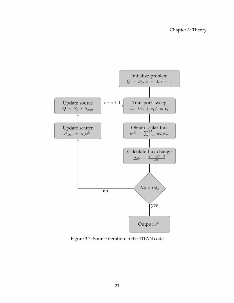
scribed in Section 3.1 is implemented in TITAN as shown in Fig. 3.2 for a single energy
19
Chapter 3: Theory
group and fixed source S0. The transport sweep solves for the angular flux distribution,
which is then used to obtain the scalar flux and calculate the flux moments. The flux mo-
ments are used to update the scattering source Sscat and add it to the total source Q and
the process is then repeated.
The TITAN code is a “hybrid” code because it allows the use of different solvers
in the spatial domain with its multi-block framework. In different regions (called coarse
meshes) of a problem, the user can specify a discrete ordinates52 (SN ) solver or a character-
istics method55 (CM) solver. There are two differencing schemes available in the TITAN
code: diamond differencing with zero fix-up (DDZ) and directional theta-weighted
(DTW)56. The CM discretizes the angular domain as in the SN method, but instead of
using spatial meshes, the integral form of the LBE is used to calculate the angular flux
along parallel directions called characteristic rays. The CM does not require the use of a
differencing scheme, but still can be memory intensive because of the need for a large set
of characteristic rays.
3.2.2 Parallel Implementation
Parallel performance has become a vital attribute of modern algorithms in order for them
to be applied to real-world problems. The TITAN code is parallelized by angular de-
composition of individual ordinates, i.e., directions, in that each processor is assigned a
set of ordinates and stores only those ordinates to partition memory. In each iteration
in Fig. 3.2, a transport sweep is performed on each processor for its set of ordinates and
20
Chapter 3: Theory
Initialize problemQ = S0, φ = 0, i = 1
Transport sweepΩ · ∇ψ + σtψ = Q
Obtain scalar fluxφ(i) =
∑Mm=1wmψm
Calculate flux change∆φ = φ(i)−φ(i−1)
φ(i)
∆φ < tolφ
Output φ(i)
Update scatterSscat = σsφ
(i)
Update sourceQ = S0 + Sscat
no
yes
i = i+ 1
Figure 3.2: Source iteration in the TITAN code
21
Chapter 3: Theory
the corresponding flux moments are calculated. At the end of the iteration, all proces-
sors communicate using MPI (Message Passing Interface) and the flux moments from all
subsets are combined to get the total flux moments. If reflective boundary conditions
are present, the number of processors is limited to the number of ordinates per octant,
Fig. 3.1, so that all possible reflections of an ordinate to another octant are stored on the
same processor. This allows reflective boundary conditions to be applied without any
additional communication.
3.2.3 SPECT Formulation
To simulate SPECT, the TITAN code uses a four step hybrid SN and simplified ray-tracing
formulation57:
1. SN transport calculation in the phantom, or patient, with a regular quadrature set
2. Generation of fictitious quadrature set57 with circular ordinate splitting for a projec-
tion angle
3. One extra transport sweep in the phantom with the fictitious quadrature set using
the converged flux moments from Step 1 to evaluate the scattering source
4. Simulation of the projection image with the fictitious quadrature set using the sim-
plified ray-tracing formulation outside of the phantom.
Step 1 only needs to be completed once and Steps 2-4 are then repeated for each projection
angle desired. Each voxel of the phantom is modeled as a fine mesh in TITAN. In Step
22
Chapter 3: Theory
2, the fictitious quadrature set is created to represent the projection directions needed for
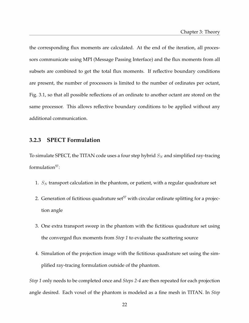
a specific SPECT projection image. Fig. 3.3 demonstrates a fictitious quadrature set with
forty projection angles and eight split directions per projection angle.
Figure 3.3: Example schematic of a fictitious quadrature setwith circular ordinate splitting.
The ordinate splitting technique58 was adapted in the TITAN code for use in sim-
ulating the collimator in SPECT to create the circular ordinate splitting (COS) technique.
It is not reasonable to directly model the SPECT collimator due to the fine spatial and
angular discretization that would be required. The COS technique is used to represent an
acceptance angle about the detector normal within which incoming photons will reach
the detector without interacting with the collimator. In the COS technique, split direc-
tions are made on a circle, or concentric circles, centered on the original projection direc-
tion, as depicted in Figs. 3.3 and 3.4. The radius of the outermost circle is chosen to match
the desired collimator acceptance angle. The angular fluxes over the original and split
directions are averaged to simulate the flux passing through the collimator.
The fictitious quadrature set is created to calculate the angular fluxes for certain
directions and does not require flux moments to be conserved as in a regular quadrature
23
Chapter 3: Theory
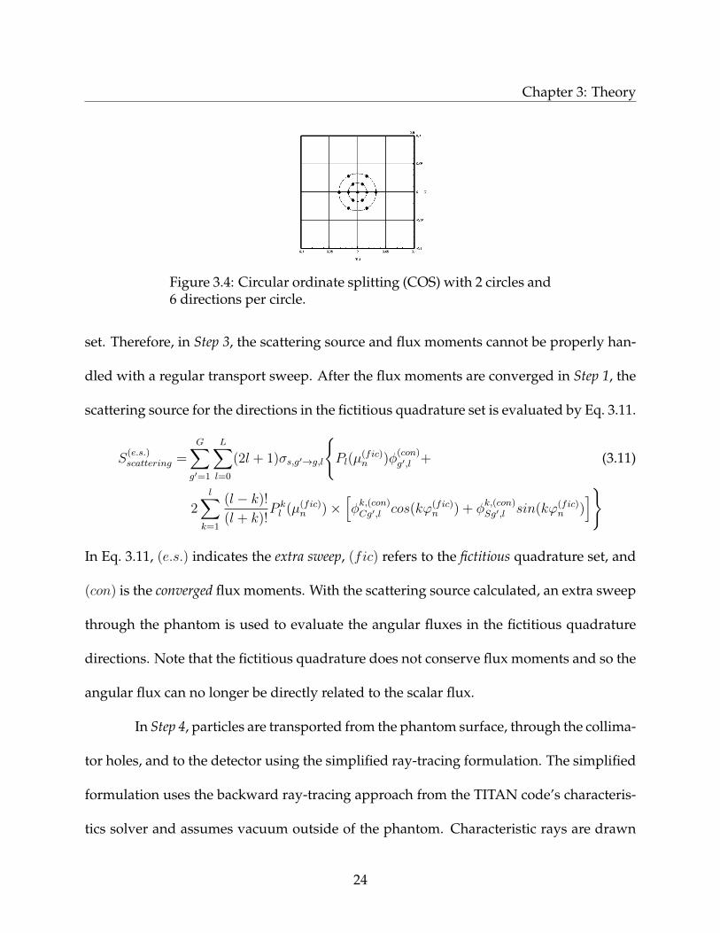
Figure 3.4: Circular ordinate splitting (COS) with 2 circles and6 directions per circle.
set. Therefore, in Step 3, the scattering source and flux moments cannot be properly han-
dled with a regular transport sweep. After the flux moments are converged in Step 1, the
scattering source for the directions in the fictitious quadrature set is evaluated by Eq. 3.11.
S(e.s.)scattering =
G∑g′=1
L∑l=0
(2l + 1)σs,g′→g,l
Pl(µ
(fic)n )φ
(con)g′,l + (3.11)
2l∑
k=1
(l − k)!
(l + k)!P kl (µ(fic)
n )×[φk,(con)Cg′,l cos(kϕ(fic)
n ) + φk,(con)Sg′,l sin(kϕ(fic)
n )]
In Eq. 3.11, (e.s.) indicates the extra sweep, (fic) refers to the fictitious quadrature set, and
(con) is the converged flux moments. With the scattering source calculated, an extra sweep
through the phantom is used to evaluate the angular fluxes in the fictitious quadrature
directions. Note that the fictitious quadrature does not conserve flux moments and so the
angular flux can no longer be directly related to the scalar flux.
In Step 4, particles are transported from the phantom surface, through the collima-
tor holes, and to the detector using the simplified ray-tracing formulation. The simplified
formulation uses the backward ray-tracing approach from the TITAN code’s characteris-
tics solver and assumes vacuum outside of the phantom. Characteristic rays are drawn
24

Chapter 3: Theory
from each image pixel backward to the phantom surface along the projection angle and
the split directions. Where a ray intersects with the phantom surface, the angular flux has
already been calculated for the direction in Step 3 and a bi-linear interpolation is used to
evaluate the angular flux at that intersection point.
3.3 ML-EM Reconstruction
The simplified derivation of the maximum likelihood expectation maximization (ML-EM)
formulation that follows is based on Bruyant’s explanation in ref. 18. The ML-EM algo-
rithm assumes that the number of emitted particles and detected particles are both Pois-
son random variables. Therefore the probability of detecting k counts in detector bin d
is
P (nd = k) = e−ndnkdk!, (3.12)
where nd is the mean number of photons detected in bin d given by
nd =B∑b=1
pb,dλb. (3.13)
In Eq. 3.13, pb,d is the probability that a photon emitted from voxel b is detected in detector
bin d and λb is the mean number of emissions in voxel b for b = 1, . . . , B voxels and
d = 1, . . . , D bins.
The likelihood, L(λ), is the conditional probability P (n|λ) of observing n if the
emission rate is λ. For D detector bins, the Poisson variables are independent and so the
conditional probability is the product of the individual probabilities. Using Eq. 3.12, the
25
Chapter 3: Theory
likelihood function is given by
L(λ) = P (n|λ) =D∏d=1
P (nd)
=D∏d=1
e−ndnndd
nd!. (3.14)
At this point, the natural logarithm of the likelihood function is taken to simplify the
derivation. Recalling that ln(x1x2 . . . xn) = ln(x1) + ln(x2) + · · ·+ ln(xn), the log-likelihood
can be simplified to
l(λ) = ln(L(λ)) =D∑d=1
ln
(e−nd
nndd
nd!
)
=D∑d=1
[−nd + nd ln(nd)− ln(nd!)] . (3.15)
Eq. 3.13 is now substituted into Eq. 3.15 to give
l(λ) =D∑d=1
[−
B∑b=1
pb,dλb + nd ln(B∑b=1
pb,dλb)− ln(nd!)
]. (3.16)
Eq. 3.16 is the probability of observing a projection dataset n for mean image λ. The goal
is to obtain the image that is most likely to produce n by finding the image λ for which
l(λ) is maximized. To find this maximum, the derivative of l(λ) is set to zero:
∂l(λ)
∂λb= −
D∑d=1
pb,d +D∑d=1
nd∑Bb′=1 pb′,dλb′
pb,d = 0. (3.17)
Multiplying Eq. 3.17 by λb gives
−λbD∑d=1
pb,d + λb
D∑d=1
nd∑Bb′=1 pb′,dλb′
pb,d = 0, (3.18)
26

Chapter 3: Theory
which can then be rearranged to form
λb =λb∑Dd=1 pb,d
D∑d=1
nd∑Bb′=1 pb′,dλb′
pb,d. (3.19)
Eq. 3.19 can be modified to give the iterative form of the ML-EM algorithm
λ(i+1)b =
λ(i)b∑D
d=1 pb,d
D∑d=1
n∗dpb,d∑Bb′=1 λ
(i)b′ pb′,d
, b = 1, . . . , B, (3.20)
where λ(i)b is the estimate of the unknown emission density in voxel b for iteration i, n∗d
is the measured data in detector pixel d, and pb,d is the probability or system matrix and
gives the probability that an emission in voxel b is detected in detector pixel d.
3.4 Novel Deterministic Reconstruction Methodology
The ML-EM iterative algorithm given in Eq. 3.20 can be viewed as a series of projections
and backprojections. The denominator∑B
b′=1 λ(i)b′ pb′,d is the projection of the current image
estimate. Eq. 3.20 can then be rewritten as
λ(i+1)b =
λ(i)b∑D
d=1 pb,d
D∑d=1
n∗d
n(i)d
pb,d, b = 1, . . . , B, (3.21)
where n(i)d is the projection of the current estimate. The ratio of the measured projection
data to the projection estimate is then backprojected so that Eq. 3.21 can be simplified into
Eq. 3.2218.
Emission(i+1) = Emission(i) ×Backprojection of(Measured Projections
Estimated Projections
)(3.22)
27

Chapter 3: Theory
A deterministic code that generates projection images can then be used to provide the
estimated projections. This methodology is referred to here as deterministic reconstruc-
tion for SPECT (DRS) and was developed to take advantage of the TITAN code’s fast
algorithm for simulating SPECT projection images.
DRS can be viewed as a modified version of dual matrix image reconstruction,
in which different system matrices are used for the projection and backprojection steps.
Dual matrix image reconstruction allows for the backprojection system matrix to model
less detail than the ”forward” projection system matrix to reduce reconstruction time. The
system matrix can model attenuation, depth-dependent collimator response, and even
scatter, but can become difficult to compute and prohibitively large with the addition of
this detail. In DRS, a single system matrix is not used for projection and backprojection,
but unlike dual matrix reconstruction only the simpler backprojection system matrix is
needed. The deterministic code completes the projection step and is able to fully model
particle transport, including scatter, in the patient or phantom without the need of a com-
plicated system matrix.
28

Chapter 4
Analysis of SPECT Algorithm in TITAN
Studies were conducted to analyze the TITAN code for SPECT simulation before applying
it to image reconstruction. TITAN projection images are compared with results from the
SIMIND code, the MCNP5 code, and an experiment.
This work focuses on simulating a myocardial perfusion study using Technetium-
99m (Tc-99m) and so a 140 keV photon source is used. Three-group multigroup cross
sections generated using the CEPXS code59 were used. The first energy group is 126.45-
154.55 keV to account for a typical energy window of 20% and is the group of interest.
The second energy group is 126.45-154.55 keV and the third is 10-126.45 keV. Projection
images are normalized to the highest value pixel before comparison.
29
Chapter 4: Analysis of SPECT Algorithm in TITAN
4.1 Projection Comparison with SIMIND
SPECT projection images generated by TITAN were compared with the SIMIND Monte
Carlo code60. The NURBS-based cardiac-torso (NCAT) code61 was used to generate a
64× 64× 64 voxel phantom (0.625× 0.625× 0.625 cm3 voxel size) for use in both SIMIND
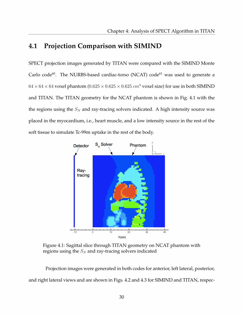
and TITAN. The TITAN geometry for the NCAT phantom is shown in Fig. 4.1 with the
the regions using the SN and ray-tracing solvers indicated. A high intensity source was
placed in the myocardium, i.e., heart muscle, and a low intensity source in the rest of the
soft tissue to simulate Tc-99m uptake in the rest of the body.
Figure 4.1: Sagittal slice through TITAN geometry on NCAT phantom withregions using the SN and ray-tracing solvers indicated
Projection images were generated in both codes for anterior, left lateral, posterior,
and right lateral views and are shown in Figs. 4.2 and 4.3 for SIMIND and TITAN, respec-
30
Chapter 4: Analysis of SPECT Algorithm in TITAN
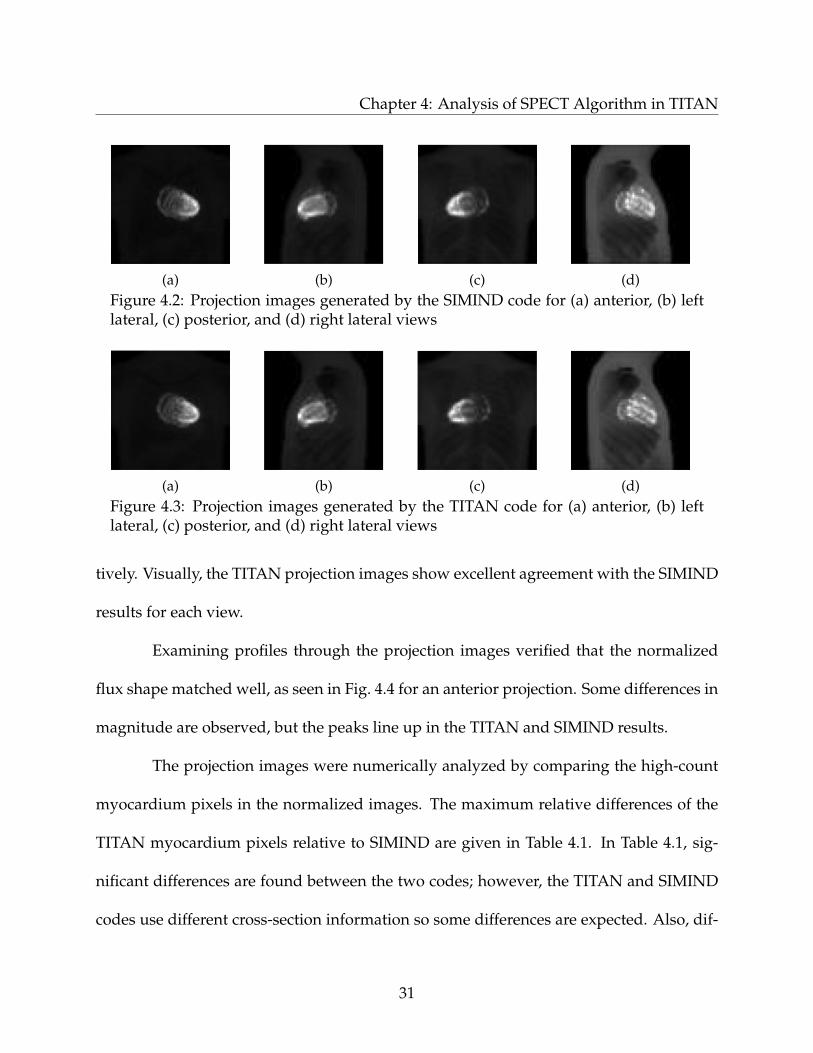
(a) (b) (c) (d)Figure 4.2: Projection images generated by the SIMIND code for (a) anterior, (b) leftlateral, (c) posterior, and (d) right lateral views
(a) (b) (c) (d)Figure 4.3: Projection images generated by the TITAN code for (a) anterior, (b) leftlateral, (c) posterior, and (d) right lateral views
tively. Visually, the TITAN projection images show excellent agreement with the SIMIND
results for each view.
Examining profiles through the projection images verified that the normalized
flux shape matched well, as seen in Fig. 4.4 for an anterior projection. Some differences in
magnitude are observed, but the peaks line up in the TITAN and SIMIND results.
The projection images were numerically analyzed by comparing the high-count
myocardium pixels in the normalized images. The maximum relative differences of the
TITAN myocardium pixels relative to SIMIND are given in Table 4.1. In Table 4.1, sig-
nificant differences are found between the two codes; however, the TITAN and SIMIND
codes use different cross-section information so some differences are expected. Also, dif-
31

Chapter 4: Analysis of SPECT Algorithm in TITAN
0 0.1 0.2 0.3 0.4 0.5 0.6 0.7 0.8 0.9
1
20 25 30 35 40 45 50
Nor
mal
ized
Flu
x
Projection Image Pixel Number
Anterior Projection Image Column 44 Flux
TITAN SIMIND
(a)
0 0.1 0.2 0.3 0.4 0.5 0.6 0.7 0.8 0.9
1
20 25 30 35 40 45 50
Nor
mal
ized
Flu
x
Projection Image Pixel Number
Anterior Projection Image Row 38 Flux
TITAN
SIMIND
(b)Figure 4.4: (a) Vertical and (b) horizontal profiles through heart in anterior projectionsfrom TITAN and SIMIND.
ferent methods of representing collimation are used by the two codes. It is interesting
to note that the largest relative differences are seen for the projection angles where the
heart is deepest in the phantom. The SIMIND code has the user select a fixed number of
photons to simulate per projection angle. This will result in fewer photons reaching the
detector for the posterior and right lateral projections and therefore larger uncertainties
in a Monte Carlo code like SIMIND.
Table 4.1: Maximum difference of TITAN results relative toSIMIND results for each projection
Anterior Left Lateral Posterior Right Lateral
16.4% -12.8% -23.5% -25.8%
The computation times of the SIMIND and TITAN codes for different numbers of
projection angles on a single processor are compared in Table 4.2. The speed of the spe-
cialized SIMIND code is apparent for small numbers of projections; however, for the large
numbers of projections that would be necessary for image reconstruction, the TITAN code
shows a clear advantage over the SIMIND code. Recall from Section 3.2 that to simulate
32
Chapter 4: Analysis of SPECT Algorithm in TITAN
SPECT projection images, TITAN completes the time-consuming phantom flux calcula-
tion once and is then able to generate the projection images at each angle with little addi-
tional computational cost. In contrast, the SIMIND code completes each projection angle
calculation separately. The SIMIND results presented here used one million photons per
projection image, but the SIMIND code does not output any statistical information about
the solution. It is up to the user to verify that enough photons have been simulated and
this has been done by plotting the infinity-norm and 2-norm as a function of photons
simulated.
Table 4.2: SIMIND and TITAN computation times
Number of Projection Images 1 4 8 45 90
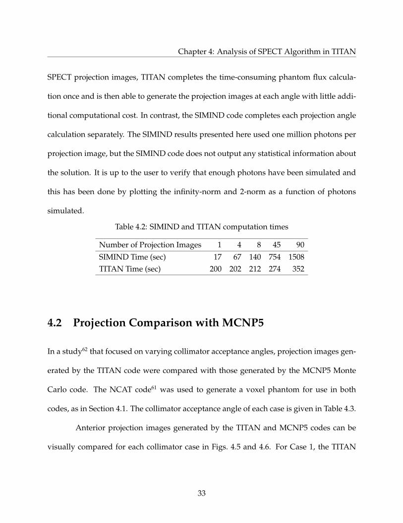
SIMIND Time (sec) 17 67 140 754 1508TITAN Time (sec) 200 202 212 274 352
4.2 Projection Comparison with MCNP5
In a study62 that focused on varying collimator acceptance angles, projection images gen-
erated by the TITAN code were compared with those generated by the MCNP5 Monte
Carlo code. The NCAT code61 was used to generate a voxel phantom for use in both
codes, as in Section 4.1. The collimator acceptance angle of each case is given in Table 4.3.
Anterior projection images generated by the TITAN and MCNP5 codes can be
visually compared for each collimator case in Figs. 4.5 and 4.6. For Case 1, the TITAN
33

Chapter 4: Analysis of SPECT Algorithm in TITAN
Table 4.3: Collimator cases with different acceptance angles
Case number Acceptance Angle
1 2.97
2 1.42
3 0.98
(a) Case 1 (b) Case 2 (c) Case 3
Figure 4.5: MCNP5 anterior projection images for collimator cases
(a) Case 1 (b) Case 2 (c) Case 3
Figure 4.6: TITAN anterior projection images for collimator cases
image, Fig. 4.6a, appears less blurred than the MCNP5 image, Fig. 4.5a. As expected, the
images become sharper as the acceptance angle decreases, i.e., the case number increases.
Table 4.4 gives the acceptance angle and maximum relative error in the heart
corresponding to each collimator case. In Table 4.4, it is clear that the differences between
the TITAN and MCNP5 projection images are reduced with decreasing acceptance angle.
34
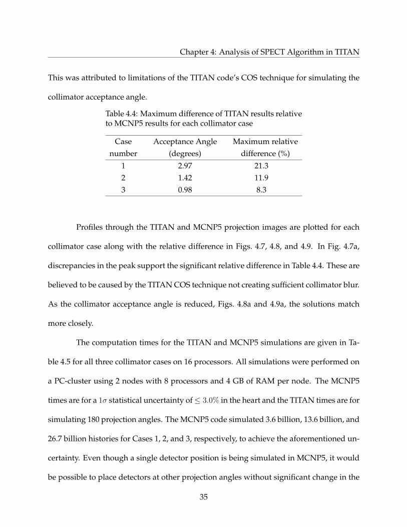
Chapter 4: Analysis of SPECT Algorithm in TITAN
This was attributed to limitations of the TITAN code’s COS technique for simulating the
collimator acceptance angle.
Table 4.4: Maximum difference of TITAN results relativeto MCNP5 results for each collimator case
Case Acceptance Angle Maximum relativenumber (degrees) difference (%)
1 2.97 21.32 1.42 11.93 0.98 8.3
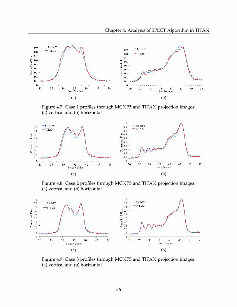
Profiles through the TITAN and MCNP5 projection images are plotted for each
collimator case along with the relative difference in Figs. 4.7, 4.8, and 4.9. In Fig. 4.7a,
discrepancies in the peak support the significant relative difference in Table 4.4. These are
believed to be caused by the TITAN COS technique not creating sufficient collimator blur.
As the collimator acceptance angle is reduced, Figs. 4.8a and 4.9a, the solutions match
more closely.
The computation times for the TITAN and MCNP5 simulations are given in Ta-
ble 4.5 for all three collimator cases on 16 processors. All simulations were performed on
a PC-cluster using 2 nodes with 8 processors and 4 GB of RAM per node. The MCNP5
times are for a 1σ statistical uncertainty of≤ 3.0% in the heart and the TITAN times are for
simulating 180 projection angles. The MCNP5 code simulated 3.6 billion, 13.6 billion, and
26.7 billion histories for Cases 1, 2, and 3, respectively, to achieve the aforementioned un-
certainty. Even though a single detector position is being simulated in MCNP5, it would
be possible to place detectors at other projection angles without significant change in the
35
Chapter 4: Analysis of SPECT Algorithm in TITAN
(a) (b)
Figure 4.7: Case 1 profiles through MCNP5 and TITAN projection images:(a) vertical and (b) horizontal
(a) (b)
Figure 4.8: Case 2 profiles through MCNP5 and TITAN projection images:(a) vertical and (b) horizontal
(a) (b)
Figure 4.9: Case 3 profiles through MCNP5 and TITAN projection images:(a) vertical and (b) horizontal
36
Chapter 4: Analysis of SPECT Algorithm in TITAN
calculation time. This is why 180 projection angles are being used in the TITAN simula-
tion for the computation time comparison with MCNP5.
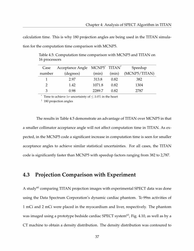
Table 4.5: Computation time comparison with MCNP5 and TITAN on16 processors
Case Acceptance Angle MCNP5* TITAN† Speedupnumber (degrees) (min) (min) (MCNP5/TITAN)
1 2.97 313.8 0.82 3822 1.42 1071.8 0.82 13043 0.98 2289.7 0.82 2787
* Time to achieve 1σ uncertainty of ≤ 3.0% in the heart† 180 projection angles
The results in Table 4.5 demonstrate an advantage of TITAN over MCNP5 in that
a smaller collimator acceptance angle will not affect computation time in TITAN. As ex-
pected, in the MCNP5 code a significant increase in computation time is seen for smaller
acceptance angles to achieve similar statistical uncertainties. For all cases, the TITAN
code is significantly faster than MCNP5 with speedup factors ranging from 382 to 2,787.
4.3 Projection Comparison with Experiment
A study60 comparing TITAN projection images with experimental SPECT data was done
using the Data Spectrum Corporation’s dynamic cardiac phantom. Tc-99m activities of
1 mCi and 2 mCi were placed in the myocardium and liver, respectively. The phantom
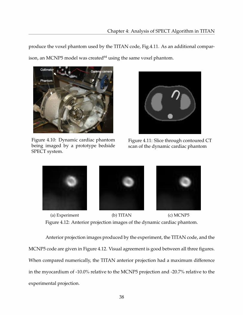
was imaged using a prototype bedside cardiac SPECT system63, Fig. 4.10, as well as by a
CT machine to obtain a density distribution. The density distribution was contoured to
37
Chapter 4: Analysis of SPECT Algorithm in TITAN
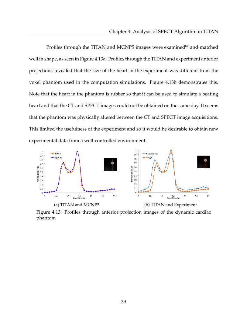
produce the voxel phantom used by the TITAN code, Fig.4.11. As an additional compar-
ison, an MCNP5 model was created64 using the same voxel phantom.
Figure 4.10: Dynamic cardiac phantombeing imaged by a prototype bedsideSPECT system.
Figure 4.11: Slice through contoured CTscan of the dynamic cardiac phantom
(a) Experiment (b) TITAN (c) MCNP5
Figure 4.12: Anterior projection images of the dynamic cardiac phantom.
Anterior projection images produced by the experiment, the TITAN code, and the
MCNP5 code are given in Figure 4.12. Visual agreement is good between all three figures.
When compared numerically, the TITAN anterior projection had a maximum difference
in the myocardium of -10.0% relative to the MCNP5 projection and -20.7% relative to the
experimental projection.
38
Chapter 4: Analysis of SPECT Algorithm in TITAN
Profiles through the TITAN and MCNP5 images were examined64 and matched
well in shape, as seen in Figure 4.13a. Profiles through the TITAN and experiment anterior
projections revealed that the size of the heart in the experiment was different from the
voxel phantom used in the computation simulations. Figure 4.13b demonstrates this.
Note that the heart in the phantom is rubber so that it can be used to simulate a beating
heart and that the CT and SPECT images could not be obtained on the same day. It seems
that the phantom was physically altered between the CT and SPECT image acquisitions.
This limited the usefulness of the experiment and so it would be desirable to obtain new
experimental data from a well-controlled environment.
(a) TITAN and MCNP5 (b) TITAN and Experiment
Figure 4.13: Profiles through anterior projection images of the dynamic cardiacphantom
39
Chapter 5
Enhancement of SPECT Algorithm in
TITAN
Two enhancements to the SPECT algorithm in TITAN are made in this section with re-
gard to computation time and accuracy. The parallel behavior of the SPECT algorithm
in TITAN is examined and improved. Based on the results of the collimator study in
Chapter 4, improvements are made to the collimator representation in TITAN.
5.1 Parallel Computation
5.1.1 Parallel Processing Metrics
The parallel speedup, parallel efficiency, and parallelizable fraction can be calculated to
give an indication of an algorithm’s parallel performance. The parallel speedup (SP ) is
40

Chapter 5: Enhancement of SPECT Algorithm in TITAN
defined as the ratio of the wall-clock time for a single processor (Ts) to the wall-clock time
in parallel. The parallel efficiency indicates the economic advantage of the parallelization
and is the parallel speedup divided by the number of processors (P ). Amdahl’s Law65
can be used to find the parallel fraction of a code by
SP =1
(1− fP ) + fP/P + Tc/Ts, (5.1)
where fP is the parallelizable fraction of the code and Tc is the parallel communication
time. If the parallel communication time is assumed to be much less than the serial com-
putation time, Eq. 5.1 can be rewritten as
fP =P (1− SP )
SP (1− P ). (5.2)
The parallelizable fraction in Eq. 5.2 gives a lower limit on the actual parallelizable
fraction.
Several factors impact and limit parallel performance. In the limit of infinite pro-
cessors (and zero communication time), Eq. 5.1 gives SP = 1/(1 − fP ). However, this
theoretical speedup will not be observed due to increasing communication overhead with
the addition of processors, i.e., more processors will eventually lead to low efficiency. The
load balance and granularity are also important to consider. Load balance refers to how
evenly the work is distributed among processors. Granularity refers to the number of
operations executed by processors before communication between them occurs.
41
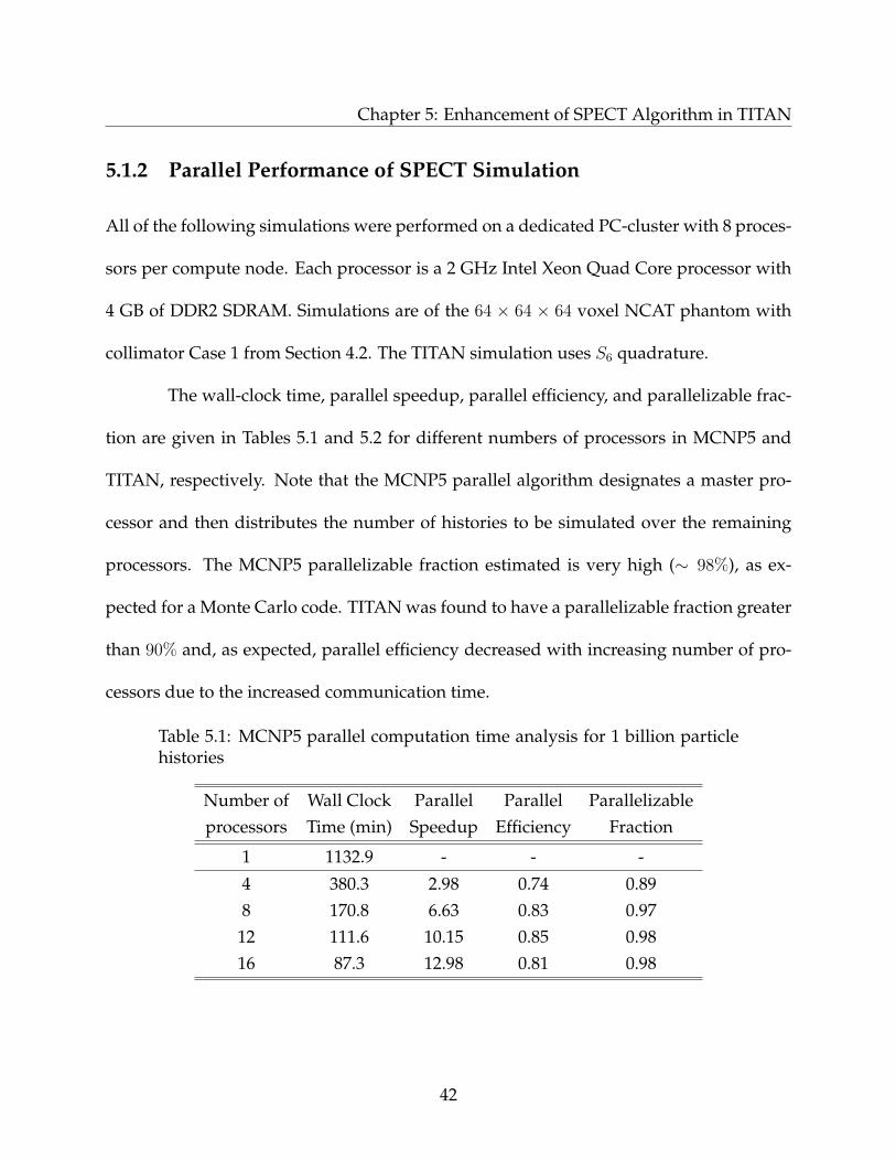
Chapter 5: Enhancement of SPECT Algorithm in TITAN
5.1.2 Parallel Performance of SPECT Simulation
All of the following simulations were performed on a dedicated PC-cluster with 8 proces-
sors per compute node. Each processor is a 2 GHz Intel Xeon Quad Core processor with
4 GB of DDR2 SDRAM. Simulations are of the 64 × 64 × 64 voxel NCAT phantom with
collimator Case 1 from Section 4.2. The TITAN simulation uses S6 quadrature.
The wall-clock time, parallel speedup, parallel efficiency, and parallelizable frac-
tion are given in Tables 5.1 and 5.2 for different numbers of processors in MCNP5 and
TITAN, respectively. Note that the MCNP5 parallel algorithm designates a master pro-
cessor and then distributes the number of histories to be simulated over the remaining
processors. The MCNP5 parallelizable fraction estimated is very high (∼ 98%), as ex-
pected for a Monte Carlo code. TITAN was found to have a parallelizable fraction greater
than 90% and, as expected, parallel efficiency decreased with increasing number of pro-
cessors due to the increased communication time.
Table 5.1: MCNP5 parallel computation time analysis for 1 billion particlehistories
Number of Wall Clock Parallel Parallel Parallelizableprocessors Time (min) Speedup Efficiency Fraction
1 1132.9 - - -
4 380.3 2.98 0.74 0.898 170.8 6.63 0.83 0.97
12 111.6 10.15 0.85 0.9816 87.3 12.98 0.81 0.98
42
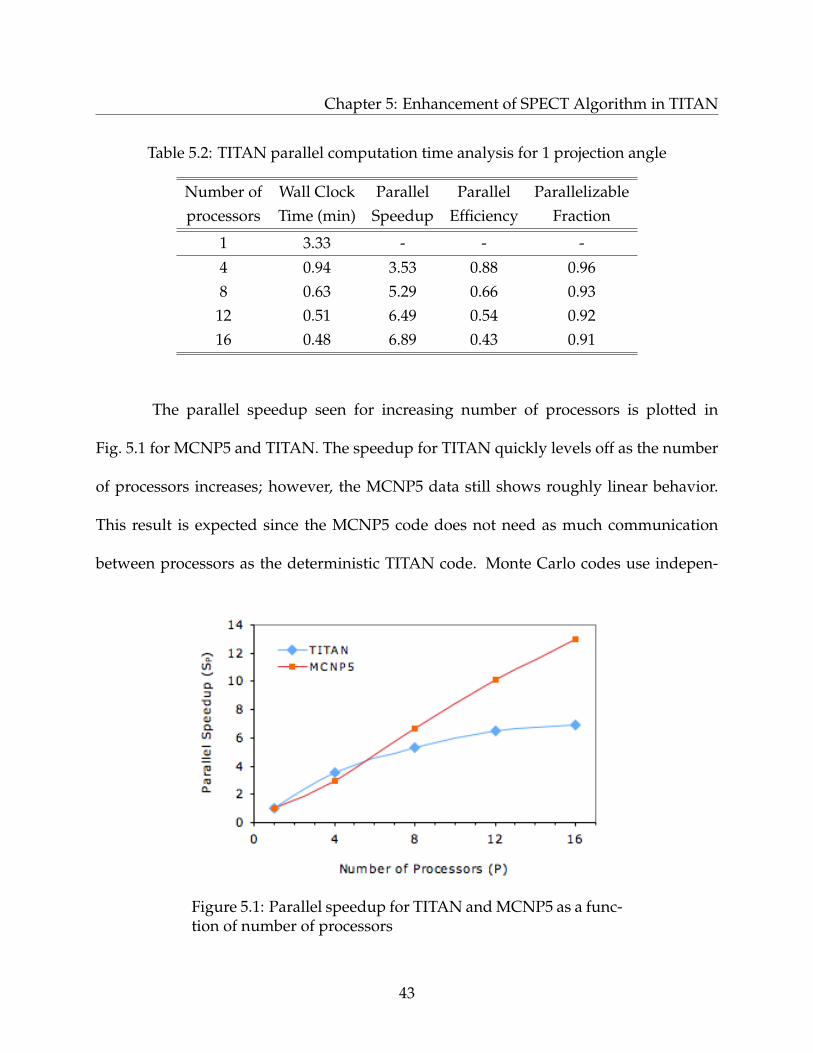
Chapter 5: Enhancement of SPECT Algorithm in TITAN
Table 5.2: TITAN parallel computation time analysis for 1 projection angle
Number of Wall Clock Parallel Parallel Parallelizableprocessors Time (min) Speedup Efficiency Fraction
1 3.33 - - -
4 0.94 3.53 0.88 0.968 0.63 5.29 0.66 0.93
12 0.51 6.49 0.54 0.9216 0.48 6.89 0.43 0.91
The parallel speedup seen for increasing number of processors is plotted in
Fig. 5.1 for MCNP5 and TITAN. The speedup for TITAN quickly levels off as the number
of processors increases; however, the MCNP5 data still shows roughly linear behavior.
This result is expected since the MCNP5 code does not need as much communication
between processors as the deterministic TITAN code. Monte Carlo codes use indepen-
Figure 5.1: Parallel speedup for TITAN and MCNP5 as a func-tion of number of processors
43
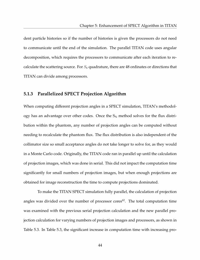
Chapter 5: Enhancement of SPECT Algorithm in TITAN
dent particle histories so if the number of histories is given the processors do not need
to communicate until the end of the simulation. The parallel TITAN code uses angular
decomposition, which requires the processors to communicate after each iteration to re-
calculate the scattering source. For S6 quadrature, there are 48 ordinates or directions that
TITAN can divide among processors.
5.1.3 Parallelized SPECT Projection Algorithm
When computing different projection angles in a SPECT simulation, TITAN’s methodol-
ogy has an advantage over other codes. Once the SN method solves for the flux distri-
bution within the phantom, any number of projection angles can be computed without
needing to recalculate the phantom flux. The flux distribution is also independent of the
collimator size so small acceptance angles do not take longer to solve for, as they would
in a Monte Carlo code. Originally, the TITAN code ran in parallel up until the calculation
of projection images, which was done in serial. This did not impact the computation time
significantly for small numbers of projection images, but when enough projections are
obtained for image reconstruction the time to compute projections dominated.
To make the TITAN SPECT simulation fully parallel, the calculation of projection
angles was divided over the number of processor cores62. The total computation time
was examined with the previous serial projection calculation and the new parallel pro-
jection calculation for varying numbers of projection images and processors, as shown in
Table 5.3. In Table 5.3, the significant increase in computation time with increasing pro-
44
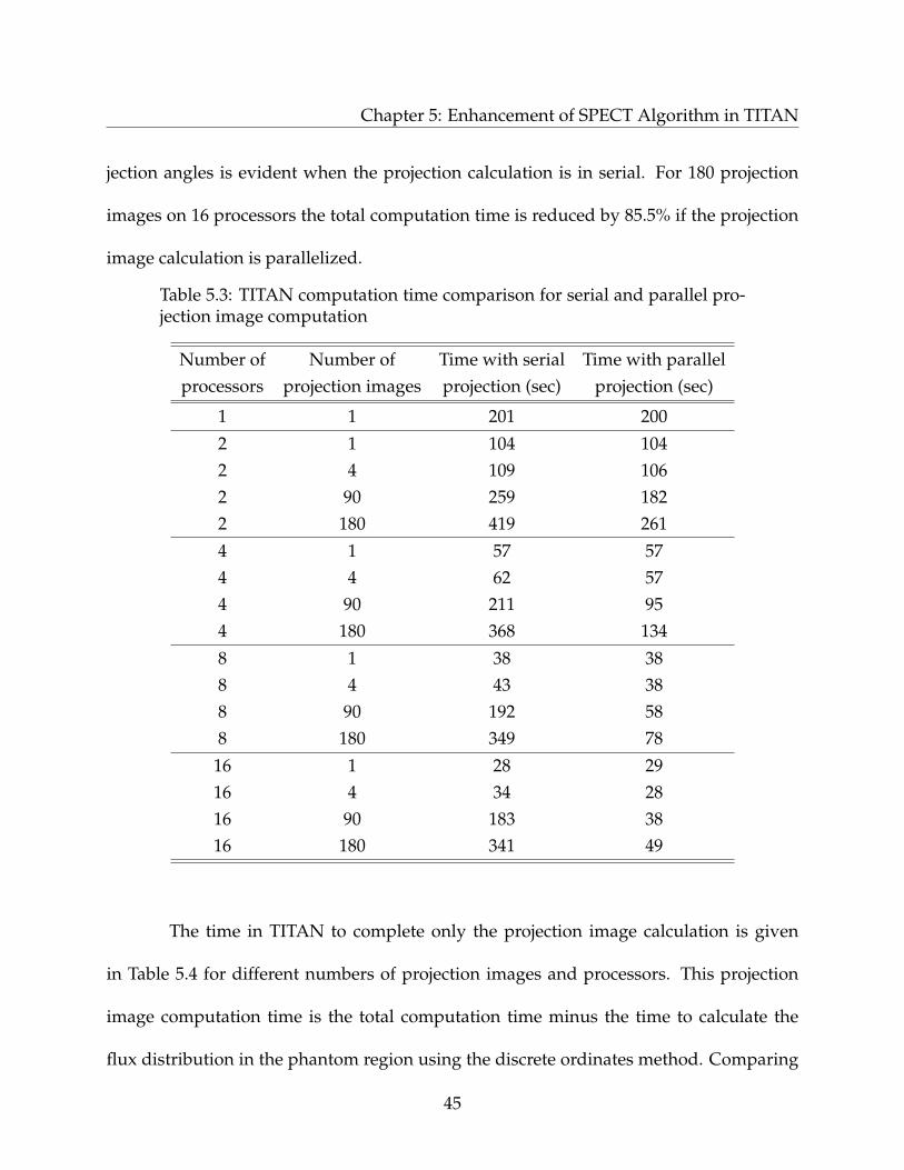
Chapter 5: Enhancement of SPECT Algorithm in TITAN
jection angles is evident when the projection calculation is in serial. For 180 projection
images on 16 processors the total computation time is reduced by 85.5% if the projection
image calculation is parallelized.
Table 5.3: TITAN computation time comparison for serial and parallel pro-jection image computation
Number of Number of Time with serial Time with parallelprocessors projection images projection (sec) projection (sec)
1 1 201 200
2 1 104 1042 4 109 1062 90 259 1822 180 419 261
4 1 57 574 4 62 574 90 211 954 180 368 134
8 1 38 388 4 43 388 90 192 588 180 349 78
16 1 28 2916 4 34 2816 90 183 3816 180 341 49
The time in TITAN to complete only the projection image calculation is given
in Table 5.4 for different numbers of projection images and processors. This projection
image computation time is the total computation time minus the time to calculate the
flux distribution in the phantom region using the discrete ordinates method. Comparing
45

Chapter 5: Enhancement of SPECT Algorithm in TITAN
the serial and parallel projection calculations, as expected, the times scale very closely
with the number of processors for the 2- and 4-processor cases. However, as was seen in
Table 5.3, there is some loss of speedup due to increased communication in the cases with
8 and 16 processors.
Table 5.4: TITAN projection image computation time comparison for serial and par-allel calculations
Number of Number of Serial projection image Parallel projection imageprocessors projection images calculation time (sec) calculation time (sec)
1 1 2.2 2.3
2 1 2.2 2.32 4 7.5 4.12 90 156.6 80.12 180 316.8 158.4
4 1 2.2 2.34 4 7.4 2.44 90 156.9 41.14 180 314.0 79.9
8 1 2.3 2.58 4 7.5 2.58 90 156.9 22.48 180 313.6 42.4
16 1 2.3 2.416 4 7.5 2.516 90 156.5 11.716 180 315.8 22.7
46

Chapter 5: Enhancement of SPECT Algorithm in TITAN
5.2 Weighted Circular Ordinate Splitting
As discussed in Section 4.2, the accuracy of the TITAN code’s COS technique for sim-
ulating the collimator with different acceptance angles62 has been examined. The work
found the TITAN methodology to be accurate for small acceptance angles, but with de-
creasing accuracy apparent for larger angles. While much larger acceptance angles may
not be practical for SPECT collimators, it is desired that the TITAN methodology be appli-
cable to a wide range of geometries and, therefore, applications. For example, modeling
streaming through ducts66 in a nuclear reactor to estimate dose to workers. In addition, it
would be desirable to further improve the accuracy for small acceptance angles and make
the collimator representation more physical.
A new methodology based on the COS technique for collimator representation
has been developed and implemented in the TITAN code: weighted circular ordinate
splitting67, 68 (WCOS). The original COS technique used a simple average of the angular
flux of all split directions and allowed the user to specify a single value for the number
of directions per concentric circle, referred to as the splitting order. The WCOS tech-
nique makes use of Riauka and Gortel’s (1994) collimator representation, which is part of
their analytical method to simulate SPECT34. In the new technique, the split directions
specified within a collimator acceptance angle are used to calculate a geometry-based
weighted average as shown in Figure 5.2. The weighting is determined by the overlap of
the detector surface area projection along the direction to the front of collimator. The split
47
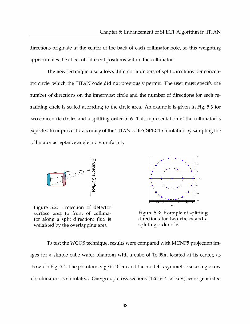
Chapter 5: Enhancement of SPECT Algorithm in TITAN
directions originate at the center of the back of each collimator hole, so this weighting
approximates the effect of different positions within the collimator.
The new technique also allows different numbers of split directions per concen-
tric circle, which the TITAN code did not previously permit. The user must specify the
number of directions on the innermost circle and the number of directions for each re-
maining circle is scaled according to the circle area. An example is given in Fig. 5.3 for
two concentric circles and a splitting order of 6. This representation of the collimator is
expected to improve the accuracy of the TITAN code’s SPECT simulation by sampling the
collimator acceptance angle more uniformly.
Figure 5.2: Projection of detectorsurface area to front of collima-tor along a split direction; flux isweighted by the overlapping area
Figure 5.3: Example of splittingdirections for two circles and asplitting order of 6
To test the WCOS technique, results were compared with MCNP5 projection im-
ages for a simple cube water phantom with a cube of Tc-99m located at its center, as
shown in Fig. 5.4. The phantom edge is 10 cm and the model is symmetric so a single row
of collimators is simulated. One-group cross sections (126.5-154.6 keV) were generated
48
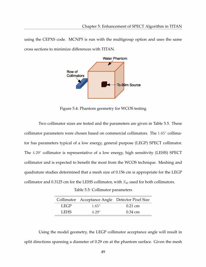
Chapter 5: Enhancement of SPECT Algorithm in TITAN
using the CEPXS code. MCNP5 is run with the multigroup option and uses the same
cross sections to minimize differences with TITAN.
Figure 5.4: Phantom geometry for WCOS testing
Two collimator sizes are tested and the parameters are given in Table 5.5. These
collimator parameters were chosen based on commercial collimators. The 1.65 collima-
tor has parameters typical of a low energy, general purpose (LEGP) SPECT collimator.
The 4.29 collimator is representative of a low energy, high sensitivity (LEHS) SPECT
collimator and is expected to benefit the most from the WCOS technique. Meshing and
quadrature studies determined that a mesh size of 0.156 cm is appropriate for the LEGP
collimator and 0.3125 cm for the LEHS collimator, with S20 used for both collimators.
Table 5.5: Collimator parameters
Collimator Acceptance Angle Detector Pixel Size
LEGP 1.65 0.21 cmLEHS 4.29 0.34 cm
Using the model geometry, the LEGP collimator acceptance angle will result in
split directions spanning a diameter of 0.29 cm at the phantom surface. Given the mesh
49

Chapter 5: Enhancement of SPECT Algorithm in TITAN
size for this phantom, it is determined that 2 splitting circles are needed to ensure that
enough voxels at the phantom surface are included to properly represent the collimator.
The normalized flux distribution at the detector as calculated by the TITAN code is com-
pared against MCNP5 results for the LEGP collimator in Fig. 5.5. MCNP5 1σ statistical
uncertainties are 0.8− 3.6% for this data. For normalized fluxes greater than 0.1, the aver-
age difference between the TITAN and MCNP5 results is 2.3%. For this small collimator
acceptance angle, no significant difference was observed between the original COS tech-
nique in TITAN and the new WCOS technique. As a further comparison, the full width
at half maximum (FWHM) is compared between the codes. In MCNP5 the FWHM is
1.27 cm and in TITAN it is 1.25 cm, for a relative difference of -1.2%.
Figure 5.5: TITAN and MCNP5(1σ 0.8 − 3.6%) flux distributions forLEGP collimator (1.65)
Figure 5.6: TITAN and MCNP5(1σ 0.4 − 4.4%) flux distributions forLEHS collimator (4.29)
Considering the LEHS collimator, projecting the collimator acceptance angle to
the phantom surface, split directions will span 0.75 cm. Considering the phantom mesh
size, it is determined that 2 splitting circles should be used for the LEHS case to include
enough voxels at the phantom surface. The normalized flux distributions with the LEHS
50
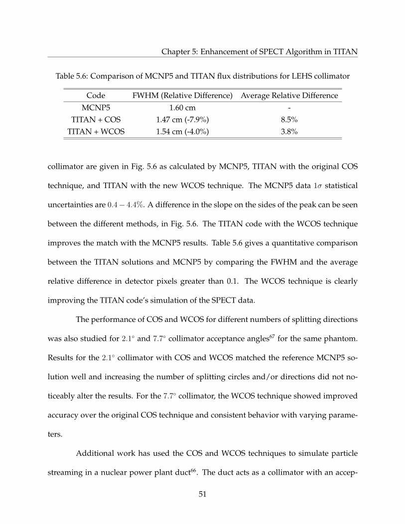
Chapter 5: Enhancement of SPECT Algorithm in TITAN
Table 5.6: Comparison of MCNP5 and TITAN flux distributions for LEHS collimator
Code FWHM (Relative Difference) Average Relative Difference
MCNP5 1.60 cm -TITAN + COS 1.47 cm (-7.9%) 8.5%
TITAN + WCOS 1.54 cm (-4.0%) 3.8%
collimator are given in Fig. 5.6 as calculated by MCNP5, TITAN with the original COS
technique, and TITAN with the new WCOS technique. The MCNP5 data 1σ statistical
uncertainties are 0.4− 4.4%. A difference in the slope on the sides of the peak can be seen
between the different methods, in Fig. 5.6. The TITAN code with the WCOS technique
improves the match with the MCNP5 results. Table 5.6 gives a quantitative comparison
between the TITAN solutions and MCNP5 by comparing the FWHM and the average
relative difference in detector pixels greater than 0.1. The WCOS technique is clearly
improving the TITAN code’s simulation of the SPECT data.
The performance of COS and WCOS for different numbers of splitting directions
was also studied for 2.1 and 7.7 collimator acceptance angles67 for the same phantom.
Results for the 2.1 collimator with COS and WCOS matched the reference MCNP5 so-
lution well and increasing the number of splitting circles and/or directions did not no-
ticeably alter the results. For the 7.7 collimator, the WCOS technique showed improved
accuracy over the original COS technique and consistent behavior with varying parame-
ters.
Additional work has used the COS and WCOS techniques to simulate particle
streaming in a nuclear power plant duct66. The duct acts as a collimator with an accep-
51

Chapter 5: Enhancement of SPECT Algorithm in TITAN
tance angle of 3.0. Compared with an MCNP5 reference solution, TITAN with COS and
TITAN with WCOS gave similar results, but the WCOS technique behaved more consis-
tently with increasing number of split directions.
52
Chapter 6
Implementation of the Novel Image
Reconstruction Methodology
In this chapter, a novel image reconstruction methodology that utilizes a deterministic
transport code is developed. Next, a framework for implementing the methodology with
any deterministic transport code is given in the form of a script. Finally, the methodology
is applied to a 2-dimensional reconstruction as a feasibility study.
6.1 DRS Methodology
When seeking to model particle transport in SPECT reconstruction, Monte Carlo methods
are the standard. Monte Carlo methods have the advantages of modeling exact geometry
and continuous energy, but tend to require long computation times to achieve accept-
able statistical uncertainties and provide limited information. In contrast, deterministic
53
Chapter 6: Novel Image Reconstruction Methodology
methods solve the linear Boltzmann equation numerically. They generally have shorter
computation times and provide large amounts of information, but the phase space is dis-
cretized and they can be memory intensive for achieving accurate results. With modern
computers, this memory requirement is less of a difficulty, and so deterministic methods
have the potential to provide an alternative to Monte Carlo methods.
This new deterministic reconstruction methodology for SPECT (DRS) was devel-
oped to take advantage of the TITAN deterministic transport code’s fast algorithm for
simulating SPECT projection images, but it could easily be used with other deterministic
codes. As discussed previously, the ML-EM reconstruction algorithm is the most common
for SPECT and will be used for this work; however, other iterative reconstruction algo-
rithms should be possible to apply. Recall that the ML-EM algorithm23 can be represented
by
λ(i+1)b = λ
(i)b
D∑d=1
n∗d
n(i)d
pb,d, b = 1, . . . , B, (6.1)
where λ(i)b is the ith estimate of the unknown source density in voxel b, n∗d is the measured
data in detector pixel d, n(i)d is the projection data using the last source estimate, and pb,d
(the system matrix) is the probability that a source particle emitted in voxel b is detected in
detector pixel d. The denominator in Eq. 6.1 is the ”forward” projection that is completed
by a deterministic transport code and the summation is the backprojection.
The steps for the DRS methodology are outlined in a flowchart given in Fig. 6.1.
In addition to the initial guess of the source distribution, the reference measured projec-
tion data and system matrix must be provided. Particle transport is then completed in the
54
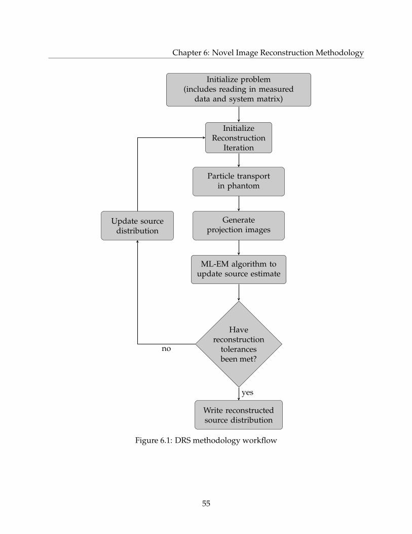
Chapter 6: Novel Image Reconstruction Methodology
Initialize problem(includes reading in measured
data and system matrix)
InitializeReconstruction
Iteration
Particle transportin phantom
Generateprojection images
Update sourcedistribution
ML-EM algorithm toupdate source estimate
Havereconstruction
tolerancesbeen met?
Write reconstructedsource distribution
no
yes
Figure 6.1: DRS methodology workflow
55

Chapter 6: Novel Image Reconstruction Methodology
phantom and the projection images based on the current estimate of the source distribu-
tion are created. These projections are passed to the ML-EM algorithm, which compares
them with the measured data and backprojects to update the source estimate. If tolerances
have not been met, the processes is restarted with the updated source distribution.
6.2 Analysis of DRS methodology
6.2.1 Framework Implementation
A framework was created based on the DRS methodology in the form of an image re-
construction script. The script iteratively calls the TITAN code and feeds the output into
an ML-EM algorithm. The script could be used to call any particle transport code that
generates projections at a detector for a given source distribution. With this implemen-
tation, the TITAN transport calculation can be run in parallel, but all other calculations
are in serial, including the ML-EM algorithm. Additional read/write times are associ-
ated with having an external script call TITAN iteratively; however, this script allows
for preliminary testing and troubleshooting of issues that appear before implementing
the reconstruction algorithm into the TITAN source code. This framework can be used
to demonstrate reasonable reconstruction computation times while allowing the perfor-
mance of a deterministic transport code as a forward projector to be analyzed.
Iterative reconstruction is implemented using a script with the following steps:
i. Initialize TITAN input file with a guess of the source distribution λ(0)
56
Chapter 6: Novel Image Reconstruction Methodology
ii. Call the TITAN SPECT simulation to obtain projection data n(i)
iii. Call the ML-EM algorithm to compare the generated projection data n(i) with the
measured data n∗ and generate the new updated source distribution λ(i+1)
iv. Update the estimated source distribution λ(i+1) in the TITAN input file.
Steps ii-iv are repeated until the maximum number of iterations has been completed or
some tolerance has been met. This procedure allows all interactions in the phantom to be
simulated in the forward projection step by TITAN. The ML-EM algorithm called in Step
iii is written in Fortran 95 and calculates the new source estimate using Eq. 6.1. The script
and the ML-EM code that it calls are given in Appendix A.
6.2.2 Phantom Studies
A simple 2-dimensional elliptical water phantom is reconstructed with the DRS script as
a feasibility study of the methodology. The water phantom has a background relative
source strength of 1 and two circles with source strengths of 2 to represent lesions, as
depicted in Fig. 6.2. The voxelized model has 64 by 64 voxels and is 22.4 cm by 22.4 cm.
It is important to note that the TITAN code is a 3-dimensional code that is being used to
complete a 2-dimensional reconstruction. This leads to some inefficiencies; in particular,
a 3-dimensional cylinder with no variation along z is modeled in TITAN to simulate this
2-dimensional phantom, as shown in Fig. 6.3.
57

Chapter 6: Novel Image Reconstruction Methodology
Figure 6.2: Reference source dis-tribution with source strengths of2 in white and 1 in gray Figure 6.3: TITAN 3-dimensional model
A flat source distribution of one is used for the initial guess λ(0). The system
matrix, pb,d, is obtained using Professor Jeff Fessler’s Image Reconstruction Toolbox36 for
MATLAB and models attenuation only, i.e., not scatter. The SIMIND Monte Carlo code31
is used to generate the measured projection data, which is displayed as a sinogram in
Fig. 6.4. Recall from Section 2.2 that in a sinogram the detector elements are displayed
along the horizontal axis and the projection angles are given along the vertical axis. In
Fig. 6.4, 120 projection images are obtained over 360 counter-clockwise around the phan-
tom with the initial angle located directly above the phantom in Fig. 6.2. Reconstructions
with 60 projection images obtained over 180 counter-clockwise around the left-hand side
of the phantom are also considered. The 60 projection reconstructions use the top half of
Fig. 6.4 as the measured projection data. The SIMIND data is for a long simulation, such
that the statistical uncertainty can be approximated as zero, and a perfect collimator, i.e.,
extremely narrow and no septal penetration, is simulated at this time.
58
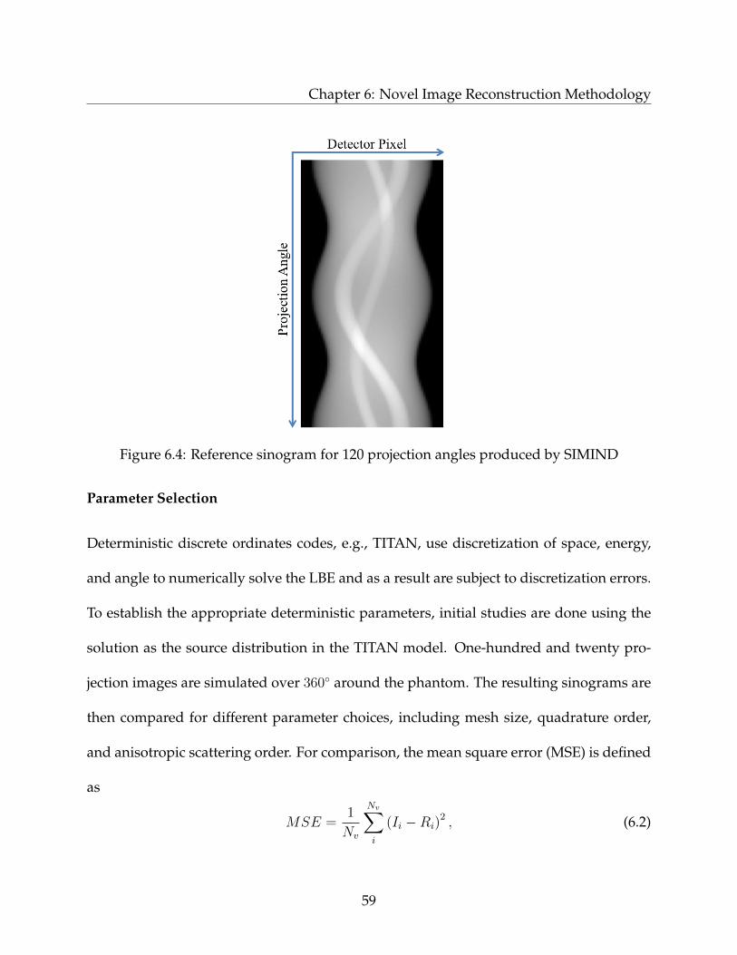
Chapter 6: Novel Image Reconstruction Methodology
Figure 6.4: Reference sinogram for 120 projection angles produced by SIMIND
Parameter Selection
Deterministic discrete ordinates codes, e.g., TITAN, use discretization of space, energy,
and angle to numerically solve the LBE and as a result are subject to discretization errors.
To establish the appropriate deterministic parameters, initial studies are done using the
solution as the source distribution in the TITAN model. One-hundred and twenty pro-
jection images are simulated over 360 around the phantom. The resulting sinograms are
then compared for different parameter choices, including mesh size, quadrature order,
and anisotropic scattering order. For comparison, the mean square error (MSE) is defined
as
MSE =1
Nv
Nv∑i
(Ii −Ri)2 , (6.2)
59

Chapter 6: Novel Image Reconstruction Methodology
where I is the simulation result for a particular set parameters,R is the reference solution,
and Nv is the number of detector pixels. The maximum relative difference is defined as
Max. rel. diff. = max
(Ii −Ri
Ri
)for i = 1 . . . Nv. (6.3)
To examine the sensitivity of results to mesh size, the number of meshes is dou-
bled in each dimension from each case number to the next, as shown in Table 6.1. The
mesh parameter h is defined as the mesh size relative to Case 3 (the finest mesh size).
Table 6.1: Meshing parameters
Case h Mesh size Number of meshes
1 4 3.50 mm 64 x 642 2 1.75 mm 128 x 1283 1 0.875 mm 256 x 256
The detector flux at different projection angles was plotted to ensure that the
mesh refinement was adequate. Selected plots are given in Fig. 6.5 for projection im-
ages at 21 and 141. The match with the reference SIMIND solution is seen to improve as
h decreases, i.e., decreasing mesh size, in the TITAN simulation. The h = 4 mesh shows a
few unphysical oscillations; however, the improvement from h = 2 to h = 1 is minimal.
The quadrature order was also examined from S12 to S40. The maximum rela-
tive difference and MSE of the TITAN sinogram relative to the S40 solution for different
quadrature orders is given in Table 6.2. A large reduction in differences is seen when the
quadrature is increased from S16 to S20.
60
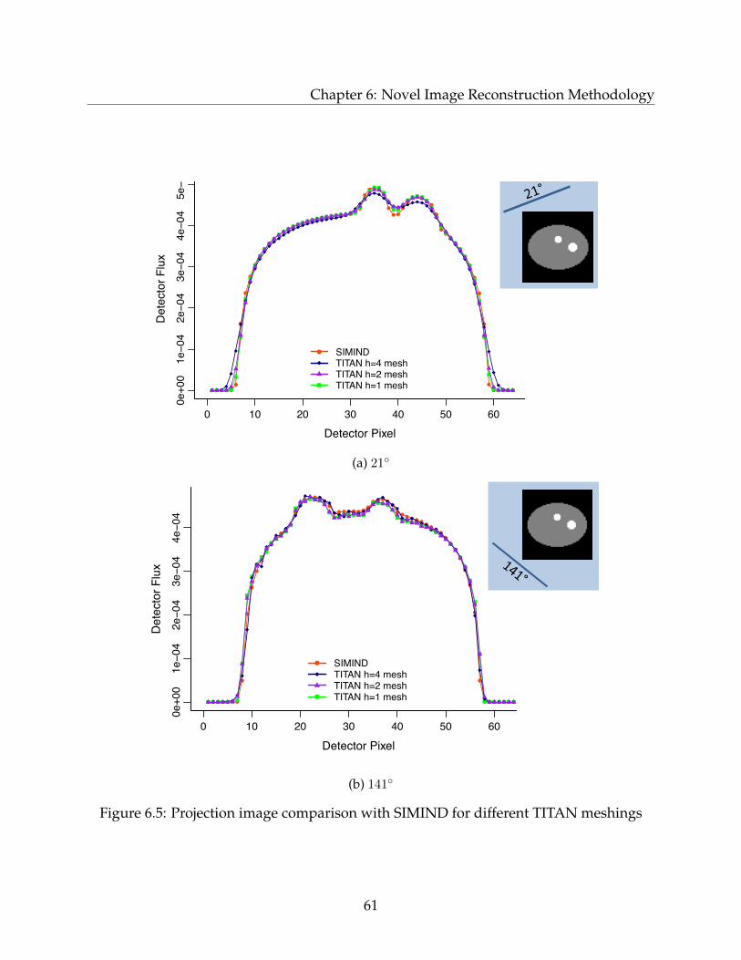
Chapter 6: Novel Image Reconstruction Methodology
0 10 20 30 40 50 60
0e+0
01e−0
42e−0
43e−0
44e−0
4
Detector Pixel
Det
ecto
r Flu
x
DTW S40 Projection 48
SIMINDTITAN h=4 meshTITAN h=2 meshTITAN h=1 mesh
0 10 20 30 40 50 60
0e+0
01e−0
42e−0
43e−0
44e−0
45e−0
4
Detector Pixel
Det
ecto
r Flu
xDTW S40 Projection 8
SIMINDTITAN h=4 meshTITAN h=2 meshTITAN h=1 mesh
(a) 21
0 10 20 30 40 50 60
0e+0
01e−0
42e−0
43e−0
44e−0
4
Detector Pixel
Det
ecto
r Flu
x
DTW S40 Projection 48
SIMINDTITAN h=4 meshTITAN h=2 meshTITAN h=1 mesh
0 10 20 30 40 50 60
0e+0
01e−0
42e−0
43e−0
44e−0
45e−0
4
Detector Pixel
Det
ecto
r Flu
xDTW S40 Projection 8
SIMINDTITAN h=4 meshTITAN h=2 meshTITAN h=1 mesh
(b) 141
Figure 6.5: Projection image comparison with SIMIND for different TITAN meshings
61
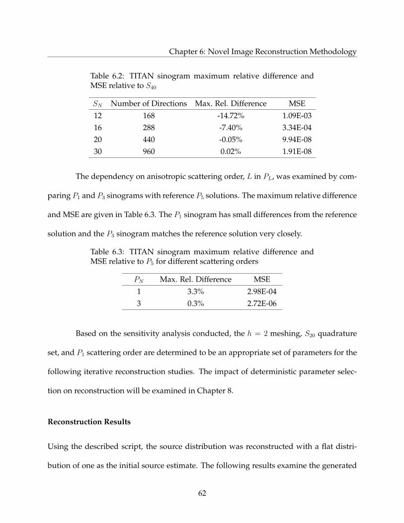
Chapter 6: Novel Image Reconstruction Methodology
Table 6.2: TITAN sinogram maximum relative difference andMSE relative to S40
SN Number of Directions Max. Rel. Difference MSE
12 168 -14.72% 1.09E-0316 288 -7.40% 3.34E-0420 440 -0.05% 9.94E-0830 960 0.02% 1.91E-08
The dependency on anisotropic scattering order, L in PL, was examined by com-
paring P1 and P3 sinograms with reference P5 solutions. The maximum relative difference
and MSE are given in Table 6.3. The P1 sinogram has small differences from the reference
solution and the P3 sinogram matches the reference solution very closely.
Table 6.3: TITAN sinogram maximum relative difference andMSE relative to P5 for different scattering orders
PN Max. Rel. Difference MSE
1 3.3% 2.98E-043 0.3% 2.72E-06
Based on the sensitivity analysis conducted, the h = 2 meshing, S20 quadrature
set, and P1 scattering order are determined to be an appropriate set of parameters for the
following iterative reconstruction studies. The impact of deterministic parameter selec-
tion on reconstruction will be examined in Chapter 8.
Reconstruction Results
Using the described script, the source distribution was reconstructed with a flat distri-
bution of one as the initial source estimate. The following results examine the generated
62

Chapter 6: Novel Image Reconstruction Methodology
sinograms and source distributions for measured data over 180 and 360, as well as the
convergence of the reconstruction.
Using measured projections over 180, the sinograms generated by TITAN and
the reconstructed source distributions after 5, 10, 20, and 40 iterations are given in Figs. 6.6
and 6.7, respectively. The TITAN forward projection uses the S20 quadrature set and
the DDZ (diamond differencing with zero fix-up) differencing scheme, as discussed in
Section 3.1. In Figs. 6.6a and 6.7a, the source distribution is already taking shape after
5 iterations; however, with additional iterations an artifact in the form of ripples near
the right edge of the phantom is present. This artifact grows with increasing numbers of
iterations and is attributed to the measured sinogram data being limited to the left-hand
side of the phantom. The DTW (directional theta weighted) differencing scheme56 should
be less susceptible to unphysical oscillations than the DDZ differencing scheme for the
same discretization. The sinograms generated by TITAN and the reconstructed source
distributions after 5, 10, 20, and 40 iterations are given in Figs. 6.8 and 6.9, respectively,
for S20 and the DTW differencing scheme. The ripple artifact is significantly reduced,
compared to the DDZ result, but some oscillations are still present on the right-hand side
of the reconstruction. A bright ring of source is also appearing around the phantom edge
with increasing iterations.
Reconstruction is now done using 120 projection angles over 360 around the
phantom to determine if the artifacts seen in Figs. 6.7 and 6.9 are due to a lack of infor-
mation about the right-hand side of the phantom. The reconstructed source distributions
63
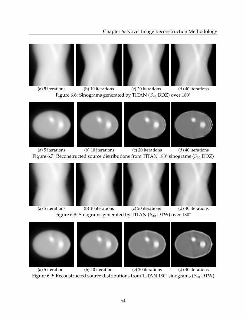
Chapter 6: Novel Image Reconstruction Methodology
(a) 5 iterations (b) 10 iterations (c) 20 iterations (d) 40 iterationsFigure 6.6: Sinograms generated by TITAN (S20 DDZ) over 180
(a) 5 iterations (b) 10 iterations (c) 20 iterations (d) 40 iterationsFigure 6.7: Reconstructed source distributions from TITAN 180 sinograms (S20 DDZ)
(a) 5 iterations (b) 10 iterations (c) 20 iterations (d) 40 iterationsFigure 6.8: Sinograms generated by TITAN (S20 DTW) over 180
(a) 5 iterations (b) 10 iterations (c) 20 iterations (d) 40 iterationsFigure 6.9: Reconstructed source distributions from TITAN 180 sinograms (S20 DTW)
64

Chapter 6: Novel Image Reconstruction Methodology
(a) 5 iterations (b) 10 iterations (c) 20 iterations (d) 40 iterationsFigure 6.10: Reconstructed source distributions from TITAN 360 sinograms (S20 DDZ)
(a) 5 iterations (b) 10 iterations (c) 20 iterations (d) 40 iterationsFigure 6.11: Reconstructed source distributions from TITAN 360 sinograms (S20 DTW)
for 5, 10, 20, and 40 iterations are given in Figs. 6.10 and 6.11 for DDZ and DTW, respec-
tively. Using measured projection data over 360 has removed the ripple artifact from the
reconstructed source and generally improved the reconstruction visually, but the bright
ring of source around the phantom edge persists above 20 iterations.
The edge, or ring, artifact was initially thought to be caused by the differenc-
ing scheme used by TITAN being inadequate at source discontinuities. Petrovic and
Haghighat53 showed that unphysical oscillations, that are not ray effects, can occur at
discontinuities due to the inconsistency between particle direction and the spatial dif-
ferencing axis. These oscillations can not be removed by mesh refinement. The DTW
differencing scheme69 was developed to minimize oscillations by incorporating particle
65

Chapter 6: Novel Image Reconstruction Methodology
0 5 10 20 30 40 50 60
0.0
0.4
0.8
1.2
1.6
2.0
Phantom Voxel
Sou
rce
Str
engt
h
Source Distribution
10 iterations20 iterations40 iterations
Figure 6.12: Horizontal profilethrough reconstructed source distri-bution with DDZ scheme
0 5 10 20 30 40 50 60
0.0
0.4
0.8
1.2
1.6
2.0
Phantom VoxelS
ourc
e S
tren
gth
Source Distribution
10 iterations20 iterations40 iterations
Figure 6.13: Horizontal profilethrough reconstructed source distri-bution with DTW scheme
direction into the differencing scheme. It may be that the oscillations at the edge of the
phantom are magnified over the iterations to create the ring artifact.
To further examine these results, horizontal profiles through the center of the
reconstructed source distributions are given in Figs. 6.12 and 6.13 for DDZ and DTW, re-
spectively, at 10, 20, and 40 iterations. Fig. 6.12 shows some oscillation at the phantom
edge and an excellent representation of the source distribution within the phantom, as
the number of iterations reaches 40 using DDZ. The reconstruction with DTW, Fig. 6.13,
overshoots the source at the edge of both the phantom and the circle of increased source
strength. This issue begins to appear for as few as 10 iterations and becomes larger with
additional iterations. The DDZ solution appears to be adequate for this model and will be
used in the following analysis, but in Section 8.1 the limitations of DDZ will be encoun-
tered and DTW will be used.
66

Chapter 6: Novel Image Reconstruction Methodology
(a) 5 iterations (b) 10 iterations (c) 20 iterations (d) 40 iterationsFigure 6.14: Reconstructed source distributions using the system matrix only
A literature search revealed that edge artifacts that resemble the Gibb’s phe-
nomenon are inherent to the ML-EM algorithm where source discontinuities occur70. Sny-
der et al. concluded that these artifacts can be caused by the numerical precision of the
computer, small mismatches between model and simulation, and other effects. To test this
possible origin of the ring artifact, an ML-EM reconstruction was done using the system
matrix only, i.e., without TITAN. The reconstructed source distributions for 5, 10, 20, and
40 iterations are given in Fig. 6.14 and closely resemble those produced using TITAN. The
ring artifact begins to appear in iteration 20 and becomes brighter by 40 iterations.
Horizontal and vertical profiles through the center of the reconstruction after 40
iterations are shown in Figs. 6.15 and 6.16, respectively, for reconstruction with TITAN
and with the system matrix (SM) only. In the phantom interior, the TITAN reconstruction
better represents the true source distribution. At the edge of the phantom, while both re-
constructions show oscillations, the oscillations do appear to be larger in these particular
profiles for the reconstruction with TITAN. This leads to the conclusion that the edge ar-
tifact may be contributed to by both the differencing scheme and the oscillations inherent
to ML-EM.
67
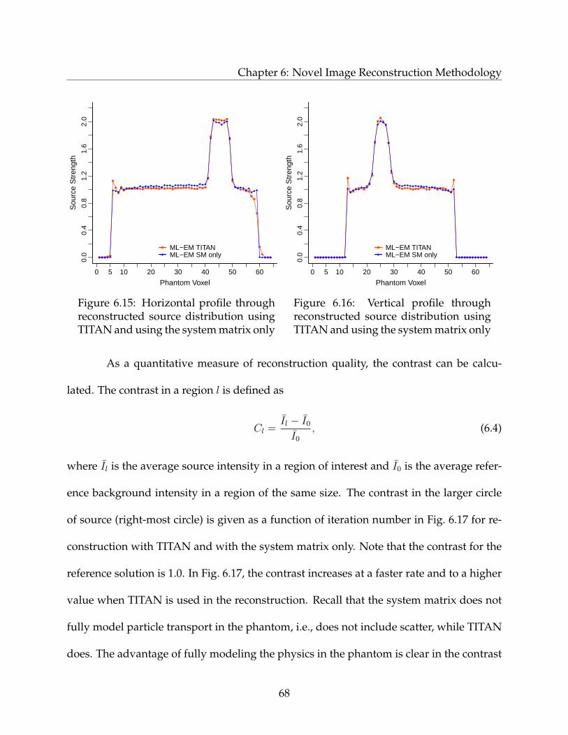
Chapter 6: Novel Image Reconstruction Methodology
0 5 10 20 30 40 50 60
0.0
0.4
0.8
1.2
1.6
2.0
Phantom Voxel
Sou
rce
Str
engt
h
Source Distribution
ML−EM TITANML−EM SM only
Figure 6.15: Horizontal profile throughreconstructed source distribution usingTITAN and using the system matrix only
0 5 10 20 30 40 50 60
0.0
0.4
0.8
1.2
1.6
2.0
Phantom VoxelS
ourc
e S
tren
gth
Source Distribution
ML−EM TITANML−EM SM only
Figure 6.16: Vertical profile throughreconstructed source distribution usingTITAN and using the system matrix only
As a quantitative measure of reconstruction quality, the contrast can be calcu-
lated. The contrast in a region l is defined as
Cl =Il − I0
I0
, (6.4)
where Il is the average source intensity in a region of interest and I0 is the average refer-
ence background intensity in a region of the same size. The contrast in the larger circle
of source (right-most circle) is given as a function of iteration number in Fig. 6.17 for re-
construction with TITAN and with the system matrix only. Note that the contrast for the
reference solution is 1.0. In Fig. 6.17, the contrast increases at a faster rate and to a higher
value when TITAN is used in the reconstruction. Recall that the system matrix does not
fully model particle transport in the phantom, i.e., does not include scatter, while TITAN
does. The advantage of fully modeling the physics in the phantom is clear in the contrast
68
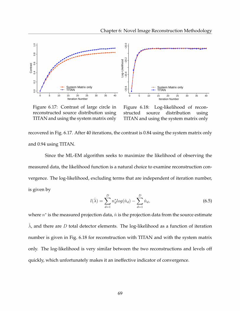
Chapter 6: Novel Image Reconstruction Methodology
0 5 10 15 20 25 30 35 40
0.0
0.2
0.4
0.6
0.8
1.0
Iteration Number
Con
tras
t
Contrast
System Matrix onlyTITAN
Figure 6.17: Contrast of large circle inreconstructed source distribution usingTITAN and using the system matrix only
0 5 10 15 20 25 30 35 40
−20
.6−
20.4
−20
.2−
20.0
Iteration Number
Log−
Like
lihoo
d
Contrast
System Matrix onlyTITAN
Figure 6.18: Log-likelihood of recon-structed source distribution usingTITAN and using the system matrix only
recovered in Fig. 6.17. After 40 iterations, the contrast is 0.84 using the system matrix only
and 0.94 using TITAN.
Since the ML-EM algorithm seeks to maximize the likelihood of observing the
measured data, the likelihood function is a natural choice to examine reconstruction con-
vergence. The log-likelihood, excluding terms that are independent of iteration number,
is given by
l(λ) =D∑d=1
n∗dlog(nd)−D∑d=1
nd, (6.5)
where n∗ is the measured projection data, n is the projection data from the source estimate
λ, and there are D total detector elements. The log-likelihood as a function of iteration
number is given in Fig. 6.18 for reconstruction with TITAN and with the system matrix
only. The log-likelihood is very similar between the two reconstructions and levels off
quickly, which unfortunately makes it an ineffective indicator of convergence.
69

Chapter 6: Novel Image Reconstruction Methodology
Computation Time
All calculations in this chapter were completed on a dedicated computer cluster with Intel
Xeon E5 2.6 GHz processors and 16 GB of memory per processor core. The reconstruction
script calls TITAN in parallel on 16 cores and the rest of the ML-EM reconstruction is done
in serial. Each forward projection of 120 projection images in TITAN took approximately
15 seconds. The computation time for reconstruction with 120 projection angles at differ-
ent numbers of iterations is given in Table 6.4 along with the corresponding contrast in
the large circle of source.
Table 6.4: Contrast and computation time of the re-constructed source distribution at different iterations
Iteration Contrast Computation Time
5 0.40 2.9 min10 0.63 6.3 min20 0.83 13.4 min40 0.94 27.4 min
Most of the computation time in Table 6.4 is spent reading and writing files, be-
cause the script externally calls TITAN for each iteration with the updated source distri-
bution. The computation time is expected to be significantly reduced by incorporating
the ML-EM algorithm directly into the TITAN source code. In addition to removing the
repeating reading and writing of files, this will also allow the ML-EM algorithm to be
parallelized.
70
Chapter 7
Development of TITAN-IR Algorithm
In this chapter, the steps involved in implementing the DRS methodology into the TITAN
source code are discussed, including the parallelization of the code. The modified version
of TITAN is called TITAN-IR (TITAN with image reconstruction).
7.1 TITAN-IR Algorithm
The image reconstruction process implemented in TITAN-IR is outlined in Fig. 7.1. For
the case of ML-EM reconstruction, there is one subset, i.e., Nsubsets = 1, which contains
all projection angles. The initial source estimate λ(0) is given in the input file and usually
specified as a uniform source. The measured projection data and system matrix must be
provided. A transport calculation is then completed based on the current source estimate
to find the converged flux moments for the phantom. Next, as described in Section 3.2.3,
the fictitious quadrature directions (µ(fix), ϕ(fic)) are generated for each projection angle
71
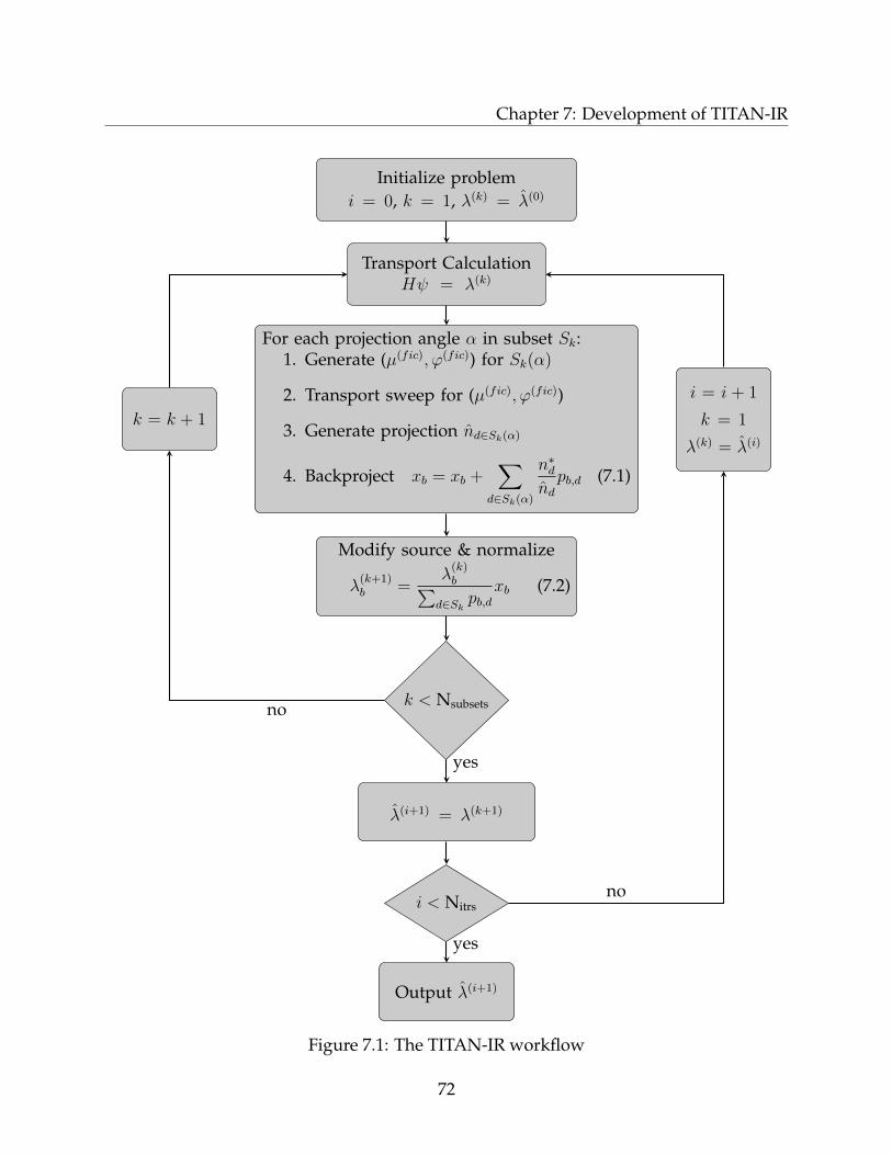
Chapter 7: Development of TITAN-IR
Initialize problemi = 0, k = 1, λ(k) = λ(0)
Transport CalculationHψ = λ(k)
For each projection angle α in subset Sk:1. Generate (µ(fic), ϕ(fic)) for Sk(α)
2. Transport sweep for (µ(fic), ϕ(fic))
3. Generate projection nd∈Sk(α)
4. Backproject xb = xb +∑
d∈Sk(α)
n∗dndpb,d (7.1)
Modify source & normalize
λ(k+1)b =
λ(k)b∑
d∈Skpb,d
xb (7.2)
k < Nsubsets
k = k + 1
λ(i+1) = λ(k+1)
i < Nitrs
Output λ(i+1)
i = i + 1
k = 1
λ(k) = λ(i)
no
yes
yes
no
Figure 7.1: The TITAN-IR workflow
72
Chapter 7: Development of TITAN-IR
α, a transport sweep is completed for each fictitious direction, and ray-tracing is used to
generate the projection images n. For each angle, the projection n is normalized to the
same total number of counts as the measured data. The resulting projection is then com-
pared with the measured data n∗ and backprojected using the system matrix p in Eq. 7.1.
These backprojections x are summed over all projection angles. Once all angles have
been iterated through, in Eq. 7.2 the backprojections are normalized and used to update
the source estimate. Other tolerances could be used, but generally ML-EM reconstruction
is terminated after a set number of iterations Nitrs have been completed.
7.2 TITAN-IR Implementation
Details on TITAN-IR input specifications are given in Appendix B. Deterministic codes
already tend to require large amounts of memory so the additional memory required for
the reconstruction should be considered. The primary additional memory requirement
is the system matrix which has dimensions of the number of phantom voxels by the to-
tal number of detector elements over all projection angles. The code in Appendix B.3
converts a system matrix into the appropriate sparse matrix format, but for some 3-D
simulations the system matrix size can still be on the order of gigabytes.
A low-pass filter has been implemented in the TITAN-IR algorithm to filter out
the high-frequency noise common to ML-EM reconstructed images. The Butterworth fil-
ter was chosen because it is a popular filter for SPECT, but additional filter options could
easily be added. The Butterworth filter is a low-pass filter, i.e., it does not alter low fre-
73
Chapter 7: Development of TITAN-IR
quencies and blocks high frequencies. The FFTW free-software library is used to compute
the discrete Fourier transform71 of the image. The Butterworth filter is given by
B(f) =1√
1 +(ffc
)2n, (7.3)
where f is the frequency, n is the order, and fc is the cutoff frequency. The cutoff frequency
defines the frequency at which the filter amplitude begins to drop and the order changes
the rate at which the filter amplitude goes to zero.
7.2.1 Parallel Implementation
In parallel transport calculations, the TITAN code divides the directions specified in the
quadrature set over the available processor cores in what is referred to as angular decom-
position. The parallel calculation is most efficient if the directions can be divided evenly
over the available processors, but this is not a requirement. After determining the particle
distribution in the phantom, each processor core calculates the projection images for its
assigned angles in parallel. The processors then communicate to merge the projection im-
ages calculated on each processor into one complete sinogram, which is written to a file.
Any time a parallel code must communicate amongst processors, the parallel efficiency is
reduced.
To take advantage of the parallelization of the projection image calculation, the
TITAN-IR backprojection step is also split across the processor cores and takes place after
each projection image is calculated, but before the cores communicate. For each angle,
74
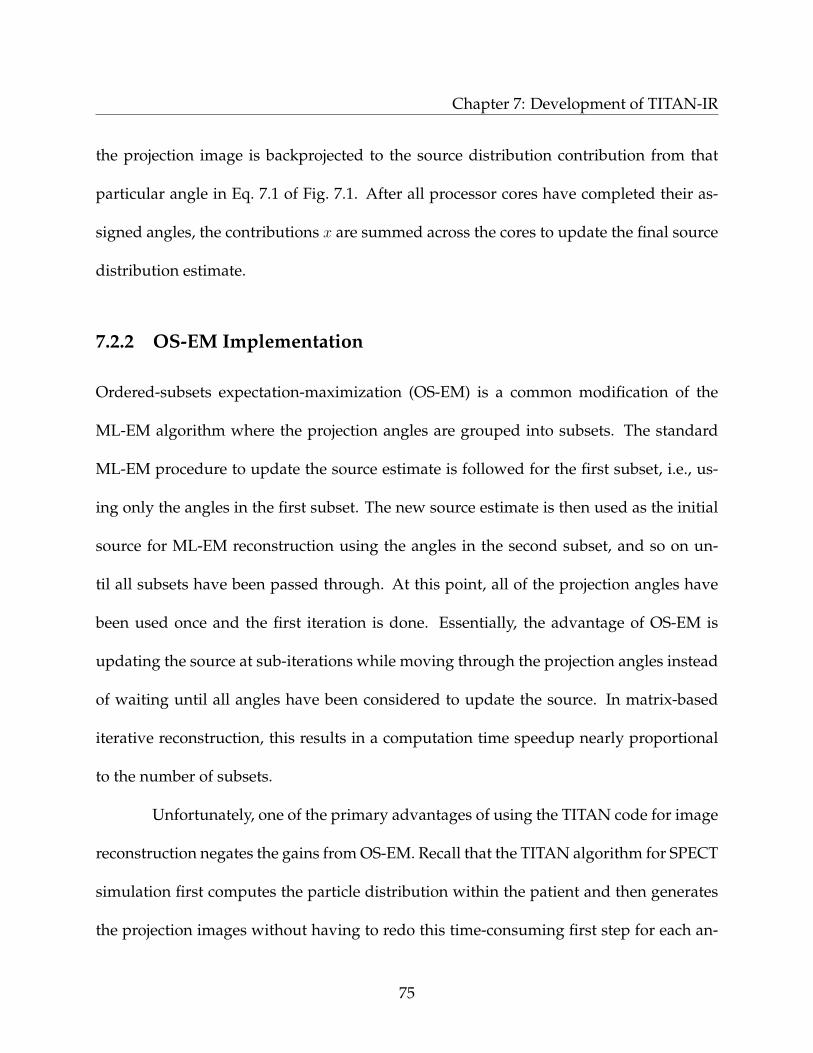
Chapter 7: Development of TITAN-IR
the projection image is backprojected to the source distribution contribution from that
particular angle in Eq. 7.1 of Fig. 7.1. After all processor cores have completed their as-
signed angles, the contributions x are summed across the cores to update the final source
distribution estimate.
7.2.2 OS-EM Implementation
Ordered-subsets expectation-maximization (OS-EM) is a common modification of the
ML-EM algorithm where the projection angles are grouped into subsets. The standard
ML-EM procedure to update the source estimate is followed for the first subset, i.e., us-
ing only the angles in the first subset. The new source estimate is then used as the initial
source for ML-EM reconstruction using the angles in the second subset, and so on un-
til all subsets have been passed through. At this point, all of the projection angles have
been used once and the first iteration is done. Essentially, the advantage of OS-EM is
updating the source at sub-iterations while moving through the projection angles instead
of waiting until all angles have been considered to update the source. In matrix-based
iterative reconstruction, this results in a computation time speedup nearly proportional
to the number of subsets.
Unfortunately, one of the primary advantages of using the TITAN code for image
reconstruction negates the gains from OS-EM. Recall that the TITAN algorithm for SPECT
simulation first computes the particle distribution within the patient and then generates
the projection images without having to redo this time-consuming first step for each an-
75
Chapter 7: Development of TITAN-IR
gle. This procedure allows TITAN to rapidly simulate a large number of projection angles,
but means that breaking the angles into subsets saves only a small amount of computa-
tion time. OS-EM was still implemented in TITAN-IR because of its wide-spread use and
because some modest reduction in computation time is expected.
To implement OS-EM in TITAN-IR, a loop was added within the outer reconstruc-
tion iteration loop to step through the subsets S1, S2, . . . , SNsubsetsas depicted in Fig. 7.1.
Each loop through a subset Sk is referred to as a sub-iteration k and a full iteration i is
only completed when all of the subsets have been iterated through. The angles can be
grouped into subsets in any number of ways, but dividing the angles equally into sub-
sets of opposing angles was recommended in the literature and, therefore, chosen for this
application. The TITAN-IR code groups the opposing angles into subsets and only uses
the angles assigned to the current subset for each sub-iteration. The source estimate λ(k)
is updated after each sub-iteration k. Note that the number of subsets must divide evenly
into the number of projection angles. A traditional ML-EM reconstruction can be done by
specifying 1 subset.
7.3 Quality Metrics
Several quality metrics are calculated for each iteration in TITAN-IR to assist in evaluating
how well the reconstruction algorithm is functioning. Image quality in nuclear medicine
is typically measured by spatial resolution, contrast and noise1. Spatial resolution in-
dicates the image sharpness or detail and is primarily limited by collimator resolution.
76
Chapter 7: Development of TITAN-IR
Collimator resolution can be improved with smaller collimator holes, but this is at the
expense of collimator efficiency and, therefore, increased noise. While it is important that
the model properly represents the collimator resolution, this is not a relevant metric for
evaluating the new image reconstruction algorithm; however, contrast and noise are im-
portant values to consider, in particular with relation to iteration number. The following
image quality metrics are calculated by TITAN-IR.
Differences in image intensity in adjacent regions of an image are referred to as
contrast3. In nuclear medicine, these differences in intensity correspond to levels of ra-
dioactive uptake in the patient and, therefore, number of disintegrations. The contrast in
a region l can be defined as
Cl =Il − I0
I0
(7.4)
where Il is the average image intensity in a region of interest, e.g., a lesion, and I0 is
the average reference background intensity, e.g., normal tissue. For contrast calculations,
TITAN-IR allows the user to specify multiple circular regions of interest and a reference
background region, as described further in Appendix B. The TITAN-IR code prints out
the contrast for each lesion for every iteration.
In ML-EM or OS-EM reconstruction, the increase of noise with number of itera-
tions is an important metric to consider. The noise is estimated for a background region
of the reconstructed image as a measure of this and is given by
noise =1
I0
√∑NV
i=1(Ii − I0)2
NV − 1(7.5)
77

Chapter 7: Development of TITAN-IR
where the Ii is the value in voxel i of the measured background region, I0 is the average
intensity, and NV is the number of voxels in the background region. This metric is output
for every iteration.
The above metrics are used to directly evaluate the reconstructed image. The
sinogram generated by the forward projection step was also evaluated by considering
the mean squared error (MSE) and mean relative error (MRE) relative to the measured
sinogram data. The MSE is given by
MSE =1
Nd
Nd∑d
(n
(i)d − n
∗d
)2
, (7.6)
where n(i)d is the counts in detector element d at iteration i, n∗d is the measured counts in
detector element d, and Nd is the total number of detector pixels. The MRE is given by
MRE =1
Nd
Nd∑d
∣∣∣∣∣ n(i)d − n∗dn∗d
∣∣∣∣∣ , (7.7)
where the variables are the same as in Eq. 7.6.
78

Chapter 8
Analysis of TITAN-IR
In this chapter, the TITAN-IR code is used to reconstruct the source distribution of two
phantoms: a quality assurance phantom and an anatomical torso phantom. The sensitiv-
ity of the reconstruction to deterministic parameters, noisy projection data, and collimator
blur is considered. Results will also be compared with FBP and ML-EM reconstruction
with the system matrix only.
8.1 Jaszczak Phantom with Cold Spheres
The Data Spectrum Corporation’s Jaszczak phantom is a popular phantom for quality
assurance in nuclear medicine. This cylindrical phantom consists of two regions: the
lower half with numerous rods of varying sizes and the upper half with six spheres of
different radii. The upper half of the phantom is modeled for this research with cold
79

Chapter 8: Analysis of TITAN-IR
spheres, i.e., spheres with no source, in a uniform background source of Tc-99m. A 3-
dimensional depiction of this geometry is given in Fig. 8.1. A slice through the center of
the source distribution is shown in Fig. 8.2.
Figure 8.1: Geometry of Jaszczak cylindrical phan-tom with cold spheres
Figure 8.2: Source distribu-tion in center slice of Jaszczakcylindrical phantom with coldspheres
The phantom cylinder has an outer diameter of 22.24 cm and is 11.12 cm tall. The
cylinder walls are 0.32 cm thick and made of PMMA (polymethyl methacrylate), as are
the cold spheres. The cold spheres have radii of 0.635, 0.795, 0.955, 1.27, 1.59, and 1.9 cm.
The phantom is then filled with water mixed with Tc-99m.
A flat source distribution of one is used for the initial guess of all reconstructions.
The system matrix is obtained using the Image Reconstruction Toolbox36 for MATLAB
and models attenuation and, where applicable, depth-dependent collimator blur. The
SIMIND Monte Carlo code is used to generate the ”measured” projection data for three
different conditions: i) noiseless projection data with no collimator blur, ii) noisy projec-
tion data with no collimator blur, and iii) noisy collimated projection data. Each projection
80
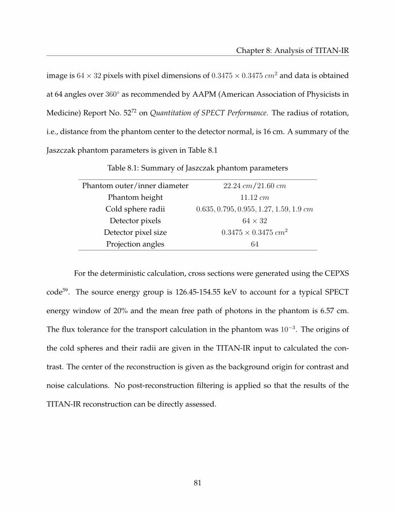
Chapter 8: Analysis of TITAN-IR
image is 64× 32 pixels with pixel dimensions of 0.3475× 0.3475 cm2 and data is obtained
at 64 angles over 360 as recommended by AAPM (American Association of Physicists in
Medicine) Report No. 5272 on Quantitation of SPECT Performance. The radius of rotation,
i.e., distance from the phantom center to the detector normal, is 16 cm. A summary of the
Jaszczak phantom parameters is given in Table 8.1
Table 8.1: Summary of Jaszczak phantom parameters
Phantom outer/inner diameter 22.24 cm/21.60 cm
Phantom height 11.12 cm
Cold sphere radii 0.635, 0.795, 0.955, 1.27, 1.59, 1.9 cm
Detector pixels 64× 32
Detector pixel size 0.3475× 0.3475 cm2
Projection angles 64
For the deterministic calculation, cross sections were generated using the CEPXS
code59. The source energy group is 126.45-154.55 keV to account for a typical SPECT
energy window of 20% and the mean free path of photons in the phantom is 6.57 cm.
The flux tolerance for the transport calculation in the phantom was 10−3. The origins of
the cold spheres and their radii are given in the TITAN-IR input to calculated the con-
trast. The center of the reconstruction is given as the background origin for contrast and
noise calculations. No post-reconstruction filtering is applied so that the results of the
TITAN-IR reconstruction can be directly assessed.
81
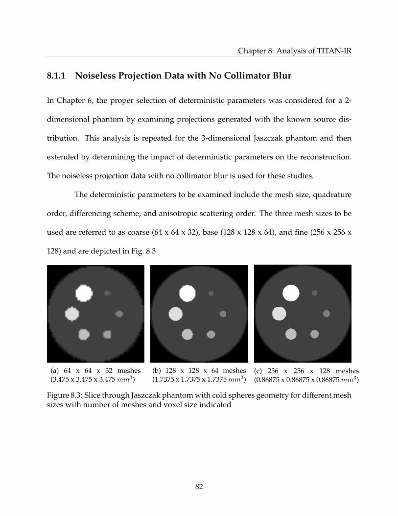
Chapter 8: Analysis of TITAN-IR
8.1.1 Noiseless Projection Data with No Collimator Blur
In Chapter 6, the proper selection of deterministic parameters was considered for a 2-
dimensional phantom by examining projections generated with the known source dis-
tribution. This analysis is repeated for the 3-dimensional Jaszczak phantom and then
extended by determining the impact of deterministic parameters on the reconstruction.
The noiseless projection data with no collimator blur is used for these studies.
The deterministic parameters to be examined include the mesh size, quadrature
order, differencing scheme, and anisotropic scattering order. The three mesh sizes to be
used are referred to as coarse (64 x 64 x 32), base (128 x 128 x 64), and fine (256 x 256 x
128) and are depicted in Fig. 8.3.
(a) 64 x 64 x 32 meshes(3.475 x 3.475 x 3.475 mm3)
(b) 128 x 128 x 64 meshes(1.7375 x 1.7375 x 1.7375mm3)
(c) 256 x 256 x 128 meshes(0.86875 x 0.86875 x 0.86875 mm3)
Figure 8.3: Slice through Jaszczak phantom with cold spheres geometry for different meshsizes with number of meshes and voxel size indicated
82
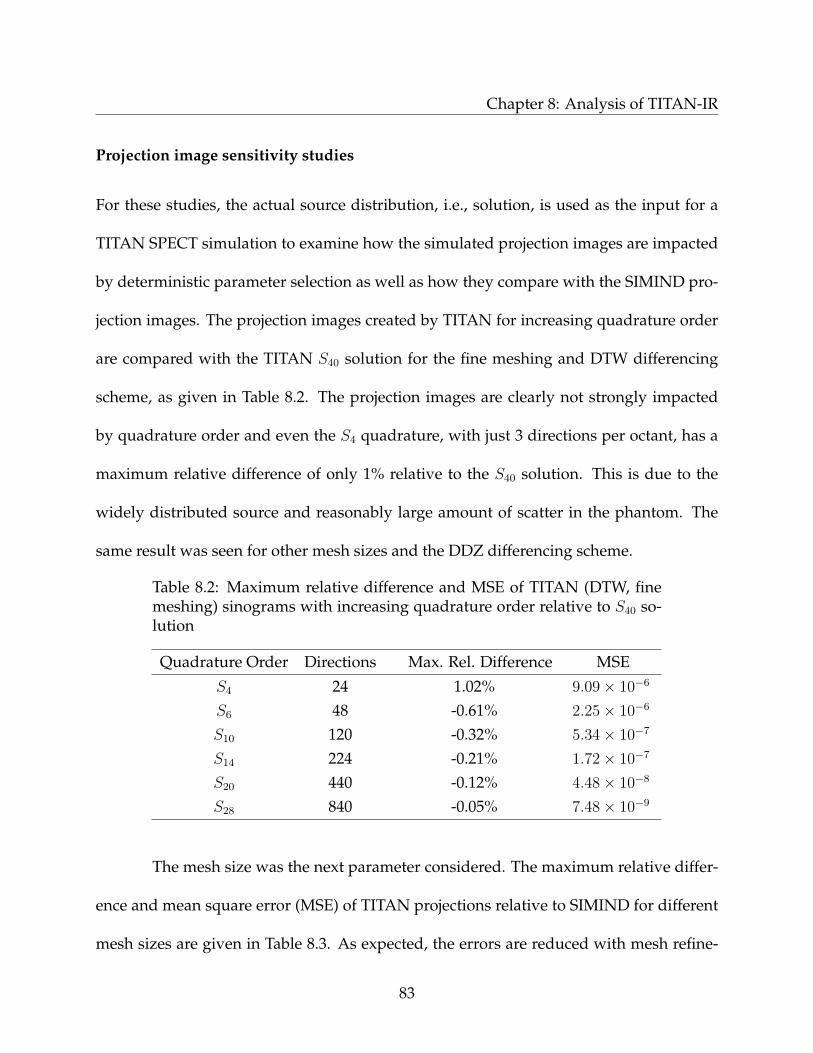
Chapter 8: Analysis of TITAN-IR
Projection image sensitivity studies
For these studies, the actual source distribution, i.e., solution, is used as the input for a
TITAN SPECT simulation to examine how the simulated projection images are impacted
by deterministic parameter selection as well as how they compare with the SIMIND pro-
jection images. The projection images created by TITAN for increasing quadrature order
are compared with the TITAN S40 solution for the fine meshing and DTW differencing
scheme, as given in Table 8.2. The projection images are clearly not strongly impacted
by quadrature order and even the S4 quadrature, with just 3 directions per octant, has a
maximum relative difference of only 1% relative to the S40 solution. This is due to the
widely distributed source and reasonably large amount of scatter in the phantom. The
same result was seen for other mesh sizes and the DDZ differencing scheme.
Table 8.2: Maximum relative difference and MSE of TITAN (DTW, finemeshing) sinograms with increasing quadrature order relative to S40 so-lution
Quadrature Order Directions Max. Rel. Difference MSE
S4 24 1.02% 9.09× 10⁻⁶
S6 48 -0.61% 2.25× 10⁻⁶
S10 120 -0.32% 5.34× 10⁻⁷
S14 224 -0.21% 1.72× 10⁻⁷
S20 440 -0.12% 4.48× 10⁻⁸
S28 840 -0.05% 7.48× 10⁻⁹
The mesh size was the next parameter considered. The maximum relative differ-
ence and mean square error (MSE) of TITAN projections relative to SIMIND for different
mesh sizes are given in Table 8.3. As expected, the errors are reduced with mesh refine-
83

Chapter 8: Analysis of TITAN-IR
ment. Profiles through projection images were plotted to examine the impact of mesh size
in detail. The profiles through row 16 of the projections at 22.5 and 213.75 are given in
Fig. 8.4 for TITAN with the coarse, base, and fine meshes and the reference SIMIND solu-
tion. The TITAN simulations are for S40 and DTW. The profile through the 22.5 projection
is an example of a projection where all three meshes follow the SIMIND solution well, but
there is clearly improvement with mesh refinement. The profile through the 213.75 pro-
jection demonstrates some of the unphysical oscillations that are present when the mesh
is too coarse.
Table 8.3: Maximum relative difference and MSE of TITAN (S40,DTW) projections with coarse, base, and fine mesh sizes relativeto SIMIND projections
Mesh Type Max. Rel. Difference MSE
Coarse (64 x 64 x 32) -15.3% 3.78× 10⁻⁷
Base (128 x 128 x 64) -14.0% 2.54× 10⁻⁷
Fine (256 x 256 x 128) -10.7% 2.06× 10⁻⁷
The TITAN code includes two differencing schemes: diamond differencing with
zero fixup (DDZ) and directional theta-weighted (DTW). The DTW scheme generally
requires less mesh refinement than DDZ to avoid unphysical oscillations, but, with a
fine enough mesh, the DDZ scheme can be more accurate. Also, the DTW simulation
takes ∼10% longer than the DDZ simulation for this model. Compared with SIMIND, the
TITAN DDZ projections have nearly the same maximum relative difference and MSE as
the DTW projections for the coarse mesh; however, the DDZ differences are smaller than
DTW for the base and fine mesh sizes.
84
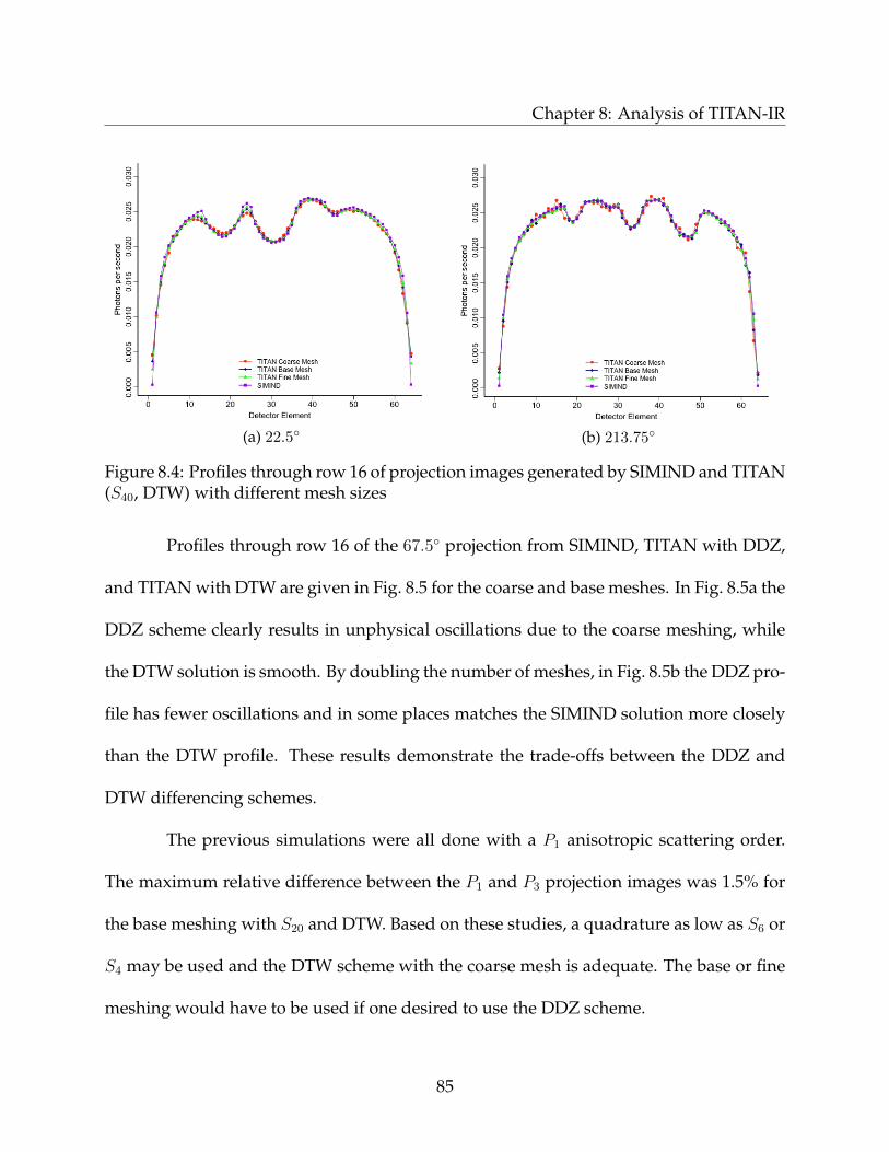
Chapter 8: Analysis of TITAN-IR
(a) 22.5 (b) 213.75
Figure 8.4: Profiles through row 16 of projection images generated by SIMIND and TITAN(S40, DTW) with different mesh sizes
Profiles through row 16 of the 67.5 projection from SIMIND, TITAN with DDZ,
and TITAN with DTW are given in Fig. 8.5 for the coarse and base meshes. In Fig. 8.5a the
DDZ scheme clearly results in unphysical oscillations due to the coarse meshing, while
the DTW solution is smooth. By doubling the number of meshes, in Fig. 8.5b the DDZ pro-
file has fewer oscillations and in some places matches the SIMIND solution more closely
than the DTW profile. These results demonstrate the trade-offs between the DDZ and
DTW differencing schemes.
The previous simulations were all done with a P1 anisotropic scattering order.
The maximum relative difference between the P1 and P3 projection images was 1.5% for
the base meshing with S20 and DTW. Based on these studies, a quadrature as low as S6 or
S4 may be used and the DTW scheme with the coarse mesh is adequate. The base or fine
meshing would have to be used if one desired to use the DDZ scheme.
85
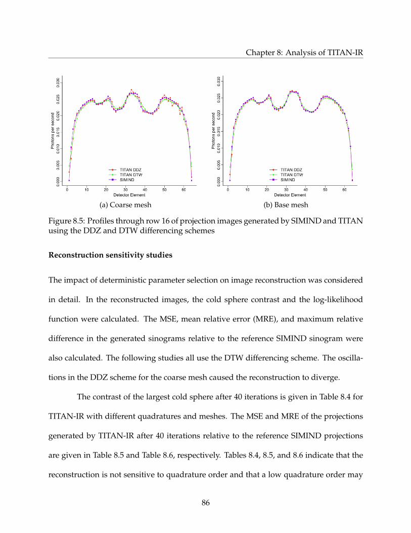
Chapter 8: Analysis of TITAN-IR
(a) Coarse mesh (b) Base mesh
Figure 8.5: Profiles through row 16 of projection images generated by SIMIND and TITANusing the DDZ and DTW differencing schemes
Reconstruction sensitivity studies
The impact of deterministic parameter selection on image reconstruction was considered
in detail. In the reconstructed images, the cold sphere contrast and the log-likelihood
function were calculated. The MSE, mean relative error (MRE), and maximum relative
difference in the generated sinograms relative to the reference SIMIND sinogram were
also calculated. The following studies all use the DTW differencing scheme. The oscilla-
tions in the DDZ scheme for the coarse mesh caused the reconstruction to diverge.
The contrast of the largest cold sphere after 40 iterations is given in Table 8.4 for
TITAN-IR with different quadratures and meshes. The MSE and MRE of the projections
generated by TITAN-IR after 40 iterations relative to the reference SIMIND projections
are given in Table 8.5 and Table 8.6, respectively. Tables 8.4, 8.5, and 8.6 indicate that the
reconstruction is not sensitive to quadrature order and that a low quadrature order may
86
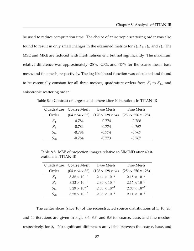
Chapter 8: Analysis of TITAN-IR
be used to reduce computation time. The choice of anisotropic scattering order was also
found to result in only small changes in the examined metrics for P0, P1, P3, and P5. The
MSE and MRE are reduced with mesh refinement, but not significantly. The maximum
relative difference was approximately -25%, -20%, and -17% for the coarse mesh, base
mesh, and fine mesh, respectively. The log-likelihood function was calculated and found
to be essentially constant for all three meshes, quadrature orders from S4 to S40, and
anisotropic scattering order.
Table 8.4: Contrast of largest cold sphere after 40 iterations in TITAN-IR
Quadrature Coarse Mesh Base Mesh Fine MeshOrder (64 x 64 x 32) (128 x 128 x 64) (256 x 256 x 128)
S4 -0.784 -0.774 -0.768S6 -0.784 -0.774 -0.767S14 -0.784 -0.774 -0.767S28 -0.784 -0.773 -0.767
Table 8.5: MSE of projection images relative to SIMIND after 40 it-erations in TITAN-IR
Quadrature Coarse Mesh Base Mesh Fine MeshOrder (64 x 64 x 32) (128 x 128 x 64) (256 x 256 x 128)
S4 3.38× 10⁻⁷ 2.44× 10⁻⁷ 2.18× 10⁻⁷
S6 3.32× 10⁻⁷ 2.39× 10⁻⁷ 2.15× 10⁻⁷
S14 3.29× 10⁻⁷ 2.36× 10⁻⁷ 2.36× 10⁻⁷
S28 3.28× 10⁻⁷ 2.35× 10⁻⁷ 2.11× 10⁻⁷
The center slices (slice 16) of the reconstructed source distributions at 5, 10, 20,
and 40 iterations are given in Figs. 8.6, 8.7, and 8.8 for coarse, base, and fine meshes,
respectively, for S6. No significant differences are visible between the coarse, base, and
87
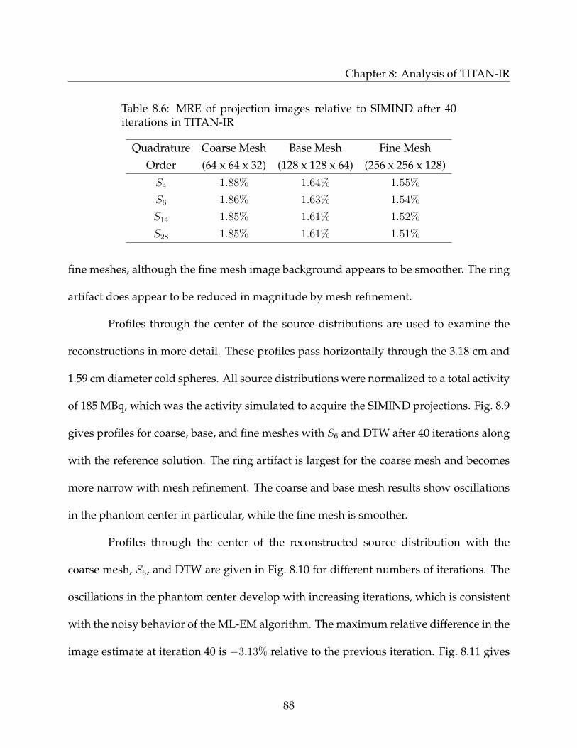
Chapter 8: Analysis of TITAN-IR
Table 8.6: MRE of projection images relative to SIMIND after 40iterations in TITAN-IR
Quadrature Coarse Mesh Base Mesh Fine MeshOrder (64 x 64 x 32) (128 x 128 x 64) (256 x 256 x 128)
S4 1.88% 1.64% 1.55%
S6 1.86% 1.63% 1.54%
S14 1.85% 1.61% 1.52%
S28 1.85% 1.61% 1.51%
fine meshes, although the fine mesh image background appears to be smoother. The ring
artifact does appear to be reduced in magnitude by mesh refinement.
Profiles through the center of the source distributions are used to examine the
reconstructions in more detail. These profiles pass horizontally through the 3.18 cm and
1.59 cm diameter cold spheres. All source distributions were normalized to a total activity
of 185 MBq, which was the activity simulated to acquire the SIMIND projections. Fig. 8.9
gives profiles for coarse, base, and fine meshes with S6 and DTW after 40 iterations along
with the reference solution. The ring artifact is largest for the coarse mesh and becomes
more narrow with mesh refinement. The coarse and base mesh results show oscillations
in the phantom center in particular, while the fine mesh is smoother.
Profiles through the center of the reconstructed source distribution with the
coarse mesh, S6, and DTW are given in Fig. 8.10 for different numbers of iterations. The
oscillations in the phantom center develop with increasing iterations, which is consistent
with the noisy behavior of the ML-EM algorithm. The maximum relative difference in the
image estimate at iteration 40 is −3.13% relative to the previous iteration. Fig. 8.11 gives
88
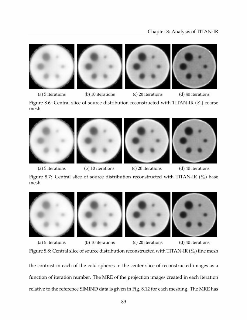
Chapter 8: Analysis of TITAN-IR
(a) 5 iterations (b) 10 iterations (c) 20 iterations (d) 40 iterations
Figure 8.6: Central slice of source distribution reconstructed with TITAN-IR (S6) coarsemesh
(a) 5 iterations (b) 10 iterations (c) 20 iterations (d) 40 iterations
Figure 8.7: Central slice of source distribution reconstructed with TITAN-IR (S6) basemesh
(a) 5 iterations (b) 10 iterations (c) 20 iterations (d) 40 iterations
Figure 8.8: Central slice of source distribution reconstructed with TITAN-IR (S6) fine mesh
the contrast in each of the cold spheres in the center slice of reconstructed images as a
function of iteration number. The MRE of the projection images created in each iteration
relative to the reference SIMIND data is given in Fig. 8.12 for each meshing. The MRE has
89
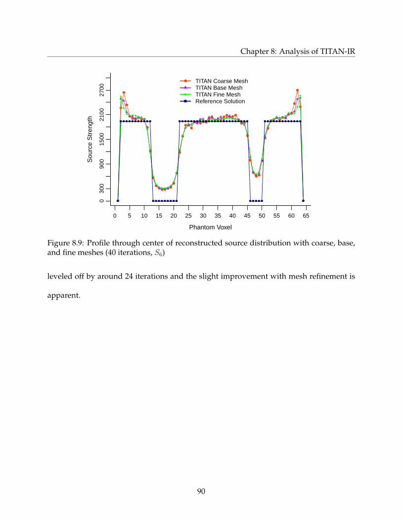
Chapter 8: Analysis of TITAN-IR
0 5 10 15 20 25 30 35 40 45 50 55 60 65
030
090
015
0021
0027
00
Phantom Voxel
Sou
rce
Str
engt
h
Source Distribution
TITAN Coarse MeshTITAN Base MeshTITAN Fine MeshReference Solution
Figure 8.9: Profile through center of reconstructed source distribution with coarse, base,and fine meshes (40 iterations, S6)
leveled off by around 24 iterations and the slight improvement with mesh refinement is
apparent.
90
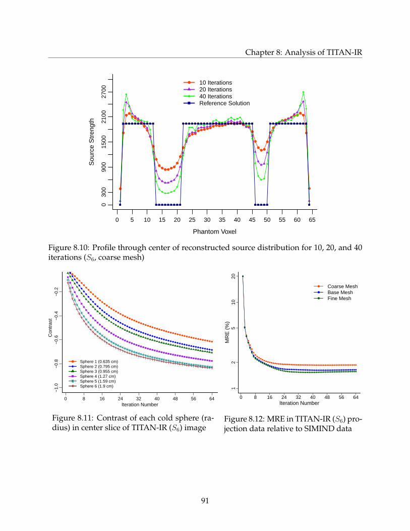
Chapter 8: Analysis of TITAN-IR
0 5 10 15 20 25 30 35 40 45 50 55 60 65
030
090
015
0021
0027
00
Phantom Voxel
Sou
rce
Str
engt
h
Source Distribution
10 Iterations20 Iterations40 IterationsReference Solution
Figure 8.10: Profile through center of reconstructed source distribution for 10, 20, and 40iterations (S6, coarse mesh)
0 8 16 24 32 40 48 56 64
−1.
0−
0.8
−0.
6−
0.4
−0.
20.
0
Iteration Number
Con
tras
t
Sphere 1 (0.635 cm)Sphere 2 (0.795 cm)Sphere 3 (0.955 cm)Sphere 4 (1.27 cm)Sphere 5 (1.59 cm)Sphere 6 (1.9 cm)
Figure 8.11: Contrast of each cold sphere (ra-dius) in center slice of TITAN-IR (S6) image
0 8 16 24 32 40 48 56 64
12
510
20
Iteration Number
MR
E (
%)
Coarse MeshBase MeshFine Mesh
Figure 8.12: MRE in TITAN-IR (S6) pro-jection data relative to SIMIND data
91
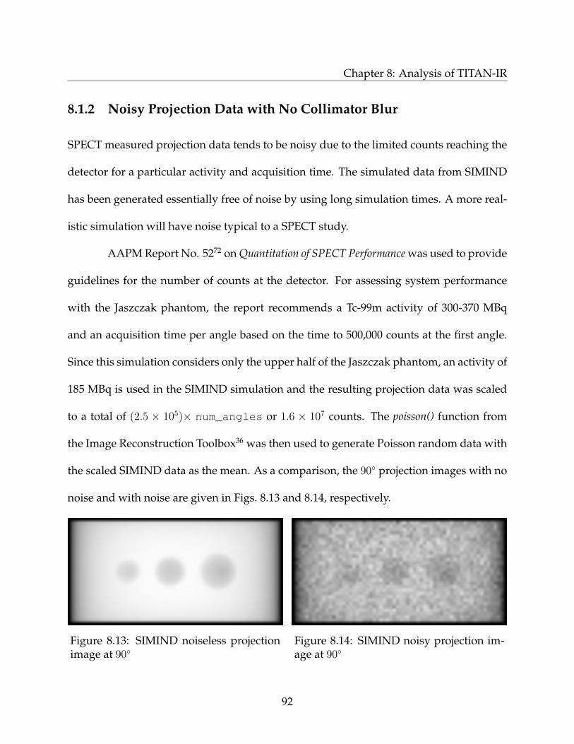
Chapter 8: Analysis of TITAN-IR
8.1.2 Noisy Projection Data with No Collimator Blur
SPECT measured projection data tends to be noisy due to the limited counts reaching the
detector for a particular activity and acquisition time. The simulated data from SIMIND
has been generated essentially free of noise by using long simulation times. A more real-
istic simulation will have noise typical to a SPECT study.
AAPM Report No. 5272 on Quantitation of SPECT Performance was used to provide
guidelines for the number of counts at the detector. For assessing system performance
with the Jaszczak phantom, the report recommends a Tc-99m activity of 300-370 MBq
and an acquisition time per angle based on the time to 500,000 counts at the first angle.
Since this simulation considers only the upper half of the Jaszczak phantom, an activity of
185 MBq is used in the SIMIND simulation and the resulting projection data was scaled
to a total of (2.5 × 10⁵)× num_angles or 1.6 × 10⁷ counts. The poisson() function from
the Image Reconstruction Toolbox36 was then used to generate Poisson random data with
the scaled SIMIND data as the mean. As a comparison, the 90 projection images with no
noise and with noise are given in Figs. 8.13 and 8.14, respectively.
Figure 8.13: SIMIND noiseless projectionimage at 90
Figure 8.14: SIMIND noisy projection im-age at 90
92
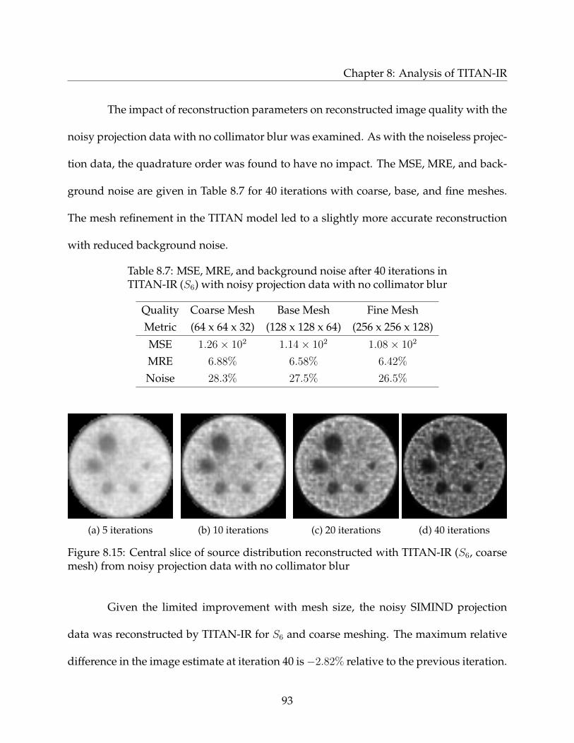
Chapter 8: Analysis of TITAN-IR
The impact of reconstruction parameters on reconstructed image quality with the
noisy projection data with no collimator blur was examined. As with the noiseless projec-
tion data, the quadrature order was found to have no impact. The MSE, MRE, and back-
ground noise are given in Table 8.7 for 40 iterations with coarse, base, and fine meshes.
The mesh refinement in the TITAN model led to a slightly more accurate reconstruction
with reduced background noise.
Table 8.7: MSE, MRE, and background noise after 40 iterations inTITAN-IR (S6) with noisy projection data with no collimator blur
Quality Coarse Mesh Base Mesh Fine MeshMetric (64 x 64 x 32) (128 x 128 x 64) (256 x 256 x 128)
MSE 1.26× 10² 1.14× 10² 1.08× 10²
MRE 6.88% 6.58% 6.42%
Noise 28.3% 27.5% 26.5%
(a) 5 iterations (b) 10 iterations (c) 20 iterations (d) 40 iterations
Figure 8.15: Central slice of source distribution reconstructed with TITAN-IR (S6, coarsemesh) from noisy projection data with no collimator blur
Given the limited improvement with mesh size, the noisy SIMIND projection
data was reconstructed by TITAN-IR for S6 and coarse meshing. The maximum relative
difference in the image estimate at iteration 40 is−2.82% relative to the previous iteration.
93
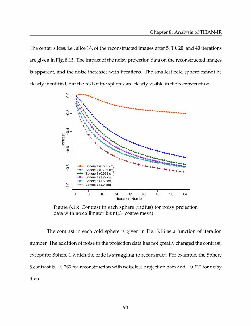
Chapter 8: Analysis of TITAN-IR
The center slices, i.e., slice 16, of the reconstructed images after 5, 10, 20, and 40 iterations
are given in Fig. 8.15. The impact of the noisy projection data on the reconstructed images
is apparent, and the noise increases with iterations. The smallest cold sphere cannot be
clearly identified, but the rest of the spheres are clearly visible in the reconstruction.
0 8 16 24 32 40 48 56 64
−1.
0−
0.8
−0.
6−
0.4
−0.
20.
0
Iteration Number
Con
tras
t
Sphere 1 (0.635 cm)Sphere 2 (0.795 cm)Sphere 3 (0.955 cm)Sphere 4 (1.27 cm)Sphere 5 (1.59 cm)Sphere 6 (1.9 cm)
Figure 8.16: Contrast in each sphere (radius) for noisy projectiondata with no collimator blur (S6, coarse mesh)
The contrast in each cold sphere is given in Fig. 8.16 as a function of iteration
number. The addition of noise to the projection data has not greatly changed the contrast,
except for Sphere 1 which the code is struggling to reconstruct. For example, the Sphere
5 contrast is−0.766 for reconstruction with noiseless projection data and−0.712 for noisy
data.
94
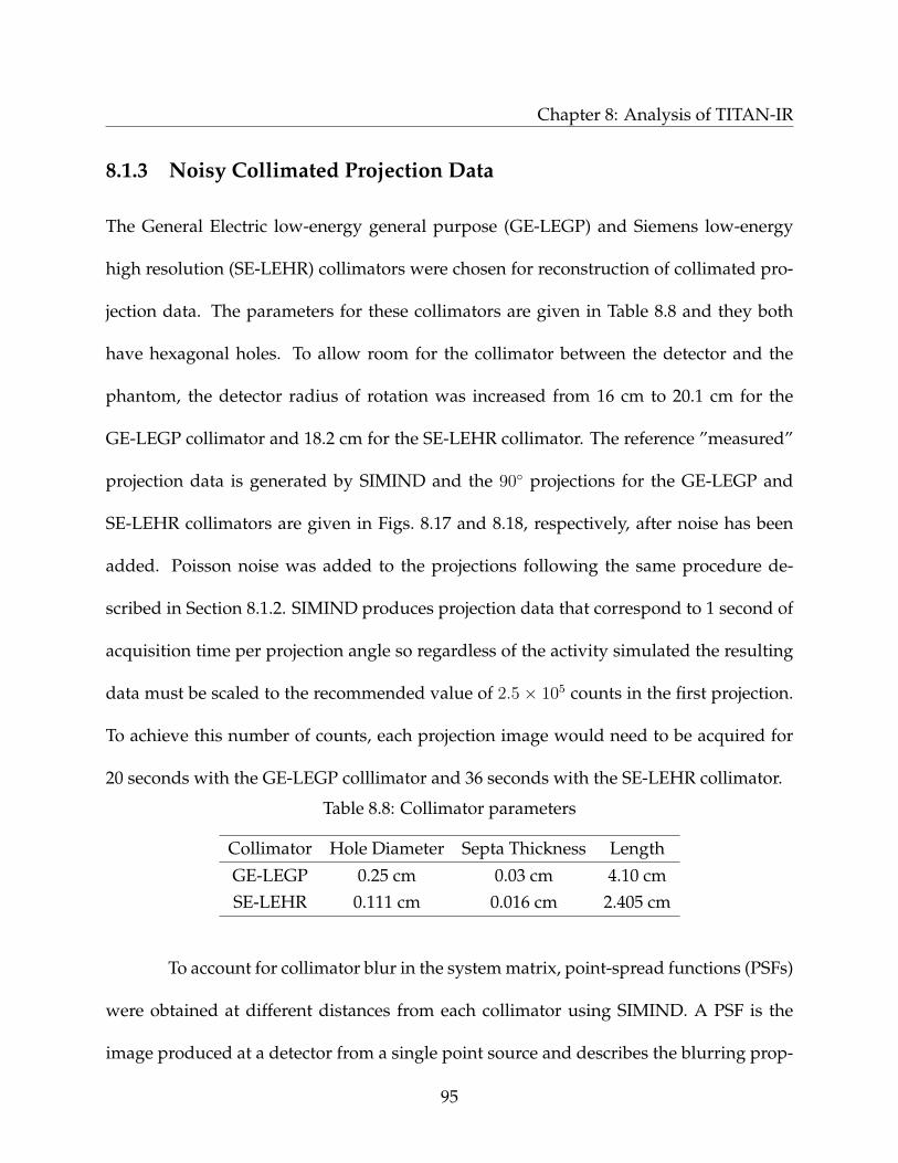
Chapter 8: Analysis of TITAN-IR
8.1.3 Noisy Collimated Projection Data
The General Electric low-energy general purpose (GE-LEGP) and Siemens low-energy
high resolution (SE-LEHR) collimators were chosen for reconstruction of collimated pro-
jection data. The parameters for these collimators are given in Table 8.8 and they both
have hexagonal holes. To allow room for the collimator between the detector and the
phantom, the detector radius of rotation was increased from 16 cm to 20.1 cm for the
GE-LEGP collimator and 18.2 cm for the SE-LEHR collimator. The reference ”measured”
projection data is generated by SIMIND and the 90 projections for the GE-LEGP and
SE-LEHR collimators are given in Figs. 8.17 and 8.18, respectively, after noise has been
added. Poisson noise was added to the projections following the same procedure de-
scribed in Section 8.1.2. SIMIND produces projection data that correspond to 1 second of
acquisition time per projection angle so regardless of the activity simulated the resulting
data must be scaled to the recommended value of 2.5 × 10⁵ counts in the first projection.
To achieve this number of counts, each projection image would need to be acquired for
20 seconds with the GE-LEGP colllimator and 36 seconds with the SE-LEHR collimator.
Table 8.8: Collimator parameters
Collimator Hole Diameter Septa Thickness Length
GE-LEGP 0.25 cm 0.03 cm 4.10 cmSE-LEHR 0.111 cm 0.016 cm 2.405 cm
To account for collimator blur in the system matrix, point-spread functions (PSFs)
were obtained at different distances from each collimator using SIMIND. A PSF is the
image produced at a detector from a single point source and describes the blurring prop-
95
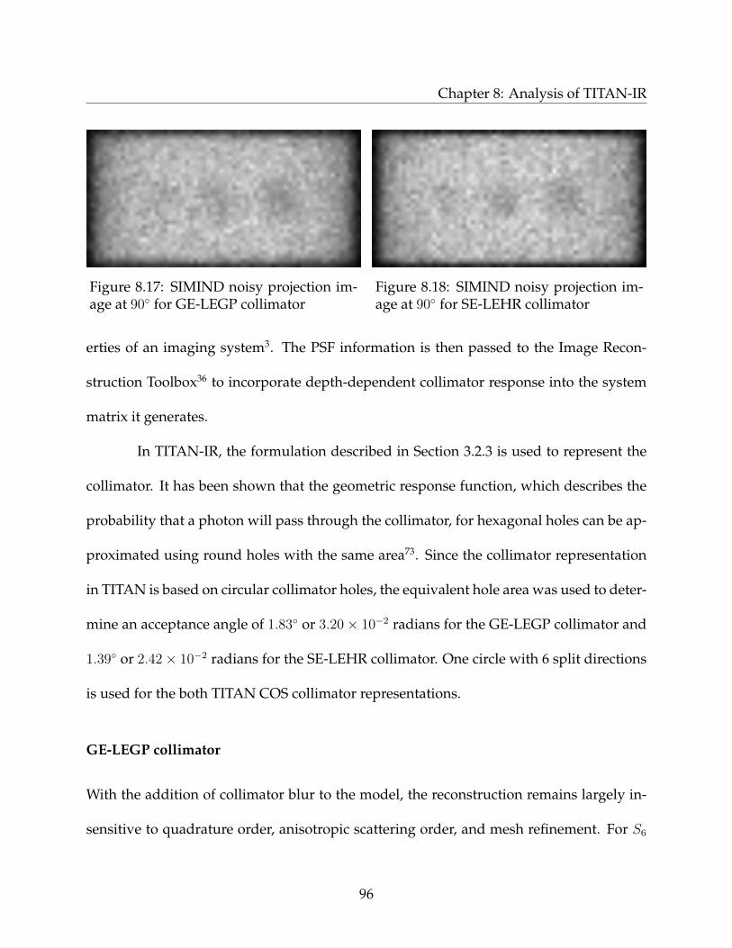
Chapter 8: Analysis of TITAN-IR
Figure 8.17: SIMIND noisy projection im-age at 90 for GE-LEGP collimator
Figure 8.18: SIMIND noisy projection im-age at 90 for SE-LEHR collimator
erties of an imaging system3. The PSF information is then passed to the Image Recon-
struction Toolbox36 to incorporate depth-dependent collimator response into the system
matrix it generates.
In TITAN-IR, the formulation described in Section 3.2.3 is used to represent the
collimator. It has been shown that the geometric response function, which describes the
probability that a photon will pass through the collimator, for hexagonal holes can be ap-
proximated using round holes with the same area73. Since the collimator representation
in TITAN is based on circular collimator holes, the equivalent hole area was used to deter-
mine an acceptance angle of 1.83 or 3.20× 10⁻² radians for the GE-LEGP collimator and
1.39 or 2.42× 10⁻² radians for the SE-LEHR collimator. One circle with 6 split directions
is used for the both TITAN COS collimator representations.
GE-LEGP collimator
With the addition of collimator blur to the model, the reconstruction remains largely in-
sensitive to quadrature order, anisotropic scattering order, and mesh refinement. For S6
96
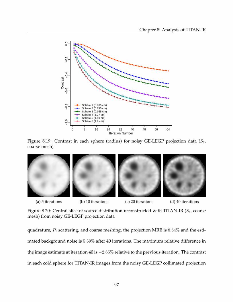
Chapter 8: Analysis of TITAN-IR
0 8 16 24 32 40 48 56 64
−1.
0−
0.8
−0.
6−
0.4
−0.
20.
0
Iteration Number
Con
tras
t
Sphere 1 (0.635 cm)Sphere 2 (0.795 cm)Sphere 3 (0.955 cm)Sphere 4 (1.27 cm)Sphere 5 (1.59 cm)Sphere 6 (1.9 cm)
Figure 8.19: Contrast in each sphere (radius) for noisy GE-LEGP projection data (S6,coarse mesh)
(a) 5 iterations (b) 10 iterations (c) 20 iterations (d) 40 iterations
Figure 8.20: Central slice of source distribution reconstructed with TITAN-IR (S6, coarsemesh) from noisy GE-LEGP projection data
quadrature, P1 scattering, and coarse meshing, the projection MRE is 8.64% and the esti-
mated background noise is 5.59% after 40 iterations. The maximum relative difference in
the image estimate at iteration 40 is−2.65% relative to the previous iteration. The contrast
in each cold sphere for TITAN-IR images from the noisy GE-LEGP collimated projection
97
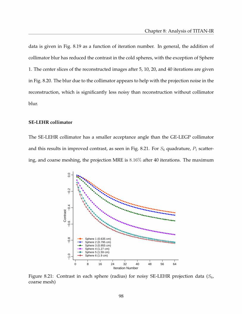
Chapter 8: Analysis of TITAN-IR
data is given in Fig. 8.19 as a function of iteration number. In general, the addition of
collimator blur has reduced the contrast in the cold spheres, with the exception of Sphere
1. The center slices of the reconstructed images after 5, 10, 20, and 40 iterations are given
in Fig. 8.20. The blur due to the collimator appears to help with the projection noise in the
reconstruction, which is significantly less noisy than reconstruction without collimator
blur.
SE-LEHR collimator
The SE-LEHR collimator has a smaller acceptance angle than the GE-LEGP collimator
and this results in improved contrast, as seen in Fig. 8.21. For S6 quadrature, P1 scatter-
ing, and coarse meshing, the projection MRE is 8.16% after 40 iterations. The maximum
0 8 16 24 32 40 48 56 64
−1.
0−
0.8
−0.
6−
0.4
−0.
20.
0
Iteration Number
Con
tras
t
Sphere 1 (0.635 cm)Sphere 2 (0.795 cm)Sphere 3 (0.955 cm)Sphere 4 (1.27 cm)Sphere 5 (1.59 cm)Sphere 6 (1.9 cm)
Figure 8.21: Contrast in each sphere (radius) for noisy SE-LEHR projection data (S6,coarse mesh)
98
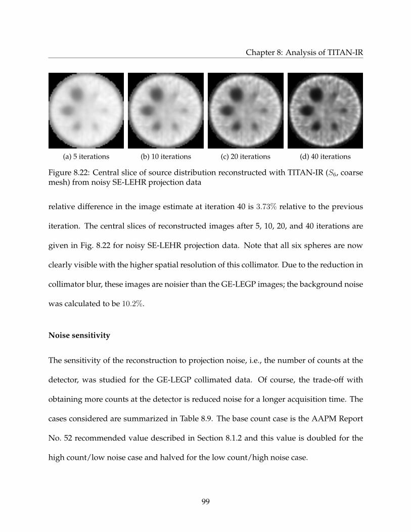
Chapter 8: Analysis of TITAN-IR
(a) 5 iterations (b) 10 iterations (c) 20 iterations (d) 40 iterations
Figure 8.22: Central slice of source distribution reconstructed with TITAN-IR (S6, coarsemesh) from noisy SE-LEHR projection data
relative difference in the image estimate at iteration 40 is 3.73% relative to the previous
iteration. The central slices of reconstructed images after 5, 10, 20, and 40 iterations are
given in Fig. 8.22 for noisy SE-LEHR projection data. Note that all six spheres are now
clearly visible with the higher spatial resolution of this collimator. Due to the reduction in
collimator blur, these images are noisier than the GE-LEGP images; the background noise
was calculated to be 10.2%.
Noise sensitivity
The sensitivity of the reconstruction to projection noise, i.e., the number of counts at the
detector, was studied for the GE-LEGP collimated data. Of course, the trade-off with
obtaining more counts at the detector is reduced noise for a longer acquisition time. The
cases considered are summarized in Table 8.9. The base count case is the AAPM Report
No. 52 recommended value described in Section 8.1.2 and this value is doubled for the
high count/low noise case and halved for the low count/high noise case.
99
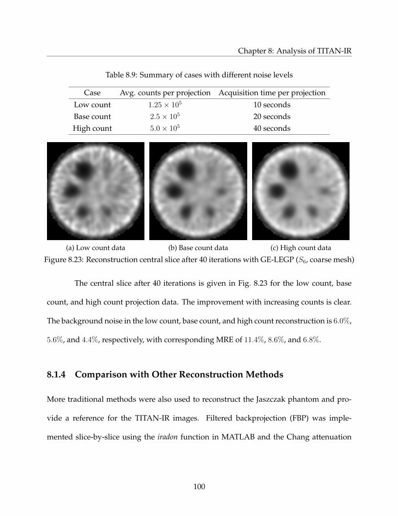
Chapter 8: Analysis of TITAN-IR
Table 8.9: Summary of cases with different noise levels
Case Avg. counts per projection Acquisition time per projection
Low count 1.25× 10⁵ 10 secondsBase count 2.5× 10⁵ 20 secondsHigh count 5.0× 10⁵ 40 seconds
(a) Low count data (b) Base count data (c) High count data
Figure 8.23: Reconstruction central slice after 40 iterations with GE-LEGP (S6, coarse mesh)
The central slice after 40 iterations is given in Fig. 8.23 for the low count, base
count, and high count projection data. The improvement with increasing counts is clear.
The background noise in the low count, base count, and high count reconstruction is 6.0%,
5.6%, and 4.4%, respectively, with corresponding MRE of 11.4%, 8.6%, and 6.8%.
8.1.4 Comparison with Other Reconstruction Methods
More traditional methods were also used to reconstruct the Jaszczak phantom and pro-
vide a reference for the TITAN-IR images. Filtered backprojection (FBP) was imple-
mented slice-by-slice using the iradon function in MATLAB and the Chang attenuation
100
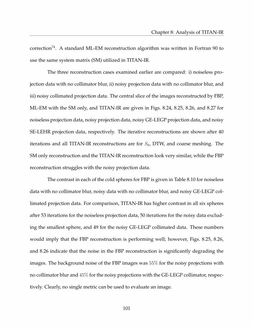
Chapter 8: Analysis of TITAN-IR
correction74. A standard ML-EM reconstruction algorithm was written in Fortran 90 to
use the same system matrix (SM) utilized in TITAN-IR.
The three reconstruction cases examined earlier are compared: i) noiseless pro-
jection data with no collimator blur, ii) noisy projection data with no collimator blur, and
iii) noisy collimated projection data. The central slice of the images reconstructed by FBP,
ML-EM with the SM only, and TITAN-IR are given in Figs. 8.24, 8.25, 8.26, and 8.27 for
noiseless projection data, noisy projection data, noisy GE-LEGP projection data, and noisy
SE-LEHR projection data, respectively. The iterative reconstructions are shown after 40
iterations and all TITAN-IR reconstructions are for S6, DTW, and coarse meshing. The
SM only reconstruction and the TITAN-IR reconstruction look very similar, while the FBP
reconstruction struggles with the noisy projection data.
The contrast in each of the cold spheres for FBP is given in Table 8.10 for noiseless
data with no collimator blur, noisy data with no collimator blur, and noisy GE-LEGP col-
limated projection data. For comparison, TITAN-IR has higher contrast in all six spheres
after 53 iterations for the noiseless projection data, 50 iterations for the noisy data exclud-
ing the smallest sphere, and 49 for the noisy GE-LEGP collimated data. These numbers
would imply that the FBP reconstruction is performing well; however, Figs. 8.25, 8.26,
and 8.26 indicate that the noise in the FBP reconstruction is significantly degrading the
images. The background noise of the FBP images was 55% for the noisy projections with
no collimator blur and 45% for the noisy projections with the GE-LEGP collimator, respec-
tively. Clearly, no single metric can be used to evaluate an image.
101

Chapter 8: Analysis of TITAN-IR
(a) Filtered backprojection (b) System matrix only (c) TITAN-IR
Figure 8.24: Central slice of reconstruction of noiseless projection data
(a) Filtered backprojection (b) System matrix only (c) TITAN-IR
Figure 8.25: Central slice of reconstruction of noisy projection data
(a) Filtered backprojection (b) System matrix only (c) TITAN-IR
Figure 8.26: Central slice of reconstruction of noisy GE-LEGP collimator projection data
102
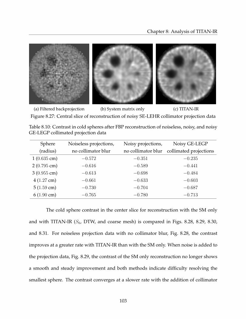
Chapter 8: Analysis of TITAN-IR
(a) Filtered backprojection (b) System matrix only (c) TITAN-IR
Figure 8.27: Central slice of reconstruction of noisy SE-LEHR collimator projection data
Table 8.10: Contrast in cold spheres after FBP reconstruction of noiseless, noisy, and noisyGE-LEGP collimated projection data
Sphere Noiseless projections, Noisy projections, Noisy GE-LEGP(radius) no collimator blur no collimator blur collimated projections
1 (0.635 cm) −0.572 −0.351 −0.235
2 (0.795 cm) −0.616 −0.589 −0.441
3 (0.955 cm) −0.613 −0.698 −0.484
4 (1.27 cm) −0.661 −0.633 −0.603
5 (1.59 cm) −0.730 −0.704 −0.687
6 (1.90 cm) −0.765 −0.780 −0.713
The cold sphere contrast in the center slice for reconstruction with the SM only
and with TITAN-IR (S6, DTW, and coarse mesh) is compared in Figs. 8.28, 8.29, 8.30,
and 8.31. For noiseless projection data with no collimator blur, Fig. 8.28, the contrast
improves at a greater rate with TITAN-IR than with the SM only. When noise is added to
the projection data, Fig. 8.29, the contrast of the SM only reconstruction no longer shows
a smooth and steady improvement and both methods indicate difficulty resolving the
smallest sphere. The contrast converges at a slower rate with the addition of collimator
103
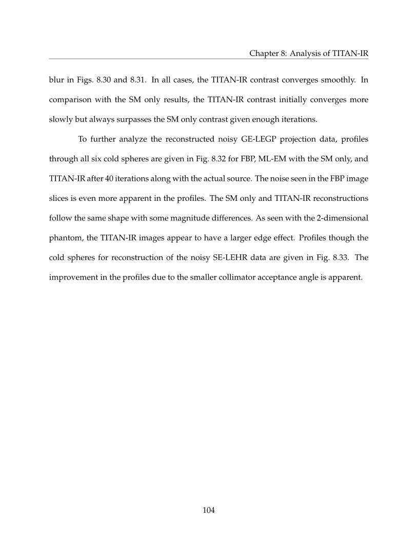
Chapter 8: Analysis of TITAN-IR
blur in Figs. 8.30 and 8.31. In all cases, the TITAN-IR contrast converges smoothly. In
comparison with the SM only results, the TITAN-IR contrast initially converges more
slowly but always surpasses the SM only contrast given enough iterations.
To further analyze the reconstructed noisy GE-LEGP projection data, profiles
through all six cold spheres are given in Fig. 8.32 for FBP, ML-EM with the SM only, and
TITAN-IR after 40 iterations along with the actual source. The noise seen in the FBP image
slices is even more apparent in the profiles. The SM only and TITAN-IR reconstructions
follow the same shape with some magnitude differences. As seen with the 2-dimensional
phantom, the TITAN-IR images appear to have a larger edge effect. Profiles though the
cold spheres for reconstruction of the noisy SE-LEHR data are given in Fig. 8.33. The
improvement in the profiles due to the smaller collimator acceptance angle is apparent.
104
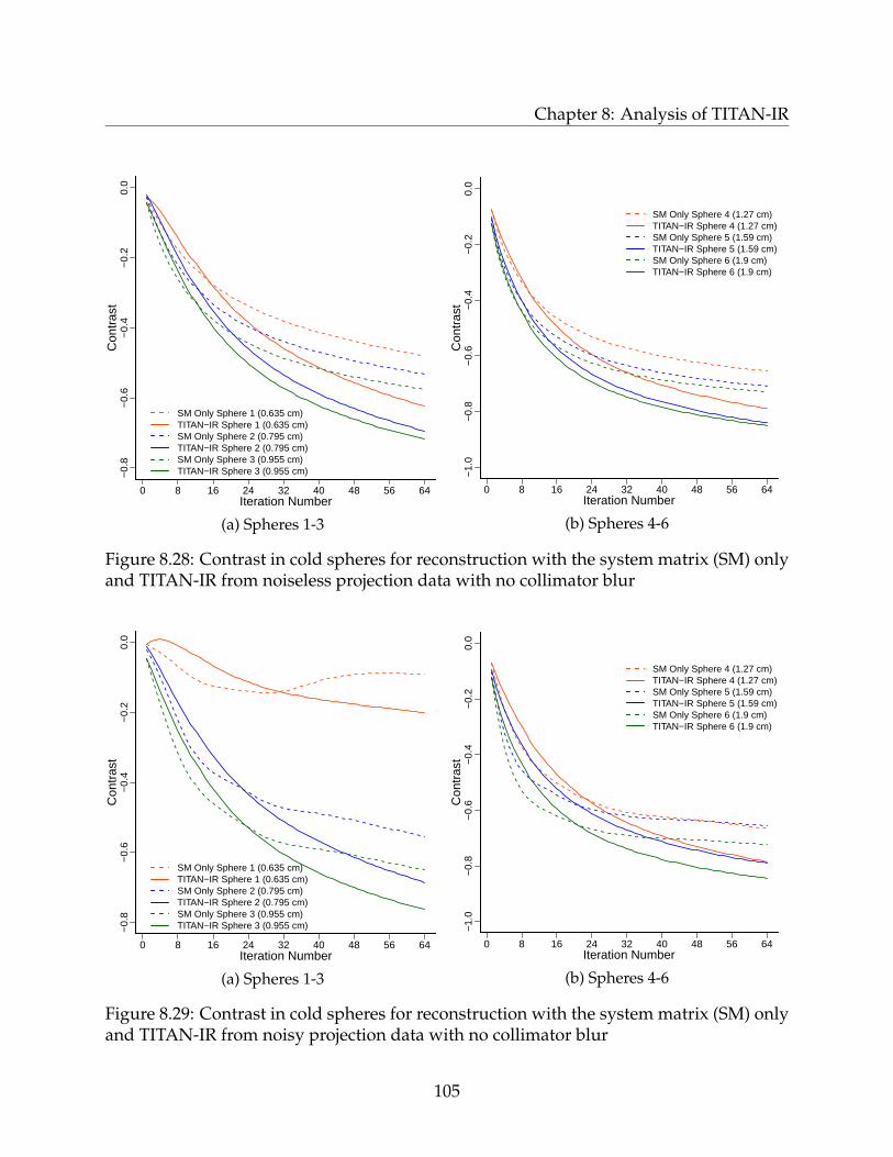
Chapter 8: Analysis of TITAN-IR
0 8 16 24 32 40 48 56 64
−0.
8−
0.6
−0.
4−
0.2
0.0
Iteration Number
Con
tras
t
SM Only Sphere 1 (0.635 cm)TITAN−IR Sphere 1 (0.635 cm)SM Only Sphere 2 (0.795 cm)TITAN−IR Sphere 2 (0.795 cm)SM Only Sphere 3 (0.955 cm)TITAN−IR Sphere 3 (0.955 cm)
(a) Spheres 1-3
0 8 16 24 32 40 48 56 64
−1.
0−
0.8
−0.
6−
0.4
−0.
20.
0
Iteration Number
Con
tras
t
SM Only Sphere 4 (1.27 cm)TITAN−IR Sphere 4 (1.27 cm)SM Only Sphere 5 (1.59 cm)TITAN−IR Sphere 5 (1.59 cm)SM Only Sphere 6 (1.9 cm)TITAN−IR Sphere 6 (1.9 cm)
(b) Spheres 4-6
Figure 8.28: Contrast in cold spheres for reconstruction with the system matrix (SM) onlyand TITAN-IR from noiseless projection data with no collimator blur
0 8 16 24 32 40 48 56 64
−0.
8−
0.6
−0.
4−
0.2
0.0
Iteration Number
Con
tras
t
SM Only Sphere 1 (0.635 cm)TITAN−IR Sphere 1 (0.635 cm)SM Only Sphere 2 (0.795 cm)TITAN−IR Sphere 2 (0.795 cm)SM Only Sphere 3 (0.955 cm)TITAN−IR Sphere 3 (0.955 cm)
(a) Spheres 1-3
0 8 16 24 32 40 48 56 64
−1.
0−
0.8
−0.
6−
0.4
−0.
20.
0
Iteration Number
Con
tras
t
SM Only Sphere 4 (1.27 cm)TITAN−IR Sphere 4 (1.27 cm)SM Only Sphere 5 (1.59 cm)TITAN−IR Sphere 5 (1.59 cm)SM Only Sphere 6 (1.9 cm)TITAN−IR Sphere 6 (1.9 cm)
(b) Spheres 4-6
Figure 8.29: Contrast in cold spheres for reconstruction with the system matrix (SM) onlyand TITAN-IR from noisy projection data with no collimator blur
105
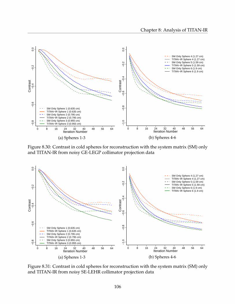
Chapter 8: Analysis of TITAN-IR
0 8 16 24 32 40 48 56 64
−0.
8−
0.6
−0.
4−
0.2
0.0
Iteration Number
Con
tras
t
SM Only Sphere 1 (0.635 cm)TITAN−IR Sphere 1 (0.635 cm)SM Only Sphere 2 (0.795 cm)TITAN−IR Sphere 2 (0.795 cm)SM Only Sphere 3 (0.955 cm)TITAN−IR Sphere 3 (0.955 cm)
(a) Spheres 1-3
0 8 16 24 32 40 48 56 64
−1.
0−
0.8
−0.
6−
0.4
−0.
20.
0
Iteration Number
Con
tras
t
SM Only Sphere 4 (1.27 cm)TITAN−IR Sphere 4 (1.27 cm)SM Only Sphere 5 (1.59 cm)TITAN−IR Sphere 5 (1.59 cm)SM Only Sphere 6 (1.9 cm)TITAN−IR Sphere 6 (1.9 cm)
(b) Spheres 4-6
Figure 8.30: Contrast in cold spheres for reconstruction with the system matrix (SM) onlyand TITAN-IR from noisy GE-LEGP collimator projection data
0 8 16 24 32 40 48 56 64
−0.
8−
0.6
−0.
4−
0.2
0.0
Iteration Number
Con
tras
t
SM Only Sphere 1 (0.635 cm)TITAN−IR Sphere 1 (0.635 cm)SM Only Sphere 2 (0.795 cm)TITAN−IR Sphere 2 (0.795 cm)SM Only Sphere 3 (0.955 cm)TITAN−IR Sphere 3 (0.955 cm)
(a) Spheres 1-3
0 8 16 24 32 40 48 56 64
−1.
0−
0.8
−0.
6−
0.4
−0.
20.
0
Iteration Number
Con
tras
t
SM Only Sphere 4 (1.27 cm)TITAN−IR Sphere 4 (1.27 cm)SM Only Sphere 5 (1.59 cm)TITAN−IR Sphere 5 (1.59 cm)SM Only Sphere 6 (1.9 cm)TITAN−IR Sphere 6 (1.9 cm)
(b) Spheres 4-6
Figure 8.31: Contrast in cold spheres for reconstruction with the system matrix (SM) onlyand TITAN-IR from noisy SE-LEHR collimator projection data
106
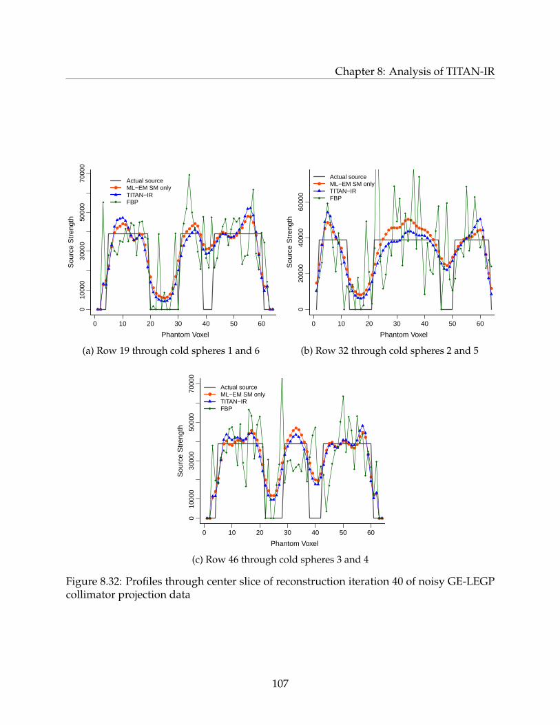
Chapter 8: Analysis of TITAN-IR
0 10 20 30 40 50 60
010
000
3000
050
000
7000
0
Phantom Voxel
Sou
rce
Str
engt
h
Noisy GE−LEGP Data Row 19
Actual sourceML−EM SM onlyTITAN−IRFBP
(a) Row 19 through cold spheres 1 and 6
0 10 20 30 40 50 60
020
000
4000
060
000
Phantom Voxel
Sou
rce
Str
engt
h
Noisy GE−LEGP Data Row 32
Actual sourceML−EM SM onlyTITAN−IRFBP
(b) Row 32 through cold spheres 2 and 5
0 10 20 30 40 50 60
010
000
3000
050
000
7000
0
Phantom Voxel
Sou
rce
Str
engt
h
Noisy GE−LEGP Data Row 46
Actual sourceML−EM SM onlyTITAN−IRFBP
(c) Row 46 through cold spheres 3 and 4
Figure 8.32: Profiles through center slice of reconstruction iteration 40 of noisy GE-LEGPcollimator projection data
107

Chapter 8: Analysis of TITAN-IR
0 10 20 30 40 50 60
050
000
1000
0015
0000
Phantom Voxel
Sou
rce
Str
engt
h
Noisy SE−LEHR Data Row 19
Actual sourceML−EM SM onlyTITAN−IRFBP
(a) Row 19 through cold spheres 1 and 6
0 10 20 30 40 50 60
020
000
6000
010
0000
Phantom Voxel
Sou
rce
Str
engt
h
Noisy SE−LEHR Data Row 32
Actual sourceML−EM SM onlyTITAN−IRFBP
(b) Row 32 through cold spheres 2 and 5
0 10 20 30 40 50 60
020
000
6000
010
0000
Phantom Voxel
Sou
rce
Str
engt
h
Noisy SE−LEHR Data Row 46
Actual sourceML−EM SM onlyTITAN−IRFBP
(c) Row 46 through cold spheres 3 and 4
Figure 8.33: Profiles through center slice of reconstruction iteration 40 of noisy SE-LEHRcollimator projection data
108

Chapter 8: Analysis of TITAN-IR
8.1.5 Computation Time
The computation time for reconstruction with TITAN-IR is an important factor in its per-
formance. The TITAN code was already an efficient parallel transport code and all at-
tempts have been made for TITAN-IR to be fully parallelized. In the following sections,
the computation times to reconstruct the Jaszczak phantom and the possibility for im-
provement through the use of ordered-subsets expectation-maximization (OS-EM) are
examined. All calculations are completed on a dedicated computer cluster with Intel
Xeon E5 2.6 GHz processors, 16 GB of memory per processor core, and 16 processor cores
per compute node. The value of 64 iterations is used so that the number of total iterations
can be scaled with increasing subsets for OS-EM.
ML-EM computation time
The time to complete 64 iterations on noiseless projection data with no collimator blur
for the coarse, base, and fine meshes is given in Table 8.11. The computation times scale
closely with the number of meshes in the model. The computation time for noisy projec-
tion data with no collimator blur is the same as the noiseless case. The system matrix for
the noisy GE-LEGP collimator projection data is much less sparse, i.e., larger, and so the
computation time is 172 s for that case with base meshing. The computation time could be
minimized by reducing the system matrix size, i.e., eliminating values below a threshold.
The computation times and parallel speedup for varying numbers of processor
cores are given in Table 8.12 for projection data with no collimator blur and in Table 8.13
109
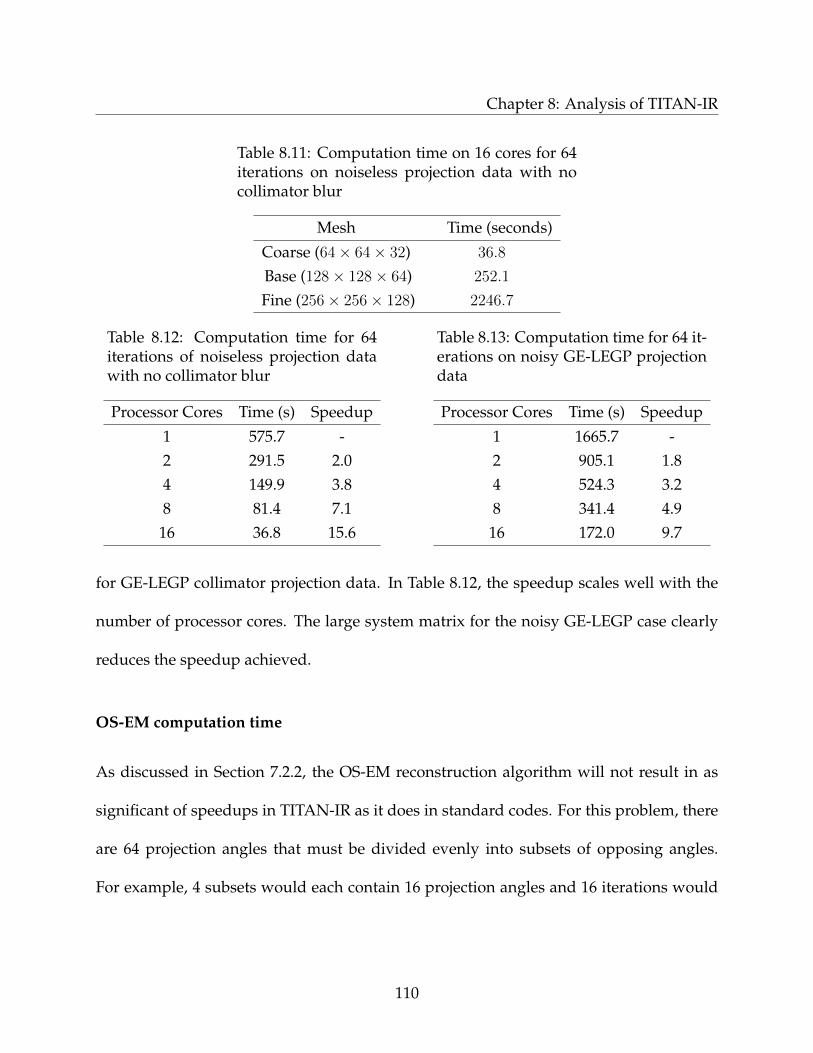
Chapter 8: Analysis of TITAN-IR
Table 8.11: Computation time on 16 cores for 64iterations on noiseless projection data with nocollimator blur
Mesh Time (seconds)
Coarse (64× 64× 32) 36.8
Base (128× 128× 64) 252.1
Fine (256× 256× 128) 2246.7
Table 8.12: Computation time for 64iterations of noiseless projection datawith no collimator blur
Processor Cores Time (s) Speedup
1 575.7 -2 291.5 2.04 149.9 3.88 81.4 7.1
16 36.8 15.6
Table 8.13: Computation time for 64 it-erations on noisy GE-LEGP projectiondata
Processor Cores Time (s) Speedup
1 1665.7 -2 905.1 1.84 524.3 3.28 341.4 4.9
16 172.0 9.7
for GE-LEGP collimator projection data. In Table 8.12, the speedup scales well with the
number of processor cores. The large system matrix for the noisy GE-LEGP case clearly
reduces the speedup achieved.
OS-EM computation time
As discussed in Section 7.2.2, the OS-EM reconstruction algorithm will not result in as
significant of speedups in TITAN-IR as it does in standard codes. For this problem, there
are 64 projection angles that must be divided evenly into subsets of opposing angles.
For example, 4 subsets would each contain 16 projection angles and 16 iterations would
110
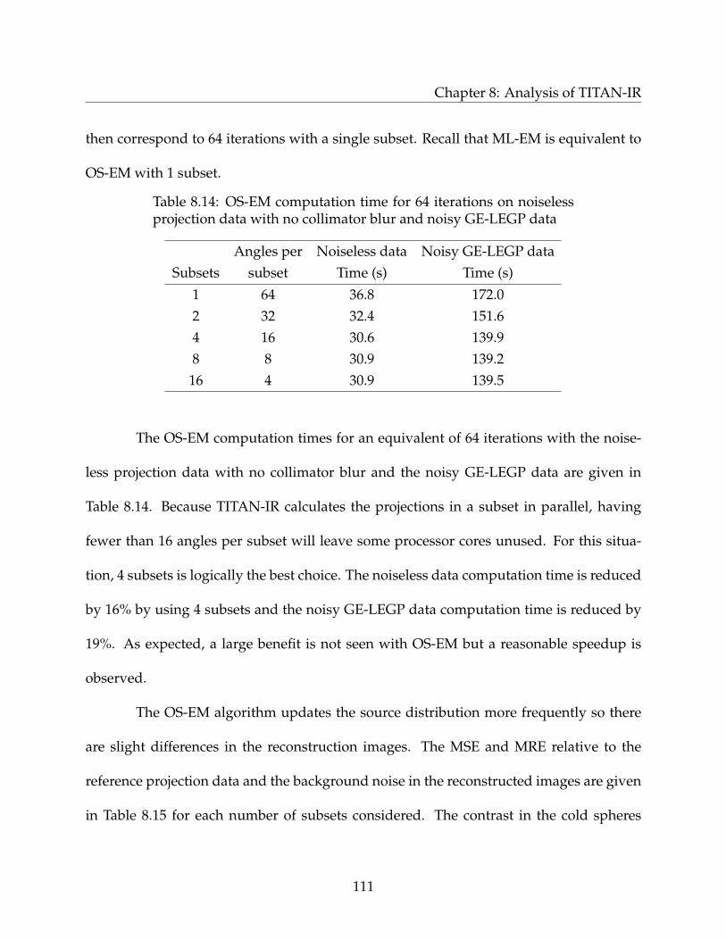
Chapter 8: Analysis of TITAN-IR
then correspond to 64 iterations with a single subset. Recall that ML-EM is equivalent to
OS-EM with 1 subset.
Table 8.14: OS-EM computation time for 64 iterations on noiselessprojection data with no collimator blur and noisy GE-LEGP data
Angles per Noiseless data Noisy GE-LEGP dataSubsets subset Time (s) Time (s)
1 64 36.8 172.02 32 32.4 151.64 16 30.6 139.98 8 30.9 139.2
16 4 30.9 139.5
The OS-EM computation times for an equivalent of 64 iterations with the noise-
less projection data with no collimator blur and the noisy GE-LEGP data are given in
Table 8.14. Because TITAN-IR calculates the projections in a subset in parallel, having
fewer than 16 angles per subset will leave some processor cores unused. For this situa-
tion, 4 subsets is logically the best choice. The noiseless data computation time is reduced
by 16% by using 4 subsets and the noisy GE-LEGP data computation time is reduced by
19%. As expected, a large benefit is not seen with OS-EM but a reasonable speedup is
observed.
The OS-EM algorithm updates the source distribution more frequently so there
are slight differences in the reconstruction images. The MSE and MRE relative to the
reference projection data and the background noise in the reconstructed images are given
in Table 8.15 for each number of subsets considered. The contrast in the cold spheres
111

Chapter 8: Analysis of TITAN-IR
after 64 iterations is given in Table 8.16. Only small changes in these metrics are seen for
different numbers of subsets.
Table 8.15: MSE, MRE, and background noise after 64iterations in TITAN-IR with varying number of subsets
Subsets MSE MRE Background Noise
1 1.27× 10² 8.36% 7.26%2 1.26× 10² 8.32% 7.25%4 1.25× 10² 8.30% 7.61%8 1.23× 10² 8.14% 7.20%
16 1.29× 10² 8.32% 7.80%
Table 8.16: Contrast of cold spheres after 64 iterations in TITAN-IR with varyingnumber of subsets
Sphere 1 Sphere 2 Sphere 3 Sphere 4 Sphere 5 Sphere 6Subsets (0.635 cm) (0.795 cm) (0.955 cm) (1.27 cm) (1.59 cm) (1.9 cm)
1 -0.346 -0.510 -0.554 -0.694 -0.783 -0.8092 -0.345 -0.510 -0.553 -0.694 -0.783 -0.8094 -0.351 -0.512 -0.555 -0.695 -0.785 -0.8108 -0.362 -0.512 -0.560 -0.698 -0.791 -0.812
16 -0.345 -0.502 -0.556 -0.698 -0.792 -0.811
8.2 NCAT Phantom
The NURBS-based cardiac-torso (NCAT) phantom61 was used as an anatomical recon-
struction case for testing of TITAN-IR. This heterogeneous phantom includes the fol-
lowing materials: air, body tissue (represented as water), intestine, lung, rib bone, liver,
kidney, spine bone, muscle, cartilage, spleen, heart, and blood. Axial and lateral views of
112
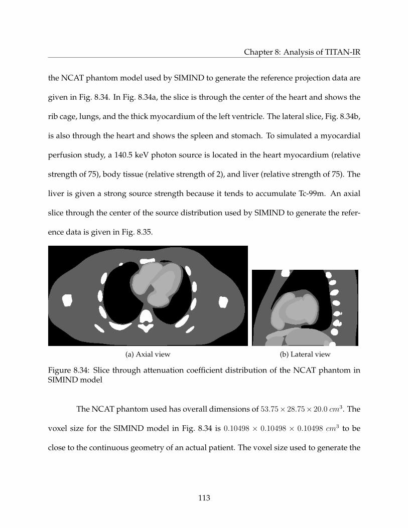
Chapter 8: Analysis of TITAN-IR
the NCAT phantom model used by SIMIND to generate the reference projection data are
given in Fig. 8.34. In Fig. 8.34a, the slice is through the center of the heart and shows the
rib cage, lungs, and the thick myocardium of the left ventricle. The lateral slice, Fig. 8.34b,
is also through the heart and shows the spleen and stomach. To simulated a myocardial
perfusion study, a 140.5 keV photon source is located in the heart myocardium (relative
strength of 75), body tissue (relative strength of 2), and liver (relative strength of 75). The
liver is given a strong source strength because it tends to accumulate Tc-99m. An axial
slice through the center of the source distribution used by SIMIND to generate the refer-
ence data is given in Fig. 8.35.
(a) Axial view (b) Lateral view
Figure 8.34: Slice through attenuation coefficient distribution of the NCAT phantom inSIMIND model
The NCAT phantom used has overall dimensions of 53.75× 28.75× 20.0 cm3. The
voxel size for the SIMIND model in Fig. 8.34 is 0.10498 × 0.10498 × 0.10498 cm3 to be
close to the continuous geometry of an actual patient. The voxel size used to generate the
113
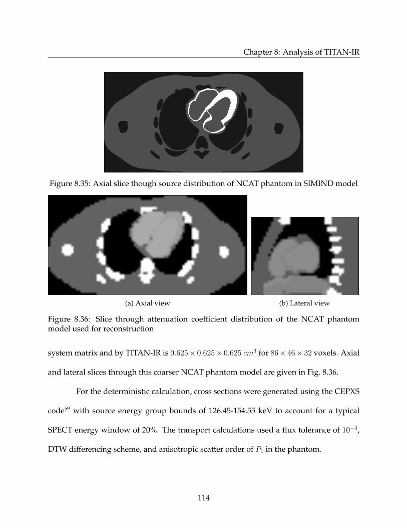
Chapter 8: Analysis of TITAN-IR
Figure 8.35: Axial slice though source distribution of NCAT phantom in SIMIND model
(a) Axial view (b) Lateral view
Figure 8.36: Slice through attenuation coefficient distribution of the NCAT phantommodel used for reconstruction
system matrix and by TITAN-IR is 0.625× 0.625× 0.625 cm3 for 86× 46× 32 voxels. Axial
and lateral slices through this coarser NCAT phantom model are given in Fig. 8.36.
For the deterministic calculation, cross sections were generated using the CEPXS
code59 with source energy group bounds of 126.45-154.55 keV to account for a typical
SPECT energy window of 20%. The transport calculations used a flux tolerance of 10−3,
DTW differencing scheme, and anisotropic scatter order of P1 in the phantom.
114

Chapter 8: Analysis of TITAN-IR
Figure 8.37: Reference frontal projectiondata
Figure 8.38: TITAN-IR frontal projectiondata after 40 iterations
A flat source distribution of one is used for the initial guess of all reconstructions
and the system matrix is obtained using the Image Reconstruction Toolbox36 for MAT-
LAB. The NCAT phantom is reconstructed for the cases of noiseless projection data with
no collimator blur and noisy collimated projection data. For both cases, the performance
of the TITAN-IR code will be evaluated and compared with FBP and ML-EM with SM
only reconstruction.
8.2.1 Noiseless Projection Data with No Collimator Blur
Projection data with no noise or collimator blur was reconstructed first. The reference
frontal projection data is given in Fig. 8.37 and clearly shows the strong source in the
heart wall and liver. The TITAN-IR frontal projection data after 40 iterations is given in
Fig. 8.38. The TITAN-IR projection data agrees well visually.
The MSE and MRE in the projections after 40 iterations relative to the reference
projection data are given in Table 8.17 for increasing quadrature order and the base mesh-
ing. Also given in Table 8.17 is the estimated background noise a region of soft tissue.
At iteration 40, the maximum relative difference in the image estimate is −4.02% rela-
115

Chapter 8: Analysis of TITAN-IR
Table 8.17: MSE, MRE, and back-ground noise after 40 iterations withthe base meshing
SN MSE MRE Noise
S6 5.77× 10⁻⁴ 8.88% 13.4%
S8 5.78× 10⁻⁴ 8.87% 12.2%
S16 5.79× 10⁻⁴ 8.87% 12.4%
Table 8.18: MSE, MRE, and back-ground noise after 40 iterations withthe fine meshing
SN MSE MRE Noise
S6 4.08× 10⁻⁴ 6.57% 10.1%
S8 4.09× 10⁻⁴ 6.56% 9.6%
S16 4.09× 10⁻⁴ 6.56% 9.7%
tive to the previous iteration. The number of meshes in the TITAN model was refined
to 172 × 92 × 64 voxels to create a fine meshing case. With the fine meshing, the MSE
and MRE in the projections after 40 iterations relative to the reference projection data are
given in Table 8.18 for increasing quadrature order along with the estimated background
noise a region of soft tissue. The maximum relative difference in the image estimate at 40
iterations is 2.65% relative to the previous iteration. The quadrature order, i.e., number of
directions in the deterministic model, clearly does not impact the reconstruction signifi-
cantly, although there is a small reduction in noise. Mesh refinement reduces the MRE by
about 2%, but comes at the cost of longer computation time.
Axial and frontal slices through the reconstructed source distribution after 40 it-
erations with S8 quadrature and base meshing are given in Fig. 8.39. Fig. 8.39a is through
the center of the heart and shows the thick myocardium of the left ventricle. In Fig. 8.39b,
the left ventricle is clearly visible as the solid ring of source and the liver is located below
the heart.
As a comparison, the NCAT phantom results are reconstructed with FBP in
Fig. 8.40 and the SM only in Fig. 8.41. The FBP image has streak artifacts in the axial slice,
116
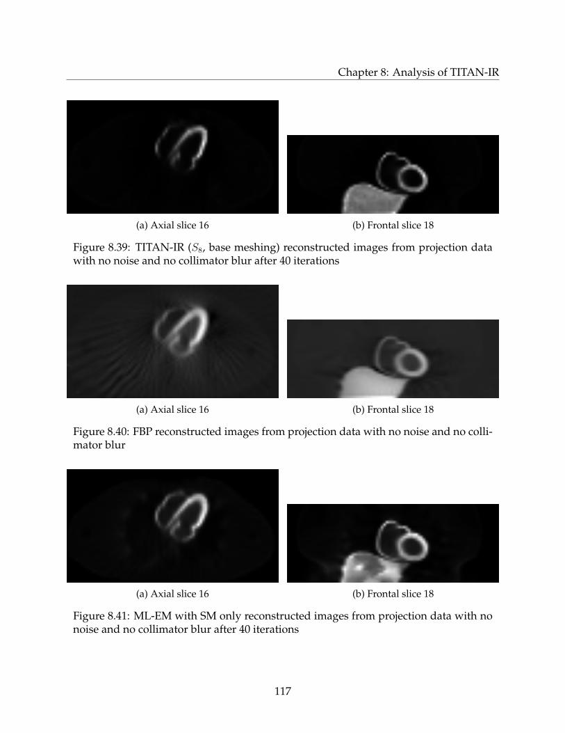
Chapter 8: Analysis of TITAN-IR
(a) Axial slice 16 (b) Frontal slice 18
Figure 8.39: TITAN-IR (S8, base meshing) reconstructed images from projection datawith no noise and no collimator blur after 40 iterations
(a) Axial slice 16 (b) Frontal slice 18
Figure 8.40: FBP reconstructed images from projection data with no noise and no colli-mator blur
(a) Axial slice 16 (b) Frontal slice 18
Figure 8.41: ML-EM with SM only reconstructed images from projection data with nonoise and no collimator blur after 40 iterations
117

Chapter 8: Analysis of TITAN-IR
0 20 40 60 80
050
0000
1000
000
1500
000
2000
000
Phantom Voxel
Sou
rce
Str
engt
h
No Noise Data Row 19 80 iterations
FBPML−EM SM onlyTITAN−IR
(a) Row 19
0 10 20 30 40
050
0000
1000
000
1500
000
2000
000
Phantom Voxel
Sou
rce
Str
engt
h
FBPML−EM SM onlyTITAN−IR
(b) Column 53
Figure 8.42: Profiles through heart after reconstruction iteration 40 of noiseless projectiondata with no collimator blur
but the myocardium is very clear. The SM only image also shows the myocardium well,
but suffers from artifacts in the liver. To further compare reconstruction methods, profiles
through the axial slice are given in Fig. 8.42. The TITAN-IR profile has the largest differ-
entiation between the myocardium and other tissues. In Fig. 8.42a, the FBP and SM only
profiles match well, but in Fig. 8.42b the FBP profile has not resolved the myocardium as
well.
8.2.2 Noisy Collimated Projection Data
To examine the reconstruction of the NCAT phantom with noisy collimated data, the GE-
LEGP collimator described in Section 8.1.3 was used to create the reference projection data
in SIMIND. As explained in Section 8.1.2, Poisson noise was then added to the reference
118
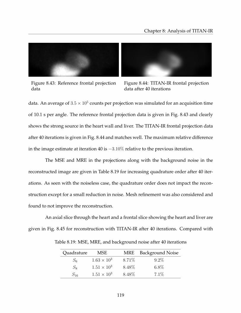
Chapter 8: Analysis of TITAN-IR
Figure 8.43: Reference frontal projectiondata
Figure 8.44: TITAN-IR frontal projectiondata after 40 iterations
data. An average of 3.5× 10⁵ counts per projection was simulated for an acquisition time
of 10.1 s per angle. The reference frontal projection data is given in Fig. 8.43 and clearly
shows the strong source in the heart wall and liver. The TITAN-IR frontal projection data
after 40 iterations is given in Fig. 8.44 and matches well. The maximum relative difference
in the image estimate at iteration 40 is −3.10% relative to the previous iteration.
The MSE and MRE in the projections along with the background noise in the
reconstructed image are given in Table 8.19 for increasing quadrature order after 40 iter-
ations. As seen with the noiseless case, the quadrature order does not impact the recon-
struction except for a small reduction in noise. Mesh refinement was also considered and
found to not improve the reconstruction.
An axial slice through the heart and a frontal slice showing the heart and liver are
given in Fig. 8.45 for reconstruction with TITAN-IR after 40 iterations. Compared with
Table 8.19: MSE, MRE, and background noise after 40 iterations
Quadrature MSE MRE Background Noise
S6 1.63× 10³ 8.71% 9.2%
S8 1.51× 10³ 8.48% 6.8%
S16 1.51× 10³ 8.48% 7.1%
119
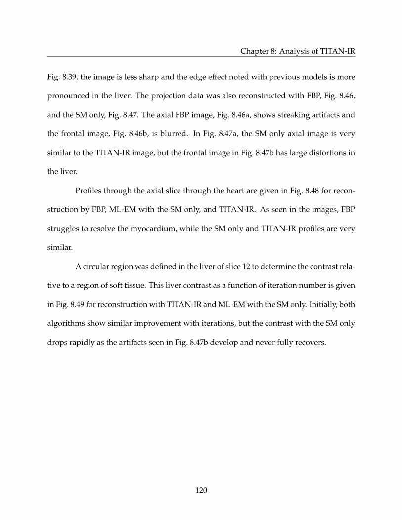
Chapter 8: Analysis of TITAN-IR
Fig. 8.39, the image is less sharp and the edge effect noted with previous models is more
pronounced in the liver. The projection data was also reconstructed with FBP, Fig. 8.46,
and the SM only, Fig. 8.47. The axial FBP image, Fig. 8.46a, shows streaking artifacts and
the frontal image, Fig. 8.46b, is blurred. In Fig. 8.47a, the SM only axial image is very
similar to the TITAN-IR image, but the frontal image in Fig. 8.47b has large distortions in
the liver.
Profiles through the axial slice through the heart are given in Fig. 8.48 for recon-
struction by FBP, ML-EM with the SM only, and TITAN-IR. As seen in the images, FBP
struggles to resolve the myocardium, while the SM only and TITAN-IR profiles are very
similar.
A circular region was defined in the liver of slice 12 to determine the contrast rela-
tive to a region of soft tissue. This liver contrast as a function of iteration number is given
in Fig. 8.49 for reconstruction with TITAN-IR and ML-EM with the SM only. Initially, both
algorithms show similar improvement with iterations, but the contrast with the SM only
drops rapidly as the artifacts seen in Fig. 8.47b develop and never fully recovers.
120
Chapter 8: Analysis of TITAN-IR
(a) Axial slice 16 (b) Frontal slice 18
Figure 8.45: TITAN-IR (S8, base meshing) reconstructed images from noisy GE-LEGPprojection data after 40 iterations
(a) Axial slice 16 (b) Frontal slice 18
Figure 8.46: FBP reconstructed images from noisy GE-LEGP projection data
(a) Axial slice 16 (b) Frontal slice 18
Figure 8.47: SM only reconstructed images from noisy GE-LEGP projection data after40 iterations
121
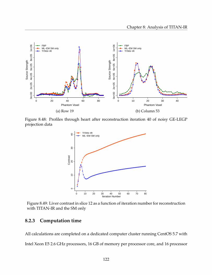
Chapter 8: Analysis of TITAN-IR
0 20 40 60 80
0e+
002e
+05
4e+
056e
+05
8e+
051e
+06
Phantom Voxel
Sou
rce
Str
engt
h
Noisy GE−LEGP Data Row 19 40 iterations
FBPML−EM SM onlyTITAN−IR
(a) Row 19
0 10 20 30 40
0e+
002e
+05
4e+
056e
+05
8e+
051e
+06
Phantom Voxel
Sou
rce
Str
engt
h
FBPML−EM SM onlyTITAN−IR
(b) Column 53
Figure 8.48: Profiles through heart after reconstruction iteration 40 of noisy GE-LEGPprojection data
0 10 20 30 40 50 60 70 80
010
2030
40
Iteration Number
Con
tras
t
TITAN−IRML−EM SM only
Figure 8.49: Liver contrast in slice 12 as a function of iteration number for reconstructionwith TITAN-IR and the SM only
8.2.3 Computation time
All calculations are completed on a dedicated computer cluster running CentOS 5.7 with
Intel Xeon E5 2.6 GHz processors, 16 GB of memory per processor core, and 16 processor
122

Chapter 8: Analysis of TITAN-IR
cores per compute node. For the following computation times, the deterministic simula-
tion uses S8 quadrature and base meshing.
The computation time for a standard ML-EM reconstruction of the NCAT phan-
tom by TITAN-IR of noiseless data with no collimator blur on 16 processor cores is 42.0 s
for 40 iterations. Of those 42.0 s, 2.8 s are spent loading inputs and initializing the re-
construction. The OS-EM reconstruction times for varying numbers of subsets are given
in Table 8.20. Note that the total number of sub-iterations in Table 8.20 remains 40 for
all cases, e.g., 10 full iterations with 4 subsets is equivalent to 40 ML-EM iterations. The
reduction in computation time with increasing subsets is only 2 to 3 seconds. With the
fine meshing deterministic model, the ML-EM computation time becomes 305 s for 40
iterations.
Table 8.20: Computation time for 40 iterationsof TITAN-IR (S8, base meshing) on noiselessprojection data with no collimator blur
Angles per TimeSubsets subset (s) Speedup
1 64 42.0 -2 32 39.8 1.064 16 39.1 1.078 8 38.9 1.08
Table 8.21: Computation time for 40 iter-ations of TITAN-IR (S8, base meshing) onnoisy GE-LEGP projection data
Angles per TimeSubsets subset (s) Speedup
1 64 218.8 -2 32 204.2 1.074 16 194.4 1.138 8 195.4 1.12
For reconstruction of GE-LEGP projection data, the sparse system matrix is now
over 9 GB instead of the 177 MB required for the projection data with no collimator blur
and reading in inputs and initializing the reconstruction takes 143.3 s. Regardless of it-
erative reconstruction method, reducing the system matrix size can significantly reduce
123

Chapter 8: Analysis of TITAN-IR
computation time. The computation time for different numbers of subsets for 40 iterations
over-all is given in Table 8.21. The OS-EM algorithm reduces the ML-EM reconstruction
time by 24 s or 11%. A larger speedup is seen if the number of iterations is increased.
124
Chapter 9
Conclusions and Future Work
The TITAN code’s ability to generate SPECT projection images has been benchmarked
through comparison with results from the SIMIND and MCNP5 Monte Carlo codes as
well as an experiment. The TITAN projection images were shown to match well with
other methods, in particular for small collimator acceptance angles, and the TITAN code
was consistently shown to have the superior computation time. A modified algorithm
for representing the collimator called weighted circular ordinate splitting (WCOS) was
developed and tested. The parallel behavior of the TITAN SPECT simulation has been
studied and improved upon.
The DRS methodology, which reconstructs SPECT projection images using a de-
terministic transport code, has been developed and tested for ML-EM iterative image
reconstruction. The methodology uses a deterministic transport code to fully model the
particle transport in a patient during the forward projection step of ML-EM without the
125
Chapter 9: Conclusions and Future Work
generation of the large system matrix that would be needed to model scatter. DRS was
implemented into a script that could be used by anyone with a transport code that cre-
ates projection data. The script was tested with a 2-dimensional elliptical water phantom
with excellent results; however, computation times are lengthened due to the need to
repeatedly read and write files with an external script.
Using the DRS methodology, the TITAN deterministic transport code has been
modified for image reconstruction to create the TITAN-IR code. The TITAN-IR code per-
forms ML-EM or OS-EM reconstruction from SPECT projection data in parallel. The user
must supply the projection data to reconstruct and a system matrix for backprojection. In
addition to iterative image reconstruction, a variety of quality metrics are incorporated
into TITAN-IR, including the log-likelihood, relative errors between generated projec-
tions and measured data, background noise, and contrast.
TITAN-IR has been used to successfully reconstruct a Jaszczak cold sphere phan-
tom and NCAT phantom from projection data generated using the SIMIND Monte Carlo
code. Extensive parameter studies on the Jaszczak phantom examined the dependency
of reconstruction quality on deterministic parameters, e.g., quadrature order, mesh size,
anisotropic scattering order, and differencing scheme. It was discovered that for these
models the reconstruction images are largely insensitive to parameter selection. Deter-
ministic methods tend to be sensitive to parameter selection, so this finding is important
to the utility of TITAN-IR.
126
Chapter 9: Conclusions and Future Work
The ability of TITAN-IR to reconstruct projection data with different degrees of
noise and collimator blur was examined in detail with the Jaszczak phantom. The new
code demonstrated stable and predictable behavior while handling the addition of these
complications. The projection data was also reconstructed using FBP with the Chang
attenuation correction and ML-EM with the SM only, i.e., without scatter modeled. With
the addition of noise and collimator blur to the Jaszczak phantom projection data, the
advantages of TITAN-IR modeling scatter were no longer apparent for this particular
case compared with the SM only images. However, the cold sphere contrast had far more
stable convergence in TITAN-IR images than the SM only images. The NCAT phantom
introduced reconstruction with a heterogeneous phantom and more complicated source
distribution. TITAN-IR was able to reconstruct the strong source in both the myocardium
and liver, while the SM only images showed severe artifacts in the liver.
Computation time is an important factor in the feasibility of TITAN-IR for ap-
plication in both a research and a clinical setting. In a deterministic transport code, pa-
rameter selection largely drives computation time and so showing a lack of sensitivity of
the reconstruction to parameter selection allowed for time to be minimized. The Jaszczak
phantom projection data with no collimator blur took 37 s to complete 64 iterations on 16
processor cores with ML-EM. This computation time increased to 172 s for the GE-LEGP
projection data, in large part due to the significantly larger system matrix associated with
including collimator blur. Using OS-EM with 4 subsets reduced this computation time to
140 s. The same behavior was observed with the NCAT phantom.
127
Chapter 9: Conclusions and Future Work
The results of this work have indicated that deterministic reconstruction of
SPECT data is feasible and opened the door to a wide variety of additional research.
Some of these that are particularly interesting to the researcher are the following.
Reconstruction of clinical data
At this point, TITAN-IR has only been used to reconstruct simulated projection data. Col-
laboration is underway with The Penn State Hershey Cancer Center with the assistance of
Michele Ferenci, Chief of Medical Physics, and Karen Brown, Associate Health Physicist,
to use TITAN-IR to reconstruct data from a SPECT device. The Hershey Cancer Center is
providing projection data acquired from a Jaszczak Phantom with their Siemens Symbia
SPECT system as part of their quality assurance program. Reconstruction of data ac-
quired on a clinical SPECT device will be an important step in the validation of TITAN-IR
and hopefully be followed by the reconstruction of patient data.
Multi-energy reconstruction
It would be interesting to apply TITAN-IR to cases in which either the radionuclide in the
patient emits photons at different energies or multiple radionuclides are present. Down-
scatter from higher energy photons to the lower energy photopeak(s) is the primary issue
with this type of imaging. Since TITAN already solves the multigroup transport equation,
no modification would be needed to the base TITAN code to model multiple photon en-
ergies and the down-scatter between them. This is a logical and very promising extension
of the capabilities of the TITAN-IR code.
128
Chapter 9: Conclusions and Future Work
Along the same lines, it may be possible in cases of single-energy emissions to use
lower energy groups as part of the reconstruction since TITAN-IR can accurately model
the scattering of emitted photons to lower energies. Hutton et al. suggested that with
accurate modeling of scatter a wider range of energies could be included43. Including
more counts in the reconstruction could lead to reduced doses and acquisition times,
provided those additional counts are modeled properly.
Additional possibilities
The DRS methodology could readily be applied to other iterative reconstruction algo-
rithms besides ML-EM as well as other deterministic codes. In particular, it would im-
prove the utility of TITAN-IR to provide users with a variety of reconstruction algorithms
to choose from. Several performance metrics are already calculated in TITAN-IR to facil-
itate determination of convergence, but this capability should be expanded to improve
understanding and give the user more guidance. It would also be interesting to investi-
gate the use of an adjoint methodology with TITAN75 to calculated the system matrix.
129
Bibliography
[1] S. R. Cherry, J. A. Sorenson, and M. E. Phelps, Physics in Nuclear Medicine, 3rd ed.,A. Ross, Ed. Saunders, 2003.
[2] IMV Medical Information Division, Inc., “2011 nuclear medicine market outlook re-port.”
[3] J. T. Bushberg, J. A. Seibert, J. Edwin M. Leidholdt, and J. M. Boone, The EssentialPhysics of Medical Imaging. Lippincott Williams & Wilkins, 2002.
[4] C. Yi, “Hybrid discrete ordinates and characteristics method for solving linear Boltz-mann equation,” Ph.D. dissertation, University of Florida, 2007.
[5] G. Hevesy, “The absorption and translocation of lead by plants: A contribution to theapplication of the method of radioactive indicators in the investigation of the changeof substance in plants,” Biochem J., vol. 17, pp. 439–445, 1923.
[6] E. O. Lawrence and M. S. Livingston, “The production of high speed light ionswithout the use of high voltages,” Phys. Rev., vol. 40, pp. 19–35, April 1932.
[7] H. O. Anger, “Scintillation camera,” Rev. Sci. Instrum., vol. 29, no. 1, pp. 27–33, 1958.
[8] P. Harper, R. Beck, D. Charleston, and K. Lathrop, “Optimization of a scanningmethod using Tc-99m,” Nucleonics, vol. 22, pp. 50–54, 1964.
[9] W. Tucker, M. Greene, A. Weiss, and A. Murrenhoff, “Methods of preparation ofsome carrier-free radioisotopes involving sorption on alumina,” Brookhaven Na-tional Laboratory, BNL 3746, Tech. Rep., 1958.
[10] D. E. Kuhl and R. Q. Edwards, “Cylindrical and section radioisotope scanning of theliver and brain,” Radiology, vol. 83, pp. 926–936, 1964.
[11] H. O. Anger, ”Tomographic gamma-ray scanner with simultaneous read-out of sev-eral planes” in Fundamental Problems of Scanning. Springfield, IL: Charles C. Thomas,1968, pp. 195–211.
130
Bibliography
[12] R. Jaszczak, P. Murphy, D. Huard, and J. Burdine, “Radionuclide emission computedtomography of the head with 99mTc and a scintillation camera,” J Nucl Med, vol. 18,no. 4, pp. 373–380, 1977.
[13] J. Keyes, N. Orlandea, W. Heetderks, P. Leonard, and W. Rogers, “The humongotron:a scintillation-camera transaxial tomograph,” J Nucl Med, vol. 18, pp. 381–387, 1977.
[14] M. Bocher, A. Balan, Y. Krausz, Y. Shrem, A. Lonn, M. Wilk, and R. Chisin, “Gammacamera-mounted anatomical x-ray tomography: technology, system characteristicsand first images,” European Journal of Nuclear Medicine, vol. 27, pp. 619–627, 2000.
[15] M. K. O’Connor and B. J. Kemp, “Single-photon emission computed tomogra-phy/computed tomography: Basic instrumentation and innovations,” Seminars inNuclear Medicine, vol. 36, no. 4, pp. 258–266, 2006.
[16] M. T. Madsen, “Recent advances in SPECT imaging,” Journal of Nuclear Medicine,vol. 48, pp. 661–673, 2007.
[17] J. Radon, “Uber die bestimmung von funktionen durch ihre integralwerte langsgewisser mannigfaltigkeiten,” Berichte Sachsische Akadamie der Wissenschaften, Leipzig,Math. Phys. Kl., vol. 69, pp. 262–277, 1917.
[18] P. P. Bruyant, “Analytic and iterative reconstruction algorithms in SPECT,” Journal ofNuclear Medicine, vol. 43, pp. 1343–1358, 2002.
[19] A. M. Cormack, “Representation of a function by its line integrals, with someradiological applications,” Journal of Applied Physics, vol. 34, no. 9, pp. 2722–2727,1963.
[20] D. E. Kuhl and R. Q. Edwards, “Image separation radioisotope scanning,” Radiology,vol. 80, pp. 653–662, 1963.
[21] R. Gordon, R. Bender, and G. Herman, “Algebraic reconstruction techniques(ART) for three-dimensional electron microscopy and x-ray photography.” Journal ofTheoretical Biology, vol. 29, no. 3, pp. 471–481, Dec. 1970.
[22] P. Gilbert, “Iterative methods for the three-dimensional reconstruction of an objectfrom projections,” Journal of Theoretical Biology, vol. 36, no. 1, pp. 105–117, 1972.
[23] L. A. Shepp and Y. Vardi, “Maximum likelihood reconstruction for emission tomog-raphy,” IEEE Transactions on Medical Imaging, vol. 1, no. 2, pp. 113–122, Oct. 1982.
[24] K. Lange and R. Carson, “EM reconstruction algorithms for emission andtransmission tomography.” J Comput Assist Tomogr, vol. 8, pp. 306–316, 1984.
131
Bibliography
[25] H. Hudson and R. Larkin, “Accelerated image reconstruction using ordered subsetsof projection data,” IEEE Transactions on Medical Imaging, vol. 13, no. 4, pp. 601–609,Dec. 1994.
[26] B. F. Hutton, “Recent advances in iterative reconstruction for clinical SPECT/PETand CT,” Acta Oncologica, vol. 50, no. 6, pp. 851–858, 2011.
[27] S. Vandenberghe, Y. D’Asseler, R. V. de Walle, T. Kauppinen, M. Koole, L. Bouwens,K. V. Laere, I. Lemahieu, and R. Dierckx, “Iterative reconstruction algorithms innuclear medicine,” Computerized Medical Imaging and Graphics, vol. 25, no. 2, pp.105–111, 2001.
[28] S. Staelens, D. Strul, G. Santin, S. Vandenberghe, M. Koole, Y. D’Asseler, I. Lemahieu,and R. V. de Walle, “Monte carlo simulations of a scintillation camera using GATE:validation and application modelling,” Physics in Medicine and Biology, vol. 48,no. 18, pp. 3021–42, 2003.
[29] J. C. Yanch, A. B. Dobrzeniecki, C. Ramanathan, and R. Behrman, “Physicallyrealistic monte carlo simulation of source, collimator and tomographic dataacquisition for emission computed tomography,” Physics in Medicine and Biology,vol. 37, no. 4, pp. 853–870, 1992.
[30] R. Harrison, D. Haynor, S. Gillispie, and S. Vannoy, “A public-domain simulationsystem for emission tomography - photon tracking through heterogeneous attenua-tion using importance sampling,” The Journal of Nuclear Medicine, vol. 34, no. 5, May1993.
[31] M. Ljungberg and S.-E. Strand, “A Monte Carlo program for the simulation ofscintillation camera characteristics,” Computer Methods and Programs in Biomedicine,vol. 29, no. 4, pp. 257–272, 1989.
[32] S. Agostinelli, “Geant4-a simulation toolkit,” Nuclear Instruments and Methodsin Physics Research Section A: Accelerators, Spectrometers, Detectors and AssociatedEquipment, vol. 506, no. 3, pp. 250–303, 2003.
[33] F. Brown, R. Barrett, T. Booth, J. Bull, L. Cox, R. Forster, T. Goorley, R. Mosteller,S. Post, R. Prael, E. Selcow, A. Sood, and J. Sweezy, “MCNP Version 5,” Trans. Am.Nucl. Soc., vol. 87, pp. 273–276, 2002.
[34] T. A. Riauka and Z. W. Gortel, “Photon propagation and detection in single-photonemission computed tomography-an analytical approach,” Med. Phys., vol. 21, no. 8,pp. 1311–1321, August 1994.
[35] R. Wells, A. Celler, and R. Harrop, “Analytical calculation of photon distributionsin SPECT projections,” IEEE Transactions on Nuclear Science, vol. 45, no. 6, pp. 3202–3214, 1998.
132
Bibliography
[36] J. Fessler, “Iterative methods for image reconstruction,” 2008. [Online]. Available:http://www.eecs.umich.edu/∼fessler/papers/files/talk/08/isbi-notes.pdf
[37] G. K. Loudos, P. Papadimitroulas, P. Zotos, I. Tsougos, and P. Georgoulias, “Develop-ment and evaluation of QSPECT open-source software for the iterative reconstruc-tion of SPECT images.” Nuclear Medicine Communications, vol. 31, no. 6, pp. 558–566,2010.
[38] K. Thielemans, C. Tsoumpas, S. Mustafovic, T. Beisel, P. Aguiar, N. Dikaios, , andM. W. Jacobson, “STIR: Software for tomographic image reconstruction release 2,”Physics in Medicine and Biology, vol. 57, no. 4, pp. 867–883, 2012.
[39] B. M. Fuster, C. Falcon, C. Tsoumpas, L. Livieratos, P. Aguiar, A. Cot, D. Ros, andK. Thielemans, “Integration of advanced 3D SPECT modeling into the open-sourceSTIR framework,” Medical Physics, vol. 40, no. 9, 2013.
[40] S. Pedemonte, A. Bousse, K. Erlandsson, M. Modat, S. Arridge, B. F. Hutton, andS. Ourselin, “GPU accelerated rotation-based emission tomography reconstruction,”in Proc. IEEE MIC 2010, Knoxville, TN, Oct. 30-Nov. 6 2010.
[41] A. Hara, R. Paden, A. Silva, J. Kujak, H. Lawder, and W. Pavlicek, “Iterative re-construction technique for reducing body radiation dose at CT: Feasibility study,”American Journal of Roentgenology, vol. 193, no. 3, pp. 764–771, 2009.
[42] P. Green, “Bayesian reconstructions from emission tomography data using a mod-ified EM algorithm,” IEEE Transactions on Medical Imaging, vol. 9, no. 1, pp. 84–93,1990.
[43] B. F. Hutton, I. Buvat, and F. J. Beekman, “Review and current status of SPECTscatter corrections,” Physics in Medicine and Biology, vol. 56, no. 14, 2011.
[44] C. Kamphuis, F. J. Beekman, P. P. van Rijk, and M. A. Viergever, “Dual matrixordered subsets reconstruction for accelerated 3D scatter compensation in single-photon emission tomography,” European Journal of Nuclear Medicine and MolecularImaging, vol. 25, pp. 8–18, 1998.
[45] E. Frey, K. Gilland, and B. Tsui, “Application of task-based measures of image qual-ity to optimization and evaluation of three-dimensional reconstruction-based com-pensation methods in myocardial perfusion SPECT,” IEEE Transactions on MedicalImaging, vol. 21, no. 9, pp. 1040–1050, 2002.
[46] J. Xiao, F. Verzijlbergen, M. Viergever, and F. Beekman, “Small field-of-viewdedicated cardiac SPECT systems: impact of projection truncation,” European Journalof Nuclear Medicine and Molecular Imaging, vol. 37, pp. 528–536, 2010.
133
Bibliography
[47] E. C. Frey and B. Tsui, “A new method for modeling the spatially-variant, object-dependent scatter response function in SPECT,” in Nuclear Science Symposium, 1996Conference Record, vol. 2, 1996, pp. 1082–1086.
[48] F. Beekman, H. de Jong, and S. van Geloven, “Efficient fully 3-D iterative SPECTreconstruction with monte carlo-based scatter compensation,” IEEE Transactions onMedical Imaging, vol. 21, no. 8, pp. 867–877, 2002.
[49] F. J. Beekman, H. W. de Jong, and E. T. Slijpen, “Efficient SPECT scatter calculationin non-uniform media using correlated monte carlo simulation,” Physics in Medicineand Biology, vol. 44, no. 8, pp. N183–92, 1999.
[50] G. Zeng and G. Gullberg, “Unmatched projector/backprojector pairs in an iterativereconstruction algorithm,” IEEE Transactions on Medical Imaging, vol. 19, no. 5, pp.548–555, May 2000.
[51] J. J. Duderstadt and L. J. Hamilton, Nuclear Reactor Analysis. John Wiley and Sons,1976.
[52] E. E. Lewis and W. F. Miller, Computational Methods of Neutron Transport. John Wileyand Sons, 1984.
[53] B. G. Petrovic and A. Haghighat, “Analysis of inherent oscillations in multidimen-sional solutions of the neutron transport equation,” Nuclear Science and Engineering,vol. 124, pp. 31–62, 1996.
[54] C. Yi and A. Haghighat, “A three-dimensional block-oriented hybrid discrete ordi-nates and characteristics method,” Nuclear Science and Engineering, vol. 164, no. 3, pp.221–247, 2010.
[55] G. I. Bell and S. Glasstone, Nuclear Reactor Theory. Malabar, FL: Robert E. KreigerPublishing, 1985.
[56] B. Petrovic and A. Haghighat, “New directional theta-weighted Sn differencingscheme and its application to pressure vessel fluence calculations,” Proc. RadiationProtection and Shielding Topical Meeting, vol. I, pp. 3–10, 1996.
[57] C. Yi and A. Haghighat, “Hybrid SN and ray-tracing with fictitious quadrature forsimulation of SPECT,” in Proc. M&C 2009. Saratoga Springs, New York: AmericanNuclear Society, May 3-7 2009, [CD-ROM].
[58] G. Longoni and A. Haghighat, “Development of the regional angular refinement andits application to the CT-scan device,” Transactions of the American Nuclear Society,vol. 86, pp. 246–248, 2002.
134
Bibliography
[59] L. J. Lorence, J. E. Morel, and G. D. Valdez, User’s Guide to CEPXS/ONELD: A One-Dimensional Coupled Electron-Photon Discrete Ordinates Code Package Version 1.0, San-dia National Laboratory, SAND89-1161, 1989.
[60] K. Royston, A. Haghighat, C. Yi, A. Cebula, and D. Gilland, “Validation of a new de-terministic transport code for SPECT simulation,” in Proc. IEEE MIC 2010, Knoxville,TN, Oct. 30-Nov. 6 2010, [CD-ROM].
[61] W. P. Segars, “Development and application of the new dynamic NURBS-basedcardiac-torso (NCAT) phantom,” Ph.D. dissertation, University of North Carolina,2001.
[62] K. Royston, A. Haghighat, and C. Yi, “Comparison of TITAN hybrid deterministictransport code and MCNP5 for simulation of SPECT,” Progress in Nuclear Science andTechnology, vol. 2, pp. 201–206, 2011.
[63] M. Studenski, D. Gilland, J. Parker, B. Hammond, S. Majewski, A. Weisenberger,and V. Popov, “Performance evaluation of a bedside cardiac SPECT system,” IEEETransactions on Nuclear Science, vol. 56, no. 3, pp. 625–632, 2009.
[64] K. K. Royston and A. Haghighat, “Sensitivity analysis of the TITAN hybrid deter-ministic transport code for SPECT simulation,” in Proc. M&C 2011. Rio de Janeiro,RJ, Brazil: Latin American Section/American Nuclear Society, May 8-12 2011, [CD-ROM].
[65] G. M. Amdahl, “Validity of the single processor approach to achieving large scalecomputing capabilities,” in Proceedings of AFIPS, April 18-20, 1967, vol. 30, NewYork, NY, USA, 1967, pp. 483–485.
[66] K. Royston, A. Haghighat, and C. Yi, “Application of TITAN for simulation of par-ticle streaming in a duct,” in Proc. 15th ISRD, Aix en Provence, France, May 18-232014.
[67] K. Royston and A. Haghighat, “Development of a collimator representation in theTITAN transport code for SPECT simulation,” in Proc. IEEE MIC 2012, Anaheim,CA, Oct. 29-Nov. 3 2012, [CD-ROM].
[68] K. Royston and A. Haghighat, “Performance of the new WCOS technique for theTITAN SPECT formulation,” in Proc. SNA+MC 2013, Paris, France, Oct. 27-31 2013.
[69] B. Petrovic and A. Haghighat, “New directional theta-weighted (DTW) differenc-ing scheme and reduction of estimated pressure vessel fluence uncertainty,” Prague,Czech Republic, September 2-6 1996.
[70] D. L. Snyder, M. I. Miller, L. J. Thomas, and D. G. Politte, “Noise and edge artifactsin mazimum-likelihood reconstructions for emission tomography,” IEEE Transactionson Medical Imaging, vol. MI-6, no. 3, pp. 228–238, 1987.
135

Bibliography
[71] M. Frigo and S. G. Johnson, “The design and implementation of FFTW3,” Proc. ofIEEE, vol. 93, no. 2, pp. 216–231, 2005.
[72] L. S. Graham, F. H. Fahey, M. T. Madsen, A. van Aswegen, and M. V. Yester, “Quanti-tation of SPECT performance: report of task group 4, nuclear medicine committee,”Medical Physics, vol. 22, no. 4, pp. 401–409, 1995.
[73] C. E. Metz, F. B. Atkins, and R. N. Beck, “The geometric transfer function componentfor scintillation camera collimators with straight parallel holes,” Physics in Medicineand Biology, vol. 25, no. 6, 1980.
[74] L.-T. Chang, “A method for attenuation correction in radionuclide computed tomog-raphy,” IEEE Transactions on Nuclear Science, vol. 25, no. 1, pp. 638–643, 1978.
[75] K. Royston, A. Haghighat, and C. Yi, “Verification of a hybrid adjoint methodologyin TITAN for single photon emission computed tomography,” in Proc. PHYSOR 2010,Pittsburgh, PA, May 9-14 2010, [CD-ROM].
136

Appendices
137
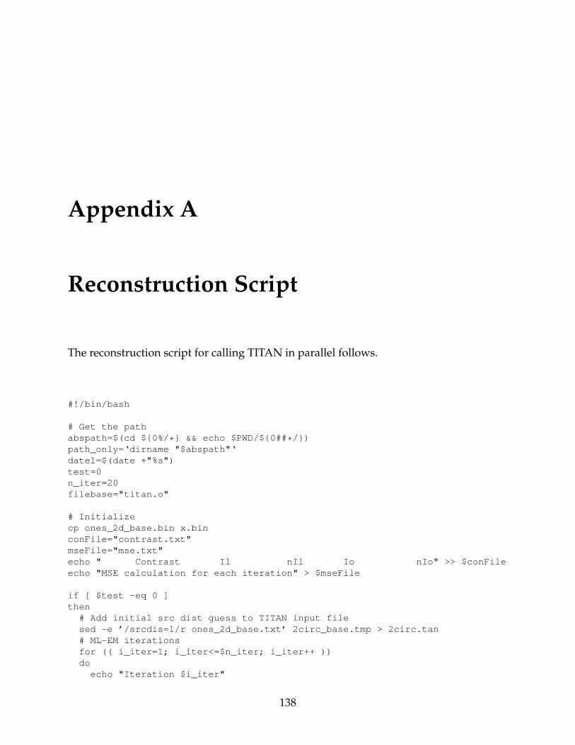
Appendix A
Reconstruction Script
The reconstruction script for calling TITAN in parallel follows.
#!/bin/bash
# Get the pathabspath=$(cd $0%/* && echo $PWD/$0##*/)path_only=‘dirname "$abspath"‘date1=$(date +"%s")test=0n_iter=20filebase="titan.o"
# Initializecp ones_2d_base.bin x.binconFile="contrast.txt"mseFile="mse.txt"echo " Contrast Il nIl Io nIo" >> $conFileecho "MSE calculation for each iteration" > $mseFile
if [ $test -eq 0 ]then
# Add initial src dist guess to TITAN input filesed -e ’/srcdis=1/r ones_2d_base.txt’ 2circ_base.tmp > 2circ.tan# ML-EM iterationsfor (( i_iter=1; i_iter<=$n_iter; i_iter++ ))do
echo "Iteration $i_iter"
138
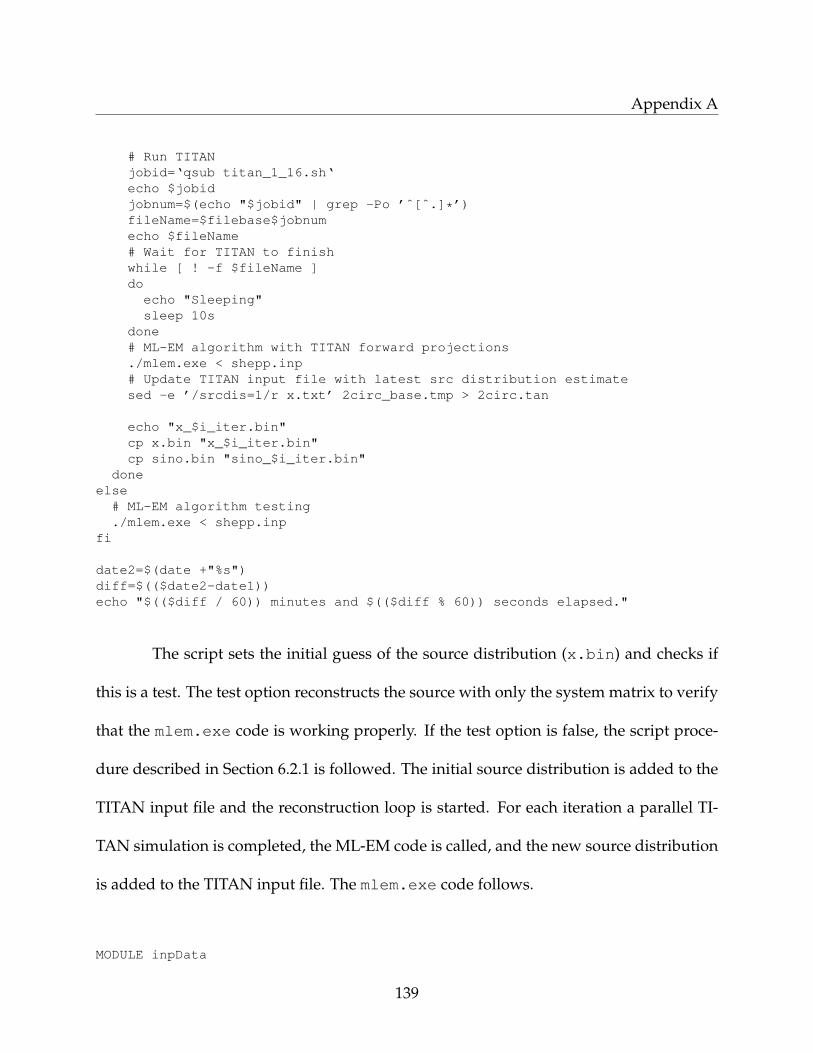
Appendix A
# Run TITANjobid=‘qsub titan_1_16.sh‘echo $jobidjobnum=$(echo "$jobid" | grep -Po ’ˆ[ˆ.]*’)fileName=$filebase$jobnumecho $fileName# Wait for TITAN to finishwhile [ ! -f $fileName ]do
echo "Sleeping"sleep 10s
done# ML-EM algorithm with TITAN forward projections./mlem.exe < shepp.inp# Update TITAN input file with latest src distribution estimatesed -e ’/srcdis=1/r x.txt’ 2circ_base.tmp > 2circ.tan
echo "x_$i_iter.bin"cp x.bin "x_$i_iter.bin"cp sino.bin "sino_$i_iter.bin"
doneelse
# ML-EM algorithm testing./mlem.exe < shepp.inp
fi
date2=$(date +"%s")diff=$(($date2-date1))echo "$(($diff / 60)) minutes and $(($diff % 60)) seconds elapsed."
The script sets the initial guess of the source distribution (x.bin) and checks if
this is a test. The test option reconstructs the source with only the system matrix to verify
that the mlem.exe code is working properly. If the test option is false, the script proce-
dure described in Section 6.2.1 is followed. The initial source distribution is added to the
TITAN input file and the reconstruction loop is started. For each iteration a parallel TI-
TAN simulation is completed, the ML-EM code is called, and the new source distribution
is added to the TITAN input file. The mlem.exe code follows.
MODULE inpData
139
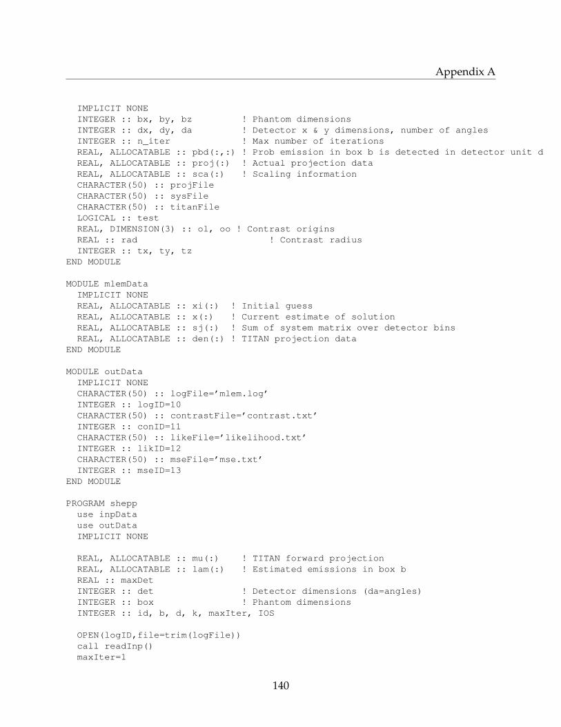
Appendix A
IMPLICIT NONEINTEGER :: bx, by, bz ! Phantom dimensionsINTEGER :: dx, dy, da ! Detector x & y dimensions, number of anglesINTEGER :: n_iter ! Max number of iterationsREAL, ALLOCATABLE :: pbd(:,:) ! Prob emission in box b is detected in detector unit dREAL, ALLOCATABLE :: proj(:) ! Actual projection dataREAL, ALLOCATABLE :: sca(:) ! Scaling informationCHARACTER(50) :: projFileCHARACTER(50) :: sysFileCHARACTER(50) :: titanFileLOGICAL :: testREAL, DIMENSION(3) :: ol, oo ! Contrast originsREAL :: rad ! Contrast radiusINTEGER :: tx, ty, tz
END MODULE
MODULE mlemDataIMPLICIT NONEREAL, ALLOCATABLE :: xi(:) ! Initial guessREAL, ALLOCATABLE :: x(:) ! Current estimate of solutionREAL, ALLOCATABLE :: sj(:) ! Sum of system matrix over detector binsREAL, ALLOCATABLE :: den(:) ! TITAN projection data
END MODULE
MODULE outDataIMPLICIT NONECHARACTER(50) :: logFile=’mlem.log’INTEGER :: logID=10CHARACTER(50) :: contrastFile=’contrast.txt’INTEGER :: conID=11CHARACTER(50) :: likeFile=’likelihood.txt’INTEGER :: likID=12CHARACTER(50) :: mseFile=’mse.txt’INTEGER :: mseID=13
END MODULE
PROGRAM sheppuse inpDatause outDataIMPLICIT NONE
REAL, ALLOCATABLE :: mu(:) ! TITAN forward projectionREAL, ALLOCATABLE :: lam(:) ! Estimated emissions in box bREAL :: maxDetINTEGER :: det ! Detector dimensions (da=angles)INTEGER :: box ! Phantom dimensionsINTEGER :: id, b, d, k, maxIter, IOS
OPEN(logID,file=trim(logFile))call readInp()maxIter=1
140
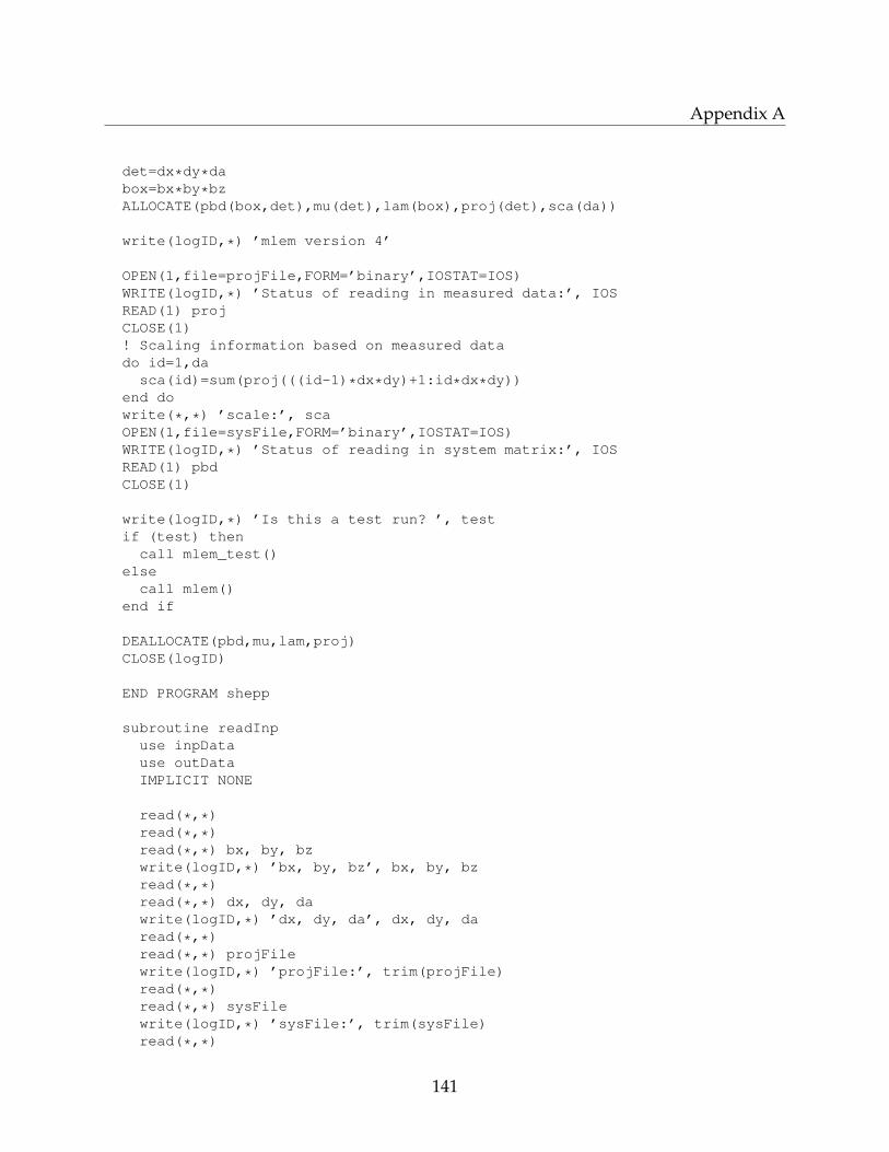
Appendix A
det=dx*dy*dabox=bx*by*bzALLOCATE(pbd(box,det),mu(det),lam(box),proj(det),sca(da))
write(logID,*) ’mlem version 4’
OPEN(1,file=projFile,FORM=’binary’,IOSTAT=IOS)WRITE(logID,*) ’Status of reading in measured data:’, IOSREAD(1) projCLOSE(1)! Scaling information based on measured datado id=1,da
sca(id)=sum(proj(((id-1)*dx*dy)+1:id*dx*dy))end dowrite(*,*) ’scale:’, scaOPEN(1,file=sysFile,FORM=’binary’,IOSTAT=IOS)WRITE(logID,*) ’Status of reading in system matrix:’, IOSREAD(1) pbdCLOSE(1)
write(logID,*) ’Is this a test run? ’, testif (test) then
call mlem_test()else
call mlem()end if
DEALLOCATE(pbd,mu,lam,proj)CLOSE(logID)
END PROGRAM shepp
subroutine readInpuse inpDatause outDataIMPLICIT NONE
read(*,*)read(*,*)read(*,*) bx, by, bzwrite(logID,*) ’bx, by, bz’, bx, by, bzread(*,*)read(*,*) dx, dy, dawrite(logID,*) ’dx, dy, da’, dx, dy, daread(*,*)read(*,*) projFilewrite(logID,*) ’projFile:’, trim(projFile)read(*,*)read(*,*) sysFilewrite(logID,*) ’sysFile:’, trim(sysFile)read(*,*)
141

Appendix A
read(*,*) n_iterread(*,*)read(*,*) titanFilewrite(logID,*) ’titanFile:’, trim(titanFile)read(*,*)read(*,*) testread(*,*)read(*,*) ol(1), ol(2), ol(3), oo(1), oo(2), oo(3), radwrite(logID,*) ’Contrast parameters:’, ol(:), oo(:), radread(*,*)read(*,*) tx, ty, tz
end subroutine readInp
subroutine mlemuse inpDatause mlemDatause outDataIMPLICIT NONE
logical :: isnanf, isinffINTEGER :: ib, id, ia, idx, idyINTEGER :: box, detINTEGER :: i_iter, IOSREAL :: dsum, maxTmp
box=bx*by*bzdet=dx*dy*daallocate(xi(box),x(box),sj(box))allocate(den(det))
OPEN(1,file=’x.bin’,form=’binary’,IOSTAT=IOS)READ(1) xiCLOSE(1)den(:)=0.0sj(:)=0.0do ib=1,box
sj(ib)=sum(pbd(ib,:))end do
i_iter=0i_iter=i_iter+1
OPEN(2,file=trim(titanFile),form=’binary’,iostat=IOS)WRITE(logID,*) ’Read TITAN sinogram status:’, IOSdo ia=1,da
do id=1,dx*dyREAD(2) den(det-(ia*dx*dy)+id)
end doend doCLOSE(2)
! Scale TITAN sinogram to match projection data
142
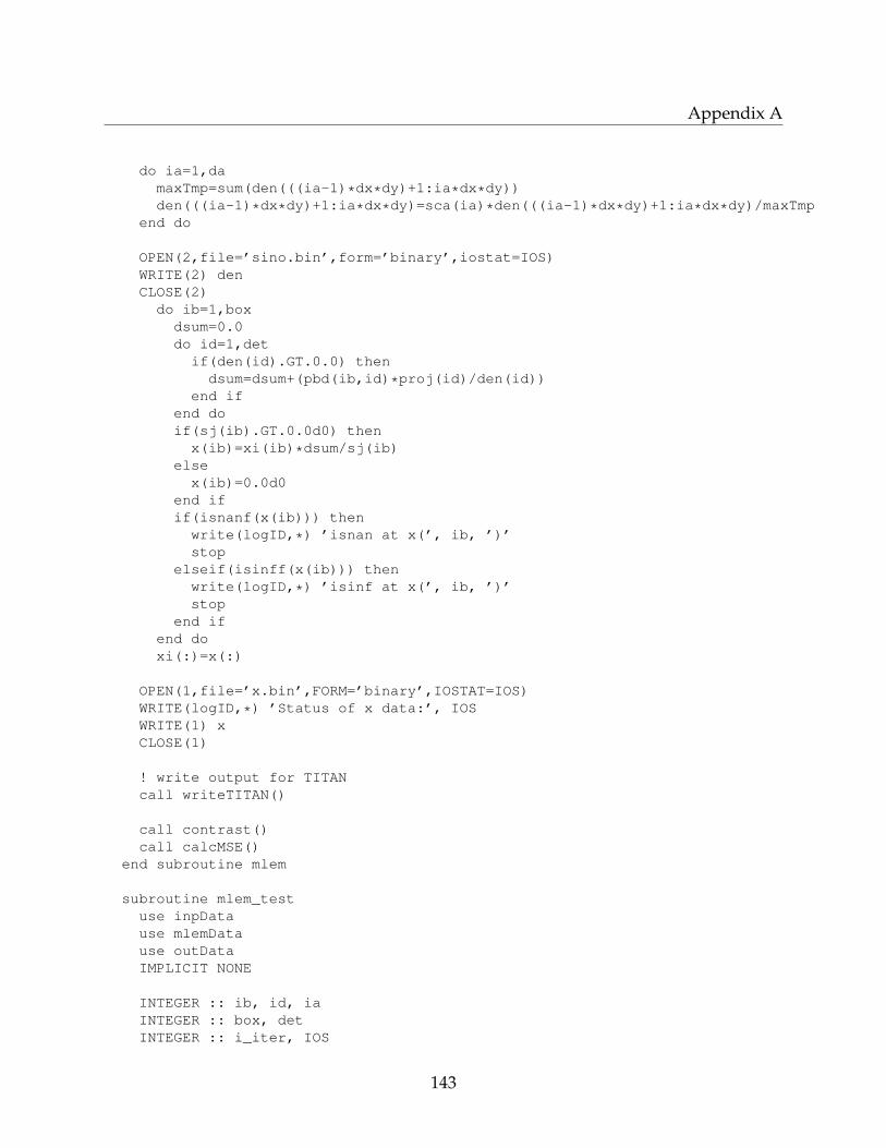
Appendix A
do ia=1,damaxTmp=sum(den(((ia-1)*dx*dy)+1:ia*dx*dy))den(((ia-1)*dx*dy)+1:ia*dx*dy)=sca(ia)*den(((ia-1)*dx*dy)+1:ia*dx*dy)/maxTmp
end do
OPEN(2,file=’sino.bin’,form=’binary’,iostat=IOS)WRITE(2) denCLOSE(2)
do ib=1,boxdsum=0.0do id=1,detif(den(id).GT.0.0) then
dsum=dsum+(pbd(ib,id)*proj(id)/den(id))end if
end doif(sj(ib).GT.0.0d0) then
x(ib)=xi(ib)*dsum/sj(ib)else
x(ib)=0.0d0end ifif(isnanf(x(ib))) then
write(logID,*) ’isnan at x(’, ib, ’)’stop
elseif(isinff(x(ib))) thenwrite(logID,*) ’isinf at x(’, ib, ’)’stop
end ifend doxi(:)=x(:)
OPEN(1,file=’x.bin’,FORM=’binary’,IOSTAT=IOS)WRITE(logID,*) ’Status of x data:’, IOSWRITE(1) xCLOSE(1)
! write output for TITANcall writeTITAN()
call contrast()call calcMSE()
end subroutine mlem
subroutine mlem_testuse inpDatause mlemDatause outDataIMPLICIT NONE
INTEGER :: ib, id, iaINTEGER :: box, detINTEGER :: i_iter, IOS
143
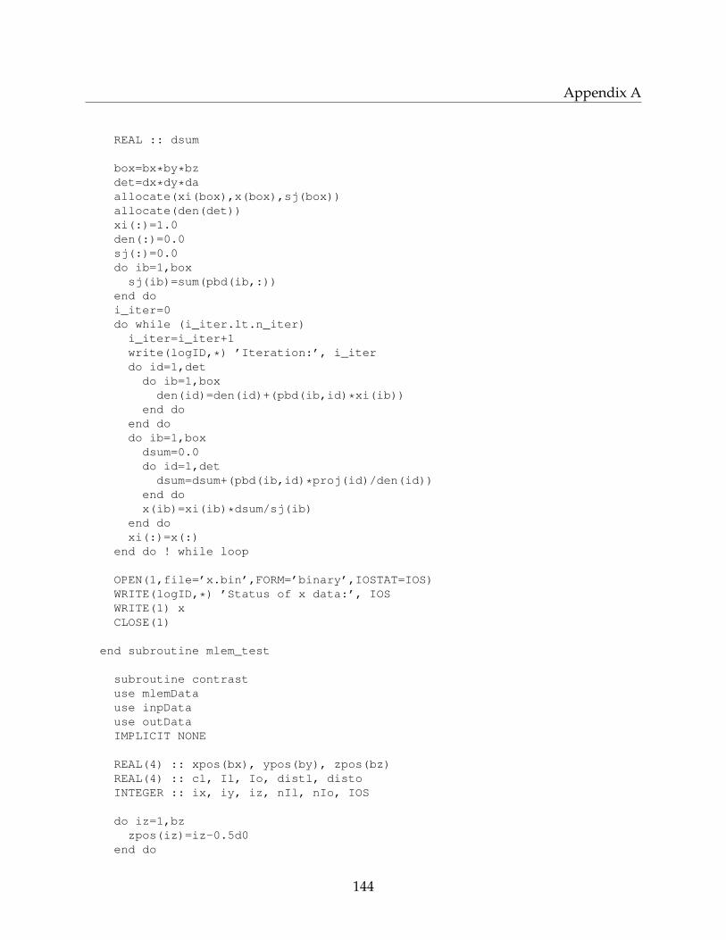
Appendix A
REAL :: dsum
box=bx*by*bzdet=dx*dy*daallocate(xi(box),x(box),sj(box))allocate(den(det))xi(:)=1.0den(:)=0.0sj(:)=0.0do ib=1,box
sj(ib)=sum(pbd(ib,:))end doi_iter=0do while (i_iter.lt.n_iter)
i_iter=i_iter+1write(logID,*) ’Iteration:’, i_iterdo id=1,det
do ib=1,boxden(id)=den(id)+(pbd(ib,id)*xi(ib))
end doend dodo ib=1,box
dsum=0.0do id=1,det
dsum=dsum+(pbd(ib,id)*proj(id)/den(id))end dox(ib)=xi(ib)*dsum/sj(ib)
end doxi(:)=x(:)
end do ! while loop
OPEN(1,file=’x.bin’,FORM=’binary’,IOSTAT=IOS)WRITE(logID,*) ’Status of x data:’, IOSWRITE(1) xCLOSE(1)
end subroutine mlem_test
subroutine contrastuse mlemDatause inpDatause outDataIMPLICIT NONE
REAL(4) :: xpos(bx), ypos(by), zpos(bz)REAL(4) :: cl, Il, Io, distl, distoINTEGER :: ix, iy, iz, nIl, nIo, IOS
do iz=1,bzzpos(iz)=iz-0.5d0
end do
144
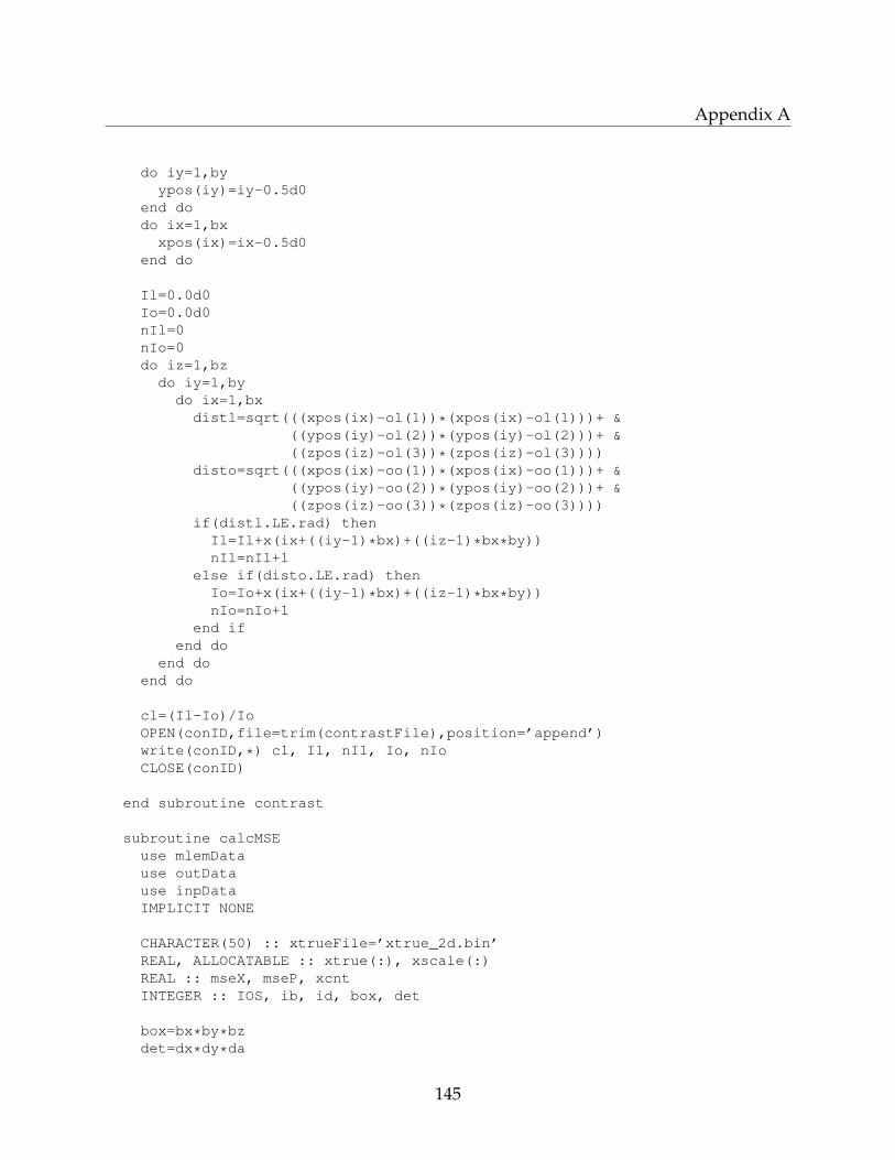
Appendix A
do iy=1,byypos(iy)=iy-0.5d0
end dodo ix=1,bx
xpos(ix)=ix-0.5d0end do
Il=0.0d0Io=0.0d0nIl=0nIo=0do iz=1,bz
do iy=1,bydo ix=1,bxdistl=sqrt(((xpos(ix)-ol(1))*(xpos(ix)-ol(1)))+ &
((ypos(iy)-ol(2))*(ypos(iy)-ol(2)))+ &((zpos(iz)-ol(3))*(zpos(iz)-ol(3))))
disto=sqrt(((xpos(ix)-oo(1))*(xpos(ix)-oo(1)))+ &((ypos(iy)-oo(2))*(ypos(iy)-oo(2)))+ &((zpos(iz)-oo(3))*(zpos(iz)-oo(3))))
if(distl.LE.rad) thenIl=Il+x(ix+((iy-1)*bx)+((iz-1)*bx*by))nIl=nIl+1
else if(disto.LE.rad) thenIo=Io+x(ix+((iy-1)*bx)+((iz-1)*bx*by))nIo=nIo+1
end ifend do
end doend do
cl=(Il-Io)/IoOPEN(conID,file=trim(contrastFile),position=’append’)write(conID,*) cl, Il, nIl, Io, nIoCLOSE(conID)
end subroutine contrast
subroutine calcMSEuse mlemDatause outDatause inpDataIMPLICIT NONE
CHARACTER(50) :: xtrueFile=’xtrue_2d.bin’REAL, ALLOCATABLE :: xtrue(:), xscale(:)REAL :: mseX, mseP, xcntINTEGER :: IOS, ib, id, box, det
box=bx*by*bzdet=dx*dy*da
145

Appendix A
mseX=0mseP=0ALLOCATE(xtrue(box),xscale(box))OPEN(1,file=trim(xtrueFile),form=’binary’,IOSTAT=IOS)READ(1) xtrueCLOSE(1)xcnt=sum(xtrue)xscale(:)=x(:)*xcnt/sum(x)do ib=1,box
if(xtrue(ib).ne.0.AND.xscale(ib).ne.0) thenmseX=mseX+((xscale(ib)-xtrue(ib))*(xscale(ib)-xtrue(ib)))
end ifend domseX=mseX/boxdo id=1,det
if(proj(id).ne.0.AND.den(id).ne.0) thenmseP=mseP+((den(id)-proj(id))*(den(id)-proj(id)))
end ifend domseP=mseP/detOPEN(mseID,file=trim(mseFile),position=’append’)WRITE(mseID,*) mseX, msePCLOSE(mseID)
end subroutine calcMSE
146
Appendix B
TITAN-IR Input and Features
B.1 Reconstruction Input Block
The standard TITAN input file consists of input blocks for transport parameters, geom-
etry, material distribution, source distribution, cross-section data, boundary conditions
and tolerances, and SPECT parameters. A new input block was added to the TITAN-IR
input file to allow the user to specify reconstruction parameters and is shown in Fig. B.1
with example parameters. The first keyword, rectyp, specifies the maximum number of it-
erations to be done and the number of subsets for OS-EM reconstruction. phadim contains
the x, y, and z voxel dimensions of the reconstruction phantom. The phadim keyword
matches the relevant dimensions of the system matrix, but does not have to match the
dimensions of the TITAN phantom model. This allows for a more refined meshing in
the SPECT simulation, which numerics may require for some cases, while maintaining
147
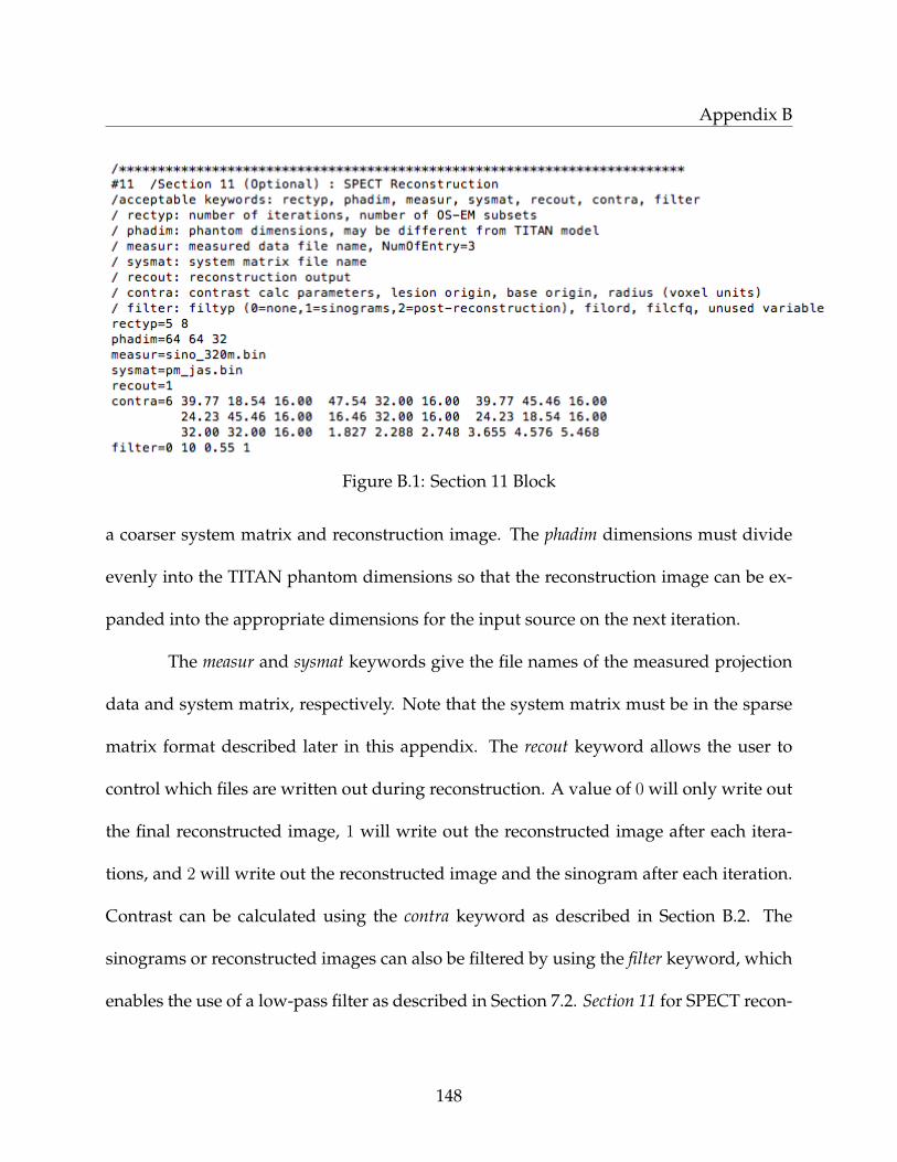
Appendix B
Figure B.1: Section 11 Block
a coarser system matrix and reconstruction image. The phadim dimensions must divide
evenly into the TITAN phantom dimensions so that the reconstruction image can be ex-
panded into the appropriate dimensions for the input source on the next iteration.
The measur and sysmat keywords give the file names of the measured projection
data and system matrix, respectively. Note that the system matrix must be in the sparse
matrix format described later in this appendix. The recout keyword allows the user to
control which files are written out during reconstruction. A value of 0 will only write out
the final reconstructed image, 1 will write out the reconstructed image after each itera-
tions, and 2 will write out the reconstructed image and the sinogram after each iteration.
Contrast can be calculated using the contra keyword as described in Section B.2. The
sinograms or reconstructed images can also be filtered by using the filter keyword, which
enables the use of a low-pass filter as described in Section 7.2. Section 11 for SPECT recon-
148

Appendix B
struction can only be used if Section 10 for SPECT simulation is also present in the input
file.
B.2 Contrast
Contrast is important in determining if an observer can properly interpret the medical im-
age and can assist in determining reconstruction convergence. The contra keyword allows
the user to specify contrast calculations for a variable number of circular lesions. The first
entry gives the number of lesions and is followed by the origin, in units of voxels, of each
lesion. Next the origin of the reference background intensity is given and finally the ra-
dius, in units of voxels, corresponding to each lesion is listed. The reference background
origin is used for calculating the contrast of all lesions, but the background region radius
is adjusted to match the each lesion. The contrast is calculated using Eq. B.1
Cl =Il − I0
I0
(B.1)
where Il is the average image intensity in a region of interest, e.g., a lesion, and I0 is the
average reference background intensity, e.g., normal tissue. The largest reference back-
ground region is also used to estimate the background noise in the image. The contrast of
each lesion and the background noise are printed out for every iteration.
149
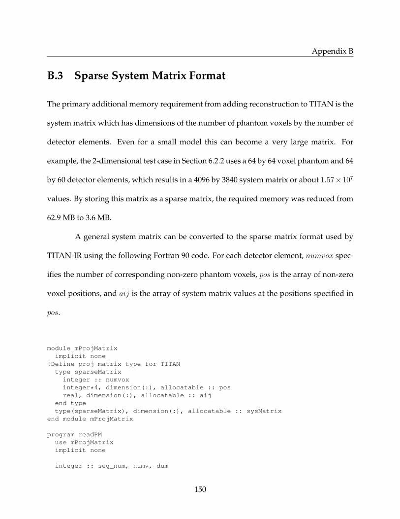
Appendix B
B.3 Sparse System Matrix Format
The primary additional memory requirement from adding reconstruction to TITAN is the
system matrix which has dimensions of the number of phantom voxels by the number of
detector elements. Even for a small model this can become a very large matrix. For
example, the 2-dimensional test case in Section 6.2.2 uses a 64 by 64 voxel phantom and 64
by 60 detector elements, which results in a 4096 by 3840 system matrix or about 1.57×10⁷
values. By storing this matrix as a sparse matrix, the required memory was reduced from
62.9 MB to 3.6 MB.
A general system matrix can be converted to the sparse matrix format used by
TITAN-IR using the following Fortran 90 code. For each detector element, numvox spec-
ifies the number of corresponding non-zero phantom voxels, pos is the array of non-zero
voxel positions, and aij is the array of system matrix values at the positions specified in
pos.
module mProjMatriximplicit none
!Define proj matrix type for TITANtype sparseMatrix
integer :: numvoxinteger*4, dimension(:), allocatable :: posreal, dimension(:), allocatable :: aij
end typetype(sparseMatrix), dimension(:), allocatable :: sysMatrix
end module mProjMatrix
program readPMuse mProjMatriximplicit none
integer :: seg_num, numv, dum
150

Appendix B
integer :: IOS, nbin, i, j, ix, iy, iz, idxinteger :: det, box, pix_det(2), phan_dim(3), num_angreal, dimension(:), allocatable :: pbdcharacter (len=30) :: fileIn
write(*,*) ’Enter the phantom dimensions (x,y,z):’read(*,*) phan_dimwrite(*,*) ’Enter the detector dimensions (x,y,angles):’read(*,*) pix_det, num_angwrite(*,*) ’File to be converted:’read(*,*) fileIn
det=pix_det(1)*pix_det(2)*num_angbox=phan_dim(1)*phan_dim(2)*phan_dim(3)ALLOCATE(pm(det))ALLOCATE(pbd(box))
OPEN(1,file=trim(fileIn),FORM=’binary’,IOSTAT=IOS)
DO j=1,detpbd(:)=0.0numv=0DO i=1,box
READ(1) pbd (i)IF(pbd(i).GT.0) THEN
numv=numv+1END IF
END DOpm(j)%numvox=numvwrite(*,*) ’det:’, j, ’ numv:’, numvALLOCATE(pm(j)%pos(numv),pm(j)%aij(numv))dum=0DO iz=1,phan_dim(3)
DO iy=1,phan_dim(2)DO ix=1,phan_dim(1)idx=((iz-1)*phan_dim(1)*phan_dim(2))+((iy-1)*phan_dim(1))+ixIF(pbd(idx).GT.0) THEN
dum=dum+1pm(j)%pos(dum)=((phan_dim(3)-iz)*phan_dim(1)*phan_dim(2))+((iy-1)*phan_dim(1))+ixpm(j)%aij(dum)=pbd(idx)
END IFEND DO
END DOEND DO
END DOCLOSE(1)
OPEN(1,file=’sparse.bin’,FORM=’binary’,IOSTAT=IOS)DO j=1,det
WRITE(1) pm(j)%numvoxDO i=1,pm(j)%numvox
151

Appendix B
WRITE(1) pm(j)%pos(i), pm(j)%aij(i)END DO
END DOCLOSE(1)
DEALLOCATE(pbd,pm)
end program readPM
152