Introduction to Hypothesis Testing

OPRE 6301

Motivation . . .

The purpose of hypothesis testing is to determine whether

there is enough statistical evidence in favor of a certain

belief, or hypothesis, about a parameter.

Examples:

Is there statistical evidence, from a random sample of

potential customers, to support the hypothesis that

more than 10% of the potential customers will pur-

chase a new product?

Is a new drug effective in curing a certain disease? A

sample of patients is randomly selected. Half of them

are given the drug while the other half are given a

placebo. The conditions of the patients are then mea-

sured and compared.

These questions/hypotheses are similar in spirit to the

discrimination example studied earlier. Below, we pro-

vide a basic introduction to hypothesis testing.

1

Criminal Trials . . .

The basic concepts in hypothesis testing are actually quite

analogous to those in a criminal trial.

Consider a person on trial for a “criminal” offense in theUnited States. Under the US system a jury (or sometimesjust the judge) must decide if the person is innocent orguilty while in fact the person may be innocent or guilty.These combinations are summarized in the table below.

Person is:

Innocent Guilty

Jury Says: Innocent No Error Error

Guilty Error No Error

Notice that there are two types of errors. Are both of

these errors equally important? Or, is it as bad to decide

that a guilty person is innocent and let them go free as

it is to decide an innocent person is guilty and punish

them for the crime? Or, is a jury supposed to be totally

objective, not assuming that the person is either innocent

or guilty and make their decision based on the weight of

the evidence one way or another?

2

In a criminal trial, there actually is a favored assump-

tion, an initial bias if you will. The jury is instructed to

assume the person is innocent, and only decide that the

person is guilty if the evidence convinces them of such.

When there is a favored assumption, the presumed in-

nocence of the person in this case, and the assumption is

true, but the jury decides it is false and declares that the

person is guilty, we have a so-called Type I error.

Conversely, if the favored assumption is false, i.e., the

person is really guilty, but the jury declares that it is

true, that is that the person is innocent, then we have a

so-called Type II error.

3

Thus,

Favored Assumption: Person is Innocent

Person is:

Innocent Guilty

Jury Says: Innocent No Error Type II Error

Guilty Type I Error No Error

In some countries, the favored assumption is that the

person is guilty. In this case the roles of the Type I and

Type II errors would reverse to yield the following table.

Favored Assumption: Person is Guilty

Person is:

Innocent Guilty

Jury Says: Innocent No Error Type I Error

Guilty Type II Error No Error

4

Let us assume that the favored assumption is that the per-

son is innocent. Assume further that in order to declare

the person guilty, the jury must find that the evidence

convinces them beyond a reasonable doubt.

Let

α = P (Type I Error)

= P (Jury Decides Guilty | Person is Innocent ) .

Then, “beyond a reasonable doubt” means that we should

keep α small. For the alternative error, let

β = P (Type II Error)

= P (Jury Decides Innocent | Person is Guilty ) .

Clearly, we would also like to keep β small.

It is important to realize that the conditional probabil-

ities α and β depend on our decision rule. In other

words, we have control over these probabilities.

5

We can make α = 0 by not convicting anyone; how-

ever, every guilty person would then be released so that

β would then equal 1. Alternatively, we can make β = 0

by convicting everyone; however, every innocent person

would then be convicted so that α equals 1. Although

the relationship between α and β is not simple, it should

be clear that they move in opposite directions.

The conditional probability α allows us to formalize the

concept of “reasonable doubt.” If we set a low threshold

for α, say 0.001, then it will require more evidence to

convict an innocent person. On the other hand, if we

set a higher threshold for α, say 0.1, then less evidence

is required. If mathematics could be precisely applied to

the court-room (which it can’t), then for an acceptable

level/threshold for α, we could attempt to determine how

convincing the evidence would have to be to achieve that

threshold for α. This is precisely what we do in hypothesis

testing. The difference between court-room trials and

hypothesis tests in statistics is that in the latter we could

more easily quantify (due in large part to the central

limit theorem) the relationship between our decision rule

and the resulting α.

6

Testing Statistical Hypotheses . . .

In the case of the jury trial, the favored assumption is that

the person is innocent. In statistical inference, one also

works with a favored assumption. This favored assump-

tion is called the null hypothesis, which we will denote

by H0. The “alternative” (or antithesis) to the null hy-

pothesis is, naturally, called the alternative hypoth-

esis, which we will denote by H1 (or HA). The setup of

these hypotheses depends on the application context.

As an example, consider a manufacturer of computer de-

vices. The manufacturer has a process which coats a

computer part with a material that is supposed to be

100 microns thick (one micron is 1/1000 of a millimeter).

If the coating is too thin, then proper insulation of the

computer device will not occur and it will not function

reliably. Similarly, if the coating is too thick, the device

will not fit properly with other computer components.

7

The manufacturer has calibrated the machine that applies

the coating so that it has an average coating depth of 100

microns with a standard deviation of 10 microns. When

calibrated this way, the process is said to be “in control.”

Any physical process, however, will have a tendency to

drift. Mechanical parts wear out, sprayers clog, etc. Ac-

cordingly, the process must be monitored to make sure

that it is “in control.” How can statistics be applied to

this problem?

In this manufacturing problem, the natural favored as-sumption, or the null hypothesis, is that the process is incontrol. The alternative hypothesis is therefore that theprocess is out of control. The analogy to the jury trial is:

Null Hypothesis: Process is In Control

Alternative Hypothesis: Process is Out of Control

Process is:

In Control Out of Control

We Say: In Control No Error Type II Error

Out of Control Type I Error No Error

8

Observe however that the above null hypothesis is not

sufficiently precise: We need to define what it means to

say that the process is in or out of control.

We shall say that the process is in control if the mean is

100 and out of control if the mean is not equal to 100.

Thus,

H0 : µ = 100

H1 : µ 6= 100

and we now have:

Null Hypothesis: µ = 100

Alternative Hypothesis: µ 6= 100

Mean:

Is 100 Is Not 100

We Say: Mean is 100 No Error Type II Error

Mean is not 100 Type I Error No Error

9

The next step is to define reasonable doubt, or equiva-

lently a threshold for α. This is an individual choice but,

like the construction of a confidence interval, the two most

commonly-used values are 0.05 (or about a one in twenty

chance) and 0.01 (or about a one in one hundred chance).

Let us pick a threshold of 0.05. It is common practice to

abbreviate this statement simply as: Let α = 0.05.

As in a criminal trial, we must now collect evidence. In a

statistical analysis, the evidence comes from data. In or-

der to use data as evidence for or against the null hypoth-

esis, we need to know how to appropriately summarize

information contained in the data. Since our hypothesis

is a statement about the population mean, it is natural

to use the sample mean as our evidence.

Suppose we intend to take a sample of (say) 4 chips and

compute the sample mean X̄ . How do we assess the

evidence to be manifested in the value of X̄?

10

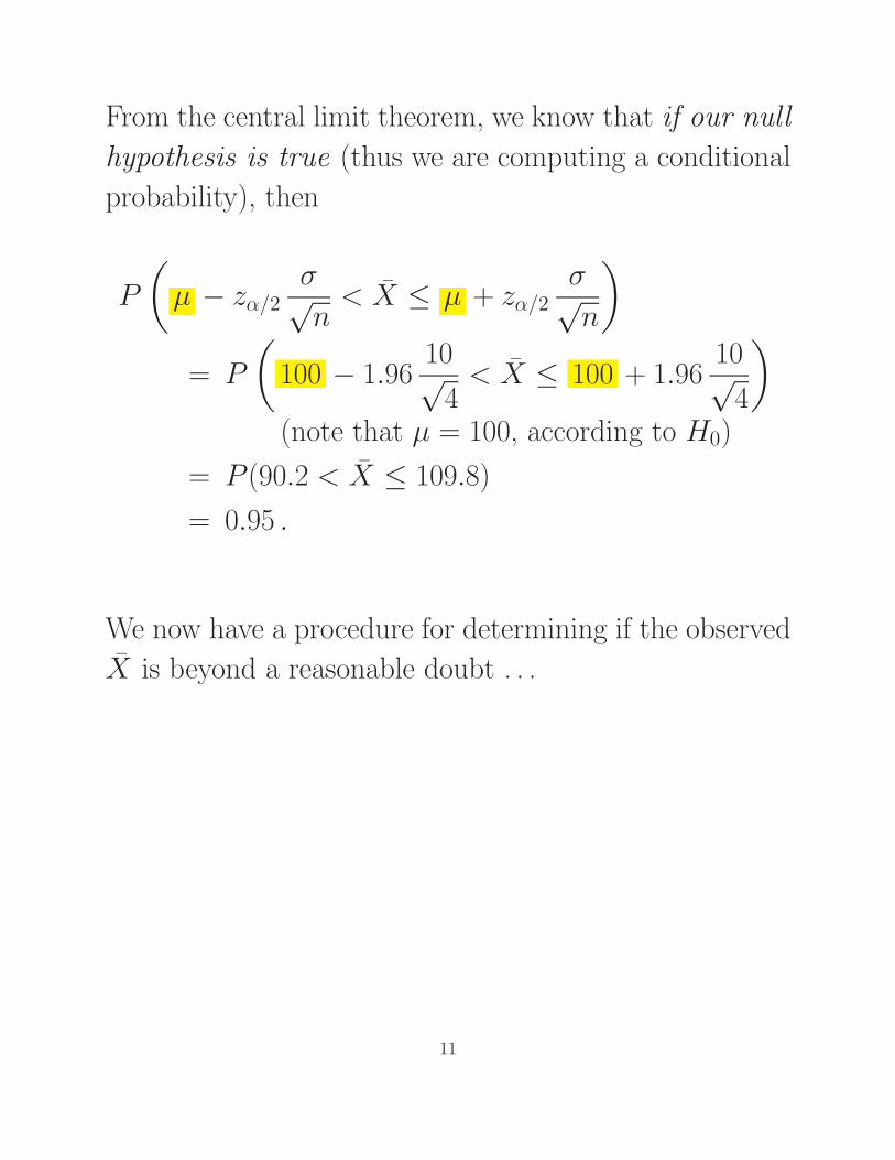
From the central limit theorem, we know that if our null

hypothesis is true (thus we are computing a conditional

probability), then

P

(

µ − zα/2σ√n

< X̄ ≤ µ + zα/2σ√n

)

= P

(

100 − 1.9610√

4< X̄ ≤ 100 + 1.96

10√4

)

(note that µ = 100, according to H0)

= P (90.2 < X̄ ≤ 109.8)

= 0.95 .

We now have a procedure for determining if the observed

X̄ is beyond a reasonable doubt . . .

11

Procedure

(a) Compute X̄ .

(b) If X̄ falls between 90.2 and 109.8, then this is what

would happen approximately 95% of the time if the

manufacturing process was in control. We would there-

fore declare that it is in control.

(c) If X̄ falls outside the range of (90.2, 109.8), then ei-

ther one of two things could have happened: (I) the

process is in control and it just fell outside by chance

(which will happen about 5% of time); or (II) the

process is out of control. While we can’t be sure which

is the case, but since the evidence is beyond a reason-

able doubt, we would declare that the manufacturing

process is out of control.

12

It is important to realize that under (b), just because

you decide/declare that the process is in control, it does

not mean that the process in fact is in control. Similarly

under (c), if you decide/declare that the process is out of

control, it might just be a random occurrence of an X̄

outside the control limits; and this would happen with

probability 0.05, assuming that H0 is true.

The procedure described above is an example of quality

control. To ensure that a manufacturing process is in

control, one could collect data (say) daily and check the

observed X̄s against the control limits to determine if the

process is performing as it should be.

13

Summary

An often-heard statement is that “Statistics has proved

such and such.” There is of course also the even stronger

statement that “Statistics can prove anything.” In fact,

now that you have examined the structure of statistical

logic, it should be clear that one does not “prove” any-

thing. Rather, we are only looking at consistency or in-

consistency between the observed data and the proposed

hypotheses.

If the observed data is “consistent” with the null hypothe-

sis (in our example, this means that the sample mean falls

between 90.2 and 109.8), then instead of “proving the hy-

pothesis true,” the proper interpretation is that there is

no reason to doubt that the null hypothesis is true.

Similarly, if the observed data is “inconsistent” with the

null hypothesis (in our example, this means that the sam-

ple mean falls outside the interval (90.2, 109.8)), then

either a rare event has occurred (rareness is judged by

thresholds 0.05 or 0.01) and the null hypothesis is true,

or in fact the null hypothesis is not true.

14

One-Tail Tests . . .

In the quality-control problem, we compared X̄ against a

pair of upper and lower control limits. This is an example

of a two-tail test. Below, we will discuss an example of

a one-tail test.

The manager of a department store is interested in the

cost effectiveness of establishing a new billing system for

the store’s credit customers. After a careful analysis,

she determines that the new system is justified only if

the mean monthly account size is more than $170 . The

manager wishes to find out if there is sufficient statistical

support for this.

The manager takes a random sample of 400 monthly ac-

counts. The sample mean turns out to be $178. Historical

data indicate that the standard deviation of monthly ac-

counts is about $65.

15

Observe that what we are trying to find out is whether or

not there is sufficient support for the hypothesis that the

mean monthly accounts are “more than $170.” The stan-

dard procedure is then to let µ > 170 be the alternative

hypothesis. For this reason, the alternative hypothesis is

also often referred to as the research hypothesis.

It follows that the null hypothesis should be defined as

µ = 170. Note that we do not use µ ≤ 170 as the null

hypothesis; this is because the null hypothesis must be

precise enough for us to determine a “unique” sampling

distribution. The choice µ = 170 also gives H0, our fa-

vored assumption, the least probability of being rejected.

Thus,

H0 : µ = 170

H1 : µ > 170

where H1 is what we want to determine and H0 spec-

ifies a single value for the parameter of interest.

How do we test such a pair of hypotheses? There are two

equivalent approaches . . .

16

Rejection-Region Approach

This approach is similar to what we did in the quality-

control problem. However, we will just have one “upper”

control limit, and hence the name one-tail test.

Clearly, if the sample mean is “large” relative to 170,

i.e., if X̄ > X̄L for a suitably-chosen control limit X̄L,

then we should reject the null hypothesis in favor of the

alternative.

Pictorially, this means that for a given α, we wish to find

X̄L such that:

L1 7 0x =�17

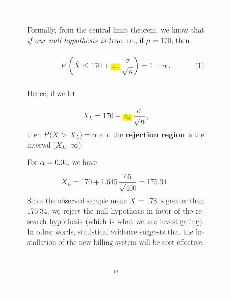
Formally, from the central limit theorem, we know that

if our null hypothesis is true, i.e., if µ = 170, then

P

(

X̄ ≤ 170 + zασ√n

)

= 1 − α . (1)

Hence, if we let

X̄L = 170 + zασ√n

,

then P (X̄ > X̄L) = α and the rejection region is the

interval (X̄L, ∞).

For α = 0.05, we have

X̄L = 170 + 1.64565√400

= 175.34 .

Since the observed sample mean X̄ = 178 is greater than

175.34, we reject the null hypothesis in favor of the re-

search hypothesis (which is what we are investigating).

In other words, statistical evidence suggests that the in-

stallation of the new billing system will be cost effective.

18

The critical-region approach can also be implemented via

the standardized variable Z, as follows.

Observe that (1) is equivalent to:

P

(

Z =X̄ − 170

σ/√

n≤ zα

)

= 1 − α . (2)

Hence, P (Z > zα ) = α and, in terms of Z, the rejection

region is the interval (zα, ∞).

For α = 0.05, we have

Z =178 − 170

65/√

400= 2.46 .

Since 2.46 is greater than zα = 1.645, we reject H0 in

favor of H1. This conclusion is of course the same as the

previous one.

19

p -Value Approach

The concept of p-values introduced earlier can also be

used to conduct hypothesis tests. In this context, the p-

value is defined as the probability of observing any test

statistic that is at least as extreme as the one computed

from a sample, given that the null hypothesis is true.

In the monthly account size example, the p-value associ-

ated with the given sample mean 178 is:

P(

X̄ ≥ 178 | µ = 170)

= P

(

Z ≥ 178 − 170

65/√

400

)

= P (Z ≥ 2.4615)

= 1 − P (Z ≤ 2.4615)

= 0.0069 ,

where the last equality comes from

P (Z ≤ 2.4615) = NORMSDIST(2.4615)

= 0.9931 .

20

Pictorially, we have:

1 7 0x =� 1 7 8x =The p-value

It is illuminating to observe that under H1 with a µ > 170

but still with the same sample mean 178 (the brown curve

below), we would have a higher p-value:

1 7 8x =1 7 0:H x0 =� 1 7 0:H x1 >(21

The p-value therefore provides explicit information about

the amount of statistical evidence that supports the al-

ternative hypothesis. More explicitly, the smaller the p-

value, the stronger the statistical evidence against the null

hypothesis is.

For our problem, since the p-value 0.0069 is (substan-

tially) below the specified α = 0.05, the null hypothesis

should be rejected in favor of the alternative hypothesis.

This conclusion again is the same as before.

In general, we have the following guidelines:

— If the p-value is less than 1%, there is overwhelming

evidence that supports the alternative hypothesis.

— If the p-value is between 1% and 5%, there is a strong

evidence that supports the alternative hypothesis.

— If the p-value is between 5% and 10% there is a weak

evidence that supports the alternative hypothesis.

— If the p-value exceeds 10%, there is no evidence that

supports the alternative hypothesis.

22

Our account-size problem is an example of a right-tail

test. Depending on what we are trying to find out, we

could also conduct a left-tail test, i.e., consider a hy-

potheses pair of the form:

H0 : µ = µ0

H1 : µ < µ0

Clearly, the method is similar.

In general, we have:

23

Calculating and Controlling β . . .

It is important to have a good understanding of the rela-

tionship between Type I and Type II errors; that is, how

the probability of a Type II error is calculated and its

interpretation.

Consider again the account size problem. Recall that a

Type II error occurs when a false null hypothesis is not

rejected. In that example, we would not reject the null

hypothesis if the sample mean X̄ is less than or equal to

the critical value X̄L = 175.34. It follows that

β = P (X̄ ≤ 175.34 | H0 is false) .

Observe that to compute β, one has to work with a spe-

cific value of µ that is greater than what H0 states, i.e.,

170. For the sake of discussion, let us pick 180 . For this

choice, we have

β = P (X̄ ≤ 175.34 | µ = 180 ) .

24

The central limit theorem then tells us that

β = P

(

Z ≤ 175.34 − 180

65/√

400

)

= P (Z ≤ −1.43)

= 0.0764 .

Pictorially, this means that:O u r o r i g i n a l h y p o t h e s i s …o u r n e w a s s u m p t i o n …

X̄

X̄

25

Observe that decreasing the significance level α will re-

sult in an increase in β, and vice versa. Alternatively,

this is equivalent to saying that shifting X̄L to the right

(to decrease α) will result in a larger β, and vice versa.

Pictorially, we have

X̄X̄

X̄ X̄

It is clear from the above figure that α and β move in

opposite directions. An important question then is: Is it

possible to decrease β, for a given level of α?

26

The answer is that the shape of the sampling distribution

must change, and for that to happen, we need to increase

the sample size n:

Lx = = 1 8 0= = 1 7 0 Lx

d o e s n o t c h a n g e ,b u t b e c o m e s s m a l l e r

Formally, . . .

27

Suppose the sample size n is increased to 1,000; then,

X̄L = µ + zασ√n

= 170 + 1.64565√1000

= 173.38

and hence, for the same alternative µ = 180 ,

β = P

(

Z ≤ 173.38 − 180

65/√

1000

)

= P (Z ≤ −3.22) ≈ 0 .

That is, while maintaining the same α = 0.05 (and as-

suming that µ = 180), the probability of committing a

Type II error has been reduced to essentially zero!

The conditional probability 1−β is called the power of

a test; it is the probability of taking the correct action

of rejecting the null hypothesis when it is false. By in-

creasing n, we can improve the power of a test. For the

same α and the same n, the power of test is also used to

choose between different tests; a “more powerful” test is

one that yields the correct action with greater frequency.

28