Probability

OPRE 6301

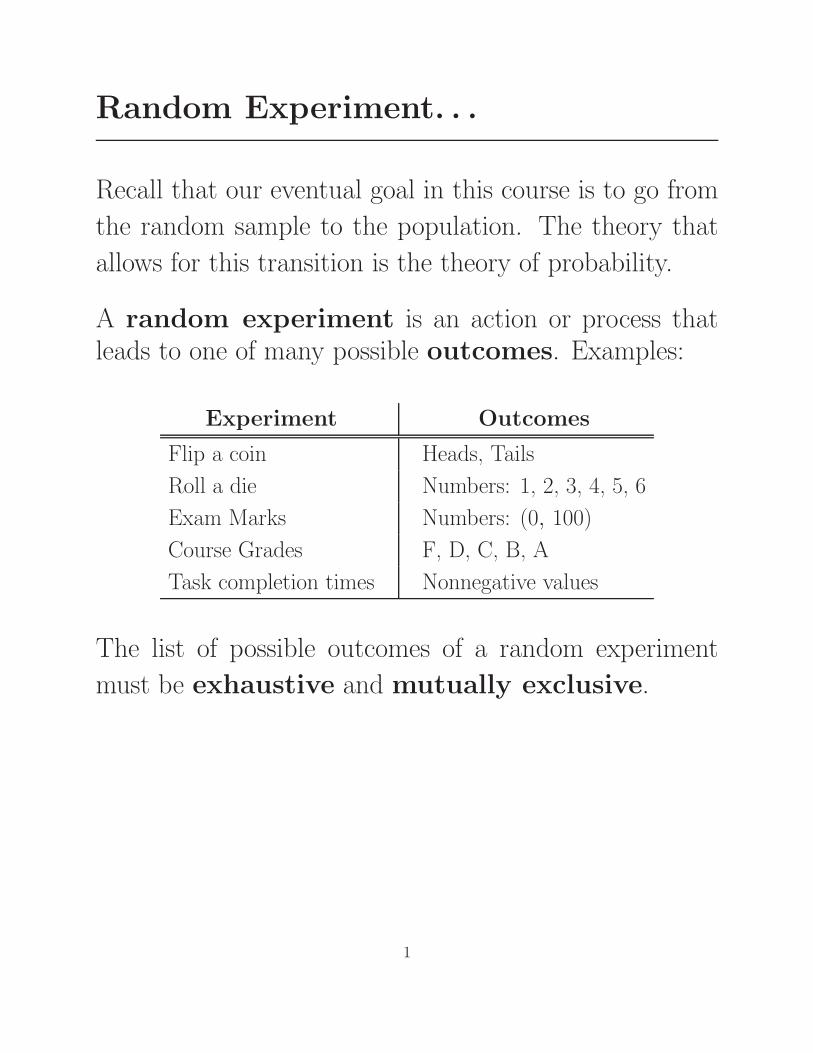
Random Experiment. . .

Recall that our eventual goal in this course is to go from

the random sample to the population. The theory that

allows for this transition is the theory of probability.

A random experiment is an action or process thatleads to one of many possible outcomes. Examples:

Experiment Outcomes

Flip a coin Heads, Tails

Roll a die Numbers: 1, 2, 3, 4, 5, 6

Exam Marks Numbers: (0, 100)

Course Grades F, D, C, B, A

Task completion times Nonnegative values

The list of possible outcomes of a random experiment

must be exhaustive and mutually exclusive.

1

Sample Space. . .

The set of all possible outcomes of an experiment is called

the sample space.

We will denote the outcomes by O1, O2, . . . , and the

sample space by S. Thus, in set-theory notation,

S = {O1, O2, . . .}

2

Events. . .

An individual outcome in the sample space is called a

simple event, while. . .

An event is a collection or set of one or more simple

events in a sample space.

Example: Roll of a Die

S = {1, 2, · · · , 6}

Simple Event: The outcome “3”.

Event: The outcome is an even number (one of 2, 4, 6)

Event: The outcome is a low number (one of 1, 2, 3)

3

Assigning Probabilities. . .

Requirements

Given a sample space S = {O1, O2, . . .}, the probabil-

ities assigned to events must satisfy these requirements:

1. The probability of any event must be nonnegative,

e.g., P (Oi) ≥ 0 for each i.

2. The probability of the entire sample space must be 1,

i.e., P (S) = 1.

3. For two disjoint events A and B, the probability of

the union of A and B is equal to the sum of the

probabilities of A and B, i.e.,

P (A ∪ B) = P (A) + P (B) .

Approaches

There are three ways to assign probabilities to events:

classical approach, relative-frequency approach,

subjective approach. Details. . .

4

Classical Approach. . .

If an experiment has n simple outcomes, this method

would assign a probability of 1/n to each outcome. In

other words, each outcome is assumed to have an equal

probability of occurrence.

This method is also called the axiomatic approach.

Example 1: Roll of a Die

S = {1, 2, · · · , 6}

Probabilities: Each simple event has a 1/6 chance of

occurring.

Example 2: Two Rolls of a Die

S = {(1, 1), (1, 2), · · · , (6, 6)}

Assumption: The two rolls are “independent.”

Probabilities: Each simple event has a (1/6) · (1/6) =

1/36 chance of occurring.

5

Relative-Frequency Approach. . .

Probabilities are assigned on the basis of experimentation

or historical data.

Formally, Let A be an event of interest, and assume that

you have performed the same experiment n times so that

n is the number of times A could have occurred. Fur-

ther, let nA be the number of times that A did occur.

Now, consider the relative frequency nA/n. Then, in

this method, we “attempt” to define P (A) as:

P (A) = limn→∞

nA

n.

The above can only be viewed as an attempt because it

is not physically feasible to repeat an experiment an infi-

nite number of times. Another important issue with this

definition is that two sets of n experiments will typically

result in two different ratios. However, we expect the

discrepancy to converge to 0 for large n. Hence, for large

n, the ratio nA/n may be taken as a reasonable approxi-

mation for P (A).

6

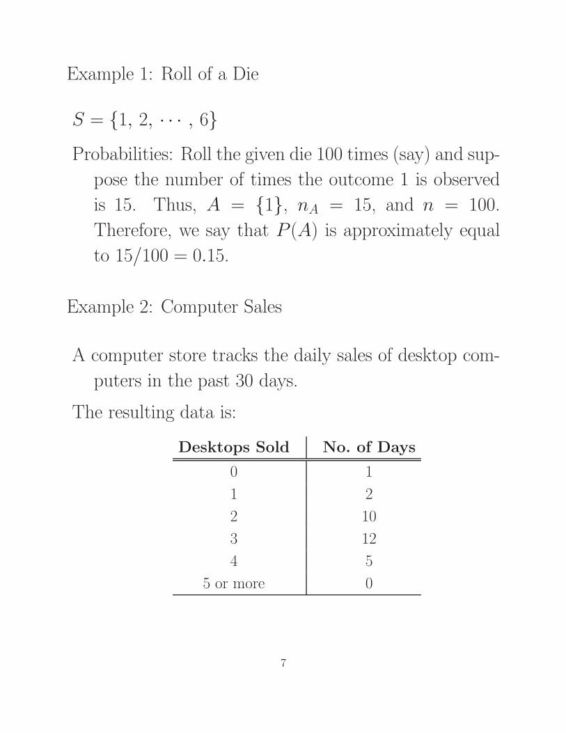
Example 1: Roll of a Die

S = {1, 2, · · · , 6}

Probabilities: Roll the given die 100 times (say) and sup-

pose the number of times the outcome 1 is observed

is 15. Thus, A = {1}, nA = 15, and n = 100.

Therefore, we say that P (A) is approximately equal

to 15/100 = 0.15.

Example 2: Computer Sales

A computer store tracks the daily sales of desktop com-

puters in the past 30 days.

The resulting data is:

Desktops Sold No. of Days

0 1

1 2

2 10

3 12

4 5

5 or more 0

7

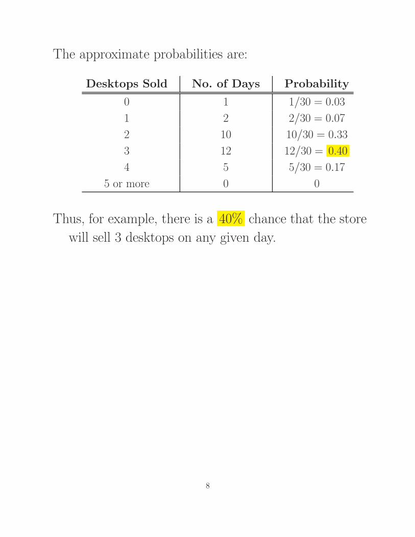
The approximate probabilities are:

Desktops Sold No. of Days Probability

0 1 1/30 = 0.03

1 2 2/30 = 0.07

2 10 10/30 = 0.33

3 12 12/30 = 0.40

4 5 5/30 = 0.17

5 or more 0 0

Thus, for example, there is a 40% chance that the store

will sell 3 desktops on any given day.

8

Subjective Approach. . .

In the subjective approach, we define probability as the

degree of belief that we hold in the occurrence of an

event. Thus, judgment is used as the basis for assigning

probabilities.

Notice that the classical approach of assigning equal prob-

abilities to simple events is, in fact, also based on judg-

ment.

What is somewhat different here is that the use of the

subjective approach is usually limited to experiments that

are unrepeatable.

9

Example 1: Horse Race

Consider a horse race with 8 horses running. What is the

probability for a particular horse to win? Is it reason-

able to assume that the probability is 1/8? Note that

we can’t apply the relative-frequency approach.

People regularly place bets on the outcomes of such “one-

time” experiments based on their judgment as to how

likely it is for a particular horse to win. Indeed, having

different judgments is what makes betting possible!

Example 2: Stock Price

What is the probability for a particular stock to go up to-

morrow? Again, this “experiment” can’t be repeated,

and we can’t apply the relative-frequency approach.

Sophisticated models (that rely on past data) are often

used to make such predictions, as blindly following

ill-founded judgments is often dangerous.

10

Basic Rules of Probability. . .

All three definitions of probability must follow the same

rules. We now describe some basic concepts and rules.

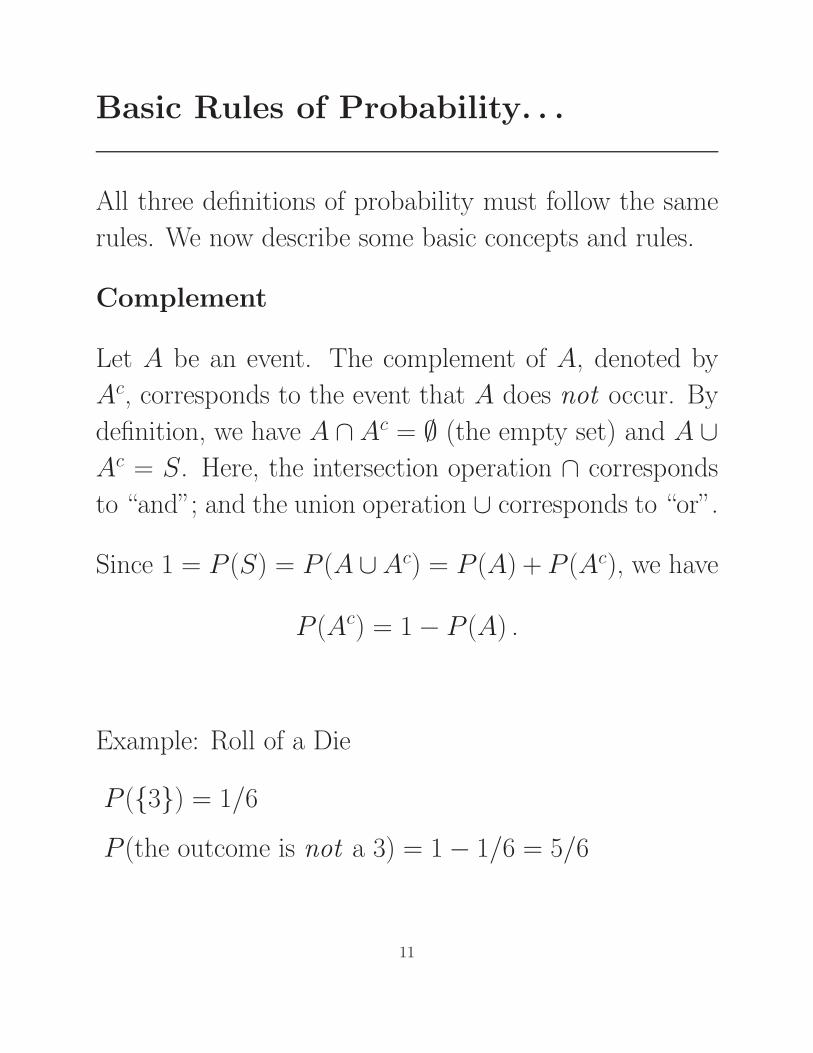
Complement

Let A be an event. The complement of A, denoted by

Ac, corresponds to the event that A does not occur. By

definition, we have A ∩ Ac = ∅ (the empty set) and A ∪

Ac = S. Here, the intersection operation ∩ corresponds

to “and”; and the union operation ∪ corresponds to “or”.

Since 1 = P (S) = P (A∪Ac) = P (A) + P (Ac), we have

P (Ac) = 1 − P (A) .

Example: Roll of a Die

P ({3}) = 1/6

P (the outcome is not a 3) = 1 − 1/6 = 5/6

11

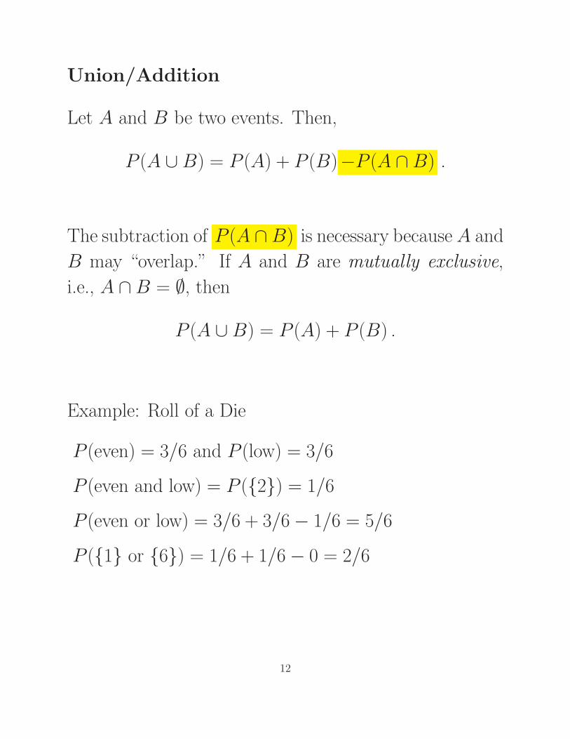
Union/Addition

Let A and B be two events. Then,

P (A ∪ B) = P (A) + P (B)−P (A ∩ B) .

The subtraction of P (A ∩ B) is necessary because A and

B may “overlap.” If A and B are mutually exclusive,

i.e., A ∩ B = ∅, then

P (A ∪ B) = P (A) + P (B) .

Example: Roll of a Die

P (even) = 3/6 and P (low) = 3/6

P (even and low) = P ({2}) = 1/6

P (even or low) = 3/6 + 3/6 − 1/6 = 5/6

P ({1} or {6}) = 1/6 + 1/6 − 0 = 2/6

12

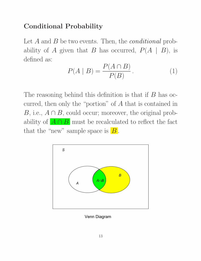
Conditional Probability

Let A and B be two events. Then, the conditional prob-

ability of A given that B has occurred, P (A | B), is

defined as:

P (A | B) =P (A ∩ B)

P (B). (1)

The reasoning behind this definition is that if B has oc-

curred, then only the “portion” of A that is contained in

B, i.e., A ∩ B, could occur; moreover, the original prob-

ability of A ∩ B must be recalculated to reflect the fact

that the “new” sample space is B .

Venn Diagram

A B

B

A

S

13

Example: Pick a Card from a Deck

Suppose a card is drawn randomly from a deck and found

to be an Ace. What is the conditional probability for

this card to be Spade Ace?

A = Spade Ace

B = an Ace

A ∩ B = Spade Ace

P (A) = 1/52; P (B) = 4/52; and P (A ∩ B) = 1/52

Hence,

P (A | B) =1/52

4/52=

1

4.

14

Multiplication

The multiplication rule is used to calculate the joint

probability of two events. It is simply a rearrangement of

the conditional probability formula; see (1). Formally,

P (A ∩ B) = P (A | B)P (B) ;

or,

P (A ∩ B) = P (B | A)P (A) .

Example 1: Drawing a Spade Ace

A = an Ace

B = a Spade

A ∩ B = the Spade Ace

P (B) = 13/52; P (A | B) = 1/13

Hence,

P (A ∩ B) = P (A | B)P (B)

=1

13·13

52=

1

52.

15

Example 2: Selecting Students

A statistics course has seven male and three female stu-

dents. The professor wants to select two students at

random to help her conduct a research project. What

is the probability that the two students chosen are

female?

A = the first student selected is female

B = the second student selected is female

A ∩ B = both chosen students are female

P (A) = 3/10; P (B | A) = 2/9

Hence,

P (A ∩ B) = P (B | A)P (A)

=2

9·

3

10

=1

15.

16

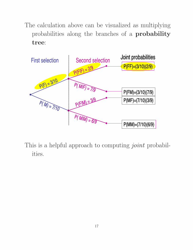
The calculation above can be visualized as multiplying

probabilities along the branches of a probability

tree:

First selection Second selection

P(F) = 3/10

P( M) = 7/10P(F|M) = 3/9

P(F|F) = 2/9

P( M|M) = 6/9

P( M|F) = 7/9P(F) = 3/10

P( M) = 7/10P(F|M) = 3/9

P(F|F) = 2/9

P( M|M) = 6/9

P( M|F) = 7/9

P(FF)=(3/10)(2/9)

P(FM)=(3/10)(7/9)

P(MF)=(7/10)(3/9)

P(MM)=(7/10)(6/9)

Joint probabilities

P(FF)=(3/10)(2/9)

P(FM)=(3/10)(7/9)

P(MF)=(7/10)(3/9)

P(MM)=(7/10)(6/9)

Joint probabilities

This is a helpful approach to computing joint probabil-

ities.

17

Independence

Two events are said to be independent if the occurrence

of either one of the two events does not affect the occur-

rence probability of the other event. This is an important

concept, and is formally stated as: Two events A and B

are independent if

P (A | B) = P (A) ;

or,

P (B | A) = P (B) .

Note that the above is equivalent to

P (A ∩ B) = P (A)P (B) .

Example: Drawings with Replacement

Two balls are successively drawn from an urn that con-

tains seven red balls and three black balls. The first

ball drawn is put back into the urn after noting its

color. What is the probability that the two balls

drawn are both black?

18

A = the first ball drawn is black

B = the second ball drawn is black

A ∩ B = both balls are black

P (A) = 3/10; P (B | A) = P (B) = 3/10, i.e., B and A

are independent

Hence,

P (A ∩ B) = P (B | A)P (A)

=3

10·

3

10

=9

100.

19

Bayes’ Law. . .

Suppose we know the conditional probabilities of an event

for all possible “causes” of the event. We can use this

information to find the probability of the possible cause,

given that this event has occurred.

Example: Multiple-Choice Exam

In a multiple-choice exam, each question has m possible

answers, but only one of them is correct. Suppose a

student adopts the strategy of picking one of the pos-

sible answers randomly whenever he does not know

the correct answer to a question. Assume that the

probability for the student to know the answer to a

question is p.

Suppose the student answered a question correctly. What

is the conditional probability for the student to have

truly known the correct answer?

K = the student truly knows the answer

C = the student answered a question correctly

P (K | C) = ?

20

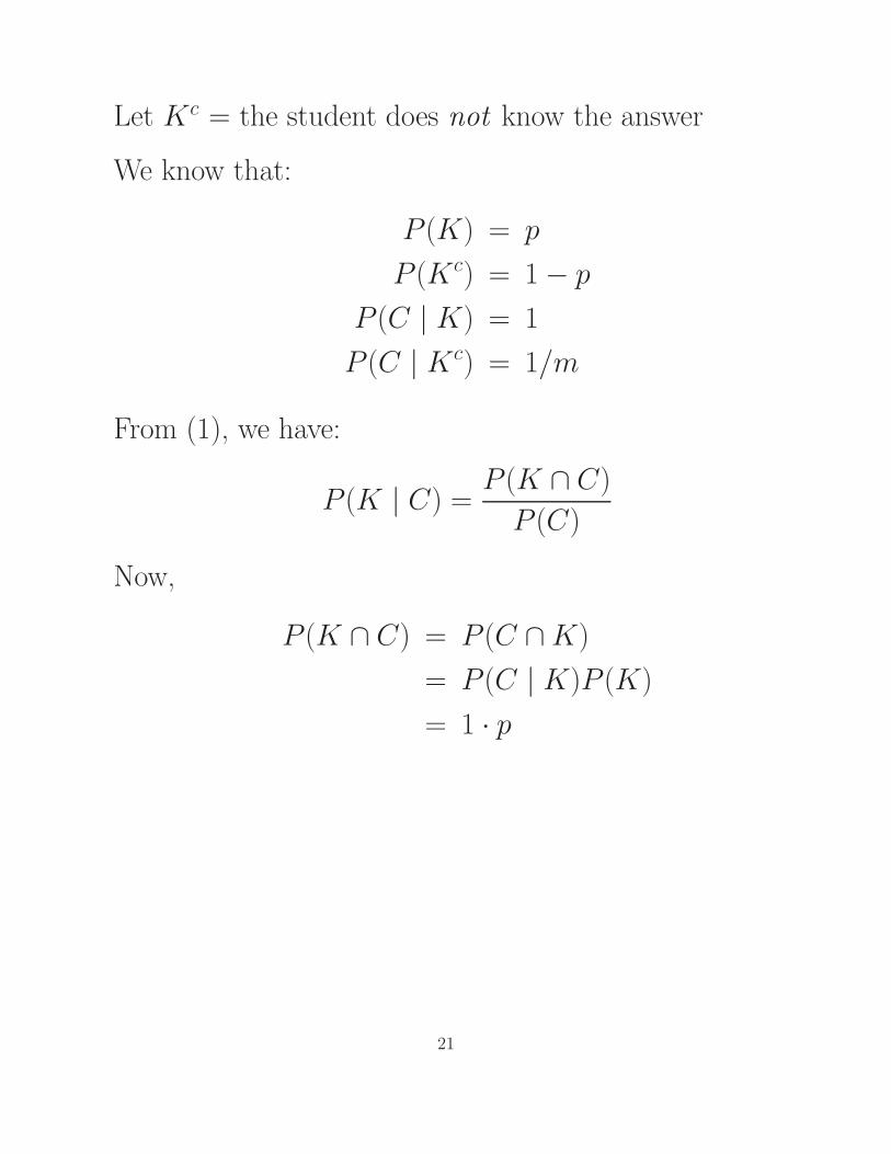
Let Kc = the student does not know the answer

We know that:

P (K) = p

P (Kc) = 1 − p

P (C | K) = 1

P (C | Kc) = 1/m

From (1), we have:

P (K | C) =P (K ∩ C)

P (C)

Now,

P (K ∩ C) = P (C ∩ K)

= P (C | K)P (K)

= 1 · p

21

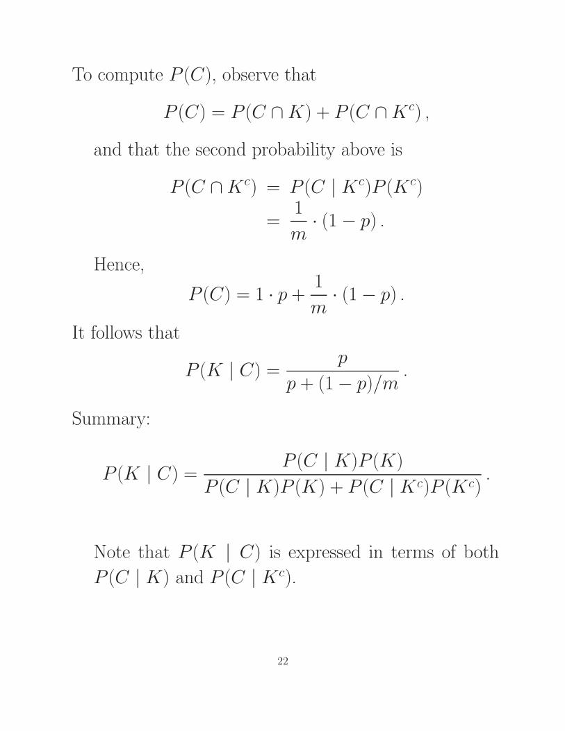
To compute P (C), observe that

P (C) = P (C ∩ K) + P (C ∩ Kc) ,

and that the second probability above is

P (C ∩ Kc) = P (C | Kc)P (Kc)

=1

m· (1 − p) .

Hence,

P (C) = 1 · p +1

m· (1 − p) .

It follows that

P (K | C) =p

p + (1 − p)/m.

Summary:

P (K | C) =P (C | K)P (K)

P (C | K)P (K) + P (C | Kc)P (Kc).

Note that P (K | C) is expressed in terms of both

P (C | K) and P (C | Kc).

22

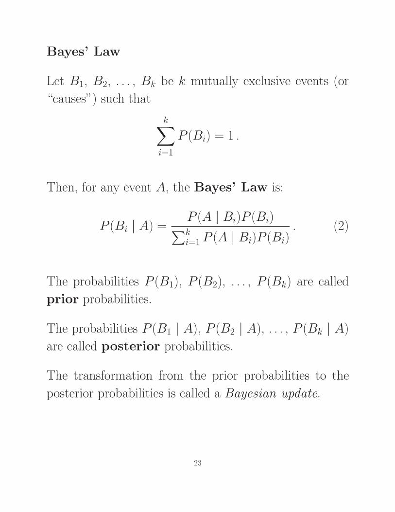
Bayes’ Law

Let B1, B2, . . . , Bk be k mutually exclusive events (or

“causes”) such that

k∑

i=1

P (Bi) = 1 .

Then, for any event A, the Bayes’ Law is:

P (Bi | A) =P (A | Bi)P (Bi)∑ki=1

P (A | Bi)P (Bi). (2)

The probabilities P (B1), P (B2), . . . , P (Bk) are called

prior probabilities.

The probabilities P (B1 | A), P (B2 | A), . . . , P (Bk | A)

are called posterior probabilities.

The transformation from the prior probabilities to the

posterior probabilities is called a Bayesian update.

23

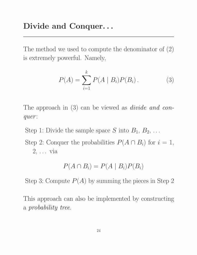
Divide and Conquer. . .

The method we used to compute the denominator of (2)

is extremely powerful. Namely,

P (A) =k∑

i=1

P (A | Bi)P (Bi) . (3)

The approach in (3) can be viewed as divide and con-

quer :

Step 1: Divide the sample space S into B1, B2, . . .

Step 2: Conquer the probabilities P (A ∩ Bi) for i = 1,

2, . . . via

P (A ∩ Bi) = P (A | Bi)P (Bi)

Step 3: Compute P (A) by summing the pieces in Step 2

This approach can also be implemented by constructing

a probability tree.

24