Bounds on Risk-averse Mixed-integer Multi-stage Stochastic
Programming Problems with Mean-CVaR
Ali rfan Mahmuto§ullar , Özlem Çavu³∗, and M. Selim Aktürk
Department of Industrial Engineering, Bilkent University, 06800 Ankara, TURKEY
Abstract
Risk-averse mixed-integer multi-stage stochastic programming forms a class of extremely chal-
lenging problems since the problem size grows exponentially with the number of stages, the problem
is non-convex due to integrality restrictions and the objective function is a dynamic measure of risk.
For this reason, we propose a scenario tree decomposition approach, namely group subproblem ap-
proach, to obtain bounds for such problems with an objective of dynamic mean-CVaR risk measure.
Our approach does not require any special problem structure such as convexity and linearity, there-
fore it can be applied to a wide range of problems. We obtain lower bounds by using dierent
convolution of mean-CVaR risk measures and dierent scenario partition strategies. The upper
bounds are obtained through the use of optimal solutions of group subproblems. Using these lower
and upper bounds, we propose an algorithm for risk-averse mixed-integer multi-stage stochastic
problems with mean-CVaR risk measures. We test the performance of the proposed algorithm on a
multi-stage stochastic lot sizing problem and compare dierent choices of lower bounds and parti-
tion strategies. Comparison of the proposed algorithm and the commercial solver revealed that, on
the average, the proposed algorithm yields 2.58 times stronger bounds compared to a commercial
solver.
Keywords: Stochastic programming; Mixed-integer multi-stage stochastic programming; Dy-
namic measures of risk; CVaR; Bounding.
1 Introduction
In risk-averse stochastic optimization problems, risk measures are used to assess the risk involved
in the decisions made. Due to the structural properties of risk measures, risk-averse models are more
challenging than their risk-neutral counterparts. The multi-stage risk-averse stochastic models are even
more complicated due to their dynamic nature and excessive amount of decision variables. Both the
risk-neutral and risk-averse multi-stage stochastic problems are non-convex when some of the decision
variables are required to be integer valued. Therefore, the solution methods suggested for convex
multi-stage stochastic problems cannot be used to solve these problems.
In this study, we consider risk-averse mixed-integer multi-stage stochastic problems with dynamic
objective functions dened via mean conditional value-at-risk (mean-CVaR). Mean-CVaR is a coherent
measure of risk that has been used in the literature extensively. Coherent measures of risk and their
axiomatic properties are introduced in the pioneering paper by Artzner et al. [1999]. Later, the theory
∗Corresponding author: [email protected]
1
of coherent risk measures are extended by Rockafellar and Uryasev [2002], Ruszczynski and Shapiro
[2006a,b], and references therein.
In a multi-stage decision horizon, risk involved in a stream of random outcomes is considered.
Therefore, dynamic coherent risk measures are introduced to quantify the risk in multi-period models
[see Ruszczynski and Shapiro [2006a,b], Artzner et al. [2007], Pug and Römisch [2007], Kovacevic and
Pug [2009] and references therein].
For the multi-stage stochastic optimization problems with dynamic measures of risk, some exact
solution techniques are suggested under the assumption that the decision variables are continuous.
These techniques, such as stochastic dual dynamic programming (SDDP) (see [Pereira and Pinto,
1991, Shapiro, 2011, Shapiro et al., 2013, Philpott et al., 2013]) and Lagrangian relaxation of nonan-
ticipativity constraints [Collado et al., 2012], rely on the convex structure of the problem, therefore,
they cannot be used to nd an exact solution when some of the decision variables are integer valued.
On the other hand, these methods can be used to obtain lower bounds on the optimal value of multi-
stage stochastic integer problems. Bonnans et al. [2012] propose an extension of SDDP method for the
risk neutral problems with integer variables by relaxing the integrality requirements in the backward
steps of the algorithm. Later, Bruno et al. [2016] extend this approach to risk-averse integer prob-
lems. Similarly, Schultz [2003] use Lagrangian relaxation of nonanticipativity constraints to obtain
lower bounds within a branch-and-bound procedure for risk-neutral multi-stage problems with integer
variables. However, these approaches rely on some restrictive assumptions. SDDP method requires
stagewise independency of random process and the branch-and-bound procedure requires complete
recourse assumptions. Therefore, they cannot be applicable to a wide range of problems.
A recent stream of research proposes an alternative way of obtaining bounds for mixed-integer
multi-stage stochastic problems via a scenario tree decomposition. In that approach, the sample space
is partitioned into subspaces called as groups, and the problem is solved for the scenarios in a group
instead of the original sample space. These smaller problems are called as group subproblems. Sandkç
et al. [2013] propose a group subproblem approach for risk-neutral mixed-integer two-stage stochastic
problems. They show that the expected value of the optimal values of group subproblems gives a
lower bound on the optimal value of the original problem. Later, this approach is extended to the
risk-neutral multi-stage problems by Sandkç and Özaltn [2014], Maggioni et al. [2016] and Zenarosa
et al. [2014]. Recently, Maggioni and Pug [2016] apply group subproblem approach to risk-averse
mixed-integer multi-stage stochastic problems where the objective is a concave utility function applied
to the cumulative cost in each scenario.
In this study, we propose a scenario tree decomposition algorithm for risk-averse mixed-integer
multi-stage stochastic problems with various dynamic objective functions dened via mean-CVaR.
The proposed scenario tree decomposition algorithm is based on group subproblem approach. The
algorithm is used to nd lower and upper bounds on the optimal value of risk-averse mixed-integer
multi-stage stochastic problems with dierent dynamic objective functions dened via mean-CVaR. We
propose innitely many valid lower bounds on mean-CVaR risk measure that can be used within the
frame of the algorithm. We also investigate the eect of scenario partitioning strategies on the quality
of the selected lower bound by considering dierent partitioning strategies based on the structure of
the scenario tree and disparateness of scenario realizations.
As outlined earlier, our approach does not require any special structural property such as convexity
and linearity of feasible set. Moreover, it does not require complete recourse or stagewise independence
assumptions. Therefore, it can be applied to a wide range of problems. As an example, computational
2
experiments are conducted on a multi-stage lot sizing problem with dierent choices of bounds and
scenario tree partitions. The experiments reveal that the obtained bounds are tight and require rea-
sonable CPU times. Another set of computational experiments reveal that our approach yields 2.58
times stronger bounds than solving the problem with IBM ILOG CPLEX. On the other hand, CPLEX
requires more than 5.45 times of CPU time to obtain the same optimality gaps of our approach.
The presentation of the paper is as follows: In Section 2, we present problem denition and some
preliminaries. Section 3 includes our main results on obtaining dierent lower bounds on mean-CVaR
risk measure via a group subproblem approach. We consider the application of these bounds to a
risk-averse mixed-integer multi-stage stochastic problem with dierent dynamic objectives dened via
mean-CVaR. We also suggest a method to obtain an upper bound. The computational study conducted
on a multi-stage lot sizing problem and related discussions are presented in Section 4. Section 5 is
devoted to concluding remarks and future research directions.
2 Risk-averse Mixed-integer Multi-stage Stochastic Problems with
Dynamic Mean-CVaR Objective
We consider a multi-stage discrete decision horizon where the decisions at stage t ∈ 1, . . . , T aremade based on the available information up to that stage. At rst stage, the problem parameters are
deterministic, and hence, rst stage decision vector x1 is deterministic as well. At stage t ∈ 2, . . . , T,some or all problem parameters are random. We use ξt to denote the random vector of problem
parameters at stage t. The random decision vector xt at stage t is a function of decisions in previous
stages x1, . . . , xt−1 and random parameters ξ2, . . . , ξt of stages up to t.
Let Ω be a sample space of all possible scenarios. We assume that the sample space is nite.
An element ω of Ω is called as a scenario. Realization of a scenario ω corresponds to a realization
of random parameters in stages 2, . . . , T . Let ξ2(ω), . . . , ξT (ω) be the realization of these random
parameters under scenario ω ∈ Ω.
Our main interest is a risk-averse mixed-integer multi-stage stochastic problem with the objective
of dynamic risk measure %1,T (·) over the horizon 1, . . . , T . The problem can be dened as:
minx∈X
%1,T (f1(x1), f2(x2, ξ2), . . . , fT (xT , ξT )), (1)
where X = X1 × X2(x1, ξ2) × . . . × XT (xT−1, ξT ) is the abstract representation of possibly non-linear
feasibility sets. X1 ⊆ Rn1 × Zm1 is a mixed-integer deterministic set and Xt : Rnt−1 × Zmt−1 × Ω ⇒
Rnt × Zmt for t = 2, . . . , T are mixed-integer point-to-set mappings. The cost in the rst stage is
deterministic and given by a possibly non-linear function f1 : Rn1 × Zm1 → R. The cost functions
ft : Rnt × Zmt × Ω→ R, t = 2, . . . , T are random and may be non-linear.
Classical solution methods such as SDDP and Lagrangian relaxation of nonanticipativity constraints
cannot be used to solve problem (1) due to integrality restrictions of some decision variables. Therefore,
our focus is to obtain bounds on (1) where the objective function %1,T (·) is a dynamic risk measure
dened via mean-CVaR risk measures.
Now, we present some necessary concepts and notation on coherent, conditional and dynamic risk
measures to exploit the structure of (1) with mean-CVaR objective.
3
2.1 Coherent Measures of Risk
Let Ω be a sample space equipped with a sigma algebra F . Also let Z be the space of all F -measurable
random variables with respect to sample space Ω and probability distribution P . Z,W ∈ Z represent
uncertain outcomes for which lower realizations are preferable; i.e. they represent a random cost. Let
Zω be the value that the random variable Z takes under scenario ω ∈ Ω. As dened in Artzner et al.
[1999], a function ρ : Z → R ∪ ∞ ∪ −∞ is called a coherent measure of risk if it satises:
(A1) Convexity: ρ(αZ + (1− α)W ) ≤ αρ(Z) + (1− α)ρ(W ) for all Z,W ∈ Z and α ∈ [0, 1],
(A2) Monotonicity: Z W implies ρ(Z) ≥ ρ(W ) for all Z,W ∈ Z,
(A3) Translational Equivariance: ρ(Z + t) = ρ(Z) + t for all t ∈ R and Z ∈ Z,
(A4) Positive Homogeneity: ρ(tZ) = tρ(Z) for all t > 0 and Z ∈ Z,
where Z W indicates pointwise partial ordering such that Zω ≥Wω for a.e. ω ∈ Ω and R is the set
of real numbers.
Henceforth, we assume that cardinality of Ω is nite and F is the set of all events dened on Ω.
Then, the probability of scenario ω ∈ Ω can be specied as pω > 0. In this case, elements of both Zand its dual space Z∗ can be represented as elements of RN , that is Z = Z∗ = RN where N = |Ω|.
Let Ω = ω1, ω2, . . . , ωN be the set of all possible scenarios. Also, let Zω and µω be the values
that Z ∈ Z and µ ∈ Z∗ takes under scenario ω ∈ Ω, respectively. We dene the scalar product 〈·, ·〉 asfollows:
〈µ,Z〉 :=
N∑i=1
pωiµωiZωi .
Following fact is known as dual representation of coherent measure of risk (see for example Ruszczynski
and Shapiro [2006b]): if ρ(·) is a coherent measure of risk, then for every random variable Z ∈ Z,
ρ(Z) = maxµ∈A〈µ,Z〉, (2)
where
A ⊆µ ∈ RN : 〈µ,1〉 = 1
,
A is a compact and convex set and 1 ∈ RN with all entries being equal to one. Note that 〈µ,1〉 = E[µ]
where the expectation is taken with respect to reference probability distribution P . Indeed, A = ∂ρ(0)
where the right hand side denotes the subdierential of ρ(·) at point zero. We call this set as the dual
set of the risk measure ρ(·). A coherent measure of risk can be characterized via its dual set. The reader
is referred to Ruszczynski and Shapiro [2006b] for a detailed discussion on the dual representation of
coherent measures of risk.
2.2 Conditional and Dynamic Risk Measures
When a multi-stage stochastic process is considered, all realizations of the process form a scenario tree
in the nite distribution case. In this section, we follow the notation used by Collado et al. [2012] to
represent the scenario tree. Let Ωt be the set of nodes at stage t = 1, . . . , T . At stage t = 1, there
is only one node, called as root node and it is represented by v1. The nodes at stages t = 2, . . . , T
represent elementary events in Ft, that is Ft = σ(Ωt).
4
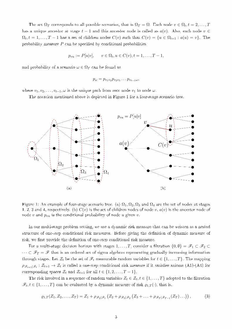
The set ΩT corresponds to all possible scenarios, that is ΩT = Ω. Each node v ∈ Ωt, t = 2, . . . , T
has a unique ancestor at stage t − 1 and this ancestor node is called as a(v). Also, each node v ∈Ωt, t = 1, . . . , T − 1 has a set of children nodes C(v) such that C(v) = u ∈ Ωt+1 : a(u) = v. The
probability measure P can be specied by conditional probabilities
pvu := P [u|v], v ∈ Ωt, u ∈ C(v), t = 1, . . . , T − 1,
and probability of a scenario ω ∈ ΩT can be found as
pω = pv1v2pv2v3 . . . pvt−1ω,
where v1, v2, . . . , vt−1, ω is the unique path from root node v1 to node ω.
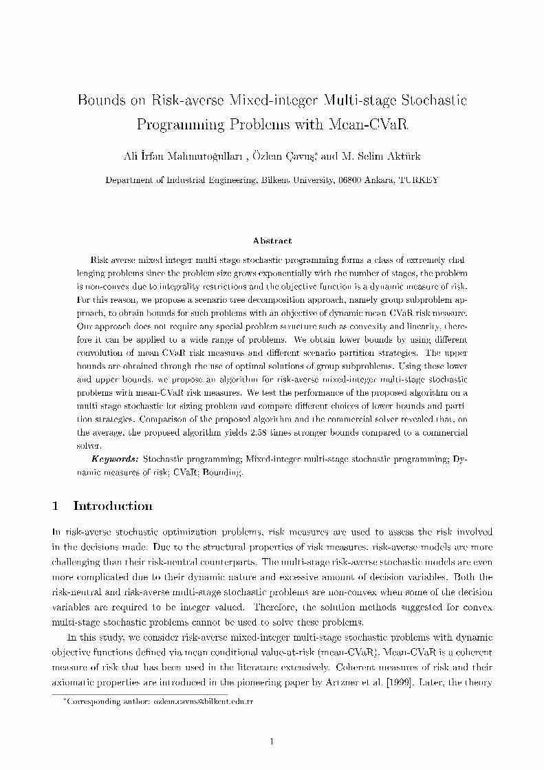
The notation mentioned above is depicted in Figure 1 for a four-stage scenario tree.
(a) (b)
Figure 1: An example of four-stage scenario tree. (a) Ω1,Ω2,Ω3 and Ω4 are the set of nodes at stages1, 2, 3 and 4, respectively. (b) C(v) is the set of children nodes of node v, a(v) is the ancestor node ofnode v and pvu is the conditional probability of node u given v.
In our multi-stage problem setting, we use a dynamic risk measure that can be written as a nested
structure of one-step conditional risk measures. Before giving the denition of dynamic measure of
risk, we rst provide the denition of one-step conditional risk measure.
For a multi-stage decision horizon with stages 1, . . . , T , consider a ltration 0, ∅ = F1 ⊂ F2 ⊂· · · ⊂ FT = F that is an ordered set of sigma algebras representing gradually increasing information
through stages. Let Zt be the set of Ft-measurable random variables for t ∈ 1, . . . , T. The mapping
ρFt+1|Ft: Zt+1 → Zt is called a one-step conditional risk measure if it satises axioms (A1)-(A4) for
corresponding spaces Zt and Zt+1 for all t ∈ 1, 2, . . . , T − 1.The risk involved in a sequence of random variables Zt ∈ Zt, t ∈ 1, . . . , T adopted to the ltration
Ft, t ∈ 1, . . . , T can be evaluated by a dynamic measure of risk %1,T (·), that is,
%1,T (Z1, Z2, . . . , ZT ) = Z1 + ρF2|F1
(Z2 + ρF3|F2
(Z3 + . . .+ ρFT |FT−1
(ZT ) . . .)), (3)
5
where ρFt+1|Ft(·), t ∈ 1, 2, . . . , T − 1 is a one-step conditional risk measure. The structure (3) is
presented in Ruszczynski and Shapiro [2006a]. Later, Ruszczy«ski [2010] shows that the representa-
tion (3) can be constructed using monotonicity of conditional risk measures and the concept of time
consistency.
Collado et al. [2012] show that the dual representation of coherent risk measures can be extended to
dynamic measures of risk. If %1,T (·) is a dynamic risk measure given as in (3), then for every sequence
of random variables Zt ∈ ZtTt=1,
%1,T (Z1, Z2, . . . , ZT ) = maxqT∈QT
〈qT , Z1 + Z2 + · · ·+ ZT 〉, (4)
where
Qt = At−1 · · · A2 A1, (5)
and At = ∂ρFt+1|Ft(0), t ∈ 2, . . . , T. Here 0 ∈ R|Ωt+1|, t ∈ 1, 2, . . . , T − 1 is a vector of all zeros.
QT is a compact and convex set. The operator denes convolution of probability measures, that
is,
(µt qt)(u) = qt(a(u))µt(a(u), u),∀u ∈ Ωt+1,
and
At Qt = µt qt : qt ∈ Qt, µt ∈ At,
for all t ∈ 1, 2, . . . , T − 1. Note that a(u) is the ancestor node of u.
In this study, we use conditional mean-CVaR as one-step conditional risk measure. Therefore, the
next section is devoted to the denition of mean-CVaR.
2.3 CVaR and Mean-CVaR
An important and extensively used example of coherent measures of risk is conditional value-at-Risk
(CVaR). CVaR of Z ∈ Z at level α ∈ [0, 1) is dened as (see [Rockafellar and Uryasev, 2002])
CV aRα(Z) := infη∈R
η +
1
1− αE[(Z − η)+]
, (6)
where (a)+ is positive part of a ∈ R, that is, (a)+ := maxa, 0. The inmum on the right hand side
of (6) holds at V aRα(Z) where V aRα(Z) := infl ∈ R : P (Z ≤ l) ≥ α.Note that, CV aR0(Z) = E[Z] and, CV aRα(Z) converges to the value of Z in the worst case
scenario, i.e. max(Z) = maxi∈1,...,N Zωi , as α ↑ 1. If P is an atomless distribution, CVaR can also
be expressed as:
CV aRα(Z) = E[Z|Z ≥ V aRα(Z)].
In this study, we focus on mean-CVaR, which is a coherent measure of risk. Despite CVaR, mean-
CVaR risk measure conveys the expected value information of a random variable, as well.
Given a weight parameter ε1 ∈ [0, 1] and a level parameter α ∈ [0, 1), mean-CVaR of Z ∈ Z is
dened as
ρ(Z) := (1− ε1)E[Z] + ε1CV aRα(Z). (7)
As seen in (7), mean-CVaR is a convex combination of expected value of a given random variable Z
and CVaR value of this random variable at level α. As ε1 or α increase, ρ(·) gets more risk averse. If
6
ε1 = 0, then ρ(Z) = E[Z], similarly ρ(Z) = CV aRα(Z) when ε1 = 1.
The expression in (7) can equivalently be represented as following linear program for nite proba-
bility spaces.
ρ(Z) = minimize (1− ε1)∑ω∈Ω
pωZω + ε1
(η +
1
1− α∑ω∈Ω
pωϑω
),
subject to ϑω ≥ Zω − η, ∀ω ∈ Ω,
η urs, ϑω ≥ 0, ∀ω ∈ Ω.
When the sample space is nite, the dual representation (2) holds for mean-CVaR with the set Arepresented as (see [Ruszczynski and Shapiro, 2006b]):
A =µ ∈ RN : 1− ε1 ≤ µω ≤ 1 + ε2, ∀ω ∈ Ω and E[µ] = 1
, (8)
where
ε2 :=α
1− αε1 ≥ 0.
Similarly, for any Z ∈ Zt+1, the one-step conditional mean-CVaR risk measure ρFt+1|Ft(Z) with
parameters εt1 ∈ [0, 1] and αt ∈ [0, 1) is dened as:
ρFt+1|Ft(Z) := (1− εt1)E[Z|Ft] + εt1 inf
η∈Zt
η +
1
1− αtE[(Z − η)+|Ft]
. (9)
Its dual set At, t ∈ 1, 2, . . . , T − 1 is
At =µt ∈ R|Ωt+1| : 1− εt1 ≤ µtω ≤ 1 + εt2, ∀ω ∈ Ωt+1 and E[µt|Ft] = 1
, (10)
where εt2 = (αt/(1− αt))εt1 and 1 ∈ R|Ωt|.
Due to the one-to-one correspondence between a risk measure and its dual set, a mean-CVaR
risk measure can either be dened as in (7) with parameters ε1 and α, or via its dual as in (8) with
parameters ε1 and ε2.
3 Bounds
The main motivation of this section is to propose lower and upper bounds for problem (1) with an
objective of dynamic mean-CVaR. Therefore, using scenario groups, we rst propose a continuum of
lower bounds for mean-CVaR risk measure. Some possible lower bounds are presented in Section 3.2.
The application of these bounds to a risk-averse mixed-integer multi-stage stochastic problems with an
objective of (3) is presented in Section 3.3. Extension of the proposed lower bounds to other dynamic
mean-CVaR risk measures is discussed in Section 3.4. In Section 3.5, we propose a method for obtaining
an upper bound to the problem. The proposed algorithm benets these results and yields lower and
upper bounds for the problem.
3.1 Lower Bounds for Mean-CVaR Risk Measure
Let ρ(·) and ρ(·) be two coherent measures of risk with dual sets A and A, respectively. In Proposition
1, we derive the necessary condition that ρ(·) gives a lower bound for ρ(·).
7
Proposition 1: ρ(Z) ≤ ρ(Z) for all Z ∈ Z if A ⊆ A.Proof: For any Z ∈ Z, let µ∗ ∈ A such that maximization in equation (2) is attained at µ∗ for
ρ(Z), that is, ρ(Z) = 〈µ∗, Z〉. If A ⊆ A, then µ∗ ∈ A and 〈µ∗, Z〉 ≤ maxµ∈A〈µ,Z〉 = ρ(Z). Since Z is
arbitrary, desired inequality follows.
Although a similar version of Proposition 1 is presented in Iancu et al. [2015], our purpose is to
derive lower bounds for risk averse problems with an objective of dynamic mean-CVaR risk measure
by using Proposition 1. Hence, we try to construct a risk measure ρ(·), or equivalently its dual set A,in such a way that both computation of lower bound is easy and obtained lower bound is tight.
The risk measure ρ(·), or equivalently its dual set A, can be constructed in dierent ways. When
the cardinality of the sample space is large, due to computational concerns, one may think of dealing
with subsets of sample space separately and then obtain a lower bound information for ρ(·). For suchconstruction, we need the denition of scenario groups and partition. A subset of scenarios S ⊆ Ω
is called as a group. Let S = SjJj=1 be a collection of groups that forms a partition of Ω, that is,⋃Jj=1 Sj = Ω and Sj
⋂Sj′ = ∅ for all j, j′ ∈ 1, 2, . . . , J such that j 6= j′. Note that the groups may
not be necessarily disjoint (see [Sandkç and Özaltn, 2014]), i.e. Sj⋂Sj′ 6= ∅, but for the ease of
representation, we partition the sample space into disjoint groups. Let G be a σ−algebra generated
by partition S where each group Sj ∈ S corresponds to an elementary event of G . The probability of
an elementary event corresponding to Sj is pj =∑
ω∈Sjpω which is the total probability of scenarios
in Sj . We also dene the adjusted probability of each scenario ω as pjω = pω/pj for all ω ∈ Sj andj ∈ 1, 2, . . . , J. Note that, G is a sub σ−algebra of F .
Once a partition of sample space is given, one way to construct ρ(·) is to dene it as a convolutionof a coherent risk measure ρG : G → R and a one-step conditional risk measure ρF |G : F → G , that
is, ρ(·) = (ρG ρF |G )(·), or equivalently, dene its dual set as a convolution of sets AG and AF |G such
that A = AF |G AG .
The one-step conditional risk measure ρF |G (·) is dened by conditioning to each elementary event
of G . Let ρSj : σ(Sj)→ R be a coherent risk measure for the elementary event j of G . Then, ρF |G (·)can be represented in terms of ρSj (·), j ∈ 1, 2 . . . , J, that is,
[ρF |G (·)
]j
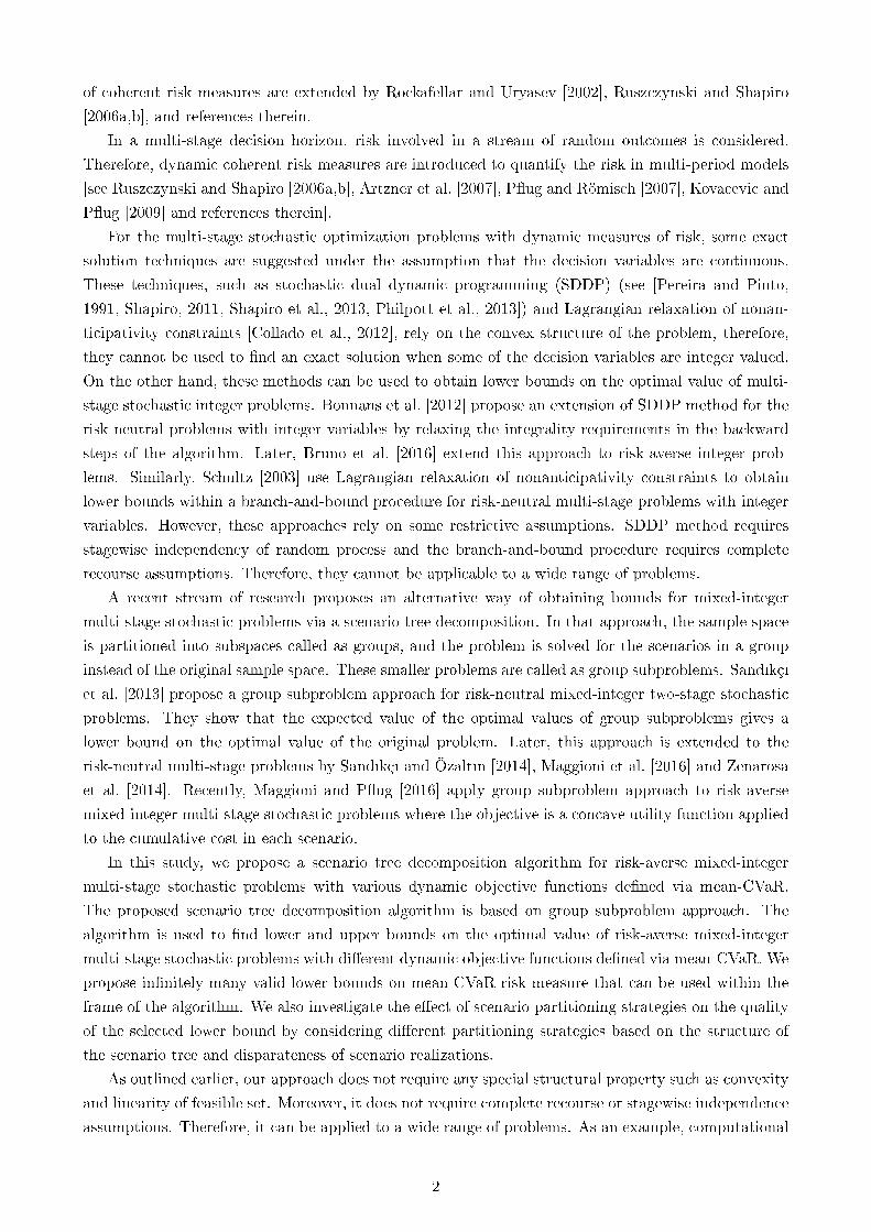
= ρSj (·). Figure 2 depicts
aforementioned notation for a given partition of scenario tree with ve scenarios.
For the remainder of the paper, we will focus on mean-CVaR risk measure. Hence, we will use ρ(·)to refer a mean-CVaR risk measure as in (7) and ρFt+1|Ft
(·), t ∈ 1, 2 . . . , T − 1 to refer a one-step
conditional mean-CVaR risk measure as in (9).
For mean-CVaR case, ρ(·) or equivalently its dual set A, can be explicitly stated. Let parameters of
ρG be ε11 ∈ [0, 1] and ε12 ≥ 0, and parameters of ρF |G be ε21 ∈ [0, 1] and ε22 ≥ 0. Consider the convolution
ρ = ρG ρF |G : F → R and its dual set
A = AF |G AG = µ ∈ RN : µ = µ1 µ2, µ1 ∈ AG , µ2 ∈ AF |G
= µ ∈ RN : µ = µ1 µ2, 1− ε11 ≤ µ1j ≤ 1 + ε12, ∀j ∈ 1, 2 . . . , J and E[µ1] = 1,
1− ε21 ≤ µ2ω ≤ 1 + ε22,∀ω ∈ Ω and E[µ2|G ] = 1, (11)
where 1 ∈ RJ . Construction of the set A for the example in Figure 2 can be seen in Appendix A.
Now, we are ready to prove that a lower bound for mean-CVaR risk measure ρ(·) can be obtained
by convolution of AG (·) and AF |G (·).Proposition 2: Let ρ(·) be mean-CVaR risk measure with dual set A and ρ(·) be dened with
8
(a) (b)
(c) (d)
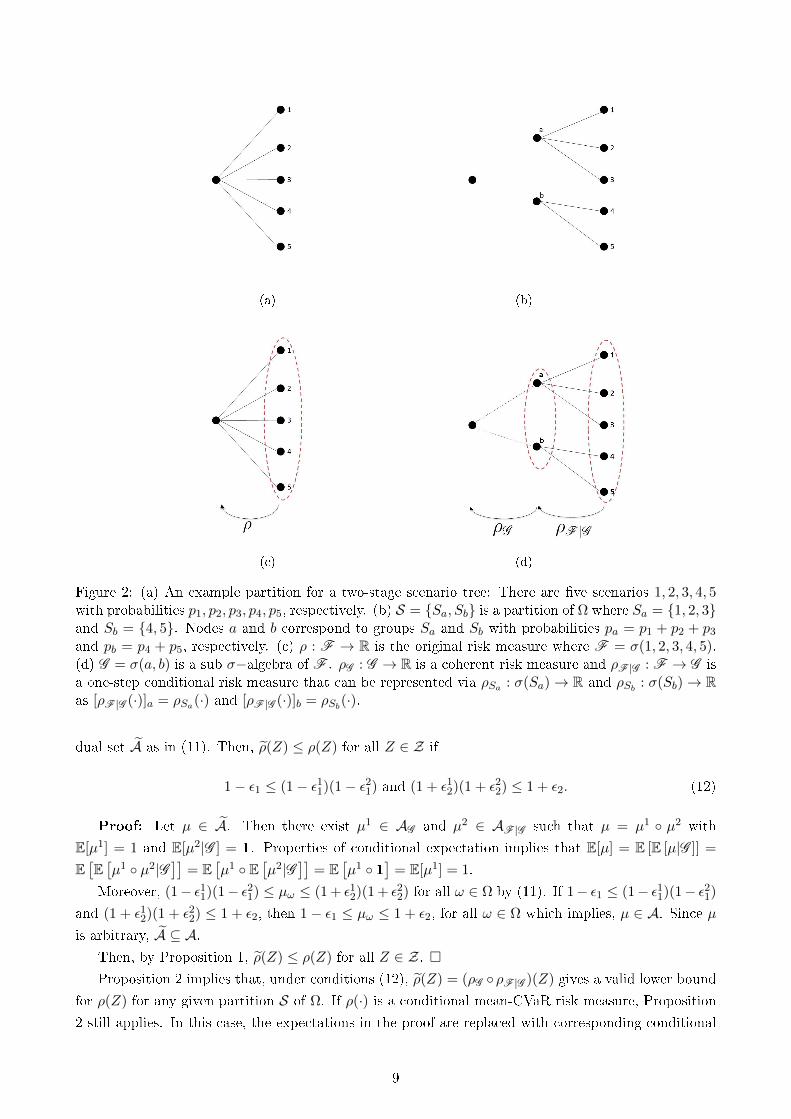
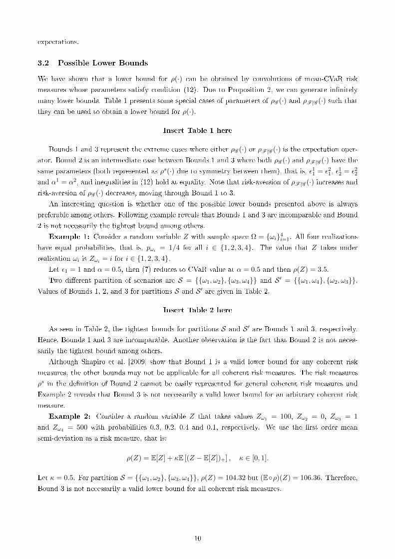
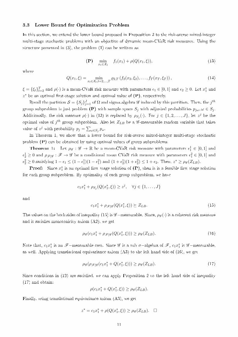
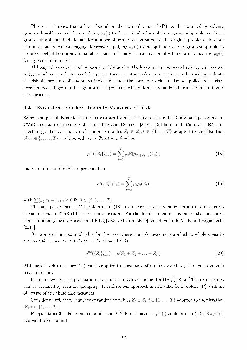
Figure 2: (a) An example partition for a two-stage scenario tree: There are ve scenarios 1, 2, 3, 4, 5with probabilities p1, p2, p3, p4, p5, respectively. (b) S = Sa, Sb is a partition of Ω where Sa = 1, 2, 3and Sb = 4, 5. Nodes a and b correspond to groups Sa and Sb with probabilities pa = p1 + p2 + p3
and pb = p4 + p5, respectively. (c) ρ : F → R is the original risk measure where F = σ(1, 2, 3, 4, 5).(d) G = σ(a, b) is a sub σ−algebra of F . ρG : G → R is a coherent risk measure and ρF |G : F → G isa one-step conditional risk measure that can be represented via ρSa : σ(Sa)→ R and ρSb
: σ(Sb)→ Ras [ρF |G (·)]a = ρSa(·) and [ρF |G (·)]b = ρSb
(·).
dual set A as in (11). Then, ρ(Z) ≤ ρ(Z) for all Z ∈ Z if
1− ε1 ≤ (1− ε11)(1− ε21) and (1 + ε12)(1 + ε22) ≤ 1 + ε2. (12)
Proof: Let µ ∈ A. Then there exist µ1 ∈ AG and µ2 ∈ AF |G such that µ = µ1 µ2 with
E[µ1] = 1 and E[µ2|G ] = 1. Properties of conditional expectation implies that E[µ] = E [E [µ|G ]] =
E[E[µ1 µ2|G
]]= E
[µ1 E
[µ2|G
]]= E
[µ1 1
]= E[µ1] = 1.
Moreover, (1− ε11)(1− ε21) ≤ µω ≤ (1 + ε12)(1 + ε22) for all ω ∈ Ω by (11). If 1− ε1 ≤ (1− ε11)(1− ε21)
and (1 + ε12)(1 + ε22) ≤ 1 + ε2, then 1− ε1 ≤ µω ≤ 1 + ε2, for all ω ∈ Ω which implies, µ ∈ A. Since µis arbitrary, A ⊆ A.
Then, by Proposition 1, ρ(Z) ≤ ρ(Z) for all Z ∈ Z. Proposition 2 implies that, under conditions (12), ρ(Z) = (ρG ρF |G )(Z) gives a valid lower bound
for ρ(Z) for any given partition S of Ω. If ρ(·) is a conditional mean-CVaR risk measure, Proposition
2 still applies. In this case, the expectations in the proof are replaced with corresponding conditional
9
expectations.
3.2 Possible Lower Bounds
We have shown that a lower bound for ρ(·) can be obtained by convolutions of mean-CVaR risk
measures whose parameters satisfy condition (12). Due to Proposition 2, we can generate innitely
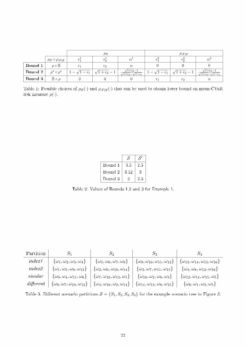
many lower bounds. Table 1 presents some special cases of parameters of ρG (·) and ρF |G (·) such that
they can be used to obtain a lower bound for ρ(·).
Insert Table 1 here
Bounds 1 and 3 represent the extreme cases where either ρG (·) or ρF |G (·) is the expectation oper-
ator. Bound 2 is an intermediate case between Bounds 1 and 3 where both ρG (·) and ρF |G (·) have thesame parameters (both represented as ρs(·) due to symmetry between them), that is, ε11 = ε21, ε
12 = ε22
and α1 = α2, and inequalities in (12) hold at equality. Note that risk-aversion of ρF |G (·) increases andrisk-aversion of ρG (·) decreases, moving through Bound 1 to 3.
An interesting question is whether one of the possible lower bounds presented above is always
preferable among others. Following example reveals that Bounds 1 and 3 are incomparable and Bound
2 is not necessarily the tightest bound among others.
Example 1: Consider a random variable Z with sample space Ω = ωi4i=1. All four realizations
have equal probabilities, that is, pωi = 1/4 for all i ∈ 1, 2, 3, 4. The value that Z takes under
realization ωi is Zωi = i for i ∈ 1, 2, 3, 4.Let ε1 = 1 and α = 0.5, then (7) reduces to CVaR value at α = 0.5 and then ρ(Z) = 3.5.
Two dierent partition of scenarios are S = ω1, ω2, ω3, ω4 and S ′ = ω1, ω4, ω2, ω3.Values of Bounds 1, 2, and 3 for partitions S and S ′ are given in Table 2.
Insert Table 2 here
As seen in Table 2, the tightest bounds for partitions S and S ′ are Bounds 1 and 3, respectively.
Hence, Bounds 1 and 3 are incomparable. Another observation is the fact that Bound 2 is not neces-
sarily the tightest bound among others.
Although Shapiro et al. [2009] show that Bound 1 is a valid lower bound for any coherent risk
measures, the other bounds may not be applicable for all coherent risk measures. The risk measures
ρs in the denition of Bound 2 cannot be easily represented for general coherent risk measures and
Example 2 reveals that Bound 3 is not necessarily a valid lower bound for an arbitrary coherent risk
measure.
Example 2: Consider a random variable Z that takes values Zω1 = 100, Zω2 = 0, Zω3 = 1
and Zω4 = 500 with probabilities 0.3, 0.2, 0.4 and 0.1, respectively. We use the rst order mean
semi-deviation as a risk measure, that is:
ρ(Z) = E[Z] + κE [(Z − E[Z])+] , κ ∈ [0, 1].
Let κ = 0.5. For partition S = ω1, ω2, ω3, ω4, ρ(Z) = 104.32 but (Eρ)(Z) = 106.36. Therefore,
Bound 3 is not necessarily a valid lower bound for all coherent risk measures.
10
3.3 Lower Bound for Optimization Problem
In this section, we extend the lower bound proposed in Proposition 2 to the risk-averse mixed-integer
multi-stage stochastic problems with an objective of dynamic mean-CVaR risk measures. Using the
structure presented in (3), the problem (1) can be written as
(P) minx1∈X1
f1(x1) + ρ(Q(x1, ξ)), (13)
where
Q(x1, ξ) = minxt∈Xt,t=2,...,T
%2,T (f2(x2, ξ2), . . . , fT (xT , ξT )) , (14)
ξ = ξtTt=2 and ρ(·) is a mean-CVaR risk measure with parameters ε1 ∈ [0, 1] and ε2 ≥ 0. Let x∗1 and
z∗ be an optimal rst-stage solution and optimal value of (P), respectively.
Recall the partition S = SjJj=1 of Ω and sigma algebra G induced by this partition. Then, the jth
group subproblem is just problem (P) with sample space Sj with adjusted probabilities pjω, ω ∈ Sj .Additionally, the risk measure ρ(·) in (13) is replaced by ρSj (·). For j ∈ 1, 2, . . . , J, let zj be the
optimal value of jth group subproblem. Also let ZLB be a G -measurable random variable that takes
value of zj with probability pj =∑
ω∈Sjpω.
In Theorem 1, we show that a lower bound for risk-averse mixed-integer multi-stage stochastic
problem (P) can be obtained by using optimal values of group subproblems.
Theorem 1: Let ρG : G → R be a mean-CVaR risk measure with parameters ε11 ∈ [0, 1] and
ε12 ≥ 0 and ρF |G : F → G be a conditional mean-CVaR risk measure with parameters ε21 ∈ [0, 1] and
ε22 ≥ 0 satisfying 1− ε1 ≤ (1− ε11)(1− ε21) and (1 + ε12)(1 + ε22) ≤ 1 + ε2. Then, z∗ ≥ ρG (ZLB).
Proof: Since x∗1 is an optimal rst stage solution of (P), then it is a feasible rst stage solution
for each group subproblem. By optimality of each group subproblem, we have
c1x∗1 + ρSj (Q(x∗1, ξ)) ≥ zj , ∀j ∈ 1, . . . , J
and
c1x∗1 + ρF |G (Q(x∗1, ξ)) ZLB. (15)
The values on the both sides of inequality (15) is G−measurable. Since, ρG (·) is a coherent risk measure
and it satises monotonicity axiom (A2), we get
ρG (c1x∗1 + ρF |G (Q(x∗1, ξ))) ≥ ρG (ZLB). (16)
Note that, c1x∗1 is an F−measurable cost. Since G is a sub σ−algebra of F , c1x
∗1 is G−measurable,
as well. Applying translational equivariance axiom (A3) to the left hand side of (16), we get
ρG (ρF |G (c1x∗1 +Q(x∗1, ξ))) ≥ ρG (ZLB). (17)
Since conditions in (12) are satised, we can apply Proposition 2 to the left hand side of inequality
(17) and obtain:
ρ(c1x∗1 +Q(x∗1, ξ)) ≥ ρG (ZLB).
Finally, using translational equivariance axiom (A3), we get
z∗ = c1x∗1 + ρ(Q(x∗1, ξ)) ≥ ρG (ZLB).
11
Theorem 1 implies that a lower bound on the optimal value of (P) can be obtained by solving
group subproblems and then applying ρG (·) to the optimal values of these group subproblems. Since
group subproblems include smaller number of scenarios compared to the original problem, they are
computationally less challenging. Moreover, applying ρG (·) to the optimal values of group subproblems
requires negligible computational eort, since it is only the calculation of value of a risk measure ρG (·)for a given random cost.
Although the dynamic risk measure widely used in the literature is the nested structure presented
in (3), which is also the focus of this paper, there are other risk measures that can be used to evaluate
the risk of a sequence of random variables. We show that our approach can also be applied to the risk-
averse mixed-integer multi-stage stochastic problems with dierent dynamic extensions of mean-CVaR
risk measure.
3.4 Extension to Other Dynamic Measures of Risk
Some examples of dynamic risk measures apart from the nested structure in (3) are multiperiod mean-
CVaR and sum of mean-CVaR (see Pug and Römisch [2007], Eichhorn and Römisch [2005], re-
spectively). For a sequence of random variables Zt ∈ Zt, t ∈ 1, . . . , T adopted to the ltration
Ft, t ∈ 1, . . . , T, multiperiod mean-CVaR is dened as
ρm(ZtTt=2) =
T∑t=2
µtE[ρFt|Ft−1(Zt)], (18)
and sum of mean-CVaR is represented as
ρs(ZtTt=2) =T∑t=2
µtρt(Zt), (19)
with∑T
t=2 µt = 1, µt ≥ 0 for t ∈ 2, 3, . . . , T.The multiperiod mean-CVaR risk measure (18) is a time consistent dynamic measure of risk whereas
the sum of mean-CVaR (19) is not time consistent. For the denition and discussion on the concept of
time consistency, see Kovacevic and Pug [2009], Shapiro [2009] and Homem-de Mello and Pagnoncelli
[2016].
Our approach is also applicable for the case where the risk measure is applied to whole scenario
cost as a time inconsistent objective function, that is,
ρnd(ZtTt=1) = ρ(Z1 + Z2 + . . .+ ZT ). (20)
Although the risk measure (20) can be applied to a sequence of random variables, it is not a dynamic
measure of risk.
In the following three propositions, we show that a lower bound for (18), (19) or (20) risk measures
can be obtained by scenario grouping. Therefore, our approach is still valid for Problem (P) with an
objective of one these risk measures.
Consider an arbitrary sequence of random variables Zt ∈ Zt, t ∈ 1, . . . , T adopted to the ltrationFt, t ∈ 1, . . . , T.
Proposition 3: For a multiperiod mean-CVaR risk measure ρm(·) as dened in (18), E ρm(·)is a valid lower bound.
12
Proof: If multiperiod mean-CVaR risk measure (18) is applied to the sequence Zt ∈ Zt, t ∈1, . . . , T, then
ρm(ZtTt=2) =T∑t=2
µtE[ρFt|Ft−1
(Zt)].
Since ρFt|Ft−1(·) is a conditional mean-CVaR risk measure, the lower bound E ρFt|Ft−1
(·) applies fort ∈ 2, 3, . . . , T. Then,
ρm(ZtTt=2) ≥T∑t=2
µtE[E[ρFt|Ft−1
(Zt)]].
To avoid notational ambiguity, expectation operators are given without reference sigma algebras. Since
expectation is a linear operator, we get
ρm(ZtTt=2) ≥ E
[T∑t=2
µtE[ρFt|Ft−1(Zt)]
],
or equivalently,
ρm(ZtTt=2) ≥ E[ρm(ZtTt=2)
].
Since the sequence Zt ∈ Zt, t ∈ 1, . . . , T is arbitrary, the desired result follows.
Proposition 4: For a sum of mean-CVaR risk measure ρs(·) as dened in (19), E ρm(·) is a
valid lower bound.
Proof: If sum of mean-CVaR risk measure (19) is applied to the sequence Zt ∈ Zt, t ∈ 1, . . . , T,then
ρs(ZtTt=2) =
T∑t=2
µtρt(Zt).
Similarly, E ρt(·) applies for t ∈ 2, 3, . . . , T. Then,
ρs(ZtTt=2) ≥T∑t=2
µtE [ρt(Zt)] ,
and
ρs(ZtTt=2) ≥ E
[T∑t=2
µtρt(Zt)
],
or equivalently,
ρs(ZtTt=2) ≥ E[ρs(ZtTt=2)
].
Since the sequence Zt ∈ Zt, t ∈ 1, . . . , T is arbitrary, the desired result follows.
Proposition 5: For the risk measure ρnd(·) as dened in (20), ρG ρF |G (·) is a valid lower bound
if parameters of ρG (·) and ρF |G (·) satisfy conditions in (12).
Proof: If the mean-CVaR risk measure (20) is applied to the sequence Zt ∈ Zt, t ∈ 1, . . . , T,then
ρnd(ZtTt=1) = ρ(Z1 + Z2 + . . .+ ZT ).
Since ρG (·) and ρF |G (·) satisfy conditions in (12), their convolution is a valid lower bound on mean-
CVaR risk measure ρ(·), that is,
ρnd(ZtTt=1) ≥ ρG ρF |G (Z1 + Z2 + . . .+ ZT ),
13
or equivalently,
ρnd(ZtTt=1) = ρG ρF |G (ZtTt=1).
Since the sequence Zt ∈ Zt, t ∈ 1, . . . , T is arbitrary, the desired result follows.
As shown above, our proposed lower bound is quite general and can be applied to other dynamic
mean-CVaR measures.
3.5 Upper Bound for Optimization Problem
Obtaining an upper bound, or equivalently nding a feasible solution of a minimization problem, is
crucial for the instances where an optimal solution is not available. A good quality feasible solution
gives the decision maker an action to be taken and measures the quality of obtained lower bound when
an optimal solution is not available.
An upper bound for the optimal value of (P) can be obtained by using optimal solutions of group
subproblems. Once jth group subproblem is solved, an optimal solution of it, namely xj , is obtained.
Let UBj be the optimal value of (P) where (some of) the variables appearing in jth group subproblem
are set to xj . We call this problem as restricted problem. Since some of the problem variables are
xed, solving the restricted problem is easier than the original one and the resulting scenario tree can
become decomposable.
If xj is not feasible for original problem (P), then corresponding upper bound UBj is set to
innity. The best available upper bound UB is obtained by taking minimum of UBj values over all
j ∈ 1, . . . , J, that is,
UB = minj∈1,...,J
UBj . (21)
In Algorithm 1, we present how group subproblem approach can be used to obtain lower and upper
bounds for a multi-stage risk-averse mixed-integer problem with mean-CVaR objective.
4 Computational Experiments
In this section, we conduct our numerical experiments on a multi-stage lot sizing problem studied in
Guan et al. [2009]. All computational experiments are performed on an Intel(R) Core(TM) i7-4790
[email protected] GHz computer with 8.00 GB of RAM with Java 1.8.0.31 and IBM ILOG CPLEX 12.6. We
rst introduce risk-averse multi-stage lot sizing problem (RAMLSP) with mean-CVaR risk measure.
Then, we compare the results obtained via usage of dierent scenario partition strategies and lower
bound choices. We also compare the proposed algorithm and CPLEX in terms of solution quality and
required CPU time.
4.1 Risk-averse Multi-stage Lot Sizing Problem with Mean-CVaR
The objective of RAMLSP is to minimize the dynamic risk measure over T periods dened via mean-
CVaR risk measures subject to demand satisfaction and capacity constraints. RAMLSP-T-r represents
a RAMLSP instance with T stages in which random components can take r dierent values at each
stage. Therefore, total number of scenarios in an RAMLSP-T-r instance is rT−1. We generate random
test instances as in Guan et al. [2009]. The same setting of the parameters is also used by Sandkç and
14
Algorithm 1 Lower and upper bounds for (P)
Input: A risk-averse mixed-integer multi-stage stochastic problem (P) and a partition S = SjJj=1
of sample space Ω.Initialize: LB ← −∞ and UB ← +∞
Lower Bounding:
for all j ∈ 1, 2, . . . , J doSolve the jth group subproblem.xj ← an optimal solution of jth group subproblemzj ← optimal value of jth group subproblem
end for
Let ZLB be a random variable that takes value zj with probability pj =∑
ω∈Sjpω
LB ← ρG (ZLB)
Upper Bounding:
for all j ∈ 1, 2, . . . , J doUBj ← the optimal value of the original problem with the additional constraint where (some of)the variables appearing in jth group subproblem are set to xj .
end for
UB ← minj∈1,2...,J UBj
Return: LB and UB
Özaltn [2014], that is, htu ∼ U [0, 10], αtu ∼ U [3.2, 4.8]E[h], βtu ∼ U [320, 480]E[h], dtu ∼ U [0, 100]
and Mtu ∼ U [40T, 60T ], where U [a, b] represents discrete uniform distribution between a and b.
Using the scenario tree representation given in Section 2.2, RAMLSP can be stated as follows:
(RAMLSP) minimize Z1 + ρF2|F1
(Z2 + ρF3|F2
(Z3 + . . .+ ρFT |FT−1
(ZT ) . . .)), (22)
subject to Ztu = αtuxtu + βtuytu + htustu, ∀t = 1, . . . , T and u ∈ Ωt, (23)
s(t−1)a(u) + xtu = dtu + stu, ∀t = 1, . . . , T and u ∈ Ωt, (24)
xtu ≤Mtuytu, ∀t = 1, . . . , T and u ∈ Ωt, (25)
xtu, stu ≥ 0 and integer, ytu ∈ 0, 1 ∀t = 1, . . . , T and u ∈ Ωt, (26)
sa(v1) = 0.
Here xtu is the production level, ytu is the setup indicator and stu is the inventory level variables at
node u ∈ Ωt in period t = 1, . . . , T . αtu, βtu, htu, dtu and Mtu denote unit production cost, setup cost,
inventory holding cost, demand and production capacity parameters, respectively. Z1 is the total of
deterministic production, setup and inventory holding costs incurred in the rst stage. Similarly, Ztuis the cost incurred at node u ∈ Ωt at stage t = 2, . . . , T . Zt represents the random variable that takes
values of Ztu, u ∈ Ωt with respective probabilities. The objective (22) is the dynamic risk value over
the planning horizon. Constraints (23) calculate the cost incurred at each node of the scenario tree.
Constraints (24) and (25) are inventory balance and capacity constraints. Constraints (26) are domain
constraints. Unlike Guan et al. [2009] and Sandkç and Özaltn [2014], we assume that production
and inventory levels are required to be integer valued. Although this assumption increases the problem
complexity, we have a more realistic representation to evaluate the performance of the algorithm.
15
For the computational experiments, we use three dierent values of weight parameter ε1 ∈ 0.8, 0.5, 0.3and level parameter α ∈ 0.9, 0.8, 0.7 of mean-CVaR. Therefore, we have nine dierent risk aversion
settings.
4.2 Choices of Scenario Partitions and Lower Bounds
As seen in Example 1, the value of each lower bound highly depends on chosen scenario partition. We
consider four possible scenario partitions obtained by dierent scenario grouping strategies, namely
index1, index2, similar and dierent. Partitions index1 and index2 are based on scenario tree structure.
In partition index1, the last stage nodes sharing the same ancestor node are placed in the same group.
On the other hand, index2 is obtained by placing the last stage nodes with dierent ancestor nodes in
the same group.
If a priori information on the cost of each single scenario under the optimal solution is available,
the groups can also be obtained with respect to similarity and diversity of individual scenarios. How-
ever, this information is not available before solving the original problem. Therefore, the deterministic
version of the original problem can be solved for each scenario separately, and these optimal values
can be used to approximate the cost of each scenario under an optimal solution of original problem. In
partition similar, the partition is obtained by placing the scenarios with close approximate costs in a
group. On the other hand, partition dierent is obtained by placing the scenarios with distant approx-
imate costs in a group. Note that, for partitions similar and dierent, an additional computational
eort is required to obtain approximate costs.
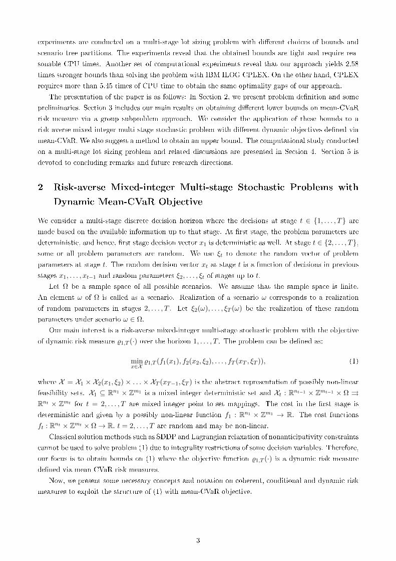
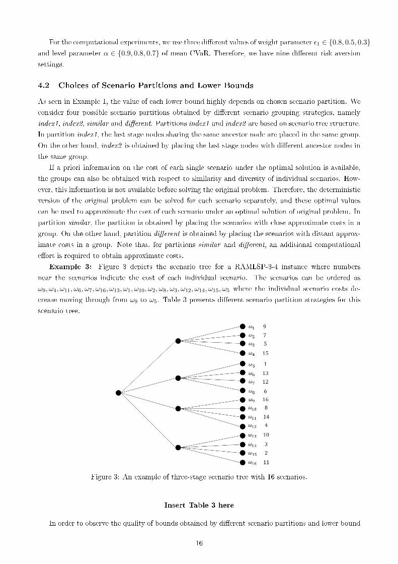
Example 3: Figure 3 depicts the scenario tree for a RAMLSP-3-4 instance where numbers
near the scenarios indicate the cost of each individual scenario. The scenarios can be ordered as
ω9, ω4, ω11, ω6, ω7, ω16, ω13, ω1, ω10, ω2, ω8, ω3, ω12, ω14, ω15, ω5 where the individual scenario costs de-
crease moving through from ω9 to ω5. Table 3 presents dierent scenario partition strategies for this
scenario tree.
Figure 3: An example of three-stage scenario tree with 16 scenarios.
Insert Table 3 here
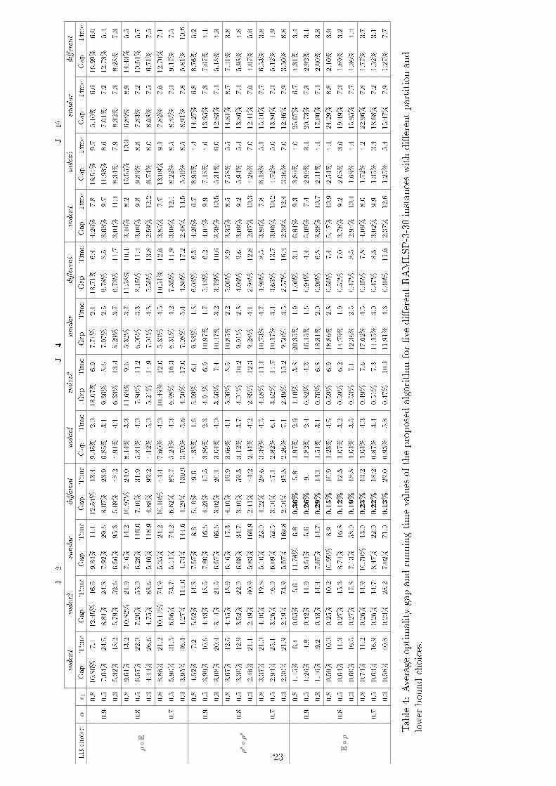
In order to observe the quality of bounds obtained by dierent scenario partitions and lower bound
16
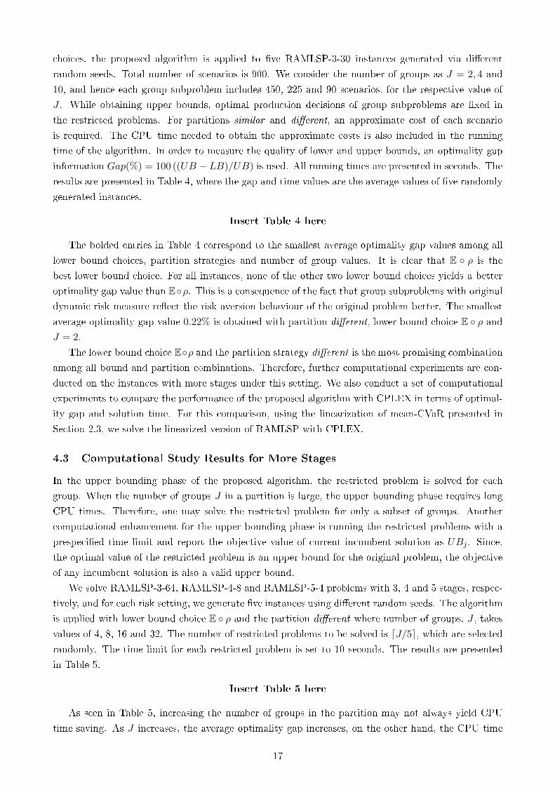
choices, the proposed algorithm is applied to ve RAMLSP-3-30 instances generated via dierent
random seeds. Total number of scenarios is 900. We consider the number of groups as J = 2, 4 and
10, and hence each group subproblem includes 450, 225 and 90 scenarios, for the respective value of
J . While obtaining upper bounds, optimal production decisions of group subproblems are xed in
the restricted problems. For partitions similar and dierent, an approximate cost of each scenario
is required. The CPU time needed to obtain the approximate costs is also included in the running
time of the algorithm. In order to measure the quality of lower and upper bounds, an optimality gap
information Gap(%) = 100 ((UB − LB)/UB) is used. All running times are presented in seconds. The
results are presented in Table 4, where the gap and time values are the average values of ve randomly
generated instances.
Insert Table 4 here
The bolded entries in Table 4 correspond to the smallest average optimality gap values among all
lower bound choices, partition strategies and number of group values. It is clear that E ρ is the
best lower bound choice. For all instances, none of the other two lower bound choices yields a better
optimality gap value than Eρ. This is a consequence of the fact that group subproblems with original
dynamic risk measure reect the risk aversion behaviour of the original problem better. The smallest
average optimality gap value 0.22% is obtained with partition dierent, lower bound choice E ρ and
J = 2.
The lower bound choice Eρ and the partition strategy dierent is the most promising combination
among all bound and partition combinations. Therefore, further computational experiments are con-
ducted on the instances with more stages under this setting. We also conduct a set of computational
experiments to compare the performance of the proposed algorithm with CPLEX in terms of optimal-
ity gap and solution time. For this comparison, using the linearization of mean-CVaR presented in
Section 2.3, we solve the linearized version of RAMLSP with CPLEX.
4.3 Computational Study Results for More Stages
In the upper bounding phase of the proposed algorithm, the restricted problem is solved for each
group. When the number of groups J in a partition is large, the upper bounding phase requires long
CPU times. Therefore, one may solve the restricted problem for only a subset of groups. Another
computational enhancement for the upper bounding phase is running the restricted problems with a
prespecied time limit and report the objective value of current incumbent solution as UBj . Since,
the optimal value of the restricted problem is an upper bound for the original problem, the objective
of any incumbent solution is also a valid upper bound.
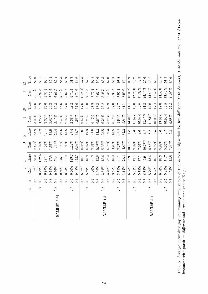
We solve RAMLSP-3-64, RAMLSP-4-8 and RAMLSP-5-4 problems with 3, 4 and 5 stages, respec-
tively, and for each risk setting, we generate ve instances using dierent random seeds. The algorithm
is applied with lower bound choice E ρ and the partition dierent where number of groups, J , takes
values of 4, 8, 16 and 32. The number of restricted problems to be solved is dJ/5e, which are selected
randomly. The time limit for each restricted problem is set to 10 seconds. The results are presented
in Table 5.
Insert Table 5 here
As seen in Table 5, increasing the number of groups in the partition may not always yield CPU
time saving. As J increases, the average optimality gap increases, on the other hand, the CPU time
17
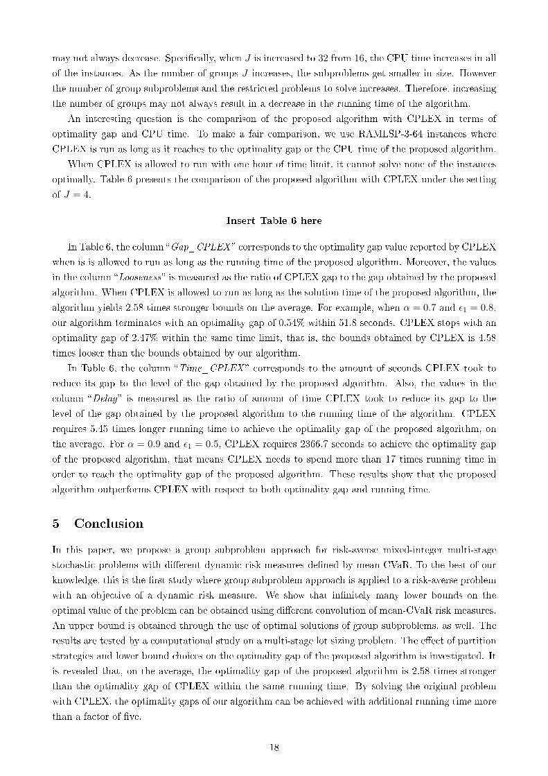
may not always decrease. Specically, when J is increased to 32 from 16, the CPU time increases in all
of the instances. As the number of groups J increases, the subproblems get smaller in size. However
the number of group subproblems and the restricted problems to solve increases. Therefore, increasing
the number of groups may not always result in a decrease in the running time of the algorithm.
An interesting question is the comparison of the proposed algorithm with CPLEX in terms of
optimality gap and CPU time. To make a fair comparison, we use RAMLSP-3-64 instances where
CPLEX is run as long as it reaches to the optimality gap or the CPU time of the proposed algorithm.
When CPLEX is allowed to run with one hour of time limit, it cannot solve none of the instances
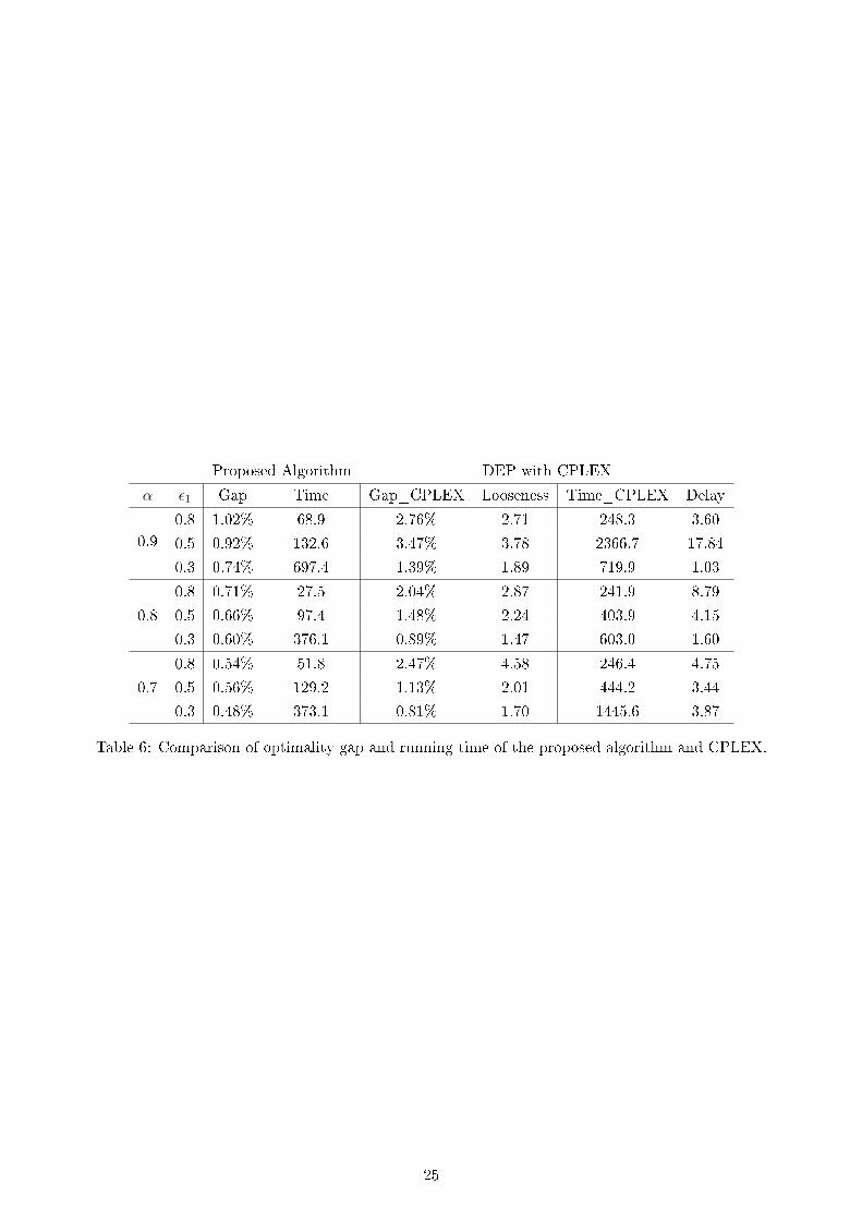
optimally. Table 6 presents the comparison of the proposed algorithm with CPLEX under the setting
of J = 4.
Insert Table 6 here
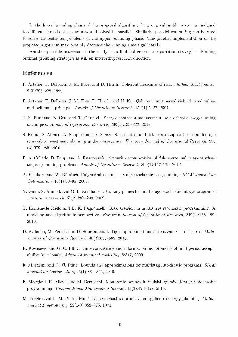
In Table 6, the column Gap_CPLEX corresponds to the optimality gap value reported by CPLEX
when is is allowed to run as long as the running time of the proposed algorithm. Moreover, the values
in the column Looseness is measured as the ratio of CPLEX gap to the gap obtained by the proposed
algorithm. When CPLEX is allowed to run as long as the solution time of the proposed algorithm, the
algorithm yields 2.58 times stronger bounds on the average. For example, when α = 0.7 and ε1 = 0.8,
our algorithm terminates with an optimality gap of 0.54% within 51.8 seconds. CPLEX stops with an
optimality gap of 2.47% within the same time limit, that is, the bounds obtained by CPLEX is 4.58
times looser than the bounds obtained by our algorithm.
In Table 6, the column Time_CPLEX corresponds to the amount of seconds CPLEX took to
reduce its gap to the level of the gap obtained by the proposed algorithm. Also, the values in the
column Delay is measured as the ratio of amount of time CPLEX took to reduce its gap to the
level of the gap obtained by the proposed algorithm to the running time of the algorithm. CPLEX
requires 5.45 times longer running time to achieve the optimality gap of the proposed algorithm, on
the average. For α = 0.9 and ε1 = 0.5, CPLEX requires 2366.7 seconds to achieve the optimality gap
of the proposed algorithm, that means CPLEX needs to spend more than 17 times running time in
order to reach the optimality gap of the proposed algorithm. These results show that the proposed
algorithm outperforms CPLEX with respect to both optimality gap and running time.
5 Conclusion
In this paper, we propose a group subproblem approach for risk-averse mixed-integer multi-stage
stochastic problems with dierent dynamic risk measures dened by mean-CVaR. To the best of our
knowledge, this is the rst study where group subproblem approach is applied to a risk-averse problem
with an objective of a dynamic risk measure. We show that innitely many lower bounds on the
optimal value of the problem can be obtained using dierent convolution of mean-CVaR risk measures.
An upper bound is obtained through the use of optimal solutions of group subproblems, as well. The
results are tested by a computational study on a multi-stage lot sizing problem. The eect of partition
strategies and lower bound choices on the optimality gap of the proposed algorithm is investigated. It
is revealed that, on the average, the optimality gap of the proposed algorithm is 2.58 times stronger
than the optimality gap of CPLEX within the same running time. By solving the original problem
with CPLEX, the optimality gaps of our algorithm can be achieved with additional running time more
than a factor of ve.
18
In the lower bounding phase of the proposed algorithm, the group subproblems can be assigned
to dierent threads of a computer and solved in parallel. Similarly, parallel computing can be used
to solve the restricted problems of the upper bounding phase. The parallel implementation of the
proposed algorithm may possibly decrease the running time signicantly.
Another possible extension of the study is to nd better scenario partition strategies. Finding
optimal grouping strategies is still an interesting research direction.
References
P. Artzner, F. Delbaen, J.-M. Eber, and D. Heath. Coherent measures of risk. Mathematical nance,
9(3):203228, 1999.
P. Artzner, F. Delbaen, J.-M. Eber, D. Heath, and H. Ku. Coherent multiperiod risk adjusted values
and bellman's principle. Annals of Operations Research, 152(1):522, 2007.
J. F. Bonnans, Z. Cen, and T. Christel. Energy contracts management by stochastic programming
techniques. Annals of Operations Research, 200(1):199222, 2012.
S. Bruno, S. Ahmed, A. Shapiro, and A. Street. Risk neutral and risk averse approaches to multistage
renewable investment planning under uncertainty. European Journal of Operational Research, 250
(3):979989, 2016.
R. A. Collado, D. Papp, and A. Ruszczy«ski. Scenario decomposition of risk-averse multistage stochas-
tic programming problems. Annals of Operations Research, 200(1):147170, 2012.
A. Eichhorn and W. Römisch. Polyhedral risk measures in stochastic programming. SIAM Journal on
Optimization, 16(1):6995, 2005.
Y. Guan, S. Ahmed, and G. L. Nemhauser. Cutting planes for multistage stochastic integer programs.
Operations research, 57(2):287298, 2009.
T. Homem-de Mello and B. K. Pagnoncelli. Risk aversion in multistage stochastic programming: A
modeling and algorithmic perspective. European Journal of Operational Research, 249(1):188199,
2016.
D. A. Iancu, M. Petrik, and D. Subramanian. Tight approximations of dynamic risk measures. Math-
ematics of Operations Research, 40(3):655682, 2015.
R. Kovacevic and G. C. Pug. Time consistency and information monotonicity of multiperiod accept-
ability functionals. Advanced nancial modelling, 8:347, 2009.
F. Maggioni and G. C. Pug. Bounds and approximations for multistage stochastic programs. SIAM
Journal on Optimization, 26(1):831855, 2016.
F. Maggioni, E. Allevi, and M. Bertocchi. Monotonic bounds in multistage mixed-integer stochastic
programming. Computational Management Science, 13(3):423457, 2016.
M. Pereira and L. M. Pinto. Multi-stage stochastic optimization applied to energy planning. Mathe-
matical Programming, 52(1-3):359375, 1991.
19
G. C. Pug and W. Römisch. Modeling, measuring and managing risk, volume 190. World Scientic,
2007.
A. Philpott, V. de Matos, and E. Finardi. On solving multistage stochastic programs with coherent
risk measures. Operations Research, 61(4):957970, 2013.
R. T. Rockafellar and S. Uryasev. Conditional value-at-risk for general loss distributions. Journal of
banking & nance, 26(7):14431471, 2002.
A. Ruszczy«ski. Risk-averse dynamic programming for markov decision processes. Mathematical pro-
gramming, 125(2):235261, 2010.
A. Ruszczynski and A. Shapiro. Conditional risk mappings. Mathematics of Operations Research, 31
(3):544561, 2006a.
A. Ruszczynski and A. Shapiro. Optimization of convex risk functions. Mathematics of Operations
Research, 31(3):433452, 2006b.
B. Sandkç and O. Y. Özaltn. A scalable bounding method for multi-stage stochastic integer programs,
2014. Available on Optimization Online, submitted for publication.
B. Sandkç, N. Kong, and A. J. Schaefer. A hierarchy of bounds for stochastic mixed-integer programs.
Mathematical Programming, 138(1-2):253272, 2013.
R. Schultz. Stochastic programming with integer variables. Mathematical Programming, 97(1-2):285
309, 2003.
A. Shapiro. On a time consistency concept in risk averse multistage stochastic programming. Operations
Research Letters, 37(3):143147, 2009.
A. Shapiro. Analysis of stochastic dual dynamic programming method. European Journal of Opera-
tional Research, 209(1):6372, 2011.
A. Shapiro, D. Dentcheva, and A. Ruszczy«ski. Lectures on stochastic programming: modeling and
theory, volume 9. SIAM, 2009.
A. Shapiro, W. Tekaya, J. P. da Costa, and M. P. Soares. Risk neutral and risk averse stochastic dual
dynamic programming method. European Journal of Operational Research, 224(2):375391, 2013.
G. L. Zenarosa, O. A. Prokopyev, and A. J. Schaefer. Scenario-tree decomposition: Bounds for mul-
tistage stochastic mixed-integer programs, 2014. Available on Optimization Online, submitted for
publication.
20
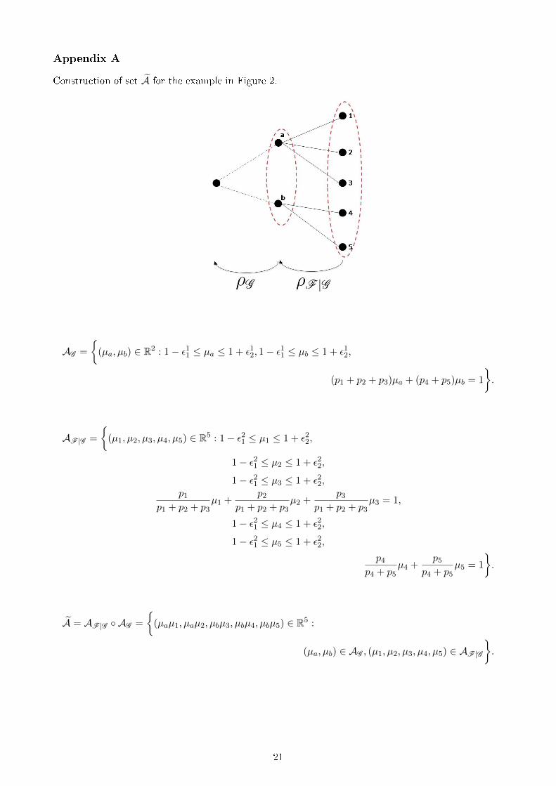
Appendix A
Construction of set A for the example in Figure 2.
AG =
(µa, µb) ∈ R2 : 1− ε11 ≤ µa ≤ 1 + ε12, 1− ε11 ≤ µb ≤ 1 + ε12,
(p1 + p2 + p3)µa + (p4 + p5)µb = 1
.
AF |G =
(µ1, µ2, µ3, µ4, µ5) ∈ R5 : 1− ε21 ≤ µ1 ≤ 1 + ε22,
1− ε21 ≤ µ2 ≤ 1 + ε22,
1− ε21 ≤ µ3 ≤ 1 + ε22,p1
p1 + p2 + p3µ1 +
p2
p1 + p2 + p3µ2 +
p3
p1 + p2 + p3µ3 = 1,
1− ε21 ≤ µ4 ≤ 1 + ε22,
1− ε21 ≤ µ5 ≤ 1 + ε22,
p4
p4 + p5µ4 +
p5
p4 + p5µ5 = 1
.
A = AF |G AG =
(µaµ1, µaµ2, µbµ3, µbµ4, µbµ5) ∈ R5 :
(µa, µb) ∈ AG , (µ1, µ2, µ3, µ4, µ5) ∈ AF |G
.
21
ρG ρF |G
ρG ρF |G ε11 ε12 α1 ε21 ε22 α2
Bound 1 ρ E ε1 ε2 α 0 0 0
Bound 2 ρs ρs 1−√
1− ε1√
1 + ε2 − 1√
1+ε2−1√1+ε2−
√1−ε1
1−√
1− ε1√
1 + ε2 − 1√
1+ε2−1√1+ε2−
√1−ε1
Bound 3 E ρ 0 0 0 ε1 ε2 α
Table 1: Possible choices of ρG (·) and ρF |G (·) that can be used to obtain lower bound on mean-CVaRrisk measure ρ(·).
S S ′
Bound 1 3.5 2.5
Bound 2 3.12 3
Bound 3 3 3.5
Table 2: Values of Bounds 1,2 and 3 for Example 1.
Partition S1 S2 S3 S4
index1 ω1, ω2, ω3, ω4 ω5, ω6, ω7, ω8 ω9, ω10, ω11, ω12 ω13, ω14, ω15, ω16index2 ω1, ω5, ω9, ω13 ω2, ω6, ω10, ω14 ω3, ω7, ω11, ω15 ω4, ω8, ω12, ω16similar ω9, ω4, ω11, ω6 ω7, ω16, ω13, ω1 ω10, ω2, ω8, ω3 ω12, ω14, ω15, ω5dierent ω9, ω7, ω10, ω12 ω4, ω16, ω2, ω14 ω11, ω13, ω8, ω15 ω6, ω1, ω3, ω5
Table 3: Dierent scenario partitions S = S1, S2, S3, S4 for the example scenario tree in Figure 3.
22
J=
2J=
4J=
10
index1
index2
similar
dierent
index1
index2
similar
dierent
index1
index2
similar
dierent
LBchoice
αε 1
Gap
Tim
eGap
Tim
eGap
Tim
eGap
Tim
eGap
Tim
eGap
Tim
eGap
Tim
eGap
Tim
eGap
Tim
eGap
Tim
eGap
Tim
eGap
Tim
e
ρE
0.9
0.8
10.86%
7.1
12.45%
16.5
9.34%
11.1
12.54%
13.4
9.45%
2.0
13.07%
6.9
7.71%
2.1
13.71%
6.4
4.26%
7.8
18.54%
9.7
5.10%
6.6
16.99%
6.0
0.5
7.64%
24.5
8.81%
24.8
7.92%
29.6
8.67%
23.9
6.85%
3.1
9.36%
8.6
7.97%
2.5
9.78%
8.5
3.63%
9.7
11.93%
8.6
7.01%
7.2
12.73%
5.4
0.3
5.32%
18.2
5.79%
52.6
6.56%
95.3
5.69%
48.2
4.91%
4.1
6.33%
13.4
8.29%
3.7
6.73%
11.7
3.01%
11.4
8.34%
7.9
8.32%
7.3
8.28%
7.3
0.8
0.8
9.61%
13.2
10.82%
21.9
7.16%
14.2
10.97%
24.0
8.14%
3.3
11.69%
9.6
5.32%
3.7
11.58%
10.1
3.46%
8.2
15.55%
10.3
6.89%
8.9
14.43%
5.5
0.5
6.57%
22.0
7.20%
55.0
6.28%
116.0
7.40%
31.9
5.81%
4.0
7.80%
11.2
6.05%
3.3
8.15%
11.4
3.00%
9.8
9.89%
8.8
7.83%
7.2
10.51%
5.7
0.3
4.44%
26.6
4.75%
88.6
5.46%
118.9
4.88%
99.2
4.12%
5.0
5.21%
14.9
7.01%
4.8
5.56%
13.8
2.59%
12.2
6.74%
8.0
8.68%
7.5
6.71%
7.5
0.7
0.8
8.86%
21.2
10.11%
74.9
5.35%
24.2
10.10%
44.4
7.60%
4.0
10.49%
12.0
5.33%
4.5
10.51%
12.6
3.85%
7.7
13.09%
9.1
7.82%
7.6
12.70%
7.1
0.5
5.90%
31.5
6.56%
73.7
5.11%
74.2
6.62%
89.7
5.24%
4.3
6.98%
16.3
6.31%
4.2
7.35%
14.9
3.08%
12.1
8.22%
8.5
8.45%
7.3
9.17%
7.5
0.3
3.95%
36.4
4.27%
114.0
4.73%
144.6
4.29%
139.9
3.70%
5.6
4.50%
17.0
7.08%
5.4
4.80%
17.2
2.48%
14.5
5.50%
8.5
8.91%
7.8
5.81%
10.6
ρsρs
0.9
0.8
4.52%
7.2
5.52%
14.8
7.57%
8.3
5.10%
9.6
4.38%
1.6
5.99%
6.1
9.83%
1.8
6.03%
6.3
4.20%
6.7
8.95%
4.4
14.27%
6.8
8.76%
5.2
0.5
3.99%
10.6
4.43%
18.5
7.80%
16.6
4.23%
15.5
3.86%
2.3
4.91%
6.9
10.97%
1.7
5.13%
6.2
4.04%
9.9
7.18%
4.6
13.95%
7.3
7.67%
4.1
0.3
3.08%
20.4
3.14%
21.5
6.57%
66.6
3.02%
20.1
3.04%
4.0
3.56%
7.4
10.47%
3.2
3.79%
10.6
3.38%
10.5
5.31%
6.0
12.83%
7.4
5.18%
4.3
0.8
0.8
3.67%
12.5
4.45%
18.9
6.16%
17.3
4.40%
19.9
3.66%
4.1
5.06%
8.5
10.85%
2.2
5.06%
8.9
3.35%
8.5
7.58%
5.5
14.81%
8.7
7.41%
3.8
0.5
3.30%
12.9
3.52%
22.0
6.68%
34.7
3.40%
59.3
3.12%
3.7
4.01%
10.2
9.91%
2.8
4.09%
9.6
3.09%
9.2
5.94%
5.4
13.86%
7.4
5.98%
4.8
0.3
2.46%
21.1
2.49%
60.9
5.83%
166.9
2.41%
44.2
2.44%
4.2
2.85%
12.3
9.28%
4.1
2.98%
12.8
2.67%
10.3
4.26%
7.0
12.41%
7.6
4.07%
5.6
0.7
0.8
3.37%
21.0
4.40%
19.8
5.10%
22.0
4.22%
28.6
3.39%
4.5
4.68%
11.1
10.73%
4.7
4.90%
8.5
3.80%
7.8
6.18%
5.1
15.10%
7.7
6.53%
3.8
0.5
2.94%
25.1
3.26%
46.0
6.09%
52.5
3.10%
47.1
2.82%
6.1
3.62%
14.7
10.17%
3.4
3.63%
13.7
3.06%
10.2
4.72%
5.0
13.80%
7.3
5.12%
4.9
0.3
2.30%
21.9
2.19%
73.9
5.57%
169.8
2.10%
95.8
2.26%
7.1
2.49%
15.2
9.50%
3.5
2.57%
16.4
2.39%
12.4
3.36%
7.0
12.46%
7.9
3.50%
8.8
Eρ
0.9
0.8
1.15%
6.4
0.65%
5.6
11.78%
6.8
0.36%
5.8
1.97%
2.9
1.10%
3.8
20.35%
1.9
1.00%
3.1
6.81%
9.3
3.80%
4.0
25.67%
6.7
4.31%
3.4
0.5
1.26%
4.8
0.42%
11.9
9.54%
5.6
0.26%
9.1
1.82%
2.4
0.82%
4.3
16.15%
1.6
0.94%
4.4
5.09%
7.4
2.99%
3.1
20.73%
7.3
2.92%
3.1
0.3
1.16%
9.2
0.43%
14.4
7.67%
14.7
0.29%
14.1
1.51%
3.1
0.76%
6.8
13.31%
2.0
0.90%
6.8
3.88%
10.7
2.41%
4.1
17.00%
7.4
2.00%
3.3
0.8
0.8
0.59%
10.0
0.25%
10.2
10.95%
8.9
0.15%
10.9
1.23%
4.5
0.59%
6.9
18.86%
2.8
0.56%
7.4
5.17%
10.9
2.54%
4.1
24.29%
8.8
2.10%
3.9
0.5
0.64%
11.3
0.27%
15.3
8.74%
16.8
0.12%
12.3
1.07%
3.2
0.59%
6.2
14.79%
1.9
0.52%
7.0
3.78%
9.2
2.08%
3.6
19.49%
7.3
1.89%
3.2
0.3
0.60%
16.5
0.27%
17.8
7.13%
58.0
0.19%
18.8
1.04%
3.5
0.53%
7.1
12.36%
2.5
0.47%
8.5
2.94%
10.4
1.69%
4.4
15.95%
7.7
1.36%
4.4
0.7
0.8
0.74%
11.2
0.26%
14.9
10.70%
13.0
0.23%
13.2
1.04%
4.3
0.49%
7.6
17.62%
4.5
0.45%
7.8
4.09%
8.0
1.72%
4.2
22.96%
7.8
1.77%
3.7
0.5
0.63%
16.9
0.26%
14.7
8.47%
22.0
0.22%
18.2
0.87%
3.4
0.51%
7.3
14.15%
3.0
0.47%
8.3
3.02%
9.9
1.35%
3.4
18.68%
7.2
1.52%
3.1
0.3
0.58%
40.8
0.23%
28.2
7.02%
71.0
0.13%
29.0
0.93%
5.8
0.47%
10.1
11.91%
4.3
0.40%
11.6
2.37%
12.6
1.25%
5.4
15.47%
7.9
1.27%
7.7
Table4:
Average
optimalitygapandrunn
ingtimevalues
oftheproposed
algorithm
forvedierentRAMLSP
-3-30instanceswithdierentpartitionand
lower
bound
choices.
23
J=
4J=
8J=
16J=
32
αε 1
Gap
Tim
eGap
Tim
eGap
Tim
eGap
Tim
e
RAMLSP
-3-64
0.9
0.8
1.02%
68.9
2.42%
55.8
5.02%
44.6
8.13%
82.0
0.5
0.92%
132.6
2.07%
66.2
4.27%
60.9
6.99%
86.1
0.3
0.74%
697.4
1.57%
101.4
3.33%
75.6
5.80%
93.1
0.8
0.8
0.71%
27.5
1.67%
13.0
3.82%
26.3
7.10%
85.2
0.5
0.66%
97.4
1.55%
25.4
3.19%
39.3
6.03%
82.4
0.3
0.60%
376.1
1.20%
49.6
2.53%
55.6
4.76%
86.5
0.7
0.8
0.54%
51.8
1.30%
14.5
2.82%
37.6
5.67%
82.9
0.5
0.56%
129.2
1.12%
27.4
2.37%
48.2
4.74%
81.9
0.3
0.48%
373.1
0.93%
63.7
1.96%
57.6
3.73%
84.9
RAMLSP
-4-8
0.9
0.8
5.92%
10.4
6.05%
9.0
9.62%
17.6
11.23%
37.5
0.5
5.49%
16.9
6.69%
19.3
7.28%
26.0
9.18%
59.1
0.3
4.06%
21.3
5.87%
27.0
6.45%
37.8
7.76%
66.5
0.8
0.8
3.59%
13.9
5.03%
11.2
6.69%
18.8
9.62%
50.0
0.5
3.64%
18.6
5.53%
25.5
6.35%
33.2
8.26%
63.5
0.3
3.40%
22.3
5.28%
29.3
5.86%
40.9
7.48%
62.0
0.7
0.8
3.48%
16.0
4.95%
14.5
6.14%
22.0
8.38%
54.3
0.5
3.19%
21.1
5.31%
24.4
5.92%
33.7
7.95%
61.8
0.3
3.12%
28.3
4.86%
32.2
5.54%
41.1
7.09%
65.1
RAMLSP
-5-4
0.9
0.8
6.55%
8.9
10.25%
4.8
13.24%
11.7
16.09%
29.9
0.5
5.53%
13.7
9.09%
5.6
11.69%
16.0
13.27%
43.2
0.3
5.12%
17.1
7.97%
8.0
10.02%
20.0
11.38%
48.2
0.8
0.8
6.83%
9.9
10.78%
4.7
13.40%
11.3
16.16%
29.6
0.5
5.70%
13.6
9.48%
6.2
11.81%
14.9
13.40%
43.7
0.3
5.28%
16.4
8.27%
8.6
10.08%
17.4
11.53%
50.1
0.7
0.8
6.04%
10.3
9.92%
6.0
13.04%
17.0
14.58%
40.5
0.5
5.39%
11.7
8.96%
6.7
10.96%
20.9
12.49%
51.4
0.3
4.93%
15.5
7.94%
9.8
9.53%
22.5
11.00%
56.9
Table
5:Average
optimalitygapandrunn
ingtimevalues
oftheproposed
algorithm
forvedierentRAMLSP
-3-30,
RAMLSP
-4-8
andRAMLSP
-5-4
instanceswithpartitiondierentandlower
bound
choice
Eρ.
24
Proposed Algorithm DEP with CPLEX
α ε1 Gap Time Gap_CPLEX Looseness Time_CPLEX Delay
0.90.8 1.02% 68.9 2.76% 2.71 248.3 3.60
0.5 0.92% 132.6 3.47% 3.78 2366.7 17.84
0.3 0.74% 697.4 1.39% 1.89 719.9 1.03
0.8
0.8 0.71% 27.5 2.04% 2.87 241.9 8.79
0.5 0.66% 97.4 1.48% 2.24 403.9 4.15
0.3 0.60% 376.1 0.89% 1.47 603.0 1.60
0.7
0.8 0.54% 51.8 2.47% 4.58 246.4 4.75
0.5 0.56% 129.2 1.13% 2.01 444.2 3.44
0.3 0.48% 373.1 0.81% 1.70 1445.6 3.87
Table 6: Comparison of optimality gap and running time of the proposed algorithm and CPLEX.
25
Recommended