A STUDY OF RUTTING OF ALABAMA ASPHALT PAVEMENTS
Final Report Project Number ST 2019-9
by
Frazier Parker, Jr. E. Ray Brown
Auburn University Highway Research Center Auburn University, Alabama
sponsored by
The State of Alabama Highway Department Montgomery, Alabama
August 1990
The contents of this report reflect the views of the 'authors who are
responsible for the facts and accuracy of the data presented herein. The
contents do not necessarily reflect the official views or policies of the State of
Alabama Highway Department or Auburn University. This report does not
constitute a standard, specification, or regulation.
2
ABSTRACT
Pavement rutting is the accumulation of permanent deformation in all or a
portion of the layers in a pavement structure that results in a distorted
pavement surface. The overall objec~ive of this study was to develop
recommendations for more rut resistant asphalt concrete mixtures which
comprise the uppermost layers of flexible pavements. To accomplish project
objectives a plan of study was conducted that included 1) an analysis of rutting
data from the Alabama Highway Departments pavement condition data base, 2) a
field evaluation and sampling program at thirteen test sites, 3) a laboratory
testing program, and 4) analyses of data from the field and laboratory testing
programs.
The analysis of the pavement condition data base indicated that rutting is
increasing and that rutting susceptibility varies geographically because of the
variable quality of locally available aggregate. Careful control of crushing of
gravel and the development of a test to quantify and limit particle shape and
texture of fine aggregate were identified as means for improving aggregate
quality.
In most cases permanent deformation appeared to be combined to the top
three or four inches of asphalt aggregate layers, thereby, implicating high tire
pressures as the primary causative factor. A rate of rutting of 2 x 10⁻⁴
in/--iESAL or 1.0 x 1 0-7in/ESAL delineated good and poor performing pavements.
Mix and aggregate properties that appeared to be related to rutting ir'clude:
layer thickness, voids, GSI, gyratory roller pressure, percent fractured faces,
percent passing No. 200 sieve and creep strain. The correlation of these
properties was not very strong, but in almost every case was caused by one or
two points far outside the range of the bulk of the data. This illustrates the
complexity of the rutting process and the necessity of considering a number of
properties during material selection and mix design.
3
TABLE OF CONTENTS
Introduction .............. ............... ............................................... ................................. ........ 5
Objectives ......................... ............................................................................................... 8
Scope ............................................................................................................................... 9
Plan of Study ................................................................................................................... 1
Presentation and Analysis of Results ......................................................................... 19
Conclusions and Recommendations.. ............ ...... .................. ............ ................ ....... 45
References ...................................................................................................................... . 47
Tables .............................................................................................................................. 49
Figures ............................................................................................................................. 62
Appendix A, Rutting Data from Pavement Condition Databases ......................... 104
Data Sorted by AHD Division ........................................................................... 105
Data Sorted by Mix Type ................................................................................... 115
Frequency Distributions ..................................................................................... 125
Appendix B, Layer Profiles from Field Test Sites .................................................... 132
4
INTRODUCTION
Pavement rutting is the accumulation of permanent deformation in all or a
portion of the layers in a pavement structure that results in a distorted
pavement surface. Longitudinal variability in the magnitude of rutting causes
roughness. Water may become trapped in ruts resulting in reduced skid
resistance, increased potential for hydroplaning and spray that reduces
visibility. Progression of rutting can lead to cracking and eventually complete
disintegration.
Flexible pavement rutting is not a new problem. As long as flexible
pavements have been used, rutting has been recognized as a primary distress
mechanism and a primary design consideration. For high flotation tires rutting
may be confined to weaker materials such as subbases and subgrade soils. In the
not to distant past, the consensus was that rutting was generally restricted to
subgrades. In fact, the 1986 AASHTO Guide for Design of Pavement structures is
based on performance models developed at the AASHO Road Test where tire
inflation pressures were nominally 80 psi. Asphalt pavement design concepts
are based on providing sufficient pavement structure (rutting resistant
materials) to reduce stresses in the subgrade to the pOint where rutting will not
develop, and on providing asphalt quality and thickness to resist fatigue
cracking.
What is new regarding flexible pavement rutting is the awareness that
permanent deformation in the high quality asphalt layers (surface, binder and
base) has become a significant contributor to pavement rutting. No where is this
more vividly demonstrated than in rutting of asphalt concrete overlays of
Portland cement concrete pavements.
Repetitive applications of heavy trucks with increasingly high pressure
tires drives rut formation in high quality asphalt layers. The stresses induced in
5
near surface layers by the high pressure tires exceed the ability of the materials
to resist densification below critical voids (4%) and subsequent plastic flow.
Recent studies (1-5) have shown that truck tire inflation pressures, and
therefore contact pressures, have increased dramatically from 80 psi on which
design procedures are commonly based. Average truck tire inflation pressures
for radial tires are now around 100 psi. This means that a significant portion of
truck tires have inflation pressures higher than 100 psi, often in the 130 to 140
psi range.
The study by Marshek, Chen, Connell and Hudson (6) notes several additional
problems with high tire pressures. A commonly made assumption has been that
contact pressure approximately equals inflation pressure. The study showed that
increased tire pressure produced proportionally smaller gross contact areas.
This suggests that the commonly made assumption of equal pressure becomes
increasingly less valid. The study also showed that contact pressures were not
uniform. This suggests some contact areas with pressures greater than a
uniform pressure based on gross contact area.
Extraordinarily high tire pressures mean that asphalt concrete layers which
are of the highest quality but nearest to the surface in a pavement structure are
not immune to rutting. Although recent modifications such as asphalt content
selection based on 75 blow Marshall compaction have increased rutting .
resistance, material quality provided by existing specification occasionally is
insufficient to meet the demands of today's traffic.
Assuming that truck volume, loading and tire pressures are not likely to
decrease; the obvious solution is to increase asphalt concrete resistance to
permanent deformation. As with most simple and obvious solutions it must,
however, be approached with caution. Beneficial changes in one property may
lead to detrimental changes in another property. For example, decreasing asphalt
6
content will result in increased rutting resistance, but decreased fatigue
resistance. Increased asphalt cement viscosity will result in a stiffer mix,
which may be more resistant to rutting, but a mix that is more likely to crack
(traffic and environmental forces).
In Alabama the solution is complicated by available materials. Local
natural sand and gravel are used extensively, particularly in the southern and
western portion of the state. These materials generally have rounded particle
shape which is detrimental to mix stability. Even when gravel is crushed, the
larger particles that result are likely to have at least one uncrushed face since
the maximum particle size of available natural gravel is around 1-1/2 inches.
The solution to the rutting problem in Alabama will likely not be obvious or
simple but will require careful consideration and treatment of the entire
problem. However, a solution, or even small improvemnts, are potentially
enormously Significant; considering the dominant role asphalt concrete will play
in rehabilitating and upgrading the states over 10,000 miles of roadway. Of
particular significance will be the requirements of the approximately 900 miles
of interstate pavement which carries a disporportionately large volume of truck
traffic.
7
OBJECTIVES
The overall objective of this study was to develop recommendations for
more rut resistant asphalt concrete mixtures. To accomplish this overall
objective the following five sub-objectives were:
To determine the nature and extent of rutting on Alabama Highways,
To conduct testing and evaluation of typical asphalt concrete mixtures,
To characterize mixtures that are susceptible to rutting and those that are not susceptible to rutting,
To review Alabama Highway Department (AHD) material selection and asphalt concrete mix design procedures, and
To formulate recommended modifications to current practices to enhance resistance of asphalt concrete mixes to permanent deformation.
8
SCOPE
The assessment of the nature and extent of rutting of asphalt pavements in
Alabama was limited to an analysis of data from the 1984, 86, and 88 Alabama
Highway Department pavement condition data bases. These data bases are part
of the overall pavement management system being implemented by the Alabama
Highway Department.
Testing and sampling was conducted at thirteen (13) test sites. Sites were
selected to provide materials with a range of rutting resistance. Test pits were
dug through and cores taken of all asphalt-bound layers. Laboratory testing of
materials from the cores measured properties to characterize in-situ mix,
recompacted mix, recovered aggregate and recovered asphalt cement.
Efforts to improve rutting performance of Alabama asphalt pavements were
focused on consistant material selection and mix design for asphalt concrete.
Consideration of structural pavement thickness design and construction aspects
were beyond the scope of the study.
9
PLAN OF STUDY
To accomplish project objectives a three (3) phase study was executed. The
three phases consisted of 1) an analysis of rutting data from the Alabama
Highway Department's pavement condition data base, 2) field evaluation and
sampling at thirteen test sites, and 3) a program of laboratory testing. Data
from these studies was analyzed to develop a model for describing the rutting
process and to formulate recommendations for improving the rutting resistance
of asphalt concrete mixes.
Rutting Data from Pavement Condition Database
Condition and traffic data for the Alabama state and interstate system are
collected from representative 200' long test sections in each lane mile of
pavement. Data collection procedures are described in reference 7. Data
collection was initiated by the Department in 1984 and has been repeated in
1986 and 1988. Data records for each lane mile contain identifying and
descriptive information, quantitative pavement condition information (including
rutting), pavement ratings developed from condition data, present serviceability
indices (PSI) developed from roughness measurement, and estimated traffic data.
Eight rut depth measurements, four in the outer wheel path and four i'n the
inner wheel path, are taken in 200' test sections for each lane mile of pavement.
A four foot long straight edge is placed across the wheel path and the maximum
rut depth measured. For this study these eight measurements were averaged and
used to represent the rutting for each lane mile of pavement. Reference is made
in the remainder of the text to average rut depth. Measurements were made in
all lanes, but rut depths in outer lanes were always larger and were used
exclusively in the analyses.
In the analyses, estimates of the traffic applied to the pavement were in
-- terms of total numbers of 18 kip equivalent single axle loads (ESAL). Eighteen
10
kip ESAL's were computed for two and four lane roadways using equations 1 and
2, respectively.
where
ESAL = (AADT)(CV)(0.5)(Age)(0.82)
ESAL = (AADT)(CV)(0.5)(Age)(0.82)(0.85)
AADT = Annual average daily traffic
CV = Percent commercial vehicles as decimel
= Directional split
.. ................. (1)
................... (2)
0.5
Age = [(year + month rated) - (year + month bUilt)]365 12 12
0.82
0.85
= Average conversion factor from reference 8
= Percent traffic in outer lane for 4-lane roadway
The annual average daily traffic and percent commercial vehicles used in
the computation of ESAL's were the estimated values for the year in question.
Traffic was assumed split evenly by direction (SO/50). The pavement age, in
days,. was the difference between the date rated and the date the last surface
layer was placed. For older pavements and pavements with significant traffic
growth, this procedure will have over estimated total applied traffic. However,
since most of the comparisons were relative this is not considered a serious
problem that would warrant a more accurate estimation of traffic.
To determine the nature and extent of rutting three parameters were
analyzed. These were average rut depth, mean (average rut depth/ESAL) and
mean average rut depth/mean ESAL. The ratios of average rut depth to ESAL and
mean average rut depth to mean ESAL provide indicators of the rate of rut
formation with traffic. Comparisons of the three variables were made between
Highway Department Divisions to detrmine if geographical differences exist, and
between surface mix types. Data for these comparisons were grouped according
1 1
to roadway type (state routes, interstate routes and combined) for the 1984, 86
and 88 data bases. The data was also combined for overall comparisons.
Frequency analyses of average rut depth and (average rut depth)/(ESAL) were
made to determine if the distribution of rutting is changing and if rutting
severity is a function of roadway type (state or interstate routes).
Field Evaluation and Sampling
Thirteen test sites were selected for evaluation and testing. The
approximate location of these sites is shown on Figure 1. Sites were selected to
provide a relatively uniform statewide geographic distribution. Sites were also
selected to provide examples in the Piedmont and Applachian Plateau geologic
regions where crushed stone is available, and in the Coastal Plain geologic region
where natural sands and gravels are the predominate aggregate used in hot mix·
asphalt. The sites were selected to provide a range of rutting performance. Five
(5) sites were considered by Highway Department personnel to have provided
good rutting performance and eight (8) to have provided poor rutting
performance.
The development of rutting was investigated by cutting a trench and coring
through all asphalt bound layers. All test sites were on four lane facilities and
the trenches and cores were taken across outside lanes only. A typical sampling
layout is shown in Figure 2. Two lines of 12 cores each, one of 4-inch cores and
one of 4 and 6-inch cores, were cut.
Pavement surface profiles at the trench and at core lines were obtained by
measuring the distance from a leveled 12 foot long straightedge as illustrated in
Figure 3a. Once the trench was cut, similar measurements were made to layer
interfaces, as illustrated in Figures 3b and 3c, to obtain a complete profile for
all the asphalt-bound layers. Layer thicknesses were measured from cores
(Figure 3d) and added to surface profile measurements as a second method for
12
developing complete layer profiles. Cores were then used to provide material for
the laboratory testing program described in the following section.
Laboratory Testing
There are a number of laboratory tests that have been used to predict
rutting in asphalt pavements. These tests cannot be used individually in all
cases to identify mixtures with a tendancy to rut under traffic, but all the tests
combined have been shown to be a fairly good indicator of rutting. Tests that
will be used in this study to correlate with rutting include: voids in place, voids
in laboratory compacted samples, stability and flow of laboratory compacted
samples, aggregate gradation, fractured face count of coarse aggregates,
particle shape and texture of fine aggregate, gyratory shear index (GSI), gyratory
roller pressure, creep, resilient modulus, and asphalt cement properties.
In Place Properties. Past studies have shown that in-place air voids are
related to rutting (9,10,11). Most data indicates that once the air voids decrease
to 3 percent or lower plastic flow is likely to occur. The in-place voids alone
may not be a good predictor of rutting since some mixes with low voids do not
rut and some mixes with higher voids do rut.
It has also been shown that in-place voids may decrease to a point and then
increase again as rutting progresses. This increase of in-place voids during
traffic makes it difficult to correlate rutting with in-place voids. For instance
rutting may have been caused by low in-place voids but measurement of in-place
voids may show higher voids if the voids increase when rutting begins. This
process will be considered later during development of the model to describe
rutting.
Approximately 24 cores were taken at each test, as illustrated in Figure 2.
A number of the cores were combined and broken-up for tests such as Rice
specific gravity, gradation, asphalt content, and recompacting. The bulk density
13
of cores were then compared to the measured Rice specific gravity to determine
in-place voids.
Properties of Laboratory Compacted Samples. Samples of asphalt
mixture were combined, broken-up, heated and recompacted to evaluate
properties of laboratory compacted samples. The properties of laboratory
compacted samples is an indicator of original mix design properties. The
Marshall stability will always be higher than the original mix design because the
asphalt cement is now stiffer due to oxidation, however, the voids and flow
appear to be approximately equal to those measured during mix design.
The use of voids of recompacted mix does have some advantage over use of
in-place voids. For instance the in-place voids will vary across the traffic lane
due to traffic and the in-place voids may actually begin to increase as rutting
occurs. In-place voids are also a function of original density and traffic. Thus,
in-place voids are dynamic (changing) and will vary depending or many factors
making it difficult to predict performance. Recompacted voids on the other hand
are more consistent and should be representative of the final in-place voids
after Significant traffic. Hence, recompacted voids may be a better indicator of
rutting potential than the in-place voids. Samples were· recompacted in two
ways: hand hammer and gyratory.
Seventy-five blows per side with the hand hammer has been shown to
provide a density approximately equal to that after traffic for high volme roads.
Work with the gyratory testing machine (GTM) has shown that it provides a
density approximately equal to that of the hand hammer when it is set at 120 psi
(approximately equal to truck tire pressure), 1 degree angle, and gyrated for 300
revolutions.
Two additional properties of the asphalt mixture that are evaluated when
using the GTM to recompact samples include gyratory shear index (GSI) and roller
14
pressure (a measure of shear strength). Past studies have shown the GSI to be
related to rutting. Mixes with a GSI equal to approximately one tend to be
resistant to rutting while mixes with a GSI above about 1.3 tend to rut severely
under traffic. Since the roller pressure is a rough measure of shear strength it
potentially could relate to rutting.
Extracted Aggregate Properties. Mix from cores was separated into
aggregate and asphalt cement components. Gradation, fractured face counts on
coarse aggregate particles, and fine aggregate particle shape and texture tests
were conducted on extracted aggregate.
The aggregate gradation of a mixture is important but there is disagreement
about the gradation that should be used. Most people agree that the aggregate
gradation should be approximately parallel to the maximum density curve, but
should be offset to provide sufficient VMA. Some agencies specify that the
gradation be above the maximum density curve while others specify that it be
below the curve.
It is difficult to quantify and evaluate an aggregate gradation since 8-10
sieve sizes are normally used. In this study three sieve sizes will be used to
evaluate gradation: 3/8 inch, No. 50, and No. 200. These three sieve sizes should
be sufficient to accurately charaterize the aggregates gradation.
Studies have shown that the maximum aggregate size is important for rut
resistant pavements. Larger maximum aggregate size mixtures are more
resistant to rutting while finer mixtures tend to rut more. Mixtures with
excessively high or low amounts of material passing the No. 200 sieve are more
likely to rut. Mixtures with high natural sand content are also more likely to rut.
The three selected sieve sizes should be sufficient to evaluate maximum
aggregate size, percent passing No. 200, and amount of natural sand.
15
It has long been known that crushed aggregates produce mixes that are more
resistant to rutting than mixes with natural aggregate that has more rounded
particles. It is not clear however what the optimum fractured face count should
be to insure good performance. AHD 1989 specifications have crushed particle
requirements on minus 3/4" to plus No.8 material when gravel is used in binder
mixes and a requirement that 80% of the plus No.4 particles used in wearing
courses have two or more crushed faces. The problem with rounded aggregate
can occur when gravels or natural sands are used since both of these may be the
desired size without crushing.
The fractured face count was conducted on the plus No.8 material. The
percent of aggregate particles with zero, one, or two or more crushed faces were
recorded. The material smaller than the No.8 could not be tested since it was
too small to evaluate the number of fractured faces.
Resilient modulus has become popular in recent years to characterize the
stiffness properties of asphalt concrete. The test to measure resilient modulus
is repeated load indirect tensile. Since resilient modulus is a tensile test it
should be affected by changes in asphalt cement properties, but it is doubtful if
it can be correlated to rutting since this is the result of shear strain in an
asphalt mixture.
Tests were conducted on cores cut from the pavement. The test was
performed by applying approximately 15% of the tensile strength for 0.1 seconds
and allowing the asphalt mixture to recover for 0.9 seconds. Tests were
conducted at 40,77, and 104°F to establish temperature sensitivity.
It is generally believe that the creep test has potential to model rutting of
asphalt mixes. The creep test is typically conducted at various temperatures.
Compression loads can be applied statically or repetitively to unconfined or
confined specimens. The most common mode is the static unconfined mode,
16
because it is the easiest and simplest. However, this mode probably does the
worst job of simulating what actually happens in the field.
Two major problem with the static unconfined test is that the temperature
cannot be as high as 140°F (typical in-place temperatures) and the normal
pressure must be much lower than 120 psi (typical truck tire pressures). High
temperature or high pressures in unconfined tests will result in
unrepresentative failure of the sample. For this study all tests were conducted
in the static confined mode. Tests were conducted at a pressure of 120 psi and a
temperature of 140°F. A confining pressure of 20 psi was used. When a
particular asphalt layer was being investigated that was less than two inches
thick, two or more cores were stacked to insure that a total thickness of at
least two inches was obtained. When cores were stacked, cement mortar was
applied between the cores to provide proper seating.
The shape and texture of fine aggregate particles is thought to be as
important as the shape of coarse aggregate particles. A test for particle shape
and texture of minus No.8 material proposed by the National Aggregates
Association (12) was conducted. Uncompacted voids of a graded samples (Method
A) were measured.
In addition, 400 gm samples of ungraded minus No.8 material were run
through the apparatus and flow times recorded. These modified tests were
performed because the uncompacted voids from Method A did not provide a wide
range of values. It was felt that flow time might provide a wider range of values
and better correlation with rutting susceptibility, but it did not.
Extracted Asphalt Cement Properties. The aggregate must support the
load if rutting is prevented in asphalt concrete, however, the asphalt cement
properties can also affect performance. If the asphalt mixture has a slightly
high asphalt content, then the asphalt cement properties can greatly affect rate
17
of rutting.
Asphalt cement was recovered from cores and tested for viscosity and
penetration. Viscosity testing was conducted at 140° and 275°F, and penetration
testi ng at 77 and 40° F.
18
PRESENTATION AND ANALYSIS OF RESULTS
Data and analyses of these data from the three phases of the study
described in the preceding section are presented individually in this section.
These analyses are then combined and a model proposed for describing rutting of
asphalt-bound layers of flexible highway pavements.
Analysis of Rutting Data from Pavement Condition Database.
The rutting data in the 1984, 1986, and 1988 pavement condition data bases
were analyzed to assess the nature and extent of the rutting problem in Alabama.
As noted earlier, the data will be grouped and compared to isolate the effects of
various parameters.
Combined Data. Table 1 contains a summary of all data from the 1984,
1986, and 1988 databases. The data is grouped according to roadway type (state
routes, interstate routes and combined). Column 2 contains the frequency which
is indicative of the number of lane miles of pavement. Column 3 contains the
mean of average rut depths, Column 4 the ratio of the m,ean average rut depth to
mean EASL, and colum 5 the mean of the average rut depth to ESAL ratio.
Values from Table 1 are plotted in Figure 4. From this figure the following
observations can be made:
• Mean rut depths are larger on interstate routes than on state routes.
This is likely due to the larger traffic volumes on interstate routes.
• The average rut depth has increased from 1984 to 1988.
• The average rut depth increase, from 1984 to 1988, is larger for
interstate routes (0.01494 in.) than state routes (0.0036 in.).
• Because of the large frequency for state routes, the average rut depth
for state route and combined data is similar.
• Because of the small frequency for interstate routes, the average rut
depth relationship is more erratic, i.e., the level of the overaly program
19
can have an observable influence on mean rut depth.
• Values of the ratios of the means (b) are considerably different than
values of means of the ratios (c). This is due to the large numeric
differences between numerators (average rut depth) and denominators
(ESAL) and the wide range of ESAL values. Values shown for both
parameters are ratios multiplied by 107.
• Because of the large influence of extreme values of ESAL's, the ratio of
the means is considered a better indicator of rate of rut development.
• Both ratios indicate that the rate of rut development is increasing.
• Both ratios indicate that the rate of rut development is much greater
on state routes than interstate routes. This is likely due to higher
quality pavements (including quality of asphalt bound materials) on the
interstate system.
• The ratios of the means (b) show about the same increase in rate of rut
development, from 1984 to 1988, for state routes (0.188) and for
interstate routes (0.166).
• The mean of the ratios (c) show a much larger increase in rate of rut
development, from 1984 to 1988, for state routes (1 .859) than for
interstate routes (-0.052).
To summarize, all but one of the parameters examined indicated that
rutting is increasing. For rut depth this could be caused by an increase in
pavement rutting susceptibility, an increase in traffic volume or an increase in
loading severity (truck weight and/or tire pressure). For rate of rut
development, possible causes would be restricted to rutting susceptibility and
loading severity.
Highway Department Division. Comparisons by Highway Department
Divisions were made for mean rut depth, the ratio of mean rut depth to ESAL's
20
and the mean of the ratio of average rut depth to ESAL's. These comparisons
were made to determine if geographical variations in rutting exists and to
examine possible reasons for these variations. Speculation was that geology
and, thus, the availability of variable quality aggregates might be a factor. As
shown in Figure 1, Divisions 1, 3 and 4 are predominately in the Piedmont and
Appalachian Plateau geologic provinces. Rock deposits in these areas are used
for crushed stone and are the source of sand and gravel materials. Division 2 is
divided between the Appalachian Plateau and the Coastal Plain region.
Divisions 5-9 lie below the Fall Line in the Coastal Plain region. Natural
sands and gravels are available and are the predominate aggregate materials
used in this region. The degree of weathering and, thus, particle size and shape
of sand and gravel is influenced by the distance transported from the source
material. Particles become more rounded and smaller as the transportated
distances increases. Implications are that aggregate quality and, therefore, mix
rutting susceptibility increases with movement southward as the distance from
the rock source increases.
For natural sand (fine aggregate) and uncrushed gravel (coarse aggregate)
in asphalt bound materials, the influence of particle size and shape is straight
forward and well established. However, when gravel is crushed, the influence of
gravel size is not as direct or as well documented. Coarse aggregate for surface
and binder mixes is required to have some crushed particles. Therefore, natural
gravel requires crushing. The problem created by using gravels is that the degree
of particle fracturing will be directly related to original particle size. Smaller
gravel particles will be less fractured and mixes containing these partially
crushed particles will be more susceptible to rutting.
If indeed geology and, thus, geography is a factor, rutting susceptibility
should be less in Divisions 1-4 than in Divisions 7-9. Divisions 5 and 6 should be
21
intermediate. Figure 5 shows three histograms which illustrate the variability
of rutting susceptibility between divisions. From the three histograms, it can be
seen that the rut depth, ratio of mean rut depth to mean ESAL's and mean of the
ratio of average rut depth to ESAL's are less for Divisions 1-4 than for Divisions
5-9. The averages of the three parameters for Divisions 1-4 are 0.07380 in,
1.286 inches x 10-7 and 8.510 inches x 10-7. For divisions 5-9 the averages are
0.12759 inches, 2.750 inches x 10-7 and 13.656 inches x 10-7.
The data shown in Figure 5 is from the 1984 database for combined state
and interstate routes. Similar histograms were plotted for 1986 and 1988
databases for state, interstate and combined routes. A complete set of these
histograms is contained in Appendix A. Averages from these histograms are
shown in Table 2, and confirm the trends illustrated in Figure 6 for the 1984
combined data, Le., that pavements in Divsions 5-9 are more susceptible- to
rutting thqn those in Divisions 1-4.
The most consistant indicator of this trend is the ratio of means which is
an indicator of rate of rut development. Rut depth and the mean of the ratio of
rut depth to ESAL's is more sensitive to pavement age. Between 1986 and 1988
the relationship between average rut depth and the mean of the ratio for
combined and state route data reversed.
As can be seen in Table 2, the average 1988 rut depths on state and
combined routes for Divisions 1-4 are about equal those in Divisions 5-9. The
means of the ratios for 1988 become larger in Divisions 1-4. This reversal in
trend is thought to be primarily due to a reversal in values for Divisions 4 and 5.
Figure 6 is similar to Figure 5, but for 1988 data. Comparing Figures 5 and 6, it
can be seen that the mean rut depths and ratios become'larger for Division 4 in
1988; which is opposite what was observed in 1984 and 1986. The number of
ESAL's applied to the pavement is an indicator of pavement age and, therefore, of
22
the overlay program. In 1986 the average number of ESAL's on combined state
and interstate routes in Division 4 was 306,000 and in 1988, 365,000. The trend
in Division 5 was just the opposite, with applied ESAL's going from 450,000 in
1986 to 384,000 in 1988. This reversal in applied traffic (average pavement
age) for Divisions 4 and 5 is thought to be primarily responsible for the reversal
in trends.
Despite the exceptions noted above, the analyses of the data support the
contention that rutting susceptibility is related to geographic location. In
addition, geology and, thus, properties of available aggregate provide a logical
explanation for the observed relationship between rutting susceptibility and
geographic location. This phenomenon will be examined further in the analyses
of the data from field test sites.
Mix Type. Data was grouped by existing surface mix type. Similar mix
types were combined to obtain five mix type groups identified as 401 (surface
treatment), 411,416,417 (latex) and 420 (open graded). Analyses were
performed for the three parameters used previously, Le., average rut depth, mean
rut depth/mean ESAL and mean (average rut depth/ESAL). A complete set of
histrgrams developed to study the influence of mix type on rutting susceptibility
is contained in Appendix A.
Interstate routes are surfaced with primarily 416 mix with some open
graded porous friction course (420) mix. A minimal amount of 417 mix shows up
in 1988 but no 401 or 411 mix is used. Figure 7 shows 1988 interstate data,
which is typical for 1984 and 1986. Average rut depths are about the same for
pavments with 416 and 420 surface mixes. The relationship between the rate of
rutting, as indicated by the ratio of means, for the mixes varies from year to
year. However, the variation is small (minimum of 0.434 x 10⁻⁷ inches to
maximum of 0.672 x 10⁻⁷ inches) indicating that the rate of rutting is similar
23
for both mixes
The mean of the average rut depth to ESAL ratio varies considerably, but
the value for 420 mix is always considerably smaller than 416 mix as shown in
Figure 7. The large difference in age of surfaces with the two mixes is thought
to cause this difference. No 420 mix has been placed recently, and badly rutted
sections are overlaid. This results in a decline in the amount of 420 mix with
only those pavements performing well increasing in age. Pavements are overlaid
with 416 mix, thereby, decreasing or maintaining its age. Since the mean of the
ratios is sensitive to extreme values of rut depth or ESAL's (indicative of age),
the large differences in values is reasonable, but probably not a valid indicator
of the mixes relative rutting susceptibility.
Analyses of all mixes is best accomplished by comparing data for state
routes, considering that state routes are surfaced with all type mixes. Figure 8
shows how usage and rate of rutting for the various mixes is changing with time.
Figure 89 shows that the usage of 401 , 411 and 420 mix is decreasing, and that
the usage of 416 and 417 mix is increasing. For 401, 411 and 416 mix, this
reflects the upgrading of state routes to satisfy increased traffic demands. Use
of 417 mix remains small, but its increased usage is, at least partially,
motivated by the belief that latex improves rut resistance.
The rate of rutting is increasing for 401 and 416 mixes, but appears to be
stabilizing for 411 mix. Traffic loading severity is an obvious reason for this
increase, but as discussed for interstate routes, changes in usage patterns will
influence relative age which may in turn affect the validity of rate of rutting
indicators.
The limited use and age of 417 mix prevents drawing strong conclusions
regarding its performance relative to 416 mix. However, several interesting
trends are apparent from Figure 8. Its use is increasing rapidly, and its rate of
24
rutting is approximately twice that of 416 mix. The relationship between the
rate of rutting of the mixes may be a result of the limited use of 417 mix. As its
use and age increases, its rate of rutting should become more comparable with
416 mix.
Figure 9 shows 1986 data grouped by mix for all three parameters. The
histograms for mean rut depth and mean rut depth/mean ESAL are typical of
1984 and 1988. The data for the mean of the ratio of average rut depth to ESAL
is more erratic, particularly for the 1988 data. Again, this is thought to be
caused by extreme values and adversly affects the parameter as an indicator of
rutting susceptibility. The ratio of means is a more valid indicator of rate of
rutting.
Figure 9 shows that mean rut depths for 401 ,411 and 416 mixes are about
the same. This indicates consistency in the design of materials for the traffic
loading intensities that these mixes are expected to withstand. Rate of rutting,
as measured by the ratio of means, indicates that the rate of rutting for 411 and
416 mixes are about the same. Again this indicates consistency in material
design for expected traffic. Rate of rutting for surface treatments (401) is
higher. This is expected since rutting will develop in base, subbase, and possibly
the subgrade in these pavements. Heavy truck loads and high tire pressures will
be critical for pavements with surface treatments since they provide only .
minimal cover for base and subbase layers. Bases and subbases for these type
pavements are usually comprised of unbound soil aggregate type materials which
will not be particularly rutting resistant.
Rutting Frequency Distributions. Frequency distributions of average
rut depth and rate of rutting, as measured by the ratio of average rut depth to 18
kip ESAL, were analyzed for trends with time and pavement type. A complete set
of frequency distriputions are contained in Appendix A.
25
Figures 10 and 11 show, respectively, 1988 state and interstate rut depth
frequency distributions and 1988 state and interstate rate of rutting frequency
distributions. The shapes illustrated are typical for 1984 and 1986 data. The
rut depth distributions, Figure 10, show, as did Figure 4a, that rut depths are
larger on interstate pavements. The rate of rutting distributions, Figure 11,
show, as did Figure 4b, that the rate of rutting is smaller on interstate
pavements. Figure 11 also shows a much wider range of rate of rutting on state
route pavements. This is expected because of the greater diversity of materials,
pavement structures and traffic on state routes.
Figures 12 and 13 show, respectively, rut depth and rate of rutting
frequency distributions for 1984, 86, and 88 state route data. The trends
illustrated for state routes were generally applicable for interstate routes.
Figure 12 shows a change in shape for the rut depth distribution between 1984
and 1986. This appears to be an indication that the magnitude of rutting was
significantly increasing, but comparison of the cumulative frequencies and
percentages for 1984 and 86 reveal only minor changes. The shape of the 1988
distribution reverts back to the 1984 shape. Figure 13 shows consistent shapes
and only minor changes in frequency for rate of rutting. Although significant
changes with time in rut depth and rate of rutting are not visually apparent from
the frequency distributions, mean values did increase with time as demonstrated
in Figures 4a and c.
Analysis of Field Data.
Data from the thirteen (13) field sites was analyzed to determine where in
the pavement structure permanent deformation was developing and the
relationship between rut development and traffic. The locations of the 13 test
sites are shown in Figure 1 and descriptions of the pavement structures given in
Table 3.
26
Layer Profile Analysis. The profiles of the asphalt bound layers were
analyzed to determine where rutting was developing. When trenches were
opened, string lines were stretched along layer interfaces, as illustrated in
Figure 13, to defect depressions in the lower layer surface. These depressions
would be indicative of permanent deformation in the layer itself or lower layers.
As can be seen from the pavement structure descriptions in Table 3, nine of the
13 pavements were comprised of an original structure plus at least one overlay.
This made the determination of the lower limit of rutting more difficult, but
measurements in the trenches indicated that permanent deformation was
primarily confined to near surface (approximately 4 inch depth) asphalt bound
layers. In most pavements this limited permanent deformation to surface and
binder layers. The interface between binder and black base layers were usually
relatively depression free.
At only Site 9 was there evidence of rutting in base or subbase layers
below asphalt bound layers. There was evidence of rutting in or below the
sand-clay-shell base at this site. When this rutting occurred could not be
determined. It may have developed in the original pavement when cover was only
the "AKG" treatment and approximately one inch of asphalt concrete. Or, it may
have developed later when the structure was thicker, but loads and tire
pressures greater. At only Site 2 was there evidence that stripping may have
contributed to rutting. At this site several cores in wheel paths disintegrated
and could not be completely recovered. Stripping was confined to the original
binder and base layer.
Profiles were also analyzed to determine the magnitude of rutting and
where in the pavement structure permanent deformation was occurring. This
analysis is illustrated in Figure 14. Profiles for all thirteen sites are contained
in Appendix B. Total rutting was determined by averaging rut depths (Ri and Ro)
27
in inner and outer wheel paths at the trench and two core line locations. Rut
depths are compiled in Table 4. Also shown in Table 4 are rut depths for the test
sites compiled from the 1988 pavement condition database. Database rut depths
are smaller primarily because of different measuring methods. A 4-foot
straightedge was used for data base measurements and a 12-foot straightedge
was used at test sites. Data base rut depths are the average of eight
measurements per lane mile for design projects in which test sites were
located. Design projects were several miles long.
The rut depths from Table 4 are plotted as a histogram in Figure 15. From
this histogram the following can be noted:
• Rut depths at sites selected for good rutting performance are
generally less than rut depths at sites selected for poor
performance.
• Rut depths (12 foot straight edge) are generally less than 0.4
inches for sites with good performance and greater than 0.4
inchs for sites with poor performance.
• Rut depths (4 foot straight edge) are generally less than 0.2
inches for sites with good performance and greater than 0.3
inches for sites with poor performance.
While rut depth is an indicator of pavement performance, it is influenced by
traffic (volume and load) which must be considered when assessing rutting
susceptibility. The effects of traffic will be considered in the following
section.
Permanent deformation in various layers was determined analyzing the
shape of layer interfaces. As indicated by stringlining layer interfaces in
trenches, the permanent deformation occurred primarily in upper layers. As
illustrated in Figure 14, strait edges along binder/base interfaces indicated
28
minimal rutting in lower layers (the exception being Site 9).
To get some idea of the permanent deformation in the various layers, layer
thickness in wheel paths (T W1 and T W2 ) were compared with layer thicknesses
outside the wheel paths (T01' T02 and T03)' The summation of the permanent
deformation in all layers (TO - T W) should approximate the total rutting (R).
This analysis was not successful for several reasons. Accuracy of
measurements was likely one reason, but more importantly was inappropriatness
of the method. Overlays create two problems. When rutted pavements are
overlaid (without milling), layers in the wheel paths will be thicker, and not as
well compacted. Secondly, permanent deformation in the existing pavement will
not be related to rutting of the overlay. Finally, at those sites where plastic
flow has occurred, upheaval outside the wheelpaths will distort the
measurements. This process will be examined more closely in the section on the
model for rutting, but material simply moves from the wheel path to adjacent
areas giving a false impression of layer thickness. Some dilation may also occur
in cases of severe rutting, causing further distortion.
To summarize, analysis of the layer profiles produced good measures of
total rutting and good qualitative indications that permanent deformation was
limited to near surface layers (surface and binder). However, the anlaysis to
quantify permanent deformation in individual layers was not successful. Total
rutting will be combined with traffic and analyzed in the following section.
Rutting vs Traffic Analysis. To study the relationship between traffic and
rutting at test sites, traffic was converted to total18 kip ESAL's applied to the
pavement since construction or since overlay. Equation 2 was used to convert
MDT and percent commercial vehicles to 18 kip ESAL's. Traffic data from the
1986 data base with no growth factors was used for this purpose. Since
pavements were constructed from 1974 to 1985 and also rated in 1988 and
29
1989, computed 18 kip ESAL's are approximations.
Traffic data for the thirteen test sites is compiled in Table 5. All test
sites were on outer lanes of four lane facilities and the 18 kip ESAL's are
estimates for these lanes. Traffic volumes ranged from 0.3 x 10⁶ ESAL's at Site
12 to 6.6 x 10⁶ ESAL's at Site 1. This represents a 22 fold difference and must
be considered when evaluating the influence of traffic on rutting. The model that
will be subsequently proposed to describe the rutting process with traffic is
highly nonlinear and the rate of rutting development will be dependent on
location of traffic vs rutting along the curve.
The ratio of rut depth to 18 kip ESAL's provides a measure of rate of rutting.
Using rut depths from measurements at the test sites and from the 1988
pavement condition database, ratios were computed and compiled in Table 4.
These ratios are plotted as a histogram in Figure 16. Except for Site 13, the
histogram provides a clear distinction between the good and poor performing
pavements. The histogram also suggests a 1.0 x 10⁻⁷ inch/ESAL rate of rutting
criteria for delineating rutting and nonrutting pavement. Rate of rutting will be
used with laboratory data in the following section to develop correlations with
aggregate, asphalt and mix properties.
General Model for Rutting in Asphalt Bound Layers
Observation of pavement cross sections at test sites and examination of
in-place mix properties indicates rutting in asphalt pavements develops in two
phases. This process is graphically depicted in Figure 17. In the first phase
repeated load applications causes densification from as constructed void content
(8% or less). In properly designed mixes, densification stabilizes at about 4%
and in good performing pavements, rut depth development ceases or decreases to
very low rates as illustrated in Figure 17a.
Most mixes are designed to have approximately 40/0 voids, but are normally
30
compacted during construction to 7-8% voids. After construction, the pavement
surface should be flat and free of ruts. Traffic will continue to compact a well
designed mix to the 4% design voids. Voids may stabilize at higher voids, but if
much higher durability problems may develop. The additional compaction will
result in small ruts. For example, an 0.08 inch rut will develop in a 2-inch thick
layer with a 4% reduction in voids.
At about 4% voids, the ability to resist permanent deformation in properly
designed mixes is optimum. It is critical that the aggregate skeletal structure
have the ability to resist further densification. This is best accomplished with
well graded aggregate with angular rough textured particles.
Asphalt content is also critical as the mix reaches about 4% voids. Excess
asphalt will decrease intergranular contacts weakening the aggregate skeletal
structure and leading to further densification. Excess asphalt can weaken
otherwise very stable aggregate structures. This emphasizes that aggregate
properties and optimum asphalt content are equally important aspects of the mix
design and construction process.
For pavements that experience severe rutting, densification continues and
second phase conditions develop. When voids reach 2-3%, the mix becomes very
unstable and plastic flow will develop with continued traffic, as illustrated in
Figure 17b. Rut depth increases rapidly and upheaval outside wheel paths will
begin. Carried to extremes, pushing and shoving may develop causing a dramatic
increase in roughness. Dilation may occur as the material shears and flows
plastically from whe"elpaths causing an apparent increase in voids. Large voids,
Figure 18, were visible in cores adjacent to wheel paths at Sites 5 and 6 where
advanced second phase conditions had developed.
At sites selected for good rutting performance (1,4,7, 11 and 13), only
first phase densification had occurred and void content was stable as illustrated
31
in Figure 17a. Voids in the surface layer within wheel paths at these sites were
5.0,4.7,4.1,9.4 and 3.2%, respectively.
At the remainder of the sites, selected for poor performance, rutting was at
several stages of development, as illustrated in Figure 17b. Site 12 had received
only a small amount of traffic and was considered at the beginning of first phase
densification (voids were 6.8%). Sites 2, 3 and 10 were still experiencing first
phase densification, with voids of 3.0,2.1 and 3.7%, respectively, but appeared
about to go into second phase plastic flow. Site 5 and 6 were well into second
phase plastic flow with voids of 2.3 and 2.1 %, respectively. It is of interest to
note here that the last overly at Sites 5 and 6, as well as Site 2, was thin
(125-130 Ib/sy) asphalt concrete over a sU,rface treatment. Asphalt cement
from the surface treatment, particularly for heavy applications, may migrate
upward, softening the asphalt concrete and contributing to rutting.
Site 8, where traffic volume was low, appeared to be into the initial stages
of second phase plastic flow development. The void content of the surface layer
in the wheel paths was 1 %, but very high asphalt content (7.8%) is thought to
have contributed to this low value. Void content at Site 9 was 3.8%, but no
conclusions could be drawn regarding the stage of rutting development because
of evidence that lower layers might also be contributing.
A properly designed and constructed asphalt-aggregate mixture will 'have
7-8% voids after construction. It will slowly compact to approximately 4% voids
and stabilize. An improperly designed mix, one that will result in rutting, will
usually initially have voids above 4-5%, but will compact under traffic to 2-3%
voids.
Since the proposed model for describint rut development with traffic is
nonlinear, ratios of rut depth to several functions of ESAL's were examined. The
ratio of rut depth to ~18 kip ESAL's seemed to provide the best measure of rate
32
of rutting. Using rut depths from measurements at the test sites ratios were
computed and compiled in Table 4. These ratios are plotted as a histogram in
Figure 19. The histogram provides a clear distinction between the good and poor
performing pavements. The histogram also suggests a 0 .2 x 1 0-3 inch/~ESAL
rate of rutting criteria for delineating rutting and nonrutting pavement.
Analysis of Laboratory Data.
After completion of all laboratory testing a detailed statistical analysis
using SAS program was performed to determine those properties that are related
to rutting. In-place mix properties, Table 6 included asphalt content, voids,
resilient modulus and creep strain. Properties of recompacted mix, Table 7,
included voids, stability and flow of samples compacted with a manual Marshall
hammer and with a gyratory testing machine. During compaction in the gyratory,
roller pressure was measured and gyratory shear index (GSI) was computed.
Properties of recovered asphalt, Table 8, included penetration and viscosity.
Properties of recovered aggregate, Table 9, included gradation, fractured face
counts on coarse aggregate particles, and uncompacted voids and flow time for
fine aggregate fractions.
To be useful a model must include rut depth and traffic. Three relationships
were conisdered: (Rut Depth)/ESAL, (Rut Depth)/~ESAL, and (Rut Depth)/In ESAL.
It was determined that (Rut Depth)/~ESAL was the parameter that correlated
best with laboratory properties. Correlation coefficients from the linear
regression between (Rut Depth)/~ESAL and various parameters are tabulated in
Table 10. A correlation coefficient close to 1 indicates a good correlation and a
correlation coefficient close to a 0 indicates a poor correlation.
Since most of the rutting that was observed occurred in the top four inches
and generally in the top layer, the analysis was made considering
only the properties of the top layer. The correlation coefficient between
33
(Rut Depth)/-v'ESAL and thickness was high enough (-0.59) to indicate that
the thickness of the top layer was an important factor for evaluating rutting
potential. The relationship between top layer thickness and (Rut Depth)/-v'ESAL
is shown in Figure 20.
A discussion of the results for various properties that affect rutting is
presented below. The results are based on samples throughout the State of
Alabama and may not be appropriate in other states or even in Alabama when
materials, thicknesses, environment, traffic, and other factors are different
than those analyzed in this study.
In-Place Voids. It has been known that rutting is a function of in-place
voids. Brown and Cross (9), Ford (10), and Huber and Herman (11) showed that
once in-place voids drop below approximately 3 percent rutting is likely to
occur. Table 10 shows that the correlation coefficient for in-place voids and
(Rut Depth)/-v'ESAL is -0.66.
The voids in wheel paths are usually lower due to compaction, hence, it
appears that these lower in-place voids should be compared to rutting. Some
projects, however, show that the lower voids are in between the wheel paths.
One explanation for the cause of this is that the voids in the wheel path may
decrease to some minimum amount at which rutting occurs. Once rutting begins
to occur it is likely in some cases that the density in the wheel path actuatly
decreases due to plastic flow resulting in an increase in voids. The analysis in
this study was made by first computing the average core density and the
standard deviation. The critical in-place voids were then calculated at the 80th
percentile. In other words 80 percent of the voids would be higher than the
selected value and 20 percent would be lower. This is an acceptable minimum
void level for comparing to rutting.
Six pavements had in-place 80 percentile voids below 3 percent in the top
34
layer. These pavements were at sites 2,3,5,6,8, and 9. These six sites along
with site 10 had the highest {Rud Depth)/-VESAL values and hence rut at a faster
rate. Site 10 had very low in-place voids (1.6 percent) in the second layer which
likely explains why it had a high rate of rutting.
Although the in-place voids are closely related to rutting there is no way to
use this information in the initial mix design and construction control of asphalt
mixtures. The in-place voids can only be measured after the mixture has been
placed which makes this property useless for mix design and quality control.
Laboratory compactive effort has been calibrated in the past to provide a density
equal to the in-place density after traffic. If this correlation is correct then the
in-place density can be predicted with laboratory compacted samples.
Figure 21 graphically shows the effect of in-place voids on rut depth. This
figure shows a general trend of increasing rut depth with decreasing in-place
voids. In place voids near four percent and higher typically result in a (Rut
Depth)/-VESAL of approximately .0002 or less. This means that the expected rut
depth for these mixes after 1 million ESALs would be no more than 0.2 inches and
after 4 million ESALs, it would be no more than 0.4 inches.
Resilient Modulus (MR)' The correlation coefficient between MR and (Rut
Depth/-vESAL was determined to be -0.65 (Table 10). This is a relatively high
correlation and shows that an increase in MR should result in a decrease in rut
depth. The data in Figure 22 does show a definite trend. Since the MR was
conducted on field samples, it is likely that the mixes with higher voids aged
more rapidly than other mixes and thus, resulted in higher MR values. Since MR
changes with age of the asphalt mix, it would be impossible from this study to
determine minimum MR values to specify for new construction.
Creep. No correlation analysis was performed for the creep strain
data because six of 13 samples failed during testing (Table 6). The remaining
35
seven samples had measurable creep strains ranging from 0.015 to 0.039. Five of the six
samples that failed during testing had{Rut Depth)/v'ESAL greater than 0.0002, but only
four of the samples with measurable creep strain had {Rut Depth)/v'ESAL greater than
0.0002. Creep strain in general identifies mixes that are susceptible to rutting, and
samples that deform excessively when loaded with 120 psi compression at 140°F are
particularly unstable and susceptible.
Recompacted Voids (Hand Hammer). Some of the mix taken from the
in-place pavement was heated, broken up and recompacted using 75 blows with
the Marshall hand hammer. This process should provide an estimate of the
original laboratory compacted mix properties. Table 10 shows that the
correlation coefficient between recompacted voids and (Rut Depth)/v'ESAL is
-0.47. This is not as high as the correlation for in-place voids but is still a
reasonable correlation.
Figure 24 shows that there is considerable scatter, but there is a general
trend for lower rut depth with higher voids. For example two of the four
pavements with (Rut Depth)/v'ESAL less than 0.0002 had voids above four
percent. Only one of the remaining nine samples with (Rut Depth)/-vESAL greater
than 0.0002 had voids above four percent.
While recompacted voids do not relate as well with rutting as in-place
voids, it does relate well enough to be effective in minimizing rutting. If
laboratory voids are four percent or higher, rutting should not be a major
problem provided all other properties are acceptable.
Recompacted Voids (Gyratory Testing Machine). Samples
recompacted in the gyratory provide similar results as those recompacted with
hand hammer. The correlation coefficient for samples compacted in the GTM is
-0.57 which is slightly better than that for hand hammer. Figure 25 shows that
36
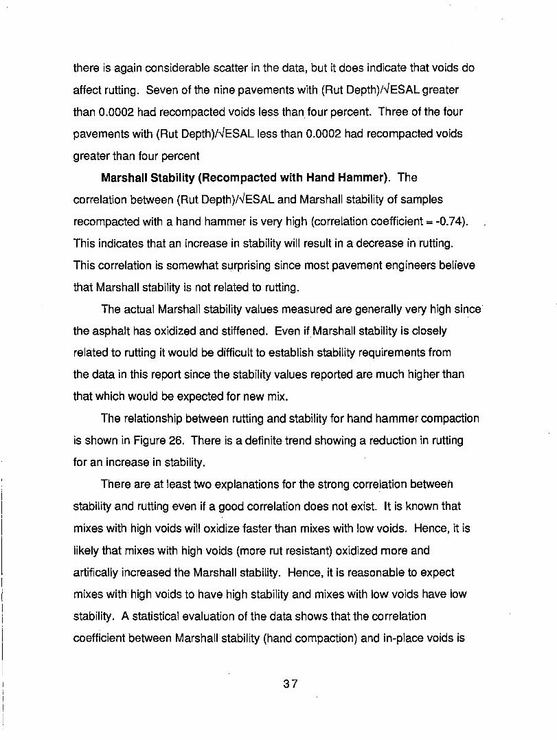
there is again considerable scatter in the data, but it does indicate that voids do
affect rutting. Seven of the nine pavements with (Rut Depth)I..JESAL greater
than 0.0002 had recompacted voids less than four percent. Three of the four
pavements with (Rut Depth)I..JESAL less than 0.0002 had recompacted voids
greater than four percent
Marshall Stability (Recompacted with Hand Hammer). The
correlation between (Rut Depth)I..JESAL and Marshall stability of samples
recompacted with a hand hammer is very high (correlation coefficient = -0.74).
This indicates that an increase in stability will result in a decrease in rutting.
This correlation is somewhat surprising since most pavement engineers believe
that Marshall stability is not related to rutting.
The actual Marshall stability values measured are generally very high since
the asphalt has oxidized and stiffened. Even if Marshall stability is closely
related to rutting it would be difficult to establish stability requirements from
the data in this report since the stability values reported are much higher than
that which would be expected for new mix.
The relationship between rutting and stability for hand hammer compaction
is shown in Figure 26. There is a definite trend showing a reduction in rutting
for an increase in stability.
There are at least two explanations for the strong correlation between
stability and rutting even if a good correlation does not exist. It is known that
mixes with high voids will oxidize faster than mixes with low voids. Hence, it is
likely that mixes with high voids (more rut resistant) oxidized more and
artifically increased the Marshall stability. Hence, it is reasonable to expect
mixes with high voids to have high stability and mixes with low voids have low
stability. A statistical evaluation of the data shows that the correlation
coefficient between Marshall stability (hand compaction) and in-place voids is
37
0.70 and Marshall stability (gyratory compaction) and in-place voids is 0.67.
These high correlations between voids and stability likely explains part of the
reason that rutting and stability appear to be closely correlated.
Another explanation for the good correlation is the way sites were selected
for this project. Those sites with more rutting had generally been in-place a
shorter time than those sites with little rutting. Everything else being equal,
this would result in the least rutted pavements having higher stbility that the
more rutted pavements simply because of pavement age. The older pavements
being more oxidized would have higher stabilities.
Considering the above discussion it is still likely that there exist some
correlation between stability and rutting.
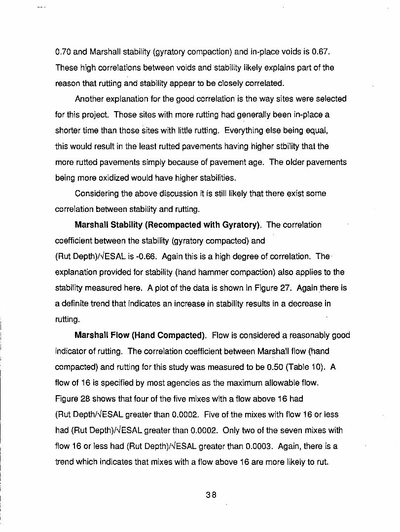
Marshall Stability (Recompacted with Gyratory). The correlation
coefficient between the stability (gyratory compacted) and
(Rut Depth)/--JESAL is -0.66. Again this is a high degree of correlation. The·
explanation provided for stability (hand hammer compaction) also applies to the
stability measured here. A plot of the data is shown in Figure 27. Again there is
a definite trend that indicates an increase in stability results in a decrease in
rutting.
Marshall Flow (Hand Compacted). Flow is considered a reasonably good
indicator of rutting. The correlation coefficient between Marshall flow (hand
compacted) and rutting for this study was measured to be 0.50 (Table 10). A
flow of 16 is specified by most agencies as the maximum allowable flow.
Figure 28 shows that four of the five mixes with a flow above 16 had
(Rut Depth/--JESAL greater than 0.0002. Five of the mixes with flow 16 or less
had (Rut Depth)/--JESAL greater than 0.0002. Only two of the seven mixes with
flow 16 or less had (Rut Depth)/--JESAL greater than 0.0003. Again, there is a
trend which indicates that mixes with a flow above 16 are more likely to rut.
38
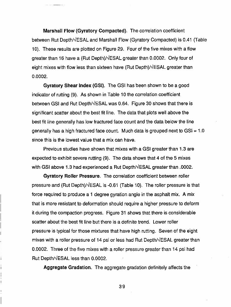
Marshall Flow (Gyratory Compacted). The correlation coefficient
between Rut Depth/"ESAL and Marshall Flow (Gyratory Compacted) is 0.41 (Table
1 0). These results are plotted on Figure 29. Four of the five mixes with a flow
greater than 16 have a (Rut Depth)/"ESAL greater than 0.0002. Only four of
eight mixes with flow less than sixteen have (Rut Depth)/"ESAL greater than
0.0002.
Gyratory Shear Index (GSI). The GSI has been shown to be a good
indicator of rutting (9). As shown in Table 10 the correlation coefficient
between GSI and Rut Depth/"ESAL was 0.64. Figure 30 shows that there is
significant scatter about the best fit line. The data that plots well above the
best fit line generally has low fractured face count and the data below the line
generally has a high fractured face count. Much data is grouped next to GSI = 1:0
since this is the lowest value that a mix can have.
Previous studies have shown that mixes with a GSI greater than 1.3 are
expected to exhibit severe rutting (9). The data shows that 4 of the 5 mixes
with GSI above 1.3 had experienced a Rut Depth/"ESAL greater than .0002.
Gyratory Roller Pressure. The correlation coefficient between roller
pressure and (Rut Depth)/"ESAL is -0.61 (Table 10). The roller pressure is that
force required to produce a 1 degree gyration angle in the asphalt mix. A mix
that is more resistant to deformation should require a higher pressure to deform
it during the compaction progress. Figure 31 shows that there is considerable
scatter about the best fit line but there is a definite trend. Lower roller
pressure is typical for those mixtures that have high rutting. Seven of the eight
mixes with a roller pressure of 14 psi or less had Rut Depth/"ESAL greater than
0.0002. Three of the five mixes with a roller pressure greater than 14 psi had
Rut Depth/"ESAL less than 0.0002.
Aggregate Gradation. The aggregate gradation definitely affects the
39
rutting resistance of an asphalt mixture but this is a difficult property to
analyze. Studies have shown that the maximum aggregate size is important as
well as percent passing No. 200 sieve are important (13,14). However, the
overall evaluation of individual gradations is difficult. For this project the
percent passing 3/8 inch sieve, percent passing No. 50, and percent passing No.
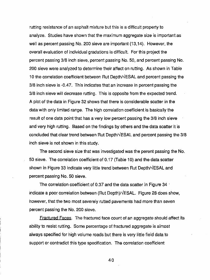
200 sieve were analyzed to determine their affect on rutting. As shown in Table
10 the correlation coefficient between Rut Depth/"ESAL and percent passing the
3/8 inch sieve is -0.47. This indicates that an increase in percent passing the
3/8 inch sieve will decrease rutting. This is opposite from the expected trend.
A plot of the data in Figure 32 shows that there is considerable scatter in the
data with only limited range. The high correlation coefficient is basically the
result of one data point that has a very low percent passing the 3/8 inch sieve
and very high rutting. Based on the findings by others and the data scatter it is
concluded that clear trend between Rut Depth/"ESAL and percent passing the 3/8
inch sieve is not shown in this study.
The second sieve size that was investigated was the perent passing the No.
50 sieve. The correlation coefficient of 0.17 (Table 10) and the data scatter
shown in Figure 33 indicate very little trend between Rut Depth/"ESAL and
percent passing No. 50 sieve.
The correlation coefficient of 0.37 and the data scatter in Figure 34 .
indicate a poor correlation between (Rut Depth)/"ESAL. Figure 28 does show,
however, that the two most severely rutted pavements had more than seven
percent passing the No. 200 sieve.
Fractured Faces. The fractured face count of an aggregate should affect its
ability to resist rutting. Some percentage of fractured aggregate is almost
always specified for high volume roads but there is very little field data to
support or contradict this type specification. The correlation coefficient
40
between fractured face count and (Rut Depth)/ -vESAL for the study was -0.13
(Table 10). This is a very low correlation that shows a slight trend toward less
rutting for higher fractured face count.
The correlation appears to be much better than this after reviewing Figure
35. The two mixes with highest (Rut Depth)/-vESAL (Site 5 = 77.1 x 10⁻⁵ and
Site 8 = 79.2 x 10⁻⁵) also had high fractured face counts (Site 5 = 81.0% and Site
8 = 98.1 %). These mixes had low in-place voids (Site 5 = 2.3% and Site 8 = 0.6%).
Site 5 was the most severely rutted site studied (Rut Depth = 1.09 inches) with
rutting well into plastic flow. Plastic flow had not started at Site 8, but the
mix was characterized by verh high asphalt content (7.8%) and very low in-place
voids (0.6%). If the data for Site 8 is eliminated, for unrealistically high asphalt
content, the correlation coefficient becomes -0.41 indicating a much stronger
trend.
The data in Figure 35 shows that all six mixes with fractured face
percentages of 80 or less had a (Rut Depth/ -vESAL greater than .0002. The data
also shows that four out of seven mixes with a fractured face count greater than
80 had (Rut Depth/ -V ESAL less than .0002, including the two mixes discussed
above.
Fine Aggregate Shape & Texture. Uncompacted voids from the NAA flow
test (12) and time from the modified test measure particle angularity and'
texture. Higher voids and flow times indicate rougher textured and more angular
particles. The correlation coefficients in Table 10 shows that flow time from
the modified NAA test has very little correlation (0.05). Uncompacted voids
from the NAA test have better (0.15), but still very poor correlation.
Figure 36 shows the weak trend for uncompacted voids, but the trend
indicates that an increase in voids will result in an increase in rutting. This is
opposite of the expected trend. It appears from Figure 36 that the data from
41
Sites 5 and 8, which have the two highest rates of rutting, do not follow the
pattern of the data at other sites. If the data point for Site 8 (45.9, 79.2 x 10
-5) is omitted, for unrealistically high asphalt content, the correlation
coefficient becomes -0.25 indicating a stronger trend. More importantly the sign
of the correlation coefficient is reversed and indicates, as expected, that rate of
rutting decreases as uncompacted voids increases.
Figure 37 illustrates the very weak correlation for flow time. Again, if the
data point for Site 8 (23.9, 79.2 x 10 -5) is omitted, the correlation coefficient
becomes - 0.37. This not only represents a dramatic increase in magnitude, but
the change in sign means that the trend is in the expected direction, i.e., rate of
rutting decreases as flow time increases. The performance of the mix at Site 8
demonstrates the multiplicity of factors that can influence rutting performance,
and the importance of both aggregate properties and asphalt content during
material selection and mix design.
Asphalt Penetration. The data in Table 10 shows that the correlation
coefficient between (Rut Depth/..JESAL and penetration is 0.46. The data plotted
in Figure 38 shows an obvious trend indicating an increase in penetration would
result in an increase in rutting. Since most asphalt pavements in Alabama begin
with similar penetration, it is not clear what this trend indicates. As before, it
may be that larger voids result in more oxidation of the asphalt and better'
resistance to rutting. At any rate it is reasonable to expect more rutting when
using an asphalt with higher penetration.
Viscosity. The correlation coefficient between (Rut Depth)I...jESAL and
viscosity is -0.50 as shown in Table 10. The trend is shown graphically in Figure
39. This indicates that an increase in viscosity would result in a decrease in
Rutting. The discussion under asphalt penetration will also be true for viscosity.
Predictive MOdel. In developing a combined predictive model, those
42
properties that were independent of each other that appeared to correlate best
with rutting and those easily measured were selected. After evaluation of
several combinations it was determined that the best combination included the
following three properties: voids in laboratory compacted samples, percent of
fractured faces, and percent of material passing the No. 200 sieve. This model
which has an R2 of 0.35 is shown in Figure 40. The equation can be used to
estimate (Rut Depth/"ESAL) from the three aggregate and mix properties. Mixes
resulting in estimates greater than 0.0002 should be examined carefully for
redesign.
Geographic and Aggregate Property Relationships.
In the section on the analysis of rutting data from the AHD pavement
condition database, it was concluded that pavement rutting susceptibility was
related to geographical area and that variable geology and, thus, variable quality
aggregate was the most probable cause. Specifically it was concluded that
pavements in Divisions 5-9 which are located in the Coastal Plain, where natural
sands and gravels are used, are more susceptible to rutting than pavements in
Divisions 1-4 which are located predominately in the Appalachian Plateau and
Piedmont geologic regions, where crushed stone is available.
Particle shape and texture are assumed to be indicators of aggregate quality
and several parameters will be compared for the extracted aggregates from
Sites 1-4 and 5-6. Average values for the parameters are contained in Table 11.
For the fine aggregate fraction (minus No.8, voids from the NAA test and
flow time from the modified NAA test were compared. Average NAA voids and
flow times are larger for the sites in Divisions 1-4 indicating more angular
particles with rougher surface texture. This was the expected response since
both angularity and surface texture are indirectly related to weathering or
distance transported.
43
Crushed face counts are a measure of particle angularity and were made on
coarse (plus No.8) aggregate particles. These counts can also be used to indicate
angularity of coarser fractions, i.e., plus No.4 particles. The plus No.4 fraction
is considered because AHD specifications for surface mix aggregate have the
requirement that 80% of these particles have two (2) or more crushed faces.
Percentages of particles having two or more crushed faces for the plus No.8 and
plus No.4 fractions are shown in Table 11. The numbers are somewhat different
but both sizes indicate the same differences between the aggregate from sites in
Divisions 1-4 and the aggregate from sites in Divisions 5-9.
For surface mixes the percentages of particles with two or more crushed
faces is only slightly larger in Divisions 1-4 than in Divisions 5-6. This is
probably due to the widespread use of crushed gravel coarse aggregate statewide
with only slightly more granite and slag used in Divisions 1-4.
For binder mixes the percentages in Divisions 1-4 are 100% and
approximately twice those in Divisions 5-6. This si due to the sidespread use of
crushed limestone in Divisions 1-4. For combined mixes the percentages for both
size fractions are larger in Divisions 1-4 than in Divisions 5-6, indicating more
angular course aggregate particles in Divisions 1-4.
44
CONCLUSIONS AND RECOMMENDATIONS
Analyses of the Department's pavement condition database indicate that
rutting in Alabama is increasing, and that this increase is attributible to either
increased loading intensity or increased asphalt concrete rutting susceptibility.
The analyses also indicate that rutting varies geographically and that this
variation can be explained by quality of locally available aggregate. Those areas
with crushed stone and angular natural sands are less susceptible to rutting.
Analyses of data from field test sites indicate that permanent deformation
causing rutting is generally confined to the top 3 to 4 inches (surface and binder
courses). There was little evidence that lower base/subbase courses or subgrade
were significant contributors to rutting. At only one site was there evidence
that stripping may have contributed to rutting. There was some evidence that
surface treatment layers used in conjunction with thin overlays may have
contributed to rutting susceptibility. A rate of rutting of 2 x 10⁻⁴ in/..JESAL or
1.0 x 10⁻⁷ in/ESAL delineated good and poor performing pavements.
The properties measured in this study that appear to be useful in minimizing
rutting include: layer thickness, voids, GSI, Gyratory roller pressure, percent of
fractured faces, percent passing No. 200 sieve, Marshall flow, and creep strain.
The R2 for most of these properties were low, however, there appeared to be a
definite trend shown in the figures. The low R2 in almost every case was caused
by one or two of the data points being far outside the range of the other data.
This shows that rutting is a very complicated process and is affected by a large
number of factors and hence, to use only a small number of properties to
accurately predict rutting is impossible.
The best model selected for predicting rutting had an R2 equal to 0.35 and
included the voids in laboratory compacted samples, percent coarse aggregate
with two or more faces, and percent of materials pasisng the No. 200 sieve.
45
The crushing of gravel should be more carefully controlled to insure that the
800/0 requirement for particles with two fully fractured faces is met. This may
require limitations on minimum particle size for crushing. On heavily traveled
roadways (state primary and interstate routes) crushed particle requirements
for binder mixes should be the same as surface mixes. The use of a test, such as
the National Aggregate Association's uncompacted voids method, to quantify and
limit particle shape and texture of fine aggregate should recieve additional study
but this study showed no correlation.
The use of surface treatment interlayers, particularly in conjunction with
thin overlays, should receive further study. This study should focus 1) on
identifying conditions where surface treatment interlayers should and should not
be used, and 2) on construction control procedures that will prevent excess
asphalt cement that could soften the overlay and increase rutting susceptibility.
Procedures should be adopted for better control of asphalt content during
construction. Target job mix formula asphalt content should not be changed
without sufficient test results to justify changes.
46
1.
2.
3.
4.
5.
6.
7.
8.
9.
10.
11.
12.
References
Middleton, D.R., F.L. Roberts and T. Chira-Chavala, "Measurement and Analysis of Truck Tire Pressures on Texas Highways," in Transportation Research Record 1070, Transportation Research Board, Washington, D.C., 1986, pp. 1-8.
Thompson, M.R., "Analytical Methods for Considering Tire Pressure Effects in Pavement Design," Proceedings, in A SymposiumlWorkshop on High Pressure Truck Tires, American Association of State Highway and Transportation Officials and Federal Highway Administration, Austin, Texas, February 1987.
Kim, O. and C.A. Bell, "Measurement and Analysis of Truck Tire Pressures in Oregon," in Transportation Research Record 1207, Transportation Research Board, Washington, D.C., 1988, pp. 100-110.
Hudson, S.W. and S.B. Seeds, "Evaluation of Increased Pavement Loading and Tire Pressures," in Transportation Research Record 1207, Transportation Research Board, Washington, D.C., 1988, pp. 197-206 .
.......... --;--_~-;-, "High-Pressure Truck Tires," in Pavement Newsletter, Federal Highway Administration, Washington, D.C., January 1988. .
Marshek, K.M., H.H. Chen, R.B. Connell and W.R. Hudson, "Experimental Determination of Pressure Distribution of Truck Tire Pavement Contact," in Transportation Research Record 1070, Transportation Research Board, Washington, D.C., 1986, pp. 9-14.
-=--:-:----:-..----_, "Pavement Condition Survey, Distress Identification and Rating Manual," Bureau of Materials and Tests, Alabama Highway Department, Montgomery, Alabama, July 1988 .
............. ~..-;--=-:==-, "Truck Weights as Related to Pavement Design in Alabama," HPR No. 96, Project No. 930-106, Bureau of Materials and Tests, Alabama Highway Department, Montgomery, Alabama, June 1983.
Brown, E.R. and Stephen A. Cross, "A Study of In-Place Rutting of Asphalt Pavements," Proceedings, Association of Asphalt Paving Technologi.sts, Volume 58, 1989, pp. 1-39.
Ford, M.C., "Pavement Densification Related to Asphalt Mix Characteristics," paper presented at 67th Annual Transportation Research Board Meeting, January 1988.
Huber, G.A. and G.H. Herman, "Effect of Asphalt Concrete Parameters on Rutting Performance: A Field Investigation,' Proceedings, Association of Asphalt Paving Technolgoists, Volume 56, 1987, pp. 33-61.
Meininger, R.C., "Proposed Method of Test for Particle Shape and Texture of Fine Aggregate Using Uncompacted Void Content," National Aggregates Association, Silver Springs, Maryland, March 1989.
47
13.
14.
Brown, E.R., J.L. McRae and A. Crawley, "Effect of Aggregate on Performance of Bituminous Concrete," Implication of Aggregate in the Design, Construction, and Performance of Flexible Pavement, ASTM Special Technical Publication 1016, Schreuders and Marek, ASTM, 1989, pp. 34-63.
Brown, E.R. and Charles E. Bassett, "The Effects of Maximum Aggregate Size on Rutting Potential and other Properties of Asphalt-Aggregate Mixture," Paper presented at TRB Meeting, January 1990.
48

TABLES
49 .
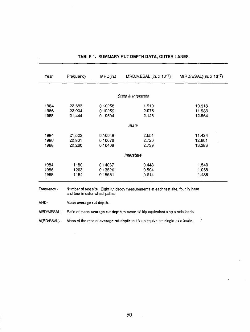
TABLE 1. SUMMARY RUT DEPTH DATA, OUTER LANES
Year Frequency MRD(in.) MRD/MESAL (in. x 10-7) M(RD/ESAL)(in. x 10-7)
State & Interstate
1984 22,683 0.10258 1.919 10.918 1986 22,004 0.10259 2.076 11.983 1988 21,444 0.10694 2.123 12.564
State
1984 21,503 0.10049 2.551 11.424 1986 20,801 0.10070 2.720 12.601 1988 20,260 0.10409 2.739 13.283
Interstate
1984 1180 0.14067 0.448 1.540 1986 1203 0.13526 0.504 1.068 1988 1184 0.15561 0.614 1.488
Frequency - Number of test site. Eight rut depth measurements at each test site, four in inner and four in outer wheel paths.
MRD- Mean average rut depth.
MRDIMESAL- Ratio of mean average rut depth to mean 18 kip equivalent single axle loads.
M(RD/ESAL) - Mean of the ratio of average rut depth to 18 kip equivalent single axle loads.
50
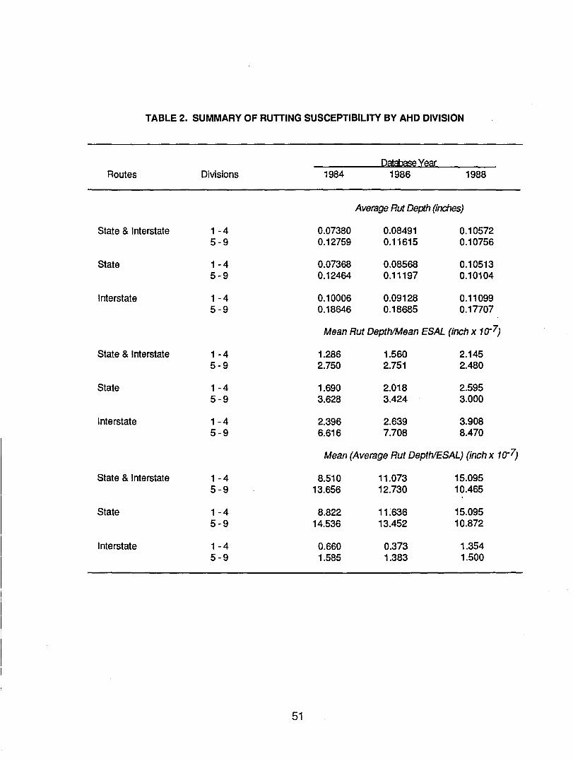
TABLE 2. SUMMARY OF RUTTING SUSCEPTIBILITY BY AHD DIVISION
Qata~YeS[ Routes Divisions 1984 1986 1988
Average Rut Depth (inches)
State & Interstate 1 -4 0.07380 0.08491 0.10572 5-9 0.12759 0.11615 0.10756
State 1 - 4 0.07368 0.08568 0.10513 5-9 0.12464 0.11197 0.10104
Interstate 1-4 0.10006 0.09128 0.11099 5-9 0.18646 0.18685 0.17707
Mean Rut Depth/Mean ESAL (inch x 10-7)
State & Interstate 1-4 1.286 1.560 2.145 5-9 2.750 2.751 2.480
State 1 -4 1.690 2.018 2.595 5-9 3.628 3.424 3.000
Interstate 1-4 2.396 2.639 3.908 5-9 6.616 7.708 8.470
Mean (Average Rut Depth/ESAL) (inch x 10-7)
State & Interstate 1-4 8.510 11.073 15.095 5-9 13.656 12.730 10.465
State 1-4 8.822 11:636 15.095 5-9 14.536 13.452 10.872
Interstate 1-4 0.660 0.373 1.354 5-9 1.585 1.383 1.500
51
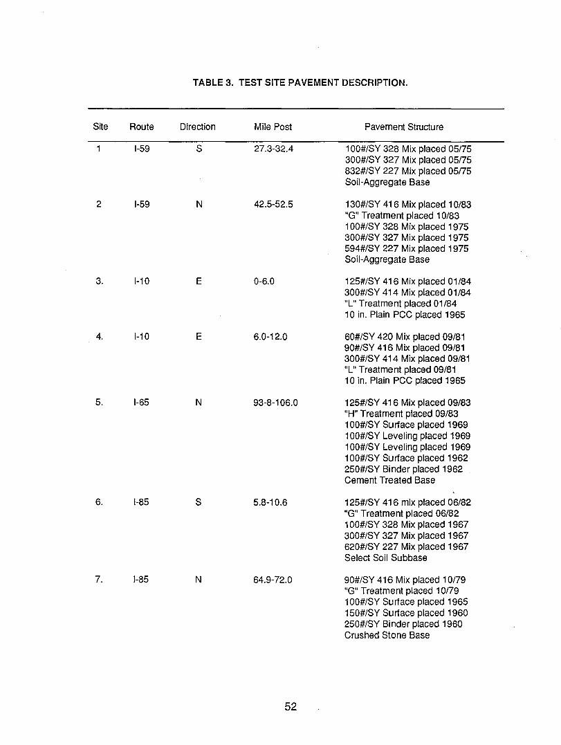
TABLE 3. TEST SITE PAVEMENT DESCRIPTION.
Site Route Direction Mile Post Pavement Structure
1 I-59 S 27.3-32.4 1 OO#/SY 328 Mix placed 05/75 300#/SY 327 Mix placed 05175 832#/SY 227 Mix placed 05175 Soil-Aggregate Base
2 I-59 N 42.5-52.5 130#/SY 416 Mix placed 10/83 "G" Treatment placed 1 0/83 1 OO#/SY 328 Mix placed 1975 300#/SY 327 Mix placed 1975 594#/SY 227 Mix placed 1975 SOil-Aggregate Base
3. 1-10 E 0-6.0 125#/SY 416 Mix placed 01/84 300#/SY 414 Mix placed 01/84 "L" Treatment placed 01/84 1 0 in. Plain PCC placed 1965
4. 1-10 E 6.0-12.0 60#/SY 420 Mix placed 09/81 90#/SY 416 Mix placed 09/81 300#/SY 414 Mix placed 09/81 "L" Treatment placed 09/81 1 0 in. Plain PCC placed 1965
5. 1-65 N 93-8-106.0 125#/SY 416 Mix placed 09/83 "H" Treatment placed 09/83 1 OO#/SY Suriace placed 1969 100#/SY Leveling placed 1969 100#/SY Leveling placed 1969 100#/SY Suriace placed 1962 250#/SY Bi nder placed 1962 Cement Treated Base
6. 1-85 S 5.8-10.6 125#/SY 416 mix placed 06/82 "G" Treatment placed 06/82 1 OO#/SY 328 Mix placed 1967 300#/SY 327 Mix placed 1967 620#/SY 227 Mix placed 1967 Select Soil Subbase
7. 1-85 N 64.9-72.0 90#/SY 416 Mix placed 1 0/79 "G" Treatment placed 1 0/79 1 OO#/SY Suriace placed 1965 150#/SY Suriace placed 1960 250#/SY Binder placed 1960 Crushed Stone Base
52
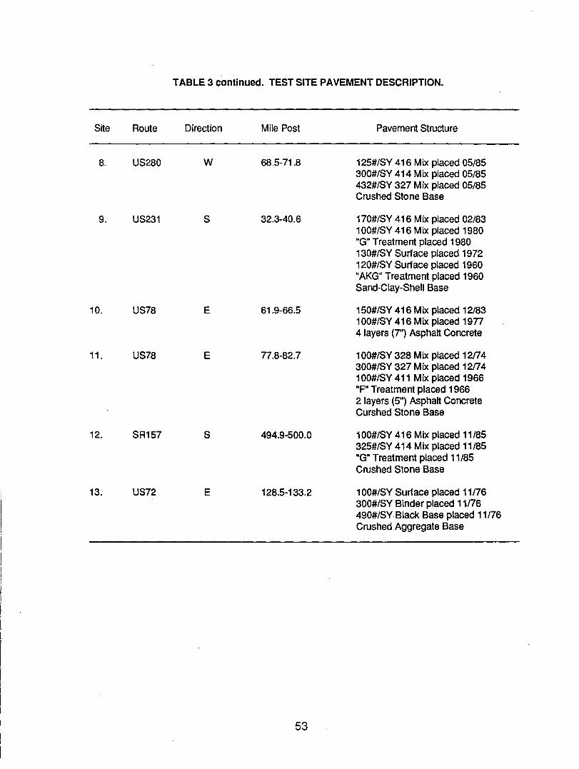
TABLE 3 continued. TEST SITE PAVEMENT DESCRIPTION.
Site Route Direction Mile Post Pavement Structure
8. US280 W 68.5-71.8 125#/SY 416 Mix placed 05/85 300#/SY 414 Mix placed 05/85 432#/SY 327 Mix placed 05/85 Crushed Stone Base
9. US231 S 32.3-40.6 170#/SY 416 Mix placed 02/83 100#/SY 416 Mix placed 1980 "G" Treatment placed 1980 130#/SY Surface placed 1972 120#/SY Surface placed 1960 "AKG" Treatment placed 1960 Sand-Clay-Shell Base
10. US78 E 61.9-66.5 150#/SY 416 Mix placed 12/83 100#/SY 416 Mix placed 1977 4 layers (7") Asphalt Concrete
11. US78 E 77.8-82.7 100#/SY 328 Mix placed 1204 300#/SY 327 Mix placed 1204 1 OO#/SY 411 Mix placed 1966 "F" Treatment placed 1966 2 layers (5") Asphalt Concrete Curshed Stone Base
12. SR157 S 494.9-500.0 100#/SY 416 Mix placed 11/85 325#/SY 414 Mix placed 11/85 "G" Treatment placed 11/85 Crushed Stone Base
13. US72 E 128.5-133.2 100#/SY Surface placed 11/76 300#/SY Binder placed 1106 490#/SV.Black Base placed 11/76 Crushed Aggregate Base
53
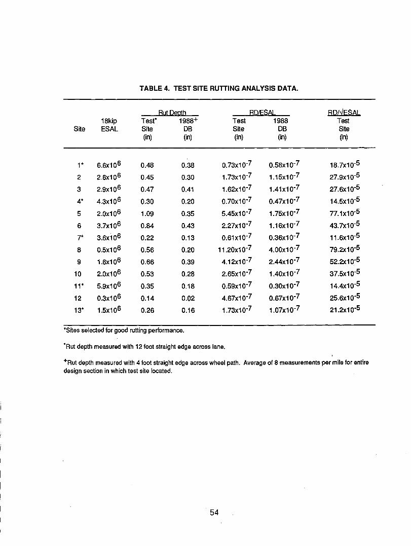
TABLE 4. TEST SITE RUTTING ANALYSIS DATA.
But Dej;llb BDIESAL BOdESAL. 18kip Test" 1988+ Test 1988 Test
Site ESAL Site DB Site DB Site (in) (in) (in) (in) (in)
1* 6.6x106 0.48 0.38 0.73x10⁻⁷ 0.S8x10-7 18.7x10-S
2 2.6x10⁶ O.4S 0.30 1.73x10⁻⁷ 1.1Sx10-7 27.9x10-S
3 2.9x10⁶ 0.47 0.41 1.62x10⁻⁷ 1.41x10⁻⁷ 27.6x10-S
4* 4.3x106 0.30 0.20 0.70x10⁻⁷ 0.47x10⁻⁷ 14.Sx10-S
S 2.0x10⁶ 1.09 0.3S S.4Sx10-7 1.7Sx10-7 77.1x10-S
6 3.7x10⁶ 0.84 0.43 2.27x10⁻⁷ 1.16x10⁻⁷ 43.7x10-S
7* 3.6x106 0.22 0.13 0.61x10⁻⁷ 0.36x10⁻⁷ 11.6x10-S
8 0.Sx106 0.S6 0.20 11.20x10⁻⁷ 4.00x10⁻⁷ 79.2x10-S
9 1.6x10⁶ 0.66 0.39 4.12x10⁻⁷ 2.44x10⁻⁷ S2.2x10-S
10 2.0x10⁶ 0.S3 0.28 2.6Sx10-7 1.40x10⁻⁷ 37.Sx10-S
11* S.9x106 0.3S 0.18 0.S9x10-7 0,30x10⁻⁷ 14.4x10-S
12 0.3x10⁶ 0.14 0.02 4.67x10⁻⁷ 0.67x10⁻⁷ 2S.6x10-S
13* 1.Sx106 0.26 0.16 1.73x10⁻⁷ 1.07x10⁻⁷ 21.2x10-S
·Sites selected for good rutting performance.
"Rut depth measured with 12 foot straight edge across lane.
+Rut depth measured with 4 foot straight edge across wheel path. Average of 8 measurements per mile for entire design section in which test site located.
54
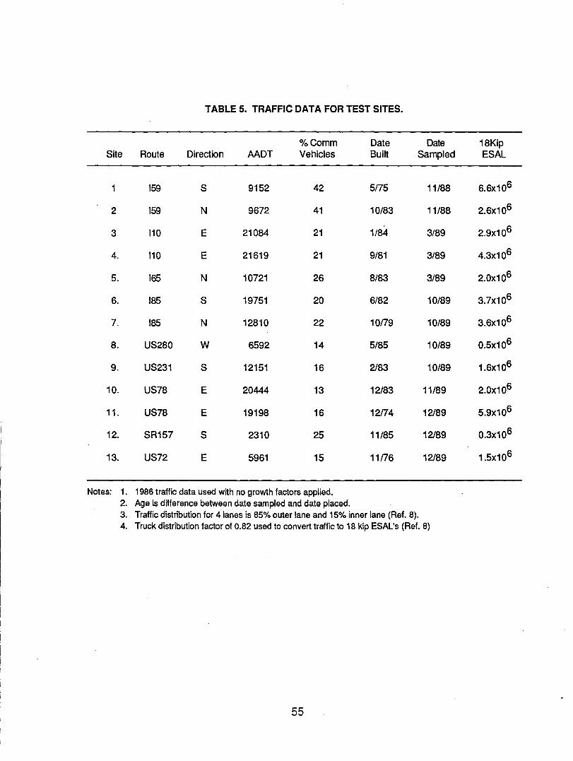
TABLE 5. TRAFFIC DATA FOR TEST SITES.
%Comm Date Date 18Kip Site Route Direction MDT Vehicles Built Sampled ESAL
1 159 S 9152 42 5/75 11/88 6.6x10⁶
2 159 N 9672 41 10/83 11/88 2.6x10⁶
3 110 E 21084 21 1/84 3/89 2.9x10⁶
4. 110 E 21619 21 9/81 3/89 4.3x10⁶
5. 165 N 10721 26 8/83 3/89 2.0x10⁶
6. 185 S 19751 20 6/82 10/89 3.7x10⁶
7. 185 N 12810 22 10179 10/89 3.6x10⁶
8. US280 W 6592 14 5/85 10/89 0.5x10⁶
9. US231 S 12151 16 2/83 10/89 1.6x10⁶
10. US78 E 20444 13 12/83 11/89 2.0x10⁶
11. US78 E 19198 16 12174 12/89 5.9x10⁶
12. SR157 S 2310 25 11/85 12/89 0.3x10⁶
13. US72 E 5961 15 11176 12/89 1.5x10⁶
Notes: 1. 1986 traffic data used with no growth factors applied. 2. Age is dnference between date sampled and date placed. 3. Traffic distribution for 4 lanes is 85% outer lane and 15% inner lane (Ref. 8). 4. Truck distribution factor of 0.82 used to convert traffic to 18 kip ESAL's (Ref. 8)
55
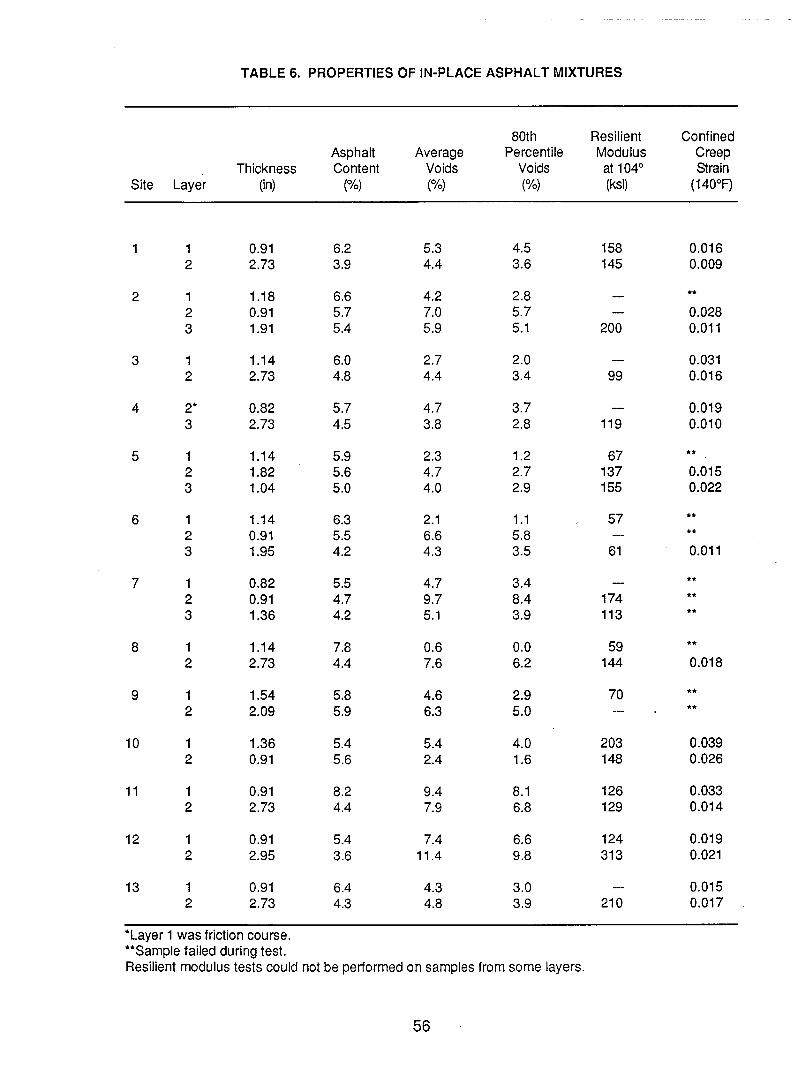
TABLE 6. PROPERTIES OF IN-PLACE ASPHALT MIXTURES
Site Layer
1 1 2
2 1 2 3
3 1 2
4 2· 3
5 1 2 3
6 1 2 3
7 1 2 3
8 1 2
9 1 2
10 1 2
11 1 2
12 1 2
13 1 2
Thickness (in)
0.91 2.73
1.18 0.91 1.91
1.14 2.73
0.82 2.73
1.14 1.82 1.04
1.14 0.91 1.95
0.82 0.91 1.36
1.14 2.73
1.54 2.09
1.36 0.91
0.91 2.73
0.91 2.95
0.91 2.73
*Layer 1 was friction course. ·*Sample failed during test.
Asphalt Content
(%)
6.2 3.9
6.6 5.7 5.4
6.0 4.8
5.7 4.5
5.9 5.6 5.0
6.3 5.5 4.2
5.5 4.7 4.2
7.8 4.4
5.8 5.9
5.4 5.6
8.2 4.4
5.4 3.6
6.4 4.3
Average Voids (%)
5.3 4.4
4.2 7.0 5.9
2.7 4.4
4.7 3.8
2.3 4.7 4.0
2.1 6.6 4.3
4.7 9.7 5.1
0.6 7.6
4.6 6.3
5.4 2.4
9.4 7.9
7.4 11.4
4.3 4.8
80th Percentile
Voids (%)
4.5 3.6
2.8 5.7 5.1
2.0 3.4
3.7 2.8
1.2 2.7 2.9
1.1 5.8 3.5
3.4 8.4 3.9
0.0 6.2
2.9 5.0
4.0 1.6
8.1 6.8
6.6 9.8
3.0 3.9
Resilient modulus tests could not be performed on samples from some layers.
56
Resilient Modulus at 1040
(ksi)
158 145
200
99
119
67 137 155
57
61
174 113
59 144
70
203 148
126 129
124 313
210
Confined Creep Strain
(140°F)
0.016 0.009
•• 0.028 0.011
0.031 0.016
0.019 0.010
** 0.015 0.022
** .*
0.011
** ** **
.*
0.018
*.
**
0.039 0.026
0.033 0.014
0.019 0.021
0.015 0.017
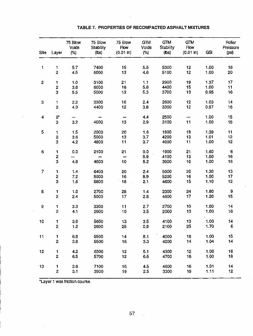
TABLE 7. PROPERTIES OF RECOMPACTED ASPHALT MIXTURES
75 Blow 75 Blow 75 Blow GTM GTM GTM Roller Voids Stability Flow Voids Stability Flow Pressure
Site Layer (%) (Ibs) (0.01 in) (%) (Ibs) (0.01 in) GSI (psQ
1 1 5.7 7400 15 5.5 5300 12 1.00 18 2 4.5 6000 13 4.6 5100 12 1.00 20
2 1 1.0 3100 21 1.1 2900 19 1.37 17 2 3.6 6000 16 5.6 4400 15 1.00 11 3 5.5 5000 13 5.3 3700 13 0.95 16
3 1 2.2 3300 16 2.4 2600 12 1.03 14 2 4.0 4400 12 3.8 3300 12 0.97 16
4 2* 4.4 2500 1.00 15 3 3.2 4000 13 2.9 3100 11 1.00 15
5 1 1.5 2000 20 1.6 1800 18 1.39 11 2 3.6 5000 13 3.7 4200 13 1.01 12 3 4.2 4800 11 3.7 4000 11 1.00 12
6 1 0.0 2100 21 0.0 1900 21 1.60 6 2 5.9 4100 13 1.00 16 3 4.8 4600 10 5.2 3000 10 1.00 16
7 1 1.4 6400 20 2.4 5000 20 1.30 13 2 7.2 8000 16 8.9 5200 16 1.00 17 3 1.6 5800 18 2.1 4600 15 1.10 12
8 1 1.0 2700 28 1.4 2300 24 1.80 9 2 2.4 5000 17 2.8 4600 17 1.20 15
9 1 3.3 3300 11 2.7 2700 10 1.00 14 2 4.1 2600 10 3.5 2000 10 1.00 16
10 1 3.0 5600 13 3.5 4100· 13 1.00 14 2 1.2 2600 25 0.8 2100 25 1.70 6
11 1 6.8 5500 14 8.1 4000 16 1.00 15 2 3.8 5500 16 3.3 4200 14 1.04 14
12 1 4.2 6300 12 5.1 4300 12 1.00 16 2 6.5 5700 12 6.5 4700 16 1.00 18
13 1 2.6 7100 16 4.5 4600 16 1.01 14 2 3.1 3900 19 2.5 3300 19 1.11 12
*Layer 1 was friction course.
57
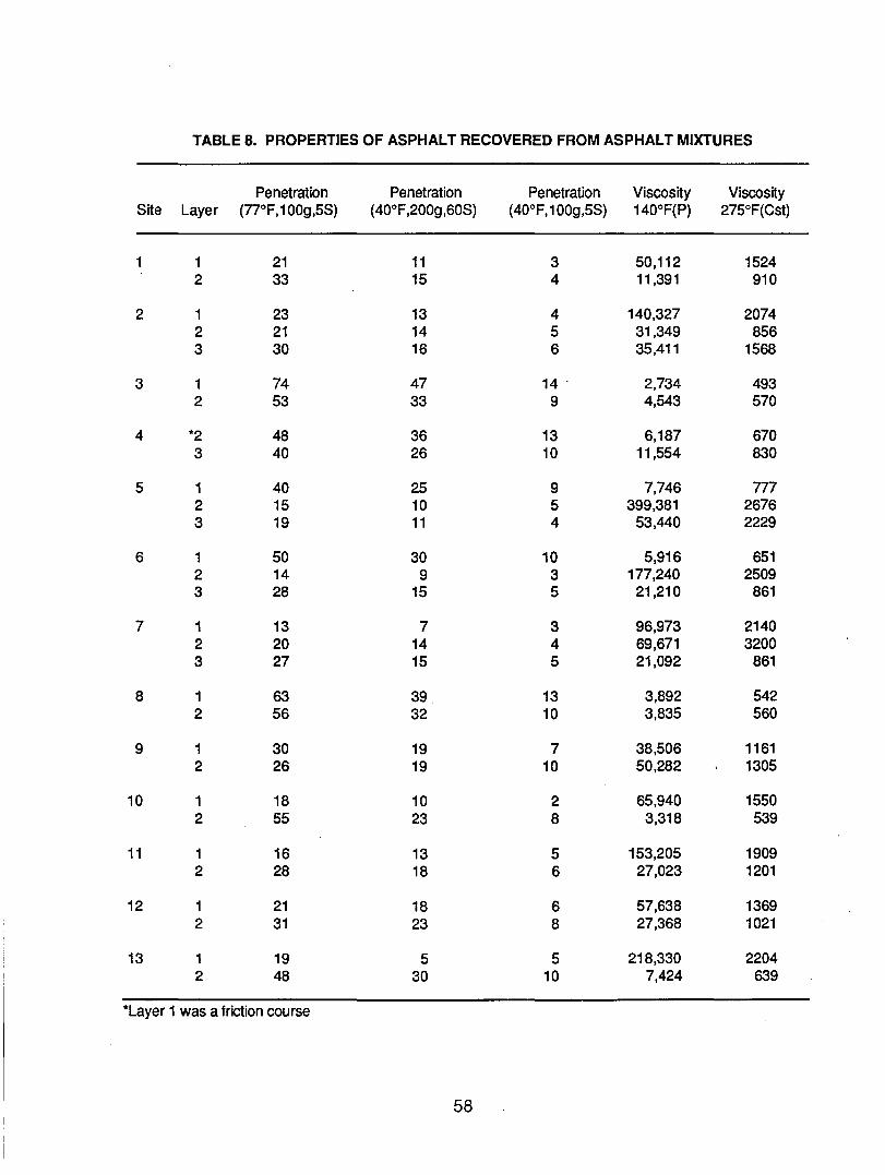
TABLE 8. PROPERTIES OF ASPHALT RECOVERED FROM ASPHALT MIXTURES
Penetration Penetration Penetration Viscosity Viscosny Site Layer (77°F,100g,58) (40°F ,200g ,608) (40°F,100g,58) 140°F(P) 275°F(Cst)
1 1 21 11 3 50,112 1524 2 33 15 4 11,391 910
2 1 23 13 4 140,327 2074 2 21 14 5 31,349 856 3 30 16 6 35,411 1568
3 1 74 47 14 . 2,734 493 2 53 33 9 4,543 570
4 ·2 48 36 13 6,187 670 3 40 26 10 11,554 830
5 1 40 25 9 7,746 777 2 15 10 5 399,381 2676 3 19 11 4 53,440 2229
6 1 50 30 10 5,916 651 2 14 9 3 177,240 2509 3 28 15 5 21,210 861
7 1 13 7 3 96,973 2140 2 20 14 4 69,671 3200 3 27 15 5 21,092 861
8 1 63 39 13 3,892 542 2 56 32 10 3,835 560
9 1 30 19 7 38,506 1161 2 26 19 10 50,282 1305
10 1 18 10 2 65,940 1550 2 55 23 8 3,318 539
11 1 16 13 5 153,205 1909 2 28 18 6 27,023 1201
12 1 21 18 6 57,638 1369 2 31 23 8 27,368 1021
13 1 19 5 5 218,330 2204 2 48 30 10 7,424 639
·Layer 1 was a friction course
58
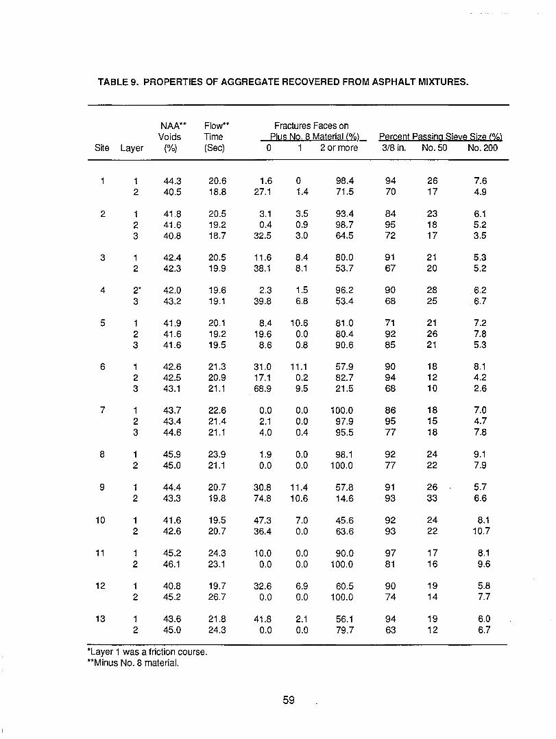
TABLE 9. PROPERTIES OF AGGREGATE RECOVERED FROM ASPHALT MIXTURES.
NAA** Flow** Fractures Faces on Voids Time Plus NQ. a Material (o.(QL PerQent PaSSing Sieve Size (°.(12)
Sne Layer (%) (Sec) 0 1 2 or more 3/8 in. No. 50 No. 200
1 44.3 20.6 1.6 0 98.4 94 26 7.6 2 40.5 18.8 27.1 1.4 71.5 70 17 4.9
2 1 41.8 20.5 3.1 3.5 93.4 84 23 6.1 2 41.6 19.2 0.4 0.9 98.7 95 18 5.2 3 40.8 18.7 32.5 3.0 64.5 72 17 3.5
3 1 42.4 20.5 11.6 8.4 80.0 91 21 5.3 2 42.3 19.9 38.1 8.1 53.7 67 20 5.2
4 2* 42.0 19.6 2.3 1.5 96.2 90 28 6.2 3 43.2 19.1 39.8 6.8 53.4 68 25 .. 6.7
5 1 41.9 20.1 8.4 10.6 81.0 71 21 7.2 2 41.6 19.2 19.6 0.0 80.4 92 26 7.8 3 41.6 19.5 8.6 0.8 90.6 85 21 5.3
6 1 42.6 21.3 31.0 11.1 57.9 90 18 8.1 2 42.5 20.9 17.1 0.2 82.7 94 12 4.2 3 43.1 21.1 68.9 9.5 21.5 68 10 2.6
7 1 43.7 22.6 0.0 0.0 100.0 86 18 7.0 2 43.4 21.4 2.1 0.0 97.9 95 15 4.7 3 44.6 21.1 4.0 0.4 95.5 77 18 7.8
8 1 45.9 23.9 1.9 0.0 98.1 92 24 9.1 2 45.0 21.1 0.0 0.0 100.0 77 22 7.9
9 1 44.4 20.7 30.8 11.4 57.8 91 26 5.7 2 43.3 19.8 74.8 10.6 14.6 93 33 6.6
10 1 41.6 19.5 47.3 7.0 45.6 92 24 8.1 2 42.6 20.7 36.4 0.0 63.6 93 22 10.7
11 1 45.2 24.3 10.0 0.0 90.0 97 17 8.1 2 46.1 23.1 0.0 0.0 100.0 81 16 9.6
12 1 40.8 19.7 32.6 6.9 60.5 90 19 5.8 2 45.2 26.7 0.0 0.0 100.0 74 14 7.7
13 1 43.6 21.8 41.8 2.1 56.1 94 19 6.0 2 45.0 24.3 0.0 0.0 79.7 63 12 6.7
*Layer 1 was a friction course. **Minus NO.8 material.
59
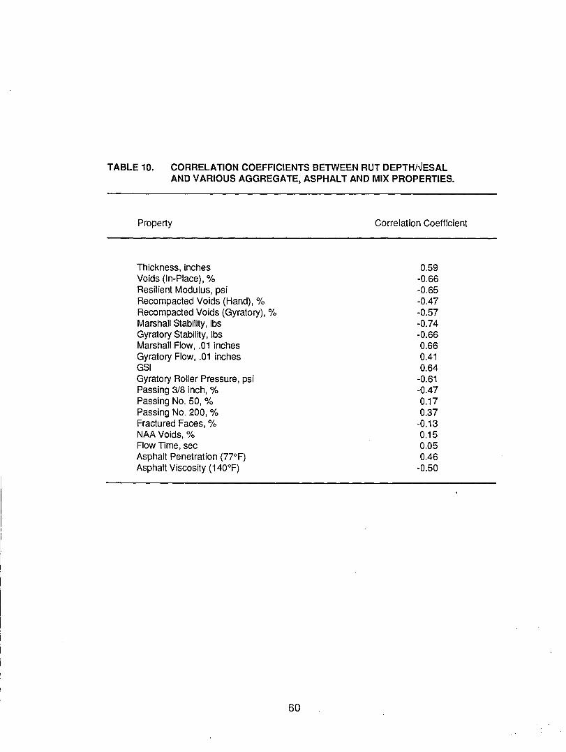
TABLE 10. CORRELATION COEFFICIENTS BETWEEN RUT DEPTH/-vESAL AND VARIOUS AGGREGATE, ASPHALT AND MIX PROPERTIES.
Property
Thickness, inches Voids (In-Place), % Resilient Modulus, psi Recompacted Voids (Hand), % Recompacted Voids (Gyratory), % Marshall Stability, Ibs Gyratory Stability, Ibs Marshall Flow, .01 inches Gyratory Flow, .01 inches GSI Gyratory Roller Pressure, psi Passing 3/8 inch, % Passing No. 50, % Passing No. 200, % Fractured Faces, % NAAVoids, % Flow Time, sec Asphalt Penetration (77°F) Asphalt Viscosity (140°F)
60
Correlation Coefficient
0.59 -0.66 -0.65 -0.47 -0.57 -0.74 -0.66 0.66 0.41 0.64
-0.61 -0.47 0.17 0.37
-0.13 0.15 0.05 0.46
-0.50
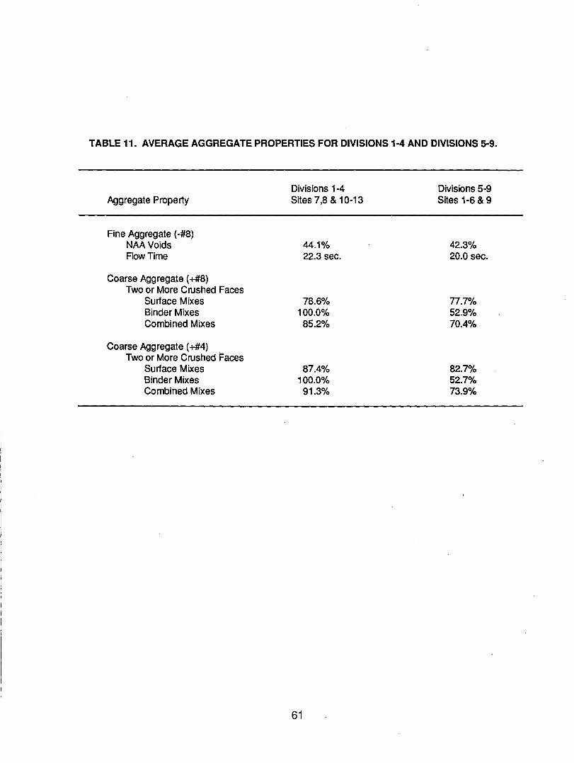
TABLE 11. AVERAGE AGGREGATE PROPERTIES FOR DIVISIONS 1·4 AND DIVISIONS 5-9.
Divisions 1-4 Divisions 5-9 Aggregate Property Sites 7,8 & 10-13 Sites 1-6 & 9
Fine Aggregate (-#8) NAA Voids 44.1'% 42.3% Flow Time 22.3 sec. 20.0 sec.
Coarse Aggregate (+#8) Two or More Crushed Faces
Surface Mixes 78.6% 77.7% Binder Mixes 100.0% 52.9% Combined Mixes 85.2% 70.4%
Coarse Aggregate (+#4) Two or More Crushed Faces
Surface Mixes 87.4% 82.7% Binder Mixes 100.0% 52.7% Combined Mixes 91.3% 73.9%
61

FIGURES
/62 .
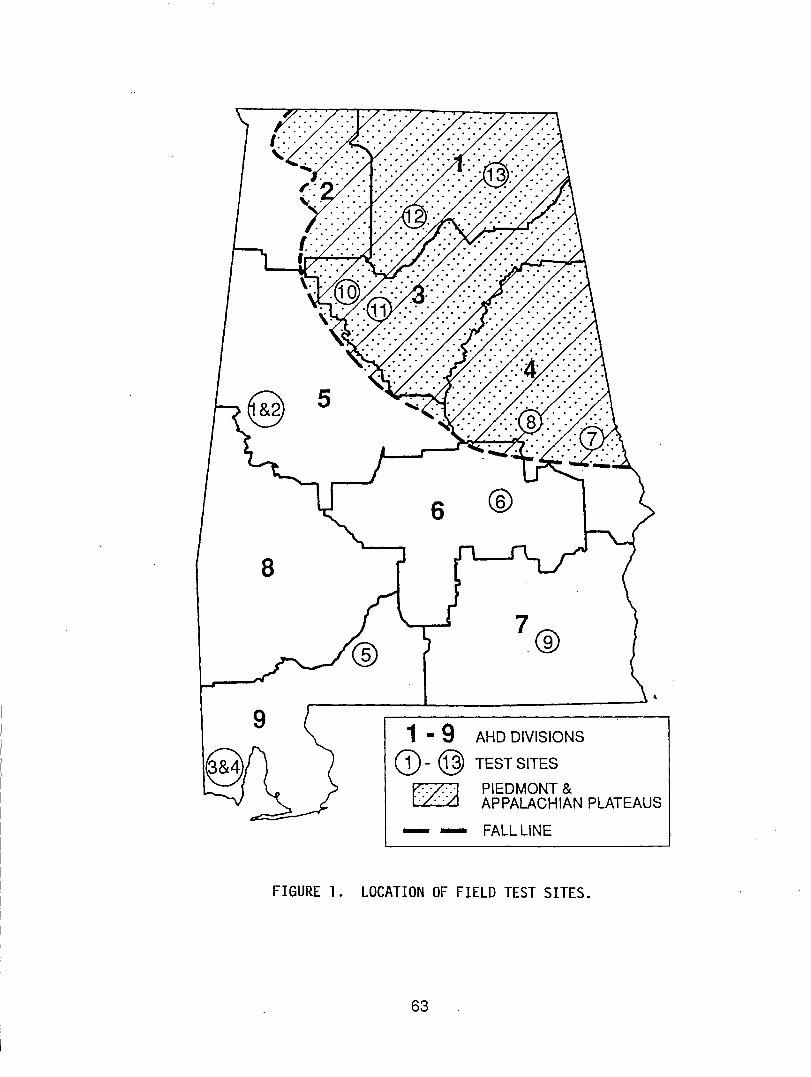
1 - 9 AHD DIVISIONS
CD -@ TEST SITES
r7'l PIEDMONT & l.L.:.LJ APPALACHIAN PLATEAUS
- - FALLLlNE
FIGURE 1. LOCATION OF FIELD TEST SITES.
63
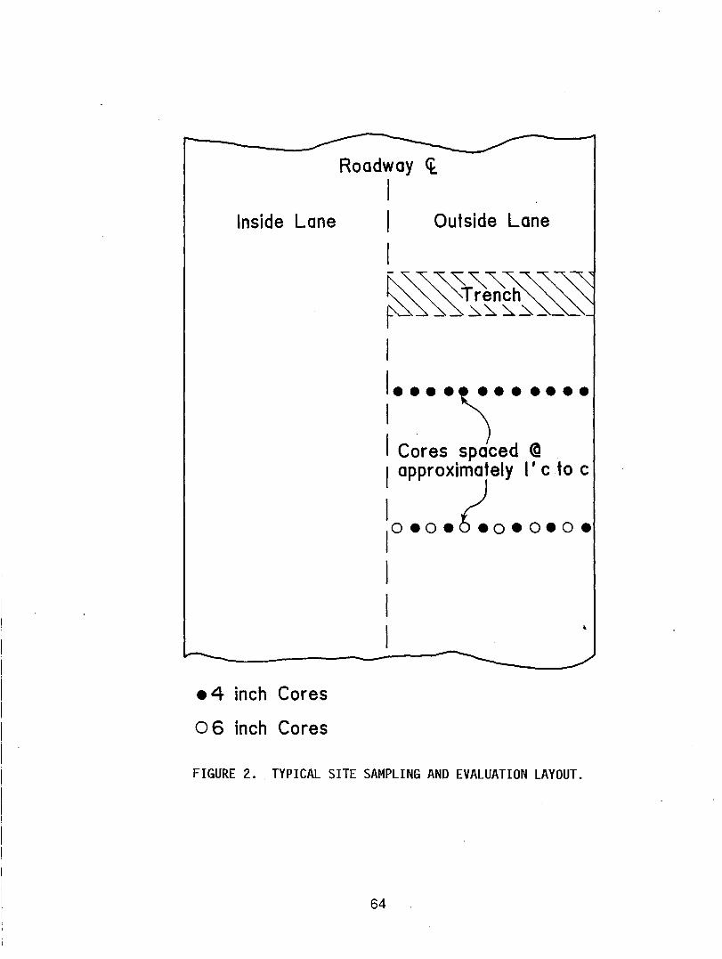
Roadway ~
I Inside Lane I Outside Lane
.4 inch Cores
06 inch Cores
I -~~~~~~~~~ ~~~~~~~ I : .... ~ .. ... . I Cores spaced <a I approximately I' c toc
:0.0.1.0.0.0. I I I
FIGURE 2 .. TYPICAL SITE SAMPLING AND EVALUATION LAYOUT.
64
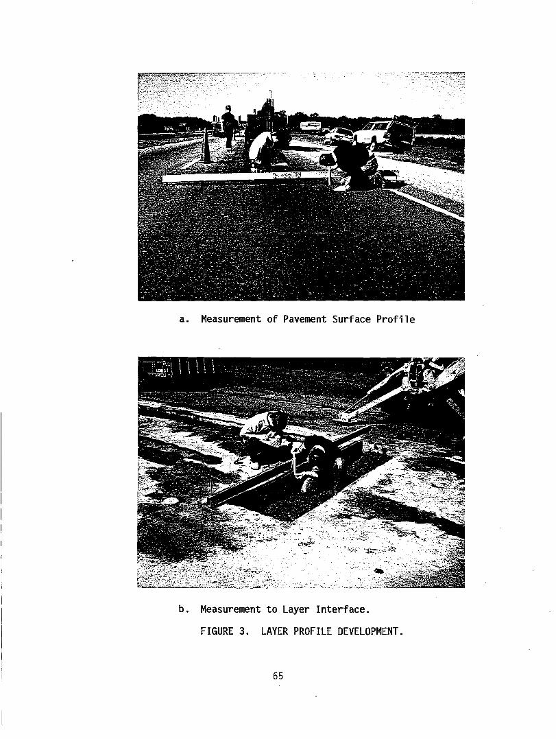
a. Measurement of Pavement Surface Profile
b. Measurement to Layer Interface.
FIGURE 3. LAYER PROFILE DEVELOPMENT.
65
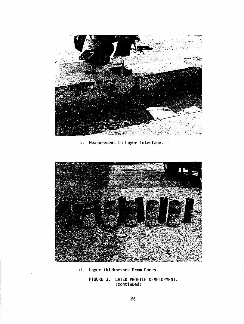
c. Measurement to Layer Interface.
d. Layer Thicknesses From Cores.
FIGURE 3. LAYER PROFILE DEVELOPMENT. (continued)
66
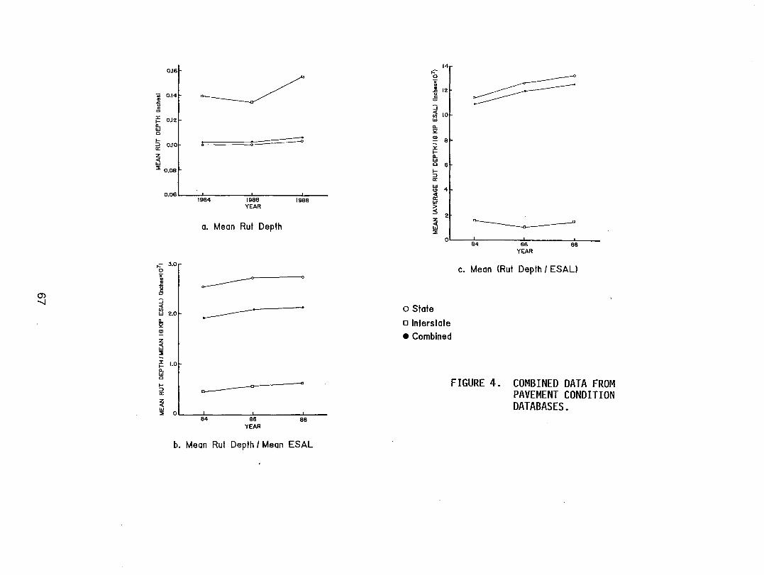
(J) -.....J
0.16
.. 0.14 1 g '" i= OJ2 fu a
~ OJO a: z ~ ~ 0.08
~ ~ --<>
0.06" , I
,:- 3.0 o x .. ., ti §
:J <t 13 2.0
!!. '" <D
Z
~ ~
i= 1.0 n. w a l-
ii! ~ w
1984 1986 1968 YEAR
a. Mean Rut Depth
~
--------~
~ Oll----~8~4~----------~86~-----------8~8=------
YEAR
b. Meon Rut Depth I Meon ESAL
,:o x co
14
~ 12 u c '" :J ~ 10 w !!.
'" <D - 8 J: l-n. w a 6 l-
ii! w C!) 4 <t ffi > ~ z 2
~ ~
~
~ 0' I , ,
o State
o Interstate
• Combined
84 86 88 YEAR
c. Mean (Rut Depth I ESAU
FIGURE 4. COMBINED DATA FROM PAVEMENT CONDITION DATABASES.
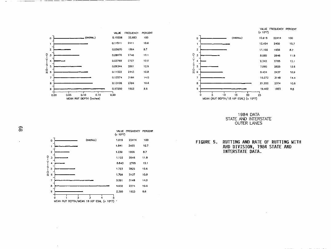
VM..UE FREQUENCY PERCENT
o I (C1VER.'U.) 0.10258 22.683 100
0.11511 2411 10.6
2 0.05670 1964 8.7 -
D 3 I
0.08570 2746 12.1
V 4 I ~
0.03769 2727 12.0
S 5 I 0.09344 2861 12.6
0 N 6 0.11522 2443 10.8
7 0.12574 3184 14.0
8 0.13106 2394 10.6
9 0.17250 1953 B.6
0.00 0.05 0.10 0.15 0.20 MEAN RUT DEPTH (inches)
0') CO VM..UE FREQUENCY PERCENT
(x 10"7)
OJ (C1VER.'U.) 1.919 22414 100
1.941 2400 10.7
2 1.239 1956 8.7
D 3 I
1.122 2646 I1.B
Y 4 ~ 0.843 2705 12.1
T 5 1.723 2825 12.6
0 N 6 1.709 2437 10.9
7 3.291 3148 14.0
8 4.632 2374 10.6
9 2.395 1923 8.6
0 1 2 3 4 5 MEAN RUT DEPTH/MEAN 18 KIP ESM.. (x 10"7)
0
2
D 3 I
Y 4
T 5 0 N 6
7
8
9
VM..UE FREQUENCY PERCENT (x 10"7)
-
0.918
12.424
11.190
8.0B5
2.342
7.560
9.434
10.272
21.552
19.462
o 5 10 15 20 25 MEAN (RUT DEPTH/18 KIP ES/>J...) (x 10"7)
1984 DATA STATE AND INTERSTATE
OUTER LANES
22414 100
2400 10.7
1956 8.7
2646 11.8
2705 12.1
2B25 12.6
2437 10.9
3148 14.4
2374 10.6
1923 8.~
FIGURE 5. RUTTING AND RATE OF RUTTING WITH AHD DIVISION, 1984 STATE AND INTERSTATE DATA.
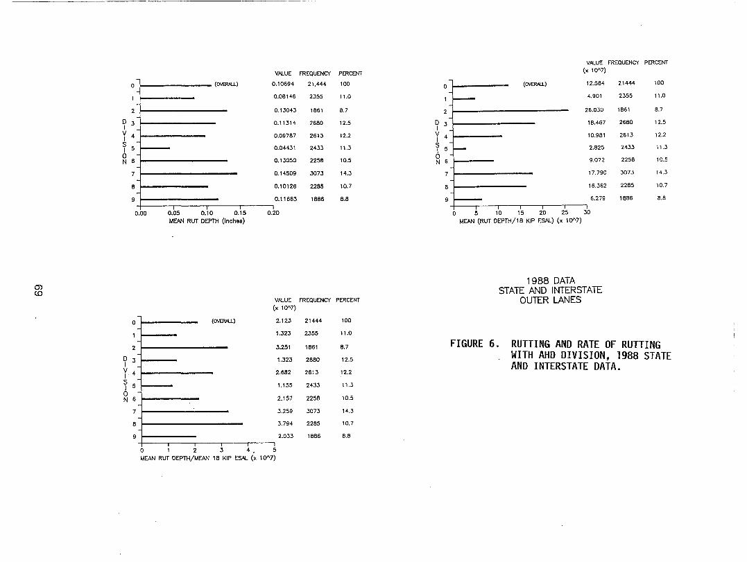
m CD
o
2
D 3 I
Y 4 S 5 I
2 6
7
B
9
~~-VALUE FREQUENCY
.10694
0.08146
21.444
2355
0.13043 lB61
0.11314 26BO
0.097B7 2613
0.04431 2433
0.1 3050 225B
0.14509 3073
0.10126 22B5
0.11663 lBB6
PERCENT
100
11.0
B.7
12.5
12.2
11.3
10.5
14.3
10.7
B.8
0.00 0.05 0.10 0.15 MEAN RUT DEPTH (Inches)
0.20
o
2
D 3 I
Y 4
T 5
2 6
7
8
9
VALUE FREQUENCY PERCENT (x 10"7)
(O'VER.'LL) 2.123
1.323
3.251
1.323
2.6B2
1 1 o 1 2 3 4, 5 MEAN RUT DEPTH/MEAN lB KIP ESAL (x 10"7)
1.155
2.157
3.259
3.794
2.033
21444 100
2355 11.0
lB61 B.7
26BO 12.5
2613 12.2
2433 11.3
225B 10.5
3073 14.3
2285 10.7
lBB6 B.B
0
2
D 3 I
Y 4
T 5 0 N 6
7
8
9
VALUE FREQUENCY PERCENT (x 10"7)
(OVER.AlI.)
I--
I--
2.564
4.901
6.030
1 B.467
10.9Bl
2.B25
9.072
17.790
16.362
6.279
o 5 10 15 20 25 30 MEAN (RUT DEPTH/IB KIP ESAL) (x 10"7)
1988 DATA STATE AND INTERSTATE
OUTER LANES
21444 100
2355 11.0
lB61 B.7
26BO 12.5
2613 12.2
2433 11.3
225B 10.5
3073 14.3
22B5 10.7
leB6 B.B
FIGURE 6. RUTTING AND RATE OF RUTTING WITH AHD DIVISION, 1988 STATE AND INTERSTATE DATA.
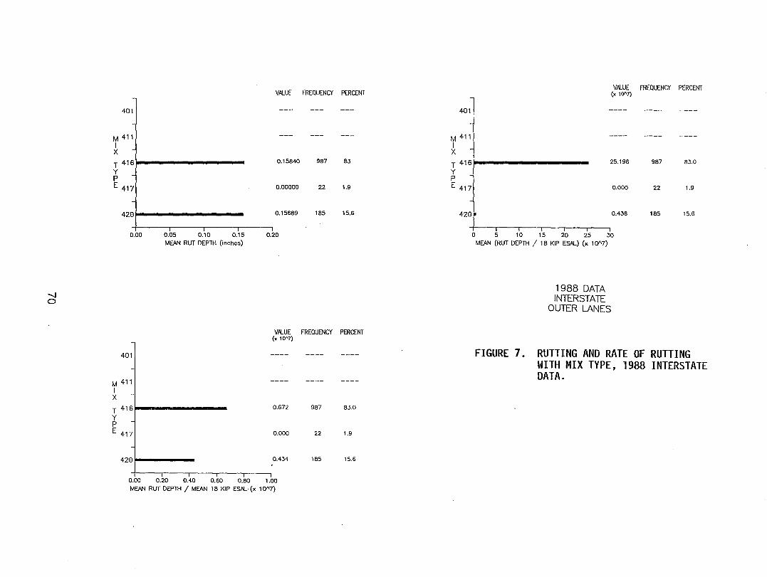
'-l o
VALUE
401
M 411 I X T 416 0.15840
Y p E 417 0.00000
420 0.15689
0.00 0.05 0.10 0.15 0.20 MEAN RUT DEPTH (inches)
VALUE (x 10'7)
4011
M 411' I X
T 4161 0.672
Y P E] 0.000
0.434
0.00 0.20 0.40 0.60 O.BO 1.00
MEAN RUT DEPTH / MEAN 1 B KIP ESAL· (x 10"7)
FREQUENCY PERCENT
987 83
22 1.9
185 15.6
FREQUENCY PERCENT
987 83.0
22 1.9
185 15.6
VALUE FREQUENCY PERCENT (x 10'7)
l 401
M 411 I X T 416' 25.196 987 83.0
Y P E 4171 0.000 22 1.9
42t-0.436 185 15.6
I I I I I I 0 5 10 15 20 25 30
MEAN (RUT DEPTH / 18 KIP ESAL) (x 10"7)
1988 DATA INTERSTATE
OUTER LANES
FIGURE 7. RUTTING AND RATE OF RUTTING WITH MIX TYPE, 1988 INTERSTATE DATA.
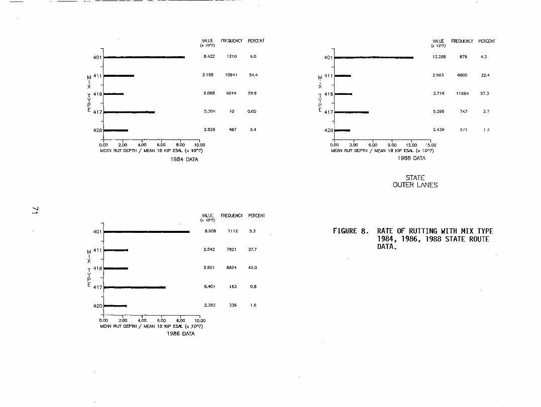
-....J ...L
V.AL.UE FREQUENCY PERCENT (x 10"7)
"1
4011~-------------------
"" M4111---1 X T416~ Y P E 417rl------
42011-0--
8.422
3.168
2.068
5.304
2.529
0.00 2.00 4.00 6.00 8.00 10.00 MEAN RUT DEPTH / MEAN 18 KIP ES/>L (x 10"7)
1984 DATA
V.AL.UE (x 10"7)
4011 8.908
M 4111 2.542
I X
T 416 1 2.501
Y P E] 6.401
2.385
I T---' 0.00 2.00 4.00 6.00 8.00 10.00 MEAN RUT DEPTH / MEAN 18 KIP ES/>L (x ,10"7)
1986 DATA
1210 6.0
10941 54.4
6014 29.9
10 0.05
487 2.4
FREQUENCY PERCENT
1112 5.3
7921 37.7
8824 42.0
163 0.8
336 .1.6
V.AL.UE FREQUENCY PERCENT (x 10"7)
12.288 876 4.3 40C M 411 2.503 6605 32.4
1 X
2.716
5.295
2.439
0.00 3.00 6.00 9.00 12.00 15.00 MEAN RUT DEPTH / MEAN 18 KIP ES/>L (x 10"7)
1988 DATA
STATE OUTER LANES
11664 57.3
747 3.7
271 1.3
FIGURE 8. RATE OF RUTTING WITH MIX TYPE 1984, 1986, 1988 STATE ROUTE DATA.
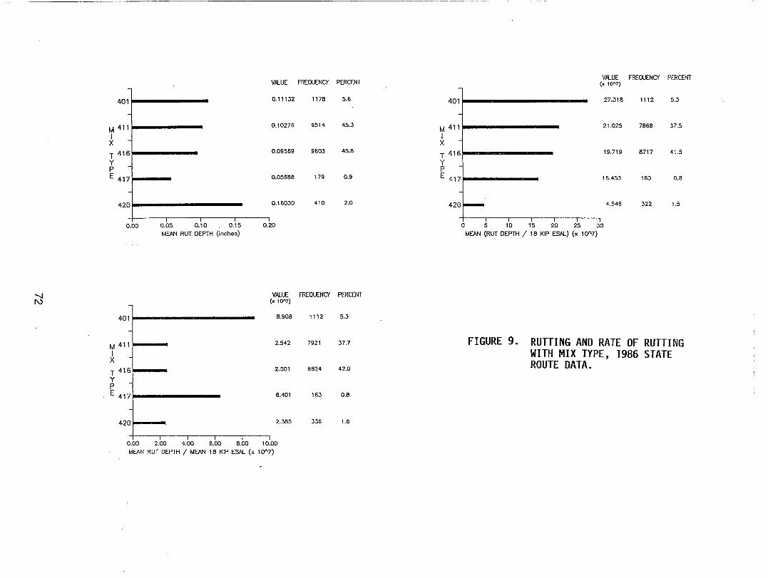
VAlUE FREQUENCY PERCENT VAlUE FREQUENCY PERCENT
(x 10"7)
4011
0.11132 1178 5.6 401 ' 27.318 1112 5.3
M 411 0.10276 9514 45.3 M 411' 21.025 7868 37.5
1 1 X X
T 416 0.09569 9603 45.8 T 416' 19.719 8717 41.5
Y Y P P E 417 0.05688 179 0.9 E 4171 16.453 163 0.8
420 0.16030 410 2.0 42t=
4.546 322 1.5
---, 0.00 0.05 0.10 0.15 0.20 0 5 10 15 20 25 30
MEAN RUT DEPTH (inches) MEAN (RUT DEPTH / 18 KIP ESAL) (x 1 Ql\7)
-.....J VAlUE FREQUENCY PERCENT I\) (x 10"7)
401 8.908 1112 5.3
M 411 2.542 7921 37.7 FIGURE 9. RUTTING AND RATE OF RUTTING 1 WITH MIX TYPE, 1986 STATE X
T 416 2.501 8824 42.0 ROUTE DATA. y p E] 6.401 163 0.8
2.385 336 1.6
, , , , 0.00 2.00 4.00 6.00 8.00 10.00
MEAN RUT DEPTH / MEAN 18 KIP ESAL (x 1Q1\7)
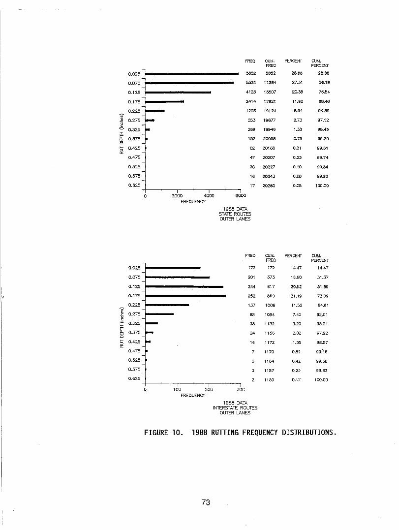
FREQ CUM. PERCENT CUM. FREQ PERCENT
-0.025 5852 5852 28.68 28.88
-0.075 5532 11384 27.31 56.19
-0.125 4123 15507 20.35 76.54
-0.175 2414 17921 11.92 88.46
-0.225 1203 19124 5.94 94.39
UJ -II)
0.275 - 553 19677 2.73 97.12 ..c 0 c:: -= 0.325 - 269 19946 1.33 98.45 ~ -a.. 0.375 • 152 20098 0.75 99.20 UJ 0 -~ 0.425 62 20160 0.31 99.51 0::: -
0.475 47 20207 0.23 99.74 -
0.525 20 20227 0.10 99.84 -
0.575 16 20243 0.08 99.92 -
0.625 17 20260 0.08 100.00 I I
0 2000 4000 6000
FREQUENCY
1988 DATA STATE RaLITES OUTER LANES
FREQ CUM. PERCENT CUM. FRED PERCENT -
0.025 172 172 14.47 14.47 -
0.075 201 373 16.90 31.37 -
0.125 244 617 20.52 51.89 -
0.175 252 869 21.19 73.09 -
0.225 137 1006 11.52 84.61 "OJ' -
Q) 0.275 88 1094 7.40 92.01 ..c
0 c:: -= 0.325 ~ 38 1132 3.20 95.21 ~ -a.. 0.375 ~ 24 1156 2.02 97.22 w 0 -f-- 0.425 ~ 16 1172 1.35 98.57 ::> 0::: -
0.475 • 7 1179 0.59 99:16 -0.525 5 1184 0.42 99.58
-0.575 3 1187 0.25 99.83 -0.625 2 1189 0.17 100.00
I I I 0 100 200 300
FREQUENCY
1988 DATA INTERSTATE ROUTES
OLITER LANES
FIGURE 10. 1988 RUTTING FREQUENCY DISTRIBUTIONS.
73
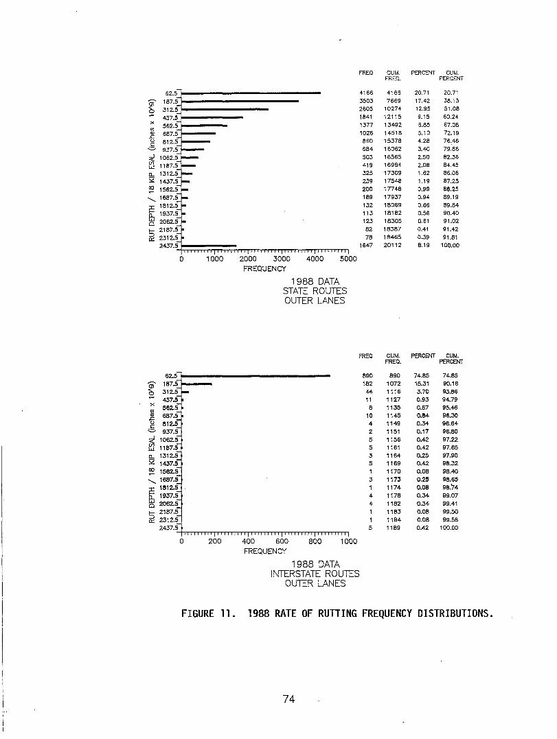
FREQ CUM. PERCENT CUM. FREQ. PERCENT
62.5 4166 4166 20.71 20.71 ,-.. 187.5 3503 7669 17.42 38.13
~ 312.5 2605 10274 12.95 51.08
437.5 1841 12115 9.15 60.24 x
562.5 1377 13492 6.85 67.08 III <ll 687.5 1026 14518 5.10 72.19 .c u 812.5 860 15378 4.28 76.46 c = 937.5 684 16062 3.40 79.86
<i! 1062.5 503 16565 2.50 82.36 (fJ 1187.5 419 16984 2.08 84.45 W
a.. 1312.5 325 17309 1.62 86.06 s:: 1437.5 239 17548 1.19 87.25 CO 1562.5 200 17748 0.99 88.25
-....... 1687.5 189 17937 0.94 89.19
F 1812.5 132 18069 0.66 89.84
a.. 1937.5 113 18182 0.56 90.40 W 2062.5 123 18305 0.61 91.02 0 I- 2187.5 82 18387 0.41 91.42 :::J 2312.5 78 18465 0.39 91.81 0::
2437.5 1647 20112 8.19 100.00
0 1000 2000 3000 4000 5000 FREQUENCY
1988 DATA STATE ROUTES OUTER LANES
FREQ CUM. PERCENT CUM. FREQ. PERCENT
62.5 890 890 74.85 74.85
g 187.5 182 1072 15.31 90.16 312.5 44 1116 3.70 93.86
437.5 11 1127 0.93 94.79 x
562.5 8 III
1135 0.67 95.46 <ll 687.5 10 1145 0.84 96.30 .c 0 812.5 4 1149 0.34 96.64 c = 937.5 2 1151 0.17 96.80
~ 1062.5 5 1156 0.42 97.22
w 1187.5 5 1161 0.42 97.65
a.. 1312.5 3 1164 0.25 97.90 s:: 1437.5 5 1169 0.42 98.32 CO 1562.5 1 1170 0.08 98.40
-....... 1687.5 3 1173 0.25 98.65
F 1812.5 1174 0.08 98.74
a.. 1937.5 4 1178 0.34 99.07 w 2062.5 4 1182 0.34 99.41 0 I- 2187.5 1183 0.08 99.50 :::J 2312.5 1184 0.08 99.58 0::
2437.5 5 1189 0.42 100.00
0 200 400 600 800 1000 FREQUENCY
1988 DATA INTERSTATE ROUTES
OUTER LANES
FIGURE 11. 1988 RATE OF RUTTING FREQUENCY DISTRIBUTIONS.
74
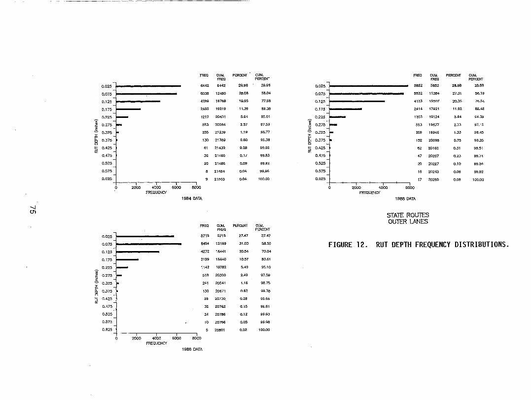
mEQ CUM. PERCENI" CUM. FREQ CUM. PERCENI" CUM. FREQ PERCENI" mEQ PERCENI"
-0.025 6442 6442 29.96 29.96 0.025 5852 5852 2B.88 28.88
-0.075 6038 12480 28.08 58.04 0.075 5532 11384 27.31 56.19
-0.125 4289 16769 19.95 77.98 0.125 4123 15507 20.35 76.54
-0.175 2450 19219 11.39 89.38 0.175 2414 17921 11.92 88.46
-~ 0.225 1212 20431 5.64 95.01 0.225 1203 19124 5.94 94.39
-;;;- - ~ ~ 0.275 ~ 553 20984 2.57 97.59 .c: 0.275 553 19677 2.73 97.12 g - u c:
<=0 0.325 I- 255 21239 1.19 98.77 <=0 0.325 269 19946 1.33 98.45 i!: ~ Ih 0.375 130 21369 0.60 99.38 0.375 152 20098 0.75 99.20 0 - 0
5 0.425 61 21430. 0.28 99.66 ~ 0.425 62 20160 0.31 99.51 a::
0.475 36 21466 0.17 99.83 0.475 47 20207 0.23 99.74 -
0.525 20 21486 0.09 99.92 0.525 20 20227 0.10 99.84 -0.575 8 21494 0.04 99.96 0.575 16 20243 0.08 99.92
0.625 21503 0.04 100.00 0.625 17 20260 0.08 100.00 I I I
0 2000 4000 6000 BODO 0 2000 4000 6000 FREQUENCY FREQUENCY
19B4 DATA 1988 DATA
-..J (J1
SfAIT ROU1ES OU1ER LANES
FREQ CUM. PERCENI" CUM. mEQ PERCENI"
0.025 5715 5715 27.47 27.47
0.075 6454 12169 31.03 58.50 FIGURE 12. RUT DEPTH FREQUENCY DISTRIBUTIONS. 0.125 4272 16441 20.54 79.04
0.175 2199 18640 10.57 89.61
0.225 - 1142 19782 5.49 95.10 -;;;-" 0.275 - 518 20300 2.49 97.59 .c: u c:
<=0 0.325 • 241 20541 1.16 98.75
~ 0.375 130 20671 0.62 99.38 0
5 0.425 59 20730 0.28 99,66 a::
0.475 32 20762 0.15 99.81
0.525 24 20786 0.12 99.93
0.575 10 20796 0.05 99.98
0.625 5 20801 0.02 100.00
0 2000 4000 6000 BODO FREQUENCY
1986 DATA
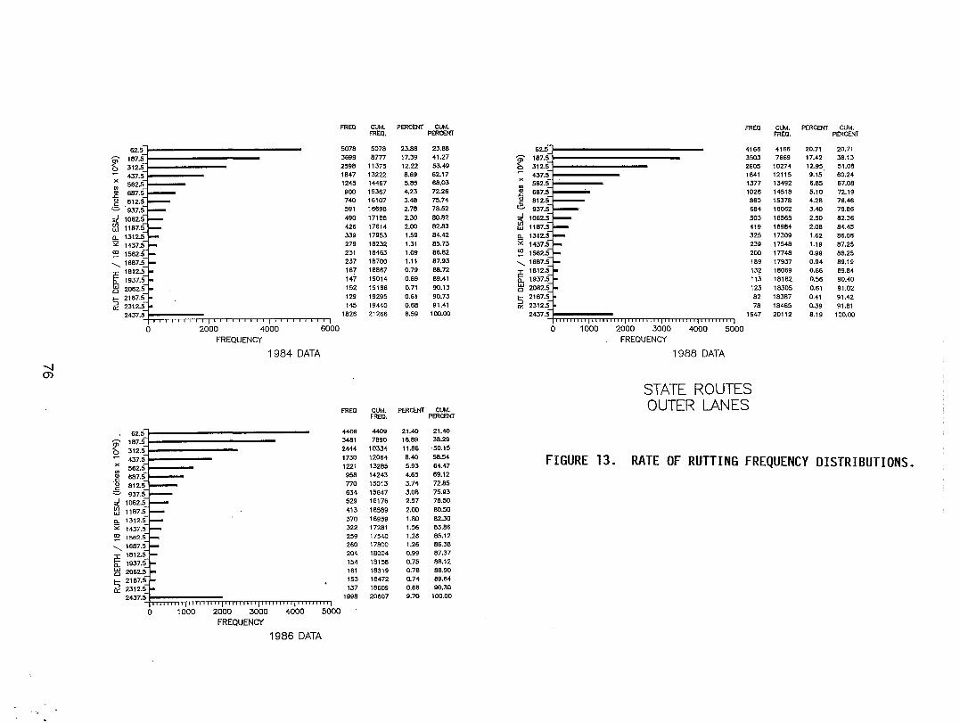
--..J (J)
62.5
R Q;' 187.51-----------b 312.5!-. -------
437.5] : 562.5l~----~ 687.S g 812.S = 937.S
~ 1062.~ w 1187.5 a.. 1312.S 52 1437.S CO 1562.S
........ 1687.S
F 1812.~ a.. 1937.5 gJ 2062.S
'3 2187.~ OC 2312.5
2437.S4q:;::;:~~:;::;,I".."..rr-r-.r~..,....,..~~ o 2000 4000
FREQUENCY
1984 DATA
~ ~;!~1t:::::::::::::::::::::::----437.~I-' ------x
III 562.~ ~ 687.5 g 812.S
c.. 937.5 <f. 1062.5 Ul -w 1187.5 a.. 1312.5 52 1437.S CO 1562.S
........ 1687.5
F 1812.5
~ '3 oc
o 1000 2000 3000 FREQUENCY
4000
6000
5000
1986 DATA
FREa CUM. PERCENT CUM. FREa. PERCENT
5078 5078 23.88 23.88 3699 8777 17.39 41.27 2598 11375 12.22 53.49 1847 13222 8.69 62.17 1245 14467 5.85 68.03 900 15367 4.23 72.26 740 16107 3.48 75.74 591 16698 2.78 78.52
490 17188 2.30 80.82 426 17614 2.00 82.83 339 17953 1.59 84.42 279 18232 1.31 85.73
231 18463 1.09 86.82 237 18700 1.11 87.93 167 18867 0.79 88.72 147 19014 0.69 89.41 152 19166 0.71 90.13 129 19295 0.61 90.73 145 19440 0.68 91.41
1826 21266 8.59 100.00
FREa CUM. PERCENT CUM. FREa. PERCENT
4409 3481
2444 1730 1221 958 770 634 529
413
4409 7890
10334 12064 13285 14243 15013 15647 16176
16589 370 16959 322 17281 259 17540 260 17800 204 18004 154 18158 161 18319 153 18472 137 18609
1998 20607
21.40 16.89 11.86 8.40 5.93 4.65 3.74 3.08 2.57
2.00
21.40 38.29 50.15 58.54 64.47 69.12 72.85 75.93 78.50 80.50
1.80 82.30 1.56 83.86 1.26 85.12 1.26 86.38 0.99 87.37 0.75 88.12 0.78 88.90 0.74 89.64 0.66 90.30 9.70 100.00
62.5 11----------------,..... 187.5
~ 312.sll---------437.S~
III 562.5 -----~ 687.5 p', ---'
812.5 ~ 937.5
~ 1062.~ w 1187.5 a.. 1312.5
1437.5 52
~ 1562.5 ........ 1687.5
F 1812.~ a.. 1937.5 gJ 2062.5
'3 2187.~ oc 2312.5
24J7.sl, iii i I Iii Iii iii Iii iii iii Iii i I I , ] iii iii Iii iii iii iii
o 1000 2000 3000 FREQUENCY
4000 5000
1988 DATA
FREa CUM. PERCENT CUM. FREa. PERCENT
4166 4166 20.71 20.71 3503 7669 17.42 38.13 2605 10274 12.95 51.08 1841 12115 9.15' 60.24 1377 13492 6.85 67.08 1026 14518 5.10 72.19 860 15378 4.28 76.46 684 16062 3.40 79.86
503 16565 2.50 82.36 419 16984 2.08 84.45 325 17309 1.62 86.06 239 17548 1.19 87.25 200 17748 0.99 88.25 189 17937 0.94 89.19 132 18069 0.66 89.84 113 18182 0.56 90.40 123 18305 0.61 91.02 82 18387 0.41 91.42 78 18465 0.39 91.81
1647 20112 8.19 100.00
STATE ROUTES OUTER LANES
FIGURE 13. RATE OF RUTTING FREQUENCY DISTRIBUTIONS.
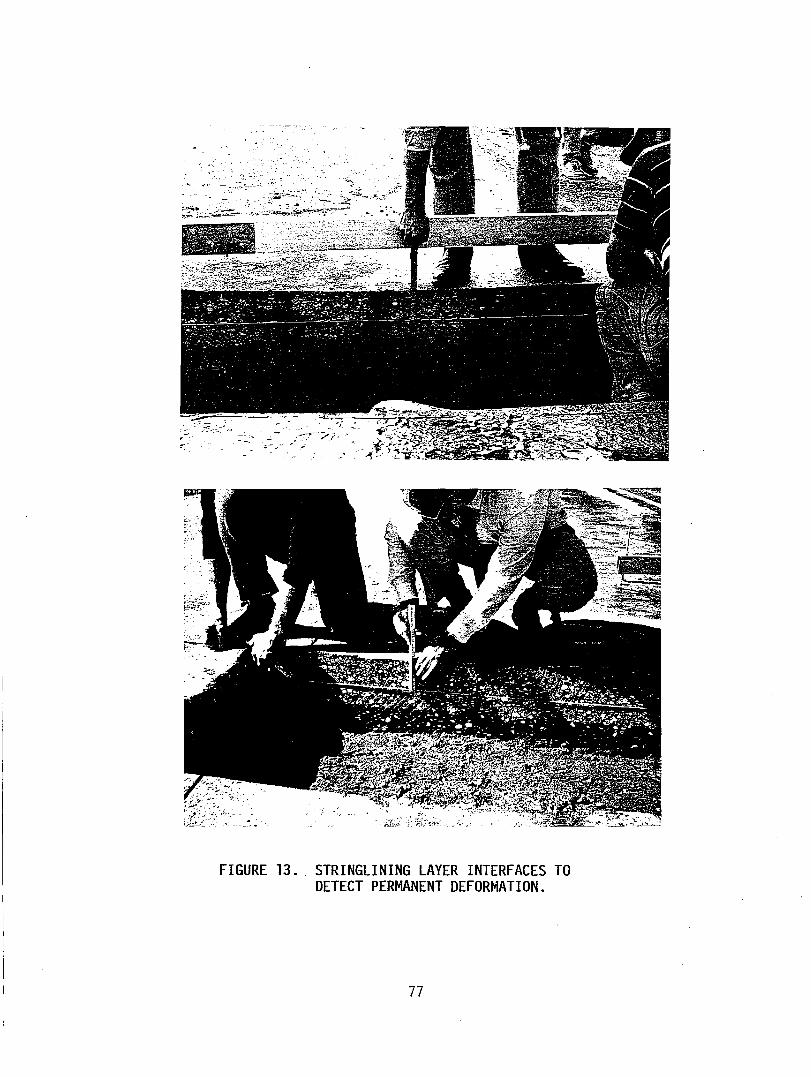
.-.-:-~~,.;;,::.~=-:~ .... -~. ',-... ::. .. ~~:"). ~~- 3='~"·
~.t:~~j;~-":·~,~~::~:".;,;,i:,o~';;;;~
FIGURE 13. STRINGLINING LAYER INTERFACES TO DETECT PERMANENT DEFORMATION.
77
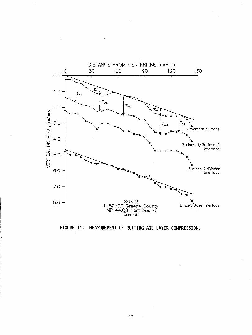
en (l) ..c u c
W u z ~ (f)
0
<e u l-n:::: w >
0 0.0
1.0 T •.
2.0
3.0
4.0
5.0
6.0
7.0
8.0
DISTANCE FROM CENTERLINE, inches 30 60 90
Site 2 1-59/20 Greene County
MP 44.00 Northbound Trench
120 150
Pavement Surface
Surface 1/Surface 2 Interface
Surface 2/Binder Interface
Binder/Base Interface
FIGURE 14. MEASUREMENT OF RUTTING AND LAYER COMPRESSION.
78
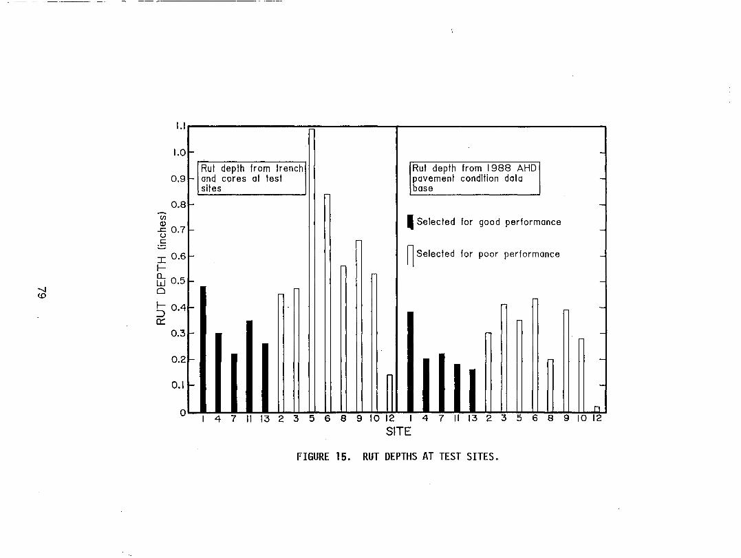
-...j CD
1.1_. ----n---,------i 1.01-
........ !J) Q)
Rul deplh from Irench 0.91-1 and cores 01 lesl
sites
0.81-
.J:: 0.71-u c:
I 0.61-f-0.... W 0.51-o I-:::> 0041-c::
0.31-
0.21-
0.11-
Rut depth from 1988 AHD pavement condition data base
,Selected for good performance
n Selected for poor performance
-
--
-
-
-
-
-
-
-
0' • • • • • !! !! I! I! II II II II' ••••• II II II II II II !! 0 , 1 4 7 II 13 2 3 5 6 8 9 10 12 I 4 7 1\ 13 2 3 5 6 8 9 10 12
SITE
FIGURE 15. RUT DEPTHS AT TEST SITES.
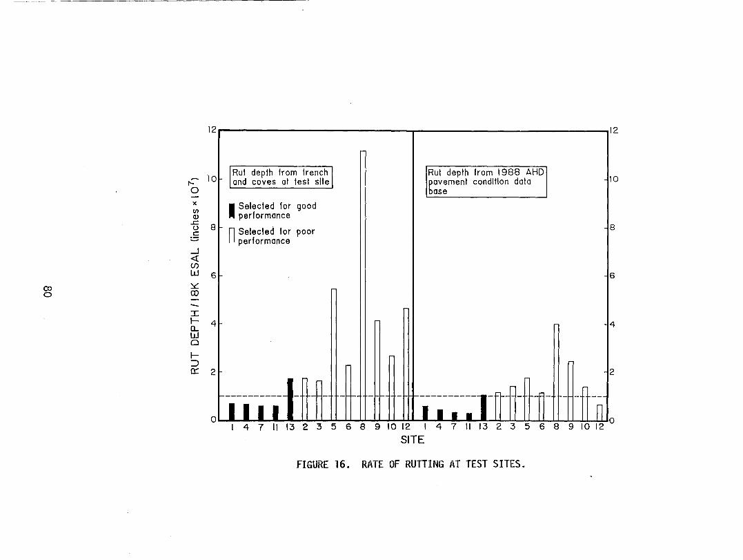
12 12
10 I'-0
I Rut depth from trench Rut depth from 1988 AHD ,
and coves at test site bavement conditlon data ase
o
x III Q)
.c 8 u
c -
I Selected for good performance
n Selected for poor performance
8
--I « (J) w 6 I 6 ::L ro CO
0 -:r: I- 4 Il... 4 W 0
I-::J 0::: 2 2 ,
------------ - - - - I--~ - 1--. - 1------------1- .- - ,..- - - - --II_I J I • I _I n o I 4 7 II 13 2 3 5 6 8 9 10 12 I 4 7 II 13 2 3 5 6 8 9 10 12 0
SITE
FIGURE 16. RATE OF RUTTING AT TEST SITES.
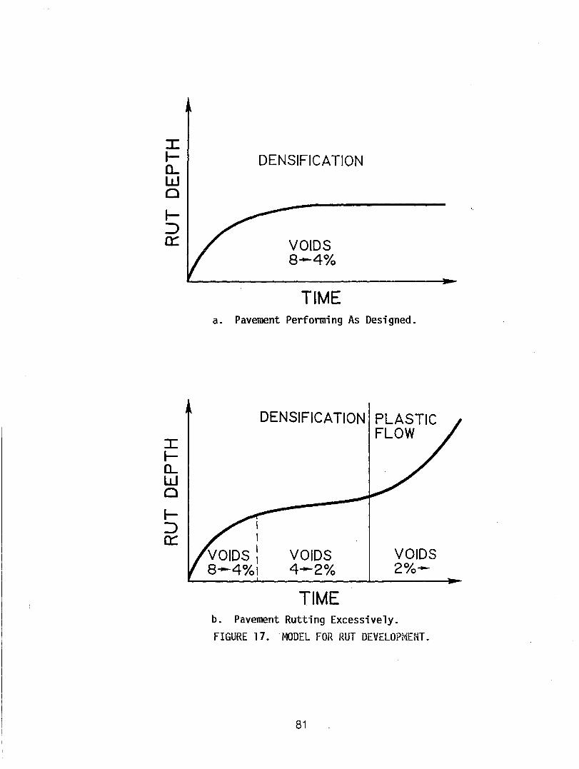
:c Ia.. W o I:::> 0:::
DENSIFICATION
VOIDS 8-4%
TIME a. Pavement Performing As Designed.
I I
VOIDS: 8-4%1
DENSIFICATION PLASTIC FLOW
VOIDS 4-2%
TIME
VOIDS 2%-
b. Pavement Rutting Excessively. FIGURE 17. . MODEL FOR RUT DEVELOPj4ENT.
81
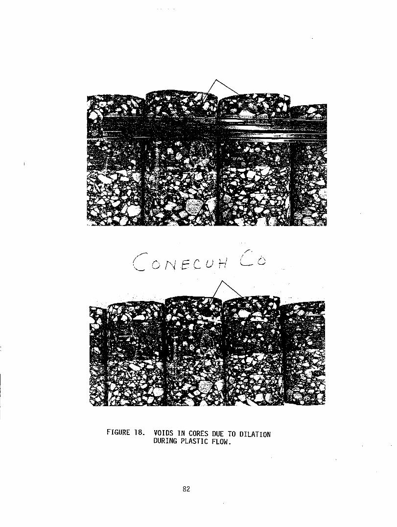
FIGURE 18. VOIDS IN CORES DUE TO DILATION DURING PLASTIC FLOW.
82
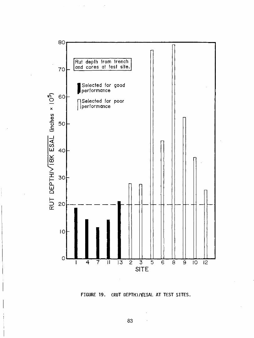
80
70 I-Rut depth from trench and cores at test site.
-J Selected for good
performance 10 60 0
x
l- n Selected for poor performance
U) Q) ~
50 (.) I-c:
.....J « CJ) w 40 -~ 00
-I 30 I- -a... w a I-::J 20 _0 ______
1-- - - ..-- - - 1-- - -0:::
10 -
o 4 7 II 13 2 3 5 6 8 9 10 12
SITE
FIGURE 19. (RUT DEPTH)/f[SAL AT TEST SITES.
83
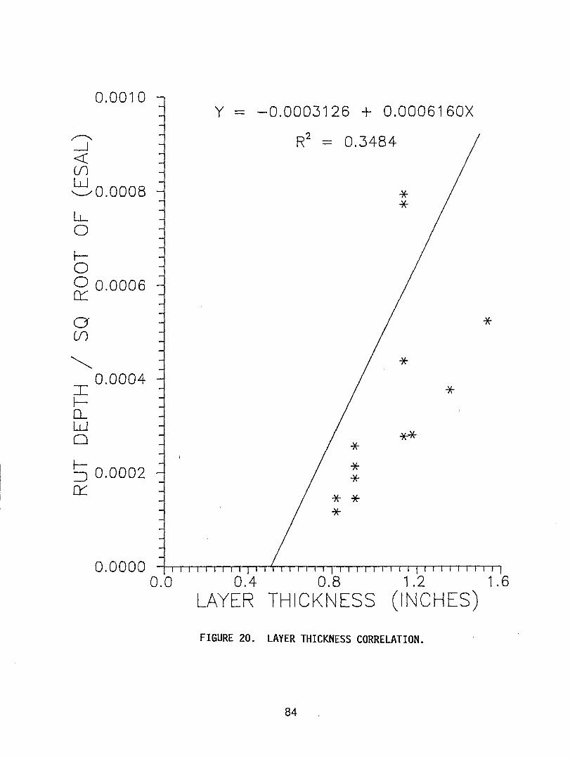
0.0010 Y - -0.0003126 + 0.0006160X
,--.. R2 == 0.3484 --.J <{ (f) w '--" 0.0008 * * LL 0
t-o ~ 0.0006
a * (f)
~ * 0.0004 ::r * ~
Il W 0 ** * t- * :J 0.0002
* 0::::: * * *
0.0000 0.0 0.4 0.8 1.2 1.6
LAYER THICKNESS (INCHES)
FIGURE 20. LAYER THICKNESS CORRELATION.
84
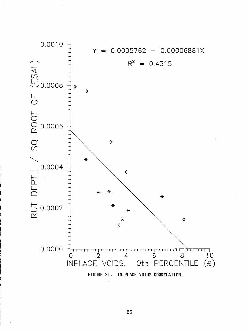
0.0010
,.,--.... .--J <C (f) w ,--,,0.0008
LL 0
r-0 ~ 0.0006
a (f)
~ 0.0004
:::r:: r-0.-w 0
r-::J 0.0002 n:::
0.0000
* *
Y - 0.0005762 - 0.00006881 X
R2 = 0.4315
*
* * * * *
* * *
02· 4 6 8 10 INPLACE VOIDS, Oth PERCENTILE (%)
FIGURE 21. IN-PLACE VOIDS CORRELATION.
85 .
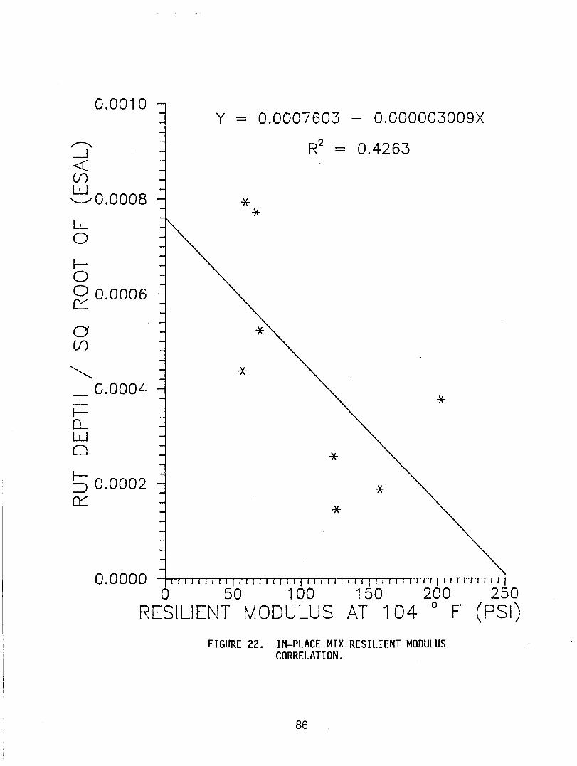
0,0010
,,--..... -' « (f)
~0,0008 LL o Io ~ 0.0006
a (f)
~ 0,0004
I l-n... w o
~ 0,0002 n::
Y - 0.0007603 - 0.000003009X
R2 = 0.4263
* *
* *
o 50 1 00 1 50 200 250 RESILIENT MODULUS AT 1 04 0 F (PSI)
FIGURE 22. IN-PLACE MIX RESILIENT MODULUS CORRELATION.
86 .
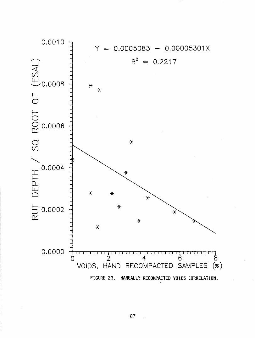
0.0010
,...--.... -1 <t (f) w ~0.OO08
LL 0
~ 0 ~ 0.0006
a U1
" 0.0004 I ~ CL W 0
t-:::) 0.0002 cr:
0.0000
Y - 0.0005083 - 0.00005301 X
R2 = 0.2217
* *
*
* * *
* *
02468 VOIDS, HAND RECOMPACTED SAMPLES (%)
FIGURE 23. MANUALLY RECOMPACTED VOIDS CORRELATION.
87
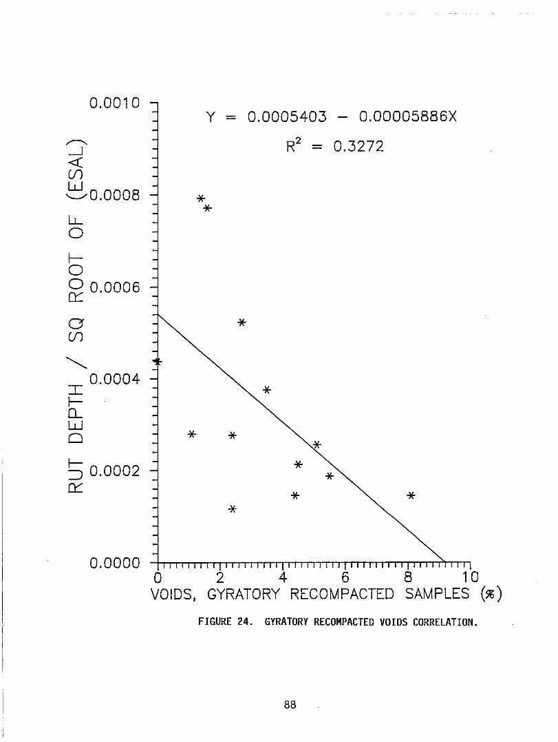
0.0010 Y - 0.0005403 - 0.00005886X
r-... R2 = 0.3272 -l « (f) w ,-",0.0008 * * LL 0
I-0 ~ 0.0006
a * (f)
~ 0.0004
I I-CL W 0 * * I-:J 0.0002 * cr:::
* * *
o 2 4 6 8 10 VOIDS, GYRATORY RECOMPACTED SAMPLES (%)
FIGURE 24. GYRATORY RECOMPACTED VOIDS CORRELATION.
88
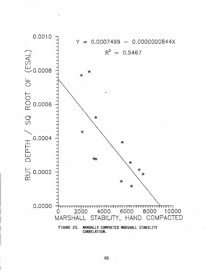
0.0010
,--..... --.J « (J) w ",-,,0.0008
Lt-0
r-0 ~ 0.0006
a (J)
~
I 0.0004
r-0.. w 0
r-:J 0.0002 0:::
0.0000
Y - 0.0007499 - 0.0000000844X
R2 = 0.5467
* *
* *
* * * *
o 2000 4000 6000 8000 1 0000 MARSHALL STABILITY, HAND COMPACTED
FIGURE 25. MANUALLY COMPACTED MARSHALL STABILITY CORRELATION.
·89
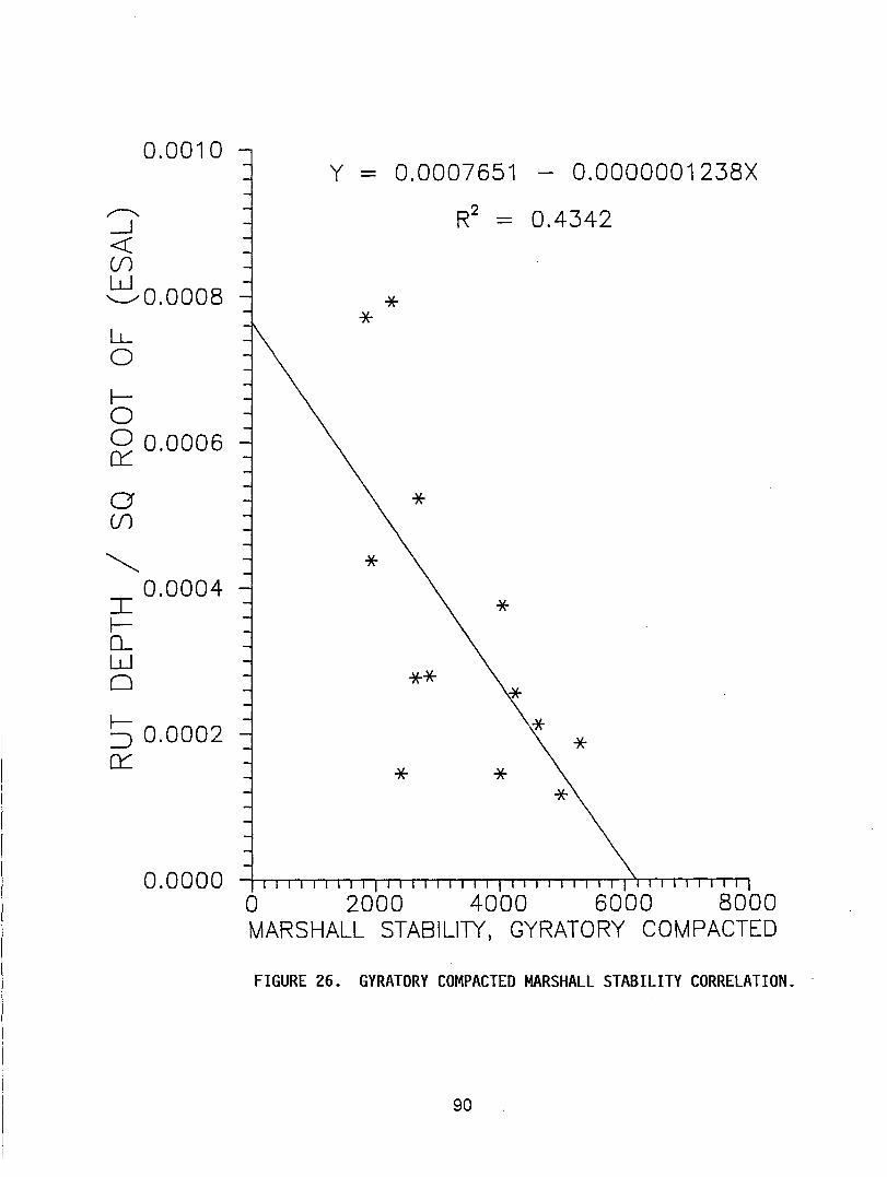
0.0010
r-... --1 <C if) w ,,--,0.0008
LL 0
r-0 ~ 0.0006
a if)
~ 0.0004
I r-CL W 0
r-:J 0.0002 0:::
0.0000
Y 0.0007651 - 0.0000001 238X
R2 = 0.4342
* *
* *
o 2000 4000 6000 8000 MARSHALL STABILITY, GYRATORY COMPACTED
FIGURE 26. GYRATORY COMPACTED MARSHALL STABILITY CORRELATION.
90
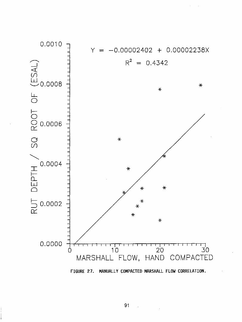
0.0010
~
-.J « (f) w ,-",0.0008
LL 0
I-0 ~ 0.0006
a (f)
~ 0.0004
I l-n... w 0
I-~ 0.0002 0:::
0.0000
Y - -0.00002402 + 0.00002238X
R2 = 0.4342
*
*
*
*
* *
* * *
*
o 10 20 30 MARSHALL FLOW, HAND COMPACTED
FIGURE 27. MANUALLY COMPACTED MARSHALL FLOW CORRELATION.
91
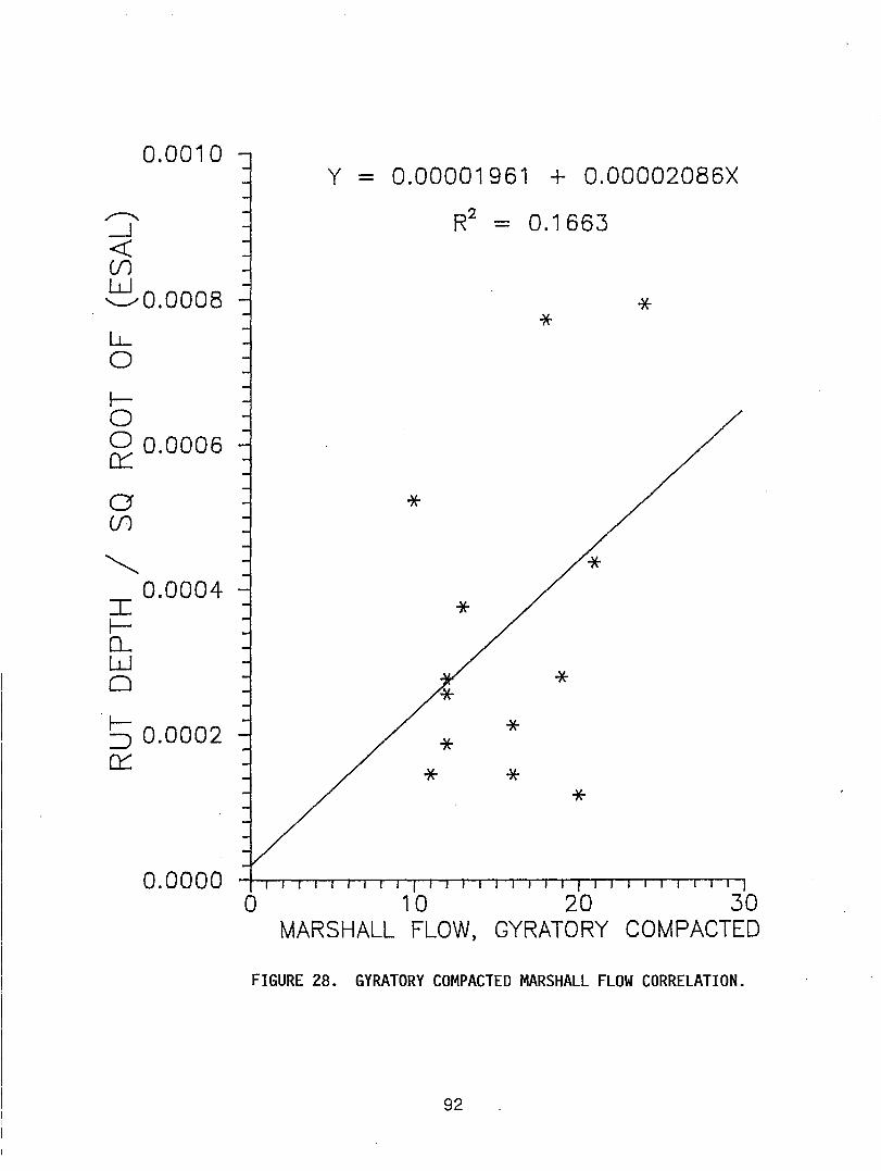
~
~ « (f)
0.0010
~0.0008 LL o I-o ~ 0.0006
a (J)
~ 0.0004
I l-n.. w o
.~ 0.0002 n:::
0.0000
Y - 0.00001961 + 0.00002086X
R2 = 0.1663
* *
*
*
* * *
* * *
o 10 20 30 MARSHALL FLOW, GYRATORY COMPACTED
FIGURE 28. GYRATORY COMPACTED MARSHALL FLOW CORRELATION.
92
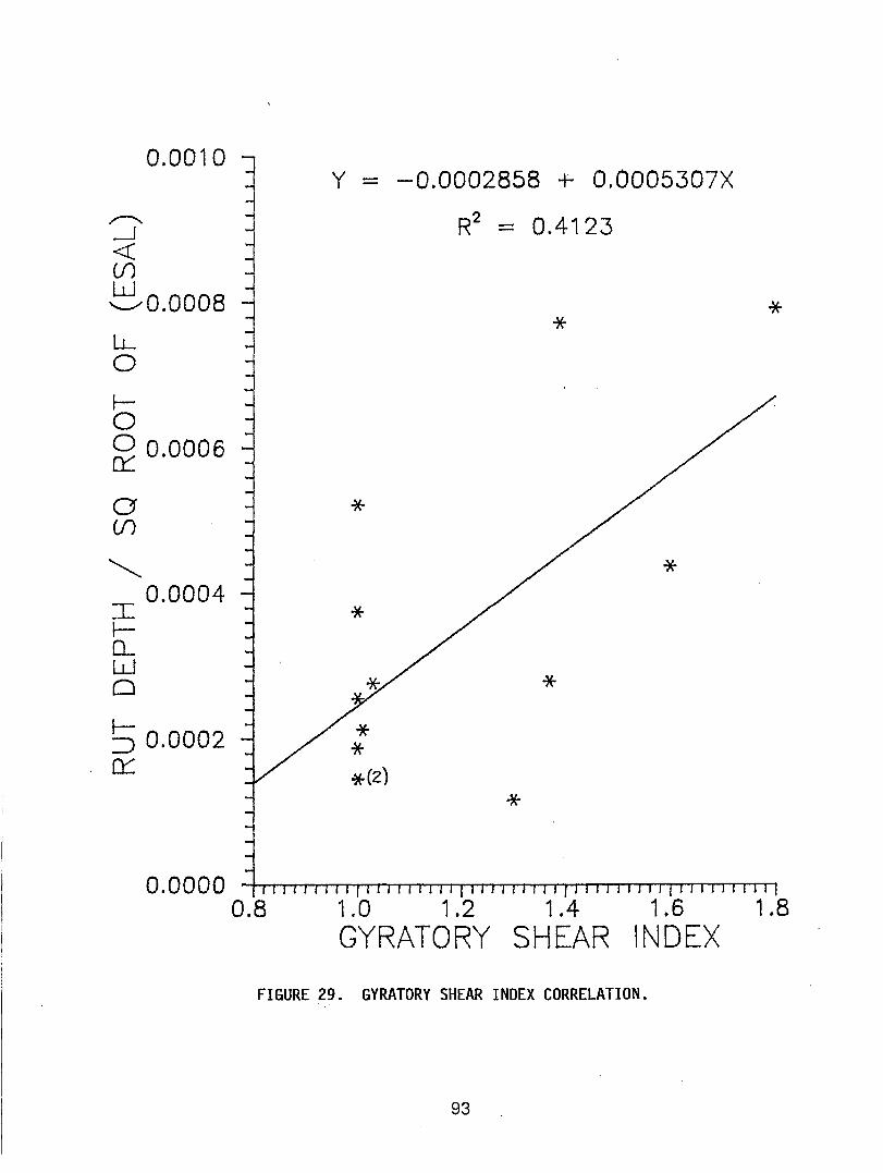
0.0010 Y - -0.0002858 + 0.OO05307X
",.-..... R2 = 0.4123 .-J <{ (/) w '--'" 0.0008 * * LL 0
~ 0 ~ 0.0006
a * (J)
~ * 0.0004
I * r-(L w 0 * t-:::J 0.0002 et:
*
o . 0 a 0 0 -h-r-r-r-Ir-r-r-r-r-T""'l"-r-r-r-.,-,-,-,..-,--.-,r-T""r'T..,....,..........,..,........'T'""r"T""~r-r-r-r-r-r-T......-r-r-r-T""T'""l
0.8 1.0 1.2 1.4 1.6 1.8 GYRATORY SHEAR INDEX
FIGURE 29. GYRATORY SHEAR INDEX CORRELATION.
93
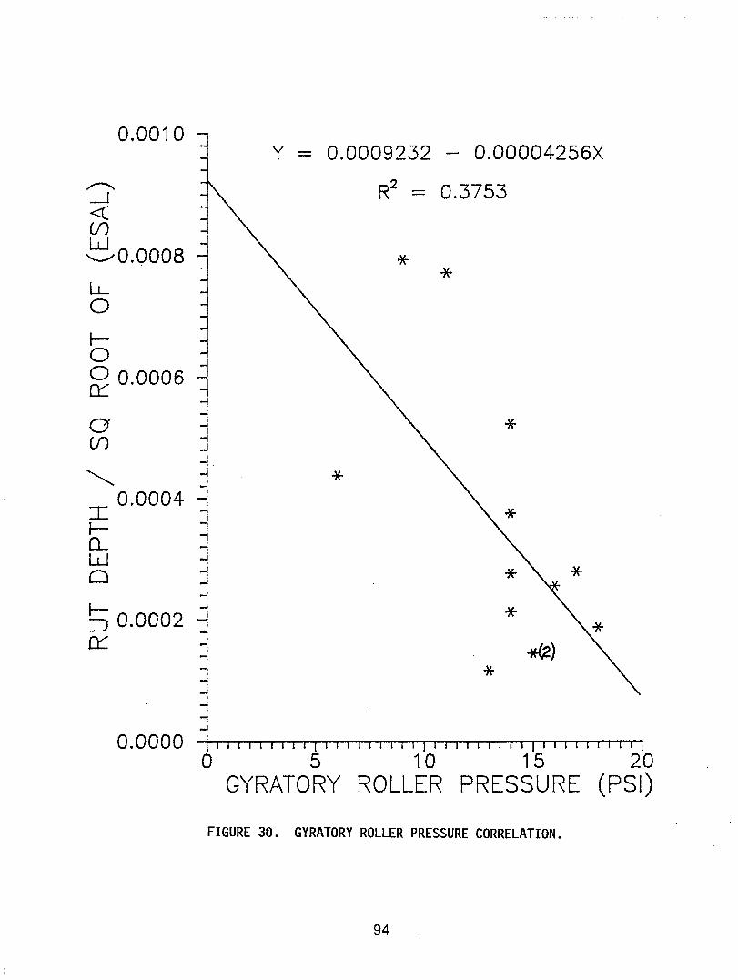
~
---l « en
0.0010
~O.0008 LL o I-o ~ 0.0006
a (f)
" 0.0004 I l-n... w o
~ 0.0002 n::
0.0000
Y - 0.0009232 - 0.00004256X
R2 = 0.3753
* *
*
*
o 5 10 15 20 GYRATORY ROLLER PRESSURE (PSI)
FIGURE 30. GYRATORY ROLLER PRESSURE CORRELATION.
94
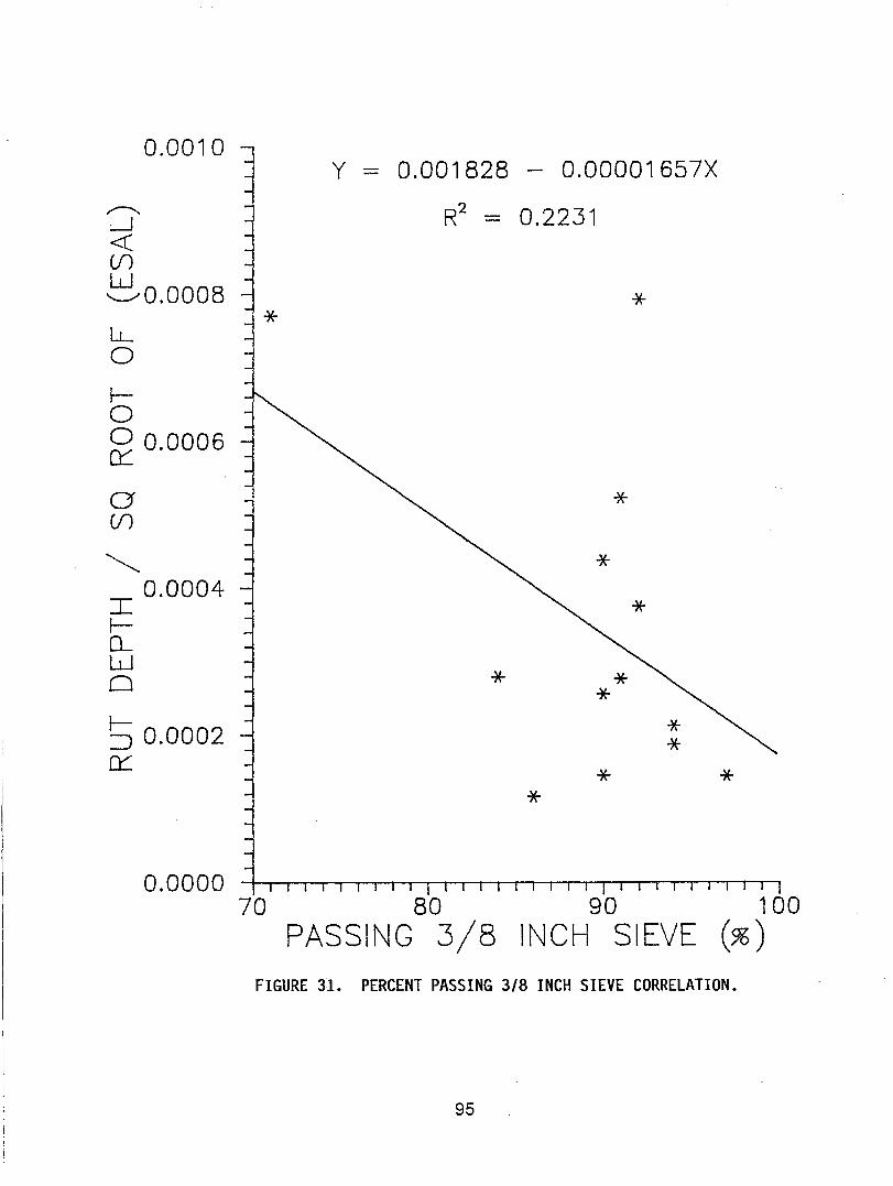
0.0010 Y - 0.001828 - 0.00001657X
,--... R2 = 0.2231 ~ <C if) w "--,,,0.0008 * * LL 0
I-0 ~ 0.0006
a * if)
~ * 0.0004
I * I-CL W 0 * * * I- * :J 0.0002 * n::::
* * *
0.0000 70 80 90 100
PASSING 3/8 INCH SIEVE (%) FIGURE 31. PERCENT PASSING 3/8 INCH SIEVE CORRELATION.
95
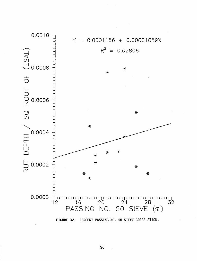
0.0010
r-.. -' « (f)
~0.0008 LL o Io ~ 0.0006
a (f)
~ 0.0004
I I--CL W o
~ 0.0002 a:::
0.0000
Y - 0.0001156 + 0.00001059X
R2 = 0.02806
*
12 16 20 24 28 32 PASSING NO. 50 SIEVE (%)
FIGURE 32. PERCENT PASSING NO. 50 SIEVE CORRELATION.
96
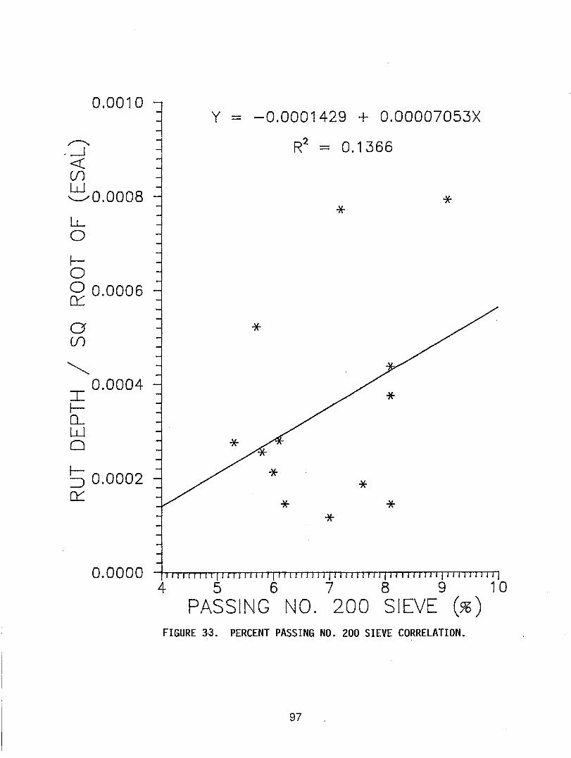
0.0010
r-.. - -.J « (f)
~0.0008 LL o tO ~ 0.0006
a (f)
~ 0.0004
I t-CL W o
~ 0.0002 0::::
Y -0.0001429 + 0.00007053X
R2 = 0.1366
* *
*
*
*
* * * *
0.0000 111111'1,1'111' J '1,11'11111/
4 5 6 7 8 9 10 PASSING NO. 200 SIEVE (%)
FIGURE 3,~. PERCENT PASSING NO. 200 SIEVE CORRELATION.
97
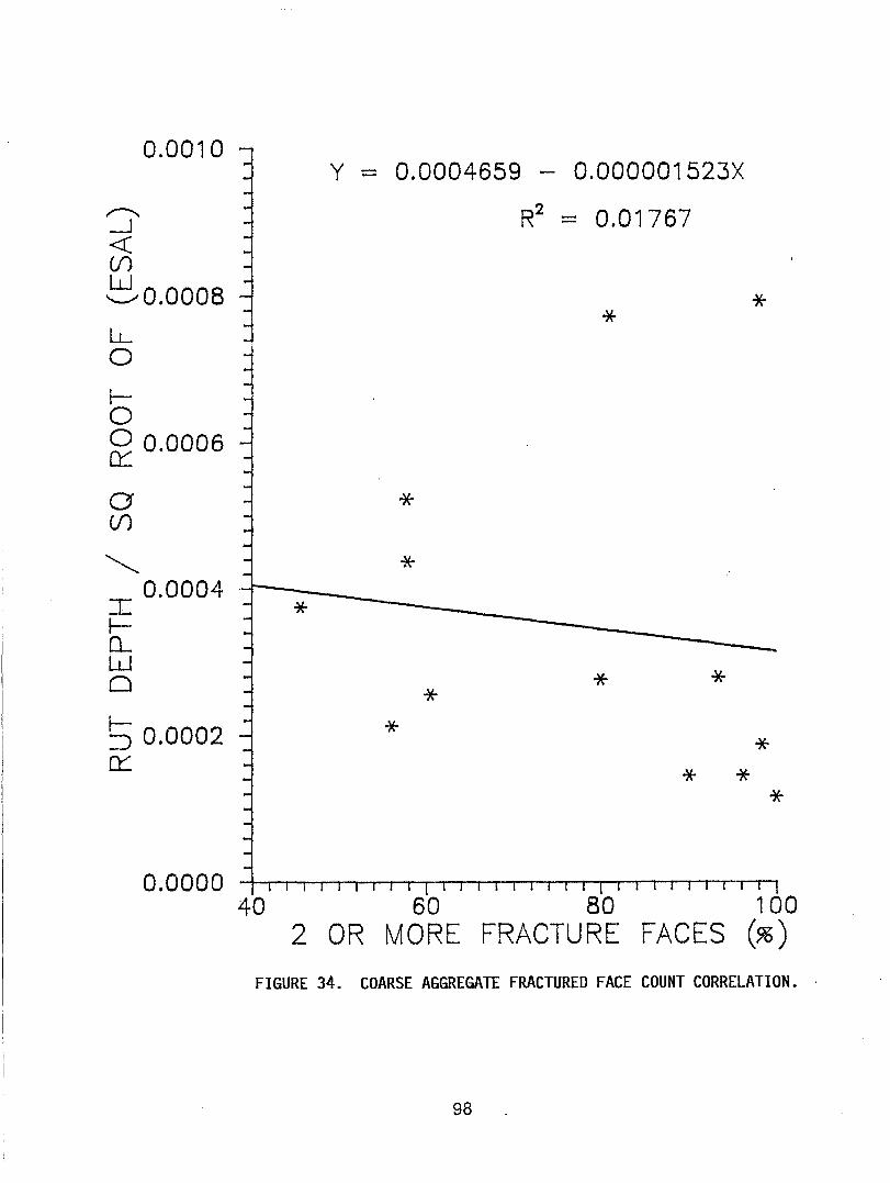
0.0010 Y - 0.0004659 - 0.000001523X
,--.... R2 = 0.01767 --.J <C if) w ~0.0008 * * LL 0
f-a ~ 0.0006
a * (f)
~ * 0.0004 I * t-o... W 0 * * * f- * :J 0.0002 * 0:::
* * *
0.0000 40 60 80 100
2 OR MORE FRACTURE FACFS (%) FIGURE 34. COARSE AGGREGATE FRACTURED FACE COUNT CORRELATION.
98
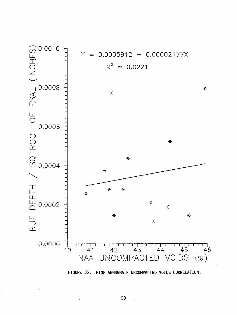
(/)0.0010 w I U Z
-.-1 0.0008 <{ (f) W
LL o ~ 0.0006 o o cr:: a (f) 0.0004
~
I ~ D-.. 2:S 0.0002
~.
:J cr::
Y - 0.0005912 + 0.00002177X
R2 = 0.0221
*
*
*
* * *
* * * * *
*
0.0000 I I I I I I I I I I I I I I I I I I I I I I I I I I 40 41 42 43 44 45 46
NAA UNCOMPACTED VOIDS (%) FIGURE 35. FINE AGGREGATE UNCOMPACTED VOIDS CORRELATION.
99
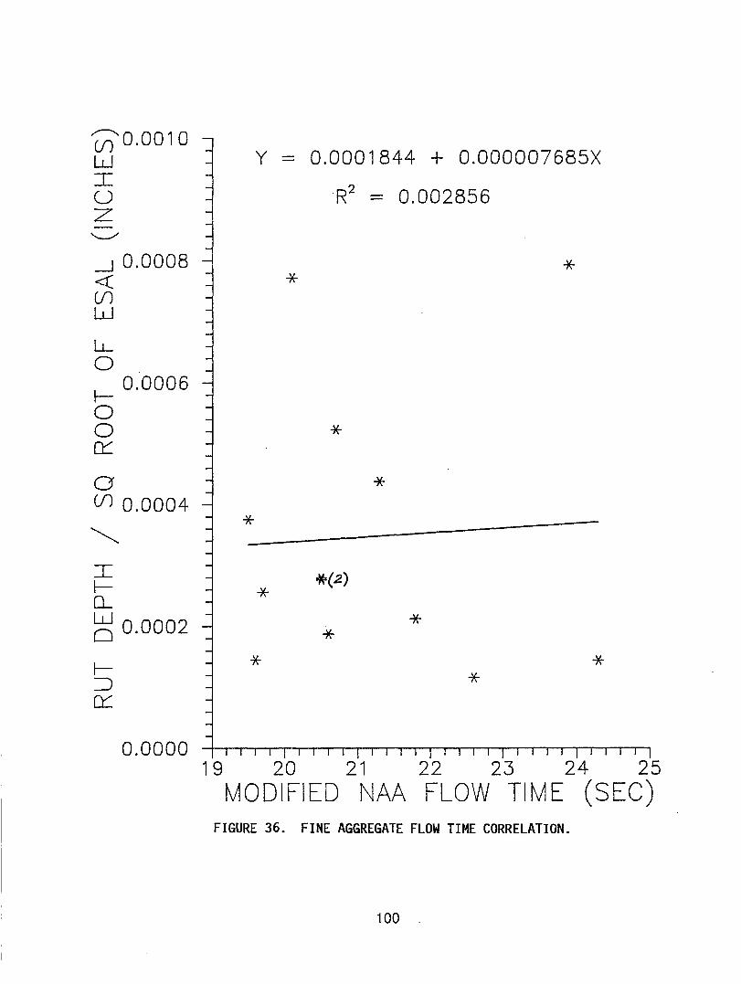
([)0.0010 w I U Z
--.J 0.0008 <t: (f) W
LL o I- 0.0006 o o 0:::
a (f) 0.0004
~
I I-0.-
~ 0.0002
I-=:J 0:::
*
Y - 0.0001844 + 0.000007685X
R2 = 0.002856
* *
*
*
* * *
* * *
0.0000 .1 1 I I I I 1 1 1 I j 1 1 I I I I 1 I I 1 1 1 1 I 19 20 21 22 23 24 25
MODIFIED NAA FLOW TIME (SEC) FIGURE 36. FINE AGGREGATE FLOW TIME CORRELATION.
100 .
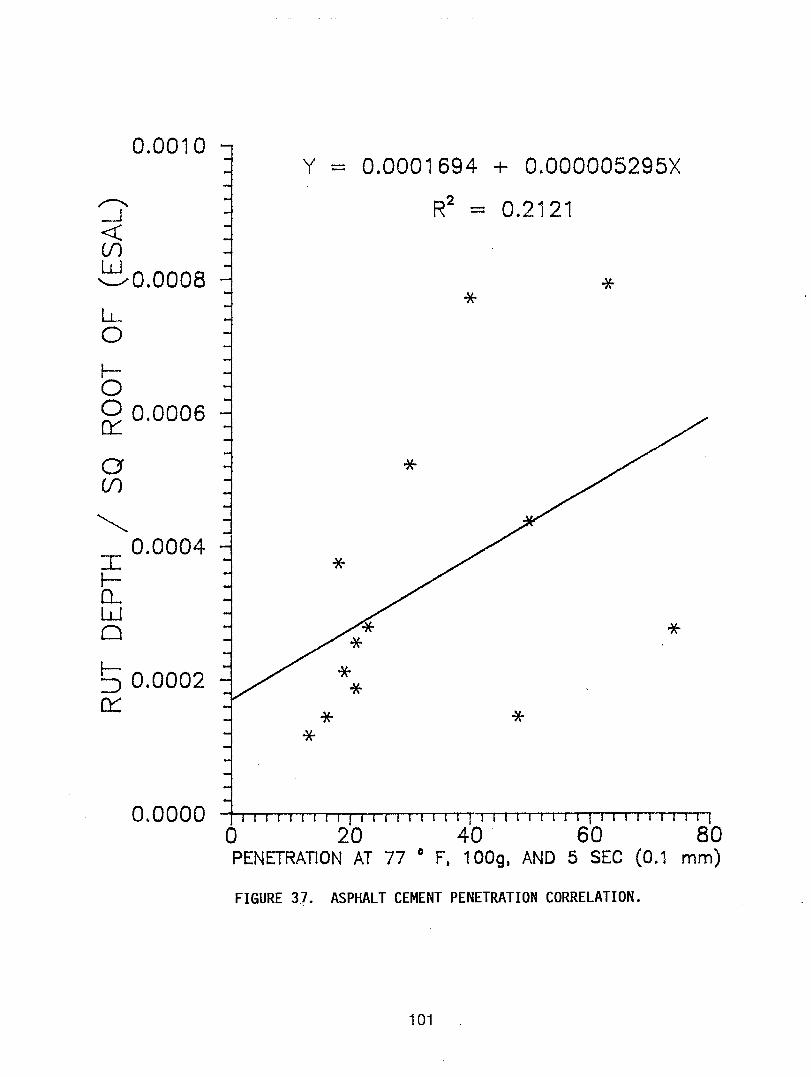
0.0010 Y - 0.0001694 + 0.000005295X
,,--..... R2 = 0.2121 -1 <{ if) w ~0.0008 * * I....L 0
~ 0 ~ 0.0006
a * if)
~ I 0.0004
* ~ 0... W 0 * r- * ::J 0.0002
* ~
* * *
0.0000 I I I I I I I I I I I I I I [ I I I I I o 20 40 60 80 PENETRATION AT 77 0 F. 1 DOg. AND 5 SEC (0.1 mm)
FIGURE 3.1. ASPHALT CEMENT PENETRATION CORRELATION.
101
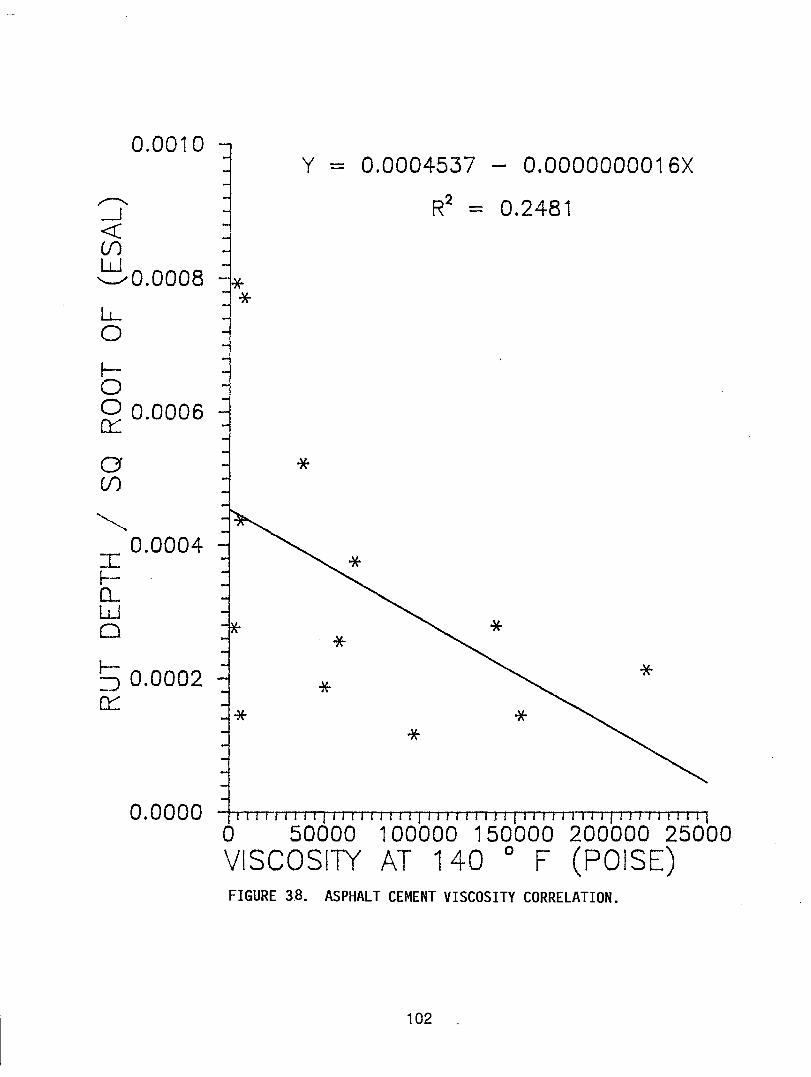
0.0010 Y - 0.0004537 - 0.00OOOOO016X
r-.. R2 = 0.2481 .--1 « (/) w . ,-,,0.0008
LL 0
f-0 ~ 0.0006
a * (J)
~
I 0.0004
r--(L w 0 * * f- * :J 0.0002
* c.t:: * *
0.0000 I I I I I I' I II I I I I I I'I I I I I I I I II I I I I I I I I II I T I I rTTTl o 50000 100000 150000 200000 25000 VISCOSITY AT 140 0 F (POISE) FIGURE 3.8. ASPHALT CEMENT VISCOSITY CORRELATION.
102 .
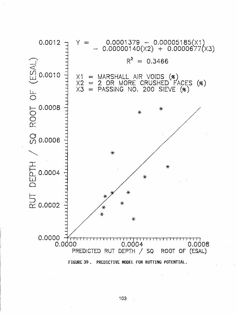
0.0012
,,--..... -' <C ~ 0.0010 '--"
LL 0
I- 0.0008 0 0 0:::
a (f) 0.0006
~
I r-CL 0.0004 w 0
r-:J cr:: 0.0002
y -
X1 -X2 -X3 -
0.0001379 - 0.00005185(X1) 0.00000140(X2) + O.0000677(X3)
R2 = 0.3466
MARSHALL AIR VOIDS (96) 2 OR MORE CRUSHED FACES ~) PASSING NO. 200 SIEVE (96)
*
*
* *
* *
0.0000 , r f I 1 I I I I I I 1111 J J I I ! I ! ) ! I I I 0.0000 0.0004 0.0008
PREDICTED RUT DEPTH / SQ ROOT OF (ESAL)
FIGURE 39 . PREDICTIVE MODEL FOR RUTTING POTENTIAL.
103 .
APPENDIX A
RUTTING DATA FROM PAVEMENT CONDITION DATABASES
104 .

DATA SORTED BY AHD DIVISION
105 .
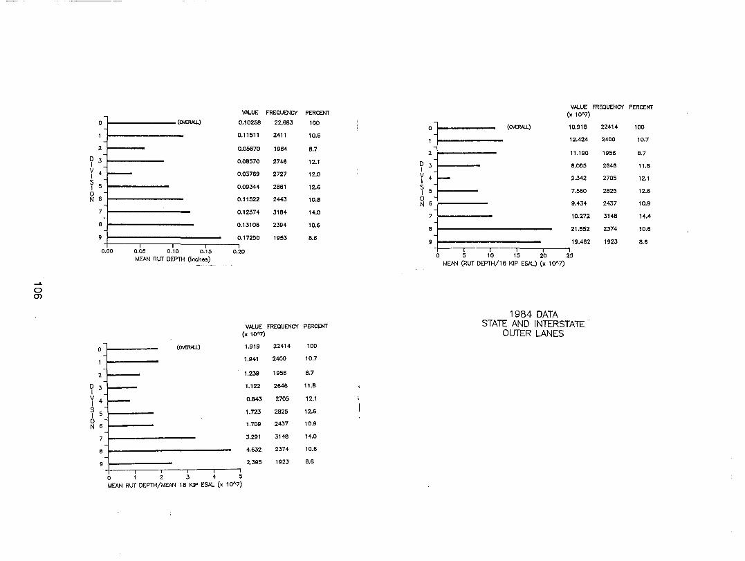
....... o (J)
o
2
o 3 I V 4 I S 5 I
2 6
7
8
9
~------------(~
~
0.00 0.05 0.10 0.15 MEAN RUT DEPTH (inch e.)
V,ALUE
0.10258
.11511
.05670
.08570
.03769
.09344
.11522
0.12574
0.13106
0.17250
0.20
FREQUE;NCY PERCENT
22,683 100
2411 10.6
1964 8.7
2746 12.1
2727 12.0
2861 12.6
2443 10.8
3184 14.0
2394 10.6
1953 8.6
V,ALUE FREQUENCY PERCENT
o
2
o 3 I V 4 I S 5 I
2 6
7
8
(0IIm'U)
-
o 1 2 3 4 5 MEAN RUT DEPTH/MEAN 18 KIP E5J'J... (x 10"7)
(x 10"7)
1.919
1.941
1.239
1.122
0.843
1.723
1.709
3.291
4.632
2.395
22414 100
2400 10.7
1956 8.7
2646 11.8
2705 12.1
2825 12.6
2437 10.9
3148 14.0
2374 10.6
1923 8.6
o
2
o 3 I V 4 I S 5 I
2 6
7
8
9
V,ALUE FREQUENCY PERCENT (x 10"7)
I--
0.918
2.424
1.190
8.085
2.342
7.560
9.434
10.272
21.552
19.462
o 5 10 15 20 25 MEAN (RUT DEPTH/18 KIP E5J'J...) (x 10"7)
1984 DATA STATE AND INTERSTATE
OUTER LANES
22414 100
2400 10.7
1956 8.7
2646 11.8
2705 12.1
2825 12.6
2437 10.9
3148 14.4
2374 10.6
1923 8.6
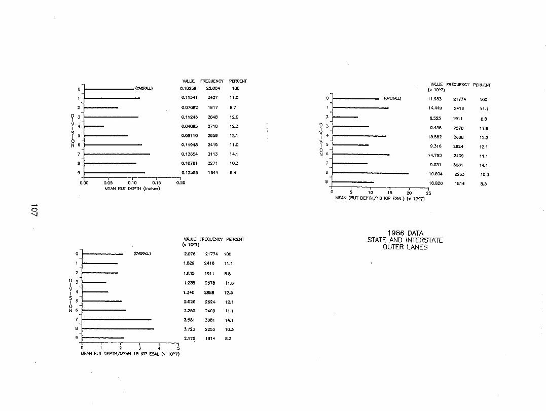
V,6LUE FREQUENCY PERCENT
OJ (0IIEAA.l.) 0.10259 22,004 100
0.11541 2427 11.0
2 0.07082 1917 8.7 -
D 3 I
0.11245 2648 12.0
V 4 I 0.04095 2710 12.3
T 5 0.09110 2659 12.1 0 N 6 0.11948 2415 11.0
7 0.13654 3113 14.1
8 0.10781 2271 10.3
9 0.12585 1844 8.4
0.00 0.05 0.10 0.15 0.20 MEAN RUT DEPTH (inches)
...... 0
"" V,6LUE FREQUENCY PERCENT
(x 10"7)
o I (0IIEAA.l.) 2.076 21774 100
1.829 2416 11.1
2 1.835 1911 8.8
D 3 I 1.238 2578 11.8
V 4 I 1.340 2688 12.3
r 5 2.026 2624 12.1 0 N 6 2.250 2409 11.1 -
7 3.581 3081 14.1
8 3.723 2253 10.3
9 2.175 1814 8.3
0 1 2 3 4 5 MEAN RUT DEPTH/MEAN 18 KIP ESAL (x 10"7)
o
2
D 3 I V 4 I
T 5
~ 6
7
8
9
V,6LUE FREQUENCY PERCENT (x 10"7)
~ (0 1.983
14.449
6.525
9.436
13.882
9.316
14.790
9.031
19.694
10.820 +1-----., ----"-----.'-----r'-----, o 5 10 15 20 25
MEAN (RUT DEPTH/l 8 KIP ESAL) (x 10"7)
1986 DATA STATE AND INTERSTATE
OUTER LANES
21774 100
2416 11.1
1911 8.8
2578 11.8
268B 12.3
2624 12.1
2409 11.1
3081 14.1
2253 10.3
1814 B.3
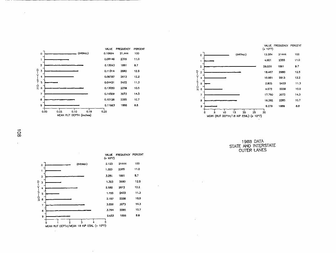
~
0 CO
OJ (CJ\IER.6I.L)
2
D 3 I Y 4 I
T 5 0 N 6
7
8
9
0.00 0.05 0.10 0.15 MEAN RUT DEPTH (Inches)
o I-~----- (CJ\IER.6I.L)
2
D 3 I Y 4
S 5 I o 6 N
7
8
9
-
VM..UE
0.10694
0.08146
0.13043
0.11314
0.09787
0.04431
0.13050
0.14509
0.10126
0.11663
0.20
VM..UE (x 10"7)
2.123
1.323
3.251
1.323
2.682
1.155
2.157
3.259
3.794
2.033
o 1 2 3 4 5
MEAN RUT DEPTH/MEAN 18 KIP ES.AJ... (x 10"7)
FREQUENCY PERCENT
21,444 100
2355 11.0
1861 8.7
2680 12.5
2613 12.2
2433 11.3
2258 10.5
3073 14.3
2285 10.7
1886 8.8
FREQUENCY PERCENT
21444 100
2355 11.0
1861 8.7
2680 12.5
2613 12.2
2433 11.3
2258 10.5
3073 14.3
2285 10.7
1886 8.8
o
2
D 3 I Y 4 I
T 5
~ 6
7
8
9
VM..UE FREQUENCY PERCENT
( CJ\IER.6I.L)
I---
I--
(x 10"7)
12.564
4.901
26.030
18.467
10.981
2.825
9.072
17.790
16.362
6.279
o 5 10 15 20 25 30 MEAN (RUT DEPTH/l B KIP ES.AJ...) (x 10"7)
1988 DATA STATE AND INTERSTATE
OUTER LANES
21444 100
2355 11.0
1861 8.7
2680 12.5
2613 12.2
2433 11.3
2258 10.5
3073 14.3
2285 10.7
1886 8.B
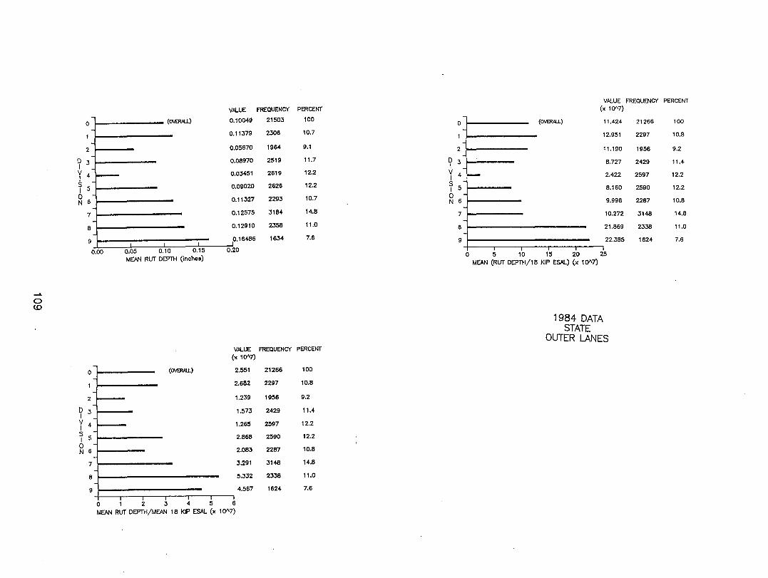
....... o <D
o
2
o 3 I V 4 I S 5 I
2 6
7
8
I--
-I
(OVERI'U.)
I I
V,ALUE
.10049 I
I
I
11379
.05670
.08970
.03451
0.09020
0.11327
0.12575
0.12910
0.16486 J
0.00 0.05 0.10 0.15 MEAN RUT DEPTH (inches)
0.20
o
2
o 3 I V 4 I
T 5
2 6
7
8
9
V,ALUE (x 10"7)
2.551
2.682
1.239
1.573 E= 1.265
2.868
2.083
3.291
5.332
4.567
0123456 MEAN RUT DEPTH/MEAN 18 KIP ESAL (x 10"7)
FREQUENCY PERCENT
21503 100
2306 10.7
1964 9.1
2519 11.7
2619 12.2
2626 12.2
2293 10.7
3184 14.8
2358 11.0
1634 7.6
FREQUENCY PERCENT
21266 100
2297 10.8
1956 9.2
2429 11.4
2597 12.2
2590 12.2
2287 10.8
3148 14.8
2338 11.0
1624 7.6
V,ALUE FREQUENCY PERCENT (x 10"7)
0 (O'lER.'l..l.) 11.424 21266 100
12.951 2297 10.8
2 11.190 1956 9.2
9 3 8.727 2429 11.4
V 4 I ~ 2.422 2597 12.2
T 5 8.160 2590 12.2
0 9.996 2287 10.8 N 6
7 10.272 3148 14.8 -
8 21.869 2338 11.0 -
9 22.385 1624 7.6
0 5 10 15 20 25 MEAN (RUT DEPTH/18 KIP ESAL) (x 10"7)
1984 DATA STATE
OUTER LANES
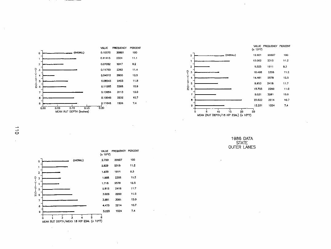
-.1.
-.1.
o
o
2
D 3 I V 4 I S 5 I
2 6
7
8
9
o
2
D 3 I
Y 4 S 5 I
2 6
7
8
9
~ ______ (0VE:R1U.)
-
0.00 0.05 0.10 0.15 MEAN RUT DEPTH (inches)
V~UE
0.10070
0.11415
0.07082
0.11765
0.04012
0.08545
0.11595
0.13654
0.10545
0.11646 J
0.20
FREQUENCY PERCENT
20801 100
2324 11.1
1917 9.2
2362 11.4
2600 12.5
2453 11.8
2266 10.9
3113 15.0
2232 10.7
1534 7.4
V~UE FREQUENCY PERCENT (x 10"7)
(0VE:R1U.) 2.720
2.629
1.835
1.888
1.718
2.815
3.028
3.581
4.475
3.220
o 1 2 3 456 MEAN RUT DEPTH/MEAN 18 KIP ES.6L (x 10"7)
20607 100
2315 11.2
1911 9.3
2306 11.2
2578 12.5
2418 11.7
2260 11.0
3081 15.0
2214 10.7
1524 7.4
0
2
9 3
V 4 I r 5 0 N 6
7
8
9
V~UE FREQUENCY PERCENT (x 10"7)
f-------- (OVEfW.L) 12.601
15.062
6.525
10.498
14.461
9.953
15.705
9.031
20.022
12.551
o 5 10 15 20 25 MEAN (RUT DEPTH/18 KIP ESAI...) (x 10"7)
1986 DATA STATE
OUTER LANES
20607 100
2315 11.2
1911 9.3
2306 11.2
2578 12.5
2418 11.7
2260 11.0
3081 15.0
2214 10.7
1524 7.4
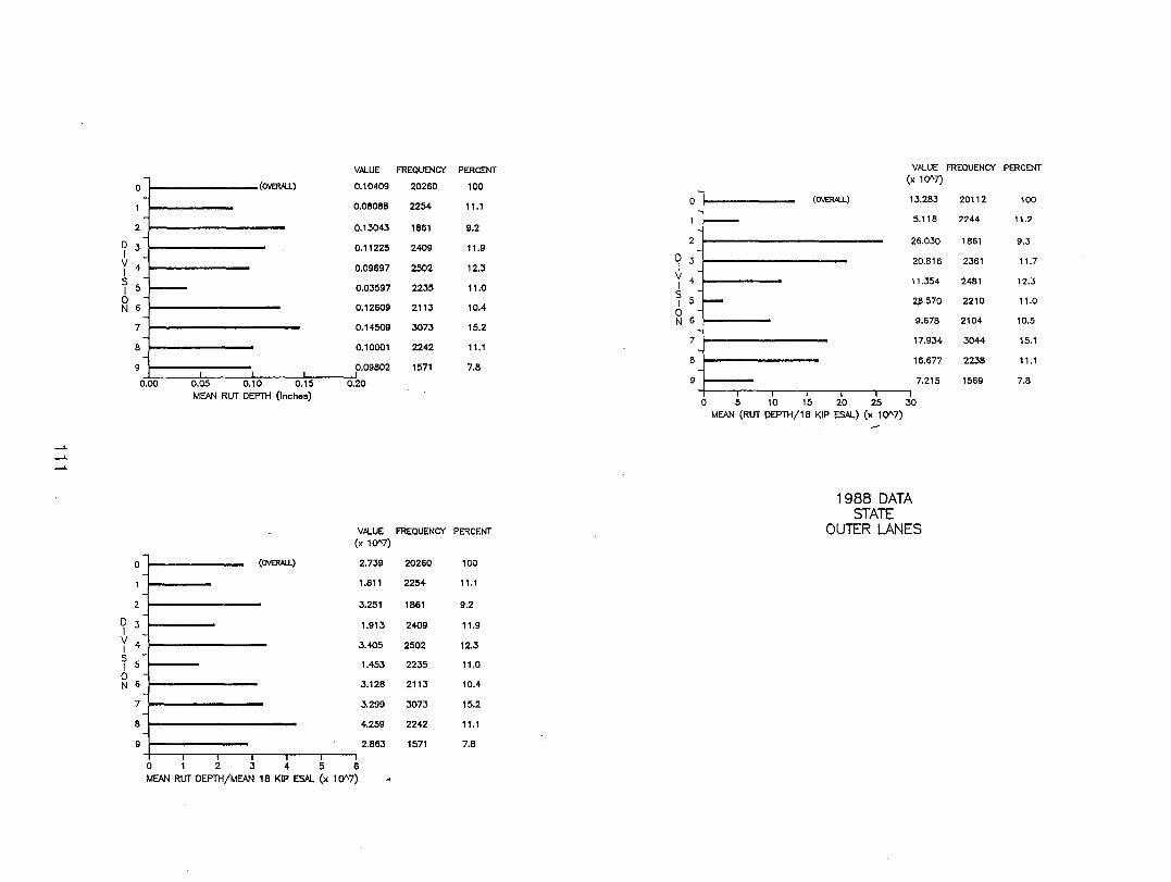
--'" --'" --'"
o
2
D 3 I V 4 I S 5 I
~ 6
7
8
9
1--------(0VERAlL)
I--
0.00 0.05 0.10 0.15 MEAN RUT DEPTH (inches)
o
2
D 3 I V 4 I
T 5
~ 6
7
8
9
(OVERAlL)
VALUE
0.10409
0.08088
0.13043
0.11225
0.09697
0.03597
0.12609
0.14509
0.10001
0.09802 J
0.20
VALUE (x 10"7)
2.739
1.811
3.251
1.913
3.405
1.453
3.128
3.299
4.259
2.863
o 1 234 5 6 MEAN RUT DEPTH/MEAN 18 KIP E5.AL (x 10"7)
FREQUENCY PERCENT
20260 100
2254 11.1
1861 9.2
2409 11.9
2502 12.3
2235 11.0
2113 10.4
3073 15.2
2242 11.1
1571 7.8
FREQUENCY PERCENT
20260 100
2254 11.1
1861 9.2
2409 11.9
2502 12.3
2235 11.0
2113 10.4
3073 15.2
2242 11.1
1571 7.8
VALUE FREQUENCY PERCENT (x 10"7)
0 (OVERAlL) 13.283 20112 100
I--- 5.118 2244 11.2
2 26.030 1861 9.3
D 3 I
20.816 2361 11.7
V 4 I 11.354 2481 12.3
T 5 ~ 2./l570 2210 11.0 0 N 6 9.678 2104 10.5
7 17.934 3044 15.1
8 16.677 2238 11.1
9 7.215 1569 7.8
0 5 10 15 20 25 30 MEAN (RUT DEPTH/18 KIP E5.AL) (x 10"7)
1988 DATA STATE
OUTER LANES
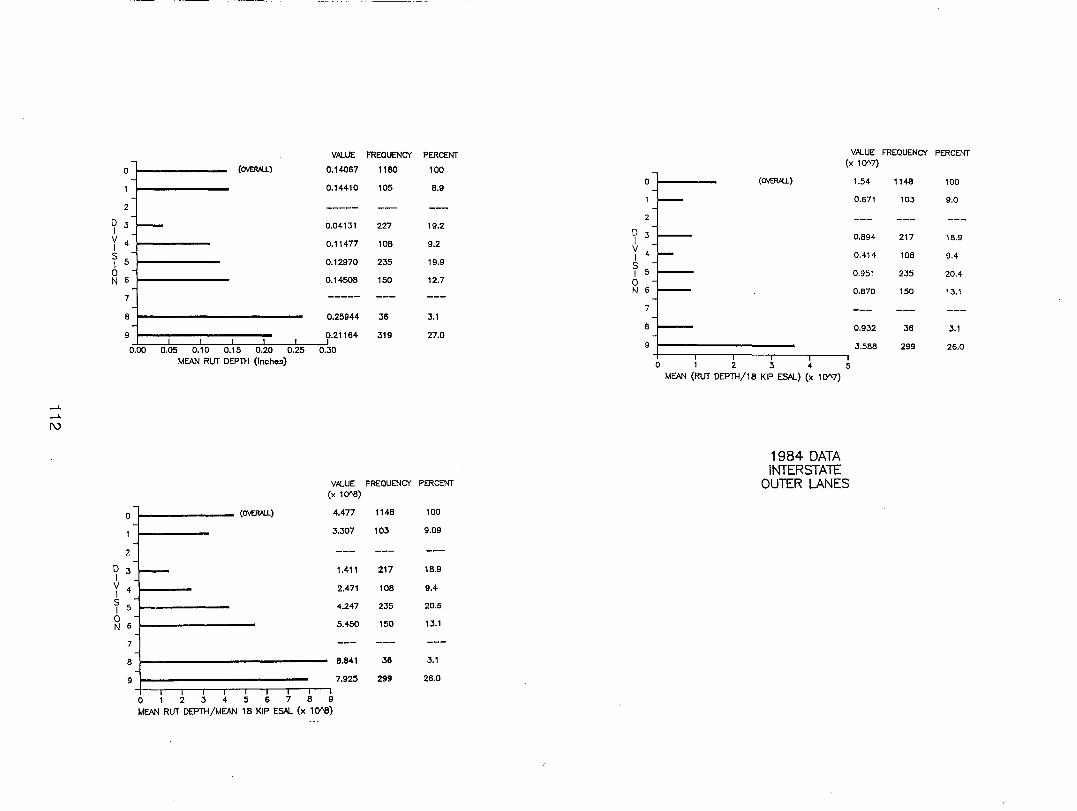
-L
-L
t\)
o
2
D 3 I V 4 I S 5 I
~ 6
7
8
9
(O\'ER.6U)
f--
VM.UE
0.14067
0.14410
0.04131
0.11477
0.12970
0.14508
0.25944
0.21164 J
0.00 0.05 0.10 0.15 0.20 0.25 0.30
o
2
D 3 I V 4 I
T 5
2 6
7
8
9
MEAN RUT DEPTH (Inches)
VM.UE (x 1 CY'B)
1------- (O\'ER.6U) 4.477
3.307
- 1.411
2.471
4.247
5.450
8.841
7.925
o 1 2 3 4 5 6 7 8 9 MEAN RUT DEPTH/MEAN 18 KIP ESAI... (x 10"8)
FREQUENCY PERCENT
1180 100
105 8.9
227 19.2
108 9.2
235 19.9
150 12.7
36 3.1
319 27.0
FREQUENCY PERCENT
1148 100
103 9.09
217 18.9
108 9.4
235 20.5
150 13.1
36 3.1
299 26.0
VM.UE FREQUENCY PERCENT (x lCY'7)
~~ (O\'ER.6U) 1.54 1148 100
0.671 103 9.0
2
?'~ 0.894 217 18.9
V 4 0.414 108 9.4 I
T 5 0.951 235 20.4 0
0.870 150 13.1 N 6
7
:s 0.932 36 3.1
3.588 299 26.0 i i i i
0 1 2 3 4 5 MEAN (RUT DEPTH/18 KIP ESAI...) (x lCY'7)
1984 DATA INTERSTATE
OUTER LANES
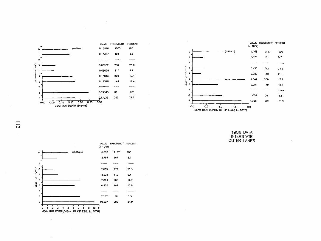
--L
--L
(J.)
o
2
o 3 I V 4 I S 5 I
2 6
7
8
9
o
2
o 3 I V 4 I
T 5
~ 6
7
8
9
(0\IER.6U.)
0.00 0.05 0.10 0.15 0.20 0.25 MEAN RUT DEPlH (Inches)
(0\IER.6U.)
r---
V.ALUE
0.13526
0.14377
0.06952
0.06056
0.15843
0.17318
0.24343
0.17236 J
0.30
V.ALUE (x 1O"B)
5.037
2.798
2.089
3.031
7.314
6.232
7.257
10.027
o 1 2 3 4 5 6 7 8 9 10 11 MEAN RUT DEPlH/MEAN 18 KIP ESftJ... (x 10"8)
FREQUENCY PERCENT
1203 100
103 8.6
286 23.8
110 9.1
206 17.1
149 12.4
39 3.2
310 25.8
FREQUENCY PERCENT
1167 100
101 8.7
272 23.3
110 9.4
206 17.7
149 12.8
39 3.3
290 24.9
V.ALUE FREQUENCY PERCENT (x 10"7)
:}= (OVffiAlL) 1.068 1167 100
0.378 101 8.7
2
rf 0.433 272 23.3
0.309 110 9.4
1.844 206 17.7
0.907 149 12.8
7
:j 1.056 39 3.3
1.726 290 24.9 I
0.0 0.5 1.0 1.5 2.0 MEAN (RUT DEPlH/18 KIP ESAL) (x 10"7)
1986 DATA INTERSTATE
OUTER LANES
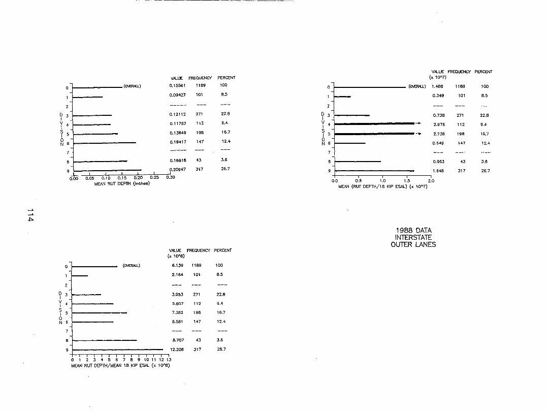
-'--'-~
o
2
D 3 I
Y 4
T 5
2 6
7
8
9
o
2
7
8
9
(O';£R,'U)
1- L
VPLUE
.15561
.09427
.12112
0.11757
0.13849
0.19417
0.16616
0.20947
0.00 0.05 0.10 0.15 0.20 0.25 0.30 MEAN RlJT DEPTH (inches)
FREQUENCY PERCENT
1189 100
101 8.5
271 22.8
112 9.4
198 16.7
147 12.4
43 3.6
317 26.7
VPLUE FREQUENCY PERCENT (x 10'8)
(0\IEI1All.) 6.139 1189
~ 2.164
3.953
5.607
7.382
5.581
8.707
12.208
o 1 2 3 4 5 6 7 B 9 10 11 12 13 MEAN RlJT DEPTH/MEAN 18 KIP E5.AL (x 1O"B)
101
271
112
198
147
43
317
100
8.5
22.8
9.4
16.7
12.4
3.6
26.7
o
2
o 3 I V 4 I S 5 I
2 6
7
8
9
VPLUE FREQUENCY PERCENT
~----------------(~ -
- - ---
(x 10"7)
1.488
0.349
0.738
2.976
2.738
0.649
0.963
1.648
0.0 0.5 1.0 1.5 2.0 MEAN (RlJT DEPTH/18 KIP E5.AL) (x 10"7)
1988 DATA INTERSTATE
OUTER LANES
1189 100
101 8.5
271 22.8
112 9.4
198 16.7
147 12.4
43 3.6
317 26.7

DATA SORTED BY MIX TYPE
115 .
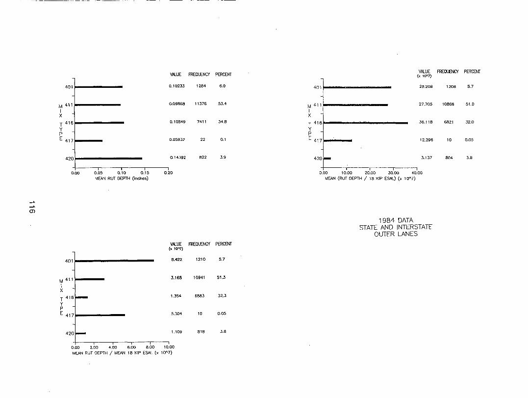
V.AlUE FREQUENCY PERCENT V.AlUE FREQUENCY PERCENT (x 10'7)
4011 0.10233 1284 6.0 40~ 29.208 1208 5.7
0.09868 11376 53.4 27.705 10866 51.0 M 411 M 411.
1 ·1 1
X - X
T 416 0.10549 7411 34.8 T 4161 36.118 6821 32.0
Y Y p P E 417 0.05932 22 0.1 E 4171 12.296 10 0.05
420 0.14392 822 3.9 420r-
3.137 804 3.8
I I I I 0.00 0.05 0.10 0.15 0.20 0.00 10.00 20.00 30.00 40.00
MEAN RUT DEPTH (inches) MEAN (RUT DEPTH / 18 KIP ESAI..) (x 1 CY'7)
-L
-L
en 1984 DATA
STATE AND INTERSTATE OUTER LANES
V.AlUE FREQUENCY PERCENT (x 10'7)
40~ 8.422 1210 5.7
3.168 10941 51.3 M 411
1 X
1.354 6883 32.3
5.304 10 0.05
1.109 818 3.8
0.00 2.00 4.00 6.00 8.00 10.00
MEAN RUT DEPTH / MEAN 18 KIP ESN.. (x 1 CY'7)
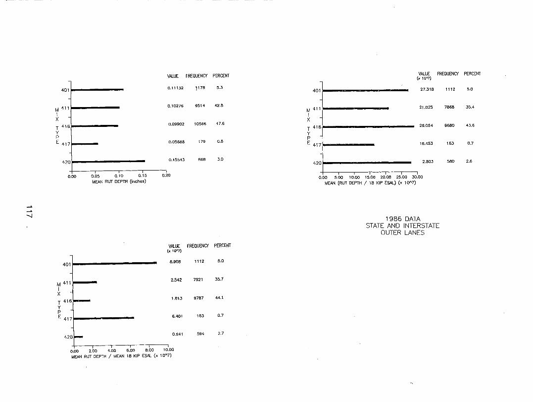
VPLUE FREQUENCY PERCENT VPLUE FREQUENCY PERCENT (x 10'7)
4011 0.11132 ]178 5.3
401l 27.318 1112 5.0
M 411 0.10276 9514 42.8
M 4111 21.025 7868 35.4
I I X X T 416
0.09902 10566 47.6 T 416
1 29.054 9680 43.6
Y Y P E 417 0.05688 179 0.8
P E 4171 16.453 163 0.7
4201 0.15543 668 3.0
4201 2.803 580 2.6
1 0.00 0.05 0.10 0.15 0.20
MEAN RUT DEPTH (inches) 0.00 5.00 10.00 15.00 20.00 25.00 30.00
MEAN (RUT DEPTH / 18 KIP ESI>J...) (x 10'7)
--'---'--.....J 1986 DATA
STATE AND INTERSTATE OUTER LANES
VPLUE FREQUENCY PERCENT (x 10'7)
40~ 8.908 1112 5.0
2.542 7921 35.7 M 411
I X
1.813 9787 44.1
6.401 163 0.7
420r 0.941 594 2.7
I I I I I 0.00 2.00 4.00 6.00 8.00 10.00
MEAN RUT DEPTH / MEAN 18 KIP ESM.. (x 10'7)
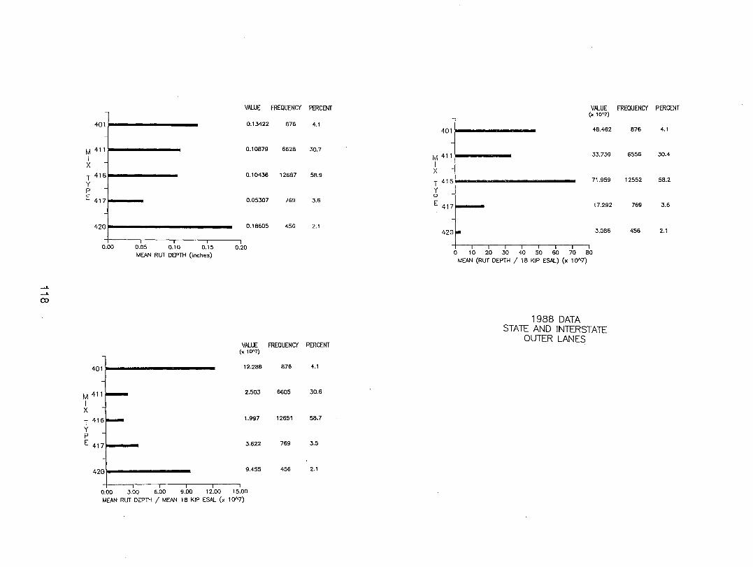
V.AJ...UE FREQUENCY PERCENT V.AJ...UE FREQUENCY PERCENT (x 10"7)
4011 0.13422 876 4.1 4011 48.462 876 4.1
M 411 0.10879 6628 30.7 M 4111 33.739 6556 30.4
1
;~ 1 x T 416 0.10436 12687 58.9
71.959 12552 58.2 T 416. Y P Y
P E 417 0.05307 769 3.6 E 4171 17.292 769 3.6
4201 0.18605 456 2.1 420 I,. 3.086 456 2.1
I I I I 0.00 0.05 0.10 0.15 0.20
a 10 20 30 40 50 60 70 80 MEAN RUT DEPTH (inches) MEAN (RUT DEPTH / 18 KIP ES/>J...) (x 10"7)
-L
-L
ex>
1988 DATA STATE AND INTERSTATE
V.AJ...UE FREQUENCY PERCENT OUTER LANES
(x 10"7)
"L 12.288 876 4.1
2.503 6605 30.6 M 411
1 X
1.997 12651 58.7
3.622 769 3.5
420' 9.455 456 2.1
0.00 3.00 6.00 9.00 12.00 15.00 MEAN RUT DEPTH / MEAN 18 KIP ESAI... (x 10"7)
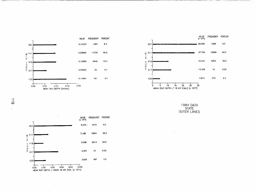
VPlUE FREQUENCY PERCENT VPlUE FREQUENCY PERCENT (x 10'7)
401 0.10233 1284 6.4 401l 29.208 1208 6.0
. I
0.09868 11376 56.6 l 27.705 10866 54.0
M 411 !vi 411 ,
I X ~ X
T 416 0.10090 6542 32.5 T 416j 10.519 5952 29.6
Y Y ,
p t 41~ E 417 0.05932 22 0.1 12.296 10 0.05
I
420, 0.14604 491 2.4 4+_ 4.813 473 2.4
1 I I I I I I 0.00 0.05 0.10 0.15 0.20 a 5 10 15 20 25 30
MEAN RUT DEPTH (inches) MEAN (RUT DEPTH / 18 KIP E5.AL) (x 10"7)
--'---'-CD
1984 DATA STATE
OUTER LANES
VPlUE FREQUENCY PERCENT (x 10'7)
40~ 8.422, 1210 6.0
3.168 10941 54.4 M 411
I X 416L- 2.068 6014 29.9
T Y p
E 417' 5.304 10 0.05
420\ 2.529 487 2.4
I I I I I 0.00 2.00 4.00 6.00 8.00 10.00
MEAN RUT DEPTH / MEAN 18 KIP ESAL (x 1()1\7)
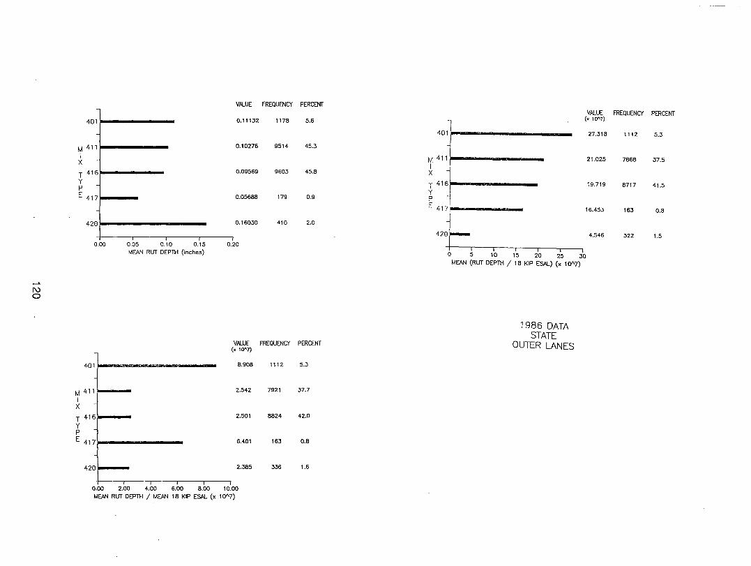
....... N o
V.AlUE
~t= 0.11132
M 411 0.10276
I X
T 4161 0.09569
Y P
E "l 0.05688
0.16030 420
I I 0.00 0.05 0.10 0.15 0.20
MEAN RUT DEPTH (inches)
V.AlUE (x 10"7)
401L ........ ,, ____ 8.908
1 2.542 tv1 411' -
I X
T 4161 2.501
Y p E 417 6.401
420 2.385
, I 0.00 2.00 4.00 6.00 8.00 10.00
MEAN RUT DEPTH / MEAN 18 KIP ESAL ex 10"7)
FREQUENCY PERCENT
1178 5.6
9514 45.3
9603 45.8
179 0.9
410 2.0
FREQUENCY PERCENT
1112 5.3
7921 37.7
8824 42.0
163 0.8
336 1.6
V.AlUE
4011 (x 10"7)
: 27.318
M ",i 21.025
~ 1 19.719 ~ 416
1
~ 1 :: 417: 16.453
1 4.546
42°t=1 I I I I I
o 5 10 15 20 25 30 MEAN (RUT DEPTH / 18 KIP ESAL) ex 10"7)
1986 DATA STATE
OUTER LANES
FREQUENCY PERCENT
1112 5.3
7868 37.5
8717 41.5
163 0.8
322 1.5
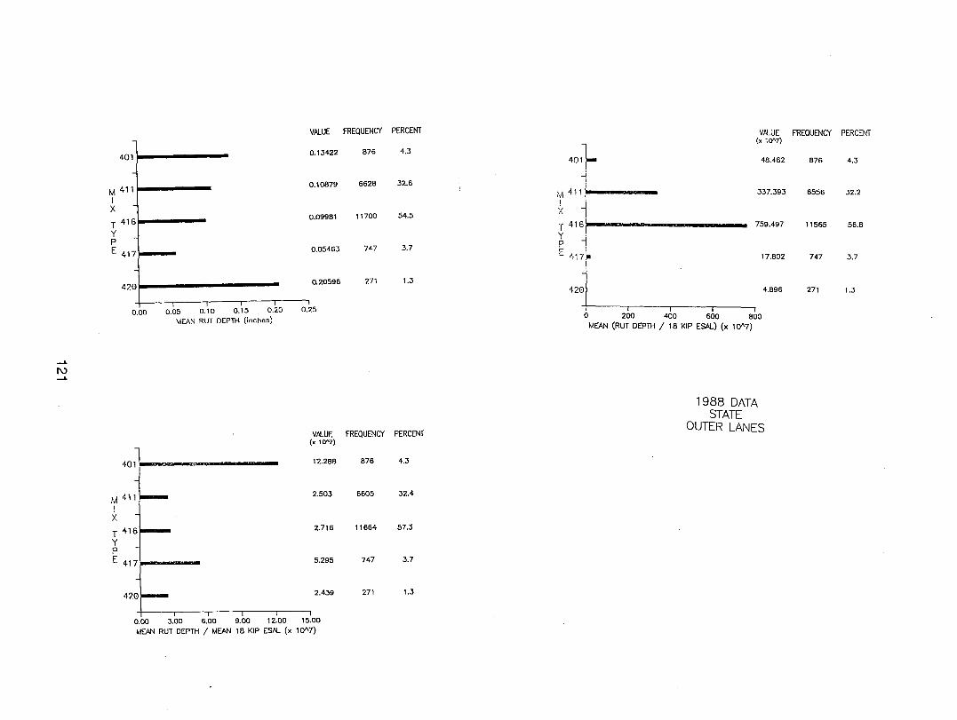
V.AlUE FREQUENCY PERCENT V.AlUE FREQUENCY PERCENT (x 10'7)
0.13422 876 4.3 401""}-
401} 48.462 876 4.3
-i 6628 32.6 I
0.10879 I M 411 M 411; 337.393 6556 32.2 I I 1 X
54.5 X 0.09981 11700
T 4161
T 416 .. 759.497 11565 56.8 Y Y . P
0.05463 747 3.7 P 1 E 417 E 417 '. 17.802 747 3.7
I
0.20596 271 1.3 "l 420} 4.896 271 1.3
0.15 0.20 0.25 I --,.- I I 0.00 0.05 0.10 0 200 400 600 800 MEAN RUT DEPTH (inches)
MEAN (RUT DEPTH / 18 KIP ESAl..) (x 10"'7)
-L
I\) -L
1988 DATA STATE
V.AlUE FREQUENCY PERCENT OUTER LANES
(x 10'7)
l 401' r ....
,,41L !r-X
~ 416
E 417
42~, , , ,'~"
1'2.288 876 4.3
2.503 6605 32.4
2.716 11664 57.3
5.295 747 3.7
271 1.3
0.00 3.00 6.00 9.00 12.00 15.00 MEAN RUT DEPTH / MEAN 18 KIP ESAI... (x 10"'7)
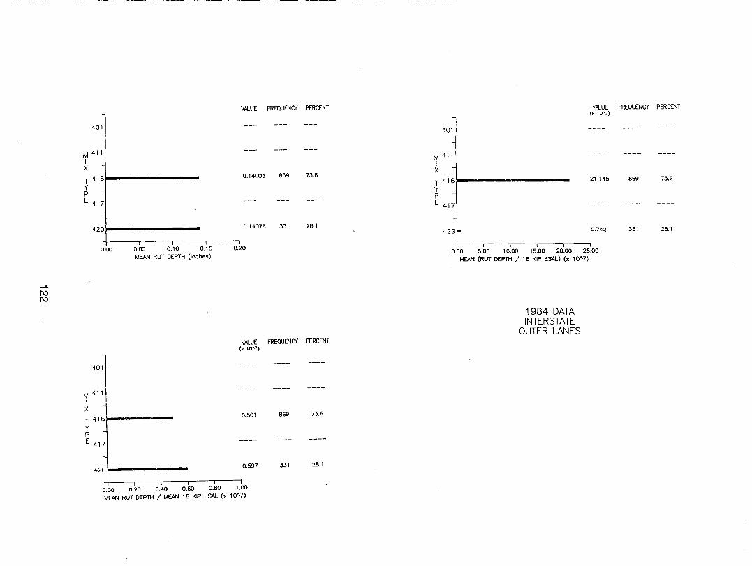
-L
I\) I\)
4011
M 411
1 X T 416
Y P E 417
4201
0.00 0.05 0.10 0.15
MEAN RUT DEPTH (inches)
401l
~ ,,411\ .; i
:-: 1 T 416~\o-----Y p E 417
4201-1 ------
VM..UE FREQUENCY PERCENT
0.14003 869 73.6
0.14076 331 28.1
0.20
VM..UE FREQUENCY PERCENT (x 'Q/'7)
0.501 869 73.6
0.597 331 28.1
0.00 0.20 0.40 0.60 0.80 1.00 MEAN RUT DEPTH / MEAN 1 B KIP ESM.. (x 10"7)
VM..UE (x 'Q/'7)
401l
~ M 411 1 X T 416 1 21.145
Y P E 417
I
4201 0.742
+---r- I I I I 0.00 5.00 10.00 15.00 20.00 25.00
MEAN (RUT DEPTH / 18 KIP ESM..) (x 10"7)
1984 DATA INTERSTATE
OUTER LANES
FREQUENCY PERCENT
869 73.6
331 28.1
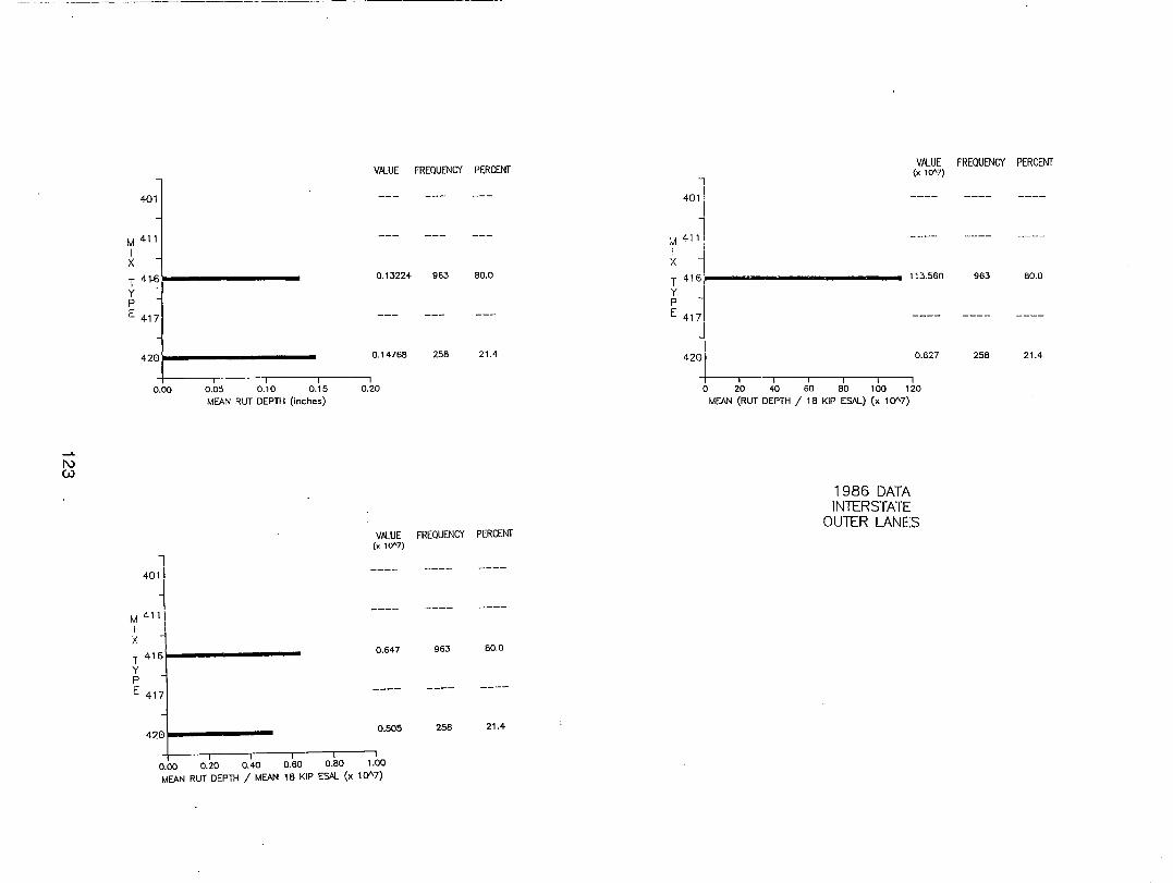
FREQUENCY PERCENT VALUE FREQUENCY PERCENT VALUE (x lCJ1'7)
l 4011 401
1
l M 411 :,.1 411!
1 ~ X X
T 41-6 0.13224 963 80.0
r~ 113.560 963 80.0
Y p
E 417 E 417
"L 4201 0.14768 258 2104 0.627 258 21.4
I I I I I 0.00 0.05 0.10 0.15 0.20 0 20 40 60 80 100 120
MEAN RUT DEPTH (inches) MEAN (RUT DEPTH / 18 KIP ESAL) (x 10"7)
...... I\) w
1986 DATA INTERSTATE
OUTER LANES VALUE FREQUENCY PERCENT
(x lCJ1'7)
l 4011
~ M 4111 I I
"of
,. 416 1 0.647 963 80.0
T '( P E 417
42~ 0.505 258 21.4
I I I I I 0.00 0.20 0040 0.60 0.80 1.00
MEAN RUT DEPTH / MEAN 18 KIP ESAL (x 10"7)
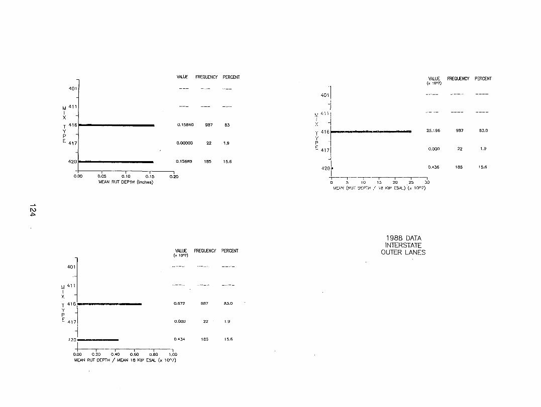
-" I\) .p.
V,6lUE FREQUENCY PERCENT
l 401
M 411 I X
T 4161 0.15840 987 83
Y P
E 41~ 0.00000 22 1.9
0.15689 185 15.6 420
I 0.00 0.05 0.10 0.15 0.20
MEAN RUT DEPTH (inches)
V,6lUE FREQUENCY PERCENT (x 10"7)
401
M 411 I X
I
~ 41~i 0.672
~ 417~ 0.000
~20 0434
I I ,---,- I I I
0.00 0.20 0.40 0.60 0.80 1.00
MEAN RUT DEPTH / MEAN 18 KIP ESAL ex 10"7)
967 83.0
22 1.9
185 15.6
V,6lUE FREQUENCY PERCENT
40~ \,411 i .J. I
.~ ~ ~ 416)oo~------'( I p l E 4171
I I
l 42(H
I
(x 10"7)
25.196
0.000
0.436
+----r---.~ [ I I I o 5 10 15 20 25 30
MS!~ (RUT D::?,i-1 .' 18 KIP ES,oL) (x 10"7)
1988 DATA INTERSTATE
OUTER LANES
987 83.0
22 1.9
185 15.6
FREQUENCY DISTRIBUTIONS
125 .
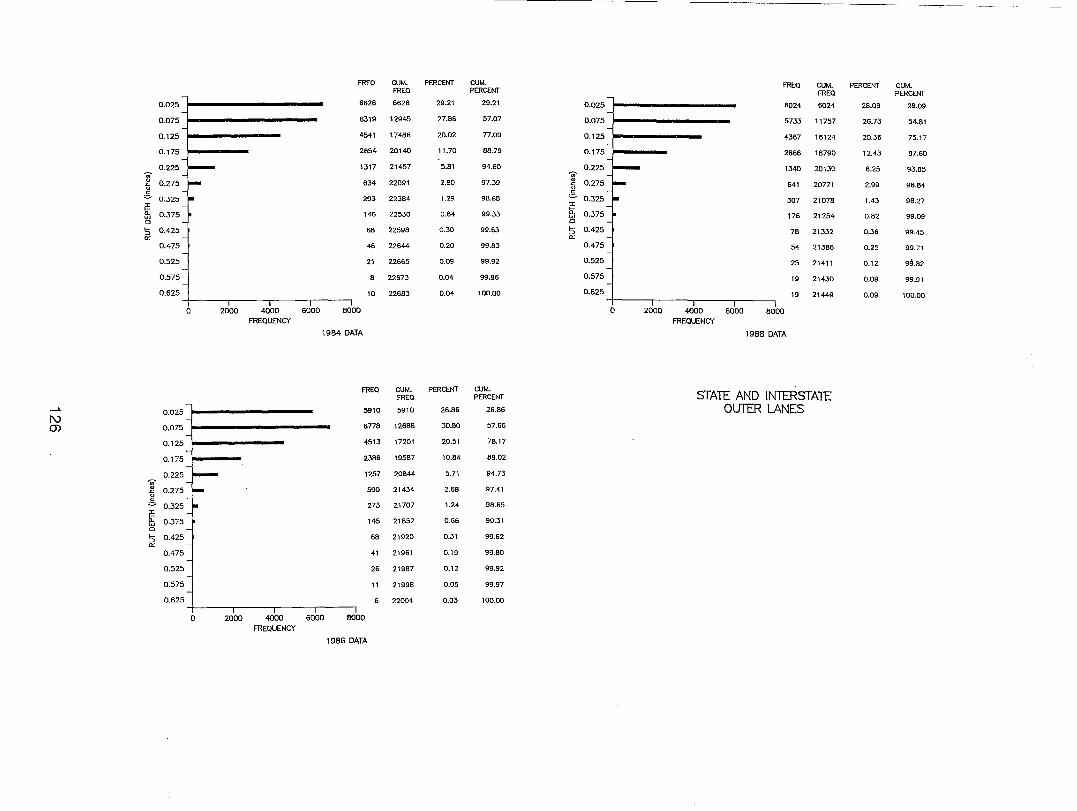
FREO CUM. PERCENT CUM. FREO CUM. PERCENT CUM. FREO PERCENT FREO PERCENT
0.025 6626 6626 29.21 29.21 0.025 6024 6024 28.09 28.09
0.075 6319 12945 27.86 57.07 0.075 5733 11757 26.73 54.81
0.125 4541 17486 20.02 77.09 0.125 4367 16124 20.36 75.17
0.175 2654 20140 11.70 88.79 0.175 2666 18790 12.43 87.60 -21457 5.81 94.60 0.225 0.225 ~ 1317 1340 20130 6.25 93.85 ,..,. - ,..,.
Q) 0.275 ~ 0.275 r- 634 22091 2.80 97.39 -5 641 20771 2.99 96.84
g - c: Co 0.325 ~ 293 2238' 1.29 98.68 Co 0.325 307 21078 1.43 98.27 i!: - i!: a. 0.375 146 22530 0.64 99.33 fu 0.375 176 21254 0.82 99.09 1.01
0 0 -l-I-- 0.425 68 22598 0.30 99.63 OJ 0.425 78 21332 0.36 99.45 OJ - '" 0:
0.475 46 22644 0.20 99.83 0.475 54 21386 0.25 99.71
0.525 21 22665 0.09 99.92 0.525 25 21411 0.12 9~.82 -0.575 8 22673 0.04 99.96 0.575 19 21430 0.09 99.91
0.625 10 22683 0.04 100.00 0.625 19 21449 0.09 100.00
0 2000 4000 6000 BOOO 0 2000 4000 6000 BOOO FREQUENCY FREQUENCY
1984 DATA 1988 DATA
FREQ CUM. PERCENT CUM. STATE AND INTERSTATE FREO PERCENT
...... 0.025 5910 5910 26.86 26.86 OUTER LANES I'V (J) 0.075 6778 12688 30.80 57.66
0.125 4513 17201 20.51 78.17
0.175 2386 19587 10.84 89.02
0.225 1257 20844 5.71 94.73
'if -5 0.275 590 21434 2.68 97.41
.5. 0.325 273 21707 1.24 98.65
i!: fu 0.375 145 21852 0.66 99.31 0
I- 0.425 68 21920 0.31 99.62 OJ 0::
0.475 41 21961 0.19 99.80
0.525 26 21987 0.12 99.92
0.575 11 21998 0.05 99.97
0.625 6 22004 0.03 100.00
0 2000 400D 6000 BODO FREQUENCY
19B6 DATA
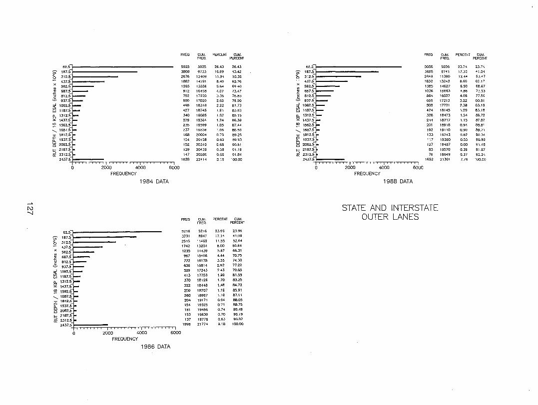
FREQ CUM. PERCENT CUM. FREQ CUM. PERCENT CUM. FREQ. PERCENT FREe. PERCEN.
62.5 5925 5925 26.43 26.43 62.5 5056 5056 23.74 23.74
t 187.5 3808 9733 16.99 43.42 t 187.5 3685 8741 17.30 41.04
312.5 2676 12409 11.94 55.36 312.5 2649 11390 12.44 53.47
437.5 1882 14291 8.40 63.76 437.5 1852 13242 8.69 62.17 x
562.5 en 1265 15556 5.64 69.40 X
562.5 en 1385 14627 6.50 68.67 Q) 687.5 912 16468 4.07 73 .• 7 Q) 687.5 1036 15663 4.86 73.53 .c .c u 812.5 752 17220 3.36 76.83 u 812.5 864 16527 4.06 77.59 c 5 Co 937.5 600 17620 2.68 79.50 937.5 686 17213 3.22 80.81
~ 1062.5 498 18318 2.22 81.73 ~ 1062.5 508 17721 2.38 83.19
w 1187.5 427 18745 1.91 83.63 w 1187.5 424 18145 1.99 85.18
0.. 1312.5 340 19085 1.52 85.15 0.. 1312.5 328 18473 1.54 86.72 SO 1437.5 279 19364 1.24 86.39 SO 1437.5 244 18717 1.15 87.87 to 1562.5 235 19599 1.05 87.44 to 1562.5 201 18918 0.94 88.81
'-. 1687.5 237 19836 1.06 88.50 '-. 1687.5 192 19110 0.90 89.71
~ 1812.5 168 20004 0.75 89.25 ~ 1812.5 133 19243 0.62 90.34
0.. 1937.5 154 20158 0.69 89.93 0.. 1937.5 117 19360 0.55 90.89
~ 2062.5 152 20310 0.68 90.61 ~ 2062.5 127 19487 0.60 91.48
f-- 2187.5 129 20439 0.58 91.19 f-- 2187.5 83 19570 0.39 91.87
iE 2312.5 147 20586 0.66 91.8.l. iE 2312.5 79 19649 0.37 92.24 1828 22414 8.:6 100.00 2437.5 1652 21301 7.76 100.00
I I iii iii iii I' i iii
0 2000 4000 6000 0 2000 4000 6000 FREQUENCY FREQUENCY
1984 DATA 1988 DATA
-'-STATE AND INTERSTATE I\)
-.....J OUTER LANES FREe CUM. PERCENT CUM.
FREQ. PERCENT
62.5 5216 5216 23.96 23.96
t 187.5 3731 8947 17.14 41.09
312.5 2515 11462 11.55 52.64
437.5 1742 13204 8.00 60.64 X
562.5 1235 14439 5.67 66.31 en 967 15406 4.44 70.75 Q) 687.5 .c
772 16178 3.55 74.30 u 812.5 c Co 937.5 636 16814 2.92 77.22
~ 1062.5 529 17343 2.43 79.65
413 17756 1.90 81.55 w 1.70 83.25
0.. 370 18126
SO 322 18448 1.48 84.72
to 259 18707 1.19 85.91 260 18967 1.19 87.11
, '.'~~ 204 19171 0.94 88.05
154 19325 0.71 88.75 i::J 1937.5 161 19486 0.74 89.49 o 2062.5
~ 2187.5 153 19639 0.70 90.19
"" 2312.5 137 19776 0.63 90.82
1998 21774 9.18 100.00 I
0 2000 4000 6000
FREQUENCY
1986 DATA
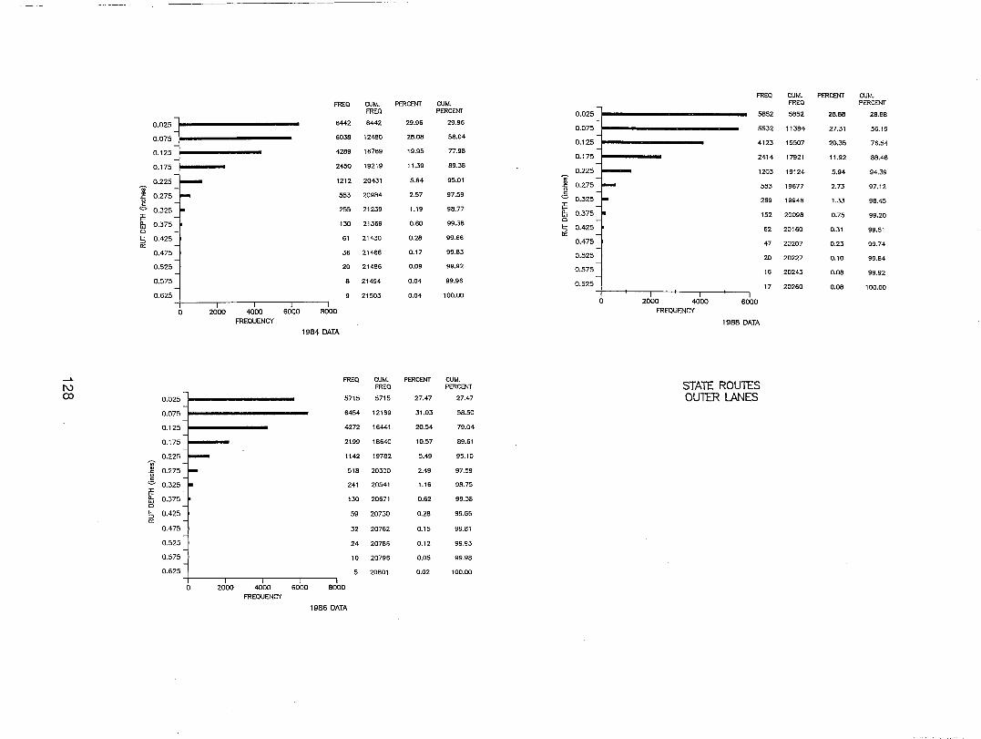
FREQ CUM. PERCENT CUM. FREQ CUM. PERCENT CUM. FREQ PERCENT
FREQ PERCENT 0.025 5852 5852 28.BB 28.88 -
6442 6442 29.96 29.96 0.075 5532 11384 27.31 56.19
0.025 -
6038 12480 28.08 58.04 0.125 4123 15507 20.35 76.54
0.075 -
4289 16769 19.95 77.98 2414 17921 11.92 88.46
0.125 0.175 -
2450 19219 11.39 89.38 1203 19124 5.94 94.39
0.175 0.225 -
1212 20431 5.64 95.01 ]' 0.275 553 19677 2.73 97.12 0.225 t"'-
o -;;;- -20984 2.57 97.59 c: " 0.275 !- 553 '=' 0.325 269 19946 1.33 98.45
.c: 0
;E c: 255 21239 1.19 98.77
0.75 99.20 '=' 0.325 r- fu 0.375 152 20098 ;E - a fu 0.375 130 21369 0.60 99.38
1:3 0.425 62 20160 0.31 99.51 a -'" 61 214.30 0.28 99.66
0.475 47 20207 0.23 99.74 1:3 0.425
'" 36 21466 0.17 99.83 0.525 20 20227 0.10 99.84
0.475
0.525 20 21486 0.09 99.92 0.575 16 20243 0.08 99.92
0.575 8 21494 0.04 99.96 0.525 17 20260 0.08 100.00 0.525 9 21503 0.04 100.00
0 2000 4000 6000
8600 FREQUENCY 0 2000 4000 6000
FREQUENCY 1988 DATA
1984 DATA
--L FREQ CUM. PERCENT CUM. I\.) FREQ PERCENT STATE ROUTES ex> 0.025 5715 5715 27.47 27.47 OUTER LANES
0.075 6454 12169 31.03 58.50
0.125 4272 16441 20.54 79.04
0.175 2199 18640 10.57 89.61
0.225 -;;;- I-- 1142 19782 5.49 95.10
" 0.275 ro- 518 20300 2.49 97.59 -5 c:
r-'=' 0.325 241 20541 1.16 98.75 ;E 0. 0.375 130 20671 0.62 99.38 w a f- 0.425 59 20730 0.28 99.66 :J
'" 0.475 32 20762 0.15 99.81
0.525 24 20786 0.12 99.93
0.575 10 20796 0.05 99.98
0.625 5 20801 0.02 100.00
0 2000 4000 6000 8000 FREQUENCY
1986 DATA
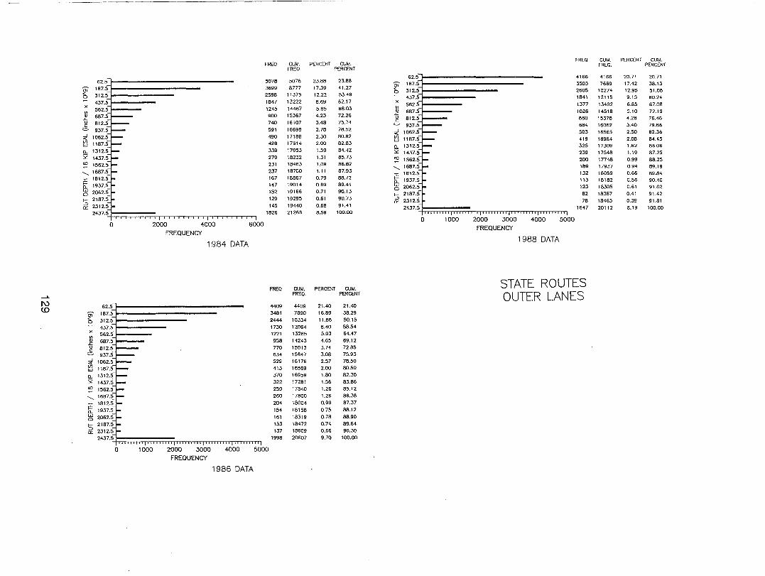
--'-
'" <D
m 1~~~~~============-----CS 312.51'". -------
437.5 r-----"' " .r:; u ~
~ w 0... ;;;; <0
562.5JI----687.5
'- 1687.5 I 1812.S b: 1937.S ::g 2062.5 I- 2187.5
~ 2312.5
2437.S~q~:;::;::;::;::;:;:~::,.-r-r-r""-TTT"T"""-~ __
a 2000 4000 6000 FREQUENCY
1984 DATA
f ~;H1t::::===========:----437.SQr. ------
"' " .r:; u S
~ W
0... ;;;; <0
"""--
j:!: 0... W o
562.511-----
~ 2312.5
2437.Sl, , , , , , , , , " , , , , , , , , " , , , , , , , , " , , , , , , , , " , , , , , , , , ,
FREO CUM. PERCf:NT CUM. FREQ. ;:>ERCENT
5078 5078 3699 8777 2598 11375
1847 13222 1245 14467 900 15367 740 16107 591 16698 490 17188 426 17614
339 17953 279 18232 231 18463 237 18700 167 18867 147 19014 152 19166 129 19295 145 19440
1826 21266
23.88 17.39
12.22
8.69 5.85 4.23 3.48 2.78 2.30 2.00 1.59 1.31
1.09 1.11 0.79 0.69 0.71 0.61 0.68 8.59
23.88 41.27
53.49 62.17 68.03 72.26 75.74 78.52 80.82 82.83 84.42 85.73 86.82 87.93 88.72 89.41 90.13 90.73 91.41
100.00
FREQ CUM. PERCENT CUM. FREQ. PERCENT
4409 4409 21.40 21.40 3481 7890 1 6.89 38.29 2444 10334 11.86 50.15 1730 12064 8.40 58.54 1221 13285 5.93 64.47
958 14243 4.65 69.12
770 15013 3.74 72.85 634 15647 3.08 75.93 529 16176 2.57 78.50 413 16589 2.00 BO.50
370 16959 1.80 82.30 322 17281 1.56 83.86
259 17540 1.26 85.12 260 17800 1.26 86.38 204 18004 0.99 87.37
154 18158 0.75 88.12
161 18319 0.78 88.90 153 18472 0.74 89.64 137 18609 0.66 90.30
1998 20607 9.70 100.00
a 1000 2000 3000 FREQUENCY
4000 5000
1986 DATA
m l~~··~~E~~~====:--CS 312.5. 437.5
562.5 ,..-----~ 687.~1J-----I 812.5
~ w 0... ;;;; <0
'I 1812.S t 1937.S ::g 2062.5 I- 2187.5 ~ 2312.5
2437,Sl. iii i I I i I I' , , i , ill I Iii I I I I iii II iii iii i I II iii iii I i I a 1000 2000 3000
FREQUENCY 4000 5000
1988 DATA
FREQ CUM. PERCENT CUM. FREO. PERCENT
4166 4166 20.71 20.71 3503 7669 17.42 38.13 2605 10274 12.95 51.08 1841 12115 9.15 60.24
1377 13492 6.85 67.08
1026 14518 5.10 72.19 860 15378 4.28 76.46
684 16062 3.40 79.86
503 16565 2.50 82.36 419 16984 2.08 84.45 325 17309 1.62 86.06
239 17548 1.19 87.25 200 17748 0.99 88.25 189 17937 0.94 89.19 132 18069 0.66 89.84 113 18182 0.56 90.40 123 18305 0.61 91.02
82 18387 0.41 91.42
78 18465 0.39 91.81 1647 20112 8.19 100.00
STATE ROUTES OUTER LANES
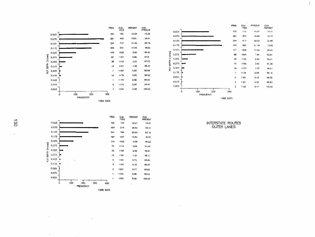
FREQ CUM. PERCENT CUM. FREQ CUM. PERCENT CUM.
~ ~ 1 ~ ~ 0.025 ~ 184 184 15.59 '5.59 0.025 ,72 '72 '4.47 14.47
0.075 281 465 23.81 39.4' 0.075 20, 373 16.90 31.37
0.125 252 717 21.36 .60.76 0.1:5 ~ 244 617 20.52 51.89
0.175 _ 204 921 17.29 78.05 0.1.5 252 869 21.'9 ;'3.09
0.225 105 1026 8.90 86.95 ... 0.225 --l 137 '006 , 1.52 8".61 w m .£ 0.275 81 1107 6.86 93.81 g 0.275 88 1094 7.40 92.01
oS _ Co 0325 i 0.325 38 1145 3.22 97.03 iE . 38 1132 3.20 95.21
~ 0.375 ~ 16 1161 1.36 98.39 ~ 0.375 24 1156 2.02 97.22
1- 0425 L !:; 0.425 ~. '" 7 1168 0.59 98.98 It: 16 "72 1.35 98.57
0.475 ~ ,0 ,,78 0.85 99.83 OA75 "79 0.59 99.16
0.525 1'79 0.08 99.92 0.525 5 , '84 0.42 99.58
0575 0.575 . _ 0 , ,79 0.00 99.92 ' '87 0.25 99.83
0.625 1'80 0.08 '00.00 0.625 "89 O.;? '00.00
+--------.r--------~I--------, I I I o 100 200 300 0 100 200 300
FREQUENCY FREQUEI~CY 1984 DATA 1988 DATA
FREQ CUM. PERCENT CUM. -l. FREQ PERCENT .
IN1ERSTA1E ROU1ES w 0.025 195 '95 '6.2' '6.21 0
0.075 - OU1ER LANES 324 5,9 26.93 43.14
0.125 241 760 20.03 63.'8
0.175 '87 947 '5.54 78.72
0.225 115 '062 9.56 88.28 ]' -~ 0
0.275 72 ,134 5.99 94.26 c = 0.325 ~ 32 , ,66 2.66 96.92 i!' fu 0.375 ~ ,5 118, 1.25 98.';' a 1- 0.425 ::l 9 It:
1190 0.75 98.92
0.475 9 '199 0.75 99.67
0.525 2 1201 0.,7 99.83
0.575 '202 0.08 99.92
0.625 1203 0.08 '00.00 I
0 100 200 300 400 FREQUENCY
1986 DATA
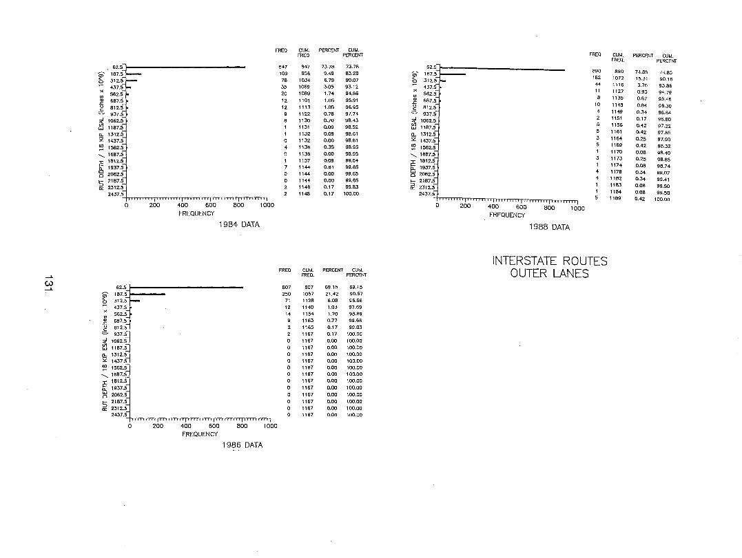
....... W .......
f )(
en Q) .c u c
687.5 812.5
:..:;... 937.5
~ 1062.~ w 1187.5 !h 1312.5 ::.: 1437.$ OJ 1562.$
'- 1687.$
F 1812.~ a.. 1937.5 ~ 2062.$
'3 2187.~ 0:: 2312.5
2437.$ IIIII""., •• I'i, •• llli.i.!.!il"li.lllljil •• !.i.lj
o 200 400 600 FREQUENCY
800 1000
1984 DATA
62.511-------------en 187.5 b 312.5
" Ul Q) .c o c
437.5 562.5 687.5 812.5
.:.::.. 937.5
<t. 1062.5 UJ -w 1187.5
a.. ;Z
1312.5 1437.5
~ 1562.5 '- 1687.$
F 1812.~ a.. 1937.5
~ 2062.5
'3 2187.~ 0:: 2312.5
2437.5 Ilili.',!ili!.ii, •• iili,.I ••• lli, ••• i.i!l.ii •• iii.\
FREO
847 109 78 35 20
12 12
8
o 4 o 1
7 o o 2 2
FREO
807 250
71 12 14 9
2 2 o o o o o o o o
o o o
o 200 400 600 FREQUENCY
800 1000
1986 DATA
CUM. PERCENT CUM. FRED. PERCENT
847 956
1034 1069 1089
1101 1113 1122 1130 1131 1132 1132 1136 1136 1137 1144 1144 1144 1146 1148
73.78 9.49 6.79 3.05 1.74
1.05 1.05 0.78 0.70 0.09 0.09 0.00 0.35 0.00 0.09 0.61 0.00 0.00 0.17 0.17
73.78 83.28 90.07 93.12 94.86
95.91 96.95 97.74 98.43 98.52 98.61 98.61 98.95 98.95 99.04 99.65 99.65 99.65 99.83
100.00
CUM. PERCENT CUM. FRED. PERCENT
807 1057 1128 1140 1154 1163 1165 1167 1167 1167 1167 1167 1167 1167 1167
1167 1167 1167 1167
"67
69.15 69.15 21.42 90.57
6.08 96.66 1.03 97.69 1.20 98.89 0.77 99.66 0.17 99.83 0.17 100.00 0.00 100.00 0.00 100.00 0.00 100.00 0.00 100.00 0.00 100.00 0.00 100.00 0.00 100.00
0.00 100.00 0.00 100.00 0.00 100.00 0.00 100.00 0.00 100.00
FRED
62.S .. I ________________ _
en 187.5-1 b 312.5
890 182 44 11 8
10 4 2 5 5
x en Q) .c
437.5 562.5
687.5 g 812.~ c- 937.5 <t. 1062.5 UJ -w 1187.5 a.. 1312.$ ;Z 1437.5 OJ 1562.$
'- 1687.$
F 1812.~ a.. 1937.5 w -o 2062.5 I-- 2187.$ ::> -0:: 2312.5
5
3 1
4 4
2437.$ filllll]i'jl.i ••• "lji!i""'!II •• I" ••• iil •• i •• i.1
1 5
o 200 400 600 FREQUENCY
800
1988 DATA
1000
INTERSTATE ROUTES OUTER LANES
CUM. PERCEIH CUM. FRED. PERCENT
890 1072 1116
1127 1135
1145 1149 1151 1156 1161 1164 1169 1170 1173 1174 1178 1182 1183 1184 1189
74.85 15.31
3.70
0.93
0.67 0.84 0.34 0.17 0.42 0.42 0.25 0.42 0.08 0.25 0.08 0.34 0.34 0.08 0.08 0.42
7-\.85 90.16
93.86 94.79 95.46
96.30 96.64 96.80 97.22 97.65
97.90 98.32 98.40 98.65 98.74 99.07 99.41 99.50 99.58
100.00
APPENDIX B
LAYER PROFILES FROM FIELD TEST SITES
132 .
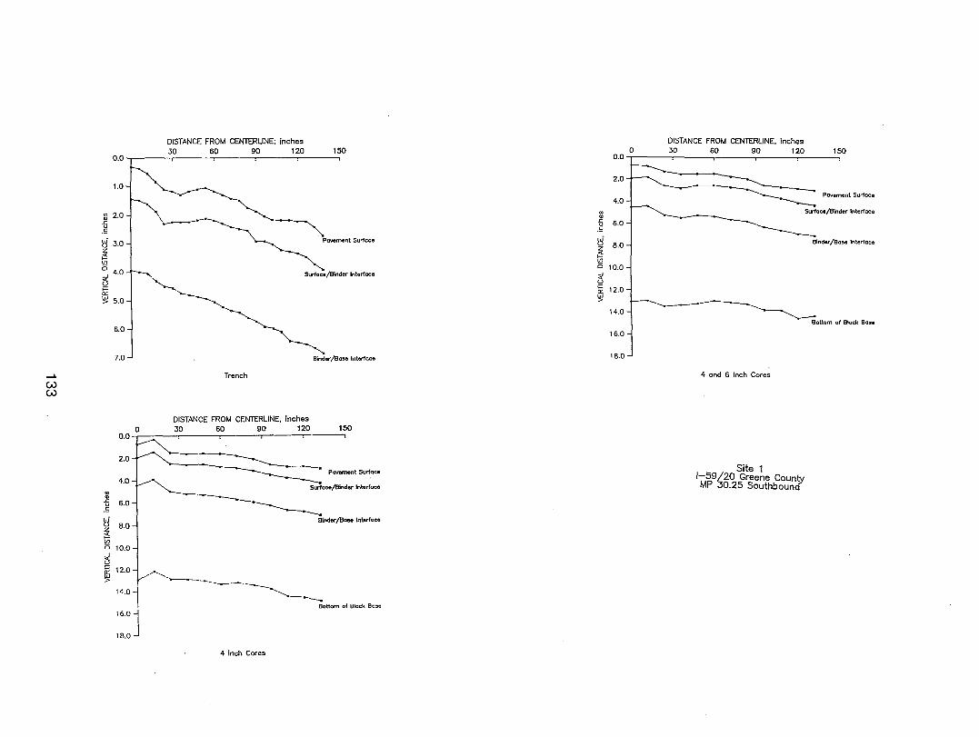
....... W W
DISTANCE FROM CENTERLINE; inches 30 60 90 120 150
M~ 1.0
:a 2.0 "\
~ .c u .s tf 3.0 PaVQment Surfoce
~ (/)
0 ~ 4.0
'----Surface/Binder Interlace
U ;= a::
~ '5' 5.0
6.0
7.0...J Binder /Boso Interlace
Trench
DISTANCE FROM CENTERLINE. inches o 30 60 90 120 150
0.0 .~
en ~ .S t.J
2.0
4.0
6.0
~ B.O
t;; o 10.0
3 ~ 12.0
'5' I
14.01 16.oj IB.O
Pavement Surface
Surface/Blnder Interface
Binder /BaH Interlace
~----------~~~ BoUom of Black Base
4 inch Cores
0.0
2.0
4.0
en
" .c 6.0 u .s t.J U B.O ~ ~ o 10.0 ~ U
~ 12.0 '5'
14.0
16.0
IB.O
0 DISTANCE FROM CENTERLINE. inches 30 60 90 120 150
4 and 6 Inch Cores
Site 1 1-59L20 Greene County MP 30.25 Southbound"
POI/amont Surface
Surface/Binder Interface
Binder/Base Interface
Bollom of Block Bose
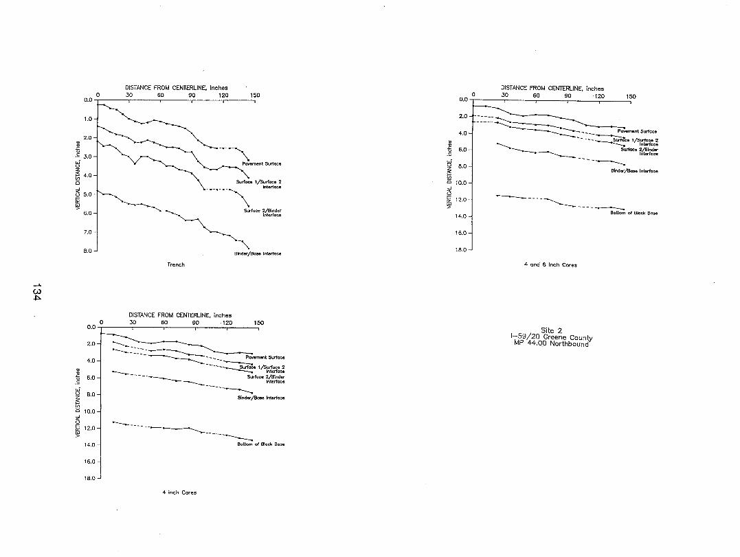
--L
W ~
'" " .s::; u
0.0
1.0
2.0
.S .1.0 W u
~ 40
DISTANCE FROM CENTERLINE, inches o .10 60 90 ·120 150
UJ • Ci \ Surface 1/Surlace 2 cl Interlace
U 5.0 ;:: a::
IS! 60 -j ~ Suriae. 2/Binder . I ~ Interiace
7.0
B.O - Binder/Bo:M Interlace
Trench
DISTANCE FROM CENTERLINE, inches
0.01===--.10 60 90 ·120 150
2.0~ ---..: --:----4.01 ----~----- PavemenlSurlaeo -- ---. ~ ____ ---~ce 1/S~~6c: "fi 5.0 - - - - ______ Surface 2/81nder .~ ________ Interlace
tf 80 -----------. ~ . Binder/Bose Interlace
Iii Ci 10.0 i5 ___ _ ~ 12.0j ---~ ___ IS! ---
14.0 --~ of Black 803e
16.0
18.0
4 inch Cores
0 0.0
2.0
4.0
'" " .s::; 6.0 u .S W
8.0 u
~ UJ
Ci 10.0
~ ~ 12.0
14.0
16.0
18.0
DISTANCE FROM CENTERLINE, inches .10 60 90 ·120 150
~- ---- P"""monlSurlaee ----- .----- urlaee 2 -----~ -----~ce l/Slntortace
-------=: ~Surloce 2/8indor ------------- --------. Interface
Binder/Bose Interlace
----- - - - - -------- - - - -~ ot Black Ba ..
4 and 6 Inch Cores
Site 2 1-59/20 Greene County
MP 44.00 Northbound
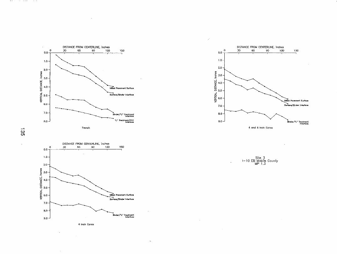
0 0.0
1.0
2.0
" " .s::; 0
.S 3.0
tj
~ 40 en . 0
~ 5.0 1= a: ~
6.0
7.0
B.O
--'-c.u 01
0 0.0
1.0
2.0
" " {j 3.0 .S
~ 4.0 I-' en 05.0
;5 ~ 6.0 ~
7.0
B.O
9.0
DISTANCE FROM CENTERLINE, inches 30 60 90 120 150
Trench
DISTANCE FROM CENTERLINE, inches
Unfed Pavement Surface
Surface/Binder Interface
Binder/'1-" Treatment Interface
"L" Treatment/Pee Interloce
30 60 90 120 150
4 inch Cores
Milled Pavoment Surface -. Surfoee/Blnder Interface
Blnderj'1-.. Treatment Interlace
0 0.0
1.0
2.0
" '" {j 3.0 .S
tj 4.0
~ en 05.0
;5 ~ 6.0
7.0
B.O
9.0
DISTANCE FROM CENTERLINE. inches 30 60 90 120
4 and 6 Inch Cores
Site 3 I-lOEB Mobile County
MP 1.3
150
Milled Pavement Surface
Surlace/Binder Interface
Binder/"L" Treatment Interface
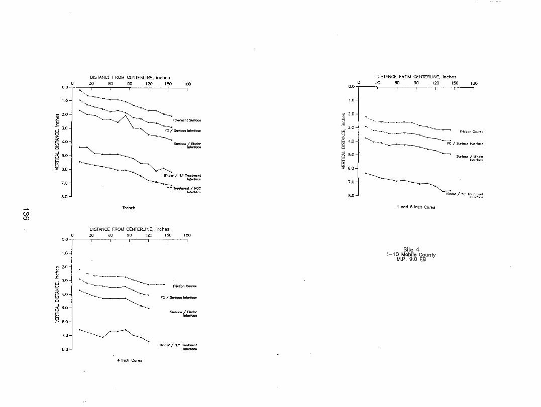
---' tv (J)
0 0.0
1.0
(f) 2.0
'" .<: U c
'-:' 3.0 w u
~ 4.0 VJ (5
~ 5.0
~ ~ 6.0
7.0
8.0
DISTANCE FROM CENTERLINE, inches
~ ~ 00 lW 1~ 100
'"
<==-~ "---'==:~povem.nt Surloce
----.
~ Surlo.lnborloce
Trench
Surface rn=t:~~
Binder / "l." Treatment Interface
'1..." Treatment / pee Interfoce
DISTANCE FROM CENTERLINE, inches o 30 60 90 120 150 180
0.01
1.0 I
1 (f) 2.0-j OJ • .c I U I c: . __ 3.0 w u z ~ VJ (5
4.0
~ 5.0 i= ~
~ 6.0
Fricb"on COUllie ~==-==-=:::-~
Fe / Surface Interface
Surfoce / Binder Interface
7.0-1 ------~ B.O ..J Binder / 1\.11 Treotment
Interface
4 Inch Cores
DISTANCE FROM CENTERLINE, inches
o ~ ~ 00 lW 1~ 100
OO~
~ :: '- -------~ .~- 3.01 " -------------~ ---.--~ .. -----------~ ............ -------~ 4.0. ~-.-___ ~ I Surloce Interlace
~~ -·1-~ Interface Ii:
Friction Cou~e
~ 6.0
7.0
8.0
4 and 6 Inch Cores
Site 4 1-10 Mobile County
M.P. 9.0 EB
Binder / "L" Treatment Interface
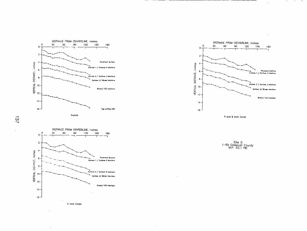
--'-W
'"
'" '" .c u
.S
tf z ~
DISTANCE FROM CENTERLINE. inches o .30 60 90 120 150 180
0,----,,----r----~--~~--~--_2
:~ --~-f----~ ~rlOCei 1 / Surface 2 Interloce
o ' ___________ ~
8 ~ --------~rtoe' 2 / Su,'oe. J Int.rtoco '------.. ~ <t 10 l -~ S'''oco J/ Bind" Int,"oco
~ Binder/ CTS Interlace
1I1 is
W > 12
14
1 6 ...J Tap of F'lflIt CTS
DISTANCE FROM CENTERLINE. inches 0
0 .30 6n 9n PO 150 ,,,n
2
'" 4 ., .c u
.S 6
W U Z ~ 8 If)
Ci
3 10 ;::: 0:: W > 12
I
"J 16
~~~,-~rloce 1 / Surface 2 Interlace ------.---~
~---------- udoe, J Int,rtoco -.--..".----..~urfoce 2 / s
~ ~ JI Binder InterlocfI _ ~ Sudoco
Binder / C'r.) Interlace
Trench 4 and 6 Inch Cares
DISTANCE FROM CENTERLINE. inches 0
0 .30 60 90 120 150 180
2
'" 4 III .c u c ...
6
~ 1-< 8~ If)
Ci
3 10 ;::: 0::
~ 12
~ Pavement Surtace ""-.. ,. Surface 1 / Surface 2 Interloce . ..."
~ ..... -'""--. ~~------------ ISurfoce J Interlace ~ ~rfQCe2
~ ~ J/Blnd"ln""oco - Sunceo
Blnder/ CTS Interlace
14
16
4 Inch Cares
Site 5 1-65 Conecuh County
M.P. 93.1 NB
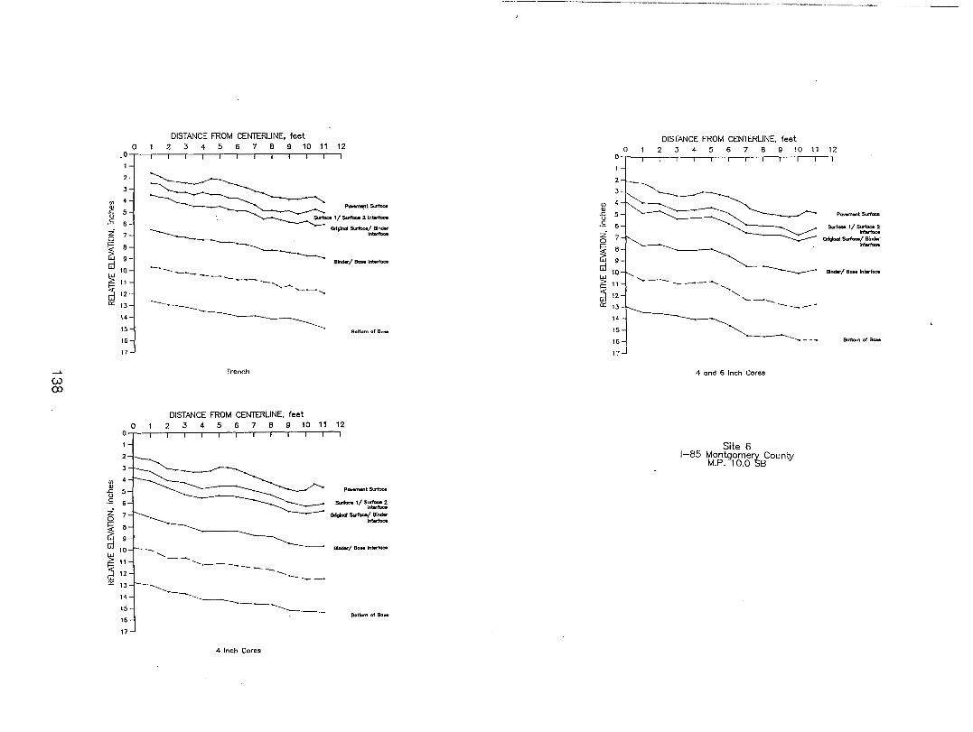
...... W ex>
0
2
3
"' 4 II>
5 .<: u .s Z 7 a ~ 8
GJ G:! 10
~ 11 ...., d 12
a:: 13
"'
14
15
16
17
o
2
3
1! 5 u
.S
Z 7 a ~ 8
GJ cd 10
~11 .... d 12
a:: 13
14
15
16
17
0
DISTANCE FROM CENTERLINE, feet 2 ;3 4 5 6 7 B 9 10 11 12
~ P~Sufoce
........ 1/ ........ 2 Intwfooo
- ~ -'---~ -- -'-.~ ~- ....
_._------------..... ....
Trench
DISTANCE FROM CENTERLINE, feet
"""''''' ........ /81_ In_
mndw/ BOM Int.rlooe
Bottom of BaM
o 2;3 4- 5 6 7 B 9 10 11 12
- '-
~
------------............ -----'------
-------------------------------4 Inch Cores
Pcw.ment Su1oc>a
~ 1/ Slrlooe 2. Intwfooo
Orig!"" ........ /BI_ Intwfooo
BInder / Bo.. Intttfool;
Bottom of BaM
DISTANCE FROM CENTERLINE. feet o ;3 4 5 6 7 B 9 10 11 12
"' II> -U Pavwnont SI.rloca
.£ 6
Z 7 a ~ 8
GJ cd 10
~ 11 ;:::
d 12
a:: 13
14
15
16 .
I,J
~--""'----..... --., '--------
'-------.----
4 and 6 Inch Cores
Site 6 1-85 Montgomery County
M.P. 10.0 S8
su-toc. 1/ Slrlooe 2 In,""","
"""''''' ........ /01_ In,""","
81ndr/ BCIM Intwfootl
Bottom of 80M
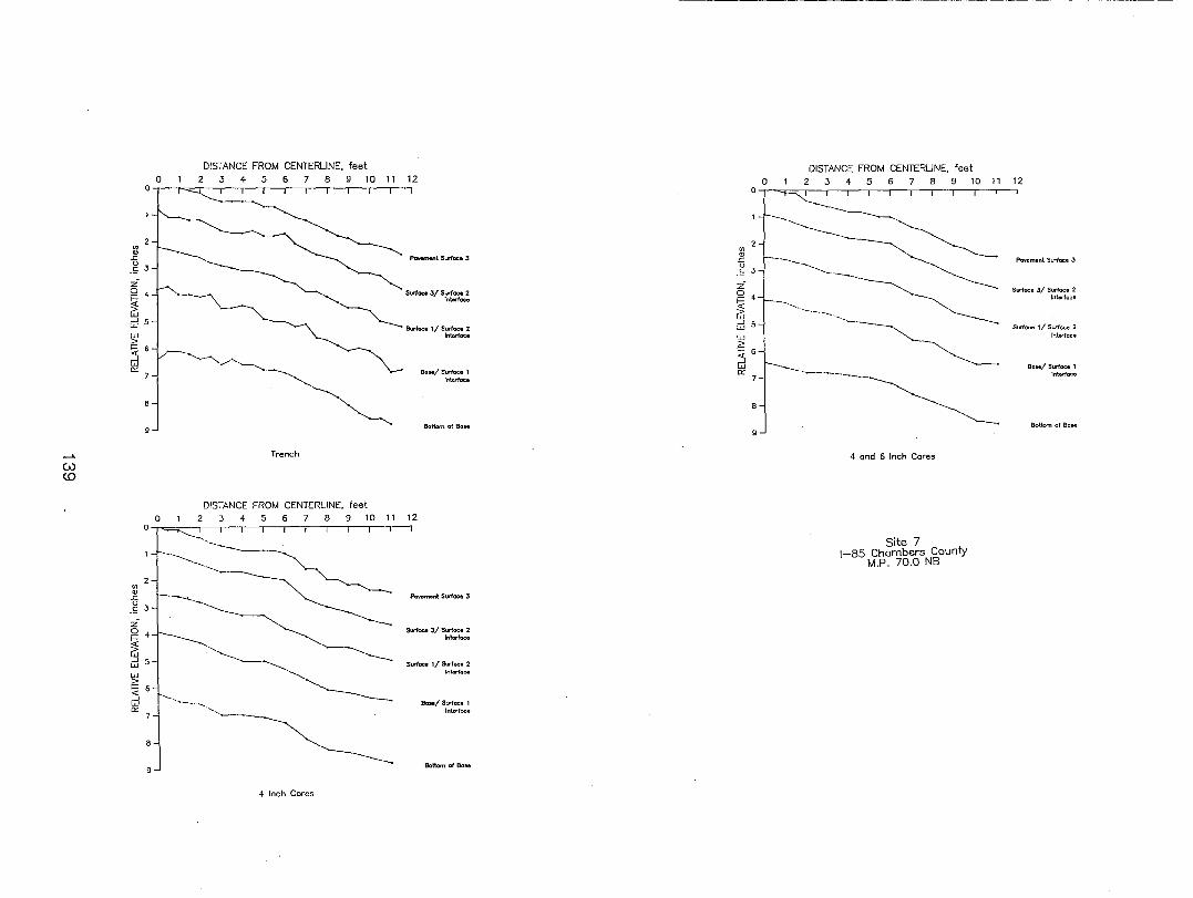
....... W CD
DISTANCE FROM CENTERLINE. feet o 2 3 4 5 6 7 B 9 10 11 12
o I i~
IJJ
'" .<:
.~ J
Z g 4
~ ;:;:I 5
~ ~ W ~
IJJ
'" .<:
o
.~ 3
z o ~ (;j ;:;:I 5
~ ~ 6 w a::
8
' ......
Trench
DISTANCE FROM CENTERLINE. feet
Pavwnent SlIfoce 3
Surfoc.e 3/ SLrfa~ 2 Interfaco
&.rfoctI 1/ Surface 2 Intorfoce
90M/ Surface 1 Interlace
Bottom of BaH
o 2 3 4 5 6 7 B 9 10 11 12 I==:=:;:::::
-'--~ .................
--.....
.'
.' ...... _-"---'-~
4 Inch Cores
.....
Pavement Sl.W"foee J
Surface J/ Slrloce 2 Intoriooo
Surface 1/ Surface 2 Interlo_
BOMI St.r1oce 1 Interlace
Bottom or BaM
DISTANCE FROM CENTERLINE. feet o 2 3 4 5 6 7 B 9 10 11 12
l~~ tS<orlaoo' ----- P ...... on
.' ,_., ~ -----..---~ ---- Surface 3/ IntorlaclI
.~ J
Z ~~ "'_, Q, ~ - -. ~ .. ~-~.~-----~ (;j
;:;:15 ~. w ~ 6
~ ~---~ 8-l
9
4 and 6 Inch Cores
Site 7 \-85 Chambers County
M.P. 70.0 NB
BOM/ Surface 1 lntor1'ac:o
Bottom of BaM
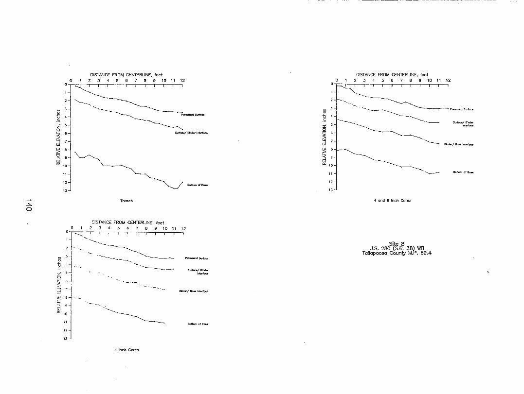
~
~ o
DISTANCE FROM CENTERliNE, feet o 2 3 4 5 6 7 a 9 10 11 12
o
'" 3 i! ~ p-""""" .~~ u .S .-; 5 o ~ 6
~ 7
~ B
;;3 9 a:: 10
11
12
13
s.:rt-/ Elndw 'n~
Botbn of BaM
Trench
DISTANCE FROM CENTERLINE, feet o 2 3 4 5 6 7 agiO 11 12
°r~ I I
~ I -.~--"--.~ (f) 31 ---__ ._ "-----____ Pavement SlIfoco
-5 "J -' ____ c r' ~ ____ ':i 5~ ~ oj ~ ,
"--J • 1 I
W 8-t-
~ I :s 9-1
[1j
~ 10~1 11
12
13
'-----
.. _-----..
'~
4 Inch Cores
Surfoce/ BInder Interloce
Bindet"/ BON Int:Bl"'face
Bottom of B~
DISTANCE FROM CENTERLINE, feet o 1 2 3 4 5 6 7 a 9 10 11 12
~F~' I I I I I I I
? -'--- ---l~-- ~ ~ .} -i "- ______ -~ -~ Povoment Sl¥'faco
~ L -g 4 ~~ .- ---Z 5 o ~ 6
S\rlocej BIndel" ,,_
~ '---- mn_/ BQM Intw1ace
~ B
~ 9 a:: 10
11
12
13
'~-~
4 and 6 Inch Cores
Site 8 U.S. 280 (S.R. 38) W8
Tallapoosa County M.P. 69.4
Bottom of 8QM
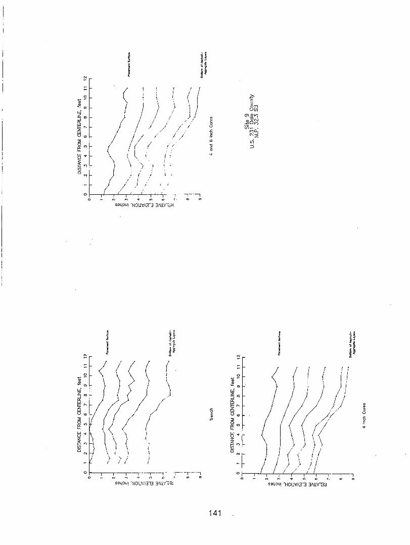
~
:: 0 .... ~
Q) Q)
.... Ol
w 3'" 0::
~r-w U to
::!:
~"' ti"" ~'" Ul 0
N
0
:: o .... ~
Q) Q) -Ol
0
i i j
1 I I I \
) I / ,
/ / / / j I , , / // / I
/
( I (' / / ( , , /
{ l, \ '; J I , I
I
/1 J i J J ,
~-T"---l- .,.-.., .. on "' ,. sa4~U! 'NOUVJ\.iTl 3NlV,:;IJ
1 1 1
I
H !~ 'Ot j~
' ( i ( \ ,
J/ / /
/
-,---, <Xl 0>
" ~ u .r:
" E
'" "0 c 0
'r
r.
" c
" ~
141
-"> c ::J om U(J)
m<Dn <DON -,-,On l7i~
no.: N::;i vi ::)
sa4~U! 'NOIIV,Bl3 3J\ll\fl3C!
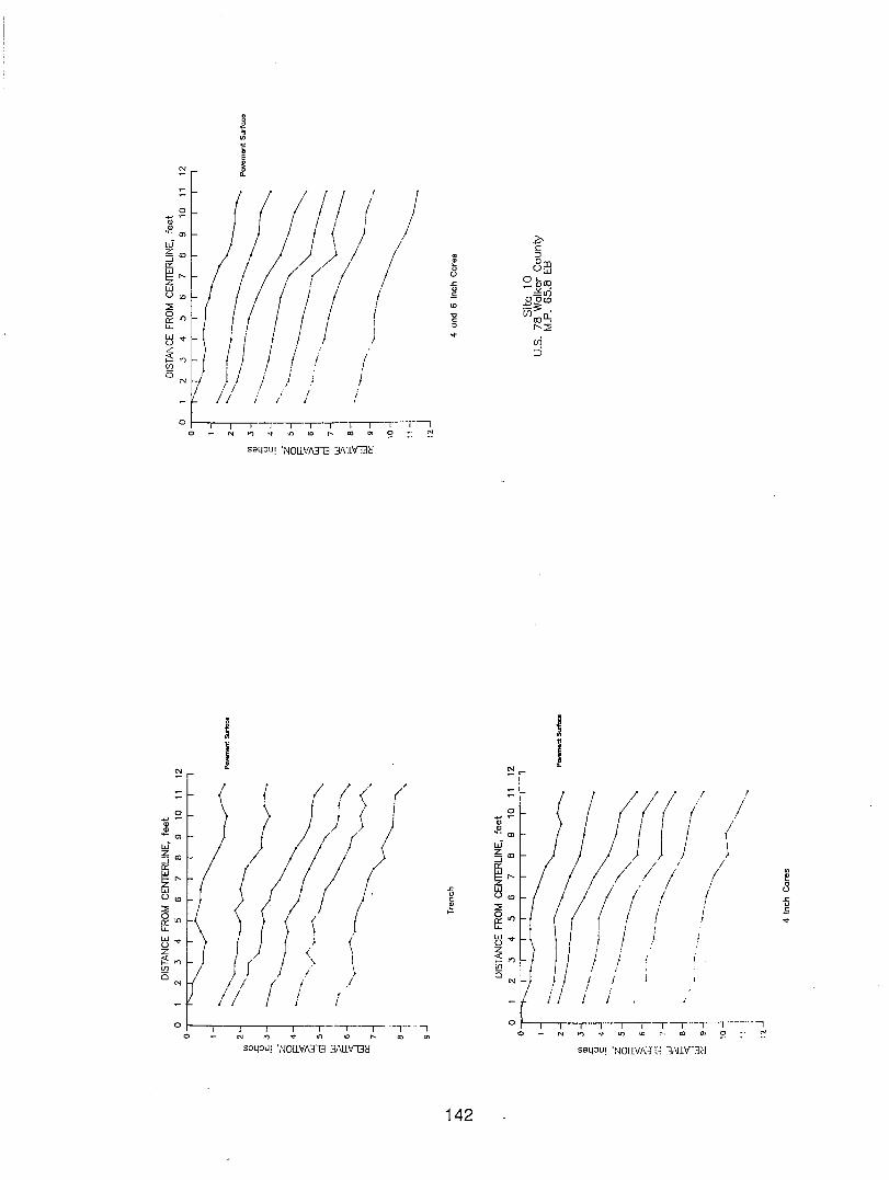
:: .... ~ /11 / / ~: / ) i / I::! " / I (/ /
/ /
/ I
I I !: I I 1/ / I I
g"1 j I) / I / ONj' I J)'
j l/I !
J I J
J i I j J
o ~~~~-'--'--~--r-r--r-I-"-T----'
:: o .... ~
" " ~'" W ~1Xl 0::
~" W U'" ::; ~Il) u.. tj .... Z ~"1 If)
15 N
o _ N ~ ~ ~ w ~ ~ 00 ~ :: ~
,
f ((: ( } r J / )
I / I I / I I I I
I I J i o f---.----r--.---�~..,...I --,---,- -,-- . .,
o ~ ~ ~ ~ ~
sa4:lu! 'NOll'v'lI3l3 3J\uV13t1
'" e o u .s:;
~
'" '0 c: o ....
.r. u c:
~
142
/ ,I I !
( (( (
/ ) J / I / .I /
/ ' I
j ( ( I /
, I j ) I ' Ii,
} i f / / 1
J/ ! i
i J
/ f
/
I
o I'---r--~"----,---,--,--, -,- ----,---", --1" ' " o - N ~ ~ ~ ~ ~. ~ mO·" ~
Sa4:lU! 't~OI.lVJ\n'J ::J,\i.lVBiJ
'" 8 .s:; u .E ....
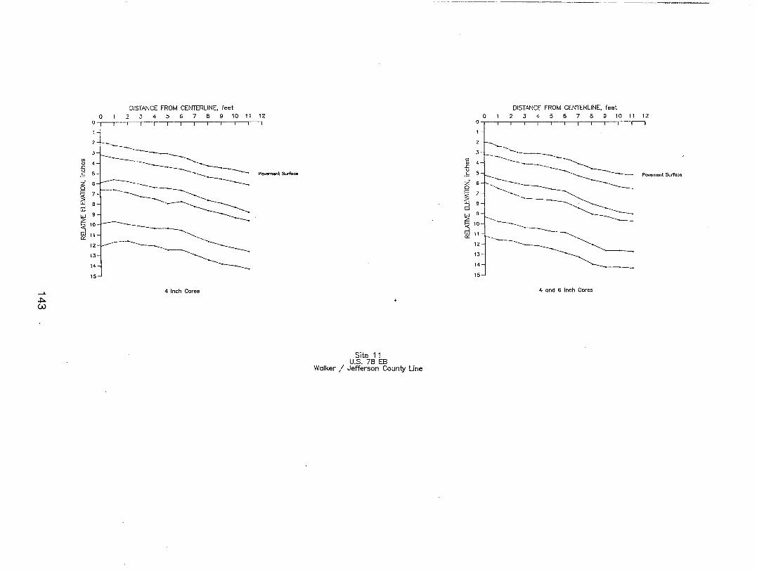
...... +:>w
DISTANCE FROM CENTERLINE. feet ? 3 4 5 01_ 9 10 11 678
o 1""""'-,---- I • ...j
'1-
, -===--=~--------==== ~ 4 ..c:: g 5
.- ----------------.. g 6 __________ ~------------------F 7 ___ ,__ ~
~ B
G:! 9
~ 10 ___ ~ __ __________
~" ~-------------------12 _____ _____. 13
14
15
4 Inch Cores
12
Pavomont Surface
Site 11 U.S. 78 EB
Walker / Jefferson Coun1;y Line
DIST."NCE FROM CENTERLINE. feet 0 2 3 4 5 6 7 8 9 10 11 12
0 .,-----,,---.--,---.1 -----,------r-- -- I
2
3 en
4 Q) ..c::
" 5 .!:
Z 0
~ 7
G:i B -' w gJ ~ ~ 10
0:: 11
12
13
14
-------------_~ ________ ~ Pavement Surface
~- ---~ _.--------- -------~~~
"--15
4 and 6 Inch Cores
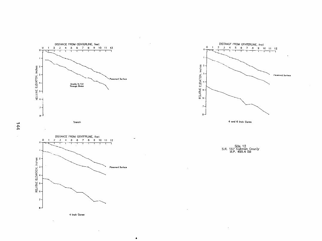
-L
~ ~
DISTANCE FROM CENTERLINE. feet o 2 3 4 5 6 7 8 9 10 11 12
o • I
en ~ u
,<: z:3 o ~ ~ 4
d W 5 ;?: ::r. ~ Ij~
:j
~~
~'-'~ Pavoment Surlaee
Unable toa" ~'! Through In
Trench
DISTANCE FROM CENTERLINE. feet o 2 3 4 5 6 7 8 9 10 11 12
:~ :(l 2 .c u
,<: _ 3
Z o 1=
~ 4
d ~ 5
~ <r 6
7
a
----
"
"--"
4 Inch Core.
Pavement Surface
•
DiSTANCE FROM CENTERLINE. feet o 1 2 3 4 5 6 7 8 9 10 11 12
:r~~" -.....---.. --, en 2 ",
~ I '----~ i 3 ~ Pavement Suriae.
~ 4~ d ~ 5
~ <r 6
a ~ 4 and 6 Inch Cores
Site 12 SR, 157 Cullman Couni;y
M.P, 495-.4 S8
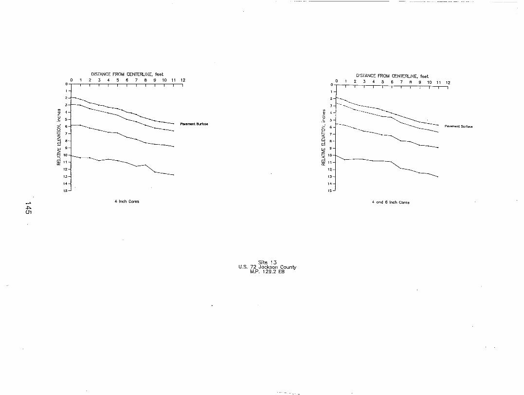
-'-.J:>. 01
o o I
3
:g 4 -<:
.~ 5
Z 6 o ~ 7
~ B
~ 10
tt!11 12
13
14
15
DISTANCE FROM CENTERLINE. feet 2 3 4 5 6 7 8 9 10 11 12
Pavement Surface
4 Inch Cores
Site 13 U.S. 72 Jackson County
M.P. 129.2 EB
"' Q) -<: u c
DISTANCE FROM CENTERLINE. feet
; 6f--""""""" ------- ~ Pavement Surface ~ 7 -.-~-----GJ B G:l Ij; 9
~ 10
a::: 11
12
13
14
15
4 and 6 Inch Cores
Recommended