Embed Size (px)
Citation preview

WL | delft hydraulics
Description of TRANSPOR2004 and Implementation in Delft3D-ONLINE
FINAL REPORT
November 2004
Z3748.00
Report
DG Rijkswaterstaat, Rijksinstituut voor Kust en Zee | RIKZ
Prepared for:

Prepared for:
DG Rijkswaterstaat, Rijksinstituut voor Kust en Zee | RIKZ FINAL REPORT L.C. van Rijn, D.J.R. Walstra and M. van Ormondt
Report Z3748.10
Description of TRANSPOR2004 and Implementation in Delft3D-ONLINE
WL | delft hydraulics CLIENT:
DG Rijkswaterstaat Rijks-Instituut voor Kust en Zee | RIKZ
TITLE:
Description of TRANSPOR2004 and Implementation in Delft3D-ONLINE, FINAL REPORT
ABSTRACT: In 2003 much effort has been spent in the improvement of the DELFT3D-ONLINE model based on the engineering sand transport formulations of the TRANSPOR2000 model (TR2000). This work has been described in Delft Hydraulics Report Z3624 by Van Rijn and Walstra (2003). However, the engineering sand transport model TR2000 has recently been updated into the TR2004 model within the EU-SANDPIT project. The most important improvements involve the refinement of the predictors for the bed roughness and the suspended sediment size. Up to now these parameters had to be specified by the user of the models. As a consequence of the use of predictors for bed roughness and suspended sediment size, it was necessary to recalibrate the reference concentration of the suspended sediment concentration profile. The formulations (including the newly derived formulations of TR2004) implemented in this 3D-model are described in detail. The implementation of TR2004 in Delft3D-ONLINE is part of an update of Delft3D which involves among others: the extension of the model to be run in profile mode, the synchronisation of the roughness formulations and inclusion of two breaker delay concepts. The present report describes the implementation of TR2004 formulations in Delft3D-ONLINE in detail.
REFERENCES:
Overeenkomst RKZ-1392
VER. ORIGINATOR DATE REMARKS REVIEW APPROVED BY 1 Walstra 18 May 2004 Draft Van Rijn van der Weck2 Walstra 28 May 2004 Interim Van Rijn van der Weck3 Walstra 11 November 2004 Final Van Rijn Schilperoort PROJECT IDENTIFICATION: Z3748
KEYWORDS: TRANSPOR2004, Delft3D, Breaker Delay
NUMBER OF PAGES 78
CONFIDENTIAL: YES, until (date) NO
STATUS: PRELIMINARY DRAFT FINAL

Description of TRANDPOR2004 and Implementation in Delft3D-ONLINE Z3748.10 November, 2004 FINAL REPORT
WL | Delft Hydraulics i
Contents
1 Introduction ................................................................................................... 1—1 2 UPDATED TRANSPOR2004-MODEL ...................................................... 2—1
2.1 Introduction.........................................................................................................2—1
2.2 Updated sand transport model TRANSPOR2004 (TR2004) ..........................2—1
2.2.1 Bed roughness predictor ..........................................................................2—1
2.2.2 Predictor for suspended sediment size.....................................................2—4
2.2.3 Thickness of wave-boundary layer, fluid mixing and sediment mixing layer .........................................................................................................2—4
2.2.4 Wave-induced bed-shear stress ................................................................2—5
2.2.5 Wave-induced streaming..........................................................................2—6
2.2.6 Shields criterion for initiation of motion .................................................2—6
2.2.7 Bed-load transport ...................................................................................2—7
2.2.8 Wave-related suspended transport ...........................................................2—8
2.2.9 Near-bed sediment mixing coefficient .....................................................2—8
2.2.10 Reference concentration and reference level ...........................................2—8
2.2.11 Recalibration............................................................................................2—9
2.3 Intercomparison of transport rates based on TR2004 with TR2000 and TR1993...............................................................................................................2—15
2.4 Application of TR2004-model for graded sediment.......................................2—17
2.4.1 Experiments ...........................................................................................2—17
2.4.2 Model results .........................................................................................2—20
3 Sand transport formulations in DELFT3D model ..................................... 3—1
3.1 Introduction.........................................................................................................3—1
3.2 Model description ...............................................................................................3—2
3.2.1 Hydrodynamics........................................................................................3—2

Description of TRANDPOR2004 and Implementation in Delft3D-ONLINE Z3748.10 November, 2004 FINAL REPORT
WL | Delft Hydraulics i i
3.2.2 Waves.......................................................................................................3—8
3.2.3 Sediment dynamics and bed level evolution............................................3—9
3.2.4 Erosion and deposition...........................................................................3—20
3.2.5 Wave-related suspended transport .........................................................3—24
3.2.6 Bed load transport..................................................................................3—26
3.2.7 Transport Calibration Factors ................................................................3—27
3.3 Implementation Check of TR2004 in Delft3D................................................3—28
3.4 Miscellaneous Improvements to Delft3D ........................................................3—28
4 Conclusions .................................................................................................... 4—1 5 References ...................................................................................................... 5—1
Description of TRANDPOR2004 and Implementation in Delft3D-ONLINE Z3748.10 November, 2004 FINAL REPORT
WL | Delft Hydraulics 1 — 1
1 Introduction
RIKZ of Rijkswaterstaat and Delft Hydraulics are working together on the development/improvement, verification/validation and evaluation of morphodynamic models within the framework K2005 of Rijkswaterstaat (see Report Z2478 of Delft Hydraulics and Website http://vop.wldelft.nl) and within the SANDPIT-project (website: http://sandpit.wldelft.nl). In 2003 much effort has been spent in the improvement of the DELFT3D-ONLINE model based on the engineering sand transport formulations of the TRANSPOR2000 model (TR2000). This work has been described in Delft Hydraulics Report Z3624 by Van Rijn and Walstra (2003). However, the engineering sand transport model TR2000 has recently been updated into the TR2004 model within the EU-SANDPIT project. The most important improvements involve the refinement of the predictors for the bed roughness and the suspended sediment size. Up to now these parameters had to be specified by the user of the models. As a consequence of the use of predictors for bed roughness and suspended sediment size, it was necessary to recalibrate the reference concentration of the suspended sediment concentration profile. Given the updated TR2004 model, an effort was necessary to further improve the DELFT3D-ONLINE model using the formulations of the updated TR2004 sand transport model (see Chapter 2). This latter work has been reported in Chapter 3. Chapter 2 addresses the description of the updated TR2004 model and the recalibration of the reference concentration using field and laboratory data sets. Furthermore, the results of the TR2004 model have been compared with results from older versions (TR1993 and TR2000) of the sand transport model Chapter 3 addresses the central focus point of the study: the DELFT3D-ONLINE model. The formulations (including the newly derived formulations of TR2004) implemented in this 3D-model are described in detail. The implementation of TR2004 in Delft3D-ONLINE is part of an update of Delft3D which involves among others: the extension of the model to be run in profile mode, the synchronisation of the roughness formulations and inclusion of two breaker delay concepts. The present report describes the implementation of TR2004 formulations in Delft3D-ONLINE in detail. Some general conclusions are given in Chapter 4.

Description of TRANDPOR2004 and Implementation in Delft3D-ONLINE Z3748.10 November, 2004 FINAL REPORT
WL | Delft Hydraulics 2 — 1
2 UPDATED TRANSPOR2004-MODEL
2.1 Introduction
A new version of the TRANSPOR model has been made (TR2004) based on the results of former studies, particularly those of 2003 (Van Rijn and Walstra, 2003). The basic formulations of the TR1993-model are described in Appendix A of Van Rijn (1993). Detailed information on the Multi-fraction method can be found in Van Rijn (2000). The modifications concern the following points: • Predictor of bed roughness; • Predictor of suspended sediment size • Grain roughness and friction factor; • Wave-induced orbital velocities and streaming near the bed; • Wave-induced bed-shear stress; • Wave-induced sand transport; • Shields criterion for fine sand; • Bed load transport model • Mixing near the bed; • Reference concentration. In 2003 new bed roughness predictors to simulate the effective roughness of various types of bed forms were developed and implemented in the latest version of the TRANSPOR-model and in the DELFT3D-model. Experiences so far showed an unrealistic behaviour of the roughness predictors of mega-ripples and dunes. Therefore, the predictors of mega-ripple roughness and dune roughness were adjusted slightly resulting in the updated TR2004-model. The roughness predictor of small-scale ripples in current, waves and combined current-wave conditions was not changed. In line with this, the predictor of the suspended sediment size was slightly modified.
2.2 Updated sand transport model TRANSPOR2004 (TR2004)
2.2.1 Bed roughness predictor
The TR2004 model includes a bed-roughness predictor for the current-related and wave-related bed roughness parameters. In TR1993 and TR2000 both parameters have to be specified as user-related input data. Physical current-related bed roughness It is assumed that the physical bed roughness of movable small-scale ripples in natural conditions is approximately equal to the ripple height: ks,c≅∆ r. Furthermore, it is assumed that the small-scale ripples are fully developed with a height equal to ∆r=150d50 for ψ≤50 in

Description of TRANDPOR2004 and Implementation in Delft3D-ONLINE Z3748.10 November, 2004 FINAL REPORT
WL | Delft Hydraulics 2 — 2
the lower wave-current regime and that the ripples disappear with ∆r=0 for ψ≥250 in the upper wave-current regime (sheet flow conditions). The expressions implemented for small-scale ripples are given by:
( ), , 50
, , 50
, , 50
150 0 50 ( , )
182.5 0.65 50 250 ( , )
20 250 ( )
s c r
s c r
s c r
k d and lower wave current regime SWR ripples
k d and upper wave current regime sheet flow
k d and linear approach in transitional regime
ψ
ψ ψ
ψ
= ≤ ≤ −
= − < < −
= ≥
(2.2.1)
with: ψ= mobility parameter=Uwc
2/((s-1)gd50)), (Uwc)2= (Uδ,r)2+ vR 2
Uδ,r= representative peak orbital velocity near bed based on the method of Isobe-Horikawa, see Equation (2.2.16), vR = depth-averaged current velocity, ϕ= angle between wave and current motion, Hs= significant wave height, k=2π/L, L= wave length derived from (L/Tp± vR)2=gL tanh(2πh/L)/(2π), Tr= Tp/((1-( vRTp/L)cosϕ)= relative wave period, Tp= peak wave period, h= water depth.
Equation (2.2.1) is assumed to be valid for relatively fine sand with d50 in the range of 0.1 to 0.5 mm. An estimate of the bed roughness for coarse particles (d50>0.5 mm) can be obtained by using Equation (2.2.1) for d50=0.5 mm. Thus, d50=0.5 mm for d50≥0.5 mm resulting in a maximum bed roughness height of 0.075 m (upper limit). The lower limit will be ks,c,r=20d50= 0.002 m for sand with d50≤0.1 mm. When mega-ripples and/or dunes are present on the seabed (if h=water depth>1 m and vr=depth-averaged velocity>0.3 m/s), the physical form roughness (ks,c,mr) of the mega-ripples and dunes should also be taken into account (grain roughness is negligibly small; only form roughness). Compared with the bed roughness predictor implemented earlier (Van Rijn and Walstra, 2003), the expressions of the current-related bed roughness due to mega-ripples and dunes have been refined into: Mega ripples:
( ), ,
, ,
, ,
, ,
0.0002 0 50 1
0.011 0.00002 50 550 10 550 1
0.02 0.2
s c mr
s c mr
s c mr
s c mr
k h and and h
k h and and hk and and h
k
ψ ψψ ψ
ψ
= ≤ ≤ >
= − < < >= ≥ >
≤ ≤
(2.2.2)
Dunes (only applicable in rivers, .i.e. no waves):
( ), ,
, ,
, ,
, ,
0.0004 0 100 1
0.048 0.00008 100 600 10 600 1
0.02 1.0
s c d
s c d
s c d
s c d
k h and and h
k h and and hk and and h
k
ψ ψψ ψ
ψ
= ≤ ≤ >
= − < < >= ≥ >
≤ ≤
(2.2.3)
Equation (2.2.2) yields: ks,c,mr=0.01h for ψ=50 and ks,c,mr=0 for ψ=550. Hence, the maximum value is ks,c,mr=0.01h. The absolute maximum value of the mega-ripple roughness is assumed to be 0.2 m

Description of TRANDPOR2004 and Implementation in Delft3D-ONLINE Z3748.10 November, 2004 FINAL REPORT
WL | Delft Hydraulics 2 — 3
Equation (2.2.3) yields: ks,c,d=0 for ψ=0, ks,c,d=0.04h for ψ=100 and ks,c,d=0 for ψ=600. Hence, the maximum value is ks,c,d=0.04 h. The absolute maximum value of the dune roughness is assumed to be 1.0 m. It is remarked that Equations (2.2.2) and (2.2.3) are slightly different from those presented in 2003 (see Equations 3.1.10 and 3.1.11 of Van Rijn and Walstra, 2003), because these latter expressions showed a less realistic behaviour at larger bed-shear stresses. When mega-ripples and/or dunes are present, these values are added to the physical current-related bed roughness of the small-scale ripples by quadratic summation, as follows:
( )0.52 2 2, , , , , , ,s c s c r s c mr s c dk k k k= + + (2.2.4)
The current-related friction coefficient (based on the Darcy-Weisbach approach: f=8g/C2) can be computed as:
2 2
, ,
8 0.24
12 1218log logc
s c s c
gfh h
k k
= =
(2.2.5)
During the Sandpit-project, bed roughness values in the range of 0.05 to 0.25 m have been observed at the Noordwijk site (water depth = 12 m, D50 = 0.2 mm, current = 0.1 to 0.5 m/s, Hs = 0 to 3 m. Equation (2.2.4) yields values in the range of 0.05 to 0.15 m for the Noordwijk site. Physical wave-related roughness of movable bed ks,w As regards the physical wave-related bed roughness, only bed forms (ripples) with a length scale of the order of the wave orbital diameter near the bed are relevant. Bed forms (mega-ripples, ridges, sand waves) with a length scale much larger than the orbital diameter do not contribute to the wave-related roughness. The physical wave-related roughness of small-scale ripples is given by:
( )
, , 50
, , 50
, , 50
150 50(lower wave-current regime, SWR ripples)20 250(upper wave-current regime, sheet flow)
182.5 0.65 50 250(linear approach in transitional regime)
s w r
s w r
s w r
k d fork d for
k d for
ψψ
ψ ψ
= ≤= ≥
= − < <
(2.2.6)
with: ψ= mobility parameter=Uwc
2/((s-1)gd50)), (Uwc)2= (Uδ,r)2+ vR 2, Uδ,r= representative
peak orbital velocity near bed based on the method of Isobe-Horikawa, see Equation (2.2.16), vR = depth-averaged current velocity, ϕ= angle between wave and current motion, Hs= significant wave height, k=2π/L, L= wave length derived from (L/Tp± vR)2=gL tanh(2πh/L)/(2π), Tr= Tp/((1-( vRTp/L)cosϕ)= relative wave period, Tp= peak wave period, h= water depth.
Equation (2.2.6) includes grain roughness and is assumed to be valid for relatively fine sand with d50 in the range of 0.1 to 0.5 mm.

Description of TRANDPOR2004 and Implementation in Delft3D-ONLINE Z3748.10 November, 2004 FINAL REPORT
WL | Delft Hydraulics 2 — 4
The wave-related friction coefficient is computed as:
0.19
, ,
exp 5.2 6ws w r
Afk
δ
− = −
(2.2.7)
Apparent bed roughness for flow over a movable bed It is proposed to use the existing expression:
,' ', ,
exp 10ra a
s c R s c MAX
Uk kandk v k
δγ = =
(2.2.8)
with: Uδ,r= representative peak orbital velocity near the bed (see Equation (2.2.16)), vR= depth-averaged current velocity, γ=0.8+ϕ-0.3ϕ2, ϕ= angle between wave direction and current direction (in radians between 0 and π; 0.5π= 90o, π= 180o) and '
,s ck is the current-
related bed roughness excluding dunes. Characteristic γ-values are γ=0.8 for 0, γ=1 for π= 180o and γ=1.63 for 0.5π= 90o. The γ-value is maximum γ=1.63 for ϕ= 0.5π= 90o. Equation (2.2.8) should only be applied to the bed roughness of the small-scale ripples and mega-ripples. The current-related apparent friction coefficient (based on the Darcy-Weisbach approach: f=8g/C) can be computed as:
, 2 28 0.24
12 1218log logc a
a a
gfh h
k k
= =
(2.2.9)
2.2.2 Predictor for suspended sediment size
Compared with the suspended sediment size predictor implemented earlier (Van Rijn and Walstra, 2003), this latter predictor has been refined into:
( )5010, 50
10
50
max 1 0.0006 1 550 550
550
s
s
dd d d ford
d d for
ψ ψ
ψ
= + − − < = ≥
(2.2.10)
2.2.3 Thickness of wave-boundary layer, fluid mixing and sediment mixing layer
In TR2004 the wave boundary layer thickness according to (Davies and Villaret, 1999) is used:

Description of TRANDPOR2004 and Implementation in Delft3D-ONLINE Z3748.10 November, 2004 FINAL REPORT
WL | Delft Hydraulics 2 — 5
0.25
, ,
0.36ws w r
AAk
δδδ
−
=
(2.2.11)
Aδ= peak orbital excursion at edge of wave boundary layer Which replaces the wave boundary layer thickness formulation based on that of Jonsson and Carlsen (1976) used in TR1993 and TR2000. The thickness of the effective fluid mixing layer in TR2004 is modelled as (in metres):
, ,2 0.05 0.2m w m MIN m MAXwith andδ δ δ δ= = = (2.2.12)
The thickness of the effective sediment mixing layer in TR2004 is modelled as:
( )( )min 0.5, max 0.05, 2s br wδ γ δ= (2.2.13)
with:
0.5
1 0.4 1 0.4s sbr br
H Hand forh h
γ γ = + − = ≤
(2.2.14)
2.2.4 Wave-induced bed-shear stress
The time-averaged bed-shear stress is computed as:
( )2, ,
14b w w w rf Uδτ ρ= (2.2.15)
with: ρ = fluid density fw = wave-related friction factor, Eq. (2.2.7) In TR2004 the peak orbital velocity is refined into:
( ) ( )( )1
3 3 3, , ,0.5 0.5r for backU U Uδ δ δ= + (2.2.16)
Uδ,r = representative peak orbital velocity near the bed Uδ,for = peak orbital velocity in forward direction (method of Isobe and Horikawa) Uδ,back= peak orbital velocity in backward direction (method of Isobe and Horikawa) In TR1993 and TR2000 the Uδ,r-parameter was based on linear wave theory.
Description of TRANDPOR2004 and Implementation in Delft3D-ONLINE Z3748.10 November, 2004 FINAL REPORT
WL | Delft Hydraulics 2 — 6
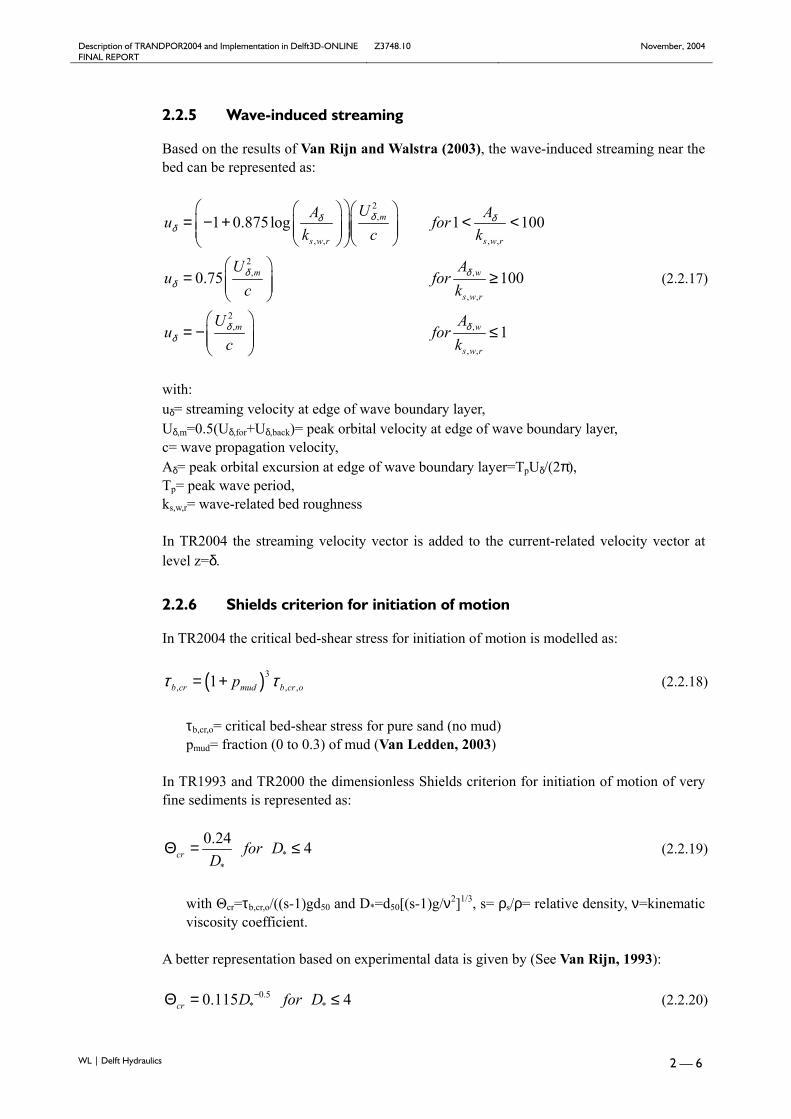
2.2.5 Wave-induced streaming
Based on the results of Van Rijn and Walstra (2003), the wave-induced streaming near the bed can be represented as:
2,
, , , ,
2, ,
, ,
2, ,
, ,
1 0.875log 1 100
0.75 100
1
m
s w r s w r
m w
s w r
m w
s w r
UA Au fork c k
U Au for
c k
U Au for
c k
δδ δδ
δ δδ
δ δδ
= − + < <
= ≥
= − ≤
(2.2.17)
with: uδ= streaming velocity at edge of wave boundary layer, Uδ,m=0.5(Uδ,for+Uδ,back)= peak orbital velocity at edge of wave boundary layer, c= wave propagation velocity, Aδ= peak orbital excursion at edge of wave boundary layer=TpUδ/(2π), Tp= peak wave period, ks,w,r= wave-related bed roughness In TR2004 the streaming velocity vector is added to the current-related velocity vector at level z=δ.
2.2.6 Shields criterion for initiation of motion
In TR2004 the critical bed-shear stress for initiation of motion is modelled as:
( )3, , ,1b cr mud b cr opτ τ= + (2.2.18)
τb,cr,o= critical bed-shear stress for pure sand (no mud) pmud= fraction (0 to 0.3) of mud (Van Ledden, 2003) In TR1993 and TR2000 the dimensionless Shields criterion for initiation of motion of very fine sediments is represented as:
**
0.24 4cr for DD
Θ = ≤ (2.2.19)
with Θcr=τb,cr,o/((s-1)gd50 and D*=d50[(s-1)g/ν2]1/3, s= ρs/ρ= relative density, ν=kinematic viscosity coefficient.
A better representation based on experimental data is given by (See Van Rijn, 1993):
0.5* *0.115 4cr D for D−Θ = ≤ (2.2.20)

Description of TRANDPOR2004 and Implementation in Delft3D-ONLINE Z3748.10 November, 2004 FINAL REPORT
WL | Delft Hydraulics 2 — 7
which is implemented in TR2004.
2.2.7 Bed-load transport
Bed load transport model The net bed-load transport rate in conditions with uniform bed material is obtained by time-averaging (over the wave period T) of the instantaneous transport rate using the bed-load transport model (quasi-steady approach), as follows:
,1
b b tq q dtT = ∫ (2.2.21)
with qb,t = F(instantaneous hydrodynamic and sediment transport parameters). The formula applied, reads as:
( )0.5 '', , ,, ,0.3
, 50 *,
max 0,0.5 b cw t b crb cw t
b t sb cr
q d Dτ ττ
ρρ τ
− − =
(2.2.22)
in which: τ/b,cw,t = instantaneous grain-related bed-shear stress due to both current and wave motion =
0.5 ρ f/cw (Uδ,cw,t)2,
Uδ,cw,t = instantaneous velocity due to current and wave motion at reference height a, see Equation (2.2.8),
f/c = current-related grain friction coefficient =0.24(log(12h/ks,grain))-2,
f/w = wave-related grain friction coefficient=Exp[-6+5.2(Aδ/ks,grain)-0.19],
α = coefficient related to relative strength of wave and current motion: ˆ
ˆR
UU v
δ
δ
α =+
,
Uδ = the peak orbital velocity, vR is the equivalent current velocity calculated at reference height a,
βf = coefficient related to vertical structure of velocity profile, Aδ = peak orbital excursion, τb,cr = critical bed-shear stress according to Shields, ρs = sediment density, ρ = fluid density, d50 = particle size, D* = dimensionless particle size. The two most influential parameters of Eq. (2.2.22) are: '
cwf and ks,grain. Various field data sets from the literature and new data sets (laboratory and field) collected within the SANDPIT project have been used to verify/improve these parameters of the bed-load transport formulations (see Van Rijn and Walstra, 2003).

Description of TRANDPOR2004 and Implementation in Delft3D-ONLINE Z3748.10 November, 2004 FINAL REPORT
WL | Delft Hydraulics 2 — 8
In TR2000, these two parameters ( 'cwf and ks,grain) are modelled as:
( )' ' '1cw f c wf f fαβ α= + − (2.2.23)
, 90 1 3s grain grain graink d with between andα α= (2.2.24)
Based on the findings of Van Rijn and Walstra (2003), the following expressions have been implemented in TR2004:
( )' 0.5 ' 0.5 '1cw f c wf f fα β α= + − (2.2.25)
, 90s graink d= (2.2.26)
2.2.8 Wave-related suspended transport
The wave-related suspended transport component is modelled as follows:
4 4, ,
, 3 3, ,
for backs w
for back
U Uq u cdz
U Uδ δ
δδ δ
γ −
= + + ∫ (2.2.27)
with: Uδ,for= near-bed peak orbital velocity in onshore direction (in wave direction) and
Uδ,back= near-bed peak orbital velocity in offshore direction (against wave direction), uδ= wave-induced streaming velocity near the bed, c= time-averaged concentration and γ= phase lag function.
In TR2004 (based on the findings of Van Rijn and Walstra, 2003), the phase lag function is: γ= 0.1 in stead of γ= 0.2 as was used in TR2000.
2.2.9 Near-bed sediment mixing coefficient
The mixing coefficient near the bed is modelled as:
, ,0.018w bed w s rUδε β δ= (2.2.28)
with Uδ,r according to Equation (2.2.16) and δs according to Equation (2.2.13).
2.2.10 Reference concentration and reference level
The reference level in TR2004 is described by:
( )( ), , , ,min 0.2 ,max 0.5 ,0.5 ,0.01s c r s w ra h k k= (2.2.29)
with h= the local water depth, ks,c,r= current-related bed roughness height due to small-scale ripples and ks,w,r= wave-related bed roughness height due to small-scale ripples.
Description of TRANDPOR2004 and Implementation in Delft3D-ONLINE Z3748.10 November, 2004 FINAL REPORT
WL | Delft Hydraulics 2 — 9
Similarly as in TR1993 and TR2000, the reference concentration (single fraction approach) in TR2004 is described by:
( )( )
1.5
50s ,0.3 0.015 0.05a
a a MAX s
d Tc with c
a Dρ ρ
∗
= = (2.2.30)
2.2.11 Recalibration
The T-parameter of Equation (2.2.30) involves the computation of the wave-related bed-shear stress and a wave-related efficiency factor µw. This latter parameter has been recalibrated using a dataset of 53 cases (see Table 3.2.1) from combined quasi-steady and oscillatory flow cases, resulting in:
( )
*( )
, *
( ), *
0.7
0.35 2
0.14 5
w
w MAX
w MIN
D
for D
for D
µ
µ
µ
=
= <
= >
(2.2.31)
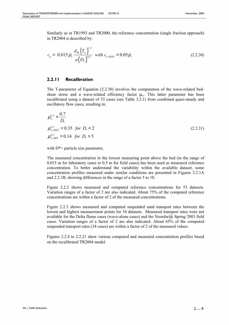
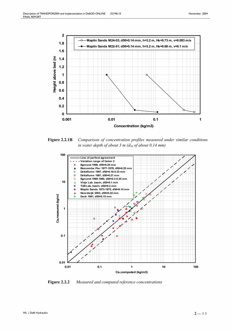
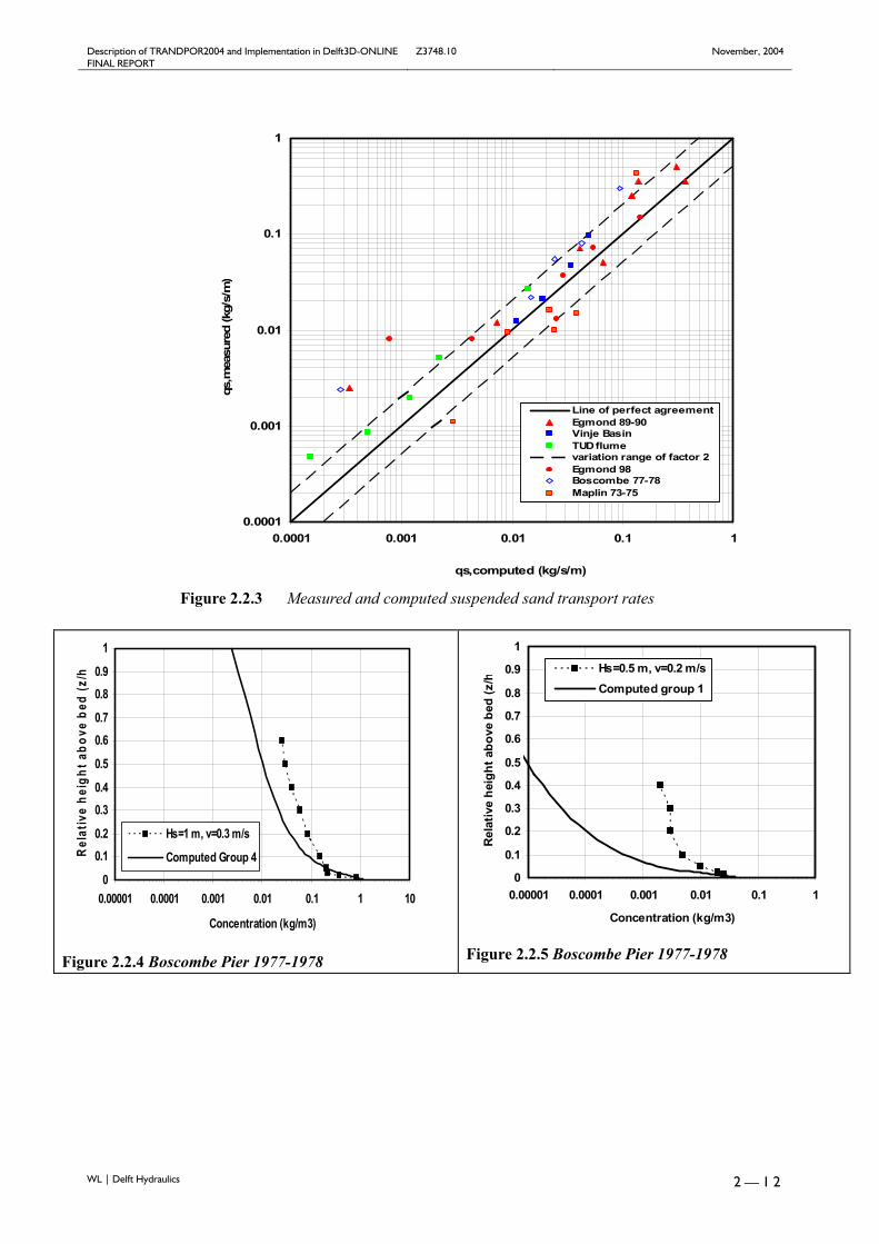
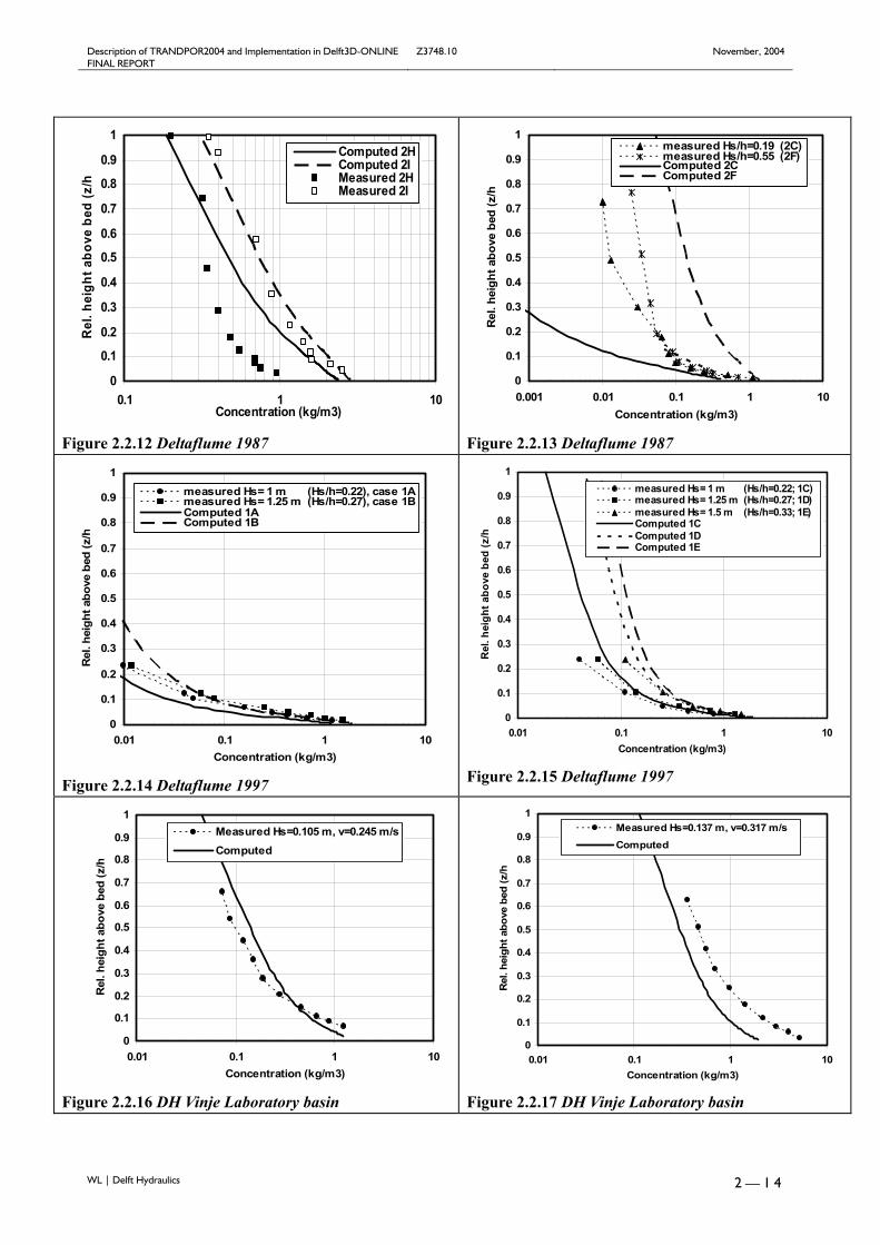
with D*= particle size parameter, The measured concentration in the lowest measuring point above the bed (in the range of 0.015 m for laboratory cases to 0.5 m for field cases) has been used as measured reference concentration. To better understand the variability within the available dataset, some concentration profiles measured under similar conditions are presented in Figures 2.2.1A and 2.2.1B, showing differences in the range of a factor 5 to 10. Figure 2.2.2 shows measured and computed reference concentrations for 53 datasets. Variation ranges of a factor of 2 are also indicated. About 75% of the computed reference concentrations are within a factor of 2 of the measured concentrations. Figure 2.2.3 shows measured and computed suspended sand transport rates between the lowest and highest measurement points for 34 datasets. Measured transport rates were not available for the Delta flume cases (wave-alone cases) and the Noordwijk Spring 2003 field cases. Variation ranges of a factor of 2 are also indicated. About 65% of the computed suspended transport rates (34 cases) are within a factor of 2 of the measured values. Figures 2.2.4 to 2.2.21 show various computed and measured concentration profiles based on the recalibrated TR2004 model.

Description of TRANDPOR2004 and Implementation in Delft3D-ONLINE Z3748.10 November, 2004 FINAL REPORT
WL | Delft Hydraulics 2 — 1 0
Site Sediment
size d50 (mm)
Water depth range (m)
Wave height range (m)
Flow velocity range (m/s)
Reference
Boscombe 1977-1978
0.25 4.8-5.3 0.45-1.05 0.2-0.4 Whitehouse et al., 1997
Maplin sands 1973-1975
0.14 2.8-3.2 0.4-0.9 0.07-0.34 Whitehouse et al., 1996
Egmond 1989-1990
0.3-0.35 1-1.6 0.2-0.9 0.06-0.55 Kroon, 1994 Wolf, 1997
Egmond 1998 0.25 2.5-3.1 0.45-1.1 0.1-0.3 Grasmeijer, 2002 Noordwijk spring 2003
0.22 13-15 2.2-2.8 0.1-0.5 Grasmeijer and Tonnon, 2003
Duck 1991 0.15 13 3.75 0.4-0.6 Madsen et al., 1993 Deltaflume 1987
0.21 1.1-2.1 0.3-1.1 0 SEDMOC sand transport database, 2001
Deltaflume 1997
0.16-0.33 4.5 1-1.5 0 SEDMOC sand transport database, 2001
DH Vinje lab. basin
0.1 0.4 0.1-0.14 0.13-0.32 SEDMOC sand transport database, 2001
TUD flume 0.2 0.5 0.12-0.15 0.1-0.45 SEDMOC sand transport database, 2001
Table 2.2.1 Summary of field and laboratory datasets used for calibration of reference concentration of TR2004 sand transport model
0
0.2
0.4
0.6
0.8
1
1.2
1.4
1.6
1.8
2
0.01 0.1 1 10
Concentration (kg/m3)
Heig
ht a
bove
bed
(m
EGMOND BEACH, h=2.1 m, Hs=1.1 m, Tp=7.2 s, V=0.3 m/s, d50=0.25 mmDELTAFLUME, h=2.0 m, Hs=1.1 m, Tp=5.8 s, V= 0 m/s, d50=0.21 mm
Figure 2.2.1A Comparison of concentration profiles measured under similar conditions
in water depth of about 2 m (d50 in range of 0.2 to 0.25 mm)
Description of TRANDPOR2004 and Implementation in Delft3D-ONLINE Z3748.10 November, 2004 FINAL REPORT
WL | Delft Hydraulics 2 — 1 1
0
0.2
0.4
0.6
0.8
1
1.2
1.4
1.6
1.8
2
0.001 0.01 0.1 1
Concentration (kg/m3)
Hei
ght a
bove
bed
(m
Maplin Sands M24-03; d50=0.14 mm, h=3.2 m, Hs=0.73 m, v=0.083 m/s
Maplin Sands M22-01; d50=0.14 mm, h=3.2 m, Hs=0.68 m, v=0.1 m/s
Figure 2.2.1B Comparison of concentration profiles measured under similar conditions
in water depth of about 3 m (d50 of about 0.14 mm)
0.01
0.1
1
10
100
0.01 0.1 1 10 100
Ca,computed (kg/m3)
Ca,
mea
sure
d (k
g/m
3
Line of perfect agreementVariation range of factor 2Egmond 1998, d50=0.25 mmBoscombe Pier 1977-1978, d50=0.25 mmDeltaflume 1997, d50=0.16-0.33 mmDeltaflume 1987, d50=0.21 mmEgmond 1989-1990, d50=0.3-0.35 mmVinje Lab. basin, d50=0.1 mmTUD Lab. basin, d50=0.2 mmMaplin Sands 1973-1975, d50=0.14 mmNoordwijk 2003, d50=0.22 mmDuck 1991, d50=0.15 mm
Figure 2.2.2 Measured and computed reference concentrations
Description of TRANDPOR2004 and Implementation in Delft3D-ONLINE Z3748.10 November, 2004 FINAL REPORT
WL | Delft Hydraulics 2 — 1 2
0.0001
0.001
0.01
0.1
1
0.0001 0.001 0.01 0.1 1
qs,computed (kg/s/m)
qs,m
easu
red
(kg/
s/m
)
Line of perfect agreementEgmond 89-90Vinje BasinTUD flumevariation range of factor 2Egmond 98Boscombe 77-78Maplin 73-75
Figure 2.2.3 Measured and computed suspended sand transport rates
0
0.10.2
0.30.4
0.5
0.60.7
0.80.9
1
0.00001 0.0001 0.001 0.01 0.1 1 10
Concentration (kg/m3)
Rel
ativ
e he
ight
abo
ve b
ed (z
/h
Hs=1 m, v=0.3 m/s
Computed Group 4
Figure 2.2.4 Boscombe Pier 1977-1978
0
0.1
0.2
0.3
0.4
0.5
0.6
0.7
0.8
0.9
1
0.00001 0.0001 0.001 0.01 0.1 1
Concentration (kg/m3)
Rel
ativ
e he
ight
abo
ve b
ed (z
/h
Hs=0.5 m, v=0.2 m/sComputed group 1
Figure 2.2.5 Boscombe Pier 1977-1978

Description of TRANDPOR2004 and Implementation in Delft3D-ONLINE Z3748.10 November, 2004 FINAL REPORT
WL | Delft Hydraulics 2 — 1 3
0
0.1
0.2
0.3
0.4
0.5
0.6
0.7
0.8
0.9
1
0.0001 0.001 0.01 0.1 1 10Concentration (kg/m3)
Rel
. hei
ght a
bove
bed
(z/h
Measured 3C
Measured 3C
Computed 3C
Figure 2.2.6 Egmond 1989-1990
0
0.1
0.2
0.3
0.4
0.5
0.6
0.7
0.8
0.9
1
0.001 0.01 0.1 1 10Concentration (kg/m3)
Rel
. hei
ght a
bove
bed
(z/h
Measured 4AMeasured 4AMeasured 4AComputed 4A
Figure 2.2.7 Egmond 1989-1990
0
0.1
0.2
0.3
0.4
0.5
0.6
0.7
0.8
0.9
1
0.0001 0.001 0.01 0.1 1 10Concentration (kg/m3)
Rel.
heig
ht a
bove
bed
(z/h
Measured Class4Computed
Figure 2.2.8 Egmond 1998
0
0.1
0.2
0.3
0.4
0.5
0.6
0.7
0.8
0.9
1
0.0001 0.001 0.01 0.1 1 10Concentration (kg/m3)
Rel.
heig
ht a
bove
bed
(z/h
Measured Class6
Computed
Figure 2.2.9 Egmond 1998
0
0.1
0.2
0.3
0.4
0.5
0.6
0.7
0.8
0.9
1
0.0001 0.001 0.01 0.1 1Concentration (kg/m3)
Rel.
heig
ht a
bove
bed
(z/h
Measured 2206-2207Computed
Figure 2.2.10 Noordwijk Spring 2003
0
0.1
0.2
0.3
0.4
0.5
0.6
0.7
0.8
0.9
1
0.0001 0.001 0.01 0.1 1 10Concentration (kg/m3)
Rel.
heig
ht a
bove
bed
(z/h
Measured 2209Computed
Figure 2.2.11 Noordwijk Spring 2003
Description of TRANDPOR2004 and Implementation in Delft3D-ONLINE Z3748.10 November, 2004 FINAL REPORT
WL | Delft Hydraulics 2 — 1 4
0
0.1
0.2
0.3
0.4
0.5
0.6
0.7
0.8
0.9
1
0.1 1 10Concentration (kg/m3)
Rel
. hei
ght a
bove
bed
(z/h
Computed 2HComputed 2IMeasured 2HMeasured 2I
Figure 2.2.12 Deltaflume 1987
0
0.1
0.2
0.3
0.4
0.5
0.6
0.7
0.8
0.9
1
0.001 0.01 0.1 1 10Concentration (kg/m3)
Rel
. hei
ght a
bove
bed
(z/h
measured Hs/h=0.19 (2C)measured Hs/h=0.55 (2F)Computed 2CComputed 2F
Figure 2.2.13 Deltaflume 1987
0
0.1
0.2
0.3
0.4
0.5
0.6
0.7
0.8
0.9
1
0.01 0.1 1 10Concentration (kg/m3)
Rel
. hei
ght a
bove
bed
(z/h
measured Hs= 1 m (Hs/h=0.22), case 1Ameasured Hs= 1.25 m (Hs/h=0.27), case 1BComputed 1AComputed 1B
Figure 2.2.14 Deltaflume 1997
0
0.1
0.2
0.3
0.4
0.5
0.6
0.7
0.8
0.9
1
0.01 0.1 1 10Concentration (kg/m3)
Rel
. hei
ght a
bove
bed
(z/h
measured Hs= 1 m (Hs/h=0.22; 1C)measured Hs= 1.25 m (Hs/h=0.27; 1D)measured Hs= 1.5 m (Hs/h=0.33; 1E)Computed 1CComputed 1DComputed 1E
Figure 2.2.15 Deltaflume 1997
0
0.1
0.2
0.3
0.4
0.5
0.6
0.7
0.8
0.9
1
0.01 0.1 1 10Concentration (kg/m3)
Rel
. hei
ght a
bove
bed
(z/h
Measured Hs=0.105 m, v=0.245 m/sComputed
Figure 2.2.16 DH Vinje Laboratory basin
0
0.1
0.2
0.3
0.4
0.5
0.6
0.7
0.8
0.9
1
0.01 0.1 1 10Concentration (kg/m3)
Rel
. hei
ght a
bove
bed
(z/h
Measured Hs=0.137 m, v=0.317 m/sComputed
Figure 2.2.17 DH Vinje Laboratory basin

Description of TRANDPOR2004 and Implementation in Delft3D-ONLINE Z3748.10 November, 2004 FINAL REPORT
WL | Delft Hydraulics 2 — 1 5
0
0.1
0.2
0.3
0.4
0.5
0.6
0.7
0.8
0.9
1
0.01 0.1 1 10
Concentration (kg/m3)
Rel
. hei
ght a
bove
bed
(z/h
Measured Hs=0.133 m, v=0.13 m/sComputed
Figure 2.2.18 DH Vinje Laboratory Basin
0
0.1
0.2
0.3
0.4
0.5
0.6
0.7
0.8
0.9
1
0.00001 0.0001 0.001 0.01 0.1 1Concentration (kg/m3)
Rel
. hei
ght a
bove
bed
(z/h
Measured Hs=0.123 m, v=0.22 m/sComputed
Figure 2.2.19 TUD Flume
0
0.1
0.2
0.3
0.4
0.5
0.6
0.7
0.8
0.9
1
0.0001 0.001 0.01 0.1 1 10Concentration (kg/m3)
Rel
. hei
ght a
bove
bed
(z/h
Measured Hs=0.119 m/s, v=0.44 m/sComputed
Figure 2.2.20 TUD Flume
0
0.1
0.2
0.3
0.4
0.5
0.6
0.7
0.8
0.9
1
0.01 0.1 1 10Concentration (kg/m3)
Rel
ativ
e he
ight
abo
ve b
ed (z
/hMeasured Duck Shelf 1991 (h=13 m)Computed
Figure 2.2.21 DUCK 1991
2.3 Intercomparison of transport rates based on TR2004 with TR2000 and TR1993
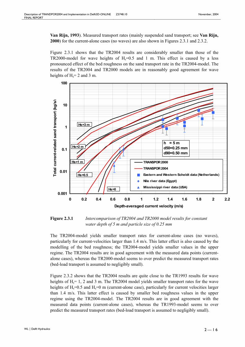
Figures 2.3.1 and 2.3.2 show intercomparison-results of the TR2004-model with TR2000- and TR1993-models based on reference case computations for a water depth of h=5 m and a median particle size of d50= 0.25 mm (see Appendix A of Van Rijn, 1993). The significant wave height varies between 0 and 3 m; the depth-averaged current velocity varies between 0.1 and 2 m/s. The wave-current angle is 90 degrees. Other parameters are: d90= 0.5 mm, water temperature= 15 ˚C and salinity= 30 promille. The TR2004-model results (total sand transport rates) are based on predicted bed roughness and suspended sediment size values, whereas the TR-2000 and TR1993-model results are based on prescribed values in the range of ks=0.02 to 0.1 m and ds= 0.17 to 0.25 mm (see
Description of TRANDPOR2004 and Implementation in Delft3D-ONLINE Z3748.10 November, 2004 FINAL REPORT
WL | Delft Hydraulics 2 — 1 6
Van Rijn, 1993). Measured transport rates (mainly suspended sand transport; see Van Rijn, 2000) for the current-alone cases (no waves) are also shown in Figures 2.3.1 and 2.3.2. Figure 2.3.1 shows that the TR2004 results are considerably smaller than those of the TR2000-model for wave heights of Hs=0.5 and 1 m. This effect is caused by a less pronounced effect of the bed roughness on the sand transport rate in the TR2004-model. The results of the TR2004 and TR2000 models are in reasonably good agreement for wave heights of Hs= 2 and 3 m.
0.001
0.01
0.1
1
10
100
0 0.2 0.4 0.6 0.8 1 1.2 1.4 1.6 1.8 2 2.2
Depth-averaged current velocity (m/s)
Tota
l cur
rent
-rel
ated
san
d tra
nspo
rt (k
g/s/
m
TRANSPOR 2000
TRANSPOR 2004
Eastern and Western Scheldt data (Netherlands)
Nile river data (Egypt)
Mississippi river data (USA)Hs=0
Hs=0.5
h = 5 md50=0.25 mmd90=0.50 mm
Hs=1 m
Hs=2 m
Hs=3 m
Figure 2.3.1 Intercomparison of TR2004 and TR2000 model results for constant
water depth of 5 m and particle size of 0.25 mm The TR2004-model yields smaller transport rates for current-alone cases (no waves), particularly for current-velocities larger than 1.4 m/s. This latter effect is also caused by the modelling of the bed roughness; the TR2004-model yields smaller values in the upper regime. The TR2004 results are in good agreement with the measured data points (current-alone cases), whereas the TR2000-model seems to over predict the measured transport rates (bed-load transport is assumed to negligibly small). Figure 2.3.2 shows that the TR2004 results are quite close to the TR1993 results for wave heights of Hs= 1, 2 and 3 m. The TR2004 model yields smaller transport rates for the wave heights of Hs=0.5 and Hs=0 m (current-alone case), particularly for current velocities larger than 1.4 m/s. This latter effect is caused by smaller bed roughness values in the upper regime using the TR2004-model. The TR2004 results are in good agreement with the measured data points (current-alone cases), whereas the TR1993-model seems to over predict the measured transport rates (bed-load transport is assumed to negligibly small).

Description of TRANDPOR2004 and Implementation in Delft3D-ONLINE Z3748.10 November, 2004 FINAL REPORT
WL | Delft Hydraulics 2 — 1 7
0.001
0.01
0.1
1
10
100
0 0.2 0.4 0.6 0.8 1 1.2 1.4 1.6 1.8 2 2.2
Depth-averaged current velocity (m/s)
Tota
l cur
rent
-rel
ated
san
d tr
ansp
ort (
kg/s
/m
TRANSPOR 1993TRANSPOR 2004Eastern and Western Scheldt data (Netherlands)Nile river data (Egypt)Mississippi river data (USA)Hs=0
Hs=0.5
h = 5 md50=0.25 mmd90=0.50 mm
Hs=1 m
Hs=2 m
Hs=3 m
Figure 2.3.2 Intercomparison of TR2004 and TR1993 model results for constant
water depth of 5 m and particle size of 0.25 mm
2.4 Application of TR2004-model for graded sediment
2.4.1 Experiments
Experiments over a horizontal sand bed have been carried out in a small-scale wave-current flume of the Fluids Mechanics Laboratory of the Delft University of Technology (Jacobs and Dekker, 2000 and Sistermans, 2000). Two types of sand have been used in the experimental program: uniform sand with d50 of about 0.16 mm and graded sand with d50 of about 0.25 mm. The water depth was about 0.5 m in all tests. The hydrodynamic conditions are: irregular waves superimposed on a following current. The significant wave heights are in the range of 0.12 to 0.2 m. The depth-averaged current velocities are in the range of 0.1 to 0.3 m/s (following current). Time-averaged suspended sand concentrations and suspended transport rates have been measured. Instantaneous velocities and sand concentrations at various elevations above the bed have been measured by use of an acoustic instrument. Instantaneous fluid velocities have also been measured by use of an electro-magnetic velocity meter. Time-averaged sand concentration profiles have been obtained by using a pump sampling instrument consisting of 10 intake tubes (internal opening of 3 mm; sampling time of about 20 min).
Description of TRANDPOR2004 and Implementation in Delft3D-ONLINE Z3748.10 November, 2004 FINAL REPORT
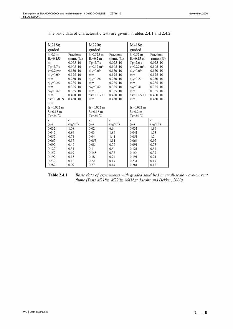
WL | Delft Hydraulics 2 — 1 8
The basic data of characteristic tests are given in Tables 2.4.1 and 2.4.2. M218g graded
M220g graded
M418g graded
h=0.5 m Hs=0.155 m Tp=2.7 s v=0.2 m/s d10=0.09 mm d50=0.26 mm d90=0.42 mm ds=0.1-0.09 mm ∆r=0.022 m λr=0.15 m Te=24 oC
Fractions (mm), (%) 0.075 10 0.105 10 0.130 10 0.175 10 0.230 10 0.285 10 0.325 10 0.365 10 0.400 10 0.450 10
h=0.525 m Hs=0.2 m Tp=2.7 s v=0.17 m/s d10=0.09 mm d50=0.26 mm d90=0.42 mm ds=0.11-0.1 mm ∆r=0.022 m λr=0.18 m Te=24 oC
Fractions (mm), (%) 0.075 10 0.105 10 0.130 10 0.175 10 0.230 10 0.285 10 0.325 10 0.365 10 0.400 10 0.450 10
h=0.52 m Hs=0.15 m Tp=2.6 s v=0.29 m/s d10=0.09 mm d50=0.27 mm d90=0.41 mm ds=0.12-0.1 mm ∆r=0.022 m λr=0.2 m Te=24 oC
Fractions (mm), (%) 0.075 10 0.105 10 0.130 10 0.175 10 0.230 10 0.285 10 0.325 10 0.365 10 0.400 10 0.450 10
z (m)
c (kg/m3)
z (m)
c (kg/m3)
z (m)
c (kg/m3)
0.032 0.042 0.052 0.067 0.092 0.122 0.157 0.192 0.232 0.282
1.08 0.86 0.71 0.57 0.42 0.31 0.19 0.15 0.12 0.09
0.02 0.03 0.04 0.055 0.08 0.11 0.145 0.18 0.22 0.27
6.6 1.86 1.41 1.11 0.72 0.5 0.33 0.24 0.17 0.14
0.031 0.041 0.051 0.066 0.091 0.121 0.156 0.191 0.231 0.281
1.86 1.53 1.2 0.97 0.75 0.54 0.37 0.21 0.17 0.13
Table 2.4.1 Basic data of experiments with graded sand bed in small-scale wave-current
flume (Tests M218g, M220g, M418g; Jacobs and Dekker, 2000)

Description of TRANDPOR2004 and Implementation in Delft3D-ONLINE Z3748.10 November, 2004 FINAL REPORT
WL | Delft Hydraulics 2 — 1 9
M015u uniform
h=0.545 m Hs=0.155 m Tp=2.5 s v=0 m/s
d10=0.12 d50=0.155 d90=0.23 ds=0.13-0.1 (mm)
∆r=0.008 m λr=0.1 m Te=24 oC
z (m)
c (kg/m3)
z (m)
c (kg/m3)
z (m)
c (kg/m3)
0.016 0.026 0.036 0.051 0.076 0.106 0.141
1.15 0.77 0.52 0.26 0.085 0.022 0.0037
0.016 0.026 0.036 0.051 0.076 0.106 0.141
1.42 0.89 0.55 0.28 0.079 0.0184 0.0037
0.011 0.021 0.031 0.046 0.071 0.101 0.136
1.37 0.87 0.60 0.32 0.11 0.028 0.0037
M015g graded
h=0.5 m Hs=0.15 m Tp=2.5 s v=0 m/s
d10=0.08 d50=0.23 d90=0.42 ds=0.08 (mm)
∆r=0.012 m λr=0.09 m Te=24 oC
Fractions (mm), (%) 0.07 10 0.10 10
0.12 10 0.15 10 0.20 10 0.25 10
0.30 10 0.34 10 0.40 10 0.45 10
z (m)
c (kg/m3)
z (m)
c (kg/m3)
z (m)
c (kg/m3)
0.008 0.018 0.028 0.043 0.068 0.098 0.133 0.168 0.208
2 1.35 0.89 0.7 0.38 0.14 0.023 0.009 0.0018
0.008 0.018 0.028 0.043 0.068 0.098 0.133 0.168 0.208
2.3 1.45 1.05 0.79 0.43 0.146 0.0251 0.0072 0.0018
0.005 0.015 0.025 0.04 0.065 0.095 0.13 0.165 0.203
2.47 1.5 1.15 0.93 0.53 0.185 0.031 0.009 0.0018
M018g graded
h=0.5 m Hs=0.18 m Tp=2.7 s v=0 m/s
d10=0.08 d50=0.24 d90=0.42 ds=0.12-0.09 (mm)
∆r=0.012 m λr=0.09 m Te=24 oC
Fractions (mm), (%) 0.07 10 0.10 10
0.12 10 0.15 10 0.20 10 0.25 10
0.30 10 0.34 10 0.40 10 0.45 10
z (m)
c (kg/m3)
z (m)
c (kg/m3)
z (m)
c (kg/m3)
0.021 0.031 0.041 0.056 0.081 0.111 0.146 0.181 0.221 0.271
2.6 1.51 1.03 0.64 0.3 0.11 0.022 0.014 0.0036 0.0018
0.024 0.034 0.044 0.059 0.084 0.114 0.149 0.184 0.224 0.274
4.35 1.41 1.09 0.71 0.36 0.16 0.036 0.0144 0.0036 0.0018
0.025 0.035 0.045 0.06 0.085 0.115 0.15 0.185 0.225 0.275
1.72 1.28 0.99 0.66 0.39 0.18 0.049 0.02 0.0072 0.0018
Table 2.4.2 Basic data of experiments with uniform sand bed and graded sand bed in small-scale wave-current flume (Tests M015u, M015g, M018g; Jacobs and Dekker, 2000)
Description of TRANDPOR2004 and Implementation in Delft3D-ONLINE Z3748.10 November, 2004 FINAL REPORT
WL | Delft Hydraulics 2 — 2 0
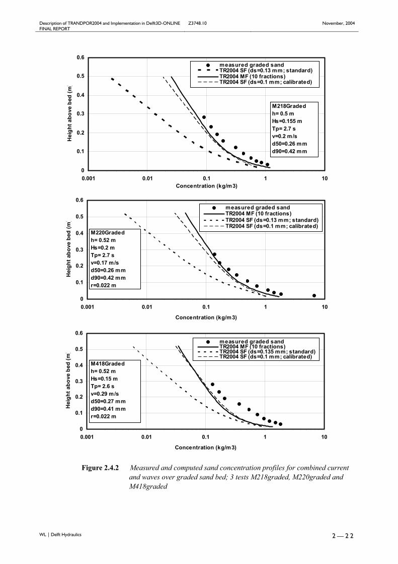
The suspended sand sizes based on analysis in a settling tube, are also given in Tables 2.4.1 and 2.4.2. The measured suspended sand size is about ds= 0.7 to 0.9 d50,bed for the uniform bed materials and about ds= 0.35 to 0.45 d50,bed for the graded bed material. Ripple dimensions have been determined by use of a bed profile follower. Figure 2.4.1 shows measured sand concentration profiles (based on the pumped concentrations) for waves with Hs= 0.15 m and 0.18 m over uniform and graded bed material. The experimental conditions are given in each plot. As can be observed by comparing the results of Figure 2.4.1Top and Middle (Hs=0.15 m for both cases), the near-bed concentrations are significantly larger (factor 2) for the graded sediment bed (Middle) and the sand concentrations higher up in the water column are somewhat larger for the graded sediment bed, which is caused by the winnowing of the fine sediments from the bed. Figure 2.4.2 shows measured concentration profiles for combined wave and current conditions (3 tests). As can be observed, the concentrations are more uniformly distributed over the depth due to the mixing capacity of the current.
2.4.2 Model results
Both the Single-fraction method and the Multi-fraction method have been applied to compute the sand concentration profiles for the 6 experimental cases. The Multi-fraction method has not been used for the uniform sediment case M015U. The results are shown in Figures 2.4.1 and 2.4.2 for 6 cases. The results are: Waves alone (Figure 2.4.1) • the computed sand concentrations based on the SF-method are considerably too small
compared with the measured concentrations in the near-bed region for the uniform sand (Figure 2.4.1Top) due to under-prediction of the reference concentration; the computed concentrations in the upper layers are slightly too large;
• the computed sand concentrations based on the MF-method show reasonably good agreement with the measured concentrations in the near-bed region for the graded sand bed (Figure 2.4.1Middle and Bottom), but the computed concentrations higher up in the water column are much too large compared with the measured values; the winnowing effect of the fine fractions is overestimated by the model; the wave-related mixing coefficient is too large for z>0.1 m.
• the computed reference concentration based on the MF-method is larger than that based on the SF-method, which is in agreement with the physics involved (larger near-bed concentrations for graded sediment than for uniform sediment).
Combined current and waves (Figure 2.4.2) • the computed sand concentrations based on the MF-method show reasonably good
agreement with the measured concentrations for the graded sand; the vertical distribution is predicted rather good, but the reference concentration is somewhat under predicted;
• the computed sand concentrations based on the SF-method are considerably too small if the suspended sediment size is based on the standard prediction method (ds=0.13 mm≅ 0.5d50,bed); the computed sand concentrations show reasonably good agreement with the measured values, if the suspended sediment size is taken (calibrated) as ds= 0.4d50,bed≅ 0.1 mm; the measured suspended sediment sizes vary between ds= 0.35 d50,bed and 0.45 d50,bed.

Description of TRANDPOR2004 and Implementation in Delft3D-ONLINE Z3748.10 November, 2004 FINAL REPORT
WL | Delft Hydraulics 2 — 2 1
Figure 2.4.1 Measured and computed sand concentration profiles for waves (no current)
over uniform sand bed (Top) and graded sand bed (Middle and Bottom); 3 tests M015uniform, M015graded and M018graded
0
0.1
0.2
0.3
0.4
0.5
0.6
0.001 0.01 0.1 1 10
Concentration (kg/m3)
Hei
ght a
bove
bed
(m)
measured uniform sandTR2004 MF
M015Uniformh= 0.54 mHs=0.155 mTp= 2.5 sv=0 m/sd50=0.155 mmd90=0.23 mmr=0.008 m
0
0.1
0.2
0.3
0.4
0.5
0.6
0.001 0.01 0.1 1 10
Concentration (kg/m3)
Hei
ght a
bove
bed
(m)
measured graded sandTR2004 MFTR2004 SF (standard; ds=0.115 mm)
M015Gradedh= 0.5 mHs=0.15 mTp= 2.5 sv=0 m/sd50=0.23 mmd90=0.42 mmr=0.012 m
0
0.1
0.2
0.3
0.4
0.5
0.6
0.001 0.01 0.1 1 10
Concentration (kg/m3)
Hei
ght a
bove
bed
(m)
measured graded sandTR2004 MFTR2004 SF (standard; ds=0.12 mm)
M018Gradedh= 0.5 mHs=0.18 mTp= 2.7 sv=0 m/sd50=0.24 mmd90=0.42 mmr=0.012 m
Description of TRANDPOR2004 and Implementation in Delft3D-ONLINE Z3748.10 November, 2004 FINAL REPORT
WL | Delft Hydraulics 2 — 2 2
Figure 2.4.2 Measured and computed sand concentration profiles for combined current
and waves over graded sand bed; 3 tests M218graded, M220graded and M418graded
0
0.1
0.2
0.3
0.4
0.5
0.6
0.001 0.01 0.1 1 10Concentration (kg/m3)
Hei
ght a
bove
bed
(m)
measured graded sandTR2004 SF (ds=0.13 mm; standard)TR2004 MF (10 fractions)TR2004 SF (ds=0.1 mm; calibrated)
M218Gradedh= 0.5 mHs=0.155 mTp= 2.7 sv=0.2 m/sd50=0.26 mmd90=0.42 mm
0 022
0
0.1
0.2
0.3
0.4
0.5
0.6
0.001 0.01 0.1 1 10
Concentration (kg/m3)
Hei
ght a
bove
bed
(m)
measured graded sandTR2004 MF (10 fractions)TR2004 SF (ds=0.13 mm; standard)TR2004 SF (ds=0.1 mm; calibrated)
M220Gradedh= 0.52 mHs=0.2 mTp= 2.7 sv=0.17 m/sd50=0.26 mmd90=0.42 mmr=0.022 m
0
0.1
0.2
0.3
0.4
0.5
0.6
0.001 0.01 0.1 1 10
Concentration (kg/m3)
Hei
ght a
bove
bed
(m)
measured graded sandTR2004 MF (10 fractions)TR2004 SF (ds=0.135 mm; standard)TR2004 SF (ds=0.1 mm; calibrated)
M418Gradedh= 0.52 mHs=0.15 mTp= 2.6 sv=0.29 m/sd50=0.27 mmd90=0.41 mmr=0.022 m
Description of TRANDPOR2004 and Implementation in Delft3D-ONLINE Z3748.10 November, 2004 FINAL REPORT
WL | Delft Hydraulics 3 — 1
3 Sand transport formulations in DELFT3D model
3.1 Introduction
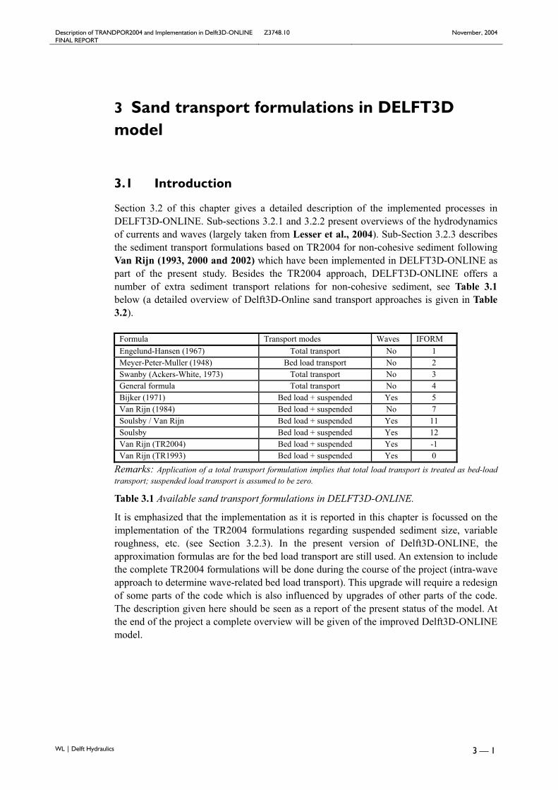
Section 3.2 of this chapter gives a detailed description of the implemented processes in DELFT3D-ONLINE. Sub-sections 3.2.1 and 3.2.2 present overviews of the hydrodynamics of currents and waves (largely taken from Lesser et al., 2004). Sub-Section 3.2.3 describes the sediment transport formulations based on TR2004 for non-cohesive sediment following Van Rijn (1993, 2000 and 2002) which have been implemented in DELFT3D-ONLINE as part of the present study. Besides the TR2004 approach, DELFT3D-ONLINE offers a number of extra sediment transport relations for non-cohesive sediment, see Table 3.1 below (a detailed overview of Delft3D-Online sand transport approaches is given in Table 3.2).
Formula Transport modes Waves IFORM Engelund-Hansen (1967) Total transport No 1 Meyer-Peter-Muller (1948) Bed load transport No 2 Swanby (Ackers-White, 1973) Total transport No 3 General formula Total transport No 4 Bijker (1971) Bed load + suspended Yes 5 Van Rijn (1984) Bed load + suspended No 7 Soulsby / Van Rijn Bed load + suspended Yes 11 Soulsby Bed load + suspended Yes 12 Van Rijn (TR2004) Bed load + suspended Yes -1 Van Rijn (TR1993) Bed load + suspended Yes 0
Remarks: Application of a total transport formulation implies that total load transport is treated as bed-load transport; suspended load transport is assumed to be zero.
Table 3.1 Available sand transport formulations in DELFT3D-ONLINE.
It is emphasized that the implementation as it is reported in this chapter is focussed on the implementation of the TR2004 formulations regarding suspended sediment size, variable roughness, etc. (see Section 3.2.3). In the present version of Delft3D-ONLINE, the approximation formulas are for the bed load transport are still used. An extension to include the complete TR2004 formulations will be done during the course of the project (intra-wave approach to determine wave-related bed load transport). This upgrade will require a redesign of some parts of the code which is also influenced by upgrades of other parts of the code. The description given here should be seen as a report of the present status of the model. At the end of the project a complete overview will be given of the improved Delft3D-ONLINE model.

Description of TRANDPOR2004 and Implementation in Delft3D-ONLINE Z3748.10 November, 2004 FINAL REPORT
WL | Delft Hydraulics 3 — 2
Type of model Spatial dimension
Transport approach
DELFT-ONLINE
2DH Bed load transport a) Wave-averaged transports based on intra-wave transport generated by a intra-wave velocity based on the Isobe-Horikawa method (TR2004) b) Other equilibrium formulations (See Table 2.1.2) Wave-related suspended transport Equilibrium transport based on approximation method of TR2004 Current-related suspended transport 1) Depth-averaged sand concentration derived from equilibrium sand transport formulation plus adjustment factor based on method of Galappatti 2) Equilibrium suspended transport formulations (no adjustment): a)TR2004 (detailed formulations) b)TR2000 (approximation functions) c) Other formulations; see Table 2.1.2 Bed roughness a) specified by user b) roughness predictor
DELFT-ONLINE
3D and 2DV
Bed load transport a) Wave-averaged transports based on intra-wave transport generated by a intra-wave velocity based on the Isobe-Horikawa method (TR2004) b) Other equilibrium formulations (See Table 2.1.2) Wave-related suspended transport Equilibrium transport based on approximation method of TR2004 Current-related suspended transport 1) Concentration derived from advection-diffusion equation 2) Reference concentration derived from a) TR2004 b) Other formulations (Table 2.1.2); ref concentration is calculated backwards from equilibrium suspended transport using computed velocity profiles and mixing coefficient Bed roughness a) specified by user b) roughness predictor
Table 3.2 Sand transport approaches in DELFT-MOR and DELFT3D-ONLINE model.
3.2 Model description
3.2.1 Hydrodynamics
The DELFT3D-FLOW module solves the unsteady shallow-water equations in two (depth-averaged) or three dimensions. The system of equations consists of the horizontal momentum equations, the continuity equation, the transport equation, and a turbulence closure model. The vertical momentum equation is reduced to the hydrostatic pressure relation as vertical accelerations are assumed to be small compared to gravitational acceleration and are not taken into account. This makes the DELFT3D-FLOW model suitable for predicting the flow in shallow seas, coastal areas, estuaries, lagoons, rivers, and lakes. It aims to model flow phenomena of which the horizontal length and time scales are significantly larger than the vertical scales.

Description of TRANDPOR2004 and Implementation in Delft3D-ONLINE Z3748.10 November, 2004 FINAL REPORT
WL | Delft Hydraulics 3 — 3
The user may choose whether to solve the hydrodynamic equations on a Cartesian rectangular, orthogonal curvilinear (boundary fitted), or spherical grid. In three-dimensional simulations a boundary fitted (σ-coordinate) approach is used for the vertical grid direction. For the sake of clarity the equations are presented in their Cartesian rectangular form only. Vertical σ-coordinate system The vertical σ-coordinate is scaled as ( )− ≤ ≤1 0σ
zdζσ
ζ−=+
(3.2.1)
The flow domain of a 3D shallow water model consists of a number of layers. In a σ-coordinate system, the layer interfaces are chosen following planes of constant σ. Thus, the number of layers is constant over the horizontal computational area. For each layer a set of coupled conservation equations is solved. The partial derivatives in the original Cartesian coordinate system are expressed in σ-coordinates by use of the chain rule. This introduces additional terms (Stelling and Van Kester, 1994). Generalised Lagrangian mean (GLM) reference frame In simulations including waves the hydrodynamic equations are written and solved in a GLM reference frame (Andrews and McIntyre, 1978; Groeneweg and Klopman, 1998; and Groeneweg 1999). In GLM formulation the 2DH and 3D flow equations are very similar to the standard Eulerian equations, however, the wave-induced driving forces averaged over the wave period are more accurately expressed. The relationship between the GLM velocity and the Eulerian velocity is given by:
s
s
U u uV v v
= += +
(3.2.2)
where U and V are GLM velocity components, u and v are Eulerian velocity components, and su and sv are the Stokes’ drift components. For details and verification results we refer to Walstra et al. (2000). Hydrostatic pressure assumption Under the so-called “shallow water assumption” the vertical momentum equation reduces to the hydrostatic pressure equation. Under this assumption vertical acceleration due to buoyancy effects or sudden variations in the bottom topography is not taken into account. The resulting expression is:
P g h∂ ρ∂σ
= − (3.2.3)
Horizontal momentum equations The horizontal momentum equations are

Description of TRANDPOR2004 and Implementation in Delft3D-ONLINE Z3748.10 November, 2004 FINAL REPORT
WL | Delft Hydraulics 3 — 4
20
20
1 1
1 1
x x x V
y y y V
U U U U uU v fV P F Mt x y h h
V V V V vU V fU P F Mt x y h h
∂ ∂ ∂ ω ∂ ∂ ∂ν∂ ∂ ∂ ∂σ ρ ∂σ ∂σ
∂ ∂ ∂ ω ∂ ∂ ∂ν∂ ∂ ∂ ∂σ ρ ∂σ ∂σ
+ + + − = − + + +
+ + + − = − + + +
(3.2.4)
in which the horizontal pressure terms, Px and Py , are given by (Boussinesq
approximations)
0
0 0
0
0 0
1
1
x
y
hP g g dx x x
hP g g dy y y
σ
σ
∂ζ ∂ρ ∂σ ∂ρ σρ ∂ ρ ∂ ∂ ∂σ
∂ζ ∂ρ ∂σ ∂ρ σρ ∂ ρ ∂ ∂ ∂σ
′ ′= + + ′
′ ′= + + ′
∫
∫
(3.2.5)
The horizontal Reynold’s stresses, Fx and Fy , are determined using the eddy viscosity
concept (e.g. Rodi, 1984). For large scale simulations (when shear stresses along closed boundaries may be neglected) the forces Fx and Fy reduce to the simplified formulations
2 2 2 2
2 2 2 2x H y HU U V VF Fx y x y
∂ ∂ ∂ ∂ν ν∂ ∂ ∂ ∂
= + = +
(3.2.6)
in which the gradients are taken along σ-planes. In Eq. (3.2.4) Mx and My represent the contributions due to external sources or sinks of momentum (external forces by hydraulic structures, discharge or withdrawal of water, wave stresses, etc.). Continuity equation The depth-averaged continuity equation is given by
hU hVS
t x y∂ ∂∂ζ
∂ ∂ ∂ + + = (3.2.7)
in which S represents the contributions per unit area due to the discharge or withdrawal of water, evaporation, and precipitation. Transport equation The advection-diffusion equation reads
[ ] [ ] [ ] ( )
1H H V
hc hUc hVc ct x y
c c ch D D D hSx x y y h
∂ ∂ ∂ ∂ ω∂ ∂ ∂ ∂σ
∂ ∂ ∂ ∂ ∂ ∂∂ ∂ ∂ ∂ ∂σ ∂σ
+ + + =
+ + +
(3.2.8)
Description of TRANDPOR2004 and Implementation in Delft3D-ONLINE Z3748.10 November, 2004 FINAL REPORT
WL | Delft Hydraulics 3 — 5
in which S represents source and sink terms per unit area. In order to solve these equations the horizontal and vertical viscosity (ν H and νV ) and diffusivity ( DH and DV ) need to be prescribed. In DELFT3D-FLOW the horizontal viscosity and diffusivity are assumed to be a superposition of three parts: 1) molecular viscosity, 2) “3D turbulence”, and 3) “2D turbulence”. The molecular viscosity of the fluid (water) is a constant value O(10-6). In a 3D simulation “3D turbulence” is computed by the selected turbulence closure model (see the turbulence closure model section below). “2D turbulence” is a measure of the horizontal mixing that is not resolved by advection on the horizontal computational grid. 2D turbulence values may either be specified by the user as a constant or space-varying parameter, or can be computed using a sub-grid model for horizontal large eddy simulation (HLES). The HLES model available in DELFT3D-FLOW is based on theoretical considerations presented by Uittenbogaard (1998) and is fully discussed by Van Vossen (2000). For use in the transport equation, the vertical eddy diffusivity is scaled from the vertical eddy viscosity according to
DVV
c
= νσ
(3.2.9)
in which σ c is the Prandtl-Schmidt number given by
σ σ σc c F Ri= 0 b g (3.2.10)
where σ c0 is purely a function of the substance being transported. In the case of the
algebraic turbulence model, F Riσ b g is a damping function that depends on the amount of density stratification present via the gradient Richardson’s number (Simonin et al., 1989). The damping function, F Riσ b g , is set equal to 1.0 if the k −ε turbulence model is used, as
the buoyancy term in the k −ε model automatically accounts for turbulence-damping effects caused by vertical density gradients. We note that the vertical eddy diffusivity used for calculating the transport of “sand” sediment constituents may, under some circumstances, vary somewhat from that given by Eq. (3.2.9) above. The diffusion coefficient used for sand sediment is described in more detail in Section 3.2.3. Turbulence closure models Several turbulence closure models are implemented in DELFT3D-FLOW. All models are based on the so-called “eddy viscosity” concept (Kolmogorov, 1942; Prandtl, 1945). The eddy viscosity in the models has the following form
ν µV c L k= ′ (3.2.11)

Description of TRANDPOR2004 and Implementation in Delft3D-ONLINE Z3748.10 November, 2004 FINAL REPORT
WL | Delft Hydraulics 3 — 6
in which ′cµ is a constant determined by calibration, L is the mixing length, and k is the
turbulent kinetic energy. Two types of turbulence closure models are available in DELFT3D-FLOW. The first is the “algebraic” turbulence closure model that uses algebraic/analytical formulas to determine k and L and therefore the vertical eddy viscosity. The second is the k −ε turbulence closure model in which both the turbulent energy k and the dissipation ε are produced by production terms representing shear stresses at the bed, surface, and in the flow. The “concentrations” of k and ε in every grid cell are then calculated by transport equations. The mixing length L is determined from ε and k according to
L c k kD=
ε (3.2.12)
in which cD is another calibration constant.
3.2.1.1 Boundary Conditions
In order to solve the systems of equations, the following boundary conditions are required: Bed and free surface boundary conditions In the σ-coordinate system the bed and the free surface correspond with σ-planes. Therefore the vertical velocities at these boundaries are simply
ω ω− = =1 0 0 0b g b gand (3.2.13)
Friction is applied at the bed as follows:
1 1
byV bx Vu vh hσ σ
τν ∂ τ ν ∂∂σ ρ ∂σ ρ=− =−
= = (3.2.14)
where bxτ and byτ are bed shear stress components that include the effects of wave-current
interaction. Friction due to wind stress at the water surface may be included in a similar manner. For the transport boundary conditions the vertical diffusive fluxes through the free surface and bed are set to zero. Lateral boundary conditions Along closed boundaries the velocity component perpendicular to the closed boundary is set to zero (a free-slip condition). At open boundaries one of the following types of boundary conditions must be specified: water level, velocity (in the direction normal to the boundary), discharge, or Riemann (weakly reflective boundary condition, Verboom and Slob, 1984). Additionally, in the case of 3D models, the user must prescribe the use of either a uniform or logarithmic velocity profile at inflow boundaries.
Description of TRANDPOR2004 and Implementation in Delft3D-ONLINE Z3748.10 November, 2004 FINAL REPORT
WL | Delft Hydraulics 3 — 7
For the transport boundary conditions we assume that the horizontal transport of dissolved substances is dominated by advection. This means that at an open inflow boundary a boundary condition is needed. During outflow the concentration must be free. DELFT3D-FLOW allows the user to prescribe the concentration at every σ−layer using a time series. For sand sediment fractions the local equilibrium sediment concentration profile may be used.
3.2.1.2 Solution Procedure
DELFT3D-FLOW is a numerical model based on finite differences. To discretise the 3D shallow water equations in space, the model area is covered by a rectangular, curvilinear, or spherical grid. It is assumed that the grid is orthogonal and well-structured. The variables are arranged in a pattern called the Arakawa C-grid (a staggered grid). In this arrangement the water level points (pressure points) are defined in the centre of a (continuity) cell; the velocity components are perpendicular to the grid cell faces where they are situated. Hydrodynamics An alternating direction implicit (ADI) method is used to solve the continuity and horizontal momentum equations (Leendertse 1987). The advantage of the ADI method is that the implicitly integrated water levels and velocities are coupled along grid lines, leading to systems of equations with a small bandwidth. Stelling (1983) extended the ADI method of Leendertse with a special approach for the horizontal advection terms. This approach splits the third-order upwind finite-difference scheme for the first derivative into two second-order consistent discretisations, a central discretisation and an upwind discretisation, which are successively used in both stages of the ADI-scheme. The scheme is denoted as a “cyclic method” (Stelling and Leendertse, 1991). This leads to a method that is computationally efficient, at least second-order accurate, and stable at Courant numbers of up to approximately 10. The diffusion tensor is redefined in the σ-coordinate system assuming that the horizontal length scale is much larger than the water depth (Mellor and Blumberg, 1985) and that the flow is of boundary-layer type. The vertical velocity, ω, in the σ-coordinate system is computed from the continuity equation,
[ ] [ ]hU hVt x y
∂ ∂∂ω ∂ζ∂σ ∂ ∂ ∂
= − − − (3.2.15)
by integrating in the vertical from the bed to a level σ. At the surface the effects of precipitation and evaporation are taken into account. The vertical velocity, ω, is defined at the iso-σ-surfaces. ω is the vertical velocity relative to the moving σ-plane and may be interpreted as the velocity associated with up- or down-welling motions. The vertical velocities in the Cartesian coordinate system can be expressed in the horizontal velocities, water depths, water levels, and vertical coordinate velocities according to:
h h hw U Vx x y y t t
∂ ∂ζ ∂ ∂ζ ∂ ∂ζω σ σ σ∂ ∂ ∂ ∂ ∂ ∂
= + + + + + + (3.2.16)
Description of TRANDPOR2004 and Implementation in Delft3D-ONLINE Z3748.10 November, 2004 FINAL REPORT
WL | Delft Hydraulics 3 — 8
Transport The transport equation is formulated in a conservative form (finite-volume approximation) and is also solved using the so-called “cyclic method” (Stelling and Leendertse, 1991). For steep bottom slopes in combination with vertical stratification, horizontal diffusion along σ-planes introduces artificial vertical diffusion (Huang and Spaulding, 1996). DELFT3D-FLOW includes an algorithm to approximate the horizontal diffusion along z-planes in a σ-coordinate framework (Stelling and Van Kester, 1994). In addition, a horizontal Forester filter (Forester, 1979) based on diffusion along σ-planes is applied to remove any negative concentration values that may occur. The Forester filter is mass conserving and does not inflict significant amplitude losses in sharply peaked solutions.
3.2.2 Waves
3.2.2.1 General
Wave effects can also be included in a DELFT3D-FLOW simulation by running the separate DELFT3D-WAVE module. A call to the DELFT3D-WAVE module must be made prior to running the FLOW module. This will result in a communication file being stored which contains the results of the wave simulation (RMS wave height, peak spectral period, wave direction, mass fluxes, etc) on the same computational grid as is used by the FLOW module. The FLOW module can then read the wave results and include them in flow calculations. Wave simulations may be performed using the 2nd generation wave model HISWA (Holthuijsen et al., 1989) or the 3rd generation SWAN model (Holthuijsen et al., 1993). A significant practical advantage of using the SWAN model is that it can run on the same curvilinear grids as are commonly used for DELFT3D-FLOW calculations; this significantly reduces the effort required to prepare combined WAVE and FLOW simulations. In situations where the water level, bathymetry, or flow velocity field change significantly during a FLOW simulation, it is often desirable to call the WAVE module more than once. The computed wave field can thereby be updated accounting for the changing water depths and flow velocities. This functionality is possible by way of the MORSYS steering module that can make alternating calls to the WAVE and FLOW modules. At each call to the WAVE module the latest bed elevations, water elevations and, if desired, current velocities are transferred from FLOW.
3.2.2.2 Wave Effects
In coastal seas wave action may influence morphology for a number of reasons. The following processes are presently accounted for in DELFT3D-FLOW.
1. Wave forcing due to breaking (by radiation stress gradients) is modelled as a shear stress at the water surface (Svendsen, 1985; Stive and Wind, 1986). This radiation stress gradient is modelled using the simplified expression of Dingemans et al. (1987), where contributions other than those related to the dissipation of wave energy are neglected. This expression is as follows,
Description of TRANDPOR2004 and Implementation in Delft3D-ONLINE Z3748.10 November, 2004 FINAL REPORT
WL | Delft Hydraulics 3 — 9
DM kω
= (3.2.17)
in which M = Forcing due to radiation stress gradients (N/m2), D = Dissipation due to wave breaking (W/m2), ω= Angular wave frequency (rad/s), and k = Wave number vector (rad/m).
2. The effect of the enhanced bed shear stress on the flow simulation is accounted for by following the parameterisations of Soulsby et al. (1993). However, within the present study Delft3D was extended with TR2004 parameterisation which is the used in the simulations presented in this report.
3. The wave-induced mass flux is included and is adjusted for the vertically non-uniform Stokes drift (Walstra et al., 2000).
4. The additional turbulence production due to dissipation in the bottom wave boundary layer and due to wave white capping and breaking at the surface is included as extra production terms in the k −ε turbulence closure model (Walstra et al., 2000).
5. Streaming (a wave-induced current in the bottom boundary layer directed in the direction of wave propagation) is modelled as an additional shear stress acting across the thickness of the bottom wave boundary layer (Walstra et al., 2000).
6. Infragravity wave motions are included following Reniers et al. (2004). 7. The effects of wave asymmetry on the bed shear stresses and sediment transports are
included based on the non-linear wave approximation method of Isobe and Horikawa (1982).
Processes 3, 4, and 5 are essential if the (wave-averaged) effect of waves on the flow is to be correctly represented in 3D simulations. This is especially important for the accurate modelling of sediment transport in a near-shore coastal zone. Reniers et al. (2004) showed that the inclusion of infragravity wave motions (Process 6) are responsible for the development of an alongshore quasi-periodic bathymetry of shoals cut by rip channels. They also showed that the directional spreading of wave energy determines the horizontal alongshore spacing of rip-channel systems to a large extend.
3.2.3 Sediment dynamics and bed level evolution
For the transport of non-cohesive sediment, Van Rijn's (1993, 2000, or 2004) approach is followed by default. The user can also specify a number of other transport formulations (see Table 2.1.1) The transport relations are a mix of Van Rijn’s TRANSPOR2000 (TR2000) and approximation formulations (Van Rijn, 2002; Van Rijn and Walstra, 2003). In all these formulations Van Rijn distinguishes between bed load and suspended load which both have a wave-related and current-related contribution:
, ,
, ,
s s c s w
b b c b w
S S SS S S
= += +
(3.2.18)
in which Ss is the suspended transport, Sb the bed load transport, Ss,c and Ss,w the respective current-related and wave-related suspended transports, Sb,c and Sb,w the respective current-related and wave-related bed load transports. The transport gradients in x- and y-direction

Description of TRANDPOR2004 and Implementation in Delft3D-ONLINE Z3748.10 November, 2004 FINAL REPORT
WL | Delft Hydraulics 3 — 1 0
are being used in the sediment continuity equation to determine the bed level changes, as follows:
( ) ( ), ,, , 0b y s yb x s xbS SS Sz
t x y∂ +∂ +∂ + + =
∂ ∂ ∂ (3.2.19)
with: Sb,x= Sb,c,x+Sb,w,x being the bed-load transport in x-direction (u-velocity direction), Sb,y= Sb,c,y+Sb,w,y being the bed-load transport in y-direction (v-velocity direction), Ss,x= Ss,c,x+Ss,w,x being the suspended load transport in x-direction (u-velocity direction), Ss,y= Ss,c,y+Ss,w,y being the suspended load transport in y-direction (v-velocity direction), and Sb,c and Sb,w are the current-related and wave-related bed load transports, Ss,c and Ss,w are the current-related and wave-related suspended load transports (in x and y directions). The bed-load transport contributions are based on a quasi-steady approach, which implies that the bed-load transport is assumed to respond almost instantaneously to orbital velocities within the wave cycle and to the prevailing current-velocity. Similarly, the wave-related suspended load transport contribution is assumed to respond almost instantaneously to the orbital velocities. These transport contributions (Sb,c, Sb,w and Ss,w) can be formulated in terms of time-averaged (over the wave period) parameters resulting in relatively simple transport expressions. The current-related suspended load transport is based on the variation of the suspended sand concentration field due to the effects of currents and waves. Using a 2DH-approach, the sand concentration field is described in terms of the depth-averaged equilibrium sand concentration derived from equilibrium transport formulations and an adjustment factor based on the (numerical) method of Galappatti. Using a 3D-approach, the sand concentration field is based on the numerical solution of the 3D advection-diffusion equation (see Sub-Section 3.2.3.1). The upgrade of TRANSPOR2000 to TRANSPOR2004 concerns the following points: 1. Predictor of bed roughness, see Eqs. (3.2.36), (3.2.37), (3.2.38) and (3.2.41); 2. Predictor of suspended sediment size, see Eq. (3.2.24); 3. Grain roughness and friction factor, see Eq. (3.2.47); 4. Wave-induced orbital velocities near the bed, see Eq. (3.2.57); 5. Wave-induced bed-shear stress, see Eq. (3.2.51); 6. Shields criterion for fine sand, see Eq. (3.2.54); 7. wave-related suspended transports, see Eq. (3.2.76); 8. Reference concentration, see Eqs. (3.2.34); 9. Modification of the thickness of the effective near-bed sediment mixing layer sδ , see
Eq. (3.2.28); 10. Modification of the thickness of the wave boundary layer wδ , see Eq. (3.2.29);
11. The expressions for the parametric mixing coefficients have also been modified (εs,w,max, εs,w,bed), see Eq. (3.2.27);
12. The wave related efficiency factor (µw), see Eq. (3.2.50).
Description of TRANDPOR2004 and Implementation in Delft3D-ONLINE Z3748.10 November, 2004 FINAL REPORT
WL | Delft Hydraulics 3 — 1 1
3.2.3.1 3-Dimensional advection-diffusion equation for current-related suspended transport
Three-dimensional transport of suspended sediment is calculated by solving the three-dimensional advection-diffusion (mass-balance) equation for the suspended sediment:
( )( ) ( )( ) ( ) ( )
( ) ( ) ( )( ) ( ) ( ), , , 0,
s
s x s y s z
w w cc uc vct x y z
c c cx x y y z z
ε ε ε
∂ −∂ ∂ ∂+ + + +∂ ∂ ∂ ∂
∂ ∂ ∂ ∂ ∂ ∂− − − = ∂ ∂ ∂ ∂ ∂ ∂
(3.2.20)
where:
( )c mass concentration of sediment fraction ( ) [kg/m3],
,u v and w flow velocity components [m/s], ( ) ( ) ( ), , , ,and,s x s y s y s zε ε ε
eddy diffusivities of sediment fraction ( ) [m2/s],
( )sw sediment settling velocity of sediment fraction ( ) ;
hindered settling effects are taken into account [m/s]. The local flow velocities and eddy diffusivities are based on the results of the hydrodynamic computations. Computationally, the three-dimensional transport of sediment is computed in exactly the same way as the transport of any other conservative constituent, such as salinity, heat, and constituents. There are, however, a number of important differences between sediment and other constituents. For example: the exchange of sediment between the bed and the flow, and the settling velocity of sediment under the action of gravity. These additional processes for sediment are obviously of critical importance. Other processes such as the effect that sediment has on the local mixture density, and hence on turbulence damping, can also be taken into account. In addition, if a net flux of sediment from the bed to the flow, or vice versa, occurs then the resulting change in the bathymetry should influence subsequent hydrodynamic calculations. The formulation of several of these processes are sediment-type specific, this especially applies for sand and mud. Based on the computed sand concentration field, the current-related suspended transport rates in x- and y-directions are computed as:
, , ,
, , ,
h
s c x s xa
h
s c y s ya
cS uc dzx
cS vc dzy
ε
ε
∂ = − ∂
∂= − ∂
∫
∫ (3.2.21)
3.2.3.2 Suspended sediment size and sediment settling velocity
The settling velocity of a non-cohesive (“sand”) sediment fraction is computed following the method of Van Rijn (1993). The formulation used depends on the diameter of the sediment in suspension:
Description of TRANDPOR2004 and Implementation in Delft3D-ONLINE Z3748.10 November, 2004 FINAL REPORT
WL | Delft Hydraulics 3 — 1 2
( ) 2
,0
0.5( ) 3
,0 2
0.5( ),0
( 1) , 65 10018
0.01( 1)10 1 1 , 100 1000
1.1 ( 1) , 1000
ss s
ss s
s s s
s g dw m d m
s g dw m d md
w s g d m d
µ µυ
ν µ µυ
µ
−= < ≤
− = + − < ≤
= − <
( )( )
( )( )
( ) ( )
(3.2.22)
where:
( )s relative density of sediment fraction ( ) . ( )d representative diameter of sediment fraction ( ) .
υ kinematic viscosity coefficient of water [m2/s]. The kinematic viscosity is determined using the TR1993 expression which includes the effect of water temperature, Te:
54 1020 eT
υ−⋅=
+ (3.2.23)
If only one sediment fraction is used, the representative diameter of the suspended sediment can be determined based on two options via the user-defined properties SEDDIA (d50 of bed material) and IOPSUS (options for determining sd is determined based on the mobility parameter, ψ , see Eq. (3.2.39), as follows: 1) a suspended sediment diameter based in the following expression:
( )5010, 50
10
50
max 1 0.0006 1 550 550
550
s
s
dd d d ford
d d for
ψ ψ
ψ
= + − − < = ≥
(3.2.24)
2) ds=FACDSS d50; based on a multiplication of the user-defined properties SEDDIA (d50 of bed material) and FACDSS (see also remark)
Remark: In the case of non-uniform bed material Van Rijn (1993) concluded that, on the basis of measurements, ds is in the range of 60% to 100% of d50 of the bed material. If the bed material is very widely graded (well sorted) consideration should be given to using several sediment fractions to model its behaviour more accurately.
3.2.3.3 Sediment mixing and dispersion
DELFT3D-FLOW supports four turbulence closure models: • Constant coefficient. • Algebraic eddy viscosity closure model. • k L− turbulence closure model.

Description of TRANDPOR2004 and Implementation in Delft3D-ONLINE Z3748.10 November, 2004 FINAL REPORT
WL | Delft Hydraulics 3 — 1 3
• k ε− turbulence closure model. The first is a simple constant value which is specified by the user. A constant eddy viscosity will lead to parabolic vertical velocity profiles (laminar flow). The other three turbulence closure models are based on the eddy viscosity concept of Kolmogorov (1942) and Prandtl (1945) and offer zero, first, and second order closures for the turbulent kinetic energy (k) and for the mixing length (L). All three of the more advanced turbulence closure models take into account the effect that a vertical density gradient has on damping the amount of vertical turbulent mixing. The output of a turbulence closure model is the eddy viscosity at each layer interface; from this the vertical sediment mixing coefficient is calculated using the following expressions: Using the algebraic or k-L turbulence model Without waves If the algebraic or k-L turbulence model is selected and waves are inactive then the vertical mixing coefficient for sediment is computed from the vertical fluid mixing coefficient calculated by the selected turbulence closure model. For non-cohesive sediment the fluid mixing coefficient is multiplied by Van Rijn’s ‘beta factor’ which is intended to describe the different diffusivity of a fluid ‘particle’ and a sand grain. Expressed mathematically:
( )s c fε β ε= , (3.2.25)
where:
( )sε vertical sediment mixing coefficient for sediment fraction ( ) .
cβ Van Rijn’s ‘beta’ factor for the sediment fraction.
fε vertical fluid mixing coefficient calculated by the selected turbulence closure model.
Including waves If waves are included in a simulation using the algebraic or k-L turbulence closure model then the sediment mixing coefficient for non-cohesive sediment fractions is calculated entirely separately from the turbulence closure model, using expressions given by Van Rijn (1993) for both the current-related and wave-related vertical turbulent mixing of sediment. The current-related mixing is calculated using the ‘parabolic-constant’ distribution recommended by Van Rijn:
( ), *,
( ), *,
when
when
(1 ) , 0.5 ,
0.25 , 0.5 ,s c c c
s c c c
u z z h z h
u h z h
ε κ β
ε κ β
= − <
= ≥ (3.2.26)
where:
( ),s cε vertical sediment mixing coefficient due to currents (for this sediment
fraction).
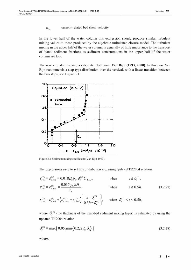
Description of TRANDPOR2004 and Implementation in Delft3D-ONLINE Z3748.10 November, 2004 FINAL REPORT
WL | Delft Hydraulics 3 — 1 4
*,cu current-related bed shear velocity.
In the lower half of the water column this expression should produce similar turbulent mixing values to those produced by the algebraic turbulence closure model. The turbulent mixing in the upper half of the water column is generally of little importance to the transport of ‘sand’ sediment fractions as sediment concentrations in the upper half of the water column are low. The wave- related mixing is calculated following Van Rijn (1993, 2000). In this case Van Rijn recommends a step type distribution over the vertical, with a linear transition between the two steps, see Figure 3.1.
Figure 3.1 Sediment mixing coefficient (Van Rijn 1993).
The expressions used to set this distribution are, using updated TR2004 relation:
( )
( ) ( ) ( ) ( ), , , ,
( ) ( ), ,max
( )( ) ( ) ( ) ( ) ( ), , ,max , ( )
when
when
when
0.018 , ,0.035 , 0.5 ,
, 0.5 ,0.5
s w s bed w br s w r s
br ss w s
p
ss w s bed s s bed s
s
U zhH z h
T
z z hh
δε ε β γ δ δγε ε
δε ε ε ε δδ
= = ≤
= = ≥
−= + − < < −
(3.2.27)
where ( )sδ (the thickness of the near-bed sediment mixing layer) is estimated by using the
updated TR2004 relation:
{ }( ) max 0.05,min 0.2,2s br wδ γ δ= (3.2.28)
where:
Description of TRANDPOR2004 and Implementation in Delft3D-ONLINE Z3748.10 November, 2004 FINAL REPORT
WL | Delft Hydraulics 3 — 1 5
wδ thickness of the wave boundary layer (updated TR2004 relation): 0.25
, ,
0.36ws w r
AAk
δδδ
−
=
(3.2.29)
brγ empirical coefficient related to wave breaking: 0.5
1 0.4 1 0.4s sbr br
H Hand forh h
γ γ = + − = ≤
(3.2.30)
, ,s w rk wave-related bed roughness (as calculated for suspended sediment transport, see Eq. (3.2.41)).
The total vertical sediment mixing coefficient according to Van Rijn is based on the sum of the squares:
( ) ( )2 ( )2, ,s s c s wε ε ε= + , (3.2.31)
where sε is the vertical sediment diffusion coefficient used in the suspended sediment transport calculations for this sediment fraction. Using the k ε− turbulence model In the case of the k ε− turbulence closure model the vertical sediment mixing coefficient can be calculated directly from the vertical fluid mixing coefficient calculated by the turbulence closure model, using the following expression:
( ) ( )s cw fε β ε= , (3.2.32)
where: ( )sε vertical sediment mixing coefficient of sediment fraction ( ) . ( )cwβ the effective Van Rijn’s ‘beta’ factor of sediment fraction ( ) . It consists of a
wave and current related contribution: 2
( )( )
,
1 2 .scw
cw
wu
β∗
= +
(3.2.33)
*,cwu combined wave and current-related shear velocity
fε vertical fluid mixing coefficient calculated by the k ε− turbulence closure model
This implies that the value of ( )cwβ is space (and time) varying, however it is constant over
the depth of the flow. In addition, due to the limited knowledge of the physical processes involved, the beta-factor ( )
cwβ is limited to the range ( )1 1.5cwβ< < .

Description of TRANDPOR2004 and Implementation in Delft3D-ONLINE Z3748.10 November, 2004 FINAL REPORT
WL | Delft Hydraulics 3 — 1 6
Remark: The k ε− turbulence closure model has been extended by Walstra et al. (2000) to include the three-dimensional effects of waves on the mixing (via the frictional bottom dissipation and wave breaking dissipation).
3.2.3.4 Reference concentration
For non-cohesive sediment (e.g. sand), we follow the method of Van Rijn (1993) for the combined effect of waves and currents. The reference height is updated for TR2004 and now reads:
( ), , , ,max 0.5 ,0.5 ,0.01s c r s w ra k k= , (3.2.34)
where:
a Van Rijn’s reference height.
, ,s c rk current-related bed roughness height due to small-scale ripples (see options below).
, ,s w rk
wave-related bed roughness height due to small-scale ripples (see options below).
The total physical current-related roughness kc is calculated as:
( )0.52 2 2, , , , , , ,s c s c r s c mr s c dk k k k= + + (3.2.35)
which is based on a summation of the current-related roughness due to ripples ( , ,s c rk ),
mega-ripples ( , ,s c mrk ) and dunes ( , ,s c dk , rivers only).
The current-related roughness due to ripples is estimated as:
( ), , 50
, , 50
, , 50
150 0 50 ( , )
182.5 0.65 50 250 ( , )
20 250 ( )
s c r
s c r
s c r
k d and lower wave current regime SWR ripples
k d and upper wave current regime sheet flow
k d and linear approach in transitional regime
ψ
ψ ψ
ψ
= ≤ ≤ −
= − < < −
= ≥
(3.2.36)
The current-related roughness due to mega-ripples reads:
( ), ,
, ,
, ,
, ,
0.0002 0 50 1
0.011 0.00002 50 550 10 550 1
0.02 0.2
s c mr
s c mr
s c mr
s c mr
k h and and h
k h and and hk and and h
k
ψ ψψ ψ
ψ
= ≤ ≤ >
= − < < >= ≥ >
≤ ≤
(3.2.37)
The current-related roughness due to dunes in rivers reads:

Description of TRANDPOR2004 and Implementation in Delft3D-ONLINE Z3748.10 November, 2004 FINAL REPORT
WL | Delft Hydraulics 3 — 1 7
( ), ,
, ,
, ,
, ,
0.0004 0 100 1
0.048 0.00008 100 600 10 600 1
0.02 1.0
s c d
s c d
s c d
s c d
k h and and h
k h and and hk and and h
k
ψ ψψ ψ
ψ
= ≤ ≤ >
= − < < >= ≥ >
≤ ≤
(3.2.38)
in which ψ is the mobility parameter:
( )2
501wcu
s gdψ =
−, (3.2.39)
where:
2 2,wc r Ru U vδ= + , (3.2.40)
in which Uδ,r is the representative peak orbital velocity near bed based on the non-linear wave theory of Isobe-Horikawa, see Equation (3.2.57), Rv is the magnitude of an equivalent depth-averaged velocity computed from the velocity in the bottom computational layer, assuming a logarithmic velocity profile. In line with this, it is proposed that the physical wave-related roughness of small-scale ripples is given by:
( )
, , 50
, , 50
, , 50
150 50(lower wave-current regime, SWR ripples)20 250(upper wave-current regime, sheet flow)
182.5 0.65 50 250(linear approach in transitional regime)
s w r
s w r
s w r
k d fork d for
k d for
ψψ
ψ ψ
= ≤= ≥
= − < <
(3.2.41)
This predictor is assumed to be valid for relatively fine sand with d50 in the range of 0.1 to 0.5 mm. An estimate of the bed roughness for coarse particles (d50>0.5 mm) can be obtained by using Eq. (3.2.41) for d50=0.5 mm. Thus, d50=0.5 mm for d50≥0.5 mm resulting in a maximum bed roughness height of 0.075 m (upper limit). The lower limit will be ks,w,r=15d50= 0.0015 m for sand with d50≤0.1 mm. Larger scale wave-induced ripples (often known as ‘long wave ripples’ may be present, but the physical roughness of these types of ripples is assumed to be zero, as flow separation is not likely to occur. Calculation of the reference concentration The reference concentration is calculated in accordance with Van Rijn (2000), but an additional factor η is introduced (and monitored) to reflect the presence of multiple sediment fractions. The resulting expression is:
( )( )
1.5( ) ( )50( ) ( ) ( )
s 0.3( ) 0.015 a
a SUS
d Tc f
a Dη ρ
∗
= (3.2.42)
Description of TRANDPOR2004 and Implementation in Delft3D-ONLINE Z3748.10 November, 2004 FINAL REPORT
WL | Delft Hydraulics 3 — 1 8
where:
( )ac mass concentration at reference height a.
fSUS multiplication factor specified in the morphological input file. In order to evaluate this expression the following quantities must be calculated:
( )η relative availability of sediment fraction:
( ) mass of fraction ( ) in mixing layer
total mass of sediment in mixing layerη = . (3.2.43)
( )D∗ non-dimensional particle diameter: 1
( ) 3( ) ( )
50 2
( 1)s gD dυ∗
−=
. (3.2.44)
( )aT non-dimensional bed-shear stress:
( ) ( ) ( )( ) , ,
( )
( )c b cw w b w cra
cr
Tµ τ µ τ τ
τ+ −
= . (3.2.45)
( )cµ efficiency factor current:
( )( ) cc
c
ff
µ ′= . (3.2.46)
( )cf ′ gain related friction factor:
2
( )10 ( )
90
120.24 logchf
d
− ′ =
. (3.2.47)
( )cf total current-related friction factor:
2
( )10
,
120.24 logcs c
hfk
−
= . (3.2.48)
,b cwτ bed shear stress due to current in the presence of waves. Note that the bed shear velocity *u is calculated in such a way that Van
Rijn’s wave-current interaction factor cwα is not required. 2
, *b cw w uτ ρ= , (3.2.49)( )wµ efficiency factor waves was recalibrated for the TR2004 formula:
( )
*( )
, *
( ), *
0.7
0.35 2
0.14 5
w
w MAX
w MIN
D
for D
for D
µ
µ
µ
=
= <
= >
, (3.2.50)
,b wτ bed shear stress due to waves (updated in TR2004):
( )2, ,
14b w w w rf Uδτ ρ= (3.2.51)

Description of TRANDPOR2004 and Implementation in Delft3D-ONLINE Z3748.10 November, 2004 FINAL REPORT
WL | Delft Hydraulics 3 — 1 9
wf total wave-related friction factor: 0.19
, ,
exp 6 5.2ws w r
Afk
δ
− = − +
. (3.2.52)
( )crτ critical bed shear stress:
( ) ( )3( ) ( ) ( ) ( )501cr mud s w crp gdτ ρ ρ θ= + − . (3.2.53)
( )crθ threshold parameter ( )
crθ is calculated according to the classical Shields curve as modelled by Van Rijn (1993) as a function of the non-dimensional grain size D*. This avoids the need for iteration. Note that, for clarity, in this expression the symbol D∗ has been used where ( )D∗ would be more correct:
( ) 0.5* *
( ) 0.64* *
( ) 0.1* *
( ) 0.29* *
( )*
0.115 , 1 4
0.14 , 4 10
0.04 , 10 20
0.013 , 20 150
0.055, 150
cr
cr
cr
cr
cr
D D
D D
D D
D D
D
θθθθθ
−
−
−
= < ≤
= < ≤
= < ≤
= < ≤
= <
(3.2.54)
a Van Rijn’s reference height:
( ), , , ,max 0.5 ,0.5 ,0.01s c r s w ra k k= (3.2.55)
Aδ peak orbital excursion at the bed: ˆ
2pT U
A δδ π= (3.2.56)
( )50d representative sediment diameter. ( )90d 90% sediment passing size.
h water depth.
ak
apparent bed roughness felt by the flow when waves are present. Calculated by DELFT3D-FLOW using the wave-current interaction formulation selected.
,10a s ck k≤ .
,s ck current-related roughness.
, ,s w rk wave-related roughness.
zu velocity magnitude taken from a near-bed computational layer. In a current-only situation the velocity in the bottom computational layer is used. Otherwise, if waves are active, the velocity is taken from the layer closest to the height of the top of the wave mixing layer, wδ .
,rUδ peak orbital velocity at the bed (updated TR2004 relation):
( ) ( )( )1
3 3 3, , ,0.5 0.5r for backU U Uδ δ δ= + (3.2.57)
uz height above bed of the near-bed velocity ( )zu used in the calculation of bottom shear stress due to current.

Description of TRANDPOR2004 and Implementation in Delft3D-ONLINE Z3748.10 November, 2004 FINAL REPORT
WL | Delft Hydraulics 3 — 2 0
r∆ estimated ripple height, see Eq. (B.8.32)
mδ
thickness of wave boundary mixing layer following (updated TR2004 relation):
, ,2 0.05 0.2m w m MIN m MAXwith andδ δ δ δ= = = (3.2.58)
wδ wave boundary layer thickness (updated in TR2004): 0.25
, ,
0.36ws w r
AAk
δδδ
−
=
(3.2.59)
We emphasise the following points regarding this implementation: • The bottom shear stress due to currents is based on a near-bed velocity taken from the
hydrodynamic calculations, rather than the depth-averaged velocity used by Van Rijn. • All sediment calculations are based on hydrodynamic calculations from the previous half
time-step. We find that this is necessary to prevent unstable oscillations developing. If Van Rijn’s reference height a lies below the centre of the lowest computational cell (zkmxc) that lies above Van Rijn’s reference height a, the concentration at zkmxc is computed following the conventional methods of TR2004. This concentration will now serve as the new reference concentration and the new reference height will consequently be located at zkmxc. The reason for this approach is that vertical concentration gradients at the reference height are often too great to accurately predict sediment source and sink terms for the reference layer (see Paragraph 3.2.4). This is especially important in deep water where the thickness of the bottom cell is often much greater than the reference height.
3.2.4 Erosion and deposition
The transfer of sediment between the bed and water column is modelled using sink and source terms acting on the near-bottom layer that is entirely above Van Rijn’s reference height. This layer is identified as the reference layer and for brevity is referred to as the kmx layer;
BED
a
BED
Layerkmx
BED
kmx
kmx
kmx
Coarse Grid Medium Grid Fine Grid
Standard computational cell
Reference cell for “sand” sediment
Concentration set equal to concentration of reference layer for‘sand’ sediment calculations
KEY
Figure 3.2 Selection of the kmx layer.

Description of TRANDPOR2004 and Implementation in Delft3D-ONLINE Z3748.10 November, 2004 FINAL REPORT
WL | Delft Hydraulics 3 — 2 1
The sediment concentration in the layer(s) that lie below the kmx layer are assumed to rapidly adjust to the same concentration as the reference layer. Each half time-step the source and sink terms model the quantity of sediment entering the flow due to upward diffusion from the reference level and the quantity of sediment dropping out of the flow due to sediment settling. A sink term is solved implicitly in the advection-diffusion equation, whereas a source term is solved explicitly. The required sink and source terms for the kmx layer are calculated as follows.
cwFluxDeposition s=
az∆
dzdcFluxErosion sε=
kmxlayer
BED Figure 3.3 Schematic arrangement of flux bottom boundary condition.
In order to determine the required sink and source terms for the kmx layer, the concentration and concentration gradient at the bottom of the kmx layer need to be approximated. We assume a standard Rouse profile between the reference level a and the centre of the kmx layer (see Figure 3.4).
( )
( ) ( ) ( )( )a
Aa h zc cz h a
−= − , (3.2.60)
where:
)(c concentration of sediment fraction (ℓ). )(
ac reference concentration of sediment fraction (ℓ). a Van Rijn’s reference height. h water depth. z elevation above the bed. )(A Rouse number. As the reference concentration and the concentration in the centre of the kmx layer ckmx are known, the exponent A(ℓ) can be determined.
−
−
=⇒
−
−=
)()(ln
ln
)()( )(
)(
)()(
ahzzha
cc
AA
ahzzhacc
kmx
kmx
a
kmx
kmx
kmxakmx (3.2.61)
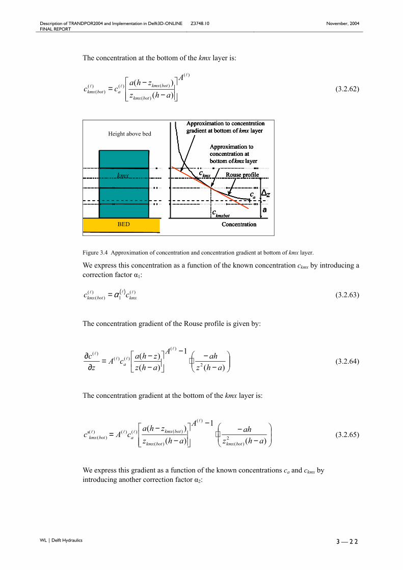
Description of TRANDPOR2004 and Implementation in Delft3D-ONLINE Z3748.10 November, 2004 FINAL REPORT
WL | Delft Hydraulics 3 — 2 2
The concentration at the bottom of the kmx layer is:
)(
)(
)()()()( )(
)( A
ahzzha
ccbotkmx
botkmxabotkmx
−−
= (3.2.62)
a
BED
kmx +
+∆z
ckmx
ca
Concentration
Approximation to concentrationgradient at bottom of kmx layer
Approximation toconcentration atbottom of kmx layer
ckmxbot
Rouse profile
a
BED
kmx +
+∆z
ckmx
ca
Concentration
Approximation to concentrationgradient at bottom of kmx layer
Approximation toconcentration atbottom of kmx layer
ckmxbot
Rouse profile
a
BED
kmx +
+∆z
ckmx
ca
Concentration
Approximation to concentrationgradient at bottom of kmx layer
Approximation toconcentration atbottom of kmx layer
ckmxbot
Rouse profile
a
BED
kmx
a
BED
kmx +
+∆z
ckmx
ca
Concentration
Approximation to concentrationgradient at bottom of kmx layer
Approximation toconcentration atbottom of kmx layer
Height above bed
ckmxbot
Rouse profile
Figure 3.4 Approximation of concentration and concentration gradient at bottom of kmx layer.
We express this concentration as a function of the known concentration ckmx by introducing a correction factor α1:
( )( ) ( )( ) 1kmx bot kmxc cα= (3.2.63)
The concentration gradient of the Rouse profile is given by:
−
−⋅−
−−=
∂∂
)(
1
)()(
2
)(
)()()(
ahzahA
ahzzhacA
zc
a (3.2.64)
The concentration gradient at the bottom of the kmx layer is:
−−⋅
−
−−
=)(
1
)()(
' 2)(
)(
)(
)()()()()( ahz
ahA
ahzzha
cAcbotkmxbotkmx
botkmxabotkmx (3.2.65)
We express this gradient as a function of the known concentrations ca and ckmx by introducing another correction factor α2:
Description of TRANDPOR2004 and Implementation in Delft3D-ONLINE Z3748.10 November, 2004 FINAL REPORT
WL | Delft Hydraulics 3 — 2 3
( )( ) ( )
( )( ) 2' kmx a
kmx botc cc
zα −= ∆
(3.2.66)
Erosive flux due to upward diffusion The upward diffusion of sediment through the bottom of the kmx layer is given by the expression:
( ) ( )( )
scEz
ε ∂=∂
, (3.2.67)
where ( )sε and
( )cz
∂∂
are evaluated at the bottom of the kmx layer.
We approximate this expression by:
( ) ( ) ( )( ) ( )
2a kmx
sc cE
zα ε
−≈ ∆ , (3.2.68)
where: ( )
2α correction factor for sediment concentration ( )sε sediment diffusion coefficient evaluated at the bottom of the kmx cell of
sediment fraction ( ) . ( )ac reference concentration of sediment fraction ( ) . ( )kmxc average concentration of the kmx cell of sediment fraction ( ) .
z∆ difference in elevation between the centre of the kmx cell and Van Rijn’s reference height:
kmxz z a∆ = − . The erosion flux is split in a source and sink term:
( )( ) ( ) ( ) ( ) ( ) ( )2 2s a s kmxc cE
z zα ε α ε≈ −
∆ ∆ (3.2.69)
The first of these terms can be evaluated explicitly and is implemented as a sediment source term. The second can only be evaluated implicitly and is implemented as a (positive) sink term. Thus:
( )( ) ( ) ( )
( )( ) ( ) ( )
2
2
s aerosion
s kmxerosion
cSourcez
cSinkz
α ε
α ε
=∆
=∆
(3.2.70)

Description of TRANDPOR2004 and Implementation in Delft3D-ONLINE Z3748.10 November, 2004 FINAL REPORT
WL | Delft Hydraulics 3 — 2 4
Deposition flux due to sediment settling The settling of sediment through the bottom of the kmx cell is given by the expression:
( ) ( ) ( )( )s kmx botD w c= , (3.2.71)
where ( )sw and ( )
( )kmx botc are evaluated at the bottom of the kmx layer.
We set:
( ) ( ) ( )( ) 1kmx bot kmxc cα= (3.2.72)
The deposition flux is approximated by:
( ) ( ) ( ) ( )1 kmx sD c wα≈ (3.2.73)
This results in a simple deposition sink term:
( ) ( ) ( ) ( )1deposition kmx sSink c wα= (3.2.74)
The total source and sink terms is given by:
( ) ( ) ( )( )
( ) ( ) ( )( )
( ) ( ) ( )
2
2 1
,
.
sa
skmx kmx s
Source cz
Sink c c wz
εα
εα α
= ∆
= + ∆
(3.2.75)
These source and sink terms are positive definite.
3.2.5 Wave-related suspended transport
The wave-related suspended transport is an estimation of the suspended sediment transport due to wave velocity asymmetry effects. This is intended to model the effect of asymmetric wave orbital velocities on the transport of suspended material within about 0.5m of the bed (the bulk of the suspended transport affected by high frequency wave oscillations). This wave-related suspended sediment transport is modelled using an approximation method proposed by Van Rijn (2002):
, SUSWs w A TS f U Lγ= (3.2.76)
where:
,s wS = wave-related suspended transport (kg/m/s)
SUSWf = user specified tuning parameter γ = phase lag coefficient which is set to 0.1 (was 0.2 in TR2000)
Description of TRANDPOR2004 and Implementation in Delft3D-ONLINE Z3748.10 November, 2004 FINAL REPORT
WL | Delft Hydraulics 3 — 2 5
AU = velocity asymmetry value (m/s) = 4 4, ,
3 3, ,
for back
for back
U UU U
δ δ
δ δ
−+
TL = the approximated suspended sediment load (kg/m2):
500.007T s eL d Mρ= (3.2.77)
in which Me is the excess sediment mobility number due to waves and currents (-):
( )( )
2
501eff cr
e
v vM
s gd−
=−
(3.2.78)
and:
2 2,eff R forv v Uδ= + (3.2.79)
in which:
crv = critical depth averaged velocity for initiation of motion (based on a parameterisation of the Shields curve) (m/s).
Rv = magnitude of an equivalent depth-averaged velocity computed from the velocity in the bottom computational layer, assuming a logarithmic velocity profile (m/s).
, forUδ = near-bed peak orbital velocity (m/s) in the direction on wave propagation based on
the significant wave height.
,backUδ = near-bed peak orbital velocity (m/s) opposite the direction on wave propagation
based on the significant wave height.
, forUδ and ,backUδ are the high frequency near-bed orbital velocities due to short waves and
are computed using a modification of the method of Isobe and Horikawa (1982). This method is a parameterisation of fifth-order Stokes wave theory and third-order cnoidal wave theory which can be used over a wide range of wave conditions and takes into account the non-linear effects that occur when waves propagate in shallow water (Grasmeijer and Van Rijn, 1999). The streaming velocity is not included in the implementation. In Delft3D the streaming is included as an additional shear stress distributed linearly across the wave boundary layer and is therefore included in vR (Walstra et al., 2000). The wave-related suspended transport components in x- and y-directions are:
, , ,
, , ,
cossin
s w x s w
s w y s w
S SS S
φφ
==
(3.2.80)
Description of TRANDPOR2004 and Implementation in Delft3D-ONLINE Z3748.10 November, 2004 FINAL REPORT
WL | Delft Hydraulics 3 — 2 6
3.2.6 Bed load transport
Bed-load transport is calculated for all “sand” sediment fractions by following the TR2004 approach. This accounts for the near-bed sediment transport occurring below the reference height a described above. The approach first computes the magnitude and direction of the bed-load “sand” transport using TR2004. The computed sediment transport vectors are then relocated from water-level points to velocity points using an “upwind” computational scheme to ensure numerical stability. Finally the transport components are adjusted for bed-slope effects. Here the transport formulations are highlighted, more information on numerical aspects and bed slope effects can be found in the DELFT3D user manual. The net bed-load transport rate in conditions with uniform bed material is obtained by time-averaging (over the wave period T) of the instantaneous transport rate using the bed-load transport model (quasi-steady approach), as follows:
,1
b b tS S dtT = ∫ (3.2.81)
with Sb,t = F(instantaneous hydrodynamic and sediment transport parameters). The formula applied, reads as:
( )0.5 '', , ,, ,0.3
, 50 *,
max 0,0.5 b cw t b crb cw t
b t sb cr
S d Dτ ττ
ρρ τ
− − =
(3.2.82)
in which: τ/b,cw,t = instantaneous grain-related bed-shear stress due to both current and wave motion =
0.5 ρ f/cw (Uδ,cw,t)2,
Uδ,cw,t = instantaneous velocity due to current and wave motion at reference height a, see Equation (3.2.34),
f/c = current-related grain friction coefficient =0.24(log(12h/ks,grain))-2,
f/w = wave-related grain friction coefficient=Exp[-6+5.2(Aδ/ks,grain)-0.19],
α = coefficient related to relative strength of wave and current motion:ˆ
ˆR
UU v
δ
δ
α =+
,
Uδ = the peak orbital velocity, vR is the equivalent current velocity calculated at reference height a,
βf = coefficient related to vertical structure of velocity profile, Aδ = peak orbital excursion, τb,cr = critical bed-shear stress according to Shields, ρs = sediment density, ρ = fluid density, d50 = particle size, D* = dimensionless particle size.
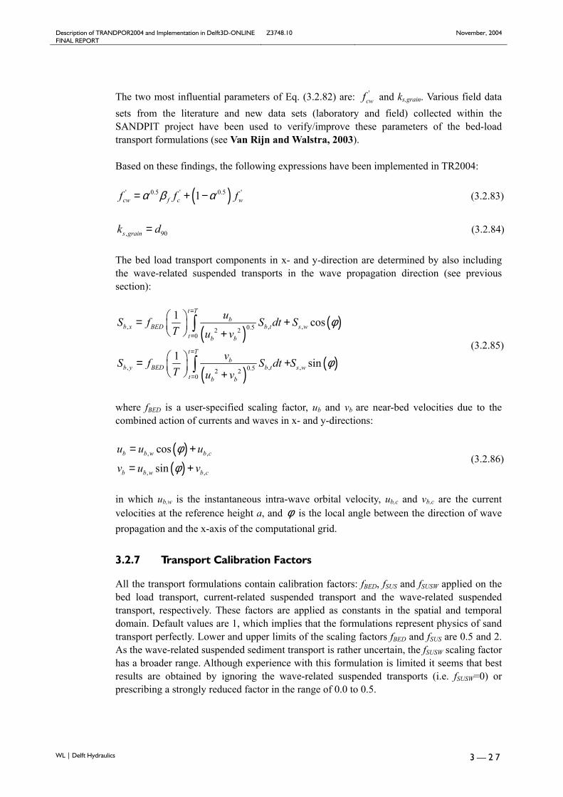
Description of TRANDPOR2004 and Implementation in Delft3D-ONLINE Z3748.10 November, 2004 FINAL REPORT
WL | Delft Hydraulics 3 — 2 7
The two most influential parameters of Eq. (3.2.82) are: '
cwf and ks,grain. Various field data sets from the literature and new data sets (laboratory and field) collected within the SANDPIT project have been used to verify/improve these parameters of the bed-load transport formulations (see Van Rijn and Walstra, 2003). Based on these findings, the following expressions have been implemented in TR2004:
( )' 0.5 ' 0.5 '1cw f c wf f fα β α= + − (3.2.83)
, 90s graink d= (3.2.84)
The bed load transport components in x- and y-direction are determined by also including the wave-related suspended transports in the wave propagation direction (see previous section):
( )( )
( )( )
, , ,0.52 20
, , ,0.52 20
1 cos
1 sin
t Tb
b x BED b t s wt b b
t Tb
b y BED b t s wt b b
uS f S dt ST u v
vS f S dt ST u v
φ
φ
=
=
=
=
= + +
= + +
∫
∫ (3.2.85)
where fBED is a user-specified scaling factor, ub and vb are near-bed velocities due to the combined action of currents and waves in x- and y-directions:
( )( )
, ,
, ,
cos
sinb b w b c
b b w b c
u u u
v u v
φφ
= +
= + (3.2.86)
in which ub,w is the instantaneous intra-wave orbital velocity, ub,c and vb,c are the current velocities at the reference height a, and φ is the local angle between the direction of wave propagation and the x-axis of the computational grid.
3.2.7 Transport Calibration Factors
All the transport formulations contain calibration factors: fBED, fSUS and fSUSW applied on the bed load transport, current-related suspended transport and the wave-related suspended transport, respectively. These factors are applied as constants in the spatial and temporal domain. Default values are 1, which implies that the formulations represent physics of sand transport perfectly. Lower and upper limits of the scaling factors fBED and fSUS are 0.5 and 2. As the wave-related suspended sediment transport is rather uncertain, the fSUSW scaling factor has a broader range. Although experience with this formulation is limited it seems that best results are obtained by ignoring the wave-related suspended transports (i.e. fSUSW=0) or prescribing a strongly reduced factor in the range of 0.0 to 0.5.

Description of TRANDPOR2004 and Implementation in Delft3D-ONLINE Z3748.10 November, 2004 FINAL REPORT
WL | Delft Hydraulics 3 — 2 8
3.3 Implementation Check of TR2004 in Delft3D
The implementation of the TR2004 formulations is checked by performing a comparison between the original TR2004 point model and the updated Delft3D model for a number of idealized cases. The cases have been selected so that they are in the validity range of both models. Only stationary cases are considered in which the water depth was kept constant at 5 m, but with an increasing current velocity: from 0 to 2 m/s with a 0.25 m/s interval. For each of these nine current conditions three wave conditions were run (Hs = 0 m, Hs = 1 m and Hs = 2 m) with five angles between the currents and the waves (0˚ - waves following the current, 45˚, 90˚, 135˚ and 180˚ - waves opposing the current). So in total 135 different combinations of currents, waves and angle between currents and waves were considered. In all simulations the TR2004 formulation was used with defaults values (e.g. no scaling of transports) and settings (e.g. using the predictors for bed roughness and the suspended sediment diameter). The sediment characteristics are: D10 = 150 µm, D50 = 200 µm, D90 = 300 µm. The results are presented in Figure 3.5 to Figure 3.9. Each figure represents a wave-current angle and contains 6 plots displaying: reference concentration (top left), suspended sediment transport (top right), bed load transport (middle left), suspended sediment diameter (middle right), bed roughness (bottom left) and apparent roughness (bottom right) which are all plotted as a function of the current velocity. It can be seen that for all the considered cases the agreement between the TR2004 point model and the updated Delft3D is very good. For some parameters small differences can be observed, but the concentration, suspended load and bed load transports are always in good agreement. Based on these comparisons it was concluded that the TR2004 has been implemented in Delft3D with sufficient accuracy.
3.4 Miscellaneous Improvements to Delft3D
Apart from the implementation of the TR2004 formulations a number of other improvements and extensions have been added to the code: • Implementation of Snell’s law in the wave and roller energy equations which are solved
in Flow-module which allows the Delft3D-model to be run in profile mode. • Inclusion of the Ruessink et al. (2003) γ-expression in wave energy equation which
results in a significant improved wave prediction over breaker bars in the surf zone. • Implementation of the breaker delay concepts of Roelvink et al. (1995) which is based
on a modification of the local maximum wave height and Reniers et al. (2004) which is based on a delayed response of the wave induced mass flux (or undertow).
• Minor improvements: mainly related to the removal of small inconsistencies (e.g. consistent calculation of the imaginary depth-averaged velocity using the velocity in the lowest layer and a logarithmic velocity distribution) and enhancement of the numerical stability of the model (e.g. limiting the source and sink terms in the transport advection-diffusion equations to a user-prescribed percentage of the local water depth).
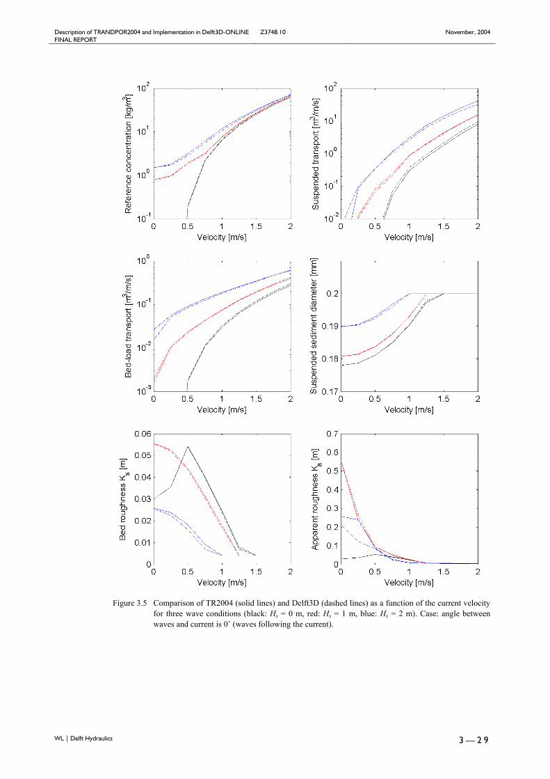
Description of TRANDPOR2004 and Implementation in Delft3D-ONLINE Z3748.10 November, 2004 FINAL REPORT
WL | Delft Hydraulics 3 — 2 9
Figure 3.5 Comparison of TR2004 (solid lines) and Delft3D (dashed lines) as a function of the current velocity
for three wave conditions (black: Hs = 0 m, red: Hs = 1 m, blue: Hs = 2 m). Case: angle between waves and current is 0˚ (waves following the current).
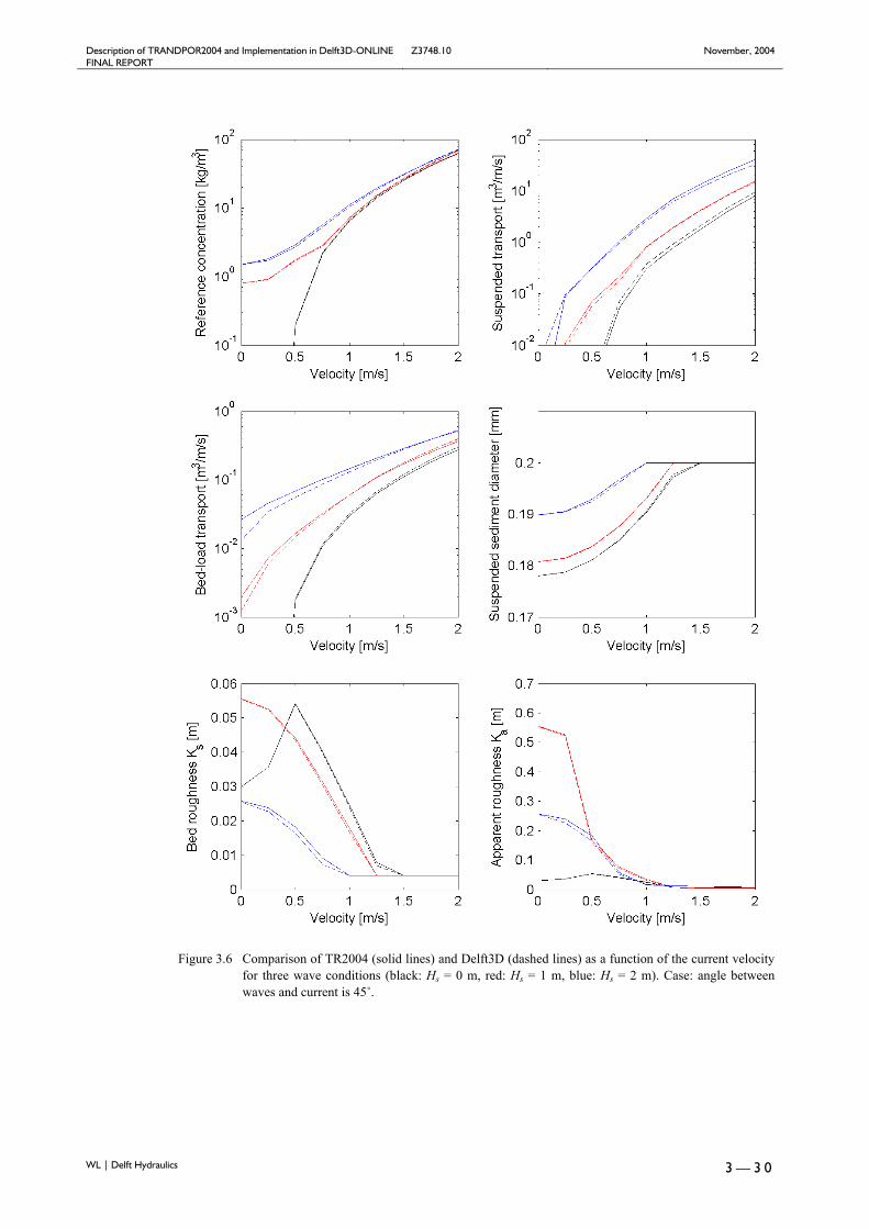
Description of TRANDPOR2004 and Implementation in Delft3D-ONLINE Z3748.10 November, 2004 FINAL REPORT
WL | Delft Hydraulics 3 — 3 0
Figure 3.6 Comparison of TR2004 (solid lines) and Delft3D (dashed lines) as a function of the current velocity
for three wave conditions (black: Hs = 0 m, red: Hs = 1 m, blue: Hs = 2 m). Case: angle between waves and current is 45˚.
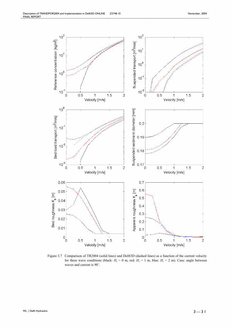
Description of TRANDPOR2004 and Implementation in Delft3D-ONLINE Z3748.10 November, 2004 FINAL REPORT
WL | Delft Hydraulics 3 — 3 1
Figure 3.7 Comparison of TR2004 (solid lines) and Delft3D (dashed lines) as a function of the current velocity
for three wave conditions (black: Hs = 0 m, red: Hs = 1 m, blue: Hs = 2 m). Case: angle between waves and current is 90˚.
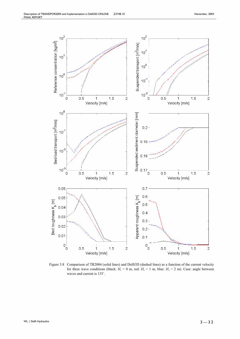
Description of TRANDPOR2004 and Implementation in Delft3D-ONLINE Z3748.10 November, 2004 FINAL REPORT
WL | Delft Hydraulics 3 — 3 2
Figure 3.8 Comparison of TR2004 (solid lines) and Delft3D (dashed lines) as a function of the current velocity
for three wave conditions (black: Hs = 0 m, red: Hs = 1 m, blue: Hs = 2 m). Case: angle between waves and current is 135˚.

Description of TRANDPOR2004 and Implementation in Delft3D-ONLINE Z3748.10 November, 2004 FINAL REPORT
WL | Delft Hydraulics 3 — 3 3
Figure 3.9 Comparison of TR2004 (solid lines) and Delft3D (dashed lines) as a function of the current velocity
for three wave conditions (black: Hs = 0 m, red: Hs = 1 m, blue: Hs = 2 m). Case: angle between waves and current is 180˚ (waves opposing the current).
Description of TRANDPOR2004 and Implementation in Delft3D-ONLINE Z3748.10 November, 2004 FINAL REPORT
WL | Delft Hydraulics 4 — 1
4 Conclusions
In Chapter 2 it was shown that the updated transport formulations of TR2004 performed well in the comparison against over 50 data sets. It was shown that TR2004 was able to give good to reasonable predictions for most datasets for a range of hydrodynamic and sediment conditions. In Chapter 3 a detailed overview is give of the updated formulations in Delft3D-ONLINE. The implementation of TR2004 in Delft3D-ONLINE is part of an update of Delft3D which involves among others as well: the extension of the model to be run in profile mode, inclusion of two breaker delay concepts and the synchronisation of the roughness formulations in the Flow and Transport modules. Furthermore, small inconsistencies in the code were removed. The implementation check for which a detailed comparison between the upgraded Delft3D-model and the TRANSPOR2004 point model was made showed excellent agreement.

Description of TRANDPOR2004 and Implementation in Delft3D-ONLINE Z3748.10 November, 2004 FINAL REPORT
WL | Delft Hydraulics 5 — 1
5 References
Andrews, D.G. and Mcintyre, M.E., 1978: An exact theory of non-linear waves on a Lagrangian-mean flow. J. Fluid Mech., Vol. 89 (4), pp. 609-646.
Davies, A.G. and Villaret, C., 1999. Eulerian drift induced by progressive waves above rippled and very rough bed, p. 1465-1488. Journal of Geophysical Research, Vol. 104, No. C1
Delft Hydraulics, 1999. Voortschrijdend Onderzoek Programma (VOP); Generiek kustonderzoek voor de jaren 2000-2004. Report Z2478, Delft, The Netherlands
Dingemans, M.W., Radder, A.C. and De Vriend, H.J., 1987. Computation of the Driving Forces of Wave-Induced Currents. Coastal Engineering. 11: 539-563.
Forester, C.K., 1979: Higher Order Monotonic Convective Difference Schemes. Journal of Computational Physics, Vol. 23, 1-22.
Fredsøe, J., 1984. Turbulent boundary layer in wave-current interaction. Journal of Hydraulic Engineering, ASCE, Vol. 110, 1103-1120.
Grasmeijer, B.G., 2002. Process-based cross-shore modelling of barred beaches. Doctoral Thesis, Department of Physical Geography, University of Utrecht, Utrecht, The Netherlands
Grasmeijer, B, and Tonnon, P.K., 2003. Preliminary analysis of sand transport measurements at Noordwijk site, North Sea, March-April 2003. Dep. of Physical Geography, University of Utrecht, Utrecht
Grasmeijer, B.T. and Van Rijn, L.C., 1999. Transport of fine sands by currents and waves, Part III: Breaking waves over barred profile with ripples. Journal of Waterway, Port, Coastal and Ocean Engineering, Vol. 125, No. 2
Groeneweg, J. and Klopman, G., 1998. Changes of the mean velocity profiles in the combined wave-current motion in a GLM formulation, J. Fluid Mech., Vol 370, pp. 271-296.
Groeneweg, J., 1999. Wave-current interactions in a generalised Lagrangian Mean formulation, PhD thesis, Delft University of Technology, Delft.
Holthuijsen, L.H., N. Booij and T.H.C. Herbers, 1989. A prediction model for stationary, short-crested waves in shallow water with ambient currents. Coastal Engineering, 13, pp. 23-54.
Holthuijsen, L.H., N. Booij and R.C. Ris, 1993. A spectral wave model for the coastal zone. Proc. of the 2nd Int. Symposium on Ocean Wave Measurement and Analysis, New Orleans, 630-641.
Huang, W. and Spaulding, M., 1996. Modelling horizontal diffusion with sigma coordinate system, Journal of Hydraulic Eng., Vol. 122, No. 6, 349-352.
Isobe, M. and Horikawa, K., 1982. Study on water particle velocities of shoaling and breaking waves. Coastal Engineering in Japan, Vol. 25.
Jonsson , I.G. and Carlsen, N.A., 1976. Experimental and theoretical investigations in an oscillatory rough turbulent boundary layer. Journal of Hydraulic Research, Vol. 14, No. 1, p. 45-60
Jacobs, C. and Dekker, S., 2000. Sediment concentrations due to currents and irregular waves: the effect of grading of the bed material, Measurements Report. Delft University of Technology, Delft, The Netherlands
Kolmogorov, A. N., 1942. Equations of turbulent motion of an incompressible fluid. IZV Akad. Nauk. USSR, Ser. Phys., Vol. 6, pp. 56-58. (translated into English by D.B. Spalding, as Imperial College, Mechanical Engineering Department Report ON/6, 1968, London, U.K.).
Kroon, A., 1994. Sediment transport and morphodynamics of the beach and nearshore zone near Egmond, The Netherlands. Doc. Thesis, Dep. of Physical Geography, Univ. of Utrecht, The Netherlands
Leendertse, J.J., 1987. A three-dimensional alternating direction implicit model with iterative fourth order dissipative non-linear advection terms. WD-333-NETH, The Netherlands Rijkswaterstaat.
Lesser, G., Roelvink, J.A., van Kester, J.A.T.M. and Stelling, G.S., 2004. Development and validation of a three-dimensional morphological model. Journal of Coastal Engineering Vol. 51, pp 883-915.
Madsen, O.S. et al., 1993. Wind stress, bed roughness and sediment suspension on the inner shelf during an extreme storm event. Continental Shelf Research, Vol. 13, No. 11, pp 1303-1324.

Description of TRANDPOR2004 and Implementation in Delft3D-ONLINE Z3748.10 November, 2004 FINAL REPORT
WL | Delft Hydraulics 5 — 2
Mellor, G.L. and A.F. Blumberg, 1985. Modelling vertical and horizontal diffusivities and the sigma coordinate system. Monthly Weather Review, Vol. 113, 1379-1383.
Prandtl, L., 1945. Uber ein neues formelsystem fur die ausgebildete turbulenz (On a new formation for fully developed turbulence). Nachr. Akad. Wiss. (Report of Academy of Sciences) Gottingen, Germany.
Reniers, A.J.H.M., Roelvink, J.A., Thornton, E.B., 2004. Morphodynamic modeling of an embayed beach under wave group forcing. J. Geophys. Res. 109 (C01030).
Rodi, W., 1984. Turbulence models and their application in Hydraulics, State-of-the-art paper article sur l’etat de connaissance. Paper presented by the IAHR-Section on Fundamentals of Division II: Experimental and Mathematical Fluid Dynamics, The Netherlands.
Roelvink, J.A., Meijer, T.J.G.P., Houwman, K., Bakker, R., Spanhoff ,R., 1995. Field validation and application of a coastal profile model. In: Dally, W.R., Zeidler, R.B. (Eds.), Proc. 2nd Int. Conf. on Coastal Dynamics ’95. ASCE, New York, pp. 818–828.
Ruessink, B.G., Walstra, D.J.R. and Southgate, H.N., 2003.Calibration and verification of a parametric wave model on barred beaches. Journal of Coastal Engineering, Vol 48, pp 139-149.
SEDMOC-EU project, 2001. Database sand transport, Delft Hydraulics Simonin, O., R.E. Uittenbogaard, F. Baron, and P.L. Viollet, 1989. Possibilities and limitations to simulate
turbulence fluxes of mass and momentum, measured in a steady stratified mixing layer. In Proc. XXIII IAHR Congress, Ottawa, August 21-25, published by National Research Council Canada, pp. A55-A62.
Sistermans, P.J.G., 2000. Net sediment transport measurements per fraction for well-graded sediment by irregular waves and a current: data report. Delft University of Technology. Delft. The Netherlands
Sistermans, P.J.G., 2002. Graded sediment transport by non-breaking waves and a current. Doc. Thesis. Dep. of Civil Engineering. Delft University of Technology. Delft. The Netherlands
Stelling, G.S., 1983. On the construction of computational methods for shallow water flow problems. Ph.D. Thesis, Delft Univ. of Techn., Delft.
Stelling, G.S. and Kester, van J.A.T.M., 1994. On the approximation of horizontal gradients in sigma coordinates for bathymetry with steep bottom slopes. Int. J. Num. Meth. Fluids, Vol. 18, 915-955.
Stelling, G.S. and Leendertse, J.J., 1991. Approximation of Convective Processes by Cyclic ACI methods. Proceeding 2nd ASCE Conference on Estuarine and Coastal Modelling, Tampa.
Stive, M.J.F. and Wind, H.G., 1986. Cross-shore mean flow in the surf zone. Coastal Eng., 10, pp. 235-340. Svendsen, I.A., 1985. On the formulation of the cross-shore wave-current problem. Proc. Workshop “European
Coastal Zones”. Athens, pp. 1.1-1.9. Soulsby, R.L., L. Hamm, G. Klopman, D. Myrhaug, R.R. Simons, and G.P. Thomas, 1993. Wave-current
interaction within and outside the bottom boundary layer. Coastal Engineering, 21 (1993) 41-69, Elsevier Science Publishers B.V., Amsterdam.
Uittenbogaard, R.E., 1998. Model for eddy diffusivity and viscosity related to sub-grid velocity and bed topography. Note, WL | Delft Hydraulics.
Van Ledden, M., 2003. Sand-mud segregation in estuaries and tidal basins. Doctoral Thesis, Civil Engineering Department, Delft University of Technology , Delft, The Netherlands
Van Rijn, L.C., 1993. Principles of sediment transport in rivers, estuaries and coastal seas. Aqua Publications, The Netherlands
Van Rijn, L.C., 2000. General view on sand transport by currents and waves, Report Z2899.20-Z2099.30-Z2824.30, Delft Hydraulics, Delft, The Netherlands
Van Rijn, L.C., 2002. Approximation formulae for sand transport by currents and waves and implementation in DELFT-MOR. Report Z3054.20, Delft Hydraulics, Delft, The Netherlands.
Van Rijn, L.C., 2003. Sand Transport by currents and waves; general approximation formulae. Coastal Sediments 1999, ASCE, Long Island New York.
Van Rijn, L.C. and Walstra, D.J.R., 2003. Modelling of Sand Transport in Delft3D, WL | Delft Hydraulics report Z3624.
Van Vossen, B., 2000. Horizontal Large Eddy Simulations; evaluation of computations with DELFT3D-FLOW. Report MEAH-197, Delft University of Technology.
Description of TRANDPOR2004 and Implementation in Delft3D-ONLINE Z3748.10 November, 2004 FINAL REPORT
WL | Delft Hydraulics 5 — 3
Verboom, G.K. and Slob, A., 1984. Weakly reflective boundary conditions for two-dimensional water flow problems. 5th Int. Conf. on Finite Elements in Water Resources, June 1984, Vermont. Also Adv. Water Resources, Vol. 7, December 1984, Delft Hydraulics publication No. 322.
Walstra, D.J.R., J.A. Roelvink and J. Groeneweg, 2000: Calculation of wave-driven currents in a 3D mean flow model. In: Coastal Engineering 2000, Billy Edge (ed.), Vol. 2, ASCE, New York, pp. 1050-1063.
Whitehouse, R.J. et al., 1996. Sediment transport measurements at Maplin Sands, Outer Thames Estuary. Report TR 15, HR Wallingford, England
Whitehouse, R.J. et al., 1997. Sediment transport measurements at Boscombe Pier, Poole Bay. Report TR 27, HR Wallingford, England
Wolf, F.C.,J., 1997. Hydrodynamics, sediment transport and daily morphological development of a bar-beach system. Doc. Thesis, Dep. of Physical Geography, Univ. of Utrecht, The Netherlands
Description of TRANDPOR2004 and Implementation in Delft3D-ONLINE Z3748.10 November, 2004 FINAL REPORT
WL | Delft Hydraulics A – 1
A TRANSPOR2004-MODEL; computation of bed forms, bed roughness and sand transport in combined currents and waves
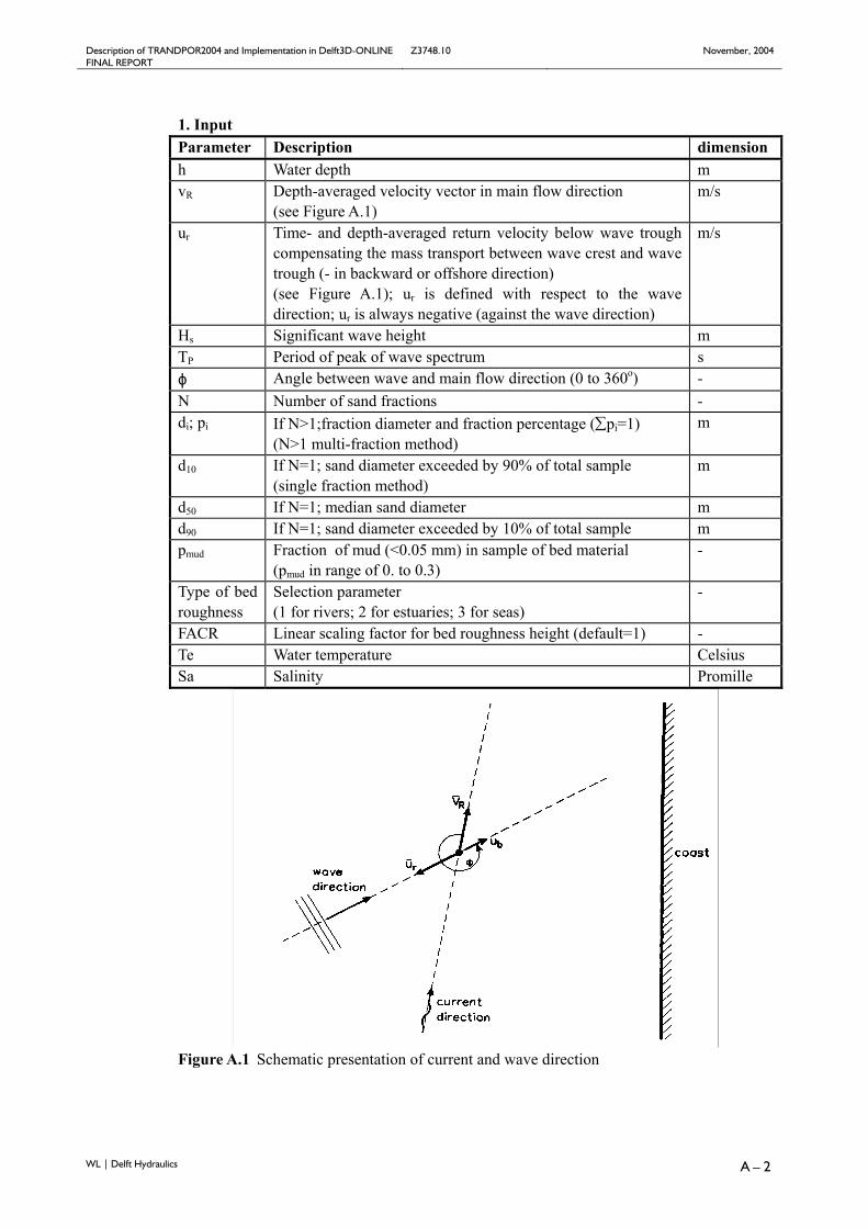
Description of TRANDPOR2004 and Implementation in Delft3D-ONLINE Z3748.10 November, 2004 FINAL REPORT
WL | Delft Hydraulics A – 2
1. Input Parameter Description dimension h Water depth m vR Depth-averaged velocity vector in main flow direction
(see Figure A.1) m/s
ur Time- and depth-averaged return velocity below wave trough compensating the mass transport between wave crest and wave trough (- in backward or offshore direction) (see Figure A.1); ur is defined with respect to the wave direction; ur is always negative (against the wave direction)
m/s
Hs Significant wave height m TP Period of peak of wave spectrum s ϕ Angle between wave and main flow direction (0 to 360o) - N Number of sand fractions - di; pi If N>1;fraction diameter and fraction percentage (∑pi=1)
(N>1 multi-fraction method) m
d10 If N=1; sand diameter exceeded by 90% of total sample (single fraction method)
m
d50 If N=1; median sand diameter m d90 If N=1; sand diameter exceeded by 10% of total sample m pmud Fraction of mud (<0.05 mm) in sample of bed material
(pmud in range of 0. to 0.3) -
Type of bed roughness
Selection parameter (1 for rivers; 2 for estuaries; 3 for seas)
-
FACR Linear scaling factor for bed roughness height (default=1) - Te Water temperature Celsius Sa Salinity Promille
Figure A.1 Schematic presentation of current and wave direction
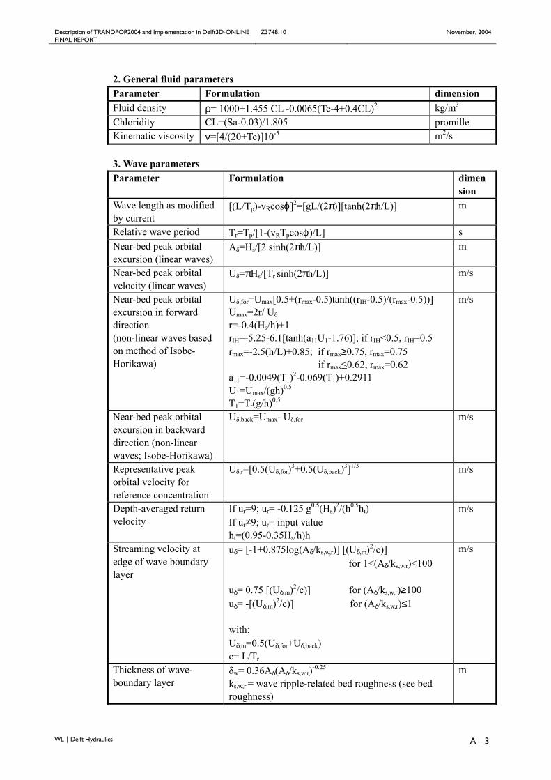
Description of TRANDPOR2004 and Implementation in Delft3D-ONLINE Z3748.10 November, 2004 FINAL REPORT
WL | Delft Hydraulics A – 3
2. General fluid parameters Parameter Formulation dimension Fluid density ρ= 1000+1.455 CL -0.0065(Te-4+0.4CL)2 kg/m3 Chloridity CL=(Sa-0.03)/1.805 promille Kinematic viscosity ν=[4/(20+Te)]10-5 m2/s 3. Wave parameters Parameter Formulation dimen
sion Wave length as modified by current
[(L/Tp)-vRcosϕ]2=[gL/(2π)][tanh(2πh/L)] m
Relative wave period Tr=Tp/[1-(vRTpcosϕ)/L] s Near-bed peak orbital excursion (linear waves)
Aδ=Hs/[2 sinh(2πh/L)] m
Near-bed peak orbital velocity (linear waves)
Uδ=πHs/[Tr sinh(2πh/L)] m/s
Near-bed peak orbital excursion in forward direction (non-linear waves based on method of Isobe-Horikawa)
Uδ,for=Umax[0.5+(rmax-0.5)tanh((rIH-0.5)/(rmax-0.5))] Umax=2r/ Uδ r=-0.4(Hs/h)+1 rIH=-5.25-6.1[tanh(a11U1-1.76)]; if rIH<0.5, rIH=0.5 rmax=-2.5(h/L)+0.85; if rmax≥0.75, rmax=0.75 if rmax≤0.62, rmax=0.62 a11=-0.0049(T1)2-0.069(T1)+0.2911 U1=Umax/(gh)0.5 T1=Tr(g/h)0.5
m/s
Near-bed peak orbital excursion in backward direction (non-linear waves; Isobe-Horikawa)
Uδ,back=Umax- Uδ,for m/s
Representative peak orbital velocity for reference concentration
Uδ,r=[0.5(Uδ,for)3+0.5(Uδ,back)3]1/3 m/s
Depth-averaged return velocity
If ur=9; ur= -0.125 g0.5(Hs)2/(h0.5ht) If ur≠9; ur= input value ht=(0.95-0.35Hs/h)h
m/s
Streaming velocity at edge of wave boundary layer
uδ= [-1+0.875log(Aδ/ks,w,r)] [(Uδ,m)2/c)] for 1<(Aδ/ks,w,r)<100 uδ= 0.75 [(Uδ,m)2/c)] for (Aδ/ks,w,r)≥100 uδ= -[(Uδ,m)2/c)] for (Aδ/ks,w,r)≤1
with: Uδ,m=0.5(Uδ,for+Uδ,back) c= L/Tr
m/s
Thickness of wave-boundary layer
δw= 0.36Aδ(Aδ/ks,w,r)-0.25 ks,w,r = wave ripple-related bed roughness (see bed roughness)
m
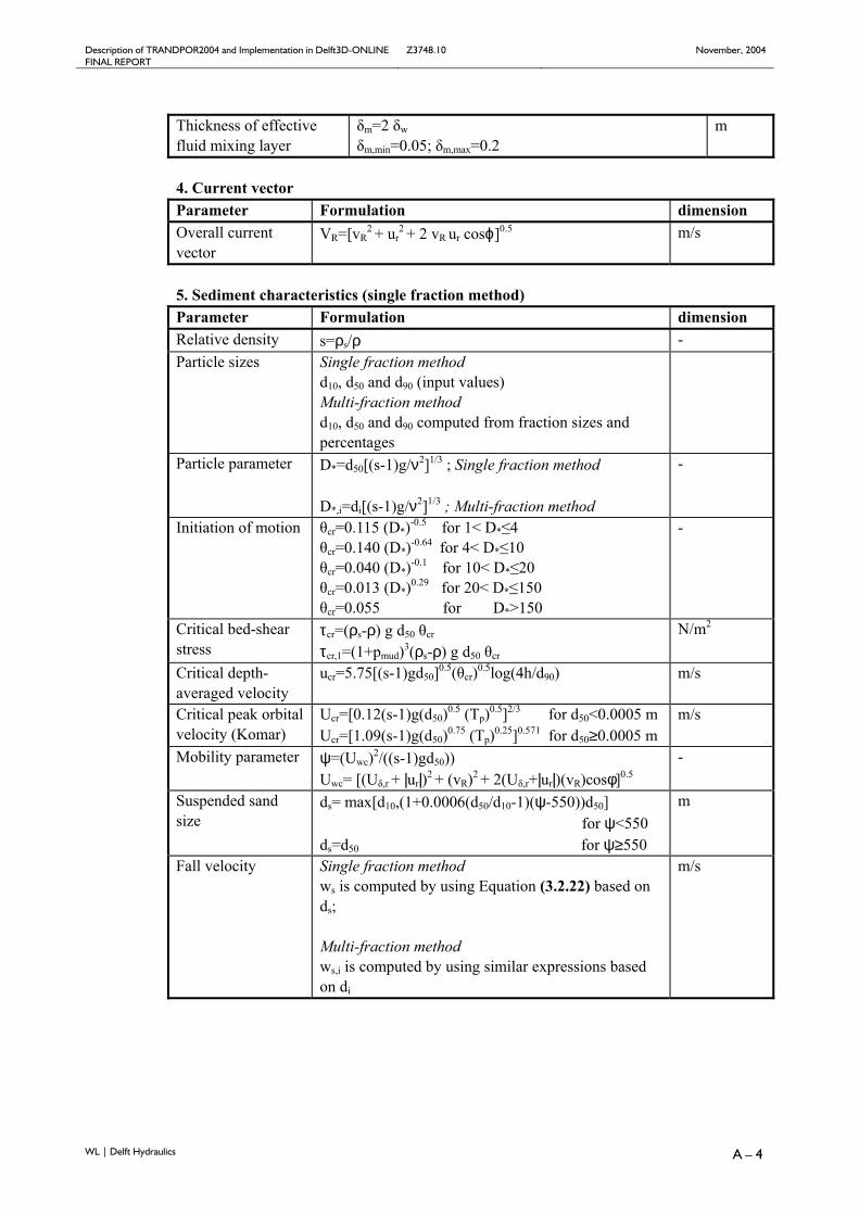
Description of TRANDPOR2004 and Implementation in Delft3D-ONLINE Z3748.10 November, 2004 FINAL REPORT
WL | Delft Hydraulics A – 4
Thickness of effective fluid mixing layer
δm=2 δw δm,min=0.05; δm,max=0.2
m
4. Current vector Parameter Formulation dimension Overall current vector
VR=[vR2 + ur
2 + 2 vR ur cosϕ]0.5 m/s
5. Sediment characteristics (single fraction method) Parameter Formulation dimension Relative density s=ρs/ρ - Particle sizes Single fraction method
d10, d50 and d90 (input values) Multi-fraction method d10, d50 and d90 computed from fraction sizes and percentages
Particle parameter D*=d50[(s-1)g/ν2]1/3 ; Single fraction method D*,i=di[(s-1)g/ν2]1/3 ; Multi-fraction method
-
Initiation of motion θcr=0.115 (D*)-0.5 for 1< D*≤4 θcr=0.140 (D*)-0.64 for 4< D*≤10 θcr=0.040 (D*)-0.1 for 10< D*≤20 θcr=0.013 (D*)0.29 for 20< D*≤150 θcr=0.055 for D*>150
-
Critical bed-shear stress
τcr=(ρs-ρ) g d50 θcr τcr,1=(1+pmud)3(ρs-ρ) g d50 θcr
N/m2
Critical depth-averaged velocity
ucr=5.75[(s-1)gd50]0.5(θcr)0.5log(4h/d90) m/s
Critical peak orbital velocity (Komar)
Ucr=[0.12(s-1)g(d50)0.5 (Tp)0.5]2/3 for d50<0.0005 m Ucr=[1.09(s-1)g(d50)0.75 (Tp)0.25]0.571 for d50≥0.0005 m
m/s
Mobility parameter ψ=(Uwc)2/((s-1)gd50)) Uwc= [(Uδ,r + |ur|)2 + (vR)2 + 2(Uδ,r+|ur|)(vR)cosφ]0.5
-
Suspended sand size
ds= max[d10,(1+0.0006(d50/d10-1)(ψ-550))d50] for ψ<550 ds=d50 for ψ≥550
m
Fall velocity Single fraction method ws is computed by using Equation (3.2.22) based on ds; Multi-fraction method ws,i is computed by using similar expressions based on di
m/s
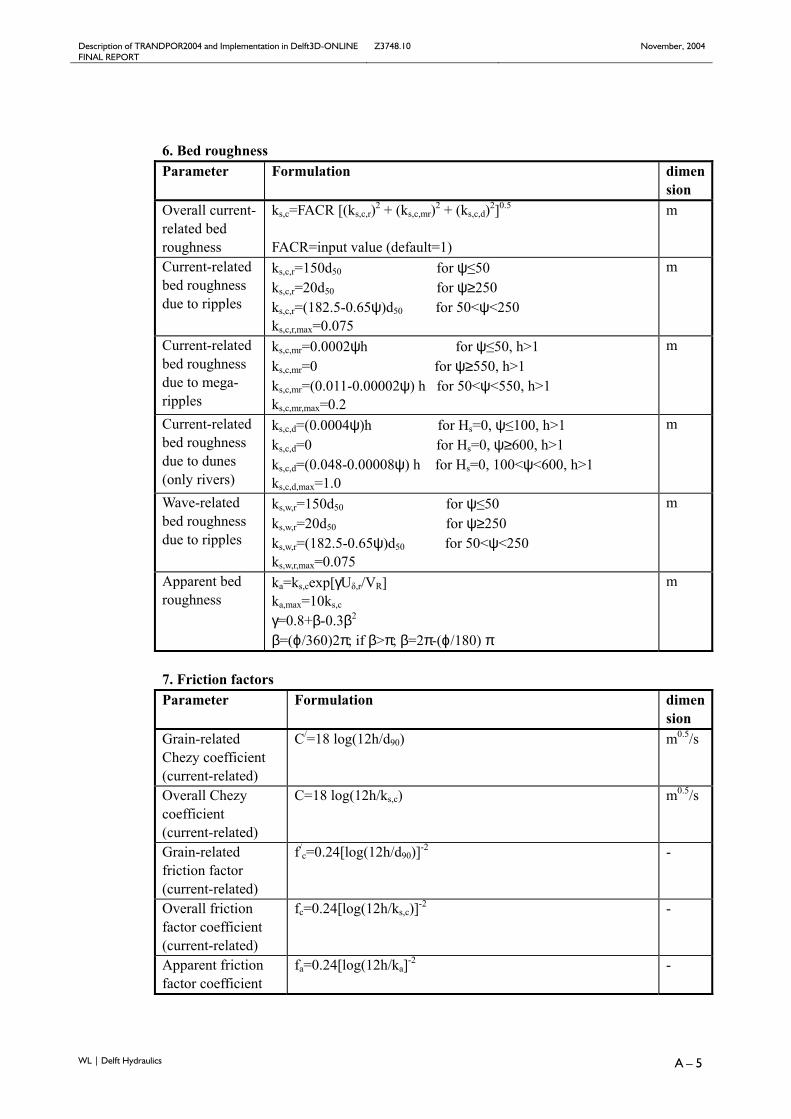
Description of TRANDPOR2004 and Implementation in Delft3D-ONLINE Z3748.10 November, 2004 FINAL REPORT
WL | Delft Hydraulics A – 5
6. Bed roughness Parameter Formulation dimen
sion Overall current-related bed roughness
ks,c=FACR [(ks,c,r)2 + (ks,c,mr)2 + (ks,c,d)2]0.5 FACR=input value (default=1)
m
Current-related bed roughness due to ripples
ks,c,r=150d50 for ψ≤50 ks,c,r=20d50 for ψ≥250 ks,c,r=(182.5-0.65ψ)d50 for 50<ψ<250 ks,c,r,max=0.075
m
Current-related bed roughness due to mega-ripples
ks,c,mr=0.0002ψh for ψ≤50, h>1 ks,c,mr=0 for ψ≥550, h>1 ks,c,mr=(0.011-0.00002ψ) h for 50<ψ<550, h>1 ks,c,mr,max=0.2
m
Current-related bed roughness due to dunes (only rivers)
ks,c,d=(0.0004ψ)h for Hs=0, ψ≤100, h>1 ks,c,d=0 for Hs=0, ψ≥600, h>1 ks,c,d=(0.048-0.00008ψ) h for Hs=0, 100<ψ<600, h>1 ks,c,d,max=1.0
m
Wave-related bed roughness due to ripples
ks,w,r=150d50 for ψ≤50 ks,w,r=20d50 for ψ≥250 ks,w,r=(182.5-0.65ψ)d50 for 50<ψ<250 ks,w,r,max=0.075
m
Apparent bed roughness
ka=ks,cexp[γUδ,r/VR] ka,max=10ks,c
γ=0.8+β-0.3β2 β=(ϕ/360)2π; if β>π; β=2π-(ϕ/180) π
m
7. Friction factors Parameter Formulation dimen
sion Grain-related Chezy coefficient (current-related)
C/=18 log(12h/d90) m0.5/s
Overall Chezy coefficient (current-related)
C=18 log(12h/ks,c) m0.5/s
Grain-related friction factor (current-related)
f/c=0.24[log(12h/d90)]-2 -
Overall friction factor coefficient (current-related)
fc=0.24[log(12h/ks,c)]-2 -
Apparent friction factor coefficient
fa=0.24[log(12h/ka]-2 -
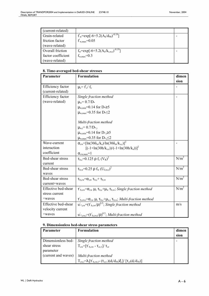
Description of TRANDPOR2004 and Implementation in Delft3D-ONLINE Z3748.10 November, 2004 FINAL REPORT
WL | Delft Hydraulics A – 6
(current-related) Grain-related friction factor (wave-related)
f/w=exp[-6+5.2(Aδ/d90)-0.19]
f/w,max=0.05
-
Overall friction factor coefficient (wave-related)
fw=exp[-6+5.2(Aδ/ks,w,r)-0.19] fw,max=0.3
-
8. Time-averaged bed-shear stresses Parameter Formulation dimen
sion Efficiency factor (current-related)
µc= f/c/ fc -
Efficiency factor (wave-related)
Single fraction method µw= 0.7/D*
µw,min=0.14 for D*≥5 µw,max=0.35 for D*≤2 Multi-fraction method µw,i= 0.7/D*,i µw,min=0.14 for D*,i≥5 µw,max=0.35 for D*,i≤2
-
Wave-current interaction coefficient
αcw=[ln(30δm/ka)/ln(30δm/ks,c)]2 [(-1+ln(30h/ks,c))/(-1+ln(30h/ka))]2 αcw,max=1
-
Bed-shear stress current
τb,c=0.125 ρ fc (VR)2 N/m2
Bed-shear stress waves
τb,w=0.25 ρ fw (Uδ,w,r)2 N/m2
Bed-shear stress current+waves
τb,cw=αcw τb,c+ τb,w N/m2
Effective bed-shear stress current +waves
τ/b,cw=αcw µc τb,c+µw τb,w; Single fraction method
τ/
b,cw,i=αcw µc τb,c+µw,i τb,w; Multi-fraction method
N/m2
Effective bed-shear velocity current +waves
u/*,cw=(τ/
b,cw/ρ)0.5; Single fraction method u/
*,cw,i=(τ/b,cw,i/ρ)0.5; Multi-fraction method
m/s
9. Dimensionless bed-shear stress parameters Parameter Formulation dimen
sion Dimensionless bed-shear stress parameter (current and waves)
Single fraction method Tcw=[τ/
b,cw - τcr,1]/ τcr Multi-fraction method Tcw,i=λi[τ/
b,cw,i- (τcr,1)(di/d50)ξi]/ [τcr(di/d50)]
-
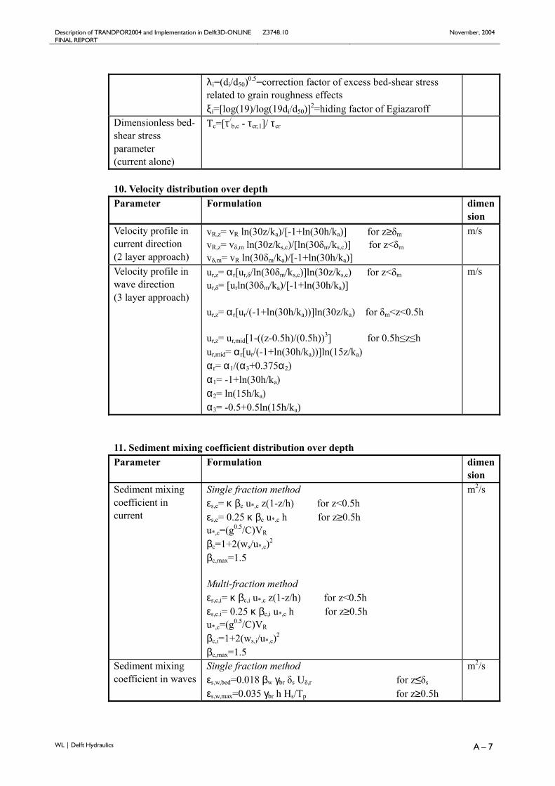
Description of TRANDPOR2004 and Implementation in Delft3D-ONLINE Z3748.10 November, 2004 FINAL REPORT
WL | Delft Hydraulics A – 7
λi=(di/d50)0.5=correction factor of excess bed-shear stress related to grain roughness effects ξi=[log(19)/log(19di/d50)]2=hiding factor of Egiazaroff
Dimensionless bed-shear stress parameter (current alone)
Tc=[τ/b,c - τcr,1]/ τcr
10. Velocity distribution over depth Parameter Formulation dimen
sion Velocity profile in current direction (2 layer approach)
vR,z= vR ln(30z/ka)/[-1+ln(30h/ka)] for z≥δm vR,z= vδ,m ln(30z/ks,c)/[ln(30δm/ks,c)] for z<δm vδ,m= vR ln(30δm/ka)/[-1+ln(30h/ka)]
m/s
Velocity profile in wave direction (3 layer approach)
ur,z= αr[ur,δ/ln(30δm/ks,c)]ln(30z/ks,c) for z<δm ur,δ= [urln(30δm/ka)/[-1+ln(30h/ka)] ur,z= αr[ur/(-1+ln(30h/ka))]ln(30z/ka) for δm<z<0.5h ur,z= ur,mid[1-((z-0.5h)/(0.5h))3] for 0.5h≤z≤h ur,mid= αr[ur/(-1+ln(30h/ka))]ln(15z/ka) αr= α1/(α3+0.375α2) α1= -1+ln(30h/ka) α2= ln(15h/ka) α3= -0.5+0.5ln(15h/ka)
m/s
11. Sediment mixing coefficient distribution over depth Parameter Formulation dimen
sion Sediment mixing coefficient in current
Single fraction method εs,c= κ βc u*,c z(1-z/h) for z<0.5h εs,c= 0.25 κ βc u*,c h for z≥0.5h u*,c=(g0.5/C)VR βc=1+2(ws/u*,c)2 βc,max=1.5 Multi-fraction method εs,c,i= κ βc,i u*,c z(1-z/h) for z<0.5h εs,c.i= 0.25 κ βc,i u*,c h for z≥0.5h u*,c=(g0.5/C)VR βc,i=1+2(ws,i/u*,c)2 βc,max=1.5
m2/s
Sediment mixing coefficient in waves
Single fraction method εs,w,bed=0.018 βw γbr δs Uδ,r for z≤δs εs,w,max=0.035 γbr h Hs/Tp for z≥0.5h
m2/s
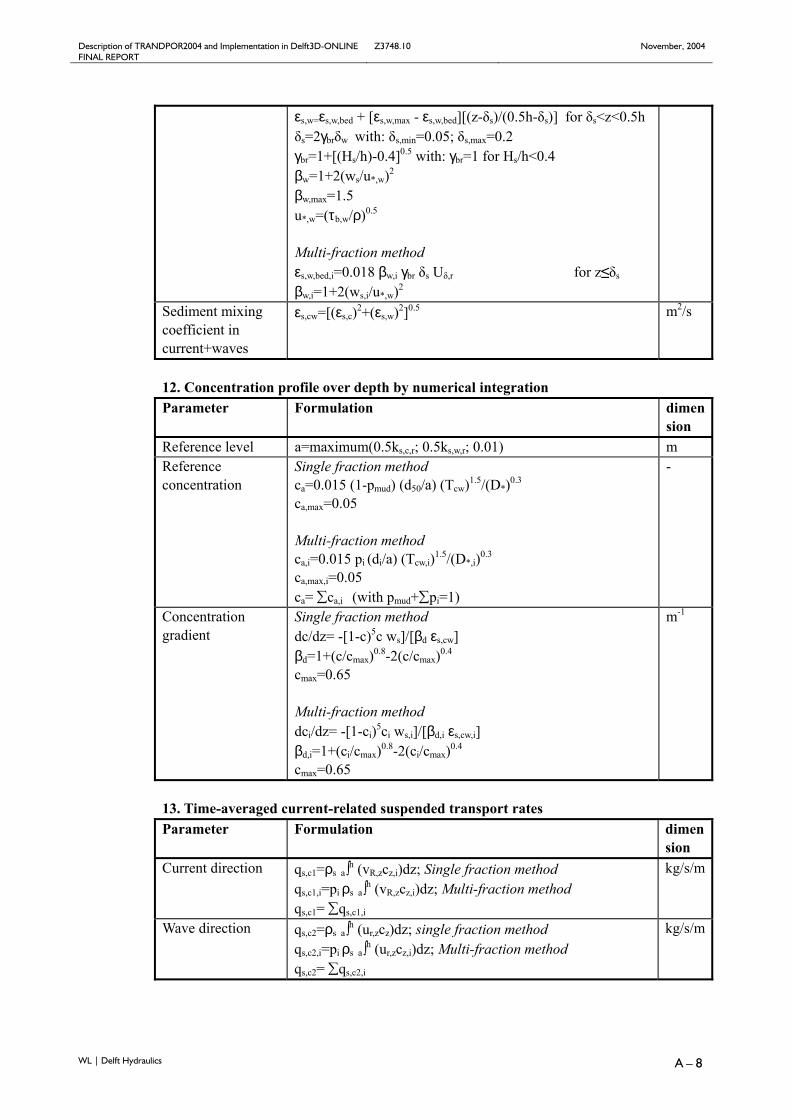
Description of TRANDPOR2004 and Implementation in Delft3D-ONLINE Z3748.10 November, 2004 FINAL REPORT
WL | Delft Hydraulics A – 8
εs,w=εs,w,bed + [εs,w,max - εs,w,bed][(z-δs)/(0.5h-δs)] for δs<z<0.5h δs=2γbrδw with: δs,min=0.05; δs,max=0.2 γbr=1+[(Hs/h)-0.4]0.5 with: γbr=1 for Hs/h<0.4 βw=1+2(ws/u*,w)2 βw,max=1.5 u*,w=(τb,w/ρ)0.5
Multi-fraction method εs,w,bed,i=0.018 βw,i γbr δs Uδ,r for z≤δs βw,i=1+2(ws,i/u*,w)2
Sediment mixing coefficient in current+waves
εs,cw=[(εs,c)2+(εs,w)2]0.5 m2/s
12. Concentration profile over depth by numerical integration Parameter Formulation dimen
sion Reference level a=maximum(0.5ks,c,r; 0.5ks,w,r; 0.01) m Reference concentration
Single fraction method ca=0.015 (1-pmud) (d50/a) (Tcw)1.5/(D*)0.3 ca,max=0.05 Multi-fraction method ca,i=0.015 pi (di/a) (Tcw,i)1.5/(D*,i)0.3 ca,max,i=0.05 ca= ∑ca,i (with pmud+∑pi=1)
-
Concentration gradient
Single fraction method dc/dz= -[1-c)5c ws]/[βd εs,cw] βd=1+(c/cmax)0.8-2(c/cmax)0.4 cmax=0.65 Multi-fraction method dci/dz= -[1-ci)5ci ws,i]/[βd,i εs,cw,i] βd,i=1+(ci/cmax)0.8-2(ci/cmax)0.4 cmax=0.65
m-1
13. Time-averaged current-related suspended transport rates Parameter Formulation dimen
sion Current direction qs,c1=ρs a∫h (vR,zcz,i)dz; Single fraction method
qs,c1,i=pi ρs a∫h (vR,zcz,i)dz; Multi-fraction method qs,c1= ∑qs,c1,i
kg/s/m
Wave direction qs,c2=ρs a∫h (ur,zcz)dz; single fraction method qs,c2,i=pi ρs a∫h (ur,zcz,i)dz; Multi-fraction method qs,c2= ∑qs,c2,i
kg/s/m
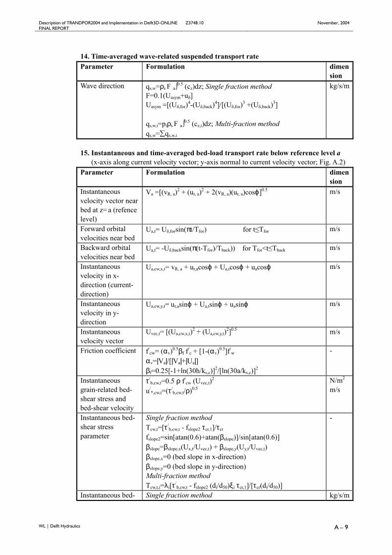
Description of TRANDPOR2004 and Implementation in Delft3D-ONLINE Z3748.10 November, 2004 FINAL REPORT
WL | Delft Hydraulics A – 9
14. Time-averaged wave-related suspended transport rate Parameter Formulation dimen
sion Wave direction qs,w=ρs F a∫0.5 (cz)dz; Single fraction method
F=0.1(Uasym+uδ] Uasym =[(Uδ,for)4-(Uδ,back)4]/[(Uδ,for)3 +(Uδ,back)3] qs,w,i=piρs F a∫0.5 (cz,i)dz; Multi-fraction method qs,w=∑qs,w,i
kg/s/m
15. Instantaneous and time-averaged bed-load transport rate below reference level a (x-axis along current velocity vector; y-axis normal to current velocity vector; Fig. A.2) Parameter Formulation dimen
sion Instantaneous velocity vector near bed at z= a (refence level)
Va =[(vR, a)2 + (ur, a)2 + 2(vR, a)(ur, a)cosϕ]0.5 m/s
Forward orbital velocities near bed
Ua,t= Uδ,forsin(πt/Tfor) for t≤Tfor m/s
Backward orbital velocities near bed
Ua,t= -Uδ,backsin(π(t-Tfor)/Tback)) for Tfor<t≤Tback m/s
Instantaneous velocity in x-direction (current-direction)
Ua,cw,x,t= vR, a + ur,acosϕ + Ua,tcosϕ + uacosϕ m/s
Instantaneous velocity in y-direction
Ua,cw,y,t= ur,asinϕ + Ua,tsinϕ + uasinϕ m/s
Instantaneous velocity vector
Uvec,t= [(Ua,cw,x,t)2 + (Ua,cw,y,t)2]0.5 m/s
Friction coefficient f/cw= (αv)0.5βf f/
c + [1-(αv)0.5]f/w
αv=|Va|/[|Va|+|Ua|] βf=0.25[-1+ln(30h/ks,c)]2/[ln(30a/ks,c)]2
-
Instantaneous grain-related bed-shear stress and bed-shear velocity
τ/b,cw,t=0.5 ρ f/
cw (Uvec,t)2 u/
*,cw,t=(τ/b,cw,t/ρ)0.5
N/m2 m/s
Instantaneous bed-shear stress parameter
Single fraction method Tcw,t=[τ/
b,cw,t - fslope2 τcr,1]/τcr fslope2=sin[atan(0.6)+atan(βslope)]/sin[atan(0.6)] βslope=βslope,x(Ux,t/Uvec,t) + βslope,y(Uy,t/Uvec,t) βslope,x=0 (bed slope in x-direction) βslope,y=0 (bed slope in y-direction) Multi-fraction method Tcw,t,i=λi[τ/
b,cw,t - fslope2 (di/d50)ξi τcr,1]/[τcr(di/d50)]
-
Instantaneous bed- Single fraction method kg/s/m
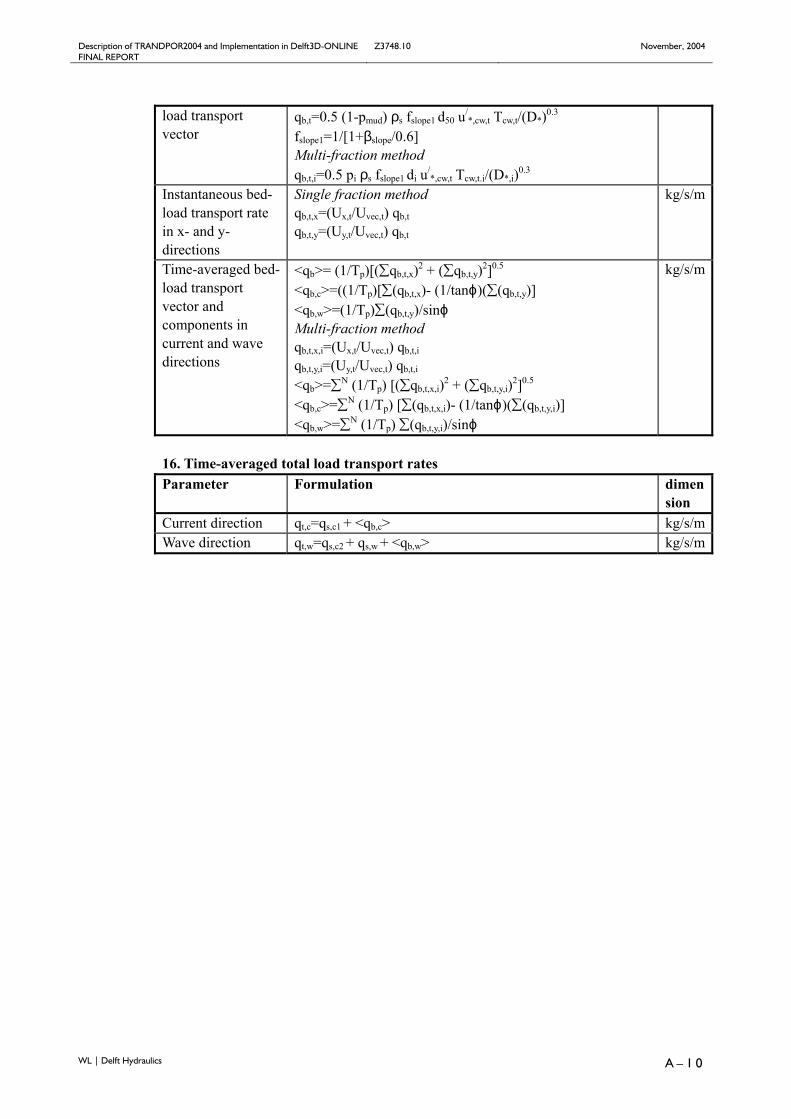
Description of TRANDPOR2004 and Implementation in Delft3D-ONLINE Z3748.10 November, 2004 FINAL REPORT
WL | Delft Hydraulics A – 1 0
load transport vector
qb,t=0.5 (1-pmud) ρs fslope1 d50 u/*,cw,t Tcw,t/(D*)0.3
fslope1=1/[1+βslope/0.6] Multi-fraction method qb,t,i=0.5 pi ρs fslope1 di u/
*,cw,t Tcw,t.i/(D*,i)0.3 Instantaneous bed-load transport rate in x- and y-directions
Single fraction method qb,t,x=(Ux,t/Uvec,t) qb,t qb,t,y=(Uy,t/Uvec,t) qb,t
kg/s/m
Time-averaged bed-load transport vector and components in current and wave directions
<qb>= (1/Tp)[(∑qb,t,x)2 + (∑qb,t,y)2]0.5 <qb,c>=((1/Tp)[∑(qb,t,x)- (1/tanϕ)(∑(qb,t,y)] <qb,w>=(1/Tp)∑(qb,t,y)/sinϕ Multi-fraction method qb,t,x,i=(Ux,t/Uvec,t) qb,t,i qb,t,y,i=(Uy,t/Uvec,t) qb,t,i
<qb>=∑N (1/Tp) [(∑qb,t,x,i)2 + (∑qb,t,y,i)2]0.5 <qb,c>=∑N (1/Tp) [∑(qb,t,x,i)- (1/tanϕ)(∑(qb,t,y,i)] <qb,w>=∑N (1/Tp) ∑(qb,t,y,i)/sinϕ
kg/s/m
16. Time-averaged total load transport rates Parameter Formulation dimen
sion Current direction qt,c=qs,c1 + <qb,c> kg/s/mWave direction qt,w=qs,c2 + qs,w + <qb,w> kg/s/m

Description of TRANDPOR2004 and Implementation in Delft3D-ONLINE Z3748.10 November, 2004 FINAL REPORT
WL | Delft Hydraulics A – 1 1
Figure A.2 Instantaneous velocity vector near bed (at z=a) 17. Bed form dimensions Type of bed forms
Formulation (∆=λ=0 outside validity ranges)
dimen sion
Ripples in rivers
∆r=100d50; if Hs<0.01 and D*<10 and Tc<25 λr=750d50
m
Mega-ripples in rivers
∆mr= 0.02h(10-Tc)(1-e-0.1Tc) if Hs<0.01 and D*<10 and 1≤Tc<10 λmr=0.5h
m
Dunes in rivers
∆d= 0.11h(d50/h)0.3(25-Tc)(1-e-0.5Tc) if Hs<0.01 and 1≤Tc<25 λd=7.3h
m
Sand waves in rivers
∆sw= 0.15h (1-Fr2)(1-e-0.5(Tc-15) ) if Hs<0.01, Tc≥15, Fr<0.8 and h≥1 λsw=10h
m
Ripples in estuaries
∆r=100d50; if Hs<0.01 and D*<10 and Tcw<25 λr=750d50
m
Mega-ripples in restuaries
∆mr= 0.02h(10-Tcw)(1-e-0.1Tcw) if Hs<0.01, D*<10, 1≤Tcw<10 and h≥1 λmr=0.5h
m
Dunes in estuaries
∆d= 0.05h if Hs<0.01 and 1≤Tcw<25 and h≥1 λd=2h
m

Description of TRANDPOR2004 and Implementation in Delft3D-ONLINE Z3748.10 November, 2004 FINAL REPORT
WL | Delft Hydraulics A – 1 2
Sand waves in estuaries
∆sw= 0.05h if Hs<0.01, Tcw≥15, Fr<0.8 and h≥1 λd=3h
m
Ripples in coastal seas
∆r=0.22 Aδ if Hs≥0.01 and ψ<10 λr=5.6∆r ∆r=2.8 10-13 (250-ψ)5 Aδ if Hs≥0.01 and 10≤ψ<250 λr=∆r/[2 10-7(250-ψ)2.5]
m
Mega-ripples in coastal seas
∆mr=0.02 h if Hs≥0.01 and ψ<550 and h≥1 and vR≥0.3 λmr=0.5 h
m
Sand waves in coastal seas
∆sw=0.1 h if Hs≥0.01 and h≥10 and vR≥0.5 λsw=10 h
m