Embed Size (px)
Citation preview

WL | delft hydraulics
Description of TRANSPOR2004 andImplementation in Delft3D-ONLINE
INTERIM REPORT
May 2004
Z3748.00
Report
DG Rijkswaterstaat,
Rijksinstituut voor Kust en Zee | RIKZ
Prepared for:

Prepared for:
DG Rijkswaterstaat,
Rijksinstituut voor Kust en Zee | RIKZ
INTERIM REPORT
L.C. van Rijn and D.J.R. Walstra
Report
Z3748
Description of TRANSPOR2004 andImplementation in Delft3D-ONLINE

Description of TRANDPOR2004 and Implementation in Delft3D-ONLINE Z3748 May, 2004 INTERIM REPORT
WL | Delft Hydraulics i
Contents
1 Introduction..................................................................................................1—12 UPDATED TRANSPOR2004-MODEL......................................................2—1
2.1 Introduction........................................................................................................... 2—1
2.2 Updated sand transport model TRANSPOR2004 (TR2004) .......................... 2—1
2.2.1 Bed roughness predictor............................................................................ 2—1
2.2.2 Predictor for suspended sediment size...................................................... 2—4
2.2.3 Thickness of wave-boundary layer, fluid mixing and sediment mixinglayer ........................................................................................................... 2—4
2.2.4 Wave-induced bed-shear stress ................................................................. 2—5
2.2.5 Wave-induced streaming........................................................................... 2—6
2.2.6 Shields criterion for initiation of motion .................................................. 2—6
2.2.7 Bed-load transport ..................................................................................... 2—7
2.2.8 Wave-related suspended transport ............................................................ 2—8
2.2.9 Near-bed sediment mixing coefficient...................................................... 2—8
2.2.10 Reference concentration and reference level............................................ 2—8
2.2.11 Recalibration ............................................................................................. 2—9
2.3 Intercomparison of transport rates based on TR2004 with TR2000 andTR1993.................................................................................................................2—15
2.4 Application of TR2004-model for graded sediment .......................................2—17
2.4.1 Experiments.............................................................................................2—17
2.4.2 Model results ...........................................................................................2—20
3 Sand transport formulations in DELFT3D model.....................................3—1
3.1 Introduction........................................................................................................... 3—1
3.2 Model description ................................................................................................. 3—2
3.2.1 Hydrodynamics ......................................................................................... 3—2

Description of TRANDPOR2004 and Implementation in Delft3D-ONLINE Z3748 May, 2004 INTERIM REPORT
WL | Delft Hydraulics i i
3.2.2 Waves......................................................................................................... 3—8
3.2.3 Sediment dynamics and bed level evolution ............................................ 3—9
3.2.4 Bed load transport ...................................................................................3—20
3.2.5 Wave-related suspended transport ..........................................................3—22
4 Conclusions...................................................................................................4—1
4.1 Updated sand transport model TRANSPOR2004 (TR2004) ......................... 4—1
4.2 Sand transport formulations in DELFT3D model ........................................... 4—1
5 References.....................................................................................................5—1

Description of TRANDPOR2004 and Implementation in Delft3D-ONLINE Z3748 May, 2004 INTERIM REPORT
WL | Delft Hydraulics 1 — 1
1 Introduction
RIKZ of Rijkswaterstaat and Delft Hydraulics are working together on thedevelopment/improvement, verification/validation and evaluation of morphodynamicmodels within the framework K2005 of Rijkswaterstaat (see Report Z2478 of DelftHydraulics and Website http://vop.wldelft.nl) and within the SANDPIT-project (website:http://sandpit.wldelft.nl).
In 2003 much effort has been spent in the improvement of the DELFT3D-ONLINE modelbased on the engineering sand transport formulations of the TRANSPOR2000 model(TR2000). This work has been described in Delft Hydraulics Report Z3624 by Van Rijn andWalstra (2003). However, the engineering sand transport model TR2000 has recently beenupdated into the TR2004 model within the EU-SANDPIT project. The most importantimprovements involve the refinement of the predictors for the bed roughness and thesuspended sediment size. Up to now these parameters had to be specified by the user of themodels. As a consequence of the use of predictors for bed roughness and suspendedsediment size, it was necessary to recalibrate the reference concentration of the suspendedsediment concentration profile. Given the updated TR2004 model, an effort is necessary tofurther improve the DELFT3D-ONLINE model using the formulations of the updatedTR2004 sand transport model (see Chapter 2). This latter work has been reported in Chapter3.
Chapter 2 addresses the description of the updated TR2004 model and the recalibration ofthe reference concentration using field and laboratory data sets. Furthermore, the results ofthe TR2004 model have been compared with results from older versions (TR1993 andTR2000) of the sand transport model
Chapter 3 addresses the central focus point of the study: the DELFT3D-ONLINE model.The formulations (including the newly derived formulations of the TR2004) implemented inthis 3D-model are described in detail. The implementation of TR2004 in Delft3D-ONLINEis part of an update of Delft3D which involves among others: the extension of the model tobe run in profile mode, an update of the SWAN wave model and the synchronisation of theroughness formulations. The present report only describes the implementation of TR2004formulations in Delft3D-ONLINE. At the end of the project this description will be updatedto completely describe the modifications and improvements in the final updated version ofDelft3D-ONLINE.
Some general conclusions are given in Chapter 4.

Description of TRANDPOR2004 and Implementation in Delft3D-ONLINE Z3748 May, 2004 INTERIM REPORT
WL | Delft Hydraulics 2 — 1
2 UPDATED TRANSPOR2004-MODEL
2.1 Introduction
A new version of the TRANSPOR model has been made (TR2004) based on the results offormer studies, particularly those of 2003 (Van Rijn and Walstra, 2003). The basicformulations of the TR1993-model are described in Appendix A of Van Rijn 1993. Detailedinformation on the Multi-fraction method can be found in Van Rijn (2000).The modifications concern the following points:• Predictor of bed roughness;• Predictor of suspended sediment size• Grain roughness and friction factor;• Wave-induced orbital velocities and streaming near the bed;• Wave-induced bed-shear stress;• Wave-induced sand transport;• Shields criterion for fine sand;• Bed load transport model• Mixing near the bed;• Reference concentration.
In 2003 new bed roughness predictors to simulate the effective roughness of various typesof bed forms were developed and implemented in the latest version of the TRANSPOR-model and in the DELFT3D-model. Experiences so far showed an unrealistic behaviour ofthe roughness predictors of mega-ripples and dunes. Therefore, the predictors of mega-ripple roughness and dune roughness were adjusted slightly resulting in the updatedTR2004-model. The roughness predictor of small-scale ripples in current, waves andcombined current-wave conditions was not changed. In line with this the predictor of thesuspended sediment size was slightly modified.
2.2 Updated sand transport model TRANSPOR2004 (TR2004)
2.2.1 Bed roughness predictor
The TR2004 model includes a bed-roughness predictor for the current-related and wave-related bed roughness parameters. In TR1993 and TR2000 both parameters have to bespecified as user-related input data.
Physical current-related bed roughnessIt is assumed that the physical bed roughness of movable small-scale ripples in naturalconditions is approximately equal to the ripple height: ks,c≅∆r. Furthermore, it is assumed

Description of TRANDPOR2004 and Implementation in Delft3D-ONLINE Z3748 May, 2004 INTERIM REPORT
WL | Delft Hydraulics 2 — 2
that the small-scale ripples are fully developed with a height equal to ∆r=150d50 for ψ≤50 inthe lower wave-current regime and that the ripples disappear with ∆r=0 for ψ≥250 in theupper wave-current regime (sheet flow conditions).
The expressions implemented for small-scale ripples are given by:
( ), , 50
, , 50
, , 50
150 0 50 ( , )
182.5 0.65 50 250 ( , )
20 250 ( )
s c r
s c r
s c r
k d and lower wave current regime SWR ripples
k d and upper wave current regime sheet flow
k d and linear approach in transitional regime
ψ
ψ ψ
ψ
= ≤ ≤ −
= − < < −
= ≥
(2.2.1)
with: ψ= mobility parameter=Uwc2/((s-1)gd50)), (Uwc)
2= (Uδ)2+ vR
2+2(Uw) (vR) |cos ϕ|Uδ= peak orbital velocity near bed= πHs/(Trsinh(2kh)), vR = depth-averaged currentvelocity, ϕ= angle between wave and current motion, Hs= significant wave height,k=2π/L, L= wave length derived from (L/Tp± vR)2=gL tanh(2πh/L)/(2π),Tr= Tp/((1-( vRTp/L)cosϕ)= relative wave period, Tp= peak wave period, h= waterdepth.
Equation (2.2.1) is assumed to be valid for relatively fine sand with d50 in the range of 0.1 to0.5 mm. An estimate of the bed roughness for coarse particles (d50>0.5 mm) can be obtainedby using Equation (2.2.1) for d50=0.5 mm. Thus, d50=0.5 mm for d50≥0.5 mm resulting in amaximum bed roughness height of 0.075 m (upper limit). The lower limit will beks,c=20d50= 0.002 m for sand with d50≤0.1 mm.
When mega-ripples and/or dunes are present on the seabed (if h=water depth>1 m anduc=depth-averaged velocity>0.3 m/s), the physical form roughness (ks,c,mr) of the mega-ripples and dunes should also be taken into account (grain roughness is negligibly small;only form roughness). Compared with the bed roughness predictor implemented earlier(Van Rijn and Walstra, 2003), the expressions of the current-related bed roughness due tomega-ripples and dunes have been refined into:
Mega ripples:
( ), ,
, ,
, ,
, , ,
0.01 0 50 1 0.3
0.011 0.00002 50 550 1 0.3
0 550 1 0.3
0.2
s c mr r
s c mr r
s c mr r
s c mr MAX
k h and and h and v
k h and and h and v
k and and h and v
k
ψ
ψ ψ
ψ
= ≤ ≤ > >
= − < < > >
= ≥ > >
=
(2.2.2)
Dunes (only applicable in rivers, .i.e. no waves):
( ), ,
, ,
, ,
, , ,
0.0004 0 100 1 0.3
0.048 0.0008 100 600 1 0.3
0 600 1 0.3
1.0
s c d r
s c d r
s c d r
s c d MAX
k h and and h and v
k h and and h and v
k and and h and v
k
ψ ψ
ψ ψ
ψ
= ≤ ≤ > >
= − < < > >
= ≥ > >
=
(2.2.3)

Description of TRANDPOR2004 and Implementation in Delft3D-ONLINE Z3748 May, 2004 INTERIM REPORT
WL | Delft Hydraulics 2 — 3
Equation (2.2.2) yields: ks,c,mr=0.01h for ψ=50 and ks,c,mr=0 for ψ=550. Hence, the maximumvalue is ks,c,mr=0.01h. The absolute maximum value of the mega-ripple roughness is assumedto be 0.2 m
Equation (2.2.3) yields: ks,c,d=0 for ψ=0, ks,c,d=0.04h for ψ=100 and ks,c,d=0 for ψ=600.Hence, the maximum value is ks,c,d=0.04 h. The absolute maximum value of the duneroughness is assumed to be 1.0 m.
It is remarked that Equations (2.2.2) and (2.2.3) are slightly different from those presentedin 2003 (see Equations 3.1.10 and 3.1.11 of Van Rijn and Walstra, 2003), because theselatter expressions showed a less realistic behaviour at larger bed-shear stresses. When mega-ripples and/or dunes are present, these values are added to the physical current-related bedroughness of the small-scale ripples by quadratic summation, as follows:
( )0.52 2 2, , , , , , ,s c s c r s c mr s c dk k k k= + + (2.2.4)
The current-related friction coefficient (based on the Darcy-Weisbach approach: f=8g/C2)can be computed as:
2 2
, ,
8 0.24
12 1218log log
c
s c s c
gf
h h
k k
= =
(2.2.5)
Physical wave-related roughness of movable bed ks,w
As regards the physical wave-related bed roughness, only bed forms (ripples) with a lengthscale of the order of the wave orbital diameter near the bed are relevant. Bed forms (mega-ripples, ridges, sand waves) with a length scale much larger than the orbital diameter do notcontribute to the wave-related roughness.The physical wave-related roughness of small-scale ripples is given by:
( )
, , 50
, , 50
, , 50
150 50(lower wave-current regime, SWR ripples)
20 250(upper wave-current regime, sheet flow)
182.5 0.65 50 250(linear approach in transitional regime)
s w r
s w r
s w r
k d for
k d for
k d for
ψ
ψ
ψ ψ
= ≤
= ≥
= − < <
(2.2.6)
with: ψ= mobility parameter=Uwc2/((s-1)gd50)), (Uwc)
2= (Uδ)2+ vR
2+2(Uw) (vR) |cos ϕ|Uδ= peak orbital velocity near bed= πHs/(Trsinh(2kh)), vR = depth-averaged currentvelocity, ϕ= angle between wave and current motion, Hs= significant wave height,k=2π/L, L= wave length derived from (L/Tp± vR)2=gL tanh(2πh/L)/(2π),Tr= Tp/((1-( vRTp/L)cosϕ)= relative wave period, Tp= peak wave period, h= waterdepth.
Equation (2.2.6) includes grain roughness and is assumed to be valid for relatively fine sandwith d50 in the range of 0.1 to 0.5 mm.
The wave-related friction coefficient is computed as:

Description of TRANDPOR2004 and Implementation in Delft3D-ONLINE Z3748 May, 2004 INTERIM REPORT
WL | Delft Hydraulics 2 — 4
0.19
, ,
exp 5.2 6ws w r
Af
kδ
− = −
(2.2.7)
Apparent bed roughness for flow over a movable bedIt is proposed to use the existing expression:
, ,
exp 10a a
s c R s c MAX
k U kand
k v kδγ
= = (2.2.8)
with: Uδ=peak orbital velocity near the bed (see Equation (3.2.15)), vR= depth-averagedcurrent velocity, γ=0.8+ϕ-0.3ϕ2 and ϕ= angle between wave direction and current direction(in radians between 0 and π; 0.5π= 90o, π= 180o). Characteristic γ-values are γ=0.8 for 0,γ=1 for π= 180o and γ=1.63 for 0.5π= 90o. The γ-value is maximum γ=1.63 for ϕ= 0.5π=90o.
Equation (2.2.8) should only be applied to the bed roughness of the small-scale ripplesand mega-ripples.
The current-related apparent friction coefficient (based on the Darcy-Weisbach approach:f=8g/C) can be computed as:
, 2 2
8 0.24
12 1218log log
c a
a a
gf
h h
k k
= =
(2.2.9)
2.2.2 Predictor for suspended sediment size
Compared with the suspended sediment size predictor implemented earlier (Van Rijn andWalstra, 2003), this latter predictor has been refined into:
( )5050, 50
10
50
min 0.5 1 0.0006 1 550 250
250
s
s
dd d d for
d
d d for
ψ ψ
ψ
= + − − < = ≥
(2.2.10)
2.2.3 Thickness of wave-boundary layer, fluid mixing and sediment mixing layer
In TR2004 the wave boundary layer thickness according to (Davies and Villaret, 1999) isused:

Description of TRANDPOR2004 and Implementation in Delft3D-ONLINE Z3748 May, 2004 INTERIM REPORT
WL | Delft Hydraulics 2 — 5
0.25
,, ,
0.36w ws w r
AA
kδ
δδ−
=
(2.2.11)
Aδ= peak orbital excursion at edge of wave boundary layer
Which replaces the wave boundary layer thickness formulation based on that of Jonsson andCarlsen (1976) used in TR1993 and TR2000.
The thickness of the effective fluid mixing layer in TR2004 is modelled as (in metres):
, ,2 0.05 0.2m w m MIN m MAXwith andδ δ δ δ= = = (2.2.12)
The thickness of the effective sediment mixing layer in TR2004 is modelled as:
{ }min 0.5, max 0.05, 2s br wδ γ δ= (2.2.13)
with:
0.5
1 0.4 1 0.4s sbr br
H Hand for
h hγ γ = + − = ≤
(2.2.14)
2.2.4 Wave-induced bed-shear stress
The time-averaged bed-shear stress is computed as:
( )2
, ,
1
4b w w w rf Uδτ ρ= (2.2.15)
with:ρ = fluid densityfw = wave-related friction factor, Eq. (2.2.7)
In TR2004 the peak orbital velocity is refined into:
( ) ( )( )1
3 3 3, , ,0.5 0.5r for backU U Uδ δ δ= + (2.2.16)
Uδ,r = representative peak orbital velocity near the bedUδ,for = peak orbital velocity in forward direction (method of Isobe and Horikawa)Uδ,back= peak orbital velocity in backward direction (method of Isobe and Horikawa)
In TR1993 and TR2000 the Uδ,r-parameter was based on linear wave theory.

Description of TRANDPOR2004 and Implementation in Delft3D-ONLINE Z3748 May, 2004 INTERIM REPORT
WL | Delft Hydraulics 2 — 6
2.2.5 Wave-induced streaming
Based on the results of Van Rijn and Walstra (2003), the wave-induced streaming near thebed can be represented as:
2,
,, , , ,
2, ,
,, ,
2, ,
,, ,
1 0.875log 1 100
0.75 100
1
mm
s w r s w r
m wm
s w r
m wm
s w r
UA Au for
k c k
U Au for
c k
U Au for
c k
δδ δδ
δ δδ
δ δδ
= − + < <
= ≥
= − ≤
(2.2.17)
with:uδ,m= streaming velocity at edge of wave boundary layer,Uδ,m=0.5(Uδ,for+Uδ,back)= peak orbital velocity at edge of wave boundary layer,c= wave propagation velocity,Aδ= peak orbital excursion at edge of wave boundary layer=TpUδ/(2π),Tp= peak wave period,ks,w,r= wave-related bed roughness
In TR2004 the streaming velocity vector is added to the current-related velocity vector atlevel z=δ.
2.2.6 Shields criterion for initiation of motion
In TR2004 the critical bed-shear stress for initiation of motion is modelled as:
( )3
, , ,1b cr mud b cr opτ τ= + (2.2.18)
τb,cr,o= critical bed-shear stress for pure sand (no mud)pmud= fraction (0 to 0.3) of mud (Van Ledden, 2003)
In TR1993 and TR2000 the dimensionless Shields criterion for initiation of motion of veryfine sediments is represented as:
**
0.244cr for D
DΘ = ≤ (2.2.19)
with Θcr=τb,cr,o/((s-1)gd50 and D*=d50[(s-1)g/ν2]1/3, s= ρs/ρ= relative density, ν=kinematicviscosity coefficient.
A better representation based on experimental data is given by (See Van Rijn, 1993):
0.5* *0.115 4cr D for D−Θ = ≤ (2.2.20)

Description of TRANDPOR2004 and Implementation in Delft3D-ONLINE Z3748 May, 2004 INTERIM REPORT
WL | Delft Hydraulics 2 — 7
which is implemented in TR2004.
2.2.7 Bed-load transport
Bed load transport modelThe net bed-load transport rate in conditions with uniform bed material is obtained by time-averaging (over the wave period T) of the instantaneous transport rate using the bed-loadtransport model (quasi-steady approach), as follows:
,
1b b tq q dt
T = ∫ (2.2.21)
with qb,t = F(instantaneous hydrodynamic and sediment transport parameters).
The formula applied, reads as:
0.5' ', , , , ,0.3
50 *,
0.5 b cw t b cw t b crb s
b cr
q d Dτ τ τ
ρρ τ
− −=
(2.2.22)
in which:τ/b,cw,t = instantaneous grain-related bed-shear stress due to both current and wave motion =
0.5 ρ f/cw (Uδ,cw,t)
2,Uδ,cw,t = instantaneous velocity due to current and wave motion at edge of wave boundary
layer,f/
c = current-related grain friction coefficient =0.24(log(12h/ks,grain))-2,
f/w = wave-related grain friction coefficient=Exp[-6+5.2(Aδ,w/ks,grain)
-0.19],
α = coefficient related to relative strength of wave and current motion:ˆ
R
U
vδα = ,
Uδ = the peak orbital velocity, vR is the depth averaged current,
βf = coefficient related to vertical structure of velocity profile,Aδ = peak orbital excursion,τb,cr = critical bed-shear stress according to Shields,ρs = sediment density,ρ = fluid density,d50 = particle size,D* = dimensionless particle size.
The two most influential parameters of Eq. (2.2.22) are: 'cwf and ks,grain.
Various field data sets from the literature and new data sets (laboratory and field) collectedwithin the SANDPIT project have been used to verify/improve these parameters of the bed-load transport formulations (see Van Rijn and Walstra, 2003).
In TR2000, these two parameters ( 'cwf and ks,grain) are modelled as:

Description of TRANDPOR2004 and Implementation in Delft3D-ONLINE Z3748 May, 2004 INTERIM REPORT
WL | Delft Hydraulics 2 — 8
( )' ' '1cw f c wf f fαβ α= + − (2.2.23)
, 90 1 3s grain grain graink d with between andα α= (2.2.24)
Based on the findings of Van Rijn and Walstra (2003), the following expressions havebeen implemented in TR2004:
( )' 0.5 ' 0.5 '1cw f c wf f fα β α= + − (2.2.25)
, 90s graink d= (2.2.26)
2.2.8 Wave-related suspended transport
The wave-related suspended transport component is modelled as follows:
4 4, ,
, ,3 3, ,
for backs w m
for back
U Uq u cdz
U Uδ δ
δδ δ
γ −
= + + ∫ (2.2.27)
with: Uδ,for= near-bed peak orbital velocity in onshore direction (in wave direction) andUδ,back= near-bed peak orbital velocity in offshore direction (against wave direction),uδ,m= wave-induced streaming velocity near the bed, c= time-averaged concentrationand γ= phase lag function.
In TR2004 (based on the findings of Van Rijn and Walstra, 2003), the phase lag functionis: γ= 0.1 in stead of γ= 0.2 as was used in TR2000.
2.2.9 Near-bed sediment mixing coefficient
The mixing coefficient near the bed is modelled as:
, ,0.018w bed w s rUδε β δ= (2.2.28)
with Uδ,r according to Equation (2.2.16) and δs according to Equation (2.2.13).
2.2.10 Reference concentration and reference level
The reference level in TR2004 is described by:
( ), , , ,max 0.5 ,0.5 ,0.01s c r s w ra k k= (2.2.29)
with ks,c,r= current-related bed roughness height due to small-scale ripples and ks,w,r= wave-related bed roughness height due to small-scale ripples.Similarly as in TR1993 and TR2000, the reference concentration (single fraction approach)in TR2004 is described by:

Description of TRANDPOR2004 and Implementation in Delft3D-ONLINE Z3748 May, 2004 INTERIM REPORT
WL | Delft Hydraulics 2 — 9
( )( )
1.5
50
s ,0.30.015 0.05a
a a MAX s
d Tc with c
a Dρ ρ
∗
= = (2.2.30)
2.2.11 Recalibration
The T-parameter of Equation (2.2.30) involves the computation of the wave-related bed-shear stress and a wave-related efficiency factor µw. This latter parameter has beenrecalibrated using a dataset of 53 cases (see Table 3.2.1) from combined quasi-steady andoscillatory flow cases, resulting in:
( )
*
( ), *
( ), *
0.7
0.35 2
0.14 5
w
w MAX
w MIN
D
for D
for D
µ
µ
µ
=
= <
= >
!
!
!
(2.2.31)
with D*= particle size parameter,
The measured concentration in the lowest measuring point above the bed (in the range of0.015 m for laboratory cases to 0.5 m for field cases) has been used as measured referenceconcentration. To better understand the variability within the available dataset, someconcentration profiles measured under similar conditions are presented in Figures 2.2.1Aand 2.2.1B, showing differences in the range of a factor 5 to 10.
Figure 2.2.2 shows measured and computed reference concentrations for 53 datasets.Variation ranges of a factor of 2 are also indicated. About 75% of the computed referenceconcentrations are within a factor of 2 of the measured concentrations.
Figure 2.2.3 shows measured and computed suspended sand transport rates between thelowest and highest measurement points for 34 datasets. Measured transport rates were notavailable for the Delta flume cases (wave-alone cases) and the Noordwijk Spring 2003 fieldcases. Variation ranges of a factor of 2 are also indicated. About 65% of the computedsuspended transport rates (34 cases) are within a factor of 2 of the measured values.
Figures 2.2.4 to 2.2.21 show various computed and measured concentration profiles basedon the recalibrated TR2004 model.

Description of TRANDPOR2004 and Implementation in Delft3D-ONLINE Z3748 May, 2004 INTERIM REPORT
WL | Delft Hydraulics 2 — 1 0
Site Sedimentsized50(mm)
Waterdepthrange(m)
Waveheightrange(m)
Flowvelocityrange
(m/s)
Reference
Boscombe1977-1978
0.25 4.8-5.3 0.45-1.05 0.2-0.4 Whitehouse et al., 1997
Maplin sands1973-1975
0.14 2.8-3.2 0.4-0.9 0.07-0.34 Whitehouse et al., 1996
Egmond1989-1990
0.3-0.35 1-1.6 0.2-0.9 0.06-0.55 Kroon, 1994Wolf, 1997
Egmond 1998 0.25 2.5-3.1 0.45-1.1 0.1-0.3 Grasmeijer, 2002Noordwijkspring 2003
0.22 13-15 2.2-2.8 0.1-0.5 Grasmeijer and Tonnon,2003
Duck 1991 0.15 13 3.75 0.4-0.6 Madsen et al., 1993Deltaflume1987
0.21 1.1-2.1 0.3-1.1 0 SEDMOC sand transportdatabase, 2001
Deltaflume1997
0.16-0.33 4.5 1-1.5 0 SEDMOC sand transportdatabase, 2001
DH Vinje lab.basin
0.1 0.4 0.1-0.14 0.13-0.32 SEDMOC sand transportdatabase, 2001
TUD flume 0.2 0.5 0.12-0.15 0.1-0.45 SEDMOC sand transportdatabase, 2001
Table 2.2.1 Summary of field and laboratory datasets used for calibration of referenceconcentration of TR2004 sand transport model
0
0.2
0.4
0.6
0.8
1
1.2
1.4
1.6
1.8
2
0.01 0.1 1 10
Concentration (kg/m3)
Hei
ghtab
ove
bed
(m
EGMONDBEACH, h=2.1 m, Hs=1.1 m, Tp=7.2 s, V=0.3 m/s, d50=0.25 mm
DELTAFLUME, h=2.0 m, Hs=1.1 m, Tp=5.8 s, V= 0 m/s, d50=0.21 mm
Figure 2.2.1A Comparison of concentration profiles measured under similar conditionsin water depth of about 2 m (d50 in range of 0.2 to 0.25 mm)

Description of TRANDPOR2004 and Implementation in Delft3D-ONLINE Z3748 May, 2004 INTERIM REPORT
WL | Delft Hydraulics 2 — 1 1
0
0.2
0.4
0.6
0.8
1
1.2
1.4
1.6
1.8
2
0.001 0.01 0.1 1
Concentration (kg/m3)
Hei
gh
tab
ove
bed
(m
Maplin Sands M24-03; d50=0.14 mm, h=3.2 m, Hs=0.73 m, v=0.083 m/s
Maplin Sands M22-01; d50=0.14 mm, h=3.2 m, Hs=0.68 m, v=0.1 m/s
Figure 2.2.1B Comparison of concentration profiles measured under similar conditionsin water depth of about 3 m (d50 of about 0.14 mm)
0.01
0.1
1
10
100
0.01 0.1 1 10 100
Ca,computed (kg/m3)
Ca,
mea
sure
d(k
g/m
3
Line of perfect agreementVariation range of factor 2Egmond 1998, d50=0.25 mmBoscombe Pier 1977-1978, d50=0.25 mmDeltaflume 1997, d50=0.16-0.33 mmDeltaflume 1987, d50=0.21 mmEgmond 1989-1990, d50=0.3-0.35 mmVinje Lab. basin, d50=0.1 mmTUDLab. basin, d50=0.2 mmMaplin Sands 1973-1975, d50=0.14 mmNoordwijk 2003, d50=0.22 mmDuck 1991, d50=0.15 mm
Figure 2.2.2 Measured and computed reference concentrations

Description of TRANDPOR2004 and Implementation in Delft3D-ONLINE Z3748 May, 2004 INTERIM REPORT
WL | Delft Hydraulics 2 — 1 2
0.0001
0.001
0.01
0.1
1
0.0001 0.001 0.01 0.1 1
qs,computed (kg/s/m)
qs,
mea
sure
d(k
g/s
/m)
Line of perfect agreementEgmond 89-90Vinje BasinTUDflumevariation range of factor 2Egmond 98Boscombe 77-78Maplin 73-75
Figure 2.2.3 Measured and computed suspended sand transport rates
0
0.1
0.2
0.3
0.4
0.5
0.6
0.7
0.8
0.9
1
0.00001 0.0001 0.001 0.01 0.1 1 10
Concentration (kg/m3)
Rel
ativ
eh
eig
ht
abo
veb
ed(z
/h
Hs=1 m, v=0.3 m/s
Computed Group 4
Figure 2.2.4 Boscombe Pier 1977-1978
0
0.1
0.2
0.3
0.4
0.5
0.6
0.7
0.8
0.9
1
0.00001 0.0001 0.001 0.01 0.1 1
Concentration (kg/m3)
Rel
ativ
eh
eig
ht
abo
veb
ed(z
/h
Hs=0.5 m, v=0.2 m/s
Computed group 1
Figure 2.2.5 Boscombe Pier 1977-1978

Description of TRANDPOR2004 and Implementation in Delft3D-ONLINE Z3748 May, 2004 INTERIM REPORT
WL | Delft Hydraulics 2 — 1 3
0
0.1
0.2
0.3
0.4
0.5
0.6
0.7
0.8
0.9
1
0.0001 0.001 0.01 0.1 1 10Concentration (kg/m3)
Rel
.h
eig
ht
abo
veb
ed(z
/h
Measured 3C
Measured 3C
Computed 3C
Figure 2.2.6 Egmond 1989-1990
0
0.1
0.2
0.3
0.4
0.5
0.6
0.7
0.8
0.9
1
0.001 0.01 0.1 1 10Concentration (kg/m3)
Rel
.hei
ghtab
ove
bed
(z/h
Measured 4AMeasured 4AMeasured 4AComputed 4A
Figure 2.2.7 Egmond 1989-1990
0
0.1
0.2
0.3
0.4
0.5
0.6
0.7
0.8
0.9
1
0.0001 0.001 0.01 0.1 1 10Concentration (kg/m3)
Rel
.hei
ghtab
ove
bed
(z/h
Measured Class4
Computed
Figure 2.2.8 Egmond 1998
0
0.1
0.2
0.3
0.4
0.5
0.6
0.7
0.8
0.9
1
0.0001 0.001 0.01 0.1 1 10Concentration (kg/m3)
Rel
.hei
ghtab
ove
bed
(z/h
Measured Class6
Computed
Figure 2.2.9 Egmond 1998
0
0.1
0.2
0.3
0.4
0.5
0.6
0.7
0.8
0.9
1
0.0001 0.001 0.01 0.1 1Concentration (kg/m3)
Rel
.h
eig
ht
abo
veb
ed(z
/h
Measured 2206-2207
Computed
Figure 2.2.10 Noordwijk Spring 2003
0
0.1
0.2
0.3
0.4
0.5
0.6
0.7
0.8
0.9
1
0.0001 0.001 0.01 0.1 1 10Concentration (kg/m3)
Rel
.hei
ghtab
ove
bed
(z/h
Measured 2209
Computed
Figure 2.2.11 Noordwijk Spring 2003

Description of TRANDPOR2004 and Implementation in Delft3D-ONLINE Z3748 May, 2004 INTERIM REPORT
WL | Delft Hydraulics 2 — 1 4
0
0.1
0.2
0.3
0.4
0.5
0.6
0.7
0.8
0.9
1
0.1 1 10Concentration (kg/m3)
Rel
.hei
gh
tab
ove
bed
(z/h
Computed 2HComputed 2IMeasured 2HMeasured 2I
Figure 2.2.12 Deltaflume 1987
0
0.1
0.2
0.3
0.4
0.5
0.6
0.7
0.8
0.9
1
0.001 0.01 0.1 1 10
Concentration (kg/m3)
Rel
.hei
gh
tab
ove
bed
(z/h
measured Hs/h=0.19 (2C)measured Hs/h=0.55 (2F)Computed 2CComputed 2F
Figure 2.2.13 Deltaflume 1987
0
0.1
0.2
0.3
0.4
0.5
0.6
0.7
0.8
0.9
1
0.01 0.1 1 10
Concentration (kg/m3)
Rel
.hei
gh
tab
ove
bed
(z/h
measured Hs= 1 m (Hs/h=0.22), case 1Ameasured Hs= 1.25 m (Hs/h=0.27), case 1BComputed 1AComputed 1B
Figure 2.2.14 Deltaflume 1997
0
0.1
0.2
0.3
0.4
0.5
0.6
0.7
0.8
0.9
1
0.01 0.1 1 10
Concentration (kg/m3)
Rel
.hei
gh
tab
ove
bed
(z/h
measured Hs= 1 m (Hs/h=0.22; 1C)measured Hs= 1.25 m (Hs/h=0.27; 1D)measured Hs= 1.5 m (Hs/h=0.33; 1E)Computed 1CComputed 1DComputed 1E
Figure 2.2.15 Deltaflume 1997
0
0.1
0.2
0.3
0.4
0.5
0.6
0.7
0.8
0.9
1
0.01 0.1 1 10
Concentration (kg/m3)
Rel
.hei
gh
tab
ove
bed
(z/h
Measured Hs=0.105 m, v=0.245 m/s
Computed
Figure 2.2.16 DH Vinje Laboratory basin
0
0.1
0.2
0.3
0.4
0.5
0.6
0.7
0.8
0.9
1
0.01 0.1 1 10
Concentration (kg/m3)
Rel
.hei
gh
tab
ove
bed
(z/h
Measured Hs=0.137 m, v=0.317 m/s
Computed
Figure 2.2.17 DH Vinje Laboratory basin

Description of TRANDPOR2004 and Implementation in Delft3D-ONLINE Z3748 May, 2004 INTERIM REPORT
WL | Delft Hydraulics 2 — 1 5
0
0.1
0.2
0.3
0.4
0.5
0.6
0.7
0.8
0.9
1
0.01 0.1 1 10
Concentration (kg/m3)
Rel
.hei
gh
tab
ove
bed
(z/h
Measured Hs=0.133 m, v=0.13 m/sComputed
Figure 2.2.18 DH Vinje Laboratory Basin
0
0.1
0.2
0.3
0.4
0.5
0.6
0.7
0.8
0.9
1
0.00001 0.0001 0.001 0.01 0.1 1
Concentration (kg/m3)
Rel
.hei
gh
tab
ove
bed
(z/h
Measured Hs=0.123 m, v=0.22 m/sComputed
Figure 2.2.19 TUD Flume
0
0.1
0.2
0.3
0.4
0.5
0.6
0.7
0.8
0.9
1
0.0001 0.001 0.01 0.1 1 10
Concentration (kg/m3)
Rel
.hei
gh
tab
ove
bed
(z/h
Measured Hs=0.119 m/s, v=0.44 m/sComputed
Figure 2.2.20 TUD Flume
0
0.1
0.2
0.3
0.4
0.5
0.6
0.7
0.8
0.9
1
0.01 0.1 1 10Concentration (kg/m3)
Rel
ativ
eh
eig
ht
abo
veb
ed(z
/hMeasured Duck Shelf 1991 (h=13 m)Computed
Figure 2.2.21 DUCK 1991
2.3 Intercomparison of transport rates based on TR2004 with TR2000 and TR1993
Figures 2.3.1 and 2.3.2 show intercomparison-results of the TR2004-model with TR2000-and TR1993-models based on reference case computations for a water depth of h=5 m and amedian particle size of d50= 0.25 mm (see Appendix A of Van Rijn, 1993).The significant wave height varies between 0 and 3 m; the depth-averaged current velocityvaries between 0.1 and 2 m/s. The wave-current angle is 90 degrees. Other parameters are:d90= 0.5 mm, water temperature= 15 oCelsius and salinity= 30 promille.The TR2004-model results (total sand transport rates) are based on predicted bed roughnessand suspended sediment size values, whereas the TR-2000 and TR1993-model results arebased on prescribed values in the range of ks=0.02 to 0.1 m and ds= 0.17 to 0.25 mm (seeVan Rijn, 1993). Measured transport rates (mainly suspended sand transport; see Van Rijn,2000) for the current-alone cases (no waves) are also shown in Figures 2.3.1 and 2.3.2.

Description of TRANDPOR2004 and Implementation in Delft3D-ONLINE Z3748 May, 2004 INTERIM REPORT
WL | Delft Hydraulics 2 — 1 6
Figure 2.3.1 shows that the TR2004 results are considerably smaller than those of theTR2000-model for wave heights of Hs=0.5 and 1 m. This effect is caused by a lesspronounced effect of the bed roughness on the sand transport rate in the TR2004-model. Theresults of the TR2004 and TR2000 models are in reasonably good agreement for waveheights of Hs= 2 and 3 m.
0.001
0.01
0.1
1
10
100
0 0.2 0.4 0.6 0.8 1 1.2 1.4 1.6 1.8 2 2.2
Depth-averaged current velocity (m/s)
To
tal
curr
ent-
rela
ted
san
dtr
ansp
ort
(kg
/s/m
TRANSPOR2000
TRANSPOR2004
Eastern and Western Scheldt data (Netherlands)
Nile river data (Egypt)
Mississippi river data (USA)Hs=0
Hs=0.5
h = 5 md50=0.25 mmd90=0.50 mm
Hs=1 m
Hs=2 m
Hs=3 m
Figure 2.3.1 Intercomparison of TR2004 and TR2000 model results for constantwater depth of 5 m and particle size of 0.25 mm
The TR2004-model yields smaller transport rates for current-alone cases (no waves),particularly for current-velocities larger than 1.4 m/s. This latter effect is also caused by themodelling of the bed roughness; the TR2004-model yields smaller values in the upperregime. The TR2004 results are in good agreement with the measured data points (current-alone cases), whereas the TR2004-model seems to over predict the measured transport rates(bed-load transport is assumed to negligibly small).
Figure 2.3.2 shows that the TR2004 results are quite close to the TR1993 results for waveheights of Hs= 1, 2 and 3 m. The TR2004 model yields smaller transport rates for the waveheights of Hs=0.5 and Hs=0 m (current-alone case), particularly for current velocities largerthan 1.4 m/s. This latter effect is caused by smaller bed roughness values in the upperregime using the TR2004-model.. The TR2004 results are in good agreement with themeasured data points (current-alone cases), whereas the TR1993-model seems to overpredict the measured transport rates (bed-load transport is assumed to negligibly small).

Description of TRANDPOR2004 and Implementation in Delft3D-ONLINE Z3748 May, 2004 INTERIM REPORT
WL | Delft Hydraulics 2 — 1 7
0.001
0.01
0.1
1
10
100
0 0.2 0.4 0.6 0.8 1 1.2 1.4 1.6 1.8 2 2.2
Depth-averaged current velocity (m/s)
To
tal
curr
ent-
rela
ted
san
dtr
ansp
ort
(kg
/s/m
TRANSPOR1993TRANSPOR2004Eastern and Western Scheldt data (Netherlands)
Nile river data (Egypt)Mississippi river data (USA)Hs=0
Hs=0.5
h = 5 md50=0.25 mmd90=0.50 mm
Hs=1 m
Hs=2 m
Hs=3 m
Figure 2.3.2 Intercomparison of TR2004 and TR1993 model results for constantwater depth of 5 m and particle size of 0.25 mm
2.4 Application of TR2004-model for graded sediment
2.4.1 Experiments
Experiments over a horizontal sand bed have been carried out in a small-scale wave-currentflume of the Fluids Mechanics Laboratory of the Delft University of Technology (Jacobsand Dekker, 2000 and Sistermans, 2000). Two types of sand have been used in theexperimental program: uniform sand with d50 of about 0.16 mm and graded sand with d50 ofabout 0.25 mm. The water depth was about 0.5 m in all tests. The hydrodynamic conditionsare: irregular waves superimposed on a following current. The significant wave heights arein the range of 0.12 to 0.2 m. The depth-averaged current velocities are in the range of 0.1 to0.3 m/s (following current). Time-averaged suspended sand concentrations and suspendedtransport rates have been measured. Instantaneous velocities and sand concentrations atvarious elevations above the bed have been measured by use of an acoustic instrument.Instantaneous fluid velocities have also been measured by use of an electro-magneticvelocity meter. Time-averaged sand concentration profiles have been obtained by using apump sampling instrument consisting of 10 intake tubes (internal opening of 3 mm;sampling time of about 20 min).The basic data of characteristic tests are given in Tables 2.4.1 and 2.4.2.

Description of TRANDPOR2004 and Implementation in Delft3D-ONLINE Z3748 May, 2004 INTERIM REPORT
WL | Delft Hydraulics 2 — 1 8
M218ggraded
M220ggraded
M418ggraded
h=0.5 mHs=0.155mTp=2.7 sv=0.2 m/sd10=0.09mmd50=0.26mmd90=0.42mmds=0.1-0.09mm∆r=0.022 mλr=0.15 mTe=24 oC
Fractions(mm), (%)0.075 100.105 100.130 100.175 100.230 100.285 100.325 100.365 100.400 100.450 10
h=0.525 mHs=0.2 mTp=2.7 sv=0.17 m/sd10=0.09mmd50=0.26mmd90=0.42mmds=0.11-0.1mm
∆r=0.022 mλr=0.18 mTe=24 oC
Fractions(mm), (%)0.075 100.105 100.130 100.175 100.230 100.285 100.325 100.365 100.400 100.450 10
h=0.52 mHs=0.15 mTp=2.6 sv=0.29 m/sd10=0.09mmd50=0.27mmd90=0.41mmds=0.12-0.1mm
∆r=0.022 mλr=0.2 mTe=24 oC
Fractions(mm), (%)0.075 100.105 100.130 100.175 100.230 100.285 100.325 100.365 100.400 100.450 10
z(m)
c(kg/m3)
z(m)
c(kg/m3)
z(m)
c(kg/m3)
0.0320.0420.0520.0670.0920.1220.1570.1920.2320.282
1.080.860.710.570.420.310.190.150.120.09
0.020.030.040.0550.080.110.1450.180.220.27
6.61.861.411.110.720.50.330.240.170.14
0.0310.0410.0510.0660.0910.1210.1560.1910.2310.281
1.861.531.20.970.750.540.370.210.170.13
Table 2.4.1 Basic data of experiments with graded sand bed in small-scale wave-currentflume (Tests M218g, M220g, M418g; Jacobs and Dekker, 2000)

Description of TRANDPOR2004 and Implementation in Delft3D-ONLINE Z3748 May, 2004 INTERIM REPORT
WL | Delft Hydraulics 2 — 1 9
M015uuniformh=0.545 mHs=0.155mTp=2.5 sv=0 m/s
d10=0.12d50=0.155d90=0.23ds=0.13-0.1(mm)
∆r=0.008 mλr=0.1 mTe=24 oC
z(m)
c(kg/m3)
z(m)
c(kg/m3)
z(m)
c(kg/m3)
0.0160.0260.0360.0510.0760.1060.141
1.150.770.520.260.0850.0220.0037
0.0160.0260.0360.0510.0760.1060.141
1.420.890.550.280.0790.01840.0037
0.0110.0210.0310.0460.0710.1010.136
1.370.870.600.320.110.0280.0037
M015ggradedh=0.5 mHs=0.15 mTp=2.5 sv=0 m/s
d10=0.08d50=0.23d90=0.42ds=0.08(mm)
∆r=0.012 mλr=0.09 mTe=24 oC
Fractions(mm), (%)0.07 100.10 10
0.12 100.15 100.20 100.25 10
0.30 100.34 100.40 100.45 10
z(m)
c(kg/m3)
z(m)
c(kg/m3)
z(m)
c(kg/m3)
0.0080.0180.0280.0430.0680.0980.1330.1680.208
21.350.890.70.380.140.0230.0090.0018
0.0080.0180.0280.0430.0680.0980.1330.1680.208
2.31.451.050.790.430.1460.02510.00720.0018
0.0050.0150.0250.040.0650.0950.130.1650.203
2.471.51.150.930.530.1850.0310.0090.0018
M018ggradedh=0.5 mHs=0.18 mTp=2.7 sv=0 m/s
d10=0.08d50=0.24d90=0.42ds=0.12-0.09(mm)
∆r=0.012 mλr=0.09 mTe=24 oC
Fractions(mm), (%)0.07 100.10 10
0.12 100.15 100.20 100.25 10
0.30 100.34 100.40 100.45 10
z(m)
c(kg/m3)
z(m)
c(kg/m3)
z(m)
c(kg/m3)
0.0210.0310.0410.0560.0810.1110.1460.1810.2210.271
2.61.511.030.640.30.110.0220.0140.00360.0018
0.0240.0340.0440.0590.0840.1140.1490.1840.2240.274
4.351.411.090.710.360.160.0360.01440.00360.0018
0.0250.0350.0450.060.0850.1150.150.1850.2250.275
1.721.280.990.660.390.180.0490.020.00720.0018
Table 2.4.2 Basic data of experiments with uniform sand bed and graded sand bed insmall-scale wave-current flume (Tests M015u, M015g, M018g; Jacobs andDekker, 2000)

Description of TRANDPOR2004 and Implementation in Delft3D-ONLINE Z3748 May, 2004 INTERIM REPORT
WL | Delft Hydraulics 2 — 2 0
The suspended sand sizes based on analysis in a settling tube, are also given in Tables 2.4.1 and2.4.2. The measured suspended sand size is about ds= 0.7 to 0.9 d50,bed for the uniform bedmaterials and about ds= 0.35 to 0.45 d50,bed for the graded bed material. Ripple dimensions havebeen determined by use of a bed profile follower.
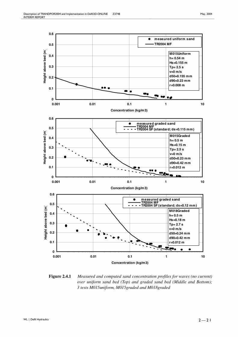
Figure 2.4.1 shows measured sand concentration profiles (based on the pumpedconcentrations) for waves with Hs= 0.15 m and 0.18 m over uniform and graded bedmaterial. The experimental conditions are given in each plot. As can be observed bycomparing the results of Figure 2.4.1Top and Middle (Hs=0.15 m for both cases), the near-bed concentrations are significantly larger (factor 2) for the graded sediment bed (Middle)and the sand concentrations higher up in the water column are somewhat larger for thegraded sediment bed, which is caused by the winnowing of the fine sediments from the bed.Figure 2.4.2 shows measured concentration profiles for combined wave and currentconditions (3 tests). As can be observed, the concentrations are more uniformly distributedover the depth due to the mixing capacity of the current.
2.4.2 Model results
Both the Single-fraction method and the Multi-fraction method have been applied tocompute the sand concentration profiles for the 6 experimental cases. The Multi-fractionmethod has not been used for the uniform sediment case M015U.The results are shown in Figures 2.4.1 and 2.4.2 for 6 cases.The results are:Waves alone (Figure 2.4.1)• the computed sand concentrations based on the SF-method are considerably too small
compared with the measured concentrations in the near-bed region for the uniform sand(Figure 2.4.1Top) due to under-prediction of the reference concentration; the computedconcentrations in the upper layers are slightly too large;
• the computed sand concentrations based on the MF-method show reasonably goodagreement with the measured concentrations in the near-bed region for the graded sand bed(Figure 2.4.1Middle and Bottom), but the computed concentrations higher up in the watercolumn are much too large compared with the measured values; the winnowing effect of thefine fractions is overestimated by the model; the wave-related mixing coefficient is too largefor z>0.1 m.
• the computed reference concentration based on the MF-method is larger than that based onthe SF-method, which is in agreement with the physics involved (larger near-bedconcentrations for graded sediment than for uniform sediment).
Combined current and waves (Figure 2.4.2)• the computed sand concentrations based on the MF-method show reasonably good
agreement with the measured concentrations for the graded sand; the vertical distribution ispredicted rather good, but the reference concentration is somewhat under predicted;
• the computed sand concentrations based on the SF-method are considerably too small if thesuspended sediment size is based on the standard prediction method (ds=0.13 mm≅0.5d50,bed); the computed sand concentrations show reasonably good agreement with themeasured values, if the suspended sediment size is taken (calibrated) as ds= 0.4d50,bed≅0.1mm; the measured suspended sediment sizes vary between ds= 0.35 d50,bed and 0.45 d50,bed.
Description of TRANDPOR2004 and Implementation in Delft3D-ONLINE Z3748 May, 2004 INTERIM REPORT
WL | Delft Hydraulics 2 — 2 1
Figure 2.4.1 Measured and computed sand concentration profiles for waves (no current)over uniform sand bed (Top) and graded sand bed (Middle and Bottom);3 tests M015uniform, M015graded and M018graded
0
0.1
0.2
0.3
0.4
0.5
0.6
0.001 0.01 0.1 1 10
Concentration (kg/m3)
Hei
gh
tab
ove
bed
(m)
measured uniform sand
TR2004 MF
M015Uniformh= 0.54 mHs=0.155 mTp= 2.5 sv=0 m/sd50=0.155 mmd90=0.23 mmr=0.008 m
0
0.1
0.2
0.3
0.4
0.5
0.6
0.001 0.01 0.1 1 10
Concentration (kg/m3)
Hei
gh
tab
ove
bed
(m)
measured graded sandTR2004 MFTR2004 SF (standard; ds=0.115 mm)
M015Gradedh= 0.5 mHs=0.15 mTp= 2.5 sv=0 m/sd50=0.23 mmd90=0.42 mmr=0.012 m
0
0.1
0.2
0.3
0.4
0.5
0.6
0.001 0.01 0.1 1 10
Concentration (kg/m3)
Hei
gh
tab
ove
bed
(m)
measured graded sandTR2004 MFTR2004 SF (standard; ds=0.12 mm)
M018Gradedh= 0.5 mHs=0.18 mTp= 2.7 sv=0 m/sd50=0.24 mmd90=0.42 mmr=0.012 m

Description of TRANDPOR2004 and Implementation in Delft3D-ONLINE Z3748 May, 2004 INTERIM REPORT
WL | Delft Hydraulics 2 — 2 2
Figure 2.4.2 Measured and computed sand concentration profiles for combined currentand waves over graded sand bed; 3 tests M218graded, M220graded andM418graded
0
0.1
0.2
0.3
0.4
0.5
0.6
0.001 0.01 0.1 1 10Concentration (kg/m3)
Hei
gh
tab
ove
bed
(m)
measured graded sandTR2004 SF (ds=0.13 mm; standard)TR2004 MF (10 fractions)TR2004 SF (ds=0.1 mm; calibrated)
M218Gradedh= 0.5 mHs=0.155 mTp= 2.7 sv=0.2 m/sd50=0.26 mmd90=0.42 mm
0 022
0
0.1
0.2
0.3
0.4
0.5
0.6
0.001 0.01 0.1 1 10
Concentration (kg/m3)
Hei
gh
tab
ove
bed
(m)
measured graded sandTR2004 MF (10 fractions)TR2004 SF (ds=0.13 mm; standard)TR2004 SF (ds=0.1 mm; calibrated)
M220Gradedh= 0.52 mHs=0.2 mTp= 2.7 sv=0.17 m/sd50=0.26 mmd90=0.42 mmr=0.022 m
0
0.1
0.2
0.3
0.4
0.5
0.6
0.001 0.01 0.1 1 10
Concentration (kg/m3)
Hei
gh
tab
ove
bed
(m)
measured graded sandTR2004 MF (10 fractions)TR2004 SF (ds=0.135 mm; standard)TR2004 SF (ds=0.1 mm; calibrated)
M418Gradedh= 0.52 mHs=0.15 mTp= 2.6 sv=0.29 m/sd50=0.27 mmd90=0.41 mmr=0.022 m

Description of TRANDPOR2004 and Implementation in Delft3D-ONLINE Z3748 May, 2004 INTERIM REPORT
WL | Delft Hydraulics 3 — 1
3 Sand transport formulations in DELFT3D model
3.1 Introduction
Section 3.2 of this chapter gives a detailed description of the implemented processes inDELFT3D-ONLINE. Sub-sections 3.2.1 and 3.2.2 present overviews of the hydrodynamicsof currents and waves (largely taken from Lesser et al., 2003). Sub-Section 3.2.3 describesthe sediment transport formulations based on TR2004 for non-cohesive sediment followingVan Rijn (1993, 2000 and 2002) which have been implemented in DELFT3D-ONLINE aspart of the present study. Besides the TR2004 approach, DELFT3D-ONLINE offers anumber of extra sediment transport relations for non-cohesive sediment, see Table 3.1below (a detailed overview of Delft3D-Online sand transport approaches is given in Table3.2).
Formula Transport modes Waves IFORM
Engelund-Hansen (1967) Total transport No 1Meyer-Peter-Muller (1948) Bed load transport No 2Swanby (Ackers-White, 1973) Total transport No 3General formula Total transport No 4Bijker (1971) Bed load + suspended Yes 5Van Rijn (1984) Bed load + suspended No 7Soulsby / Van Rijn Bed load + suspended Yes 11Soulsby Bed load + suspended Yes 12Van Rijn (TR2004) Bed load + suspended Yes -1Van Rijn (TR1993) Bed load + suspended Yes 0
Remarks: Application of a total transport formulation implies that total load transport is treated as bed-loadtransport; suspended load transport is assumed to be zero.
Table 3.1 Available sand transport formulations in DELFT3D-ONLINE.
It is emphasized that the implementation as it is reported in this chapter is focussed on theimplementation of the TR2004 formulations regarding suspended sediment size, variableroughness, etc. (see Section 3.2.3). In the present version of Delft3D-ONLINE, theapproximation formulas are for the bed load transport are still used. An extension to includethe complete TR2004 formulations will be done during the course of the project (intra-waveapproach to determine wave-related bed load transport). This upgrade will require a redesignof some parts of the code which is also influenced by upgrades of other parts of the code.The description given here should be seen as a report of the present status of the model. Atthe end of the project a complete overview will be given of the improved Delft3D-ONLINEmodel.

Description of TRANDPOR2004 and Implementation in Delft3D-ONLINE Z3748 May, 2004 INTERIM REPORT
WL | Delft Hydraulics 3 — 2
Type of model Spatialdimension
Transport approach
DELFT-ONLINE
2DH Bed load transporta) Equilibrium transport based on approximation function ofTR2000b) Other equilibrium formulations (See Table 2.1.2)Wave-related suspended transportEquilibrium transport based on approximation method of TR2000Current-related suspended transport1) Depth-averaged sand concentration derived from equilibriumsand transport formulation plus adjustment factor based onmethod of Galappatti2) Equilibrium suspended transport formulations (no adjustment):a)TR2000 (detailed formulations)b)TR2000 (approximation functions)c) Other formulations; see Table 2.1.2Bed roughnessa) specified by userb) roughness predictor
DELFT-ONLINE
3D and2DV
Bed load transporta) Equilibrium transport based on approximation function ofTR2000b) Other equilibrium formulations (See Table 2.1.2)Wave-related suspended transportEquilibrium transport based on approximation method of TR2000Current-related suspended transport1) Concentration derived from advection-diffusion equation2) Reference concentration derived froma) TR2000b) Other formulations (Table 2.1.2); ref concentration iscalculated backwards from equilibrium suspended transport usingcomputed velocity profiles and mixing coefficientBed roughnessa) specified by userb) roughness predictor
Table 3.2 Sand transport approaches in DELFT-MOR and DELFT3D-ONLINE model.
3.2 Model description
3.2.1 Hydrodynamics
The DELFT3D-FLOW module solves the unsteady shallow-water equations in two (depth-averaged) or three dimensions. The system of equations consists of the horizontalmomentum equations, the continuity equation, the transport equation, and a turbulenceclosure model. The vertical momentum equation is reduced to the hydrostatic pressurerelation as vertical accelerations are assumed to be small compared to gravitationalacceleration and are not taken into account. This makes the DELFT3D-FLOW modelsuitable for predicting the flow in shallow seas, coastal areas, estuaries, lagoons, rivers, andlakes. It aims to model flow phenomena of which the horizontal length and time scales aresignificantly larger than the vertical scales.

Description of TRANDPOR2004 and Implementation in Delft3D-ONLINE Z3748 May, 2004 INTERIM REPORT
WL | Delft Hydraulics 3 — 3
The user may choose whether to solve the hydrodynamic equations on a Cartesianrectangular, orthogonal curvilinear (boundary fitted), or spherical grid. In three-dimensionalsimulations a boundary fitted (σ-coordinate) approach is used for the vertical grid direction.For the sake of clarity the equations are presented in their Cartesian rectangular form only.
Vertical σ-coordinate systemThe vertical σ-coordinate is scaled as ( )− ≤ ≤1 0σ
z
d
ζσζ−
=+
(3.2.1)
The flow domain of a 3D shallow water model consists of a number of layers. In a σ-coordinate system, the layer interfaces are chosen following planes of constant σ. Thus, thenumber of layers is constant over the horizontal computational area. For each layer a set ofcoupled conservation equations is solved. The partial derivatives in the original Cartesiancoordinate system are expressed in σ-coordinates by use of the chain rule. This introducesadditional terms (Stelling and Van Kester, 1994).
Generalised Lagrangian mean (GLM) reference frameIn simulations including waves the hydrodynamic equations are written and solved in aGLM reference frame (Andrews and McIntyre, 1978; Groeneweg and Klopman, 1998;and Groeneweg 1999). In GLM formulation the 2DH and 3D flow equations are verysimilar to the standard Eulerian equations, however, the wave-induced driving forcesaveraged over the wave period are more accurately expressed. The relationship between theGLM velocity and the Eulerian velocity is given by:
s
s
U u u
V v v
= += +
(3.2.2)
where U and V are GLM velocity components, u and v are Eulerian velocity components,
and su and sv are the Stokes’ drift components. For details and verification results we refer
to Walstra et al. (2000).
Hydrostatic pressure assumptionUnder the so-called “shallow water assumption” the vertical momentum equation reduces tothe hydrostatic pressure equation. Under this assumption vertical acceleration due tobuoyancy effects or sudden variations in the bottom topography is not taken into account.The resulting expression is:
Pg h
∂ ρ∂σ
= − (3.2.3)
Horizontal momentum equationsThe horizontal momentum equations are

Description of TRANDPOR2004 and Implementation in Delft3D-ONLINE Z3748 May, 2004 INTERIM REPORT
WL | Delft Hydraulics 3 — 4
20
20
1 1
1 1
x x x V
y y y V
U U U U uU v fV P F M
t x y h h
V V V V vU V fU P F M
t x y h h
∂ ∂ ∂ ω ∂ ∂ ∂ν∂ ∂ ∂ ∂σ ρ ∂σ ∂σ
∂ ∂ ∂ ω ∂ ∂ ∂ν∂ ∂ ∂ ∂σ ρ ∂σ ∂σ
+ + + − = − + + +
+ + + − = − + + +
(3.2.4)
in which the horizontal pressure terms, Px and Py , are given by (Boussinesq
approximations)
0
0 0
0
0 0
1
1
x
y
hP g g d
x x x
hP g g d
y y y
σ
σ
∂ζ ∂ρ ∂σ ∂ρ σρ ∂ ρ ∂ ∂ ∂σ
∂ζ ∂ρ ∂σ ∂ρ σρ ∂ ρ ∂ ∂ ∂σ
′ ′= + + ′
′ ′= + + ′
∫
∫
(3.2.5)
The horizontal Reynold’s stresses, Fx and Fy , are determined using the eddy viscosity
concept (e.g. Rodi, 1984). For large scale simulations (when shear stresses along closedboundaries may be neglected) the forces Fx and Fy reduce to the simplified formulations
2 2 2 2
2 2 2 2x H y H
U U V VF F
x y x y
∂ ∂ ∂ ∂ν ν∂ ∂ ∂ ∂
= + = +
(3.2.6)
in which the gradients are taken along σ-planes. In Eq. (3.2.4) Mx and My represent thecontributions due to external sources or sinks of momentum (external forces by hydraulicstructures, discharge or withdrawal of water, wave stresses, etc.).
Continuity equationThe depth-averaged continuity equation is given by
hU hVS
t x y
∂ ∂∂ζ∂ ∂ ∂
+ + = (3.2.7)
in which S represents the contributions per unit area due to the discharge or withdrawal ofwater, evaporation, and precipitation.
Transport equationThe advection-diffusion equation reads
[ ] [ ] [ ] ( )
1H H V
hc hUc hVc c
t x y
c c ch D D D hS
x x y y h
∂ ∂ ∂ ∂ ω∂ ∂ ∂ ∂σ
∂ ∂ ∂ ∂ ∂ ∂∂ ∂ ∂ ∂ ∂σ ∂σ
+ + + =
+ + +
(3.2.8)

Description of TRANDPOR2004 and Implementation in Delft3D-ONLINE Z3748 May, 2004 INTERIM REPORT
WL | Delft Hydraulics 3 — 5
in which S represents source and sink terms per unit area.
In order to solve these equations the horizontal and vertical viscosity (ν H and νV ) and
diffusivity ( DH and DV ) need to be prescribed. In DELFT3D-FLOW the horizontal
viscosity and diffusivity are assumed to be a superposition of three parts: 1) molecularviscosity, 2) “3D turbulence”, and 3) “2D turbulence”. The molecular viscosity of the fluid(water) is a constant value O(10-6). In a 3D simulation “3D turbulence” is computed by theselected turbulence closure model (see the turbulence closure model section below). “2Dturbulence” is a measure of the horizontal mixing that is not resolved by advection on thehorizontal computational grid. 2D turbulence values may either be specified by the user as aconstant or space-varying parameter, or can be computed using a sub-grid model forhorizontal large eddy simulation (HLES). The HLES model available in DELFT3D-FLOWis based on theoretical considerations presented by Uittenbogaard (1998) and is fullydiscussed by Van Vossen (2000).
For use in the transport equation, the vertical eddy diffusivity is scaled from the verticaleddy viscosity according to
DVV
c
=νσ
(3.2.9)
in which σ c is the Prandtl-Schmidt number given by
σ σ σc c F Ri= 0 b g (3.2.10)
where σ c0 is purely a function of the substance being transported. In the case of the
algebraic turbulence model, F Riσ b g is a damping function that depends on the amount of
density stratification present via the gradient Richardson’s number (Simonin et al., 1989).
The damping function, F Riσ b g , is set equal to 1.0 if the k − ε turbulence model is used, as
the buoyancy term in the k − ε model automatically accounts for turbulence-dampingeffects caused by vertical density gradients.
We note that the vertical eddy diffusivity used for calculating the transport of “sand”sediment constituents may, under some circumstances, vary somewhat from that given byEq. (3.2.9) above. The diffusion coefficient used for sand sediment is described in moredetail in Section 3.2.3.
Turbulence closure modelsSeveral turbulence closure models are implemented in DELFT3D-FLOW. All models arebased on the so-called “eddy viscosity” concept (Kolmogorov, 1942; Prandtl, 1945). Theeddy viscosity in the models has the following form
ν µV c L k= ′ (3.2.11)

Description of TRANDPOR2004 and Implementation in Delft3D-ONLINE Z3748 May, 2004 INTERIM REPORT
WL | Delft Hydraulics 3 — 6
in which ′cµ is a constant determined by calibration, L is the mixing length, and k is the
turbulent kinetic energy.
Two types of turbulence closure models are available in DELFT3D-FLOW. The first is the“algebraic” turbulence closure model that uses algebraic/analytical formulas to determine kand L and therefore the vertical eddy viscosity. The second is the k − ε turbulence closuremodel in which both the turbulent energy k and the dissipation ε are produced byproduction terms representing shear stresses at the bed, surface, and in the flow. The“concentrations” of k and ε in every grid cell are then calculated by transport equations.The mixing length L is determined from ε and k according to
L ck k
D=ε
(3.2.12)
in which cD is another calibration constant.
3.2.1.1 Boundary Conditions
In order to solve the systems of equations, the following boundary conditions are required:
Bed and free surface boundary conditionsIn the σ-coordinate system the bed and the free surface correspond with σ-planes. Thereforethe vertical velocities at these boundaries are simply
ω ω− = =1 0 0 0b g b gand (3.2.13)
Friction is applied at the bed as follows:
1 1
byV bx Vu v
h hσ σ
τν ∂ τ ν ∂∂σ ρ ∂σ ρ=− =−
= = (3.2.14)
where bxτ and byτ are bed shear stress components that include the effects of wave-current
interaction.
Friction due to wind stress at the water surface may be included in a similar manner. For thetransport boundary conditions the vertical diffusive fluxes through the free surface and bedare set to zero.
Lateral boundary conditionsAlong closed boundaries the velocity component perpendicular to the closed boundary is setto zero (a free-slip condition). At open boundaries one of the following types of boundaryconditions must be specified: water level, velocity (in the direction normal to the boundary),discharge, or Riemann (weakly reflective boundary condition, Verboom and Slob, 1984).Additionally, in the case of 3D models, the user must prescribe the use of either a uniform orlogarithmic velocity profile at inflow boundaries.

Description of TRANDPOR2004 and Implementation in Delft3D-ONLINE Z3748 May, 2004 INTERIM REPORT
WL | Delft Hydraulics 3 — 7
For the transport boundary conditions we assume that the horizontal transport of dissolvedsubstances is dominated by advection. This means that at an open inflow boundary aboundary condition is needed. During outflow the concentration must be free. DELFT3D-FLOW allows the user to prescribe the concentration at every σ−layer using a time series.For sand sediment fractions the local equilibrium sediment concentration profile may beused.
3.2.1.2 Solution Procedure
DELFT3D-FLOW is a numerical model based on finite differences. To discretise the 3Dshallow water equations in space, the model area is covered by a rectangular, curvilinear, orspherical grid. It is assumed that the grid is orthogonal and well-structured. The variablesare arranged in a pattern called the Arakawa C-grid (a staggered grid). In this arrangementthe water level points (pressure points) are defined in the centre of a (continuity) cell; thevelocity components are perpendicular to the grid cell faces where they are situated.
HydrodynamicsAn alternating direction implicit (ADI) method is used to solve the continuity and horizontalmomentum equations (Leendertse 1987). The advantage of the ADI method is that theimplicitly integrated water levels and velocities are coupled along grid lines, leading tosystems of equations with a small bandwidth. Stelling (1983) extended the ADI method ofLeendertse with a special approach for the horizontal advection terms. This approach splitsthe third-order upwind finite-difference scheme for the first derivative into two second-orderconsistent discretisations, a central discretisation and an upwind discretisation, which aresuccessively used in both stages of the ADI-scheme. The scheme is denoted as a “cyclicmethod” (Stelling and Leendertse, 1991). This leads to a method that is computationallyefficient, at least second-order accurate, and stable at Courant numbers of up toapproximately 10. The diffusion tensor is redefined in the σ-coordinate system assumingthat the horizontal length scale is much larger than the water depth (Mellor and Blumberg,1985) and that the flow is of boundary-layer type.
The vertical velocity, ω, in the σ-coordinate system is computed from the continuityequation,
[ ] [ ]hU hV
t x y
∂ ∂∂ω ∂ζ∂σ ∂ ∂ ∂
= − − − (3.2.15)
by integrating in the vertical from the bed to a level σ. At the surface the effects ofprecipitation and evaporation are taken into account. The vertical velocity, ω, is defined atthe iso-σ-surfaces. ω is the vertical velocity relative to the moving σ-plane and may beinterpreted as the velocity associated with up- or down-welling motions. The verticalvelocities in the Cartesian coordinate system can be expressed in the horizontal velocities,water depths, water levels, and vertical coordinate velocities according to:
h h hw U V
x x y y t t
∂ ∂ζ ∂ ∂ζ ∂ ∂ζω σ σ σ∂ ∂ ∂ ∂ ∂ ∂
= + + + + + + (3.2.16)

Description of TRANDPOR2004 and Implementation in Delft3D-ONLINE Z3748 May, 2004 INTERIM REPORT
WL | Delft Hydraulics 3 — 8
TransportThe transport equation is formulated in a conservative form (finite-volume approximation)and is also solved using the so-called “cyclic method” (Stelling and Leendertse, 1991). Forsteep bottom slopes in combination with vertical stratification, horizontal diffusion along σ-planes introduces artificial vertical diffusion (Huang and Spaulding, 1996). DELFT3D-FLOW includes an algorithm to approximate the horizontal diffusion along z-planes in a σ-coordinate framework (Stelling and Van Kester, 1994). In addition, a horizontal Foresterfilter (Forester, 1979) based on diffusion along σ-planes is applied to remove any negativeconcentration values that may occur. The Forester filter is mass conserving and does notinflict significant amplitude losses in sharply peaked solutions.
3.2.2 Waves
3.2.2.1 General
Wave effects can also be included in a DELFT3D-FLOW simulation by running the separateDELFT3D-WAVE module. A call to the DELFT3D-WAVE module must be made prior torunning the FLOW module. This will result in a communication file being stored whichcontains the results of the wave simulation (RMS wave height, peak spectral period, wavedirection, mass fluxes, etc) on the same computational grid as is used by the FLOW module.The FLOW module can then read the wave results and include them in flow calculations.Wave simulations may be performed using the 2nd generation wave model HISWA(Holthuijsen et al., 1989) or the 3rd generation SWAN model (Holthuijsen et al., 1993). Asignificant practical advantage of using the SWAN model is that it can run on the samecurvilinear grids as are commonly used for DELFT3D-FLOW calculations; thissignificantly reduces the effort required to prepare combined WAVE and FLOWsimulations.
In situations where the water level, bathymetry, or flow velocity field change significantlyduring a FLOW simulation, it is often desirable to call the WAVE module more than once.The computed wave field can thereby be updated accounting for the changing water depthsand flow velocities. This functionality is possible by way of the MORSYS steering modulethat can make alternating calls to the WAVE and FLOW modules. At each call to the WAVEmodule the latest bed elevations, water elevations and, if desired, current velocities aretransferred from FLOW.
3.2.2.2 Wave Effects
In coastal seas wave action may influence morphology for a number of reasons. Thefollowing processes are presently accounted for in DELFT3D-FLOW.
1. Wave forcing due to breaking (by radiation stress gradients) is modelled as a shearstress at the water surface (Svendsen, 1985; Stive and Wind, 1986). This radiationstress gradient is modelled using the simplified expression of Dingemans et al.(1987), where contributions other than those related to the dissipation of waveenergy are neglected. This expression is as follows,

Description of TRANDPOR2004 and Implementation in Delft3D-ONLINE Z3748 May, 2004 INTERIM REPORT
WL | Delft Hydraulics 3 — 9
DM k
ω=""
(3.2.17)
in which M"
= Forcing due to radiation stress gradients (N/m2), D = Dissipation due
to wave breaking (W/m2), ω = Angular wave frequency (rad/s), and k"
= Wavenumber vector (rad/m).
2. The effect of the enhanced bed shear stress on the flow simulation is accounted forby following the parameterisations of Soulsby et al. (1993). Of the several modelsavailable, the simulations presented in this report use the wave-current interactionmodel of Fredsøe (1984).
3. The wave-induced mass flux is included and is adjusted for the vertically non-uniform Stokes drift (Walstra et al., 2000).
4. The additional turbulence production due to dissipation in the bottom wave boundarylayer and due to wave white capping and breaking at the surface is included as extraproduction terms in the k − ε turbulence closure model (Walstra et al., 2000).
5. Streaming (a wave-induced current in the bottom boundary layer directed in thedirection of wave propagation) is modelled as an additional shear stress acting acrossthe thickness of the bottom wave boundary layer (Walstra et al., 2000).
Processes 3, 4, and 5 have only recently been included in DELFT3D-FLOW and areessential if the (wave-averaged) effect of waves on the flow is to be correctly represented in3D simulations. This is especially important for the accurate modelling of sedimenttransport in a near-shore coastal zone.
3.2.3 Sediment dynamics and bed level evolution
For the transport of non-cohesive sediment, Van Rijn's (1993, 2000, or 2004) approach isfollowed by default. The user can also specify a number of other transport formulations (seeTable 2.1.1) The transport relations are a mix of Van Rijn’s TRANSPOR2000 (TR2000) andapproximation formulations (Van Rijn, 2002; Van Rijn and Walstra, 2003). In all theseformulations Van Rijn distinguishes between bed load and suspended load which both havea wave-related and current-related contribution:
, ,
, ,
s s c s w
b b c b w
S S S
S S S
= +
= +(3.2.18)
in which Ss is the suspended transport, Sb the bed load transport, Ss,c and Ss,w the respectivecurrent-related and wave-related suspended transports, Sb,c and Sb,w the respective current-related and wave-related bed load transports. The transport gradients in x- and y-directionare being used in the sediment continuity equation to determine the bed level changes, asfollows:
( ) ( ), ,, , 0b y s yb x s xb
S SS Sz
t x y
∂ +∂ +∂+ + =
∂ ∂ ∂(3.2.19)
with:

Description of TRANDPOR2004 and Implementation in Delft3D-ONLINE Z3748 May, 2004 INTERIM REPORT
WL | Delft Hydraulics 3 — 1 0
Sb,x= Sb,c,x+Sb,w,x being the bed-load transport in x-direction (u-velocity direction),Sb,y= Sb,c,y+Sb,w,y being the bed-load transport in y-direction (v-velocity direction),Ss,x= Ss,c,x+Ss,w,x being the suspended load transport in x-direction (u-velocity direction),Ss,y= Ss,c,y+Ss,w,y being the suspended load transport in y-direction (v-velocity direction),and Sb,c and Sb,w are the current-related and wave-related bed load transports, Ss,c and Ss,w arethe current-related and wave-related suspended load transports (in x and y directions).
The bed-load transport contributions are based on a quasi-steady approach, which impliesthat the bed-load transport is assumed to respond almost instantaneously to orbital velocitieswithin the wave cycle and to the prevailing current-velocity. Similarly, the wave-relatedsuspended load transport contribution is assumed to respond almost instantaneously to theorbital velocities. These transport contributions (Sb,c, Sb,w and Ss,w) can be formulated interms of time-averaged (over the wave period) parameters resulting in relatively simpletransport expressions.
The current-related suspended load transport is based on the variation of the suspended sandconcentration field due to the effects of currents and waves. Using a 2DH-approach, thesand concentration field is described in terms of the depth-averaged equilibrium sandconcentration derived from equilibrium transport formulations and an adjustment factorbased on the (numerical) method of Galappatti. Using a 3D-approach, the sandconcentration field is based on the numerical solution of the 3D advection-diffusionequation (see Sub-Section 3.2.3.1).
The upgrade of TRANSPOR2000 to TRANSPOR2004 concerns the following points:1. Predictor of bed roughness, see Eqs. (3.2.35), (3.2.36), (3.2.37) and (3.2.40);2. Predictor of suspended sediment size, see Eq. (3.2.23);3. Grain roughness and friction factor, see Eq. (3.2.46);4. Wave-induced orbital velocities near the bed, see Eq. (3.2.56);5. Wave-induced bed-shear stress, see Eq. (3.2.50);6. Shields criterion for fine sand, see Eq. (3.2.53);7. wave-related suspended transports, see Eq. (3.2.67);8. Mixing near the bed, see Eq. (3.2.26);9. Reference concentration, see Eqs. (3.2.33);
10. Modification of the thickness of the effective near-bed sediment mixing layer sδ , see
Eq. (3.2.27);
11. Modification of the thickness of the wave boundary layer wδ , see Eq. (3.2.28);
12. The expressions for the parametric mixing coefficients have also been modified (εs,w,max,εs,w,bed), see Eq. (3.2.26);
13. The wave related efficiency factor (µw), see Eq. (3.2.49).
3.2.3.1 3-Dimensional advection-diffusion equation for current-related suspended transport
Three-dimensional transport of suspended sediment is calculated by solving the three-dimensional advection-diffusion (mass-balance) equation for the suspended sediment:

Description of TRANDPOR2004 and Implementation in Delft3D-ONLINE Z3748 May, 2004 INTERIM REPORT
WL | Delft Hydraulics 3 — 1 1
( )( ) ( )( ) ( ) ( )
( ) ( ) ( )( ) ( ) ( ), , , 0,
s
s x s y s z
w w cc uc vc
t x y z
c c c
x x y y z zε ε ε
∂ −∂ ∂ ∂+ + + +
∂ ∂ ∂ ∂
∂ ∂ ∂ ∂ ∂ ∂− − − = ∂ ∂ ∂ ∂ ∂ ∂
! !! ! !
! ! !! ! !
(3.2.20)
where:( )c ! mass concentration of sediment fraction ( )! [kg/m3],
,u v and w flow velocity components [m/s],( ) ( ) ( ), , , ,and,s x s y s y s zε ε ε! ! ! eddy diffusivities of sediment fraction ( )! [m2/s],
( )sw ! sediment settling velocity of sediment fraction ( )! ;
hindered settling effects are taken into account [m/s].
The local flow velocities and eddy diffusivities are based on the results of the hydrodynamiccomputations. Computationally, the three-dimensional transport of sediment is computed inexactly the same way as the transport of any other conservative constituent, such as salinity,heat, and constituents. There are, however, a number of important differences betweensediment and other constituents. For example, the exchange of sediment between the bedand the flow, and the settling velocity of sediment under the action of gravity. Theseadditional processes for sediment are obviously of critical importance. Other processes suchas the effect that sediment has on the local mixture density, and hence on turbulencedamping, can also be taken into account. In addition, if a net flux of sediment from the bedto the flow, or vice versa, occurs then the resulting change in the bathymetry shouldinfluence subsequent hydrodynamic calculations. The formulation of several of theseprocesses are sediment-type specific, this especially applies for sand and mud.
Based on the computed sand concentration field, the current-related suspended transportrates in x- and y-directions are computed as:
, , ,
, , ,
h
s c x s x
a
h
s c y s y
a
cS uc dz
x
cS vc dz
y
ε
ε
∂ = − ∂
∂= − ∂
∫
∫(3.2.21)
3.2.3.2 Suspended sediment size and sediment settling velocity
The settling velocity of a non-cohesive (“sand”) sediment fraction is computed followingthe method of Van Rijn (1993). The formulation used depends on the diameter of thesediment in suspension:

Description of TRANDPOR2004 and Implementation in Delft3D-ONLINE Z3748 May, 2004 INTERIM REPORT
WL | Delft Hydraulics 3 — 1 2
( ) 2
,0
0.5( ) 3
,0 2
0.5( ),0
( 1), 65 100
18
0.01( 1)101 1 , 100 1000
1.1 ( 1) , 1000
ss s
ss s
s s s
s g dw m d m
s g dw m d m
d
w s g d m d
µ µυ
ν µ µυ
µ
−= < ≤
− = + − < ≤
= − <
( )( )
( )( )
( ) ( )
! !!
! !!
! ! !
(3.2.22)
where:
( )s ! relative density of sediment fraction ( )! .
( )d ! representative diameter of sediment fraction ( )! .
υ kinematic viscosity coefficient of water [m2/s].
If only one sediment fraction is used, the representative diameter of the suspended sedimentcan be determined based on two options via the user-defined properties SEDDIA (d50 of bed
material) and IOPSUS (options for determining sd is determined based on the mobility
parameter, M, see Eq. (3.2.60), as follows:
1) a suspended sediment diameter based in the following expression:
( )5050, 50
10
50
min 0.5 1 0.0006 1 550 250
250
s
s
dd d d for
d
d d for
ψ ψ
ψ
= + − − < = ≥
(3.2.23)
for ψ see Eq. (3.2.38),2) ds=FACDSS d50; based on a multiplication of the user-defined properties SEDDIA (d50
of bed material) and FACDSS (see also remark)
Remark:In the case of non-uniform bed material Van Rijn (1993) concluded that, on the basis ofmeasurements, ds is in the range of 60% to 100% of d50 of the bed material. If the bedmaterial is very widely graded (well sorted) consideration should be given to using severalsediment fractions to model its behaviour more accurately.
3.2.3.3 Sediment mixing and dispersion
DELFT3D-FLOW supports four turbulence closure models:• Constant coefficient.• Algebraic eddy viscosity closure model.• k L− turbulence closure model.
• k ε− turbulence closure model.
The first is a simple constant value which is specified by the user. A constant eddy viscositywill lead to parabolic vertical velocity profiles (laminar flow). The other three turbulenceclosure models are based on the eddy viscosity concept of Kolmogorov (1942) and Prandtl
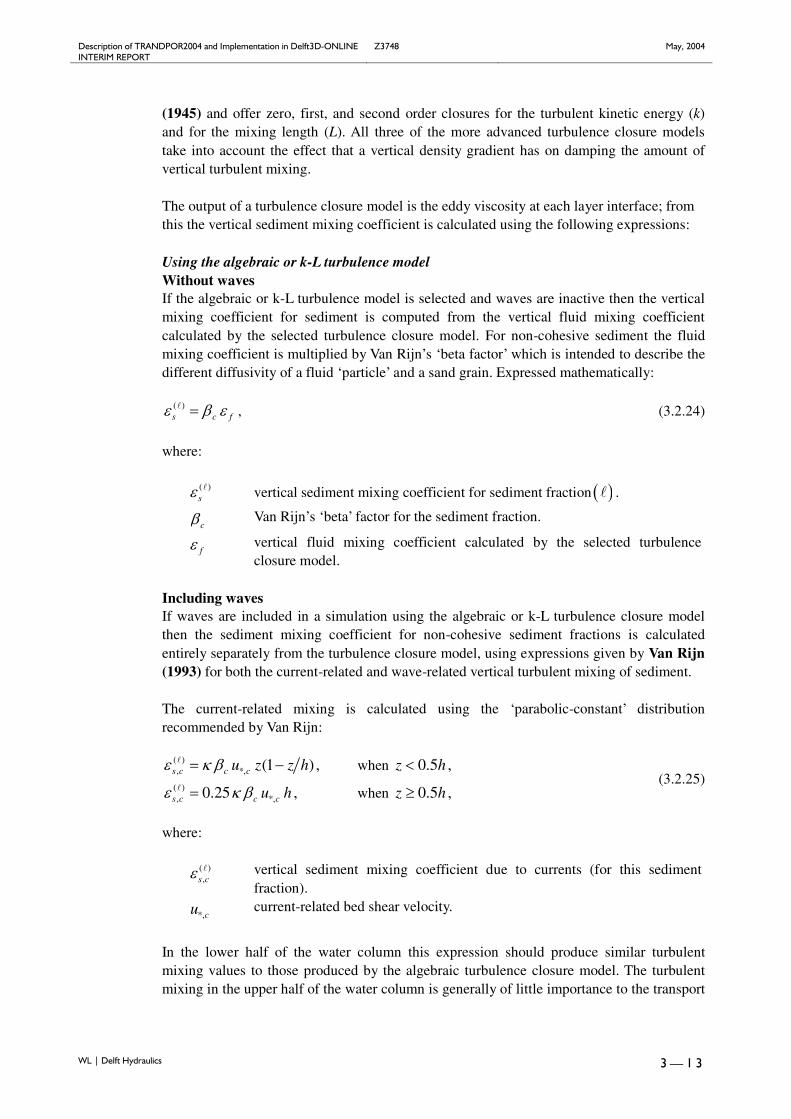
Description of TRANDPOR2004 and Implementation in Delft3D-ONLINE Z3748 May, 2004 INTERIM REPORT
WL | Delft Hydraulics 3 — 1 3
(1945) and offer zero, first, and second order closures for the turbulent kinetic energy (k)and for the mixing length (L). All three of the more advanced turbulence closure modelstake into account the effect that a vertical density gradient has on damping the amount ofvertical turbulent mixing.
The output of a turbulence closure model is the eddy viscosity at each layer interface; fromthis the vertical sediment mixing coefficient is calculated using the following expressions:
Using the algebraic or k-L turbulence modelWithout wavesIf the algebraic or k-L turbulence model is selected and waves are inactive then the verticalmixing coefficient for sediment is computed from the vertical fluid mixing coefficientcalculated by the selected turbulence closure model. For non-cohesive sediment the fluidmixing coefficient is multiplied by Van Rijn’s ‘beta factor’ which is intended to describe thedifferent diffusivity of a fluid ‘particle’ and a sand grain. Expressed mathematically:
( )s c fε β ε=! , (3.2.24)
where:
( )sε! vertical sediment mixing coefficient for sediment fraction ( )! .
cβ Van Rijn’s ‘beta’ factor for the sediment fraction.
fε vertical fluid mixing coefficient calculated by the selected turbulenceclosure model.
Including wavesIf waves are included in a simulation using the algebraic or k-L turbulence closure modelthen the sediment mixing coefficient for non-cohesive sediment fractions is calculatedentirely separately from the turbulence closure model, using expressions given by Van Rijn(1993) for both the current-related and wave-related vertical turbulent mixing of sediment.
The current-related mixing is calculated using the ‘parabolic-constant’ distributionrecommended by Van Rijn:
( ), *,
( ), *,
when
when
(1 ) , 0.5 ,
0.25 , 0.5 ,
s c c c
s c c c
u z z h z h
u h z h
ε κ β
ε κ β
= − <
= ≥
!
!(3.2.25)
where:
( ),s cε ! vertical sediment mixing coefficient due to currents (for this sediment
fraction).
*,cu current-related bed shear velocity.
In the lower half of the water column this expression should produce similar turbulentmixing values to those produced by the algebraic turbulence closure model. The turbulentmixing in the upper half of the water column is generally of little importance to the transport

Description of TRANDPOR2004 and Implementation in Delft3D-ONLINE Z3748 May, 2004 INTERIM REPORT
WL | Delft Hydraulics 3 — 1 4
of ‘sand’ sediment fractions as sediment concentrations in the upper half of the watercolumn are low.
The wave- related mixing is calculated following Van Rijn (1993, 2000). In this case VanRijn recommends a step type distribution over the vertical, with a linear transition betweenthe two steps, see Figure 2.1.1.
Figure 3.2.1 Sediment mixing coefficient (Van Rijn 1993).
The expressions used to set this distribution are, using updated TR2004 relation:
( )
( ) ( ) ( ) ( ), , , ,
( ) ( ), ,max
( )( ) ( ) ( ) ( ) ( ), , ,max , ( )
when
when
when
0.018 , ,
0.035, 0.5 ,
, 0.5 ,0.5
s w s bed w s w r s
br ss w s
p
ss w s bed s s bed s
s
U z
hHz h
T
zz h
h
δε ε β δ δ
γε ε
δε ε ε ε δδ
= = ≤
= = ≥
−= + − < < −
! ! ! !
! !
!! ! ! ! !
!
(3.2.26)
where ( )sδ! (the thickness of the near-bed sediment mixing layer) is estimated by using the
updated TR2004 relation:
{ }( ) max 0.05,min 0.2,2s br wδ γ δ= ! (3.2.27)
where:
wδ thickness of the wave boundary layer (updated TR2004 relation):0.25
, ,
0.36ws w r
AA
kδ
δδ−
=
(3.2.28)
brγ empirical coefficient related to wave breaking:

Description of TRANDPOR2004 and Implementation in Delft3D-ONLINE Z3748 May, 2004 INTERIM REPORT
WL | Delft Hydraulics 3 — 1 5
0.5
1 0.4 1 0.4s sbr br
H Hand for
h hγ γ = + − = ≤
(3.2.29)
, ,s w rk wave-related bed roughness (as calculated for suspended sediment transport,see Eq. (3.2.40)).
The total vertical sediment mixing coefficient according to Van Rijn is based on the sum ofthe squares:
( ) ( )2 ( )2, ,s s c s wε ε ε= +! ! ! , (3.2.30)
where sε is the vertical sediment diffusion coefficient used in the suspended sediment
transport calculations for this sediment fraction.
Using the k ε− turbulence modelIn the case of the k ε− turbulence closure model the vertical sediment mixing coefficientcan be calculated directly from the vertical fluid mixing coefficient calculated by theturbulence closure model, using the following expression:
( ) ( )s cw fε β ε=! ! , (3.2.31)
where:( )sε! vertical sediment mixing coefficient of sediment fraction ( )! .
( )cwβ ! the effective Van Rijn’s ‘beta’ factor of sediment fraction ( )! . It consists of a
wave and current related contribution:2
( )( )
,
1 2 .scw
cw
w
uβ
∗
= +
!! (3.2.32)
*,cwu combined wave and current-related shear velocity
fε vertical fluid mixing coefficient calculated by the k ε− turbulence closuremodel
This implies that the value of ( )cwβ ! is space (and time) varying, however it is constant over
the depth of the flow. In addition, due to the limited knowledge of the physical processes
involved, the beta-factor ( )cwβ ! is limited to the range ( )1 1.5cwβ< <! .
Remark:• The k ε− turbulence closure model has been extended by Walstra et al. (2000) to
include the three-dimensional effects of waves on the mixing (via the frictional bottomdissipation and wave breaking dissipation).

Description of TRANDPOR2004 and Implementation in Delft3D-ONLINE Z3748 May, 2004 INTERIM REPORT
WL | Delft Hydraulics 3 — 1 6
3.2.3.4 Reference concentration
For non-cohesive sediment (e.g. sand), we follow the method of Van Rijn (1993) for thecombined effect of waves and currents. The reference height is updated for TR2004 andnow reads:
{ }, , , ,max 0.5 ,0.5 ,0.01s c r s w ra k k= , (3.2.33)
where:
a Van Rijn’s reference height.
, ,s c rk current-related bed roughness height due to small-scale ripples (seeoptions below).
, ,s w rk wave-related bed roughness height due to small-scale ripples (seeoptions below).
With the keyword IOPKCW the user has three options to calculate , ,s c rk (and , ,s w rk ):
1) , ,s c rk derived from current-related effective roughness height as determined in the
FLOW module (spatially varying) and , ,s w rk specified by user (constant in space).
2) , ,s c rk and , ,s w rk specified by the user (constant in space).
3) , ,s c rk and , ,s w rk determined by the roughness predictor as derived in this report.
The total physical current-related roughness kc is calculated as:
( )0.52 2 2, , , , , , ,s c s c r s c mr s c dk k k k= + + (3.2.34)
which is based on a summation of the current-related roughness due to ripples ( , ,s c rk ),
mega-ripples ( , ,s c mrk ) and dunes ( , ,s c dk , rivers only).
The current-related roughness due to ripples is estimated as:
( ), , 50
, , 50
, , 50
150 0 50 ( , )
182.5 0.65 50 250 ( , )
20 250 ( )
s c r
s c r
s c r
k d and lower wave current regime SWR ripples
k d and upper wave current regime sheet flow
k d and linear approach in transitional regime
ψ
ψ ψ
ψ
= ≤ ≤ −
= − < < −
= ≥
(3.2.35)
The current-related roughness due to mega-ripples reads:
( ), ,
, ,
, ,
, , ,
0.01 0 50 1 0.3
0.011 0.00002 50 550 1 0.3
0 550 1 0.3
0.2
s c mr R
s c mr R
s c mr R
s c mr MAX
k h and and h and v
k h and and h and v
k and and h and v
k
ψ
ψ ψ
ψ
= ≤ ≤ > >
= − < < > >
= ≥ > >
=
(3.2.36)

Description of TRANDPOR2004 and Implementation in Delft3D-ONLINE Z3748 May, 2004 INTERIM REPORT
WL | Delft Hydraulics 3 — 1 7
The current-related roughness due to dunes in rivers reads:
( ), ,
, ,
, ,
, , ,
0.0004 0 100 1 0.3
0.048 0.0008 100 600 1 0.3
0 600 1 0.3
1.0
s c d R
s c d R
s c d R
s c d MAX
k h and and h and v
k h and and h and v
k and and h and v
k
ψ ψ
ψ ψ
ψ
= ≤ ≤ > >
= − < < > >
= ≥ > >
=
(3.2.37)
in which ψ is the mobility parameter:
( )2
501wcu
s gdψ =
−, (3.2.38)
where:
2 2 2 coswc R Ru U v U vδ δ ϕ= + + , (3.2.39)
in which Uδ is the peak orbital velocity near bed based on linear wave theory, Rv is the
magnitude of an equivalent depth-averaged velocity computed from the velocity in thebottom computational layer, assuming a logarithmic velocity profile, ϕ is the angle betweenwave and current motion, Hs the significant wave height, k is the wave number (=2π/L,where L is the wave length derived from (L/Tp±vR)2=gL tanh(2πh/L)/(2π)).
In line with this, it is proposed that the physical wave-related roughness of small-scaleripples is given by:
( )
, , 50
, , 50
, , 50
150 50(lower wave-current regime, SWR ripples)
20 250(upper wave-current regime, sheet flow)
182.5 0.65 50 250(linear approach in transitional regime)
s w r
s w r
s w r
k d for
k d for
k d for
ψ
ψ
ψ ψ
= ≤
= ≥
= − < <
(3.2.40)
This predictor is assumed to be valid for relatively fine sand with d50 in the range of 0.1 to0.5 mm. An estimate of the bed roughness for coarse particles (d50>0.5 mm) can be obtainedby using Eq. (3.2.40) for d50=0.5 mm. Thus, d50=0.5 mm for d50≥0.5 mm resulting in amaximum bed roughness height of 0.075 m (upper limit). The lower limit will beks,w,r=15d50= 0.0015 m for sand with d50≤0.1 mm.Larger scale wave-induced ripples (often known as ‘long wave ripples’ may be present, butthe physical roughness of these types of ripples is assumed to be zero, as flow separation isnot likely to occur.
Calculation of the reference concentrationThe reference concentration is calculated in accordance with Van Rijn (2000), but anadditional factor η is introduced (and monitored) to reflect the presence of multiple
sediment fractions. The resulting expression is:

Description of TRANDPOR2004 and Implementation in Delft3D-ONLINE Z3748 May, 2004 INTERIM REPORT
WL | Delft Hydraulics 3 — 1 8
( )( )
1.5( ) ( )50( ) ( ) ( )
s 0.3( )0.015
a
a
d Tc SUS
a Dη ρ
∗
=! !
! ! !
!(3.2.41)
where:
( )ac ! mass concentration at reference height a.
SUS multiplication factor specified in the morphological input file.
In order to evaluate this expression the following quantities must be calculated:
( )η ! relative availability of sediment fraction:
( ) mass of fraction ( ) in mixing layer
total mass of sediment in mixing layerη =!
!. (3.2.42)
( )D∗! non-dimensional particle diameter:
1( ) 3
( ) ( )50 2
( 1)s gD d
υ∗
−=
!! ! . (3.2.43)
( )aT ! non-dimensional bed-shear stress:
( ) ( ) ( )( ) , ,
( )
( )c b cw w b w cra
cr
Tµ τ µ τ τ
τ+ −
=! ! !
!! . (3.2.44)
( )cµ! efficiency factor current:
( )( ) cc
c
f
fµ
′=
!! . (3.2.45)
( )cf ′! gain related friction factor:
2
( )10 ( )
90
120.24 logc
hf
d
−
′ =
!! . (3.2.46)
( )cf! total current-related friction factor:
2
( )10
,
120.24 logc
s c
hf
k
−
=
! . (3.2.47)
,b cwτ bed shear stress due to current in the presence of waves.
Note that the bed shear velocity *u is calculated in such a way that Van
Rijn’s wave-current interaction factor cwα is not required.2
, *b cw w uτ ρ= , (3.2.48)
( )wµ! efficiency factor waves was recalibrated for the TR2004 formula:
( )
*
( ), *
( ), *
0.7
0.35 2
0.14 5
w
w MAX
w MIN
D
for D
for D
µ
µ
µ
=
= <
= >
!
!
!
, (3.2.49)

Description of TRANDPOR2004 and Implementation in Delft3D-ONLINE Z3748 May, 2004 INTERIM REPORT
WL | Delft Hydraulics 3 — 1 9
,b wτ bed shear stress due to waves (updated in TR2004):
( )2
, ,
1
4b w w w rf Uδτ ρ= (3.2.50)
wf total wave-related friction factor:0.19
, ,
exp 6 5.2ws w r
Af
kδ
− = − +
. (3.2.51)
( )crτ ! critical bed shear stress:
( ) ( )3( ) ( ) ( ) ( )501cr mud s w crp gdτ ρ ρ θ= + −! ! ! ! . (3.2.52)
( )crθ ! threshold parameter ( )
crθ ! is calculated according to the classical Shields
curve as modelled by Van Rijn (1993) as a function of the non-dimensional grain size D*. This avoids the need for iteration. Note that,
for clarity, in this expression the symbol D∗ has been used where ( )D∗!
would be more correct:( ) 0.5
* *
( ) 0.64* *
( ) 0.1* *
( ) 0.29* *
( )*
0.115 , 1 4
0.14 , 4 10
0.04 , 10 20
0.013 , 20 150
0.055, 150
cr
cr
cr
cr
cr
D D
D D
D D
D D
D
θ
θ
θ
θ
θ
−
−
−
= < ≤
= < ≤
= < ≤
= < ≤
= <
!
!
!
!
!
(3.2.53)
a Van Rijn’s reference height:
( ), , , ,max 0.5 ,0.5 ,0.01s c r s w ra k k= (3.2.54)
Aδ peak orbital excursion at the bed:ˆ
2pT U
A δδ π= (3.2.55)
( )50d ! representative sediment diameter.
( )90d ! 90% sediment passing size.
h water depth.
ak apparent bed roughness felt by the flow when waves are present.Calculated by DELFT3D-FLOW using the wave-current interactionformulation selected.
,10a s ck k≤ .
,s ck current-related roughness.
, ,s w rk wave-related roughness.
zu velocity magnitude taken from a near-bed computational layer. In acurrent-only situation the velocity in the bottom computational layer isused. Otherwise, if waves are active, the velocity is taken from the
layer closest to the height of the top of the wave mixing layer, wδ .
,rUδpeak orbital velocity at the bed (updated TR2004 relation):

Description of TRANDPOR2004 and Implementation in Delft3D-ONLINE Z3748 May, 2004 INTERIM REPORT
WL | Delft Hydraulics 3 — 2 0
( ) ( )( )1
3 3 3, , ,0.5 0.5r for backU U Uδ δ δ= + (3.2.56)
uz height above bed of the near-bed velocity ( )zu used in the calculation
of bottom shear stress due to current.
r∆ estimated ripple height, see Eq. (B.8.32)
mδ thickness of wave boundary mixing layer following (updated TR2004relation):
, ,2 0.05 0.2m w m MIN m MAXwith andδ δ δ δ= = = (3.2.57)
wδ wave boundary layer thickness (updated in TR2004):0.25
, ,
0.36ws w r
AA
kδ
δδ−
=
(3.2.58)
We emphasise the following points regarding this implementation:
• The bottom shear stress due to currents is based on a near-bed velocity taken fromthe hydrodynamic calculations, rather than the depth-averaged velocity used by VanRijn.
• All sediment calculations are based on hydrodynamic calculations from the previoushalf time-step. We find that this is necessary to prevent unstable oscillationsdeveloping.
The apparent roughness felt by the flow ( )ak is dependent on the hydrodynamic wave-
current interaction model applied. At this time, Van Rijn’s wave-current interaction model isnot available in DELFT3D-FLOW and DELFT3D-ONLINE. This means that it is notpossible for a user to exactly reproduce results obtained using Van Rijn’s full formulationsfor waves and currents in the present version. Synchronisation of the transport and flowmodules in Delft3D-ONLINE is one of the improvements that will be carried out during thisproject.
3.2.4 Bed load transport
Bed-load transport is calculated for all “sand” sediment fractions by broadly following theapproach described by Van Rijn (1993, 2000). This accounts for the near-bed sedimenttransport occurring below the reference height a described above.
The approach first computes the magnitude and direction of the bed-load “sand” transportusing by Van Rijn. The computed sediment transport vectors are then relocated from water-level points to velocity points using an “upwind” computational scheme to ensure numericalstability. Finally the transport components are adjusted for bed-slope effects. Here thetransport formulations are highlighted, more information on numerical aspects and bed slopeeffects can be found in the DELFT3D user manual.
For simulations including waves the magnitude and direction of the bed-load transport on ahorizontal bed are calculated using an approximation method developed by Van Rijn(2003). The method computes the magnitude of the bed-load transport as:

Description of TRANDPOR2004 and Implementation in Delft3D-ONLINE Z3748 May, 2004 INTERIM REPORT
WL | Delft Hydraulics 3 — 2 1
( ) 0.5 0.7500.006b s s eS w d M Mη ρ= ! (3.2.59)
where:
bS = bed load transport (kg/m/s)
η = relative availability of the sediment fraction in the mixing layer (-)
M = sediment mobility number due to waves and currents (-)
eM = excess sediment mobility number (-)
( )
2
501effv
Ms gd
=−
(3.2.60)
( )( )
2
501eff cr
e
v vM
s g d
−=
−(3.2.61)
2 2eff R onv v U= + (3.2.62)
in which:
crv = critical depth averaged velocity for initiation of motion (based on a parameterisation
of the Shields curve) (m/s).
Rv = magnitude of an equivalent depth-averaged velocity computed from the velocity in
the bottom computational layer, assuming a logarithmic velocity profile (m/s).
, forUδ =near-bed peak orbital velocity (m/s) in onshore direction (in the direction on wave
propagation) based on the significant wave height.
, forUδ (and ,backUδ used below) are the high frequency near-bed orbital velocities due to
short waves and are computed using a modification of the method of Isobe and Horikawa(1982). This method is a parameterisation of fifth-order Stokes wave theory and third-ordercnoidal wave theory which can be used over a wide range of wave conditions and takes intoaccount the non-linear effects that occur as waves propagate in shallow water (Grasmeijerand Van Rijn, 1999).
The direction of the bed-load transport vector is determined by assuming that it is composed
of two parts: part due to current ( ,b cS ) which acts in the direction of the near-bed current,
and part due to waves ( ,b wS ) which acts in the direction of wave propagation. These
components are determined, as follows:
, 21 2 cosb
b c
SS
r r ϕ=
+ +(3.2.63)
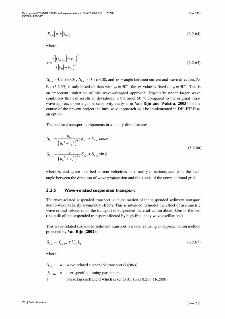
Description of TRANDPOR2004 and Implementation in Delft3D-ONLINE Z3748 May, 2004 INTERIM REPORT
WL | Delft Hydraulics 3 — 2 2
, ,b w b cS r S= (3.2.64)
where:
( )( )
3
,
3
for cr
R cr
U vr
v v
δ −=
−(3.2.65)
, 0b wS = if r<0.01, , 0b cS = if r>100, and ϕ = angle between current and wave direction. As
Eq. (3.2.59) is only based on data with 90ϕ = ° , the ϕ -value is fixed to 90ϕ = ° . This is
an important limitation of this wave-averaged approach. Especially under larger waveconditions this can results in deviations in the order 50 % compared to the original intra-wave approach (see e.g. the sensitivity analysis in Van Rijn and Walstra, 2003). In thecourse of the present project the intra-wave approach will be implemented in DELFT3D asan option.
The bed load transport components in x- and y-direction are:
( )
( )
, , ,0.52 2
, , ,0.52 2
cos
sin
bb x b c b w
b b
bb y b c b w
b b
uS S S
u v
vS S S
u v
φ
φ
= ++
= ++
(3.2.66)
where ub and vb are near-bed current velocities in x- and y-directions, and φ is the local
angle between the direction of wave propagation and the x-axis of the computational grid.
3.2.5 Wave-related suspended transport
The wave-related suspended transport is an estimation of the suspended sediment transportdue to wave velocity asymmetry effects. This is intended to model the effect of asymmetricwave orbital velocities on the transport of suspended material within about 0.5m of the bed(the bulk of the suspended transport affected by high frequency wave oscillations).
This wave-related suspended sediment transport is modelled using an approximation methodproposed by Van Rijn (2002):
, SUSWs w A TS f U Lγ= (3.2.67)
where:
,s wS = wave-related suspended transport (kg/m/s)
SUSWf = user specified tuning parameter
γ = phase lag coefficient which is set to 0.1 (was 0.2 in TR2000)

Description of TRANDPOR2004 and Implementation in Delft3D-ONLINE Z3748 May, 2004 INTERIM REPORT
WL | Delft Hydraulics 3 — 2 3
AU = velocity asymmetry value (m/s) =4 4, ,
3 3, ,
for back
for back
U U
U Uδ δ
δ δ
−
+
TL = suspended sediment load (kg/m2) = 500.007 s ed Mρ
The streaming velocity is not included in the implementation. In Delft3D the streaming isincluded as an additional shear stress distributed linearly across the wave boundary layer(Walstra et al., 2000).
The wave-related suspended transport components in x- and y-directions are:
, , ,
, , ,
cos
sins w x s w
s w y s w
S S
S S
φ
φ
=
=(3.2.68)

Description of TRANDPOR2004 and Implementation in Delft3D-ONLINE Z3748 May, 2004 INTERIM REPORT
WL | Delft Hydraulics 4 — 1
4 Conclusions
4.1 Updated sand transport model TRANSPOR2004 (TR2004)
In Chapter 2 it was shown that the updated transport formulations of TR2004 performedwell in the comparison against over 50 data sets. It was shown that TR2004 was able to givegood to reasonable predictions for most datasets for a range of hydrodynamic and sedimentconditions.
4.2 Sand transport formulations in DELFT3D model
In Chapter 3 a detailed overview is give of the updated formulations in Delft3D-ONLINE.The implementation of TR2004 in Delft3D-ONLINE is part of an update of Delft3D whichinvolves among others: the extension of the model to be run in profile mode, an update ofthe SWAN wave model and the synchronisation of the roughness formulations. The presentreport only describes the implementation of TR2004 formulations in Delft3D-ONLINE. Atthe end of the project this description will be updated to completely describe themodifications and improvements in the final updated version of Delft3D-ONLINE.

Description of TRANDPOR2004 and Implementation in Delft3D-ONLINE Z3748 May, 2004 INTERIM REPORT
WL | Delft Hydraulics 5 — 1
5 References
Andrews, D.G. and Mcintyre, M.E., 1978: An exact theory of non-linear waves on a Lagrangian-mean flow. J.Fluid Mech., Vol. 89 (4), pp. 609-646.
Davies, A.G. and Villaret, C., 1999. Eulerian drift induced by progressive waves above rippled and very roughbed, p. 1465-1488. Journal of Geophysical Research, Vol. 104, No. C1
Delft Hydraulics, 1999. Voortschrijdend Onderzoek Programma (VOP); Generiek kustonderzoek voor de jaren2000-2004. Report Z2478, Delft, The Netherlands
Dingemans, M.W., Radder, A.C. and De Vriend, H.J., 1987. Computation of the Driving Forces of Wave-Induced Currents. Coastal Engineering. 11: 539-563.
Forester, C.K., 1979: Higher Order Monotonic Convective Difference Schemes. Journal of ComputationalPhysics, Vol. 23, 1-22.
Fredsøe, J., 1984. Turbulent boundary layer in wave-current interaction. Journal of Hydraulic Engineering,ASCE, Vol. 110, 1103-1120.
Grasmeijer, B.G., 2002. Process-based cross-shore modelling of barred beaches. Doctoral Thesis, Department ofPhysical Geography, University of Utrecht, Utrecht, The Netherlands
Grasmeijer, B, and Tonnon, P.K., 2003. Preliminary analysis of sand transport measurements at Noordwijksite, North Sea, March-April 2003. Dep. of Physical Geography, University of Utrecht, Utrecht
Grasmeijer, B.T. and Van Rijn, L.C., 1999. Transport of fine sands by currents and waves, Part III: Breakingwaves over barred profile with ripples. Journal of Waterway, Port, Coastal and Ocean Engineering, Vol.125, No. 2
Groeneweg, J. and Klopman, G., 1998. Changes of the mean velocity profiles in the combined wave-currentmotion in a GLM formulation, J. Fluid Mech., Vol 370, pp. 271-296.
Groeneweg, J., 1999. Wave-current interactions in a generalised Lagrangian Mean formulation, PhD thesis,Delft University of Technology, Delft.
Holthuijsen, L.H., N. Booij and T.H.C. Herbers, 1989. A prediction model for stationary, short-crested wavesin shallow water with ambient currents. Coastal Engineering, 13, pp. 23-54.
Holthuijsen, L.H., N. Booij and R.C. Ris, 1993. A spectral wave model for the coastal zone. Proc. of the 2nd
Int. Symposium on Ocean Wave Measurement and Analysis, New Orleans, 630-641.
Huang, W. and Spaulding, M., 1996. Modelling horizontal diffusion with sigma coordinate system, Journal ofHydraulic Eng., Vol. 122, No. 6, 349-352.
Isobe, M. and Horikawa, K., 1982. Study on water particle velocities of shoaling and breaking waves. CoastalEngineering in Japan, Vol. 25.
Jonsson , I.G. and Carlsen, N.A., 1976. Experimental and theoretical investigations in an oscillatory roughturbulent boundary layer. Journal of Hydraulic Research, Vol. 14, No. 1, p. 45-60
Jacobs, C. and Dekker, S., 2000. Sediment concentrations due to currents and irregular waves: the effect ofgrading of the bed material, Measurements Report. Delft University of Technology, Delft, TheNetherlands
Kolmogorov, A. N., 1942. Equations of turbulent motion of an incompressible fluid. IZV Akad. Nauk. USSR,Ser. Phys., Vol. 6, pp. 56-58. (translated into English by D.B. Spalding, as Imperial College,Mechanical Engineering Department Report ON/6, 1968, London, U.K.).
Kroon, A., 1994. Sediment transport and morphodynamics of the beach and nearshore zone near Egmond, TheNetherlands. Doc. Thesis, Dep. of Physical Geography, Univ. of Utrecht, The Netherlands
Leendertse, J.J., 1987. A three-dimensional alternating direction implicit model with iterative fourth orderdissipative non-linear advection terms. WD-333-NETH, The Netherlands Rijkswaterstaat.
Lesser, G. et al., 2003. Development and validation of a three-dimensional morphological model. In press.
Madsen, O.S. et al., 1993. Wind stress, bed roughness and sediment suspension on the inner shelf during anextreme storm event. Continental Shelf Research, Vol. 13, No. 11, pp 1303-1324.
Mellor, G.L. and A.F. Blumberg, 1985. Modelling vertical and horizontal diffusivities and the sigmacoordinate system. Monthly Weather Review, Vol. 113, 1379-1383.

Description of TRANDPOR2004 and Implementation in Delft3D-ONLINE Z3748 May, 2004 INTERIM REPORT
WL | Delft Hydraulics 5 — 2
Prandtl, L., 1945. Uber ein neues formelsystem fur die ausgebildete turbulenz (On a new formation for fullydeveloped turbulence). Nachr. Akad. Wiss. (Report of Academy of Sciences) Gottingen, Germany.
Rodi, W., 1984. Turbulence models and their application in Hydraulics, State-of-the-art paper article sur l’etatde connaissance. Paper presented by the IAHR-Section on Fundamentals of Division II: Experimentaland Mathematical Fluid Dynamics, The Netherlands.
SEDMOC-EU project, 2001. Database sand transport, Delft Hydraulics
Simonin, O., R.E. Uittenbogaard, F. Baron, and P.L. Viollet, 1989. Possibilities and limitations to simulateturbulence fluxes of mass and momentum, measured in a steady stratified mixing layer. In Proc. XXIIIIAHR Congress, Ottawa, August 21-25, published by National Research Council Canada, pp. A55-A62.
Sistermans, P.J.G., 2000. Net sediment transport measurements per fraction for well-graded sediment byirregular waves and a current: data report. Delft University of Technology. Delft. The Netherlands
Sistermans, P.J.G., 2002. Graded sediment transport by non-breaking waves and a current. Doc. Thesis. Dep.of Civil Engineering. Delft University of Technology. Delft. The Netherlands
Stelling, G.S., 1983. On the construction of computational methods for shallow water flow problems. Ph.D. Thesis,Delft Univ. of Techn., Delft.
Stelling, G.S. and Kester, van J.A.T.M., 1994. On the approximation of horizontal gradients in sigmacoordinates for bathymetry with steep bottom slopes. Int. J. Num. Meth. Fluids, Vol. 18, 915-955.
Stelling, G.S. and Leendertse, J.J., 1991. Approximation of Convective Processes by Cyclic ACI methods.Proceeding 2nd ASCE Conference on Estuarine and Coastal Modelling, Tampa.
Stive, M.J.F. and Wind, H.G., 1986. Cross-shore mean flow in the surf zone. Coastal Eng., 10, pp. 235-340.
Svendsen, I.A., 1985. On the formulation of the cross-shore wave-current problem. Proc. Workshop “EuropeanCoastal Zones”. Athens, pp. 1.1-1.9.
Soulsby, R.L., L. Hamm, G. Klopman, D. Myrhaug, R.R. Simons, and G.P. Thomas, 1993. Wave-currentinteraction within and outside the bottom boundary layer. Coastal Engineering, 21 (1993) 41-69,Elsevier Science Publishers B.V., Amsterdam.
Uittenbogaard, R.E., 1998. Model for eddy diffusivity and viscosity related to sub-grid velocity and bedtopography. Note, WL | Delft Hydraulics.
Van Ledden, M., 2003. Sand-mud segregation in estuaries and tidal basins. Doctoral Thesis, Civil EngineeringDepartment, Delft University of Technology , Delft, The Netherlands
Van Rijn, L.C., 1993. Principles of sediment transport in rivers, estuaries and coastal seas. Aqua Publications,The Netherlands
Van Rijn, L.C., 2000. General view on sand transport by currents and waves, Report Z2899.20-Z2099.30-Z2824.30, Delft Hydraulics, Delft, The Netherlands
Van Rijn, L.C., 2002. Approximation formulae for sand transport by currents and waves and implementation inDELFT-MOR. Report Z3054.20, Delft Hydraulics, Delft, The Netherlands.
Van Rijn, L.C., 2003. Sand Transport by currents and waves; general approximation formulae. CoastalSediments 1999, ASCE, Long Island New York.
Van Rijn, L.C. and Walstra, D.J.R., 2003. Modelling of Sand Transport in Delft3D, WL | Delft Hydraulicsreport Z3624.
Van Vossen, B., 2000. Horizontal Large Eddy Simulations; evaluation of computations with DELFT3D-FLOW.Report MEAH-197, Delft University of Technology.
Verboom, G.K. and Slob, A., 1984. Weakly reflective boundary conditions for two-dimensional water flowproblems. 5th Int. Conf. on Finite Elements in Water Resources, June 1984, Vermont. Also Adv. WaterResources, Vol. 7, December 1984, Delft Hydraulics publication No. 322.
Walstra, D.J.R., J.A. Roelvink and J. Groeneweg, 2000: Calculation of wave-driven currents in a 3D meanflow model. In: Coastal Engineering 2000, Billy Edge (ed.), Vol. 2, ASCE, New York, pp. 1050-1063.
Whitehouse, R.J. et al., 1996. Sediment transport measurements at Maplin Sands, Outer Thames Estuary.Report TR 15, HR Wallingford, England
Whitehouse, R.J. et al., 1997. Sediment transport measurements at Boscombe Pier, Poole Bay. Report TR 27,HR Wallingford, England
Wolf, F.C.,J., 1997. Hydrodynamics, sediment transport and daily morphological development of a bar-beachsystem. Doc. Thesis, Dep. of Physical Geography, Univ. of Utrecht, The Netherlands

Description of TRANDPOR2004 and Implementation in Delft3D-ONLINE Z3748 May, 2004 INTERIM REPORT
WL | Delft Hydraulics 5 — 3

Description of TRANDPOR2004 and Implementation in Delft3D-ONLINE Z3748 May, 2004 INTERIM REPORT
WL | Delft Hydraulics A – 1
A TRANSPOR2004-MODEL; computation of bed forms, bed roughness and sand transport in combined currents and waves

Description of TRANDPOR2004 and Implementation in Delft3D-ONLINE Z3748 May, 2004 INTERIM REPORT
WL | Delft Hydraulics A – 2
1. InputParameter Description dimensionh Water depth mvR Depth-averaged velocity vector in main flow direction
(see Figure A.1)m/s
ur Time- and depth-averaged return velocity below wave troughcompensating the mass transport between wave crest and wavetrough (- in backward or offshore direction)(see Figure A.1); ur is defined with respect to the wavedirection; ur is always negative (against the wave direction)
m/s
Hs Significant wave height mTP Period of peak of wave spectrum s
ϕ Angle between wave and main flow direction (0 to 360o) -
N Number of sand fractions -di; pi If N>1;fraction diameter and fraction percentage (∑pi=1)
(N>1 multi-fraction method)m
d10 If N=1; sand diameter exceeded by 90% of total sample(single fraction method)
m
d50 If N=1; median sand diameter md90 If N=1; sand diameter exceeded by 10% of total sample mpmud Fraction of mud (<0.05 mm) in sample of bed material
(pmud in range of 0. to 0.3)-
Type of bedroughness
Selection parameter(1 for rivers; 2 for estuaries; 3 for seas)
-
FACR Linear scaling factor for bed roughness height (default=1) -Te Water temperature CelsiusSa Salinity Promille
Figure A.1 Schematic presentation of current and wave direction
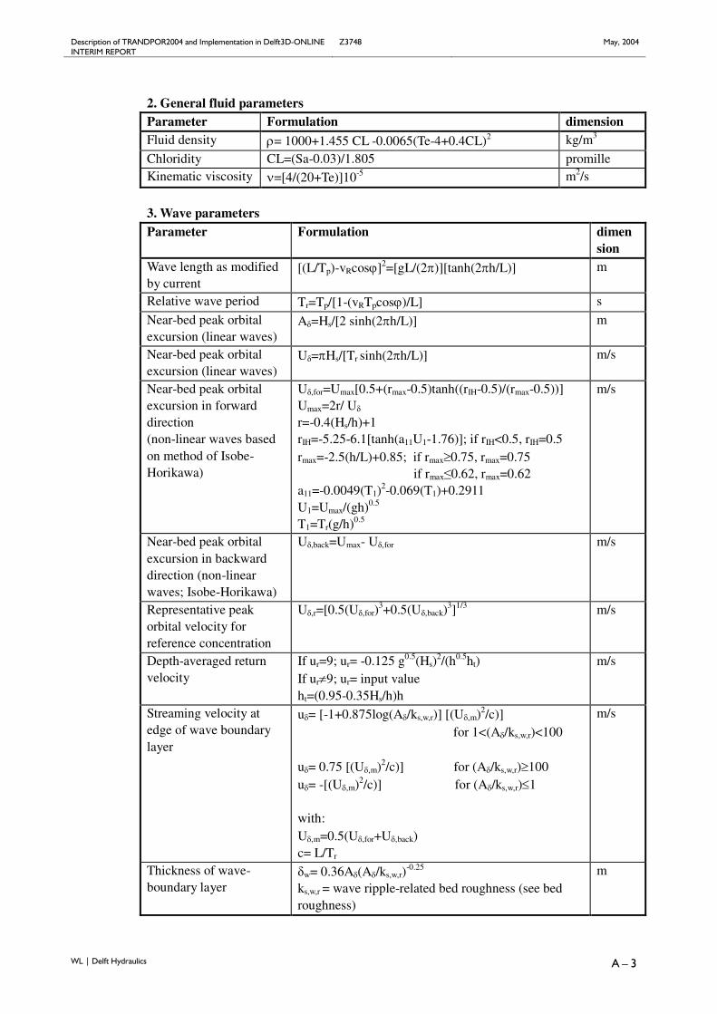
Description of TRANDPOR2004 and Implementation in Delft3D-ONLINE Z3748 May, 2004 INTERIM REPORT
WL | Delft Hydraulics A – 3
2. General fluid parametersParameter Formulation dimensionFluid density ρ= 1000+1.455 CL -0.0065(Te-4+0.4CL)2 kg/m3
Chloridity CL=(Sa-0.03)/1.805 promilleKinematic viscosity ν=[4/(20+Te)]10-5 m2/s
3. Wave parametersParameter Formulation dimen
sionWave length as modifiedby current
[(L/Tp)-vRcosϕ]2=[gL/(2π)][tanh(2πh/L)] m
Relative wave period Tr=Tp/[1-(vRTpcosϕ)/L] s
Near-bed peak orbitalexcursion (linear waves)
Aδ=Hs/[2 sinh(2πh/L)] m
Near-bed peak orbitalexcursion (linear waves)
Uδ=πHs/[Tr sinh(2πh/L)] m/s
Near-bed peak orbitalexcursion in forwarddirection(non-linear waves basedon method of Isobe-Horikawa)
Uδ,for=Umax[0.5+(rmax-0.5)tanh((rIH-0.5)/(rmax-0.5))]Umax=2r/ Uδ
r=-0.4(Hs/h)+1rIH=-5.25-6.1[tanh(a11U1-1.76)]; if rIH<0.5, rIH=0.5rmax=-2.5(h/L)+0.85; if rmax≥0.75, rmax=0.75
if rmax≤0.62, rmax=0.62a11=-0.0049(T1)
2-0.069(T1)+0.2911U1=Umax/(gh)0.5
T1=Tr(g/h)0.5
m/s
Near-bed peak orbitalexcursion in backwarddirection (non-linearwaves; Isobe-Horikawa)
Uδ,back=Umax- Uδ,for m/s
Representative peakorbital velocity forreference concentration
Uδ,r=[0.5(Uδ,for)3+0.5(Uδ,back)
3]1/3 m/s
Depth-averaged returnvelocity
If ur=9; ur= -0.125 g0.5(Hs)2/(h0.5ht)
If ur≠9; ur= input valueht=(0.95-0.35Hs/h)h
m/s
Streaming velocity atedge of wave boundarylayer
uδ= [-1+0.875log(Aδ/ks,w,r)] [(Uδ,m)2/c)]for 1<(Aδ/ks,w,r)<100
uδ= 0.75 [(Uδ,m)2/c)] for (Aδ/ks,w,r)≥100uδ= -[(Uδ,m)2/c)] for (Aδ/ks,w,r)≤1
with:Uδ,m=0.5(Uδ,for+Uδ,back)c= L/Tr
m/s
Thickness of wave-boundary layer
δw= 0.36Aδ(Aδ/ks,w,r)-0.25
ks,w,r = wave ripple-related bed roughness (see bedroughness)
m

Description of TRANDPOR2004 and Implementation in Delft3D-ONLINE Z3748 May, 2004 INTERIM REPORT
WL | Delft Hydraulics A – 4
Thickness of effectivefluid mixing layer
δm=2 δw
δm,min=0.05; δm,max=0.2m
4. Current vectorParameter Formulation dimensionOverall currentvector
VR=[vR2 + ur
2 + 2 vR ur cosϕ]0.5 m/s
5. Sediment characteristics (single fraction method)Parameter Formulation dimensionRelative density s=ρs/ρ -
Particle sizes Single fraction methodd10, d50 and d90 (input values)Multi-fraction methodd10, d50 and d90 computed from fraction sizes andpercentages
Particle parameter D*=d50[(s-1)g/ν2]1/3 ; Single fraction method
D*,i=di[(s-1)g/ν2]1/3 ; Multi-fraction method
-
Initiation of motion θcr=0.115 (D*)-0.5 for 1< D*≤4
θcr=0.140 (D*)-0.64 for 4< D*≤10
θcr=0.040 (D*)-0.1 for 10< D*≤20
θcr=0.013 (D*)0.29 for 20< D*≤150
θcr=0.055 for D*>150
-
Critical bed-shearstress
τcr=(ρs-ρ) g d50 θcr
τcr,1=(1+pmud)3(ρs-ρ) g d50 θcr
N/m2
Critical depth-averaged velocity
ucr=5.75[(s-1)gd50]0.5(θcr)
0.5log(4h/d90) m/s
Critical peak orbitalvelocity (Komar)
Ucr=[0.12(s-1)g(d50)0.5 (Tp)
0.5]2/3 for d50<0.0005 mUcr=[1.09(s-1)g(d50)
0.75 (Tp)0.25]0.571 for d50≥0.0005 m
m/s
Mobility parameter ψ=(Uwc)2/((s-1)gd50))
Uwc= [(Uδ,r + |ur|)2 + (vR)2 + 2(Uδ,r+|ur|)(vR)cosφ]0.5
-
Suspended sandsize
ds= min[0.5d50,(1+0.0006(d50/d10-1)(ψ-550))d50]for ψ<250
ds=d50 for ψ≥250
m
Fall velocity Single fraction methodws is computed by using Equation (3.2.22) based onds;
Multi-fraction methodws,i is computed by using similar expressions basedon di
m/s

Description of TRANDPOR2004 and Implementation in Delft3D-ONLINE Z3748 May, 2004 INTERIM REPORT
WL | Delft Hydraulics A – 5
6. Bed roughnessParameter Formulation dimen
sionOverall current-related bedroughness
ks,c=FACR [(ks,c,r)2 + (ks,c,mr)
2 + (ks,c,d)2]0.5
FACR=input value (default=1)
m
Current-relatedbed roughnessdue to ripples
ks,c,r=150d50 for ψ≤50ks,c,r=20d50 for ψ≥250ks,c,r=(182.5-0.65ψ)d50 for 50<ψ<250ks,c,r,max=0.075
m
Current-relatedbed roughnessdue to mega-ripples
ks,c,mr=0.01 h for ψ≤50, h>1 and vR>0.3ks,c,mr=0 for ψ≥550, h>1 and vR>0.3ks,c,mr=(0.011-0.00002ψ) h for 50<ψ<550, h>1 and vR>0.3ks,c,mr,max=0.2
m
Current-relatedbed roughnessdue to dunes(only rivers)
ks,c,d=(0.0004ψ)h for Hs=0, ψ≤100, h>1, vR>0.3ks,c,d=0 for Hs=0, ψ≥600, h>1, vR>0.3ks,c,d=(0.048-0.00008ψ) h for Hs=0, 100<ψ<600, h>1, vR>0.3ks,c,d,max=1.0
m
Wave-relatedbed roughnessdue to ripples
ks,w,r=150d50 for ψ≤50ks,w,r=20d50 for ψ≥250ks,w,r=(182.5-0.65ψ)d50 for 50<ψ<250ks,w,r,max=0.075
m
Apparent bedroughness
ka=ks,cexp[γUδ,r/VR]ka,max=10ks,c
γ=0.8+β-0.3β2
β=(ϕ/360)2π; if β>π; β=2π-(ϕ/180) π
m
7. Friction factorsParameter Formulation dimen
sionGrain-relatedChezy coefficient(current-related)
C/=18 log(12h/d90) m0.5/s
Overall Chezycoefficient(current-related)
C=18 log(12h/ks,c) m0.5/s
Grain-relatedfriction factor(current-related)
f/c=0.24[log(12h/d90)]
-2 -
Overall frictionfactor coefficient(current-related)
fc=0.24[log(12h/ks,c)]-2 -
Apparent frictionfactor coefficient
fa=0.24[log(12h/ka]-2 -

Description of TRANDPOR2004 and Implementation in Delft3D-ONLINE Z3748 May, 2004 INTERIM REPORT
WL | Delft Hydraulics A – 6
(current-related)Grain-relatedfriction factor(wave-related)
f/w=exp[-6+5.2(Aδ/d90)
-0.19]f/
w,max=0.05-
Overall frictionfactor coefficient(wave-related)
fw=exp[-6+5.2(Aδ/ks,w,r)-0.19]
fw,max=0.3-
8. Time-averaged bed-shear stressesParameter Formulation dimen
sionEfficiency factor(current-related)
µc= f/c/ fc -
Efficiency factor(wave-related)
Single fraction methodµw= 0.7/D*
µw,min=0.14 for D*≥5µw,max=0.35 for D*≤2
Multi-fraction methodµw,i= 0.7/D*,i
µw,min=0.14 for D*,i≥5µw,max=0.35 for D*,i≤2
-
Wave-currentinteractioncoefficient
αcw=[ln(30δm/ka)/ln(30δm/ks,c)]2
[(-1+ln(30h/ks,c))/(-1+ln(30h/ka))]2
αcw,max=1
-
Bed-shear stresscurrent
τb,c=0.125 ρ fc (VR)2 N/m2
Bed-shear stresswaves
τb,w=0.25 ρ fw (Uδ,w,r)2 N/m2
Bed-shear stresscurrent+waves
τb,cw=αcw τb,c+ τb,w N/m2
Effective bed-shearstress current+waves
τ/b,cw=αcw µc τb,c+µw τb,w; Single fraction method
τ/b,cw,i=αcw µc τb,c+µw,i τb,w; Multi-fraction method
N/m2
Effective bed-shearvelocity current+waves
u/*,cw=(τ/
b,cw/ρ)0.5; Single fraction method
u/*,cw,i=(τ/
b,cw,i/ρ)0.5; Multi-fraction method
m/s
9. Dimensionless bed-shear stress parametersParameter Formulation dimen
sionDimensionless bed-shear stressparameter(current and waves)
Single fraction methodTcw=[τ/
b,cw - τcr,1]/ τcr
Multi-fraction methodTcw,i=λi[τ/
b,cw,i- (τcr,1)(di/d50)ξi]/ [τcr(di/d50)]
-
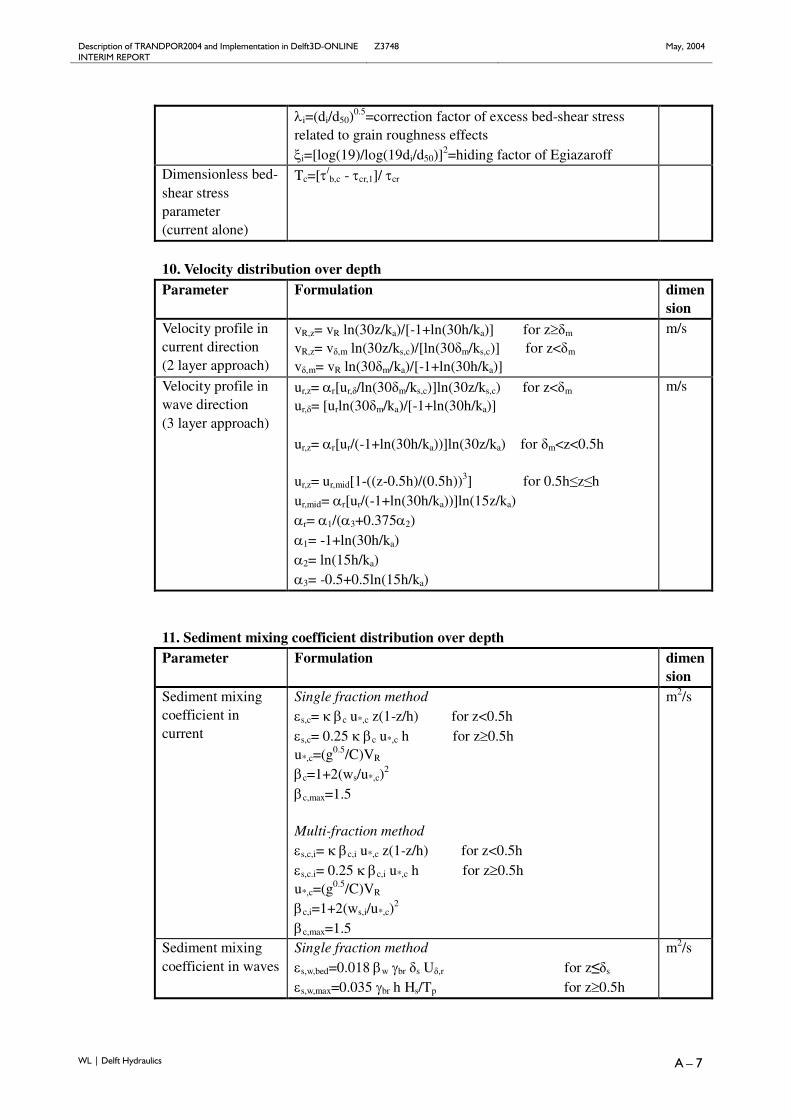
Description of TRANDPOR2004 and Implementation in Delft3D-ONLINE Z3748 May, 2004 INTERIM REPORT
WL | Delft Hydraulics A – 7
λi=(di/d50)0.5=correction factor of excess bed-shear stress
related to grain roughness effectsξi=[log(19)/log(19di/d50)]
2=hiding factor of EgiazaroffDimensionless bed-shear stressparameter(current alone)
Tc=[τ/b,c - τcr,1]/ τcr
10. Velocity distribution over depthParameter Formulation dimen
sionVelocity profile incurrent direction(2 layer approach)
vR,z= vR ln(30z/ka)/[-1+ln(30h/ka)] for z≥δm
vR,z= vδ,m ln(30z/ks,c)/[ln(30δm/ks,c)] for z<δm
vδ,m= vR ln(30δm/ka)/[-1+ln(30h/ka)]
m/s
Velocity profile inwave direction(3 layer approach)
ur,z= αr[ur,δ/ln(30δm/ks,c)]ln(30z/ks,c) for z<δm
ur,δ= [urln(30δm/ka)/[-1+ln(30h/ka)]
ur,z= αr[ur/(-1+ln(30h/ka))]ln(30z/ka) for δm<z<0.5h
ur,z= ur,mid[1-((z-0.5h)/(0.5h))3] for 0.5h≤z≤hur,mid= αr[ur/(-1+ln(30h/ka))]ln(15z/ka)αr= α1/(α3+0.375α2)α1= -1+ln(30h/ka)α2= ln(15h/ka)α3= -0.5+0.5ln(15h/ka)
m/s
11. Sediment mixing coefficient distribution over depthParameter Formulation dimen
sionSediment mixingcoefficient incurrent
Single fraction methodεs,c= κ βc u*,c z(1-z/h) for z<0.5hεs,c= 0.25 κ βc u*,c h for z≥0.5hu*,c=(g0.5/C)VR
βc=1+2(ws/u*,c)2
βc,max=1.5
Multi-fraction methodεs,c,i= κ βc,i u*,c z(1-z/h) for z<0.5hεs,c.i= 0.25 κ βc,i u*,c h for z≥0.5hu*,c=(g0.5/C)VR
βc,i=1+2(ws,i/u*,c)2
βc,max=1.5
m2/s
Sediment mixingcoefficient in waves
Single fraction methodεs,w,bed=0.018 βw γbr δs Uδ,r for z≤δs
εs,w,max=0.035 γbr h Hs/Tp for z≥0.5h
m2/s

Description of TRANDPOR2004 and Implementation in Delft3D-ONLINE Z3748 May, 2004 INTERIM REPORT
WL | Delft Hydraulics A – 8
εs,w=εs,w,bed + [εs,w,max - εs,w,bed][(z-δs)/(0.5h-δs)] for δs<z<0.5hδs=2γbrδw with: δs,min=0.05; δs,max=0.2γbr=1+[(Hs/h)-0.4]0.5 with: γbr=1 for Hs/h<0.4βw=1+2(ws/u*,w)2
βw,max=1.5u*,w=(τb,w/ρ)0.5
Multi-fraction methodεs,w,bed,i=0.018 βw,i γbr δs Uδ,r for z≤δs
βw,i=1+2(ws,i/u*,w)2
Sediment mixingcoefficient incurrent+waves
εs,cw=[(εs,c)2+(εs,w)2]0.5 m2/s
12. Concentration profile over depth by numerical integrationParameter Formulation dimen
sionReference level a=maximum(0.5ks,c,r; 0.5ks,w,r; 0.01) mReferenceconcentration
Single fraction methodca=0.015 (1-pmud) (d50/a) (Tcw)1.5/(D*)
0.3
ca,max=0.05
Multi-fraction methodca,i=0.015 pi (di/a) (Tcw,i)
1.5/(D*,i)0.3
ca,max,i=0.05ca= ∑ca,i (with pmud+∑pi=1)
-
Concentrationgradient
Single fraction methoddc/dz= -[1-c)5c ws]/[βd εs,cw]βd=1+(c/cmax)
0.8-2(c/cmax)0.4
cmax=0.65
Multi-fraction methoddci/dz= -[1-ci)
5ci ws,i]/[βd,i εs,cw,i]βd,i=1+(ci/cmax)
0.8-2(ci/cmax)0.4
cmax=0.65
m-1
13. Time-averaged current-related suspended transport ratesParameter Formulation dimen
sionCurrent direction qs,c1=ρs a∫h (vR,zcz,i)dz; Single fraction method
qs,c1,i=pi ρs a∫h (vR,zcz,i)dz; Multi-fraction methodqs,c1= ∑qs,c1,i
kg/s/m
Wave direction qs,c2=ρs a∫h (ur,zcz)dz; single fraction methodqs,c2,i=pi ρs a∫h (ur,zcz,i)dz; Multi-fraction methodqs,c2= ∑qs,c2,i
kg/s/m

Description of TRANDPOR2004 and Implementation in Delft3D-ONLINE Z3748 May, 2004 INTERIM REPORT
WL | Delft Hydraulics A – 9
14. Time-averaged wave-related suspended transport rateParameter Formulation dimen
sionWave direction qs,w=ρs F a∫0.5 (cz)dz; Single fraction method
F=0.1(Uasym+uδ]Uasym =[(Uδ,for)
4-(Uδ,back)4]/[(Uδ,for)
3 +(Uδ,back)3]
qs,w,i=piρs F a∫0.5 (cz,i)dz; Multi-fraction methodqs,w=∑qs,w,i
kg/s/m
15. Instantaneous and time-averaged bed-load transport rate(x-axis along current velocity vector; see Fig. A.2)(y-axis normal to current velocity vector; see Fig. A.2)
Parameter Formulation dimension
Instantaneousvelocity vector nearbed at z= δ
Vδ =[(vR, δ)2 + (ur, δ)
2 + 2(vR, δ)(ur, δ)cosϕ]0.5 m/s
Forward orbitalvelocities near bed
Uδ,t= Uδ,forsin(πt/Tfor) for t≤Tfor m/s
Backward orbitalvelocities near bed
Uδ,t= -Uδ,backsin(π(t-Tfor)/Tback)) for Tfor<t≤Tback m/s
Instantaneousvelocity in x-direction (current-direction)
Uδ,cw,x,t= vR, δ + ur,δcosϕ + Uδ,tcosϕ + uδcosϕ m/s
Instantaneousvelocity in y-direction
Uδ,cw,y,t= ur,δsinϕ + Uδ,tsinϕ + uδsinϕ m/s
Instantaneousvelocity vector
Uvec,t= [(Uδ,cw,x,t)2 + (Uδ,cw,y,t)
2]0.5 m/s
Friction coefficient f/cw= αv βf f/
c + [1-(αv)0.5]f/
w
αv=|Vδ|/[|Vδ|+|Uδ|]βf=0.25[-1+ln(30h/ks,c)]
2/[ln(30δm/ks,c)]2
-
Instantaneousgrain-related bed-shear stress andbed-shear velocity
τ/b,cw,t=0.5 ρ f/
cw (Uvec,t)2
u/*,cw,t=(τ/
b,cw,t/ρ)0.5
N/m2
m/s
Instantaneous bed-shear stressparameter
Single fraction methodTcw,t=[τ/
b,cw,t - fslope2 τcr,1]/τcr
fslope2=sin[atan(0.6)+atan(βslope)]/sin[atan(0.6)]βslope=βslope,x(Ux,t/Uvec,t) + βslope,y(Uy,t/Uvec,t)βslope,x=0 (bed slope in x-direction)βslope,y=0 (bed slope in y-direction)Multi-fraction methodTcw,t,i=λi[τ/
b,cw,t - fslope2 (di/d50)ξi τcr,1]/[τcr(di/d50)]
-
Instantaneous bed- Single fraction method kg/s/m

Description of TRANDPOR2004 and Implementation in Delft3D-ONLINE Z3748 May, 2004 INTERIM REPORT
WL | Delft Hydraulics A – 1 0
load transportvector
qb,t=0.5 (1-pmud) ρs fslope1 d50 u/*,cw,t Tcw,t/(D*)
0.3
fslope1=1/[1+βslope/0.6]Multi-fraction methodqb,t,i=0.5 pi ρs fslope1 di u/
*,cw,t Tcw,t.i/(D*,i)0.3
Instantaneous bed-load transport ratein x- and y-directions
Single fraction methodqb,t,x=(Ux,t/Uvec,t) qb,t
qb,t,y=(Uy,t/Uvec,t) qb,t
kg/s/m
Time-averaged bed-load transportvector andcomponents incurrent and wavedirections
<qb>= (1/Tp)[(∑qb,t,x)2 + (∑qb,t,y)
2]0.5
<qb,c>=((1/Tp)[∑(qb,t,x)- (1/tanϕ)(∑(qb,t,y)]<qb,w>=(1/Tp)∑(qb,t,y)/sinϕMulti-fraction methodqb,t,x,i=(Ux,t/Uvec,t) qb,t,i
qb,t,y,i=(Uy,t/Uvec,t) qb,t,i
<qb>=∑N (1/Tp) [(∑qb,t,x,i)2 + (∑qb,t,y,i)
2]0.5
<qb,c>=∑N (1/Tp) [∑(qb,t,x,i)- (1/tanϕ)(∑(qb,t,y,i)]<qb,w>=∑N (1/Tp) ∑(qb,t,y,i)/sinϕ
kg/s/m
16. Time-averaged total load transport ratesParameter Formulation dimen
sionCurrent direction qt,c=qs,c1 + <qb,c> kg/s/mWave direction qt,w=qs,c2 + qs,w + <qb,w> kg/s/m

Description of TRANDPOR2004 and Implementation in Delft3D-ONLINE Z3748 May, 2004 INTERIM REPORT
WL | Delft Hydraulics A – 1 1
Figure A.2 Instantaneous velocity vector near bed (at z=δm)
17. Bed form dimensionsType ofbed forms
Formulation(∆=λ=0 outside validity ranges)
dimension
Ripples inrivers
∆r=100d50; if Hs<0.01 and D*<10 and Tc<25λr=750d50
m
Mega-ripples inrivers
∆mr= 0.02h(10-Tc)(1-e-0.1Tc) if Hs<0.01 and D*<10 and 1≤Tc<10λmr=0.5h
m
Dunes inrivers
∆d= 0.11h(d50/h)0.3(25-Tc)(1-e-0.5Tc) if Hs<0.01 and 1≤Tc<25λd=7.3h
m
Sand wavesin rivers
∆sw= 0.15h (1-Fr2)(1-e-0.5(Tc-15) ) if Hs<0.01, Tc≥15, Fr<0.8 and h≥1λsw=10h
m
Ripples inestuaries
∆r=100d50; if Hs<0.01 and D*<10 and Tcw<25λr=750d50
m
Mega-ripples inrestuaries
∆mr= 0.02h(10-Tcw)(1-e-0.1Tcw) if Hs<0.01, D*<10, 1≤Tcw<10 and h≥1λmr=0.5h
m
Dunes inestuaries
∆d= 0.05h if Hs<0.01 and 1≤Tcw<25 and h≥1λd=2h
m

Description of TRANDPOR2004 and Implementation in Delft3D-ONLINE Z3748 May, 2004 INTERIM REPORT
WL | Delft Hydraulics A – 1 2
Sand wavesin estuaries
∆sw= 0.05h if Hs<0.01, Tcw≥15, Fr<0.8 and h≥1λd=3h
m
Ripples incoastal seas
∆r=0.22 Aδ if Hs≥0.01 and ψ<10λr=5.6∆r
∆r=2.8 10-13 (250-ψ)5 Aδ if Hs≥0.01 and 10≤ψ<250λr=∆r/[2 10-7(250-ψ)2.5]
m
Mega-ripples incoastal seas
∆mr=0.02 h if Hs≥0.01 and ψ<550 and h≥1 and vR≥0.3λmr=0.5 h
m
Sand wavesin coastalseas
∆sw=0.1 h if Hs≥0.01 and h≥10 and vR≥0.5λsw=10 h
m