DOES MONEYMATTER IN THEEURO AREA?EVIDENCE FROM ANEW DIVISIA INDEXZSOLT DARVAS

Highlights • Standard simple-sum monetary aggregates, like M3, sum up monetary

assets that are imperfect substitutes and provide different transactionand investment services. Divisia monetary aggregates, originated fromBarnett (1980), are derived from economic aggregation and indexnumber theory and aim to aggregate the money components byconsidering their transaction service.

• No Divisia monetary aggregates are published for the euro area, incontrast to the United Kingdom and United States. We derive and makeavailable a dataset on euro-area Divisia money aggregates for January2001 – February 2015 using monthly data. We plan to update thedataset in the future.

• Using structural vector-autoregressions, we find that Divisia aggregateshave significant impacts on euro-area output and prices. Following ashort-term liquidity effect, Divisia-money shocks tend to increaseinterest rates, suggesting that the European Central Bank reacts todevelopments in monetary aggregates. Divisia-money declines after ashock to user cost, consistently with a money-demand function, whilean interest rate shock increases user cost and decreases Divisia-money, suggesting that the ECB can influence monetary developments.Most of these results are not significant when we use simple-summeasures of money.

• Our findings complement the evidence from US data that Divisiamonetary aggregates are useful in assessing the impacts of monetarypolicy and that they work better in SVAR models than simple-summeasures of money.

Zsolt Darvas (zsolt.darvas@bruegel.org) is a Senior Fellow at Bruegel. Theauthor is grateful to Barry E. Jones for a discussion on Divisia calculationsand for suggesting the use of ECB transactions data, to an anonymousreviewer, Bruegel colleagues and participants at the 3rd EuropeanConference on Banking and the Economy (ECOBATE 2014) for commentsand suggestion, and to Pia Hüttl and Thomas Walsh for researchassistance.

BRUE

GEL

WOR

KING

PAP

ER 20

14/1

2

NOVEMBER 2014(UPDATED APRIL 2015)

1. Introduction

Money has a minor role in monetary policy and macroeconomic modelling. One important cause for this

disregard is empirical: estimated money demand functions have been found to be unstable and money has

proved to be less effective in predicting economic outcomes1. However, such empirical failures are challenged

by the literature on aggregation-theoretic measurement of money. The most widely used measures of money,

like M2 and M3, are simple-sum measures. Simple-sum aggregation implies that all components of the money

stock are perfect substitutes, which is a very restrictive and improbable assumption. Correct aggregation can be

obtained by using either aggregation theory or index number theory, as first underlined by Barnett (1980), who

suggested the discrete-time Törnquist-Theil approximation of the Divisia index.

Recent studies using US data also underlined the usefulness of Divisia money indicators for monetary analysis.

Within a cointegrated vector-autoregressive model, Hendrickson (2013) identified a stable money demand

equation using Divisia indicators and demonstrated that they Granger-cause the growth and level of output and

the level of prices. The same analyses with simple-sum money indicators led to weaker results. Keating et al

(2014) showed that a structural vector-autoregressive (SVAR) model with Divisia money worked as well as the

model with the Federal funds rate before the crisis. It worked equally well in the sample period that includes the

zero lower bound when the Federal funds rate model could not be used. Using a different SVAR model, Belongia

and Ireland (2014) found support for the inclusion of Divisia money in the US monetary policy rule and also

identified reasonable money demand and monetary system shocks.

Our paper creates a new dataset on euro-area Divisia money aggregates and examines the impacts of shocks to

money, money user cost and interest rate on output, prices and monetary variables in the euro area, using SVAR

models.

2. A new euro-area Divisia money dataset

No Divisia monetary aggregates are available for the euro area, in contrast to the US and UK2. We create and

make available a dataset on euro-area Divisia aggregates corresponding to the simple-sum aggregates

published by the European Central Bank (ECB), ie M1, M2 and M3, for January 2001 – February 2015. We plan

to update the dataset in the future3.

Earlier academic works on the euro-area Divisia aggregates include Wesche (1997), Reimers (2002), Stracca

(2004), Barnett (2007), Binner et al (2009), Jones and Stracca (2012) and Barnett and Gaekwad-Babulal

(2014). In contrast to most of these papers, we base our calculations on euro-area data as opposed to

aggregating country-specific data at the euro-area level. Furthermore, instead of relying on an ad-hoc spread

1 Other reasons were policy shifts by central banks to focus on interest rates and the development of theories suggesting that money is redundant, see Leeper and Roush (2003), Belongia and Ireland (2014), Keating et al (2014). 2 Divisia indices are published by the Center of Financial Stability (CFS) and the Federal Reserve Bank of St. Louis for the US and the Bank of England for the UK. 3 Our dataset is downloadable from: http://www.bruegel.org/datasets/divisia-dataset/

2

assumption to approximate the benchmark rate (the return on a monetary asset that does not provide

transaction services), as generally done in the literature, we derive it by considering longer maturity bank debts.

The ECB indicators of euro-area outstanding money stocks are subject to two major shortcomings. First, they

relate to the changing country-composition euro-area and hence there was a level shift in these indicators

whenever a new member joined the euro area. Second, they are subject to reclassification changes, such as

halving the outstanding stock of the measure of repurchase agreements in June 2010. For economic analysis,

such level shifts should be eliminated. We create a Divisia index for the first twelve euro-area members based

on transactions data, which does not suffer from level shift problems. Details are provided in the online

Appendix.

3. Models and data

We estimate impulse response functions with SVAR models including five variables: GDP, GDP deflator, money,

the user cost of money and interest rate. The sample period is quarterly between 2001Q1 and 2014Q4, which is

shorter than sample periods available for the US, so we are obliged to use relatively small-scale models and

cannot study sub-sample stability4. Output, prices and money enter the model in log-levels, while the interest

rate and user cost are included in percent. Such a specification leads to consistent estimation, irrespective of

whether or not there is a co-integration relationship between the variables.

For GDP and GDP deflator we use the seasonally adjusted euro-area twelve (i.e. constant country composition)

aggregates published by Eurostat.

For money, we use seasonally adjusted end-of-quarter M2 data from our new dataset (results with M3 are very

similar). We compare the results obtained with Divisia and simple-sum measures. To facilitate the comparison,

we calculate the simple-sum measure for the first twelve euro-members using transactions data to exclude

level shifts, similarly to the Divisia-index.

The user cost of a monetary asset is the function of the interest forgone by holding that asset rather than the

benchmark asset. Thereby, a higher user cost reduces the demand for that asset. Note that the impact of a

higher interest rate on the demand for monetary assets (other than the zero-yielding cash) is ambiguous,

because, for example, a higher central bank interest rate may increase the interest rate paid on deposits, which

in itself makes deposits more attractive.

For the interest rate we use the 10-year maturity German government bond yield, because the ECB policy rate or

a measure of short-term interest rate cannot be used due to reaching zero lower bound in the latter part of our

sample period. The expectation hypothesis of the term structure of interest rates defines the relationship

between current and expected short-term interest rates and the long-term interest rate. Thereby, the long-term

rate can be informative about monetary policy actions, including when various unconventional measures, such 4 We allow four lags in the VARs, which reduces our effective sample period by 4 to 52. We need to estimate 21 parameters per equation (four lags of each of the five variables plus an intercept), which leaves reasonable degrees of freedom.

3

as large-scale asset purchases, are implemented. We use the German rate and not the euro-area average,

because the average was influenced by redenomination risk during the euro-area sovereign debt crisis, while

the German rate is the closest to a euro-area risk-free asset.

Our relatively short sample period does not allow a rich identification of structural shocks. We therefore use the

generalised impulse response function derived by Pesaran and Shin (1998), which does not depend on the

variable ordering, in contrast to the Cholesky-decomposition. Thereby we cannot interpret any of our shock as a

‘monetary policy shock’, yet shocks to the interest rate may capture most of such shocks. A shock to user cost

is not a pure money demand shocks, but may approximate it, while a shock to money may comprise money

supply shocks.

4. Results

Figure 1 shows that the response of output to a Divisia-money shock is positive and statistically significant

about 3-9 quarters after the shock, which corresponds to the horizon at which monetary policy is thought to

have an effect on the economy. The output level response is temporary as the impulse-response function

returns to zero, which is sensible and in line with the long-run neutrality hypothesis. While the shape of the

response to a simple-sum money shock is similar, it is significant for a shorter period (3-6 quarters).

The price response is marginally significant for the Divisia aggregate, but not significant for the simple-sum

aggregate. The point estimates suggest that prices increase after a money shock, which is sensible. The price

response to the interest rate is negative, as expected, and is significant in the Divisia- model, but not in the

simple-sum model.

The interest rate decreases significantly in the short-term after a Divisia money shock and thereby no liquidity

puzzle arises. When simple-sum money is used, the short-term impact is not significant. Starting from about a

year after the money shock, the interest rate response turns to positive, which is significant for both measures

of money. To the extent that the long-term interest rate reflects ECB monetary actions, this finding suggests that

the ECB reacted to monetary developments, e.g. by cutting its policy rate or by adopting unconventional

monetary measures following a negative money shock.

A shock to user cost reduces money, which is consistent with a money-demand function. This effect is

significant for up to three years after the shock in the Divisia-model and for less than two years in the simple-

sum model.

Finally, in the Divisia-model an interest rate shock increases the user cost of money, which may explain why the

reaction of money is negative to an interest rate shock. These findings imply that the ECB can influence money

growth by impacting long-term interest rates. However, these findings do not hold in the simple-sum model, as

4

the impacts of an interest rate shock on user cost and money are not significant and even the point estimates

are virtually zero5.

Figure 1: Impulse responses to interest rate and money shocks

A: Using M2 Divisia

-.012

-.008

-.004

.000

.004

.008

.012

.016

5 10 15 20-.012

-.008

-.004

.000

.004

.008

.012

.016

5 10 15 20-.012

-.008

-.004

.000

.004

.008

.012

.016

5 10 15 20

-.004

-.002

.000

.002

.004

5 10 15 20

Shock to money

-.004

-.002

.000

.002

.004

5 10 15 20

Shock to user cost Shock to interest rate

-.004

-.002

.000

.002

.004

5 10 15 20

-.012

-.008

-.004

.000

.004

.008

.012

5 10 15 20-.012

-.008

-.004

.000

.004

.008

.012

5 10 15 20-.012

-.008

-.004

.000

.004

.008

.012

5 10 15 20

-.4

.0

.4

.8

5 10 15 20

-.4

.0

.4

.8

5 10 15 20

-.4

.0

.4

.8

5 10 15 20

-.4

-.2

.0

.2

.4

5 10 15 20-.4

-.2

.0

.2

.4

5 10 15 20-.4

-.2

.0

.2

.4

5 10 15 20

Response ofoutput

Response ofprices

Response ofmoney

Response ofuser cost

Response ofinterest rate

5 All results reported are robust to the exclusion of either the user cost, or the interest rate, or both, form the model: the remaining impulse responses are virtually unchanged compared to Figure 1.

5

B: Using M2 simple sum

-.015

-.010

-.005

.000

.005

.010

.015

5 10 15 20-.015

-.010

-.005

.000

.005

.010

.015

5 10 15 20-.015

-.010

-.005

.000

.005

.010

.015

5 10 15 20

-.003

-.002

-.001

.000

.001

.002

5 10 15 20

Shock to money

-.003

-.002

-.001

.000

.001

.002

5 10 15 20

Shock to user cost Shock to interest rate

-.003

-.002

-.001

.000

.001

.002

5 10 15 20

-.015

-.010

-.005

.000

.005

.010

.015

5 10 15 20-.015

-.010

-.005

.000

.005

.010

.015

5 10 15 20-.015

-.010

-.005

.000

.005

.010

.015

5 10 15 20

-.6

-.4

-.2

.0

.2

.4

.6

5 10 15 20-.6

-.4

-.2

.0

.2

.4

.6

5 10 15 20-.6

-.4

-.2

.0

.2

.4

.6

5 10 15 20

-.4

-.2

.0

.2

.4

5 10 15 20-.4

-.2

.0

.2

.4

5 10 15 20-.4

-.2

.0

.2

.4

5 10 15 20

Response ofoutput

Response ofprices

Response ofmoney

Response ofuser cost

Response ofinterest rate

Note. Solid line: estimated impulse response function; dashed lines: 95 percent confidence band. The horizontal axis indicates the

number of quarters after the shock (with the shock occurring in quarter 1).

6

5. Conclusions

We have created and made available a new dataset on euro-area Divisia monetary aggregates and used

structural vector-autoregressions to analyse the impacts of shocks to money, money user cost and interest rate

in the euro area. We find that a Divisia-shock had significant impacts on output and prices. Following a short-

term liquidity effect, interest rates increase after a money shock, suggesting that the European Central Bank

reacted to developments in money aggregates. We also find that a user-cost shock reduces money growth,

which is consistent with a money demand function, and that money growth can be tamed by measures which

increase long-term interest rates. Most of these results are not significant when we use simple-sum measures

of money. Therefore, our findings for the euro area complement the evidence from US data that Divisia monetary

aggregates are useful in assessing the impacts of monetary policy and that they work better in SVAR models

than simple-sum measures of money.

7

References

Barnett, W.A. (1980) ‘Economic monetary aggregates: an application of index number and aggregation theory’, Journal of Econometrics 14, 11–48

Barnett, W.A. (2007) ‘Multilateral aggregation-theoretic monetary aggregation over heterogeneous countries’, Journal of Econometrics 136, 457–482

Barnett, W.A., Gaekwad-Babulal, N. (2014) ‘Divisia Monetary Aggregates for the European Monetary Union’, presented at the Society for Economic Measurement conference, Chicago, 18-20 August 2014

Belongia, M.T., Ireland, P.N. (2014) ‘Interest Rates and Money in the Measurement of Monetary Policy’, NBER Working Paper 20134

Binner, J.M., Bissoondeeal, R.K., Elger, C.T., Jones, B.E., Mullineux, A.W. (2009) ‘Admissible monetary aggregates for the euro area’, Journal of International Money and Finance 28, 99-114

Hendrickson, J.R. (2013) ‘Redundancy or Mismeasurement: A Reappraisal of Money’, Macroeconomic Dynamics 18, 1437–1465

Jones, B.E., Stracca, L. (2012) ‘Does Money Enter into the Euro Area IS Curve?’, unpublished manuscript

Keating, J.W., Kelly, L.J., Valcarcel, V.J. (2014) ‘Solving the Price Puzzle with an Alternative Indicator of Monetary Policy’, Economics Letters 124, 188–194

Leeper, E.M., Roush, J. (2003) ‘Putting ‘M’ Back in Monetary Policy’, Journal of Money, Credit and Banking 35(6), 1217–1256

Pesaran, H.H., Shin, Y. (1998) ‘Generalized Impulse Response Analysis in Linear Multivariate Models’, Economics Letters 58, 17–29.

Reimers, H.E. (2002) ‘Analysing Divisia Aggregates for the Euro Area’, Discussion Paper 13/02, Deutsche Bundesbank

Stracca, L. (2004) ‘Does Liquidity Matter? Properties of a Divisia Monetary Aggregate in the Euro Area’, Oxford Bulletin of Economics and Statistics 66(3), 309–331

Wesche, K. (1997) ‘The Demand for Divisia Money in a Core Monetary Union’, Federal Reserve Bank of St. Louis Review, 51–60

8

Appendix: Construction of the new euro-area Divisia dataset

1. Introduction

Standard simple-sum monetary aggregates, like M3, sum up monetary assets that are imperfect substitutes and provide different transaction and investment services. Divisia monetary aggregates, originated from Barnett (1980), are derived from economic aggregation and index number theory and aim to aggregate the money components by considering their transaction service. As noted by Barnett and Chauvet (2011), the name Divisia is from François Divisia, who first proposed a formula for aggregating quantities of perishable consumer goods (see Divisia, 1925).

No official Divisia monetary aggregates are published for the euro area, in contrast to the UK and US. Estimates for the euro area by academic researchers are scarce and we could not find any publicly available dataset. Earlier works on the euro area include Wesche (1997), Reimers (2002), Stracca (2004), Barnett (2007), Binner et al (2009), Jones and Stracca (2012) and Barnett and Gaekwad-Babulal (2014). Most of these papers aggregated country-specific data to obtain an aggregate for the euro area.

In our paper we derive and make available a dataset on euro-area Divisia monetary aggregates corresponding to the standard (simple sum) monetary aggregates published by the European Central Bank (ECB), ie M1, M2 and M3. Our sample period covers monthly data between January 2001 and February 2015 and we plan to update the dataset in the future. Our dataset is downloadable from:

http://www.bruegel.org/datasets/divisia-dataset/

During our sample period, the euro area existed and data on (changing composition of) euro-area aggregates is also available. We therefore base our calculations on euro-area data instead of using country-specific data and aggregating them at the euro-area level.

For calculating Divisia indices, data on the components of the money stock and their interest rates are needed. Data on the stock of outstanding quantities of the components of M3, the broadest monetary aggregate published by the ECB, is available from September 1997 (on a changing country-composition basis). Interest rate data on all of these components is available from January 2003 onwards (for a few indicators, earlier data is available from other sources), implying that from this date, high-quality Divisia aggregates can be calculated for the euro area. Using country-specific data, we approximate the missing euro-area interest rates for January 2001-2002 with a good level of confidence.

The use of changing composition euro-area outstanding stocks for econometric analysis is inappropriate, because there is a level shift in the data when a new member joins. Furthermore, reclassification changes, such as halving the outstanding stock of the measure of repurchase agreements which is included in the ECB’s M3 aggregate in June 2010, also lead to level shifts in the data which should be eliminated. We therefore derive four versions of the Divisia index, of which three versions do not suffer from (some or all) level shifts: one considers only the first twelve members of the euro area and is based on outstanding stock of the components, the other is based on transactions data also published by the ECB for the changing-composition euro area, while the third version is based on approximated transactions data of the first twelve members. We will describe the merits and drawbacks of these versions.

This appendix details our methodology, data sources and adjustments made, and presents the resulting indicators.

9

2. The theory and methodology of calculating Divisia monetary aggregates

The simple-sum monetary aggregates published by many central banks simply add up the different components of money:

(1) =

=N

itit MS

1, ,

where tS is the simple-sum monetary aggregate (like M3), tiM , is the level of the i-th money holding (like

demand deposits) and N denotes the number of components considered (e.g. 7 for the ECB’s M3 aggregate). We

denote by tiv , the share of each component in the monetary aggregate, which is:

(2)

=

= N

jtj

titi

M

Mv

1,

,, .

As Barnett, Fisher and Serletis (1992) noted, the simple sum aggregation in equation (1) implies that all components are perfect substitutes, since all indifference curves and isoquants over those components must be linear with slopes of minus one, if this aggregate is to represent the actual quantity selected by economic agents. They also note that Irving Fisher found the simple-sum index to be the least useful of the hundreds of possible indices he studied. The perfect substitutability condition is very problematic, because eg cash differs so much from short maturity bank bills and bonds, which are part of the ECB’s M3 indicator.

Better aggregation can be obtained by using either aggregation theory or statistical index number theory, as first underlined by Barnett (1980). In aggregation theory, aggregator functions are utility functions for consumers and production functions for firms. While aggregation theory is important in theory and in hypothesis testing, derived aggregators depend on unknown parameters, making them impractical for use by central banks and government agencies for calculating and publishing data. For this reason, Barnett (1980) proposed the use of index number theory, which does not depend on unknown parameters, but can depend on the prices of components (beyond the quantity of components). He also notes that the definition of exact6 statistical index numbers does depend upon the maximising behaviour of economic agents and that Hulten (1973) has proved that in continuous time the Divisia index is always exact for any consistent (blockwise homothetically weakly separable) aggregator function.

In discrete time the Divisia index has to be approximated, for which different choices can be made. Barnett (1980) proposed the Törnquist-Theil Divisia index, which is:

(3)

( )( )1,,21

1 1,

,

1

−+

= −−∏

=

titi ssN

i ti

ti

t

t

M

M

D

D,

6 An index number is called exact if it exactly equals the aggregator function whenever the data is consistent with microeconomic maximising behaviour. See Diewert (1976), who also defined a quantity (price) index as superlative if it is exact for a flexible aggregator (unit cost) function. An aggregator (unit cost) function is flexible if it can provide a second-order approximation to an arbitrary twice differentiable linearly homogeneous aggregator (unit cost) function. See Hill (2006) on the difficulties in selecting which superlative index should be used.

10

(4)

=

= N

jtjtj

tititi

M

Ms

1,,

,,,

π

π,

where tD is the quantity of the Divisia index, tis , is the share of the i-th component, ti ,π is the rental price (or

user cost) for good i in period t. The (nominal) user cost of money was derived by Barnett (1978):

(5)

+−

=tB

titBtti r

rrp

,

,,*, 1

π ,

where *tp is the cost of living index, tBr , is the rate of return on the benchmark asset (which provides no

liquidity or other monetary services and is solely used to transfer wealth intertemporally) and tir , is the own

rate of return on asset i. The real user cost ( ti,ρ ) is obtained by taking away *tp from (5):

(6)

+−

=tB

titBti r

rr

,

,,, 1

ρ .

By taking logs of (3), it is easy to see that for the Divisia index the growth rate (log change) of the aggregate is the share-weighted average of the growth rates of component quantities, as highlighted by Barnett, Fisher and Serletis (1992):

(7) ( ) ( ) ( ) ( )( )=

−− −=−N

ititititt MMsDD

11,,

*,1 loglogloglog ,

where ( )( )1,,*, 21 −−= tititi sss .

The Bank of England writes the expression in a different form (see Hancock, 2005)7:

(8) ( )= −

−−

Δ+=Δ N

i ti

tititi

t

t

M

Mww

D

D

1 1,

,1,,

1 21

,

where the weights, tiw , , are defined as:

(9) ( )( )

=

−

−= N

jtjtjtB

tititBti

Mrr

Mrrw

1,,,

,,,,

However, the only difference between (7) and (8) is that (7) uses log-changes while (8) uses percent changes.

This is because in fact titi ws ,, = , since the ( )tBt rp ,* 1+ component of ti ,π cancels out in (4). Log-changes

are almost identical to percent changes for small changes and money components used not to change much

7 According to Hancock (2005), the Bank of England uses a moving average of tiM ,Δ on the right hand side of equation

(8), i.e. instead of tiM ,Δ , they use ( ) 21,, −Δ+Δ titi MM , but we could not confirm this smoothing from other sources. In

our calculation we use tiM ,Δ and not its moving average.

11

from one month to the other, so (7) and (8) should lead to virtually identical results. We calculate our Divisia indices according to (8).

In practice, calculations in the literature also used to differ whether the nominal stocks of money components (

tiM , ) or their real stocks or per capita stocks are used in the aggregation. Some researches use break-adjusted

transaction data for measuring the change in money components in (7) and (8). We use the simple nominal stock of money components and either its actual change or its break-adjusted change.

Finally, we calculate the real user cost of monetary aggregates M1, M2 and M3 as the weighted average of real user costs of their components, using the same weights which are used to calculate the Divisia aggregates:

(10) ( )=

−+=N

itititit ww

1,1,,2

1 ρρ ,

The nominal user cost can be obtained by multiplying tρ with the cost of living index.

3. The ECB’s monetary aggregates

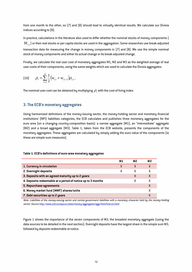
Using harmonised definitions of the money-issuing sector, the money-holding sector and monetary financial institutions’ (MFI) liabilities categories, the ECB calculates and publishes three monetary aggregates for the euro area (on a changing country-composition basis): a narrow aggregate (M1), an "intermediate" aggregate (M2) and a broad aggregate (M3). Table 1, taken from the ECB website, presents the components of the monetary aggregates. These aggregates are calculated by simply adding the euro value of the components (ie these are simple sum measures).

Table 1: ECB’s definitions of euro-area monetary aggregates

M1 M2 M3

1. Currency in circulation X X X 2. Overnight deposits X X X 3. Deposits with an agreed maturity up to 2 years X X 4. Deposits redeemable at a period of notice up to 3 months X X 5. Repurchase agreements X 6. Money market fund (MMF) shares/units X 7. Debt securities up to 2 years X

Note. Liabilities of the money-issuing sector and central government liabilities with a monetary character held by the money-holding sector. Source: http://www.ecb.europa.eu/stats/money/aggregates/aggr/html/hist.en.html

Figure 1 shows the importance of the seven components of M3, the broadest monetary aggregate (using the data sources to be detailed in the next section). Overnight deposits have the largest share in the simple sum M3, followed by deposits redeemable at notice.

12

Figure 1: Components of euro-area (changing composition) M3, seasonally adjusted, € trillions, September 1997 – February 2015

0

2

4

6

8

10

0

2

4

6

8

10

98 00 02 04 06 08 10 12 14

Currency in circulationOvernight depositsDeposits with an agreed maturity up to 2 yearsDeposits redeemable at a period of noticeRepurchase agreementsMoney market fund shares/unitsDebt securities up to 2 years

GR SICY,MT SK EE LV LT

Note: the vertical lines with the country-codes above indicate the dates when these countries joined the euro area. GR: Greece, SI: Slovenia, CY: Cyprus, MT: Malta, SK: Slovakia, EE: Estonia, LV: Latvia, LT: Lithuania.

4. Data sources and adjustments

Our aim is to calculate Divisia monetary aggregates corresponding to the three monetary aggregates published by the ECB, both for the changing composition euro area and for the first twelve member states that joined the euro (constant composition). We also aim to calculate the user cost of the three aggregates.

4.1 Data sources

Most of our data is from the ECB’s Statistical Data Warehouse. In addition,

• Data on currency issued was downloaded from the International Monetary Fund’s International Financial Statistics (IFS);

• Some German deposit rates were collected form the website of the Bundesbank;

• The return on debt securities up to two years is approximated by the Bank of America Merrill Lynch 1-3 Year Euro Financial Index.

Table 2 on the next page presents a summary of the data availability.

M3 M2

M1

13

Table 2: Summary of data availability (first available observation unless otherwise noted)

A: Monetary aggregates

Euro area (changing composition) Country-specific data

1. Currency in circulation SA: January 1980, NSA: September 1997 No, but currency issued is available from the IMF IFS

2. Overnight deposits SA: January 1980, NSA: September 1997 For a different reference sector*: September 1997, NSA, for the first 11 countries of the euro area; March 1998 for Greece; other seven members: from about two years before their euro entry

3. Deposits with an agreed maturity up to two years

September 1997, both NSA and SA same as for overnight deposits

4. Deposits redeemable at a period of notice

September 1997, both NSA and SA same as for overnight deposits

5. Repurchase agreements

September 1997, both NSA and SA Only for total repos** and for a different reference sector: same as for overnight deposits; for some countries there are only zero values

6. Money market funds September 1997, both NSA and SA same as for overnight deposits; for some countries there are only zero values

7. Debt securities up to two years

September 1997, both NSA and SA No***

Source: All data except currency issued by member states is from the ECB’s Statistical Data Warehouse.

Note: NSA: Neither seasonally nor working day adjusted; SA: Working day and seasonally adjusted.

* The reference sector used by the ECB for calculating the three monetary aggregates is “MFIs, central government and post office giro institutions”. Unfortunately, country-specific data is not available for this reference sector, but available for the reference sector “MFIs excluding ESCB”. ECSB = European System of Central Banks. The difference between the data for the two reference sectors of the euro-area aggregates is generally small or even zero, see Section 4.4 in which we plot the differences.

** The exact definition of repurchase agreements included in the ECB’s monetary aggregates is: “Repurchase agreements excluding repos with central counterparties”. Unfortunately, country-specific data is not available for this component, but only for total repurchase agreements, and for the reference sector described in * above. As we highlight in Section 4.4, central counterparties are excluded only from June 2010 onwards, causing a break in this component and also in M3.

*** Data on short term debt securities issued by MFIs is available, but it has a very different level and dynamics compared to the component included in M3.

14

B: Interest rates

Euro area (changing composition) Country-specific data

1. Currency in circulation assumed to be zero assumed to be zero 2. Overnight deposits January 2003 Harmonised data: January 2003 for the first 12

members; from the date of euro entry (or a few months earlier) for the newer members. Non-harmonised data*: December 1995-June/September 2003 for six countries (Austria, Finland, Greece, Italy, Netherlands and Spain); German data from Bundesbank for January 2000-December 2002

3. Deposits with an agreed maturity up to two years

January 2003 Harmonised data: same as for overnight deposits. Non-harmonised data*: December 1995-June/September 2003 for ten countries (first twelve euro members except Ireland and Luxembourg), but for somewhat different maturities

4. Deposits redeemable at a period of notice

January 2003 Harmonised data:January 2003 for five countries (Germany, Spain, Finland, France, Ireland); from later dates for 10 other countries, but there are many gaps in the data; in September 2014 data was available for 9 countries. Non-harmonised data*: December 1995-June/September 2003 for four countries (Belgium, Germany, Greece and Ireland)

5. Repurchase agreements

January 2003 Harmonised data: January 2003 for the four countries (Spain, France, Greece, Italy), but the Greek data end in 2011

6. Money market funds We use the Eonia rate; available from January 1995**

No

7. Debt securities up to two years

We use the Bank of America Merrill Lynch 1-3 Year Euro Financial Index; available from January 1996***

No

Source: All data except German overnight deposit rate in 2000-2002 and the Bank of America Merrill Lynch 1-3 Year Euro Financial Index are from the ECB’s Statistical Data Warehouse.

Note: * Some of the non-harmonised interest rate data must have very different definitions from the harmonised data and therefore cannot be used to proxy euro-area data for earlier years, as we discuss in the next section.

** Eonia, euro overnight index average, is a measure of the effective interest rate prevailing in the euro interbank overnight market. It is calculated as a weighted average of the interest rates on unsecured overnight lending transactions denominated in euro, as reported by a panel of contributing banks. See https://www.ecb.europa.eu/home/glossary/html/glosse.en.html#189

***The BofA Merrill Lynch Euro Financial Index tracks the performance of EUR denominated investment grade debt publicly issued by financial institutions in the eurobond or euro member domestic markets. The BofA Merrill Lynch 1-3 Year Euro Financial Index is a subset of The BofA Merrill Lynch Euro Financial Index including all securities with a remaining term to final maturity less than 3 years. Qualifying securities must have at least one year remaining term to final maturity, at least 18 months to final maturity at point of issuance, a fixed coupon schedule and a minimum amount outstanding of EUR 250 million See: http://www.mlindex.ml.com/gispublic/bin/getdoc.asp?fn=EB01&source=indexrules

In order to check the consistency of the money components with the simple sum aggregates M1, M2 and M3 published by the ECB, we calculated the sum of the components: the sums calculated by us were identical to the monetary aggregates published by the ECB, both for the unadjusted and the seasonally adjusted data.

15

In addition to monetary aggregates, the ECB publishes data on monthly transactions and the percent changes in a co-called index of notional stocks.

Transactions data are derived by adjusting the change in stocks with reclassification, revaluation and exchange rate adjustment of the components. Such changes and breaks in the series should be disregarded when growth rates of money stocks are calculated or when a time series is used for econometric analysis.

The index of notional stocks is calculated as a chain-index, by multiplying the previous period value of notional stock with the percent increased derived from transaction data, where the percent change is calculated by dividing the transaction in a given month with the outstanding amounts of the asset at the end of the period. See equation 4.3.1 and sections 4.2 and 4.3 of ECB (2012a) for details.

4.2 Approximating non-available euro-area average interest rates for 2001-2002

Panel B of Table 2 shows that interest rates for four components of M3 are available for the euro area (changing composition) starting in January 2003. We approximate these four interest rate series for 2001-2002 using country-specific data and explain the data limitations that do not allow a proper approximation of two of these four interest rate series pre-2000 with a sufficient coverage. Approximating for 2000 would be possible, but we decided to start our sample in January 2001 because Greece joined the euro area in this month and our focus is on a constant composition euro-area aggregate for the first twelve members. Starting our sample period in January 2001 implied that no aggregation is needed for countries with different currencies. Also, in 2000 Greek interest rates behave very differently from those of euro-area members that joined in 1999, which would make it more difficult to interpret their aggregate in 2000.

Overnight deposit rate

The ECB publishes country-specific interest rates on overnight deposits starting in January 2003 for all the euro-area countries at that time (data for newer euro-area members is available from later dates). The series are regularly updated (the latest data is for February 2015). For seven of the first twelve members, separate series are available from the ECB for December 1995 – June or September 2003. We could find pre-2003 data only at the Bundesbank website for Germany, but not at the central bank websites of the other larger euro-area countries.

The first seven panels of Figure 2 plot the new and the old ECB series for the seven countries for which the ECB publishes pre-2003 data, along with the euro-area average overnight deposit rate and the 1-week EURIBOR. For Finland, Italy and Greece the old and new data match quite well. For Austria and the Netherlands the old series are very different from the new series and the old series are almost constant at a time when all other interest rate series (of these two countries and of other euro-area countries) exhibited an increasing trend in late 1999 and then a falling trend in mid-2001. Because of these discrepancies, we do not use the pre-2003 Austrian and Dutch time series. The old Spanish series are also different in levels from the new Spanish series, but its dynamics are quite plausible given the dynamics in other countries. Therefore, for Finland, Italy, Greece and Spain we make use of the old ECB series and chain them backwards to the new ECB series, by adding to the old series the average spread between the new and the old series in the period when both are available (ie in the first seven or nine months of 2003; see the thick green lines on the charts).

For Germany, the Bundesbank publishes effective overnight interest rates separately for German households and non-financial corporations, for two sample periods: a ‘new’ one starting in January 2003, which is regularly updated, while the ‘old’ one is available for January 2000 – December 2002. We used the volume of

16

households’ and non-financial corporations’ overnight deposit outstanding quantities (available from January 2003) to calculate the average overnight deposit rate. The weighted average overnight deposit rate of the ‘new’ series calculated by us was identical to the German overnight deposit rate published by the ECB in each month during January 2003-February 2015. Lacking pre-2003 quantities on deposits, we used the January 2003 volume of deposits to weight the interest rates for the two sectors pre-2003. Since the shares of households and nonfinancial corporations in overnight deposits were relatively stable after 2003, using the January 2003 values for calculating a weighted average for 2000-2002 likely does not introduce any major distortion. As the last panel of Figure 2 shows, the old and new series are nicely connected and therefore we use the old series for 2000-2002.

Figure 2: Overnight deposit rates for seven euro-area countries with available data before 2003, January 1995 – February 2015

-1

0

1

2

3

4

5

-1

0

1

2

3

4

5

96 98 00 02 04 06 08 10 12 14

Austria: Old ECB dataAustria: New ECB dataAustria: difference between old and new ECB dataEuro area: ECB dataEuro area: 1 week EURIBOR

Austria

-1

0

1

2

3

4

5

-1

0

1

2

3

4

5

96 98 00 02 04 06 08 10 12 14

Finland: Old ECB dataFinland: New ECB dataFinland: difference between old and new ECB dataEuro area: ECB dataEuro area: 1 week EURIBOR

Finland

-1

0

1

2

3

4

5

6

7

-1

0

1

2

3

4

5

6

7

96 98 00 02 04 06 08 10 12 14

Greece: Old ECB dataGreece: New ECB dataGreece: difference between old and new ECB dataEuro area: ECB dataEuro area: 1 week EURIBOR

Greece

-1

0

1

2

3

4

5

6

-1

0

1

2

3

4

5

6

96 98 00 02 04 06 08 10 12 14

Italy: Old ECB dataItaly: New ECB dataItaly: difference between old and new ECB dataEuro area: ECB dataEuro area: 1 week EURIBOR

Italy

-1

0

1

2

3

4

5

-1

0

1

2

3

4

5

96 98 00 02 04 06 08 10 12 14

Netherlands: Old ECB dataNetherlands: New ECB dataNetherlands: difference between old and new ECB dataEuro area: ECB dataEuro area: 1 week EURIBOR

Netherlands

-1

0

1

2

3

4

5

-1

0

1

2

3

4

5

96 98 00 02 04 06 08 10 12 14

Spain: Old ECB dataSpain: New ECB dataSpain: difference between old and new ECB dataEuro area: ECB dataEuro area: 1 week EURIBOR

Spain

-1

0

1

2

3

4

5

-1

0

1

2

3

4

5

96 98 00 02 04 06 08 10 12 14

Germany: Old Bundesbank dataGermany: New Bundesbank dataEuro area: ECB dataEuro area: 1-week EURIBOR

Germany

After these amendments, we have pre-2003 data on overnight deposits for five countries: Germany (from January 2000) and Finland, Italy, Greece and Spain (from December 1995). The group of the latter four countries is far from being sufficient to approximate a euro-area average before 2000. Greece, which joined the euro area in January 2001, exhibited very different interest rate developments relative to the other euro-area countries before joining the euro, and therefore mixing Greek data with the data of the other eleven members

17

before Greece’s entry to the euro area might lead to an aggregate that is difficult to interpret. We therefore approximate the missing data for the euro-area average for only 2001-2002.

While the five countries together account for about half of the euro area, calculating a weighted average of the data of the five countries (eg using weights from their shares in monetary aggregates) would be appropriate only if they are representative of the average. However, as Figure 2 shows, Germany, the euro area’s largest country, used to have persistently higher overnight deposit rates than the euro-area average, while Finland and Spain used to have lower rates. Italian and Greek rates were the closest to the euro-area average. The 2005 drop in the euro-area average is mostly visible in Spain (see the right panel of Figure 4). Figure 3 shows that there was a non-constant and sizeable spread between the average of these five countries and the euro-area average.

Figure 3: Overnight deposit rates: euro area versus the average of the five countries, January 2003 – February 2015

0.0

0.4

0.8

1.2

1.6

2.0

0.0

0.4

0.8

1.2

1.6

2.0

2004 2006 2008 2010 2012 2014

Euro-area (changing composition)Five euro-area countries

Note: the five countries are Finland, Germany, Greece, Italy and Spain. We weighted the deposit rates of these five countries with the shares of these countries in the aggregate outstanding volume of overnight deposit of the five countries.

We therefore decided not to weight the country-specific rates of the five countries using their shares in aggregate volume of the five countries, but we estimated a regression to determine the weights. Specifically, we regressed the euro-area average rate on the interest rates of the five countries as explanatory variables in the period 2003-2006 (a period that may have similarities to the 2001-2002 period for which we aim to approximate the euro-area average). We do not include an intercept in the regression and constrain the parameters to sum up to one.

Table 3 shows the regression results. Italy has the largest estimated weight (32 percent), perhaps because Italian interest rates were the most similar to the interest rates of those euro-area countries which are omitted from the regression due to missing data. The left panel of Figure 4 shows the fitted values for 2003-2006 and the predicted values for 2001-2002. The right panel of Figure 4 compares the euro-area average to the data of the five counties.

18

Table 3: OLS regression of euro-area overnight deposit rate on the overnight deposit rates of five countries

Coefficient Std. Error t-StatisticGermany 0.216 0.016 13.4Finland 0.153 0.021 7.3Italy 0.321 0.026 12.2Spain 0.190 0.017 10.9Greece 0.121

Note: estimated regression: ( ) ttGRtEStITtFItDEtEA urrrrrr +−−−−++++= ,14321,4,3,2,1, 1 βββββββββ. Since the parameter of the Greek interest rate is constrained, its standard error is not estimated. The sample period includes monthly data between January 2003 and December 2006. The coefficient of determination (R2) is 0.993.

Figure 4: Overnight deposit rates for the euro area and its approximation for 2001-2002, January 2001 – February 2015

0.0

0.4

0.8

1.2

1.6

2.0

0.0

0.4

0.8

1.2

1.6

2.0

2002 2004 2006 2008 2010 2012 2014

Euro-area overnight deposit rate (ECB data)Regression fit for 2003-06 and estimate for 2001-2002

Predictionperiod

Estimation period

0.0

0.4

0.8

1.2

1.6

2.0

0.0

0.4

0.8

1.2

1.6

2.0

2002 2004 2006 2008 2010 2012 2014

Euro area Finland GermanyGreece Italy Spain

Deposits with an agreed maturity up to 2 years

Similarly to other deposit rates, the ECB publishes euro-area average (changing composition) and country-specific interest rates from January 2003 on deposits with an agreed maturity of up to 2 years. For the following ten countries, the ECB publishes separate times series from December 1995 to either June or September 2003:

• Deposits with agreed maturity, up to 1 year: Austria, Belgium, Germany, Greece and Portugal;

• Deposits with agreed maturity, over 1 and up to 2 years: France, Italy, the Netherlands and Spain;

• Deposits with agreed maturity, total: Finland.

Presumably, deposit rates for these maturities should not differ much from the rates on deposits with maturity up to 2 years.

19

Figure 5 on the next page shows that the difference between the old and the new series are indeed typically small with perhaps the exception of Belgium. Yet for Belgium the dynamics of the old and new series are very similar in the period when both rates are available. Therefore, we chain the old series to the new series similarly as we did with the overnight deposit rates, ie by adding to the old series the average spread between the new and old series in 2003.

Figure 5 also shows that the differences compared to the euro-area average interest rate (which is available from 2003) are typically smaller (at least up to the crisis) than in the cases of overnight deposits rates. For example, the German term deposit rate was practically identical to the euro-area average in 2003-08, while Figure 2 showed that the overnight German deposit rate was higher than the euro-area average. Also, Figure 2 reports that Greek interest rates developed very differently from the rates in other euro-area countries before Greece joined the monetary union in 2001.

20

Figure 5: Rates on deposits with an agreed maturity up to 2 years* for ten euro-area countries with available data before 2003, January 1995 – February 2015

0

1

2

3

4

5

6

0

1

2

3

4

5

6

96 98 00 02 04 06 08 10 12 14

Austria: Old ECB dataAustria: New ECB dataAustria: difference between old and new ECB dataEuro area: ECB dataEuro area: 12-month EURIBOR

Austria

0

1

2

3

4

5

6

0

1

2

3

4

5

6

96 98 00 02 04 06 08 10 12 14

Belgium: Old ECB dataBelgium: New ECB dataBelgium: difference between old and new ECB dataEuro area: ECB dataEuro area: 12-month EURIBOR

Belgium

-1

0

1

2

3

4

5

6

-1

0

1

2

3

4

5

6

96 98 00 02 04 06 08 10 12 14

Finland: Old ECB dataFinland: New ECB dataFinland: difference between old and new ECB dataEuro area: ECB dataEuro area: 12-month EURIBOR

Finland

0

1

2

3

4

5

6

0

1

2

3

4

5

6

96 98 00 02 04 06 08 10 12 14

France: Old ECB dataFrance: New ECB dataFrance: difference between old and new ECB dataEuro area: ECB dataEuro area: 12-month EURIBOR

France

0

1

2

3

4

5

6

0

1

2

3

4

5

6

96 98 00 02 04 06 08 10 12 14

Germany: Old ECB dataGermany: New ECB dataGermany: difference between old and new ECB dataEuro area: ECB dataEuro area: 12-month EURIBOR

Germany

0

2

4

6

8

10

12

14

16

0

2

4

6

8

10

12

14

16

96 98 00 02 04 06 08 10 12 14

Greece: Old ECB dataGreece: New ECB dataGreece: difference between old and new ECB dataEuro area: ECB dataEuro area: 12-month EURIBOR

Greece

0

2

4

6

8

10

0

2

4

6

8

10

96 98 00 02 04 06 08 10 12 14

Italy: Old ECB dataItaly: New ECB dataItaly: difference between old and new ECB dataEuro area: ECB dataEuro area: 12-month EURIBOR

Italy

-1

0

1

2

3

4

5

6

-1

0

1

2

3

4

5

6

96 98 00 02 04 06 08 10 12 14

Netherlands: Old ECB dataNetherlands: New ECB dataNetherlands: difference between old and new ECB dataEuro area: ECB dataEuro area: 12-month EURIBOR

Netherlands

0

1

2

3

4

5

6

7

8

0

1

2

3

4

5

6

7

8

96 98 00 02 04 06 08 10 12 14

Spain: Old ECB dataSpain: New ECB dataSpain: difference between old and new ECB dataEuro area: ECB dataEuro area: 12-month EURIBOR

Spain

0

1

2

3

4

5

6

7

8

9

0

1

2

3

4

5

6

7

8

9

96 98 00 02 04 06 08 10 12 14

Portugal : Old ECB dataPortugal : New ECB dataPortugal: difference between old and new ECB dataEuro area: ECB dataEuro area: 12-month EURIBOR

Portugal

* The new country-specific data (available from January 2003 onwards) and the euro-area average (also available from January 2003 onwards) refer to deposits with an agreed maturity up to 2 years. The old series available for December 1995-June/September 2003 refer to deposits with different maturities: up to 1 year (Austria, Belgium, Germany, Greece and Portugal), over 1 and up to 2 years (France, Italy, the Netherlands and Spain) and total (Finland).

21

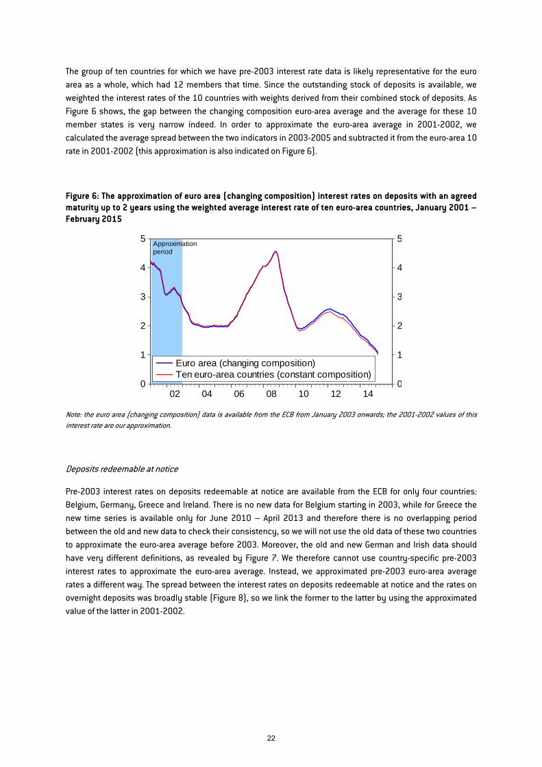
The group of ten countries for which we have pre-2003 interest rate data is likely representative for the euro area as a whole, which had 12 members that time. Since the outstanding stock of deposits is available, we weighted the interest rates of the 10 countries with weights derived from their combined stock of deposits. As Figure 6 shows, the gap between the changing composition euro-area average and the average for these 10 member states is very narrow indeed. In order to approximate the euro-area average in 2001-2002, we calculated the average spread between the two indicators in 2003-2005 and subtracted it from the euro-area 10 rate in 2001-2002 (this approximation is also indicated on Figure 6).

Figure 6: The approximation of euro area (changing composition) interest rates on deposits with an agreed maturity up to 2 years using the weighted average interest rate of ten euro-area countries, January 2001 – February 2015

0

1

2

3

4

5

0

1

2

3

4

5

02 04 06 08 10 12 14

Euro area (changing composition)Ten euro-area countries (constant composition)

Approximationperiod

Note: the euro area (changing composition) data is available from the ECB from January 2003 onwards; the 2001-2002 values of this interest rate are our approximation.

Deposits redeemable at notice

Pre-2003 interest rates on deposits redeemable at notice are available from the ECB for only four countries: Belgium, Germany, Greece and Ireland. There is no new data for Belgium starting in 2003, while for Greece the new time series is available only for June 2010 – April 2013 and therefore there is no overlapping period between the old and new data to check their consistency, so we will not use the old data of these two countries to approximate the euro-area average before 2003. Moreover, the old and new German and Irish data should have very different definitions, as revealed by Figure 7. We therefore cannot use country-specific pre-2003 interest rates to approximate the euro-area average. Instead, we approximated pre-2003 euro-area average rates a different way. The spread between the interest rates on deposits redeemable at notice and the rates on overnight deposits was broadly stable (Figure 8), so we link the former to the latter by using the approximated value of the latter in 2001-2002.

22

Figure 7: Interest rates on deposits redeemable at notice for the two euro-area countries with available data both before and after 2003, January 1995 – February 2015

-1

0

1

2

3

4

5

6

-1

0

1

2

3

4

5

6

96 98 00 02 04 06 08 10 12 14

Germany: Old ECB dataGermany: New ECB dataGermany: difference between old and new ECB dataEuro area: ECB dataEuro area: 12-month EURIBOR

Germany

0

1

2

3

4

5

6

0

1

2

3

4

5

6

96 98 00 02 04 06 08 10 12 14

Ireland: Old ECB dataIreland: New ECB dataIreland: difference between old and new ECB dataEuro area: ECB dataEuro area: 12-month EURIBOR

Ireland

Figure 8: The spread between euro-area average interest rates on deposits redeemable at notice and overnight deposit rate, January 2001 – February 2015

0.0

0.5

1.0

1.5

2.0

2.5

3.0

3.5

0.0

0.5

1.0

1.5

2.0

2.5

3.0

3.5

02 04 06 08 10 12 14

Euro area: Interest rate on deposits redeemable at noticeEuro area: Interest rate on overnight depositsSpread between the two

Constantspreadassumption

Repurchase agreements

Pre-2003 data on repurchase agreements is available only for Spain, which is not sufficient to approximate the euro-area average. We approximate the euro-area repo rate for 2001-2002 by observing that the spread between the repo rate and the EURIBOR was rather stable in 2003-2005 (Figure 9). We therefore subtract 10 basis points (the average difference between the 1-month EURIBOR and the repo rate in 2003-2005) from the 1-month EURIBOR to approximate the pre-2003 average euro-area repo rate.

23

Figure 9: Interest rates on repurchase agreements and the EURIBOR, January 2001 – February 2015

0

1

2

3

4

5

0

1

2

3

4

5

2000 2002 2004 2006 2008 2010 2012 2014

Euro area: Interest rate on repurchase agreementsEuro area: 1-week EURIBOREuro area: 1-month EURIBOREuro area: 3-month EURIBOR

4.3 The benchmark rate

The so-called benchmark rate is the rate of return on an asset that does not provide monetary service, only investment income. As Barnett (1978, 1980) proved, the benchmark rate is needed to derive the weights of the components for the Divisia monetary indices and to calculate the user cost of money.

Such a benchmark asset is hardly observable and therefore researchers/institutions adopted different approaches to approximate the benchmark rate. The most widely used assumption is to add a spread to the maximum return of some observed assets. The selection of the maximum return (at each point in time) is called the ‘upper envelope’ approach and in most cases the components of the money stock are considered. The spread which is added to the maximum return to get the benchmark rate is called the ‘liquidity services premium’.

For example, Stracca (2004) proxies the benchmark rate by adding 60 basis points to the rate on marketable instruments (that he defined as the sum of three components that differentiate ECB’s M2 and M3: repurchase agreements, money market funds and debt securities up to 2 years). Jones and Stracca (2012) adopted the same approach. El-Shagi and Kelly (2013) adopted two proxies: (1) adding 100 basis points to the return on the maximum return of the components of the money stock, (2) adding a variable premium to the maximum return of the components amounting to the spread between the ten-year and one-year government bond yields. Up to 2005, the Bank of England proxied the benchmark rate as the interest rate on three-month Local Government (LG) bills plus a 200 basis point spread, but then switched to an envelope approach, whereby the benchmark asset is the M4 component that pays the highest interest rate (see Hancock, 2005). The Center for Financial Stability (CFS) uses an envelope approach applied to all components of the money stock plus a loan rate8 from 1997, the date from when this loan rate is available. For earlier years, 100 basis points are added to the yield on the highest yielding asset of M4 (see Barnett et al, 2013).

We find the fixed-spread assumption to be ad hoc and therefore we sought an alternative. Since only bank debt up to 2 years maturity is included in euro-area M3, we also considered the yield on bank debt for longer

8 The loan rate considered is the “Weighted average effective loan rate, low risk, 31 to 365 days, all commercial banks”. The reason for the use of this rate is that it acts as an upper limit to the interest rate a bank will offer on any deposit category, because a bank will not pay out to its depositors more than it earns in interest on the short-term loans it makes.

24

maturities. BofA Merrill Lynch Year Euro Bond Indices are also calculated for maturities 3-5 years, 5-7 years, 5-10 years and over 10 years. Bank debt with such a long maturity may have characteristics similar to the theoretical benchmark asset. Longer maturity bank debt had higher returns than the returns on the components of M3. The left panel of Figure 10 plots the benchmark rate and the own rate of seven money components. The right panel of Figure 10 shows the difference between the benchmark rate and the maximum rate among the M3 components. This spread, which can be regarded as an estimate of the liquidity services premium, was quite variable both before and after the outbreak of the global financial and economic crisis.

Figure 10: The benchmark rate, rates on the components of M3 and the liquidity premium (percent per year), January 2001 – February 2015

0

2

4

6

8

10

0

2

4

6

8

10

2002 2004 2006 2008 2010 2012 2014

Overnight depositsDeposits up to 2 yearsDeposits redeemable with noticeRepurchasement agreementsMoney market fundsDebt securities up to two yearsBenchmark rate

Rates of return on M3 componentsand the benchmark rate

0.0

0.5

1.0

1.5

2.0

2.5

0.0

0.5

1.0

1.5

2.0

2.5

2002 2004 2006 2008 2010 2012 2014

Benchmark rate minus max rate of money components

Liquidity services premium

Note: The own rate on currency is zero and is not shown on the left panel. The benchmark rate is the maximum of the rate on bank debt with the following maturities: 5-7 years, 5-10 years and over 10 years.

A drawback of our selection of the benchmark asset is that it should be risk-free in principle, while the longer-maturity bank debts we consider are not risk free. However, most components of the money stock involve risk, including the 2-year maturity bank debt and bank deposits9. The rate on any risk-free benchmark asset would likely be lower than the return on many components of the monetary aggregates. For example, the return on 10-year German government bonds, which is probably a safe asset, is only 0.8 percent per year at the time of writing this paper, which is below all but two interest rates indicated on the left panel of Figure 10. While Barnett, Liu and Jensen (1997) developed an aggregation formula for the case of risk by using the consumption capital asset pricing model (CCAPM), that model is not without problems and the available Divisia monetary aggregates for the EU and US are also not risk-adjusted. We therefore do not adjust our aggregation method to risk but leave this issue for further research.

9 Note that in Denmark (a non-euro area EU country) and in Cyprus (a euro-area country) depositors having deposits over the €100,000 guaranteed amount suffered losses during the restructuring of some banks. Moreover, deposits were withdrawn to a significant level from several euro-area periphery countries and transferred to other (safer) euro-area countries. This suggests that even in the cases when depositors did not suffer any actual loss, many of them regarded their deposits as unsafe in euro-area periphery countries.

25

4.4 Approximating constant country composition monetary aggregates

The ECB indicators of euro-area outstanding monetary aggregates (M1, M2, M3) and their components (see Table 1) are subject to two major shortcomings:

• First, they relate to the changing country-composition euro-area and hence there was a level shift in these indicators whenever a new member joined the euro area.

• Second, they are subject to reclassification changes, such as halving the outstanding stock of the measure of repurchase agreements included in the ECB’s M3 aggregate in June 2010 (see the penultimate panel of Figure 11, which shows that central counterparties were excluded from repurchase agreements only from June 2010 onwards10).

For economic analysis, such level shifts should be eliminated. When each new country joins the euro area, the outstanding stock of money increases because of the inclusion of this new member, but this is not an increase in the money stock. The use of aggregates which do not include a level shift at the time of enlargement is therefore preferable. Moreover, the positions of monetary and financial institutions (MFIs) in the original euro-area countries (like Germany, etc.) are also reclassified after the entry of a new country into the euro area, because the new member belongs to the euro area from the date of entry, while prior to entry it was classified as part of the rest of the world.

Beyond data on outstanding money stocks and their components, the ECB publishes data on transactions for the changing-composition euro area (but not for individual countries). The ECB’s transactions data treat enlargement as a special case of reclassification (see Section 4.3.2 of ECB (2012a)). Therefore, if monetary aggregates are calculated as cumulative transactions, there is no sudden jump in the monetary aggregates at the time of enlargement. However, after enlargement, transactions data include the new member states as well and therefore the country-composition of transactions data is changing with enlargement, which is a drawback. A further plus of the use of transactions data is that all other kinds of reclassification problems are eliminated, like the problem with the repurchase transaction mentioned above.

The countries that joined the euro area after 2001 (Slovenia, Cyprus, Malta, Slovakia, Estonia, Latvia and Lithuania) are relatively small and therefore the impact of the composition change should be small too11. Nevertheless, we calculated aggregates which do not suffer from enlargement-related and other level shifts. We create four versions of both the Divisia index and simple-sum measures:

1. EA: Changing-composition euro-area aggregates using data on outstanding stocks.

o Advantage: consistent with the outstanding M1, M2 and M3 simple-sum aggregates published by the ECB.

o Disadvantage: These aggregates suffer from both drawbacks mention at the beginning of this section: level shifts due to both euro-area enlargement and other reclassification changes.

10 See Box 3 on page 28 of ECB (2012b) for the motivation of this exclusion. 11 Note that Greece joined the euro area in 2001 and we calculate our euro-area aggregates starting in 2001 and therefore Greece’s entry does not lead to a compositional change in our aggregates.

26

2. EA12: Constant-composition euro-area aggregates for the first twelve members of the euro area using data on outstanding stocks12.

o Advantage: enlargement-related level shifts are excluded.

o Disadvantage: other reclassifications lead to level shifts; the country-specific data of the new members which were subtracted from the changing-composition euro-area aggregates refer to different sector.

Five of the seven components of M3

For the five components of M3 indicated in Figure 11, we calculated the constant-composition euro-area 12 aggregate by subtracting from the total (changing-composition) euro-area values the values of the seven new members starting from the date of their euro-area membership (i.e. we subtract the green line from the blue line of Figure 11).

This calculation is not perfect, because country-specific data is not available for the reference sector which is considered for M1, M2 and M3 by the ECB. As already documented in the notes to Panel A of Table 2, euro-area aggregate data on the components of the ECB’s monetary aggregates considers the sector “MFIs, central government and post office giro institutions”. Unfortunately, country-specific data is not available for this reference sector, but for the sector “MFIs excluding ESCB”. For the repos “Repurchase agreements excluding repos with central counterparties” is included in the ECB’s M3 indicator, but country-specific data is available only for total repos. Such differences may limit the accuracy of our constant country composition calculations, but fortunately the difference between the data referring to the two reference sectors of the euro-area aggregates is generally small, except for repos from June 2010 onwards (Figure 11). For repos, Figure 11 suggests that data on central counterparties was excluded only from June 2010 onwards and therefore there is a break in the series which is included in the ECB’s M3 aggregate, and consequently there is a break in the M3 aggregate too.

Currency in circulation

It is not possible to obtain country-specific data on currency in circulation, because cash flows freely within the monetary union. Yet using data on currency issued, we approximate the euro-area 12 by combining IMF and ECB data to proxy country-specific values. The IMF International Financial Statistics (IFS) publishes data on “Currency issued” for 16 of the 19 euro-area members (not available for Slovakia, Latvia and Lithuania in the December 2014 version of the IFS), plus for the euro area13.

The left and middle panels of Figure 12 show that there is a consistency problem with the IMF data: in 2001-2006, the sum of the values of the first twelve members of the euro area should be equal to the euro-area aggregate, but this equality holds only in 2001. In 2002-2005 there is a sizeable gap. On the other hand, the middle panel also shows that from 2003 onwards, the share of the first twelve members in the overall euro-area aggregate was stable for periods when no new member joined and declined only when a new member joined. This observation suggests that the 2001-

12 Missing data does not allow the estimation of constant-composition aggregates for the current 19 members of the euro area. 13 The idea to use IMF data on currency issued originated in the work of El-Shagi and Kelly (2013), who calculated Divisia money indicators for six euro-area countries, though they did not combine the IMF data on currency issued and the ECB data on currency in circulation.

27

2002 data may be incorrect, but data from 2003 onwards may be correct apart from perhaps a level problem.

The right panel of Figure 12 shows that the data on currency issued is higher by about 5-10 percent than the data on currency is circulation in most years, which is sensible. This panel also reveals that in 2002 there seems to be an unusually large difference between the two indicators, suggesting that there may be a data issue in 2002.

Our aim is to estimate and separate out the volume of currency in circulation in the seven newer euro-area members that joined between 2007-2015. To this end, we calculate the ratio of currency issued in Slovenia over the total currency issued in the euro area in each month of 2007-2014 (both are IMF data) and use this share to multiply the euro-area aggregate currency in circulation data of the ECB to get an estimate of the currency in circulation in Slovenia. We calculate the same (time-varying monthly) ratio for Cyprus, Malta and Estonia starting from the dates when they became members of the euro area. Lacking IMF data on Slovakia, Latvia and Lithuania, we cannot do the same exercise for these two countries. However, as the middle panel of Figure 12 reveals, the share of the first twelve members in total euro area declined at the time when Slovakia and Latvia joined, and using the magnitude of this decline, we can calculate the shares of these three countries too in total (changing composition) euro-area aggregate currency issued. Lithuania joined the euro area recently in January 2015 and we do not have yet IMF data for January 2015. For the time being we approximate currency in circulation in Lithuania by assuming that the ratio of cash to overnight deposits is the same in Lithuania and in Latvia. When data will be available for Lithuania, we will adopt the same calculation method we used for Latvia.

Bank debt up to two years maturity

The ECB does not provide a country-specific breakdown of the 7th component of M3, bank debt up to two years maturity, while other data, such as short-term securities other than shares of banks (for which country-specific data is available) is not suitable14. Given that the share of the seven newer members in the higher numbered components of M3 is minuscule (Table 4) and their share in bank debt could be similar, and that bank debt is a small component in M3 (Figure 1), we use the total (changing composition) bank debt component of M3 in our constant-composition aggregates.

We first calculated the seasonally non-adjusted aggregates for the euro-area 12 group and then adjusted the resulting series seasonally.

3. EAN: Euro area (changing composition) "notional outstanding stock" calculated by cumulating data on transactions.

o Advantage: sudden breaks in the series are eliminated, including level shifts related to euro area enlargement.

o Disadvantage: transactions data refer to the changing composition euro area and so while there is no level shift in the indicator at the time of enlargement, starting from the date

14 The ECB publishes country-specific data on short-term securities other than shares of monetary financial institutions (MFIs), which may be a reasonable proxy for bank debt up to two years. However, the bank debt indicator used as a component of M3 was 72 percent in September 1997 and only 14 percent in July 2014 of the aggregate of the country-specific data on short-term securities other than shares of MFIs, suggesting that both the level and the dynamics of these two variables are very different.

28

enlargement, transitions in the new member are included, leading to time-variation in country composition.

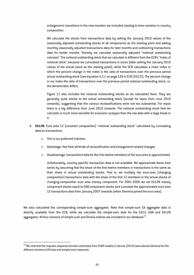
We calculate the stocks from transactions data by setting the January 2010 values of the seasonally adjusted outstanding stocks of all components as the starting point and adding monthly seasonally adjusted transactions data for later months and subtracting transactions data for earlier months. Thereby we calculate seasonally adjusted “notional outstanding volumes”. The notional outstanding stock that we calculate is different from the ECB's "Index of notional stock", because we cumulated transactions in euros (after setting the January 2010 values of the actual stock as the starting point), while the ECB calculates a chain index in which the percent change in the index is the ratio of transactions over the previous period actual outstanding stock (see equation 4.3.1 on page 126 in ECB (2012)). The percent change in our index the ratio of transactions over the previous period notional outstanding stock, i.e. the denominator differs.

Figure 11 also includes the notional outstanding stocks as we calculated them. They are generally quite similar to the actual outstanding stock (except for repos from June 2010 onwards), suggesting that the various reclassifications were not too substantial. For repos there is a big difference from June 2010 onwards. The notional outstanding stock that we calculate is much more sensible for economic analysis than the raw data with a large break in it.

4. EA12N: Euro area 12 (constant composition) "notional outstanding stock" calculated by cumulating data on transactions.

o This is our preferred indicator.

o Advantage: free from all kinds of reclassification and enlargement-related changes.

o Disadvantage: transactions data for the first twelve members of the euro area is approximated.

Unfortunately, country-specific transaction data is not available. We approximate these time series by assuming that the share of the first twelve members in transactions is the same as their share in actual outstanding stocks. That is, we multiply the euro-area (changing composition) transactions data with the share of the first 12 members in the actual stocks of changing-composition euro area money component. For 2001-2006 we set EA12N money component stocks equal to EAN component stocks and cumulate the approximated euro-area 12 transactions data from January 2007 onwards (when Slovenia joined the euro area).

We also calculated the corresponding simple-sum aggregates. Note that simple-sum EA aggregate data is directly available from the ECB, while we calculate the simple-sum data for the EA12, EAN and EA12N aggregates. All four versions of simple-sum and Divisia-indices are included in our database15.

15 We note that the impulse-response function estimates from SVAR models in Darvas (2014) were almost identical for the different versions of Divisia and simple-sum measures.

29

Figure 11: Comparison of euro area (changing composition) data regarding two reference sectors, the combined contribution of seven newer members to euro area data, and our notional outstanding stock indicators, in euros, September 1997 – February 2015

0

1,000

2,000

3,000

4,000

5,000

0

1,000

2,000

3,000

4,000

5,000

98 00 02 04 06 08 10 12 14

Overnight deposits

0

500

1,000

1,500

2,000

2,500

0

500

1,000

1,500

2,000

2,500

98 00 02 04 06 08 10 12 14

Deposits up to 2 years

0

400

800

1,200

1,600

2,000

2,400

0

400

800

1,200

1,600

2,000

2,400

98 00 02 04 06 08 10 12 14

Deposits redeemable at notice

0

100

200

300

400

500

600

0

100

200

300

400

500

600

98 00 02 04 06 08 10 12 14

Repurchase agreements

0100200300400500600700800900

0100200300400500600700800900

98 00 02 04 06 08 10 12 14

Euro area, Reference sector: MFIs, central government and post office giro institutionsEuro area, Reference sector: MFIs excluding ESCBContribution of seven newer members to euro area aggregateEuro area: calculated by cumulating transactions

Money market funds

Note: the components indicated by blue lines are included in the ECB’s monetary aggregates, while country-specific data is available for the aggregates corresponding to the red lines. The green lines, showing the aggregate data of seven newer members, relate to the reference sector “MFIs excluding ECSB” and each of these newer members are included from the date of their euro entry onwards. ECSB = European System of Central Banks. The purple line indicates the “notional outstanding stock” as calculated by us, ie the indicator we denoted EAN. The notional outstanding stock is seasonally adjusted, but the other three lines are not. For repurchase agreements, the blue line indicates “Repos excluding central counterparties”, while the red line indicates “Total repos”: comparison of the two lines underlines that central counterparties were excluded only from June 2010 onwards.

30

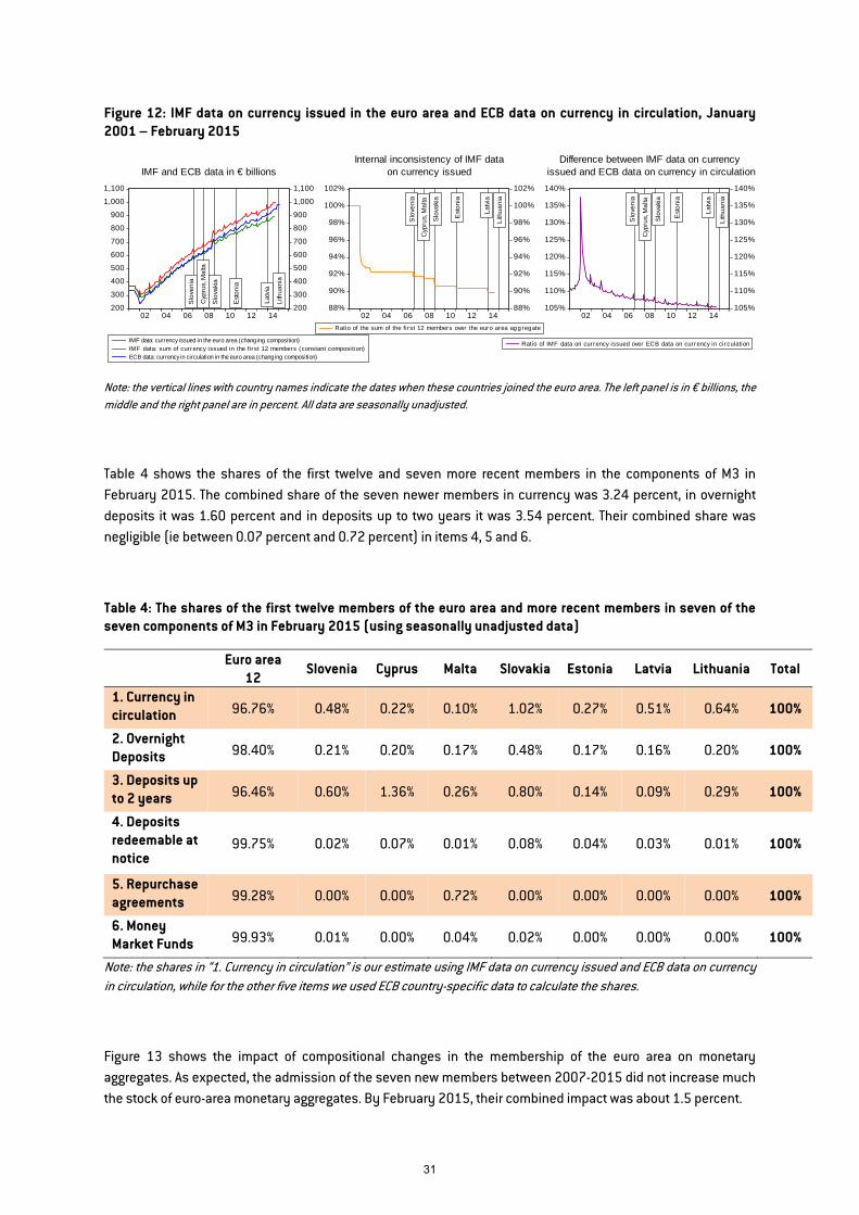
Figure 12: IMF data on currency issued in the euro area and ECB data on currency in circulation, January 2001 – February 2015

200

300

400

500

600

700

800

900

1,000

1,100

200

300

400

500

600

700

800

900

1,000

1,100

02 04 06 08 10 12 14

IMF data: currency issued in the euro area (changing composition)IMF data: sum of currency issued in the first 12 members (constant composition)ECB data: currency in circulation in the euro area (changing composition)

IMF and ECB data in € billions

Slo

ven

ia

Cyp

rus,

Ma

lta

Slo

vaki

a

Est

on

ia

La

tvia

Lith

ua

nia

88%

90%

92%

94%

96%

98%

100%

102%

88%

90%

92%

94%

96%

98%

100%

102%

02 04 06 08 10 12 14

Ratio of the sum of the first 12 members over the euro area agg regate

Internal inconsistency of IMF dataon currency issued

Slo

ven

ia

Cyp

rus,

Ma

lta

Slo

vaki

a

Est

on

ia

La

tvia

Lith

ua

nia

105%

110%

115%

120%

125%

130%

135%

140%

105%

110%

115%

120%

125%

130%

135%

140%

02 04 06 08 10 12 14

Ratio of IMF data on currency issued over ECB data on currency in circulation

Difference between IMF data on currency issued and ECB data on currency in circulation

Slo

ven

ia

Cyp

rus,

Ma

lta

Slo

vaki

a

Est

on

ia

La

tvia

Lith

ua

nia

Note: the vertical lines with country names indicate the dates when these countries joined the euro area. The left panel is in € billions, the middle and the right panel are in percent. All data are seasonally unadjusted.

Table 4 shows the shares of the first twelve and seven more recent members in the components of M3 in February 2015. The combined share of the seven newer members in currency was 3.24 percent, in overnight deposits it was 1.60 percent and in deposits up to two years it was 3.54 percent. Their combined share was negligible (ie between 0.07 percent and 0.72 percent) in items 4, 5 and 6.

Table 4: The shares of the first twelve members of the euro area and more recent members in seven of the seven components of M3 in February 2015 (using seasonally unadjusted data)

Euro area

12 Slovenia Cyprus Malta Slovakia Estonia Latvia Lithuania Total

1. Currency in circulation 96.76% 0.48% 0.22% 0.10% 1.02% 0.27% 0.51% 0.64% 100%

2. Overnight Deposits 98.40% 0.21% 0.20% 0.17% 0.48% 0.17% 0.16% 0.20% 100%

3. Deposits up to 2 years 96.46% 0.60% 1.36% 0.26% 0.80% 0.14% 0.09% 0.29% 100%

4. Deposits redeemable at notice

99.75% 0.02% 0.07% 0.01% 0.08% 0.04% 0.03% 0.01% 100%

5. Repurchase agreements 99.28% 0.00% 0.00% 0.72% 0.00% 0.00% 0.00% 0.00% 100%

6. Money Market Funds 99.93% 0.01% 0.00% 0.04% 0.02% 0.00% 0.00% 0.00% 100%

Note: the shares in “1. Currency in circulation” is our estimate using IMF data on currency issued and ECB data on currency in circulation, while for the other five items we used ECB country-specific data to calculate the shares.

Figure 13 shows the impact of compositional changes in the membership of the euro area on monetary aggregates. As expected, the admission of the seven new members between 2007-2015 did not increase much the stock of euro-area monetary aggregates. By February 2015, their combined impact was about 1.5 percent.

31

Figure 13: The impact of compositional change on simple-sum monetary aggregates, seasonally adjusted, € trillions, January 2001 – February 2015

2

3

4

5

6

7

8

9

10

11

2

3

4

5

6

7

8

9

10

11

01 02 03 04 05 06 07 08 09 10 11 12 13 14 15

M1: euro area 12M1: euro area (changing comp.)M2: euro area 12M2: euro area (changing comp.)M3: euro area 12M3: euro area (changing comp.)

SICY,MT SK EE LV LT

Note: the vertical lines with the country-codes above indicate the dates when these countries joined the euro area. SI: Slovenia, CY: Cyprus, MT: Malta, SK: Slovakia, EE: Estonia, LV: Latvia, LT: Lithuania.

4.5 Approximating constant country composition interest rates

Euro-area enlargement also impacts the average (changing-composition) euro area interest rates, because starting from the date of entry to the euro area, interest rates if the new member state were included in calculating the average interest rate for the euro area.

The impact of compositional changes on average euro-area interest rates is bound to be small for two reasons: interest rates in the newer member states did not differ much from the euro-area average and their shares in outstanding volumes of the money components are small. Yet we filtered out these seven new member states from the three deposit categories for we have country-specific interest rate data 16. For example, in 2007 the euro-area average can be written as:

)()12(

)()()12()12()(

SIt

EAt

SIt

SIt

EAt

EAtEA

t MM

MrMrr

+⋅+⋅= ,

where )( jtr is the interest rate on deposits in country j, )( j

tM is the outstanding stock of deposits in country j,

EA refers to the euro area (changing composition), EA12 refers to the first twelve members of the euro area and SI refers to Slovenia. From 2008, Cyprus and Malta are also included, from 2009 Slovakia is included, from 2011 Estonia is included, from 2014 Latvia is included and from 2015 Lithuania is included.

Figure 14 compares the fixed and changing composition euro-area average interest rates on the three deposit categories. They are so similar to each other that visually they can hardly be differentiated. The greatest

16 Data on interest rates on overnight deposits and deposits with maturity up to two years is available for all seven countries for the full period of their euro membership. For deposits redeemable with notice, Malta and Latvia are not considered because of missing interest rate values.

32

difference in interest rates on deposits up to 2 years is below 4 basis points, while the greatest difference in interest rates on overnight deposits and in interest rates on deposits redeemable with notice is less than half a basis point.

Lacking country-specific interest rate data on repos, money market funds and bank debt does not allow filtering of the seven newer members out from the euro-area average, but given that their share is negligible in outstanding volumes, the likely impact would be a small fraction of a basis point.

The own rate of return on currency is assumed to be zero for all countries and hence there is no need to filter the newer members out.

Figure 14: The impact of compositional change on deposit interest rates (percent per year), January 2006 – February 2015

0

1

2

3

4

5

0

1

2

3

4

5

06 07 08 09 10 11 12 13 14 15

Rate on overnight deposits: euro area (changing composition)Rate on overnight deposits: euro area 12Rate on deposits up to 2 years: euro area (changing composition)Rate on deposits up to 2 years: euro area 12Rate on deposits redeemable at notice: euro area (changing composition)Rate on deposits redeemable at notice: euro area 12

SICY,MT SK EE LV LT

Note: the vertical lines with the country-codes above indicate the dates when these countries joined the euro area. SI: Slovenia, CY: Cyprus, MT: Malta, SK: Slovakia, EE: Estonia, LV: Latvia, LT: Lithuania.

33

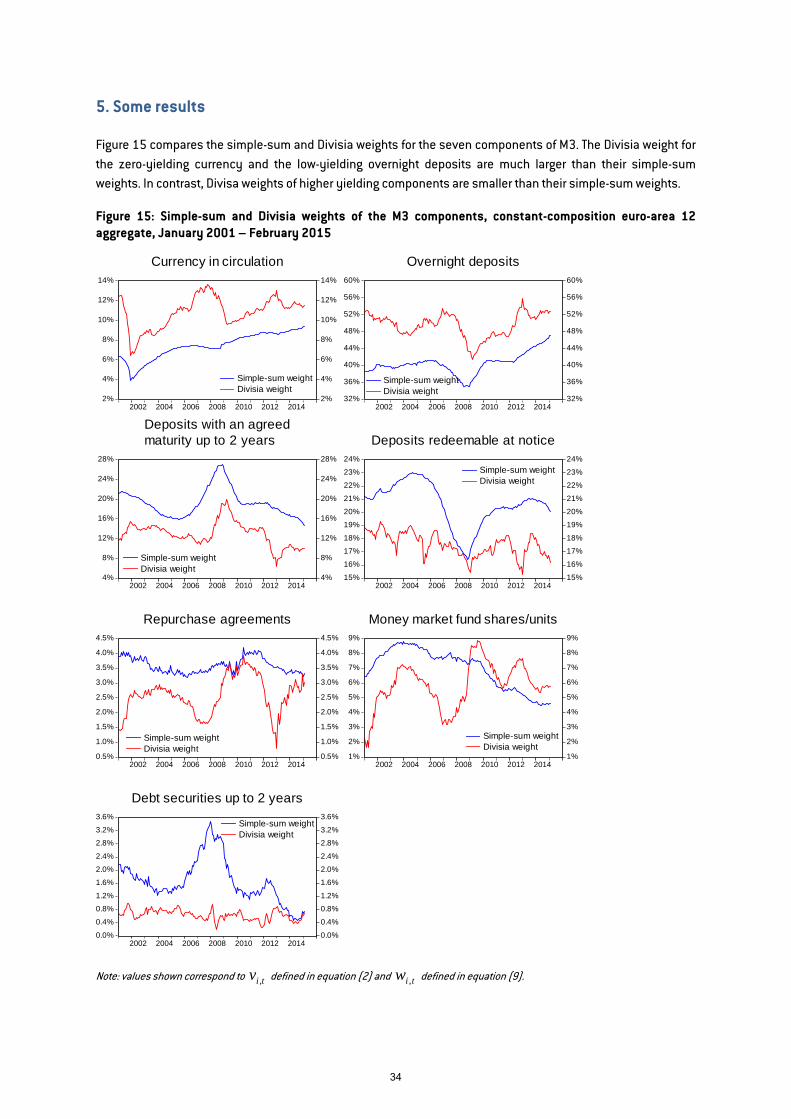
5. Some results

Figure 15 compares the simple-sum and Divisia weights for the seven components of M3. The Divisia weight for the zero-yielding currency and the low-yielding overnight deposits are much larger than their simple-sum weights. In contrast, Divisa weights of higher yielding components are smaller than their simple-sum weights.

Figure 15: Simple-sum and Divisia weights of the M3 components, constant-composition euro-area 12 aggregate, January 2001 – February 2015

2%

4%

6%

8%

10%

12%

14%

2%

4%

6%

8%

10%

12%

14%

2002 2004 2006 2008 2010 2012 2014

Simple-sum weightDivisia weight

Currency in circulation

32%

36%

40%

44%

48%

52%

56%

60%

32%

36%

40%

44%

48%

52%

56%

60%

2002 2004 2006 2008 2010 2012 2014

Simple-sum weightDivisia weight

Overnight deposits

4%

8%

12%

16%

20%

24%

28%

4%

8%

12%

16%

20%

24%

28%

2002 2004 2006 2008 2010 2012 2014

Simple-sum weightDivisia weight

Deposits with an agreedmaturity up to 2 years

15%

16%

17%

18%

19%

20%

21%

22%

23%

24%

15%

16%

17%

18%

19%

20%

21%

22%

23%

24%

2002 2004 2006 2008 2010 2012 2014

Simple-sum weightDivisia weight

Deposits redeemable at notice

0.5%

1.0%

1.5%

2.0%

2.5%

3.0%

3.5%

4.0%

4.5%

0.5%

1.0%

1.5%

2.0%

2.5%

3.0%

3.5%

4.0%

4.5%

2002 2004 2006 2008 2010 2012 2014

Simple-sum weightDivisia weight

Repurchase agreements

1%

2%

3%

4%

5%

6%

7%

8%

9%

1%

2%

3%

4%

5%

6%

7%

8%

9%

2002 2004 2006 2008 2010 2012 2014

Simple-sum weightDivisia weight

Money market fund shares/units

0.0%

0.4%

0.8%

1.2%

1.6%

2.0%

2.4%

2.8%

3.2%

3.6%

0.0%

0.4%

0.8%

1.2%

1.6%

2.0%

2.4%

2.8%

3.2%

3.6%

2002 2004 2006 2008 2010 2012 2014

Simple-sum weightDivisia weight

Debt securities up to 2 years

Note: values shown correspond to tiv , defined in equation (2) and tiw , defined in equation (9).

34

Figure 16 compares the levels and 12-month changes of simple-sum and Divisia M1, M2 and M3 aggregates for our preferred EA12N measure, ie the notional outstanding stocks for the first twelve member states as we calculated from transactions data. For M1 the difference between the two measures is hardly noticeable, but there are some noticeable differences between Divisia and simple-sum measures for M2 and M3. For example, there was an acceleration of money growth in late 2006 and 2007 according to the simple sum measure, but our Divisia measure suggests that there was no major increase in money growth that time. This indicates that while the standard monetary aggregate used by the ECB suggested that inflationary pressures were increasing, this was not the case with our Divisia measure. In 2009, the growth rate of simple sum M3 fell below slightly zero, but our Divisia indicator suggested that money growth remained positive. And in recent months the growth rate suggested by Divisia money is somewhat higher than the growth rate of the simple sum M3, which is good news as Divisia money growth used to predict nominal GDP growth. However, even the most recent money growth rate (February 2015) is below the growth rates observed in the first half of the 2000s so the outlook is not rosy yet17.

17 Our econometric analysis presented in Darvas (2014) underlined that in various structural vector autoregressive (SVAR) models the impulse responses to Divisia aggregates are more sensible and significant than impulse responses obtained when using the simple-sum aggregates.

35

Figure 16: Simple-sum and Divisia monetary aggregates, notional outstanding stocks derived from transactions data, first twelve members of the euro area, seasonally adjusted, January 2001 – February 2015

300

250

200

150

100

300

250

200

150

1002002 2004 2006 2008 2010 2012 2014

M1 DivisiaM1 Simple sum

Levels(January 2001=100)

0

2

4

6

8

10

12

14

0

2

4

6

8

10

12

14

2002 2004 2006 2008 2010 2012 2014

M1 DivisiaM1 Simple sum

12-month change(Percent)

220

200

180

160

140

120

100

220

200

180

160

140

120

1002002 2004 2006 2008 2010 2012 2014

M2 DivisiaM2 Simple sum

0

2

4

6

8

10

12

0

2

4

6

8

10

12

2002 2004 2006 2008 2010 2012 2014

M2 DivisiaM2 Simple sum

220

200

180

160

140

120

100

220

200

180

160

140

120

1002002 2004 2006 2008 2010 2012 2014

M3 DivisiaM3 Simple sum

-2

0

2

4

6

8

10

12

14

-2

0

2

4

6

8

10

12

14

2002 2004 2006 2008 2010 2012 2014

M3 DivisiaM3 Simple sum

36

6. Summary

No official Divisia monetary aggregates are published for the euro area, in contrast to the UK and US. We derive and make available a dataset on euro-area Divisia money aggregates for January 2001 – February 2015 using monthly data and plan to update the dataset in the future.

Academic researchers used to calculate euro-area Divisia indices by using country-specific data and aggregating them to the euro-area level. Since the euro area existed throughout our sample period, we use euro-area-wide components. All necessary data are available from January 2003 onwards and we approximate the four missing interest rate series for January 2001-December 2002.

Our methodology differs from most of the literature in defining the benchmark rate (the return on a monetary asset that does not provide transaction services). Instead of relying on an ad-hoc spread assumption to approximate benchmark rate, we derived the benchmark rate by considering longer maturity bank debts. Our choice has the advantage of not relying on an ad-hoc assumption, but has the drawback that our benchmark asset may not be risk-free, which is an underlying assumption in the particular derivation of the Divisia formula. However, most components of the money stock are not risk-free either and available US and UK Divisia indices are not risk adjusted. We leave risk adjustment for future research.

The euro-area data (monetary aggregates, their components, transactions and interest rates) published by the ECB are changing composition aggregates, ie new euro members are considered from the date of their entry to the euro area. While the member states that joined between 2007-2015 are small, such changing composition aggregates are not suitable for economic analysis. Furthermore, other reclassification changes distort the outstanding stock data published by the ECB, like exclusion central counterparties from repurchase agreements only from June 2010 onwards, leading to a visible break in this series and also in the M3 aggregate. We therefore also derive different versions of euro-area simple-sum and Divisia aggregates, which do not suffer from enlargement-related level shifts and other reclassification changes.

We invite the ECB to publish constant country composition monetary aggregates18. We also encourage the ECB to calculate and publish (constant country composition) Divisia indices.

18 We note that the Eurostat currently publishes four different aggregates for the euro area in its national accounts database: changing composition, euro area 19, euro area 18 and euro area 12.

37

Appendix references

Barnett, William A. (1978) ‘The User Cost of Money’, Economics Letters 1, 145–149

Barnett, William A. (1980) ‘Economic monetary aggregates: an application of index number and aggregation theory’, Journal of Econometrics 14, 11–48

Barnett, William A. (2007) ‘Multilateral aggregation-theoretic monetary aggregation over heterogeneous countries’, Journal of Econometrics 136(2), 457–482

Barnett, William A. and Marcelle Chauvet (2011) ‘How better monetary statistics could have signaled the financial crisis’, Journal of Econometrics 161, 6-23

Barnett, William A. and Neepa Gaekwad-Babulal (2014) ‘Divisia Monetary Aggregates for the European Monetary Union’, paper presented at the inaugural conference of the Society of Economic measurement, Chicago, 18-20 August 2014

Barnett, William A., Douglas Fisher and Apostolos Serletis (1992) ‘Consumer Theory and the Demand for Money’, Journal of Economic Literature XXX, 2086-2119

Barnett, William A., Jia Liu, Ryan S. Mattson and Jeff van den Noort (2013) ‘The New CFS Divisia Monetary Aggregates: Design, Construction, and Data Sources’, Open Economies Review 24, 101-124

Barnett, William A., Yi Liu and Mark Jensen (1997) ‘CAPM risk adjustment for exact aggregation over financial assets’, Macroeconomic Dynamics 1, 485-512

Binner, Jane M., Rakesh K. Bissoondeeal, C. Thomas Elger, Barry E. Jones and Andrew W. Mullineux (2009) ‘Admissible monetary aggregates for the euro area’, Journal of International Money and Finance 28, 99-114

Diewert, Walter Erwin (1976) ‘Exact and superlative index numbers’, Journal of Econometrics 4(2), 115-145

Darvas, Zsolt (2014) ‘Does Money Matter in the Euro area? Evidence from a new Divisia Index’, 6 November, Bruegel Working Paper 2014/12

Divisia, François (1925) ‘L’Indice monétaire et la théorie de la monnaie’, Revue d’Economie Politique 39, 980-1008

El-Shagi, Makram and Logan J. Kelly (2013) ‘Liquidity in the liquidity crisis: Evidence from Divisia monetary aggregates in Germany and the European crisis countries’, Economics Bulletin 34(1), 63-72

European Central Bank (2012a) ‘Manual on MFI Balance Sheet Statistics’, European Central Bank

European Central Bank (2012b) Monthly Bulletin, September 2012

Hancock, Matthew (2005) ‘Divisia Money’, Bank of England Quarterly Bulletin 45 (1), 39-46

Hill, Robert J. (2006) ‘Superlative index numbers: not all of them are super’, Journal of Econometrics 130(1), 25-43

Hulten, Charles R. (1973) ‘Divisia Index Numbers’, Econometrica 41(6), 1017-1026

Jones, Barry E. and Livio Stracca (2012) ‘Does Money Enter into the Euro Area IS Curve?’, unpublished manuscript

38

Reimers, Hans-Eggert (2002) ‘Analysing Divisia Aggregates for the Euro Area’, Discussion Paper 13/02, Economic Research Centre of the Deutsche Bundesbank

Stracca, Livio (2004) ‘Does Liquidity Matter? Properties of a Divisia Monetary Aggregate in the Euro Area’, Oxford Bulletin of Economics and Statistics 66(3), 309-331

Wesche, Katrin (1997) ‘The Demand for Divisia Money in a Core Monetary Union’, Federal Reserve Bank of St. Louis Review, vol. 7, 51-60

39