The World Input-Output Database (WIOD): Contents, Sources and Methods Working Paper Number: 10 Edited by Marcel P. Timmer, with contributions of the WIOD Consortium Members

W o r l d I n p u t - O u t p u t D a t a b a s e

W o r k i n g P a p e r S e r i e s

1

 

 

The World Input‐Output Database (WIOD): 

Contents, Sources and Methods 

 

Edited by Marcel Timmer (University of Groningen) 

With contributions from: 

Abdul A. Erumban, Reitze Gouma, Bart Los, Umed Temurshoev and  

Gaaitzen J. de Vries (University of Groningen)  

Iñaki Arto, Valeria Andreoni Aurélien Genty, Frederik Neuwahl, José 

M. Rueda‐Cantuche and Alejandro Villanueva (IPTS) 

Joe Francois, Olga Pindyuk, Johannes Pöschl and Robert Stehrer 

(WIIW), Gerhard Streicher (WIFO) 

 

April 2012,  Version 0.9

This project is funded by the European Commission, Research Directorate General as part of the 7th Framework Programme, Theme 8: Socio-Economic Sciences and Humanities. Grant Agreement no: 225 281

2

Contents

1. World Input-Output Database: basic contents, set-up and construction philosophy

2. Construction of national Supply and Use tables (SUTs)

3. Sources and methods for Bilateral International Trade data

4. Construction of international Supply and Use tables (Int SUTs)

5. Construction of World Input-Output Tables (WIOTs)

6. Environmental Accounts (EAs): Sources and Methods

7. Socio-economic Accounts (SEAs): Sources and Methods

Appendix Tables

3

1. World Input-Output Database: basic contents, set-up and construction philosophy

The World Input-Output Database has been developed to analyse the effects of globalization on trade patterns, environmental pressures and socio-economic development across a wide set of countries. The database covers 27 EU countries and 13 other major countries in the world for the period from 1995 to 2009. It is downloadable at http://www.wiod.org/database/index.htm.

1.1 Basic contents of WIOD

Broadly, the WIOD consists of time series of

World Tables (annual, 1995-2009)

International Supply and Use table at current and previous year prices, with use split into domestic and import by country (35 industries by 59 products)

World input-output table at current prices and at previous year prices (35 industries by 35 industries)

Interregional Input-Output table for 6 regions (35 industries by 35 industries)

National Tables (annual, 1995-2009)

National supply and use tables at current and previous year prices (35 industries by 59 products)

National Input-Output tables in current prices (35 industries by 35 industries)

Socio-Economic Accounts (annual, 1995-2009)

Industry output, value added, at current and constant price (35 industries)

Capital stock, investment (35 industries)

Wages and employment by skill type (low-, medium- and high-skilled) (35 industries)

Environmental Accounts (annual, 1995-2009)

Gross energy use by sector and energy commodity

Emission relevant energy use by sector and energy commodity

CO2 Emissions modeled by sector and energy commodity

Emissions to air by sector and pollutant

Land use, Materials use and Water use by type and sector

Full lists of the variables covered can be found in the respective sections. The list of countries covered is given in Table 1.

4

Table 1 List of countries in WIOD-database

European Union

North America

Asia and Pacific

Austria Germany Netherlands Canada China Belgium Greece Poland United States India Bulgaria Hungary Portugal Japan Cyprus Ireland Romania South Korea

Czech Republic Italy Slovak Republic Latin America Australia Denmark Latvia Slovenia Brazil Taiwan Estonia Lithuania Spain Mexico Turkey Finland Luxembourg Sweden Indonesia France Malta United Kingdom Russia

1.2 Concept of a world input-output table (WIOT)

In this section we outline the basic concept of a world input-output tables (WIOT) and our approach in construction them. We start with the discussion of a national input-output (IO) table. In Figure 1 the schematic outline for a national input-out table (IOT) is presented. This table is of the industry by industry type. 1 For ease of discussion we assume that each industry produces only one (unique) product. The rows in the upper parts indicate the use of products, being for intermediate or final use. Each product can be an intermediate in the production of other products (intermediate use). Final use includes domestic use (private or government consumption and investment) and exports. The final element in each row indicates the total use of each product. The industry columns in the IOT contain information on the supply of each product. A product can be imported or domestically produced. The column indicates the values of all intermediate, labour and capital inputs used in production. The vector of input shares in output is often referred to as the technology for domestic production. The compensation for labour and capital services together make up value added which indicates the value added by the use of domestic labour and capital services to the value of the intermediate inputs. Total supply of the product in the economy is determined by domestic output plus imports. An important accounting identity in the IOT is that total output by the domestic industry is equal to the use of output from the domestic industry such that all flows in the economic system are accounted for.

[Figure 1 about here]

A world input-output table (WIOT) is an extension of the same concept. The difference with the national tables is that the use of products is broken down according to their origin. Each product is produced either by a domestic industry or by a foreign industry. In contrast to the national IOT, this information is made explicit in the WIOT. For a country A, flows of products both for intermediate and final use are split into

                                                            1 See Miller and Blair (2009) for an elaborate introduction to input-output tables and analysis.

5

domestically produced or imported. In addition, the WIOT shows in which foreign industry the product was produced. This is illustrated by the schematic outline for a WIOT in Figure 2.

[Figure 2 about here]

Figure 2 illustrates the simple case of three regions: countries A and B, and the rest of the world. In WIOD we will distinguish 40 countries and the rest of the World, but the basic outline remains the same. For each country the use rows are split into two separate rows, one for domestic origin and one for foreign origin. In contrast to the national IOT for country A it is now clear from which foreign industry the imports originate, and how the exports of country A are being used by the rest of the world, that is, by which industry or final end user. This combination of national and international flows of products provides a powerful tool for analysis of global production chains and their effects on employment, value added and investment patterns and on shifts in environmental pressures. While national IO tables are routinely produced by NSIs, WIOTs are not as they require a high level of harmonisation of statistical practices across countries. In the following sections we outline our efforts in constructing a WIOT.

1.3. World Input-Output Table (WIOT): Construction Method

In this section we outline the construction of the WIOT and discuss the underlying data sources. As building blocks we will use national supply and use tables (SUTs) that are the core statistical sources from which NSIs derive national input-output tables. In short, we derive time series of national SUTs and link these across countries through detailed bilateral international trade statistics to create so-called international SUTs. These international SUTs are used to construct the symmetric world input-output table which is product or industry based, depending on the set of alternative assumptions used.

The construction of our WIOT has two distinct characteristics when compared to e.g. the methods used by GTAP, OECD and IDE-JETRO. First, we rely on national supply and use tables (SUTs) rather than input-output tables as our basic building blocks. Second, to ensure meaningful analysis over time, we start from output and final consumption series given in the national accounts and benchmark national SUTs to these time-consistent series. SUTs are a more natural starting point for this type of analysis as they provide information on both products and (using and producing) industries. A supply table provides information on products produced by each domestic industry and a use table indicates the use of each product by an industry or final user. The linking with international trade data, that is product based, and socio-economic and environmental data, that is mainly industry-based, can be naturally made in a SUT framework. In contrast, an input-output table is exclusively of the product or industry type. Often it is constructed on the basis of an underlying SUT, requiring additional assumptions.

In Figure 3 a schematic representation of a national SUT is given. Compared to an IOT, the SUT contains additional information on the domestic origin of products. In addition to the imports, the supply columns in the left-hand side of the table indicate the value of each product produced by domestic industries. The upper rows of the SUT indicate the use of each product. Note that a SUT is not necessarily square with the number of industries equal to the number of products, as it does not require that each industry produces one unique product only.

6

A SUT must obey two basic accounting identities: for each product total supply must equal total use, and for each industry the total value of inputs (including intermediate products, labour and capital) must equal total output value. Supply of products can either be from domestic production or from imports. Let S denote supply and M imports, subscripts i and j denote products and industries and superscripts D and M denote domestically produced and imported products respectively. Then total supply for each product i is given by the summation of domestic supply and imports:

j

iD

jii MSS , (1)

Total use (U) is given be the summation of final domestic use (F), exports (E) and intermediate use (I) such that

j

jiiii IEFU , (2)

The identity of supply and use is then given by

iMSIEFj

iD

jij

jiii ,, (3)

The second accounting identity can be written as follows

jIVASi

jiji

Dji ,, (4)

This identity indicates that for each industry the total value of output (at left hand side) is equal to the total value of inputs (right hand side). The latter is given by the sum of value added (VA) and intermediate use of products.

[Figure 3 about here]

In the first step of our construction process we benchmark the national SUTs to time-series of industrial output and final use from national account statistics. Typically, SUTs are only available for a limited set of years (e.g. every 5 year) 2 and once released by the national statistical institute revisions are rare. This compromises the consistency and comparability of these tables over time as statistical systems develop, new methodologies and accounting rules are used, classification schemes change and new data becomes available. These revisions can be substantial especially at a detailed industry level. By benchmarking the SUTs on consistent time series from the National Accounting System (NAS), tables can be linked over time in a meaningful way. In the next section we provide further information about the extrapolation and linking procedures.

In a second step, the national SUTs are combined with information from international trade statistics to construct what we call international SUTs. Basically, a split is made between use of products that were domestically produced and those that were imported, such that

                                                            2 Though recently, most countries in the European Union have moved to the publication of annual SUTs.

7

iEEE

iFFF

jiIII

Mi

Dii

Mi

Dii

Mji

Djiji

,,,,

(5)

where MiE indicates re-exports. This breakdown must be made in such a way that total domestic supply

equals use of domestic production for each product:

iSEFIj

Dji

Di

Di

j

Dji ,, (6)

and total imports equal total use of imported products

iMEFI iMi

Mi

j

Mji , (7)

The outline of an international SUT is given in Figure 4.

[Figure 4 about here]

So far we have only considered imports without any geographical breakdown. To study international production linkages however, the country of origin of imports is important as well. Let k denote the country from which imports are originating, then an additional breakdown of imports is needed such that

iMMEFI ik

kik

Mki

k

Mki

k j

Mkji ,,,,, (8)

The international SUTs for each country are combined into a world input-output table, as given in Figure 2. This transformation step requires additional assumptions that are spelled out in more detail below.

The breakdown of the use table into domestic and imported origin is a crucial step, but empirically hard to make. Ideally one would like to have additional information based on firm surveys that inventory the origin of products used, but this type of information is hard to elicit and only rarely available. We use a non-survey imputation method that relies on a classification of detailed products in the International Trade Statistics, extending the familiar Broad Economic Categories (BEC) classification. Thus we do not rely on the standard import proportionality assumption. Based on this, we allocate imports across use categories in the following way. First, we used the share of use category l (intermediates, final consumption or investment) to split up total imports as provided in the supply tables for each product I across the three use categories. Within each use category allocation is based on proportionality assumption. This generates the import use table. Second, each cell of the import use table is split up to the country of origin where country import shares might differ across use categories, but not within these categories.

It is well known that there are discrepancies between the import values recorded in the National Accounts on the one hand, and in international trade statistics on the other. Some of them are due to conceptual differences, and others due to classification and data collection procedures (see extensive discussion in Guo, Web and Yamano 2009). As we rely on NAS as our benchmark we apply shares from the trade

8

statistics to the NAS series. Thus, to be consistent with the imports as provided in the SUTs we use only shares derived from the ITS rather than the actual values.

Formally, let lkim , indicate the share of use categories l (intermediate, final consumption or

investment) in imports of product i by a particular country from country k defined as

i

lkil

kiM

Mm ~

~,

, such that 1, k l

lkim (9)

where lkiM ,

~ is the total value from all 6-digit products that are classified by use category l and WIOD

product group i imported from country k, and iM~

the total value of WIOD product group i imported by a

country. These shares are derived from the bilateral international trade statistics and applied to the total

imports of product i as given in the SUT timeseries to derive imported use categories. MkjiI ,, is the amount

of product group i imported from country k and used as intermediate by industry j. It is given by:

jI

IMmI

i

jii

Iki

Mkji ,

,,, (10)

where iIIj

jii , such that i

ji

I

I ,is the share of intermediates of product i used by industry j.

Similarly, let f denote the final use categories (final consumption by households, by non-profit organisations and by government). Then the amount of product group i imported from country k and used

as final use category f, MkfiFC ,, , is given by:

i

fii

CFki

Mkfi FC

FCMmFC ,

,,, (11)

The amount of product group i imported from country k and used as investment, MkiGFCF , , is given by:

iGFCF

kiMki MmGFCF ,, (12)

Finally, we derive the use of domestically produced products as the residual by subtracting the imports from total use as follows:

iGFCFGFCFGFCF

iFCFCFC

jiIII

k

Mkii

Di

k

Mkfifi

Dfi

k

Mkjiji

Dji

,

,,,,

,,,, ,

(13)

9

This approach does not necessarily guarantee non-negativity of domestic use values. In those cases when negatives arise, additional constraints are defined through the definition of re-exports such that all values are non-negative (see section on international SUTs).

Note that our approach differs from the standard proportionality method popular in the literature and applied e.g. by GTAP. In those cases, a common import proportion is used for all cells in a use row, irrespective the user. This common proportion is simply calculated as the share of imports in total supply of a product. We find that import proportions differ widely across use categories and importantly, within each use category they differ also by country of origin. Our detailed bilateral approach ensures that this type of information is reflected in the international SUTs and consequently the WIOT.

1.4. World Input-Output Table (WIOT): Implementation of Construction Method

In this section we outline the various steps taken in the construction process of the WIOT. These steps are summarised in Figure 5 that illustrates the basic data sources used and the various transformations applied. Four phases can be distinguished with each different estimation techniques:

A. Raw data collection and harmonisation

B. Construction of time-series of SUTs

C. Construction of import use table and breakdown by country of origin

D. Construction of WIOT

[Figure 5 about here]

A. Raw data collection and harmonisation

Three types of data are being used in the process, namely national accounts statistics (NAS), supply-use tables (SUTs) and international trade statistics (ITS). Importantly, this data must be publicly available such that users of the WIOT are able to trace the steps made in the construction process. Moreover, official published data is more reliable as checking and validation procedures at NSIs are more thorough than for data that is ad-hoc generated for specific research purposes. The data is being harmonised in terms of industry- and product-classifications both across time and across countries. The WIOD classification list has 59 products and 35 industries based on the CPA and NACE rev 1 (ISIC rev 2) classifications. The product and industry lists are given in Appendix Tables 1 and 2. This level of detail has been chosen on the basis of initial data-availability exploration and ensures a maximum of detail without the need for additional information that is not generated in the system of national accounts. The 35-industry list is identical to the list used in the EUKLEMS database with additional breakdown of the transport sector as these industries are important in linking trade across countries and in the

10

transformation to alternative price concepts (from purchasers’ to basic prices, see below).3 Hence WIOD can be easily linked to additional variables on investment, labour and productivity in the EU KLEMS database (see www.euklems.net, O’Mahony and Timmer, 2009). The product list is based on the level of detail typically found in SUTs produced by European NSIs, following Eurostat regulations and is more detailed than the industry list. It is well-known that non-survey methods to split up a use table into imported and domestic, such as used in WIOD (see below), are best applied at a high level of product detail.

To arrive at a common classification, correspondence tables have been made for each national SUT bridging the level of detail and classifications in the country to the WIOD classification. This involved aggregation and sometimes disaggregation based on additional detailed data. While for most European countries this was relatively straightforward, tables for non-EU countries proved more difficult. National SUTs were also checked for consistency and adjusted to common concepts (e.g. regarding the treatment of FISIM (financial intermediation services indirectly measured) and purchases abroad). Undisclosed cells due to confidentiality concerns were imputed based on additional information. The adjustments and harmonisation are described in more detail on a country-by-country basis in Erumban et al. (2012).

B. Construction of time-series of SUTs

As discussed above, national SUTs are only infrequently available and are often not harmonised over time. Therefore they are benchmarked on consistent time-series from the NAS in a second step. From the NAS data time series on gross output and value added by industry, total imports and total exports and final use by use category are taken. This data is used to generate time series of SUTs using the so-called SUT-RAS method. This method is akin to the well-known bi-proportional updating method for input-output tables known as the RAS-technique. This technique has been adapted for updating SUTs and has been shown to outperform other methods for generation of time-series of SUTs (Temurshoev and Timmer 2011).

Timeseries of SUTs are derived for two price concepts: basic prices and purchasers’ prices. Basic price tables reflect the costs of all elements inherent in production borne by the producer, whereas purchasers’ price tables reflect the amount paid by the purchaser. The difference between the two is the trade and transportation margins and net taxes. Both price concepts have their use for analysis depending on the type of research question. Supply tables are always at basic price and often have additional information on margins and net taxes by product. The use table is typically at a purchasers’ price basis and hence needs to be transformed to a basic price table. The difference between the two tables is given in the so-called valuation matrices (Eurostat 2008, Chapter 6). These matrices are typically not available from public data sources and hence need to be estimated. In WIOD we distinguish between margins (including all automotive trade, wholesale trade, retail trade and transport margins) and net taxes on products (taxes minus subsidies). The net tax rates by product are exogenously given, as are the total margins (see section on National SUTs)

                                                            3 In addition, in WIOD the EUKLEMS industry 17-19 is split into textiles and wearing apparel (17-18) and footwear (19) because of the large amount of international trade in these industries.

11

C. Breakdown of import and domestic production in Use table

Our basic data is import flows of all countries covered in WIOD from all partners in the world at the HS6-digit product level taken from the UN COMTRADE database. Based on the detailed product description at the HS 6-digit level products are allocated to three use categories: intermediates, final consumption, and investment.4 This resembles the well-known correspondence between the about 5,000 products listed in HS 6 and the Broad Economic Categories (BEC) as made available from the United Nations Statistics Division. These Broad Economic Categories can then be aggregated to the broader use categories mentioned above. For the WIOD this correspondence has been partly revised to better fit the purpose of linking the trade data to the SUTs (see section on International SUT).

For services trade no standardised database on bilateral flows exists. These have been collected from various sources (including OECD, Eurostat, IMF and WTO), checked for consistence and integrated into a bilateral service trade database. As services trade is taken from the balance of payments statistics it is originally reported at BoP codes. For building the shares a mapping to WIOD products has been applied. For these service categories there does not exist a breakdown into the use categories mentioned above; thus we either used available information from existing import use or symmetric import IO tables; for countries where no information was available we applied shares taken from other countries. (see section on International trade data).

D. Construction of WIOT

As a final step, international SUTs are transformed into a world input-output table. IO tables are symmetric and can be of the product-by-product type, describing the amount of products needed to produce a particular good or service, or of the industry-by-industry type, describing the flow of goods and services from one industry to another. In case each product is produced by only one industry, the two types of tables will be the same. But the larger the share of secondary production, the larger the difference will be. The choice between the two depends on the type of research questions. Many foreseen applications of the WIOT, such as those described in the next sections, will rely heavily on industry-type tables as the additional data, such as employment or investment, is often only available on an industry basis. Moreover, the industry-type table retains best the links with national account statistics.

An IOT is a construct on the basis of a SUT at basic prices based on additional assumptions concerning technology. We use the so-called “fixed product-sales structure” assumption stating that each product has its own specific sales structure irrespective of the industry where it is produced. Sales structure here refers to the proportions of the output of the product in which it is sold to the respective intermediate and final users. This assumption is most widely used, not only because it is more realistic than its alternatives, but also because it requires a relative simple mechanical procedure. Furthermore, it does not generate any negatives in the IOT that would require manual rebalancing. Application of manual ad-hoc procedures would greatly reduce the tractability of our methods. Millar and Blair (2009) provide a

                                                            4 A mixed category for products which are likely to have multiple uses was used as well; this category was allocated over the other use categories when splitting up the use tables.

12

useful and extensive discussion of the transformation of SUTs into IOTs, including a mathematical treatment.

In a first step the international SUTs for all countries are combined into a world SUT. Basically, the national tables are stacked and reordered to resemble a standard supply-use table. Subsequently, using the fixed product-sales structure, the world SUT is transformed into the WIOT given in Figure 2. To ensure consistency between bilateral flows of imports and exports, exports are defined as mirror flows from imports. More specifically, imports of product i of say country A from country B are assumed to be equal to the exports of this product from B to A.

[Figure 6 about here]

The full WIOT will contain data for forty countries covered in the WIOD. Including the biggest countries in the world, this set covers more than 85 per cent of world GDP. Nevertheless to complete the WIOT and make it suitable for various modelling purposes, we also added a region called the Rest of the World (RoW) that proxies for all other countries in the world. The RoW needs to be modelled due to a lack of detailed data on input-output structures. Production and consumption in the ROW is modelled based on totals for industry output and final use categories from the UN National Accounts, assuming an input-output structure equal to that of an average developing country. Imports from RoW are given as as share of imports from RoW from trade data applied to the imports in the supply table. Hence, exports from the RoW are simply the imports by our set of countries not originating from the set of WIOD countries. Exports to RoW for each product and country from the set of WIOD countries are defined residually to ensure that exports summed over all destination countries is equal to total exports as given in the national SUTs. This sometimes resulted in negative exports to the rest of the World. In those cases we added additional constraints to prevent negativity (see section on World Input-Output table).

1.5. World Input-Output Table (WIOT): Basic data sources

As described in the previous section, the construction of the WIOT requires three types of data: national SUTs, National Accounts time series on industry output and final use, and bilateral international trade data in goods and services. In Appendix Table 1 we provide an overview of the SUTs used in WIOD. For some countries full time-series of SUTs are available, but for most countries only some or even one year is available. This is indicated in the table. In some cases SUTs for a particular year were available, but have not been used as they contained too many errors or inconsistencies to be useful. Also, for some non-EU countries SUTs are not available, but only IOTs. For these countries a transformation from IOT to SUT has been made by assuming a diagonal supply table at the product and industry level of the original national table which is often more detailed than the WIOD list. Appendix Table 1 provides details about the size of the original SUTs and IOTs and their price concept. The tables have been sourced from publicly available data from National Statistical Institutes and for many EU countries from the Eurostat input-output database.5

SUTs might be available for various years, but that does not imply that they are also comparable over time as revisions might have taken place in the National Accounts, while the historical SUTs have

                                                            5 These can be found at http://epp.eurostat.ec.europa.eu/portal/page/portal/esa95_supply_use_input_tables/introduction.

13

not been revised. Therefore to link the SUTs over time, National Accounts statistics are used. Data for 1995-2007 was collected for the following series: total exports, total imports, gross output at basic prices by 35 industries, total use of intermediates by 35 industries, final expenditure at purchasers’ prices (private and government consumption and investment), and total changes in inventories. This data is available from National Statistical Institutes and OECD and UN National Accounts statistics. National SUTs are in national currencies and need to be put on a common basis for the WIOT. This is done by using official exchange rates from IMF.

Bilateral international trade data in goods is collected from the UN COMTRADE database (which can be downloaded for example via the World Integrated Trade Solutions (WITS) webpage at http://wits.worldbank.org/witsweb/). This data base contains bilateral exports and imports by commodity and partner country at the 6-digit product level (Harmonised System, HS). Calculations used for the construction of the international USE tables are based on import values. Alternatively, we could have relied on export flow data. However, it is well-known that official bilateral import and export trade flows are not fully consistent due to reporting errors, etc. and hence this choice would make a difference. Following most other studies, we choose to use imports flows as these are generally seen as more reliable than export flows. Data at the 6-digit level often contains confidential flows which only appear in the higher aggregates. These confidential data are allocated over the respective categories. Statistics for trade in goods are well-developed, in contrast to trade in services. Although services trade is taking an increasing share of global trade flows, statistics are only rough and hard to reconcile across the various sources. Therefore trade in services data have first been collected from a number of sources (OECD, WTO, Eurostat, IMF) and based on these a consistent database has been developed. One particular challenge is to allocate the statistics based on Balance of Payments codes to the various products in the WIOD list which has been managed by setting up a correspondence between BoP codes and WIOD product list and applying the respective shares for the country of origin. The approach taken in constructing the bilateral trade data for WIOD is more extensively described in the section on international trade data.

1.6 Socio-economic accounts (SEAs)

In addition to a WIOT, the WIOD also includes socio-economic and environmental satellite accounts. In Figure 6 the conceptual framework of the extended national SUT is given. Value added is broken down into the compensation for the production factors labour and capital. In addition statistics on energy use, greenhouse-gas and other air emissions, and resource use by industry and final users are collected.

[Figure 6 about here]

The socio-economic accounts contain data on detailed labour and capital inputs for all 35 industries. This includes data on hours worked and compensation for three labour types (low-, medium- and high-skilled labour) and data on capital stocks, investment and capital compensation. For labour input, we collected country-specific data on detailed labour inputs for all 35 industries. This includes data on hours worked and compensation for three labour types (low-, medium- and high-skilled labour) and data on capital

14

stocks and compensation. These series are not part of the core set of national accounts statistics reported by NSIs. The database builds upon the data collected in the EU KLEMS project (see www.euklems.net described in O’Mahony and Timmer 2009) by updating it and extending it to a larger set of countries. Within EU KLEMS this type of data is available for about 15 OECD countries up to the year 2007. We extend this data to include also a large set of less developed countries and update to 2009. This extensive coverage of the SEAs in WIOD makes it a unique database compared to what is currently available.

Skills in the WIOD SEAs are defined on the basis of educational attainment levels. Data on number of workers by educational attainment are available for a large set of countries (e.g. Barro and Lee, 2010), but WIOD provides an extension in two directions. First, the WIOD SEAs provide industry level data, reflecting the large heterogeneity in the skill levels used in various industries (compare e.g. agriculture and financial and business services). This has been documented in e.g. Jorgenson and Timmer (2011) for the OECD countries, and this heterogeneity is even stronger in less developed countries. Moreover, the WIOD SEAs also provide relative wages by skill type that reflect the differences in remuneration of workers with different levels of education. The wage data is made consistent with the quantity data and can be used in conjunction to analyse distributional issues such as relative income shares.

Data on wages and employment by skill types are not part of the core set of national accounts statistics reported by NSIs; at best only total hours worked and wages by industry are available from the National Accounts. Additional material has been collected from employment and labour force statistics. For each country covered, a choice was made of the best statistical source for consistent wage and employment data at the industry level. In most countries this was the labour force survey (LFS). In most cases this needed to be combined with an earnings surveys as information wages are often not included in the LFS. In other instances, an establishment survey, or social-security database was used. Care has been taken to arrive at series which are time consistent, as most employment surveys are not designed to track developments over time, and breaks in methodology or coverage frequently occur. For most OECD countries labour data was taken from the EU KLEMS database (www.euklems.org, described in O’Mahony and Timmer 2009), revised and updated. For countries not in EU KLEMS new sources have been used.

The capital data in the WIOD SEAs include investment and capital stocks at current and constant prices. While this type of data is available for the total economy (see e.g. Total economy Database The Conference Board) there is no large-scale database that provides industry level detail. Heterogeneity of capital and investment flows across industries is even bigger than for labour, and taking account of this is crucial in any analysis of the role of capital in structural change and economic growth. The series cover all fixed assets as defined in the SNA 1993. Data on capital stocks is only available up to 2007 unless otherwise indicated. This type of data is available for a limited set of OECD countries in the EU KLEMS database, but not for the majority of the 40 WIOD countries. For the other countries, capital stocks have been constructed on the basis of the Perpetual Inventory Method (PIM) in which the capital stock (K) in year t is estimated as the sum of the depreciated capital stock in year t-1 plus real investment (I) in year t:

Kt = (1-d)Kt-1 +It

with d the depreciation rate. The depreciation rates are taken to be geometric and industry-specific and given in Appendix Table 1. They take into account the differences in the composition of capital assets in various industries and vary from less than 4% in e.g. Education and Public Administration to more than

15

10% in financial and business services. This takes into account the larger share of long-lived assets as buildings and structures in the former, and the larger share of short-lived assets like ICT-equipment and software in the latter. For many countries long time-series of investments are available and there is no need to have information on an initial stock estimate. In cases where investment series were too short, and did not start at least 20 years prior to 1995, an initial capital stock for 1995 had to be estimated.

The section on the SEAs provides more information.

1.7 Environmental accounts (EAs) 6

The core of the environmental database consists of energy and air emission accounts. Energy-related air emissions are estimated using energy accounts and technology-specific emission factors. A large part of the air emissions resulting in the impact categories covered in WIOD (global warming, acidification and tropospheric ozone formation) are originated from gases emitted in energy-use processes. These emissions are complemented with non-energy related (process) emissions where appropriate, using inventory data from reports to the United Nations Framework Convention on Climate Change UNFCCC and CLRTAP (Convention on Long Range Transboundary Air Pollution).

Energy accounts are compiled using extended energy balances from the International Energy Agency (IEA) as a starting point. Additional information was used to bridge between territory and residence principles (adjusting for bunkering and international transport, tourism, defence, embassies) and to allocate IEA accounts to the target classification and accounting concepts consistent with WIOT (e.g. distribution of transport activities and auto-produced electricity among industries). The very first step in deriving energy accounts from international energy balances, as provided by IEA, is to establish a correspondence-key linking energy balance items and NACE entries plus households. Some of the energy balance items can be directly linked to the production of certain NACE entities, but in some cases the energy balance item is related to more than one industry. For instance, the energy balance item “road transport” needs to be distributed over all industries plus households. Likewise, the energy balance item “commerce and public services” needs to be distributed over a number of services. Losses are also a relevant part of the energy accounts and an important element in the assessment of energy efficiency. All losses are recorded and allocated to the supplying industry.

Air emissions are estimated from energy accounts. The general approach implies the use of activity data and emission factors, following the general formula: E = AR× EF. The emission (E) is obtained by multiplying a certain triggering activity (AR: activity rate), e.g. production of the metal industry as measured by output value, by a certain emission factor (EF). Such factors embed the concept of a linear relationship between the activity data and the actual emissions. Several technical guidance documents provide such emission factors, in particular those prepared for the compilation of national emission inventories under international conventions such as United Nations Framework Convention on Climate Change (UNFCCC) and the Convention on Long-Range Transboundary Air Pollution (CLRTAP). Additionally, two very important secondary sources of information for emission factors are

                                                            6 This text is based on the detailed documentation on the environmental accounts by Villaneuva, Genty and Neuwahl (2010) from Institute for Prospective Technological Studies (IPTS) in Seville. IPTS, an EC’s joint research center, is responsible for the environmental accounts in the WIOD project.

16

used: the results of the FP6 project EXIOPOL (http://www.feem-project.net/exiopol/) and the Emission Database for Global Atmospheric Research (EDGAR) information system (http://www.pbl.nl/en/themasites/edgar/ index.html). Activity data will concern the use of energy, broken down into energy commodities and sectors as reported in IEA statistics.

Air emission data not related to energy consumption (e.g. CH4 emissions) will be collected from inventories to complement the energy-based emissions. The substances included in the database comprise the air emissions linked directly to the three environmental impact categories covered, namely:

Greenhouse gas emissions to air (CO2, N2O, CH4, HFCs, PFCs, SF6), needed to derive Global Warming Potentials

Emissions of CFCs, Halons, Methyl Bromide CH3Br, and HCFCs , needed to derive Ozone Depletion Potentials, and

Emissions of acidifying substances to air (NOx, SOx, NH3), needed to derive Acidification Potentials

More detailed information on the construction of the environmental accounts can be found in the section on Environmental Accounts.

The section on the EAs provides more information.

17

2. Construction of national Supply and Use tables (SUTs)

In the WIOD National SUTs are the basic building blocks. Typically, SUTs are only available for a limited set of years (e.g. every 5 year) and once released by the national statistical institute revisions are rare. This compromises the consistency and comparability of these tables over time as statistical systems develop, new methodologies and accounting rules are used, classification schemes change and new data becomes available. These revisions can be substantial especially at a detailed industry level. By benchmarking the SUTs on consistent time series from the National Accounting System (NAS), tables can be linked over time in a meaningful way. We combine NAS data and national SUTs and derive time-series of SUTs using the methodology outlined in Temurshoev and Timmer (2011). In the proces a large number of implementation issues arise. These are being discussed in this section.

Harmonisation and standardisation of national SUTs

The basic building blocks of the WIOT are national SUTs, annual data from the National Accounts and international trade data. The latter is derived from an international source and is discussed in section 4. The SUTs and time series are derived from statistics published by National Statistical Institutes. Although there is increasing international harmonisation of SUT and national account statistics, still differences remain. Also the national data differs in the level of product and industry detail provided. Harmonization involves the following aspects:

Commodity-by-industry classification: National Supply and Use (or Input-Output) ta-bles are converted to 60 products by 35 industries tables. The appendix provides con-cordance tables between national industry classifications, and products and industries (ISIC rev. 3) distinguished in WIOD.

Aggregation levels: the level of industry detail in the basic SUT and I-O tables varied widely across countries, variables and periods. The WIOD consortium has generated a system which allows the comparisons of statistics at various levels of aggregation by using a common commodity and industry hierarchy for all countries.

Reference year for volume measures: countries differ in the reporting of volume measures, e.g. previous year prices vis-à-vis different base years. All series have been put on a 1995 reference year.

Price concepts: the price concept for gross output (basic prices) and intermediate in-puts (purchasers’ prices) have been harmonized across countries. For several countries (including China (producer prices), and India (factor costs)) a different price concept is used. Section 4 outlines how basic price data was obtained on a country-by-country basis.

Other adjustments: For example, differences in the measurement of imports (cif/fob) across countries due to differences in the system of accounts (e.g. SNA 1993 and ESA 1995), and the treatment of FISIM. Approaches differ by country.

For the purpose of WIOT, national data is being harmonised in terms of industry- and product-classifications both across time and across countries. The WIOD classification list has 59 products and 35

18

industries based on the CPA and NACE rev 1 (ISIC rev 2) classifications. The product and industry lists are given in Appendix Tables 1 and 2. To arrive at a common classification, correspondence tables have been made for each national SUT bridging the level of detail and classifications in the country to the WIOD classification.

Harmonisation involved aggregation and sometimes disaggregation based on additional detailed data. While for most European countries (due to a high level of harmonisation of statistics in the European Union) this was relatively simple, tables for non-EU countries proved more difficult. While aggregation of products or industries in a SUT is straightforward, disaggregation is not. To disaggregate an industry first additional data from National Accounts was collected to breakdown value added and gross output by sub-industry. To disaggregate an industry in a supply table, we assumed common product sales shares of the sub-industries. To disaggregate an industry in a use table we assumed common intermediate input coefficients for the subindustries. Disaggregating products is more difficult as additional data by product is often not available. Sometimes a rough estimate could be made based on more detailed industry. Disaggregating products in the supply table is based on common industry-production shares and similarly for the use table we assume common use shares.

National SUTs were also checked for consistency and adjusted to common concepts (e.g. regarding the treatment of FISIM and purchases abroad). In some cases, total supply and total use did not match at the product level, and differences were distributed across the final expenditure categories in order to balance supply and use. Undisclosed cells due to confidentiality concerns were imputed based on additional information.

In particular older SUTs do not have a row allocation for FISIM. If FISIM is not allocated across using industries, value added shares of using industries are used

SUT RAS method for time-series SUTs

SUTs might be available for various years, but that does not imply that they are also comparable over time as revisions might have taken place in the National Accounts, while the historical SUTs have not been revised. Therefore to link the SUTs over time, National Accounts statistics are used. Data for 1995-2009 was collected for the following series:

total exports fob,

total imports cif,

gross output at basic prices by 35 industries,

total use of intermediates at purchaser’s prices by 35 industries,

private consumption at purchasers’ prices

government consumption at purchasers’ prices

gross fixed capital formation at purchasers’ prices

total changes in inventories.

Total taxes minus subsidies

Total margins

19

This data is available from National Statistical Institutes and OECD and UN National Accounts statistics. The national SUTs and the external data from the national accounts is used as input for the SUT-RAS program, but only after total changes in inventories, exports and imports are broken down at the product level (see below). All the data that enters the program exogenously can be found in the so-called SUT Input files that are available from the website (see Table 2.1). This data is used to generate time series of SUTs using the so-called SUT-RAS method. This method is akin to the well-known bi-proportional updating method for input-output tables known as the RAS-technique. This technique has been adapted for updating SUTs and has been shown to outperform other methods for generation of time-series of SUTs (Temurshoev and Timmer 2011). The output of this procedure is given in the national SUTs (see Table 2.2)

Changes in inventories by product

Changes in inventories can be both positive and negative and are highly volatile over time. Including them in the balancing procedure resulted in magnifying of wild swings that are not plausible and heavily affect estimates of the remaining cells. Unfortunately data on changes in inventories by product are typically not collected by NSIs an annual basis. Our alternative is to estimate these based on total changes in inventories as can be found in NAS. We add the change in total changes in inventories pro-rata to the changes in inventories by product as given by the SUTs.

Import and Export data by product

As starting point we use annual data on the total exports and total imports from the National Accounts. For the years for which benchmark supply and use tables are available, the shares by product are taken from these tables and multiplied by the OECD totals to obtain exports/imports by product.7 Between benchmark years the trade data needs to be interpolated. This is based on the international trade statistics (ITS). Interpolation is done using the annual growth rates of ITS. To accommodate the annual fluctuations but at the same time retain the levels in SUT years we employ a procedure which uses the movement of the ITS data minus the average annual growth rate of the ITS data over the considered period. Added to this is the average annual growth rate between the benchmark years.

∗ 2 1 2 1 (14)

Where 1 is the first benchmark year, 2 is the second benchmark year, is the export in year for

product and the export data from ITS at year for product . The ITS data is denoted in dollars,

therefore the growth rate from the ITS data should be adjusted for the growth in the price deflator.

                                                            7 Sometimes we use a division of total exports and total imports into goods and services when given in the National Account Statistics.

20

By using the year to year deviation from the average growth of the ITS data by product and adding this to the average growth between the benchmark years, the ITS imports/exports growth is normalized by product on the average annual growth between the benchmark years. The total of exports/imports over all products still has to be normalized on the OECD imports/exports total for the year under consideration, since the annual OECD growth has not been taken into account in the formula above. Normalizing is done by adding imports/exports over all products, calculating the ratio of this result to the OECD imports/exports total for this year, and dividing all products by this ratio. Thus, this adjustment ratio is uniformly applied to all products.

A problem arises when in one of the surrounding benchmark years exports/imports for the product are zero. In that case they will be zero for all interpolated years. In such cases we can employ the growth rates from the ITS data onto the benchmark year for which the product is non-zero.

Resident and non-resident purchases

Following the SNA standard (chapter 15), final consumption by product in the WIOT refers to consumption expenditure within the domestic market. Thus it includes purchases by non-residents in the domestic territory (such as foreign tourists), and excludes purchases abroad by residents. In order to calculate final consumption expenditure of resident households, it is necessary to add direct purchases abroad by residents and to subtract direct purchases in the domestic market by non-residents. These values are given in separate rows in the WIOT, with balancing values for exports and imports. Ideally, these adjustments should be made at the product level, but the product composition of these expenditures (food, lodging, travel, etc) is typically unknown. So for example, expenditure of foreign tourists on hotels is not recorded as exports of product 55 “hotel and restaurants”, but clubbed with their expenditures on other products in an overall item “purchases by non-residents in the domestic territory”. Similarly, expenditure of foreign travel by residents are clubbed under “Direct purchases abroad by residents”.

Processing trade, re-exports and transit-trade

According to the SNA (following the Balance of Payments Manual, BPM), exports of goods and services consist of sales of goods and services from resident to non-residents, while imports consist of purchases of goods and services by resident from non-residents. This is the change-of-ownership principle. So goods that are in transit through a country (without a change in ownership) are not to be included in export and import statistics. And goods that are imported and exported again without substantial change but did change ownership (so-called re-exports) should be included. However the 1993 SNA recommends one exception to the change-in-ownership principle: goods that are sent abroad for processing (without a change in ownership) and later on re-imported (re-imports) should be recorded gross by the processing economy as well as by the economy that sent the goods for processing, if the processing involves a substantial physical change in the goods (SNA 1993, p.665). From an analytical perspective, these imports should be recorded under intermediate consumption by the processing country, to reflect the underlying technology of the processing industry. This is the concept the WIOT aims for as the input-output table is to reflect the underlying production technology of an industry. However, in practice,

21

countries differ considerably in the application of thi principle due to increasing reporting problems of processing firms. And this has led to the new SNA 2008 recommendation to only record the fee as output and export of a service, and not the flow of intermediate imported goods (SNA 2008, p.279). In practice in the last decade countries differed widely in the treatment of processing trade and this is often not well documented. E.g. in the US IO-tables, re-exports and re-imports are excluded, and also in the Chinese IO-tables parts of imports for processing are excluded both in intermediate inputs and imports. On the other hand, many European countries follow the SNA 93 and record imports for processing as imports for intermediate consumption. Other countries have intermediate positions: in the German IO-tables, both re-exports and imports for processing are included in the export column of the import matrix but not in intermediate consumption block. The WIOT is constructed following the SNA 93 convention such that the intermediate use of an industry best reflects the underlying production technologies (e.g. a wearing apparel firm sewing shirts should be represented by an intermediate flow of cloth and output flow of shorts, instead of no intermediates and the processing fee as output only). We add back re-exports and re-imports when this is needed, and possible, notably for the US and China. For these countries some re-xports were added back into the original input-output table.

In the US National Income and Product Accounts (NIPA), following the SNA, re-exports are included in foreign trade value. But in the IO-accounts, “re-exports”, defined as “goods produced outside the US, previously imported in substantially the same condition”, are excluded. (BEA, 2009, Concepts and Methods of the U.S. I-O accounts, p. 7-7)). Clearly, the BEA IO- accounts have a stronger definition of “substantially different” than the NIPA. Based on the gross export and re-export statistics reported in the UN COMtrade database, estimates for re-exports by product were made and added to both export and import value to maintain consistency. The amount of re-exports has been steadily increasing from 7 to 13% of total net goods export between 1995 and 2005, and was up to 50% or more in the late 2000s for goods like machinery (29), electronics and parts (30 and 32), and other manufacturing (36, mainly jewellery). Another important adjustment to be made to the US SUTs was the allocation of the row called “non-comparable imports”. Intermediate use of non-comparable imports consists mainly of business services (REF!! ) and have been allocated to good 74 (Other business services nec). Final use of these imports are allocated to WIOT row “Direct purchases abroad by residents”. The rest-of-the –world adjustment to final use was allocated to WIOT row “Purchases on the domestic territory by non-residents” (BEA 2009, chapter 7). Finally, all negative entries in the import-column in the BEA Use table are allocated to the WIOT-row “Cif-fob adjustment on imports” to conform the WIOT concepts. Tables for 1995-1997 have been extrapolated in the standard way based on NIPA series for industry output and final use, but using UN COMTRADE to extrapolate imports and exports of goods at the product level from their 1998 level.

Price concepts and margin tables

Timeseries of SUTs are derived for two price concepts: basic prices and purchasers’ prices. Basic price tables reflect the costs of all elements inherent in production borne by the producer, whereas purchasers’ price tables reflect the amount paid by the purchaser. The difference between the two is the trade and transportation margins and net taxes. Both price concepts have their use for analysis depending on the type of research question.

22

Supply tables are mostly at basic price and often have additional information on margins and net taxes by product. The use table is typically at a purchasers’ price basis and hence needs to be transformed to a basic price table. The difference between the two tables is given in the so-called valuation matrices (Eurostat 2008, Chapter 6). These matrices are typically not available from public data sources and hence need to be estimated. In WIOD we distinguish between margins (including all automotive trade, wholesale trade, retail trade and transport margins) and net taxes on products (taxes minus subsidies). The net tax rates by product are exogenously given derived from the supply tables. In the SUT-RAS process they are retained to the extent possible. The margins are derived residually in the following way, in two steps:

First, within the SUT-RAS procedure we compute a vector of the sum of trade and transport margins and net taxes on products. In this stage the following components of margins and net taxes (coming mainly from national accounts sources) are taken exogenously:

‐ The total value of all margins and net taxes (a scalar), and ‐ The exact values of three trade margin products and four transport margin products, which are

taken exogenously similar to the vectors of products’ exports, imports and changes in inventories. In the second stage, the first step output as to be separated into two vectors of total margins and net taxes. At this stage the following data is taken exogenously:

‐ Rates of net taxes by product; these are derived from the original national SUTs by dividing products’ net taxes by the corresponding total supply at purchasers’ prices,

‐ The value of total net taxes (a scalar). It should be noted that we could have endogenized separately wholesale, retail and motor trade margins and net taxes within the SUT-RAS procedure (which was the case), but later it was decided to estimate these altogether in one vector, and then use the tax rates from the national SUTs to derive the net taxes on products so that these rates are kept in the final estimates. Let us denote the derived value of total margins and net taxes of product i by (which is the output of the above mentioned first step) and its exogenous tax rate by . Then the estimate of net taxes of product i, , is derived as

Υ 1 Υ , (1) where is the derived value of total supply of product i at purchasers’ prices and Υ is an indicator function which equals 1 when product i has positive margins and 0 otherwise. That is, some products have no margins (these are mainly services), hence the derived value of margins and net taxes, should be defined to be the net taxes for such products. For other products, we apply the net tax rates to the estimated total supply to get the corresponding net taxes. That is, what eq. (1) does. Denote the exogenous value of total taxes by . We now must normalize ’s from (1) such that ∑ . This normalization is derived from

1 Υ Υ ∑ 1 Υ   / ∑ Υ , (2) which are used as the final estimates of net taxes for product i. Note that in (2) normalization is applied to initial net taxes of products with positive margins only (we cannot change those for products without

23

margins, because the remaining values cannot be allocated to margins that should be zero by construction). The residual, ≡ , is then defined as total trade and transport margins of product i. The tables of margins and net taxes are computed from derived and . This is done, first, by computing the new margins and net taxes rates. These are computed simply by dividing both and

by the corresponding total supply excluding exports, . Then these rates are multiplied row-wise by the purchasers’ price Use table components, except exports. These calculations give us the tables of margins and net taxes, respectively. These tables are given in the national SUT files.

Exports and imports valuation

Exports are valued at free-on-board (fob) prices at the border of the exporting country. Imports are valued at the cost-insurance-freight (CIF) price at the border of the importing country before import tax, so they include international transport and insurance services. As part of these services might be carried out by a resident producer, and hence is already recorded as output of the domestic economy, double counting might arise. In the SNA 1993 this is corrected by a cif/fob adjustment on imports. Countries differ in the way this adjustment is calculated and recorded in their SUTs, and specifically the European system of Accounts (ESA 95) suggests an alternative different from the SNA. We follow the European system of recording in which there is a cif/fob adjustment on imports, mirrored by a similar adjustment value on exports to maintain balance in the system. They are the same by construction, for further discussion see, Eurostat (2008). Typically, this adjustment is minor.

Deflation of SUTs

SUTs are also derived at previous year prices. Deflation is done by deriving product level deflators based on industry gross output deflators, through weighting with the productshares from the supply table. More specifically, we prepare price indices for each cell in the S and U matrix. Second, we deflate all elements and aggregate to arrive at total intermediate inputs and final demand at previous year prices.

The deflator for each cell in the S matrix is set equal to the price index of the producing industry. We then derive a Paasche price index for domestic supply of each commodity on basis of supply table. The commodity deflator is a weighted sum of the price indices of the supplying industries. Weight are the market shares (industry shares in total domestic supply of the commodity) in current year (Paasche price index).

Second, we set price deflator for each commodity in the Use table at basic prices as domestic price index for domestic supply derived above. To Deflate SUT to previous year prices we divide the nominal SUT for year t by the price indices derived in the previous steps. Thus we derive a chained Laspeyres quantity measure. Calculate total intermediate input and final demand as the sum over the commodities (column wise). We deflate gross output in the U by the price index for each industry and define value added as gross output minus intermediate inputs for each industry. This value added is now double deflated and may not correspond to the value added at constant prices as given in the SEAs

24

To deflate Cif/ fob adjustments on exports, Direct purchases abroad by residents, Purchases on the domestic territory by non-residents we used the GDP deflator

Table 2.1 Example of SUT input file

Country Australia Time series SUT Input data Source: WIOD database, January 2012 release

Tables Description SUTs Availability table for benchmark SUTs Output Gross output by industry at current basic prices (in millions of national currency) UseTotals Intermediate and final use totals at current basic prices (in millions of national currency) Deflators Price levels of Industry gross output and GDP as ratio of previous year Exports Exports by product and adjustment items (in millions of national currency) Imports Imports by product and adjustment items (in millions of national currency) InvChanges Changes in inventories by product (in millions of national currency) NetTaxesRates Net tax rates by commodity (as % of total use at purchasers' prices minus exports) Margins_Tax Trade and transport margins and net taxes (totals in millions of national currency) SUP96 Official supply table for 1996 SUP03 Official supply table for 2003 SUP04 Official supply table for 2004 USE96 Official use table for 1996 USE03 Official use table for 2003

Table 2.2 Example of National SUT file

Country Australia Time series Supply and Use tables Source: WIOD database, January 2012 release

Tables Description SUP_bas Supply tables at basic prices USE_pur Use tables at purchasers' prices USE_bas Use tables at basic prices Margins Margins NetTaxes Net taxes SUP_pyp Supply tables at previous year prices USE_pyp Use tables at previous year basic prices

25

3. Sources and methods for Bilateral International Trade data

3.1 WIOD international trade in goods data

Introduction

This section describes the construction of the international trade data in goods used in the WIOD project (for a more detailed outline see Pöschl and Stehrer, 2012). The bilateral trade data serves two reasons: First, these should allow for a split of imports (and exports) into end-use categories and, second, to provide information on the bilateral flows of products split up by end-use categories across countries. Both types of information have to be applied to split import use tables from total national use tables. First, an overview over data sources and correspondences applied is given. Second, treatment of particular arising data issues concerning confidentialities, missing information, and country specific problems are reported. It should be noted that information from the trade data used for construction of the international supply and use tables system are the shares by end-use categories and bilateral trade flows applied to the levels of imports and exports provided in the national supply and use tables.

Data sources

The raw data was taken from the UN Comtrade (http://comtrade.un.org/db/default.aspx) and downloaded at the HS 6-digit level. The trade database contains the 40 WIOD countries over the period 1995-2010 as reporter countries and all other countries as partner countries. Additionally data for Hong Kong and Macao has been used to improve trade data on China. Most countries are in HS 1996 from 1996-2010 and HS 1992 for 1995. Due to a lack of HS 1996 data, several countries however also report in HS 1992 for 1996 (Brazil, Latvia, Lithuania, Romania, Russian Federation, Slovakia).

In some cases trade data are missing. We therefore filled some gaps with data obtained from other sources: exports of Denmark and Czech Republic in 1997 from the OECD8 and 1995 trade data for Bulgaria directly from the National Statistical Institute of Bulgaria. Unfortunately, it was not possible to get Russian trade data for the year 1995 as the Federal Customs Service of Russia only has data from 1996 onwards.

Confidentiality issues

Having thus collected the raw data, in a next step confidentiality issues has to be tackled. Confidentiality issues arise when firms in a country do not want to report either which amount of a certain product they have been trading (product-related confidentials) or with whom they have been trading (partner-related confidentials). This is allowed when there is a nearly monopoly situation for a specific product in a country. Whenever firms do want to conceal their trade destination, the trade flow ends up in an artificial partner country "Special Categories" or "Areas, nes". Such trade flows which might be included in the

                                                            8 We would like to thank Colin Webb, Norihiko Yamano and Shiguang Zhu from OECD for their efforts and help in obtaining the necessary data.

26

information on imports and exports in the national supply and use tables might result in a distortion of bilateral trade flows. Since it is not possible to directly assign such flows the following procedure was applied. Trade with partners "Special Categories" and "Areas, nes", where trade is broken down by HS 6-digit codes, have been distributed to the trade values among the other partner countries according to the difference between total trade reported and the sum of HS 6-digit codes. This is possible since trade not reported at the HS 6-digit level will be partly included in the total trade value.9 Confidential products in the UN database end up in categories like "999999 Commodities not specified according to kind" or "9999AA Commodities not elsewhere specified" in order to conceal the underlying products traded. These products could not be aligned with industry categories and are therefore not considered in the construction of international supply and use tables.10

Country-specific problems

There are also some problems specific to some particular countries which have to be handled separately. There are two particularly thorny issues related to China’s trade data. First, data for trade with Taiwan does not exist in the UN Comtrade. Second, the special administrative regions (SAR) of China, Hongkong and Macao are reported separately in the trade data. We have handled China and the SAR using as one economic entity. Therefore China as a reporter and partner therefore includes the trade values of other countries with China, Hongkong and Macao consistent with the values reported in the Chinese national supply and use tables. Flows between China and the SARs have been dropped as well as re-imports and re-exports.

Concerning Taiwan, the following statement can be found at the UN website (http://comtrade.un.org/kb/article.aspx?id=10223): “As a partner, code 490 (Other Asia, nes) contains Taiwan and other unknown countries in Asia. In practice, Code 490 can be assumed for Taiwan, except for several countries (such as Saudi Arabia which report all of their exports to unknown countries).” We further checked whether there are other countries not covered by the UN Comtrade which might be included in this aggregate and found the following countries with most likely negligible trade volumes: Nagorno-Karabakh Republic, Christmas Island, Palestina and South Ossetia. Some countries might still report trade with the partner "Other Asia, nes" for confidentiality reasons but it should be fine for most WIOD countries. For Taiwan as a partner we therefore used the reporter countries’ trade with "Other Asia, nes". Trade data for Taiwan as a reporter was obtained from OECD which collected data for Taiwan.

International trade statistics report the Belgium–Luxembourg Economic Union (BLX) as a combined entity until 1999 when European Community rules required splitting this information. We observed that at the NACE 3-digit level, trade values seem to be pretty much stable and no large restructuring is noticeable in the data. We therefore calculated the average shares of trade values and quantities for 1999-2000 and 2000-2001 at the NACE 3-digit level for Belgium and Luxembourg separately. These shares we applied backwards on the combined trade of the Belgium–Luxembourg Economic Union for 1995-1998. The methodology was applied for BLX as a reporter and partner. In order to construct the trade between

                                                            9 See UN Comtrade readme http://comtrade.un.org/db/help/uReadMeFirst.aspx. 10 In the underlying trade data which are available from the WIOD website these are included as a separate industry code.

27

Belgium and Luxembourg, which is not reported by BLX as well, we used a similar approach. For each of the two countries we calculated the average of the growth rates of trade values and quantities for 1999-2000 and 2000-2001 at the NACE 3-digit level. Due to large fluctuations for small sectors, the growth rate was set to 1 (no growth) for values smaller than 50.000 euro at the NACE 3-digit level. These growth rates we applied backwards to each country’s trade in 1999 in order to construct the bilateral trade data at the NACE 3-digit level.

Correspondence to end-use categories and products

Starting from HS 6-digit which provides information on bilateral flows of goods of about 5000 products, the individual flows were merged with a correspondence of the HS 6-digit products to use categories distinguishing “Intermediate consumption”, “final consumption”, and “capital goods”. This correspondence was constructed from the Broad Economic Categories (BEC revision 3) classification as provided by UN and the correspondence between these detailed end use categories into broader groups as applied by OECD (see Appendix Table 4). For a number of products the correspondence to a particular use category was however revised by reclassifying products to the above mentioned three categories. About 700 products have been reclassified by this procedure though in many cases these products have only relatively low shares in overall trade and therefore might not be visible in overall descriptive but might play a role for particular bilateral flows. On top of that reclassification there still exist the problem that one particular good might qualify for two use categories. For example, cars might be considered as final consumption or investment good and motor spirits might be use as intermediate inputs or final use by consumers. Therefore, weights have been applied each product at the HS6-digit level allowing for a classification into the three end use categories “Intermediate consumption”, “Final consumption” and “Gross Fixed Capital Formation”.11 Furthermore, the HS 6-digit data was merged with a correspondence to NACE revision 1 at the 2-digit level as made available by Eurostat corresponding to the CPA classification in the national supply and use tables.

Summary

This provides a consistent set of bilateral trade in goods data for the 40 WIOD countries and a rest of world category at the level of products consistent with the national supply and use tables over the period 1995-2009. Furthermore, these flows are split by end-use categories allowing the construction of international supply and use tables without using the proportionality assumption, i.e. allowing to take account of the fact that a country’s geographic structure of imports differ by use category.

                                                            11 The weights applied in most cases have been 50:50 though in some cases we put different weights. The applied correspondence is available at www.wiod.org.

28

3.2 WIOD international trade in services data

Introduction

In this section we report on the construction of the bilateral data on services flows across countries to serve as an input in the construction of the international supply and use tables. Services have unique characteristics that greatly affect their tradability. The two most obvious characteristics include intangibility and non-storability, however typically they also require differentiation and joint production, with customers having to participate in the production process. In order to capture these aspects and to allow for trade in services that also require joint production, the WTO defines trade to span four modes of supply:

Mode 1 – Cross-border: services supplied from the territory of one country into the territory of another.

Mode 2 – Consumption abroad: services supplied in the territory of a nation to the consumers of another.

Mode 3 – Commercial presence: services supplied through any type of business or professional establishment of one country in the territory of another (i.e., FDI).

Mode 4 – Presence of natural persons: services supplied by nationals of a country in the territory of another.

In the dataset collected only data on cross-border services trade in GATS modes 1 and 2 can be collected due to data limitations as these are reported in the Balance of Payments statistics. Though these are also the categories needed for the purpose of constructing international supply and use tables one should be aware that FDI remains an important channel for foreign providers to supply services. About 60% of global FDI stock is in the service sector, with finance and trade being the most important sectors therein. Services are also traded through cross-border movement of persons. On the consumer side (GATS “mode 2” trade), this includes for example Germans and Irish going to Poland for dental work, as well as tourism. On the producer side (GATS “mode 4” trade) it includes the cross-border temporary movement of skilled labour, like accountants and software engineers who increasingly work across Europe. It also includes Polish construction workers relocating temporarily for jobs in the Netherlands and France.

Data sources and compilation

To create a data set covering bilateral services flows data from the OECD, Eurostat, UN, and IMF data (the latter data are only on trade with the World as a partner) have been collected. OECD, Eurostat and UN provide data on bilateral services trade flows on dual breakdown, by partners and BoP codes. The most comprehensive coverage of reporting countries among the three sources is UN, which provides data on 190 reporters. Eurostat and OECD provide data for a limited number of reporters: Eurostat covers 27 EU members plus Croatia, Iceland, Japan, Norway, Turkey, Switzerland, and USA; while OECD covers 28 countries (all the OECD members apart from Chile, Iceland, Israel, Slovenia, and Switzerland). Time coverage is the biggest in EUROSTAT, which reports data starting from 1995. IMF data cover 166 reporters and 28 sectors for the period 1995-2008. WTO data on services trade have not been included

29

since they provide limited coverage of sectors and partners – the data are reported only for 3 sectors and for World as a partner. Since the quality of existing services data is rather low as compared with merchandise trade statistics, the data have to be adjusted extensively to assure their consistency.

Working with multiple sources makes it somewhat easier to identify problems in the data linked to human error. For example, there are clear cases where data were entered such that one source reports flows three orders of magnitude above the other two sources for the same flow. Based on examination of the data, comparisons across sources have been made to filter errors of this type, as well as other problems apparently linked to identifiable data entry errors. 12 It is also clear in examining the data that UN sources have in many cases identified and cleaned up errors that remain in the EUROSTAT and OECD series. In other words, they have identified and corrected many of the errors, like scaling problems, which we can also spot in the data. For this reason, the following database construction rule was applied:

the preferred source data is United Nations data;

the second source is mirrored UN data (i.e., we use mirrored UN data only in cases when no UN data are available for a given data point);

the third preferred source is Eurostat corrected (meaning after we fix identifiable magnitude problems) (i.e., we used Eurostat data only in cases when no UN data or UN mirrored data are available for a given data point);

the fourth preferred source is Eurostat mirrored (again corrected);

the fifth source is OECD;

the sixth source is mirrored OECD data.

In total, mirror flows accounted for 31% of all non-missing observations. For situations where a value of an aggregate was lower than the sum of its parts (trade values for some sectors were lower than the sum of values of their subsectors, or trade with the World was lower than the sum of trade flows to individual partners) adjustments have been made. In such cases we changed the value of an aggregate by the difference between its initial value and sum of its components. Further, a code 999 was created to account for bilateral trade flows which were not allocated in terms of sectors (i.e., when sum of trade across all sectors was smaller than total services trade for a given country pairs and year). About 6% in the final dataset of all the observations fall into this category (also around 6% in terms of total trade value).

We have also mapped bilateral data on flows against data on total flows. This allows the addition of a region "XWD" which holds unallocated imports and exports for each country. Of course, where we have no data to begin with, this does not help. With the addition of the XWD region, bilateral and aggregate data are internally consistent, including mappings from the aggregate to bilateral databases. As noted above, tf reported bilateral flows exceed reported totals, we go with the constructed totals. The flows with the "XWD" follow from comparing total identified bilateral flows to reported total flows. Where the bilateral sums exceed reported totals, there is no "XWD" residual. This is usually the case if we have no

                                                            12 OECD data have a number of suspicious spikes and jumps which we believe are most likely linked to human errors during data entry. Eurostat data suffered in some cases from a magnitude problem: some values of trade reported by the Eurostat were apparently in thousands of USD rather than in millions. In both cases, this may follow from compatibility problems with conventions for CSVand TSV file formats.

30

reported totals, but only mirror bilateral flows. Often, there are unreported bilateral flows, so that total exports and imports with world imply unallocated flows. These unreported flows are with the partner "XWD". Given XWDn as a partner, we can use the bilateral flow data to then map total flows to total flows from the i-o tables. XWD is both an importer and exporter, so summing bilateral across partners gives total imports, and summing the flows over reporters gives total exports. In both cases these correspond to the "trade with world" values.

Coverage

The dataset contains data on bilateral services trade flows for the 40 WIOD countries as reporters and partners plus a rest of world. Additionally, data for each of the countries with trade with the world is available. Data are reported in million US-$ for 1995 – 2009. The coverage by BOP classification is presented in Table 3.1. The data include more than 20 economic activities according to the BOP classification. However, not all sectors have the same coverage in terms of time and trading countries. In general, the higher the level of disaggregation, the fewer observations are available.

As a word of caution it should be added that the quality of trade data in services is still far away from being comparable to trade data for merchandise goods. Due to the long tradition of tariff revenues, trade data for goods have been collected with quite high quality and accuracy. Due to intangibility and non-storability of services, at-the-border-duties cannot be applied to services, thus having resulted in much weaker compilation practices with considerable less accuracy. Thus, services statistics has ample space for improvement in terms of measurement. In particular with respect to modes 3 and 4, measurement is up to date difficult and incomplete. Ongoing revisions and refinements of the BOP classification work towards solving these issues. The WIOD Trade in Services Database should be seen in this light as the best currently available approximation to a comprehensive picture of global trade flows in services.

31

Table 3.1 – Service sector classification by BOP categories

200: Total services

205: Transport

236: Travel

240*: Other Commercial Services (200-205-236-999)

245: Post and telecommunications

246: Post and courier

247: Telecommunications

249: Construction

253: Insurance

260: Financial intermediation

262: Computer and information

264: Information services

266: Royalties and license fees

268: Other business services

269: Trade and repairs

272: Renting machinery and equipment

273: Miscellaneous business, profession

274: Legal, accounting, professional

275: Legal

276: Accounting, auditing, bookkeeping

277: Business and management consulting

278: Advertising, marketing, polling

279: Research and development

280: Architecture, engineering, technical

282: Waste treatment and de-pollution

284: Other business services

286*: Unallocated other business services

287: Personal, cultural, recreational

291: Government services

999*: unallocated bilateral trade flows

* We created these sectors. The EBOPs includes additional sectors, though usually without data.

32

4.Construction of international Supply and Use tables (Int SUTs)

Introduction

The next step is to combine the national (total) supply and use tables (NatSUTs) with the information on bilateral trade by use categories from the trade data to construct international supply and use tables for each country. Basically, this means, first, to split out import use tables from the national total use tables. The benchmark for total imports by product stems from the import column in the supply table. It is important to note that imports are reported in cif terms. These imports can either be used as intermediates or as final consumption, with the latter split into household consumption and gross capital formation with the various subcategories. We refer to these as “use categories”. Trade in goods data allow to split imports into these three categories as described in the section on trade data. For trade in services a particular assumption had to be made as described below. Within these three use categories a proportionality assumption for each of the respective more detailed categories has to be taken resulting in an import use table. Further information from data then allows, second, to split each cell of this import use table by country of origin. It should be noted that the geographic sourcing structure therefore differs by product and use category (though the same sourcing structure is applied for each item within a use category). This already results in an import use table split by country of origin. As this is however in cif terms (note that the procedure started from the imports in cif terms as provided in the supply table) international trade margins have to be subtracted for each bilateral flow. This then results in the import use table from which the world SUTs and WIOTs can be achieved.

Though in general, this procedure is relatively straightforward, there are many details to be accounted for to arrive at a consistent international SUT for each country. The various steps are now discussed in more detail.

Exchange rates

The construction of the international supply and use tables started with a conversion into current US-$. The exchange rates applied were collected from the International Financial Statistics Database (IFS) according to the currencies in which the national supply and use tables were reported. This resulted in a set of 40 national supply and use tables for each year over the period 1995-2009 at current US-$ (expressed in mn US-$). The decision to convert them into US-$ was motivated by the fact that trade statistics are as well reported in US-$ terms. For the Euro-zone countries particular care was taken as these countries report national accounts before introduction of the euro in euro-fixed exchange rates. These have been converted by using the US-$ per national currency exchange rate adjusted to euro-fixed (i.e. divided by the fixed conversion factor).

International trade and transport margins and rest-of-world

The construction of the international SUTs then proceeded in various steps. The supply tables (at basic prices) report total import flows for each in cif terms whereas the use tables (as well in basic prices) report total exports by product in fob terms. As the respective import blocks in the international use tables should be in fob terms (note that the rows provide information on exports of other countries to the

33

reporter country) to be compatible with the export column in the use tables, imports have to be converted into fob terms.

This requires estimations of bilateral trade margins by product category. This is in detail outlined in Streicher (2012) of which a summary is provided here. Based on the detailed trade data from the UN COMTRADE database which additionally provides information by import quantities a gravity type model was estimated with the ratio of import unit values and export unit values as dependent variable and gravity variables (distance, landlockedness, dummy for same continent) as explanatory variables. In these regressions not all bilateral flows could be taken into account as the UN COMTRADE does not report all quantities in kg (but also in other units). Additionally, mirror flows in quantities often too not match only observations of which recorded quantities of the mirror flows deviated with less than +/-5%. Further, estimations were restricted to flows whose cif-value was larger than its fob-mirror. (Though this should hold by definition it is not the case in about a quarter of flows.) From various specifications (see Stehrer and Streicher, 2012b) which have been tested results in a bilateral set cif-fob ratios which tended to be larger when compared to results in the literature due to restriction of the sample. This was partly taken into account by allowing for squared distance and subtracting the resulting cif-fob margins for neighbouring countries (which theoretically should be zero). This resulted in a set of bilateral cif-fob margins for each CPA product. These were set to zero for neighbouring countries. For trade in services there is no distinction made between cif and fob flows.

The resulting international trade and transport margins from these cif-fob ratios and the bilateral flows based on trade data have further been benchmarked by the trade balance of the WIOD countries in the margins sectors (transport and trade). The logic behind as outlined in Streicher and Stehrer (2012) is that such services has to be produced somewhere and thus are reported in the supply tables but are not reported as consumed in the producing country and are imported in any other country if form of goods reported in cif. Thus, all WIOD countries should run a surplus in these products which is actually the case with the surplus being about 5-6% of total manufacturing imports of WIOD countries. Benchmarking the bilateral trade and transport margins to these surpluses, result on overall transport costs of 5-7% of imports on average. Of course, the resulting bilateral margins very much depend on the country-pair and the respective product. Further implicit assumptions are that the bilateral cif-fob ratios are symmetric for each country-pair and product13 and the same across use categories.

The rest of world has not to be modelled explicitly in case of the international SUTs by country. The additional block in the international use table of imports from rest-of-world results from the shares of imports from ROW in the bilateral trade data, i.e. these are the imports which are not sourced from other WIOD countries. Note, that exports to rest-of-world result in a later stage as the difference between exports of WIOD countries to other WIOD countries and the overall exports of this country as reported in the use table.

The version of the international SUTs (those reported on the web) are based on these benchmarked bilateral cif/fob margins from the estimations which were applied to each bilateral flow for all manufacturing products. Adding up the resulting bilateral transport costs by partner for each product and subtracting them from the import values in cif terms from the supply tables result in imports in fob terms for each country and product. This information is reported in the international supply tables as an extra

                                                            13 Results were also derived with asymmetric cif-fob ratios which might result from the structure of detailed products within each 2-digit category. However, in the procedure of constructing international use tables only we used the average of these ratios.

34

column. Furthermore, the information from bilateral import flows in fob terms provides respective shares for each country’s total imports by partner and product. This automatically scales the information from trade data to the levels as provided in the supply tables.

The above described procedure however might result in negative exports of a country to the rest-of-world as exports are defined as mirror flows and the total level of a country’s exports is given by the information in the national use table. For construction of the analytical WIOTs therefore a reporter “Rest of the world” (ROW) was created. The world aggregate of exports and imports at the HS 6-digit level was downloaded from the UN COMTRADE to which the same adjustment methods as for the other reporter countries have been applied. Subtracting the other reporters from this world aggregate yields exports and imports of ROW. Data for trade in services have been available anyway in the WIOD TiS database. Similar to above imports in fob terms have been derived. As the information on exports and imports from the national SUTs dictate the trade surplus and deficit of all WIOD countries with respect to ROW by product the levels of exports and imports of ROW has to be adjusted to obey this constraint. This provides a bilateral trade matrix and total imports and exports for each product for all WIOD countries and ROW. This was used as the starting point for the RAS procedure to arrive at a consistent bilateral trade matrix with total exports and imports in line with the information from the national supply and use tables. These adjusted trade data have then been used to construct the international supply and use tables following the steps reported above.

Definition of re-exports and additional assumptions

For constructing the international use table for a country some further assumptions had to be taken: First, it was assumed that changes in inventories are only sourced from domestic production. Similarly, exports can only be sourced from domestic production (for definition of re-exports see below). Finally, it was secured that eventual arising negatives in the intermediate use or final demand blocks of the national tables are not considered when calculating the international use blocks. The reason for this is that when applying shares by country of origin negative entries would appear in the forty other blocks of a country’s international use table. Thus any remaining negatives in the intermediate use block of the international SUT appear only in the domestic block and negative gross fixed capital formation is again reported only in the domestic part of the international use table.

Thus having cleaned the total use tables by these cases it happens that total use is smaller than imports in some cases. A question arises whether one should apply here imports on cif or fob basis. The former seems to be more appealing as it assumes that international margins are paid by the ultimate importer (rather than the transit country). Thus we defined re-exports as total use minus imports in cif in cases if the latter are larger than the former. These re-exports have then been subtracted from the total imports in cif terms. The corresponding bilateral flows have been adjusted proportionally.

For services trade some additional assumptions have to be made. First, the BoP data does not provide any indication on the use of the products imported. For a rough estimated we use information from existing import IO tables from Eurostat which are available in the product by product dimension. These tables indicate which shares of services imports by CPA categories are used as intermediates and final goods. However, close inspection revealed huge differences across countries and over time for individual countries which probably results from different methodologies applied. Therefore, we used a simple

35

average of these shares across countries and over time which has been applied to all years and countries. On average, the bulk of service imports (about 70%) is intermediate imports.

A second decision was to find a correspondence between BOP codes and CPA. Here only a very rough matching is possible given the limitations of detailed bilateral service trade data for particular BOP codes and the differences in classifications of BOP versus CPA codes. Finally, the following correspondence has been applied (for CPA codes mapped to BOP codes more often the average has been taken). It has to be noted that this is used only for deriving the bilateral shares whereas levels are given in the supply and use tables.

BOP CPA 205 40, 41, 50, 51, 60, 61, 62, 236 55 245 64 249 45 253 66 260 65, 67 262 72 266 92 268 71, 90 269 52 274 74 279 73 280 74 284 70, 74 287 74, 80, 85, 91, 92, 93, 95 291 75

Compilation of international supply and use tables

The steps above result in a set of bilateral import flows of the respective country with all other WIOD countries and the rest-of-world in fob-terms together with information of the split of these imports into the three use categories. Further, from the use table for each country the cells which have to split up by country of origin have to be detracted (e.g. negative entries are not considered as these are – by assumption - are only sourced domestically, etc.). Based on this information two versions of the international supply and use tables are calculated. The first version relies on proportionality assumption over all columns of the use table. The second version applies the use categories as calculated from the trade data thus splitting up imports into three import categories. For each category a separate geographic sourcing structure is applied. Thus, the sourcing structures differ between intermediates, gross fixed capital formation and final consumption. The reason for calculation two versions was that there are a number of cases for which the calculated imports by use category as resulting from the trade data would be larger than those when using the information from the use table. This would be in any way the case in those cases where re-imports are defined. But such cases also apply if imports in a particular use category resulting from trade data could be larger than total use in this category though total imports might still be lower than total use. In such cases therefore proportionality assumption over the whole row (rather than only within each use category) was applied. This procedure avoids negatives in the domestic use block of the international use table (apart from cases when there have been a negative entry already in the national use table).

36

This procedure therefore results in an import use table in cif terms from which the bilateral trade and transport margins are subtracted which generates the final use table in fob terms which can be aligned with the export vector for constructing the international SUT system. The international margins which have been subtracted and are reported in the respective rows and columns of the tables provided. At this stage these remain ‘outside’ the system14; most importantly these show up in the difference between total use by industry or final demand component as reported in the national use table and total use by industry (or final demand) as reported in the international use table. Similarly, the difference between the imports in cif and fob are reported in the international version of the national supply table.

Tables in previous year prices (which are constructed by row-wise deflation) are constructed in a similar way. Particularly, the national SUTs in previous year prices have been converted into US-$ with the exchange rate of the previous years to which the nominal shares as for current price tables have been applied in the way described above. International trade margins have also been converted into previous year prices in US-$ using the row-wise procedure. Thus, previous year price tables available have been constructed on the basis of the deflator of the reporter country.

Data inconsistencies and deficiencies

These efforts in compiling a consistent system of supply and use tables for a set of 40 countries over time also revealed a number of inconsistencies across data sources, methodologies applied across countries and deficiencies of information available from the existing data. The above mentioned procedures and assumptions have partly to be undertaken because of these problems. Let us shortly summarise the most important problems: First, in some cases there is a lack of consistency of trade data as provided in the trade statistics (UN COMTRADE, and BoP statistics) and the information on exports and imports in the respective national SUTs. In some cases classifications of imports and exports of particular products resulted in implausible trade balances (e.g. for some service categories a country reported high exports whereas no other WIOD country reported imports at similar levels). Second, the derivation of import shares by use categories based on the broad end-use categories (though modified in the WIOD efforts) is far from perfect. Comparisons to existing information from import IO tables (from sources like OECD and Eurostat) reveal big differences with shares derived from trade data. This is particularly the case for some industries where detailed 6- or 8-digit level information on trade is not sufficient to disentangle trade in intermediates from trade in final products. Furthermore, this seems to be tackled rather differently across countries and over time when providing such information in the import tables. For services trade, no information is available from the BoP statistics on use of products though some information seems to be available for national statistical institutes when compiling import tables. Similarly, the use of imported intermediate inputs across industries still has to be based on proportionality assumption (within this use category). Third, similarly, there is a lack of correspondence between BoP categories (as available from BoP statistics) and CPA products as provided in national supply and use tables. Fourth, proper information on re-exports (levels and destinations) and imports in fob terms is missing. Finally, for construction of proper deflated tables there is a lack of proper import price deflators.

                                                            14 See Streicher and Stehrer (2012) for an attempt to construct a consistent world supply and use system.

37

5. Construction of World Input-Output Tables (WIOTs)

5.1 Introduction

This section describes how the International Supply and Use Tables (IntSUTs) discussed in the previous section have been transformed into symmetric World Input-Output Tables (WIOTs) of the industry-by-industry type. It also highlights the differences between the “Analytical WIOTs” and the basic WIOTs. The Analytical WIOTs should be considered as the main output of the project and will be used most for analytical work in both the socio-economic and environmental fields. The construction of Analytical and basic WIOTs in previous year’s prices (which requires deflation procedures) will pass in review. Furthermore, attention will be paid to the construction of additional tables that have been made available, such as the fully harmonized set of National Input-Output Tables (Analytical NIOTs) for 40 countries and world tables at a higher level of geographical aggregation (Analytical WIOT_REGs). These WIOT_REGs are of substantially smaller dimensions than the WIOTs and can therefore be used for quick summary results for a limited number of pre-defined supranational regions, such as the Eurozone or NAFTA.

5.2 From IntSUTs to WIOTs The IntSUTs have a product-by-industry nature. Symmetric WIOTs could thus be of the product-by-product type, or the industry-by-industry type. Both types of tables have their advantages (see Chapter 5 in Miller and Blair, 2009, and references therein). Most analytical work using input-output data links these data to additional data available at the industry level, like the data available in the Socio-economic and Environmental Satellite Accounts in WIOD (see the respective sections on these parts of the database). Consideration of the potential use of the date led to the decision to construct WIOTs of the industry-by-industry type.15 The WIOT is valued at basic prices, that means that all values in the intermediate and final use blocks represent the amount receivable by the producer from the purchaser. In particular this valuation ensures that any trade and transport margins to be paid by purchasers are recorded in the trade and transport rows. (Net) taxes on products are represented in a separate row. Summing over all intermediate inputs in a column of the WIOT, one arrives at the total intermediate inputs used by an industry at purchasers’ prices. Summed to value added at basic prices (which includes wages, profits and (net) taxes on production), one arrives at output at basic prices. The main reason to opt for basic price WIOTs rather than purchasers’ prices is that the basic price concepts table reflects best the underlying cost structures of industries, as the use of trade and transport services are clearly separated from the use of goods . This is important in many input-output analyses in which production technology plays a central role. For other applications, a purchaser’s price table might be more useful, and for this reason we also provide for each national SUT

                                                            15 Since the IntSUTs have been made available in WIOD, interested users could produce WIOTs of the product-by-product type

themselves. The relative advantages of various methods to construct such tables have been discussed extensively in Eurostat

(2008).

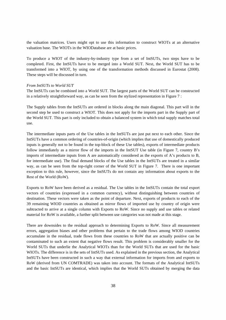
38

the valuation matrices. Users might opt to use this information to construct WIOTs at an alternative valuation base. The WIOTs in the WIODatabase are at basic prices. To produce a WIOT of the industry-by-industry type from a set of IntSUTs, two steps have to be completed. First, the IntSUTs have to be merged into a World SUT. Next, the World SUT has to be transformed into a WIOT, by using one of the transformation methods discussed in Eurostat (2008). These steps will be discussed in turn. From IntSUTs to World SUT The IntSUTs can be combined into a World SUT. The largest parts of the World SUT can be constructed in a relatively straightforward way, as can be seen from the stylized representation in Figure 7 : The Supply tables from the IntSUTs are ordered in blocks along the main diagonal. This part will in the second step be used to construct a WIOT. This does not apply for the imports part in the Supply part of the World SUT. This part is only included to obtain a balanced system in which total supply matches total use. The intermediate inputs parts of the Use tables in the IntSUTs are just put next to each other. Since the IntSUTs have a common ordering of countries-of-origin (which implies that use of domestically produced inputs is generally not to be found in the top-block of these Use tables), exports of intermediate products follow immediately as a mirror flow of the imports in the IntSUT Use table (in Figure 7, country B’s imports of intermediate inputs from A are automatically considered as the exports of A’s products to B, for intermediate use). The final demand blocks of the Use tables in the IntSUTs are treated in a similar way, as can be seen from the top-right corner of the World SUT in Figure 7. There is one important exception to this rule, however, since the IntSUTs do not contain any information about exports to the Rest of the World (RoW). Exports to RoW have been derived as a residual. The Use tables in the IntSUTs contain the total export vectors of countries (expressed in a common currency), without distinguishing between countries of destination. These vectors were taken as the point of departure. Next, exports of products to each of the 39 remaining WIOD countries as obtained as mirror flows of imported use by country of origin were subtracted to arrive at a single column with Exports to RoW. Since no supply and use tables or related material for RoW is available, a further split between use categories was not made at this stage. There are downsides to the residual approach to determining Exports to RoW. Since all measurement errors, aggregation biases and other problems that pertain to the trade flows among WIOD countries accumulate in the residual, trade flows from these countries to RoW that are actually positive can be contaminated to such an extent that negative flows result. This problem is considerably smaller for the World SUTs that underlie the Analytical WIOTs than for the World SUTs that are used for the basic WIOTs. The difference is in the sets of IntSUTs used. As explained in the previous section, the Analytical IntSUTs have been constructed in such a way that external information for imports from and exports to RoW (derived from UN COMTRADE) was taken into account. The formats of the Analytical IntSUTs and the basic IntSUTs are identical, which implies that the World SUTs obtained by merging the data

39

from these two types of IntSUTs are also of identical dimensions. As a consequence, the same steps could be used to transform both types of World SUTs into symmetric WIOTs. From World SUT to industry-by-industry WIOT The World SUT can be considered as a detailed national SUT for the world economy. Hence, well-known transformation methods to obtain symmetric input-output tables from a SUT system could be applied. As argued above, symmetric input-output tables of the industry-by-industry type will most probably be more useful than product-by-product tables. Given the choice for WIOTs of the industry-by-industry type, two transformation methods could be considered. The difference between the two methods is in the treatment of secondary products. The Supply table in the World SUT also contains a lot of positively valued cells that do not relate to the main products of an industry (since the number of products exceeds the number of industries in WIOD, this phenomenon emerges by construction). Eurostat (2008, Chapter 11) provides a very accessible explanation of the main characteristics of both methods, to which experts often refer as “Model C” and “Model D”. Model C treats secondary products according to the fixed industry sales structure assumption. This assumption boils down to assuming that each industry has its own sales structure (for intermediate input deliveries to other industries, and to various final demand categories). This implies that it sells its secondary products to exactly the same industries and final users and in exactly the same proportions as its main products. In Model D, the fixed product sales structure assumption is the point of departure. In this case, each product has its specific sales structure. It does not matter in which industry the product has been produced and consequently, the sales structure is assumed to be identical for products that have been produced as an industry’s principal output or as a secondary product by another industry. Practitioners have developed a clear preference for Model D. This preference is based on two major disadvantages of Model C. First, and most importantly, the fixed industry sales structure is considered to be much more implausible in an empirical sense than the fixed product sales structure assumption. Secondly, application of Model C can yield input-output tables with negative entries in columns where only nonnegative values should appear (i.e., in the intermediate inputs block and in consumption), even if the original SUT does not. Some somewhat ad-hoc methods have been proposed to solve these problems, but the two drawbacks of Model C taken together have been sufficient to make Model D the clearly dominant transformation method. In WIOD, this transformation method has been applied as well. The mathematical expressions that are involved in the transformation according to Model D can be found in Eurostat (2008, p. 349). For the purposes of the construction of WIOTs from World SUTs, one step was necessary that is not required when national input-output tables are constructed. In the Use tables in the IntSUTs, information about imports (by product) from RoW is contained. To transform this product-by-industry part of the table into an industry-by-industry part, a Supply table for RoW is needed. The so-called transformation matrix, which is usually derived by dividing the elements of the Supply table by product output, was estimated by constructing a condensed Supply table for the 40 WIOD countries and dividing its cells by aggregated product output. This procedure should yield a sensible estimate of the true transformation matrix if the distribution of products over supplying industries in RoW is rather similar to that of the countries covered in WIOD.

40

The construction of World SUTs from collections of IntSUTs and the transformation of these WorldSUTs into world input-output tables was applied to the IntSUTs in previous year’s prices (pyp) as well. This yielded a time series of WIOTs in pyp that is very useful for doing intertemporal comparisons and decompositions in volumes rather than in value terms. Upon the completion of these steps, the basic WIOTs were ready. Checks were done to make sure that the WIOTs were well-balanced. The remaining imbalances (which are almost without exception very small) have been included in an additional column in the WIOTs. For many research questions, such as the computation of carbon footprints and global value chain income, exports to RoW have be attributed to use categories and a domestic intermediate inputs block for RoW is needed. Below, the additional steps required to arrive at WIOD’s Analytical WIOTs that meet these requirements will be outlined. Modelling the Rest of the World (RoW) The transformation of the World SUT based on the Analytical IntSUTs yields few negative Exports to RoW (as mentioned above). Nevertheless, remaining negatives first have to be removed, otherwise it is impossible to arrive at meaningful representations of the trade flows to use categories in RoW. To attain this, negatives in the Exports to RoW column were set to zero and positive Exports to RoW by the same industries in other countries were proportionally lowered. In few cases, the original negatives were so big that it turned out impossible to ‘distribute’ the negatives over identical industries in other countries without obtaining new negatives. In such cases, a similar procedure was followed on the basis of broader aggregates of similar industries. In order to make sure that the resulting table remained balanced and could still be reconciled with National Accounts statistics, a RAS-like procedure was applied on the trade blocks of the countries involved. Hence, without modifying the domestic deliveries, new tables without negative Exports to RoW were obtained as an intermediate product. The column with non-negative exports to RoW was split into exports for intermediate use and final demand using the average export shares to these use categories by developed economies to developing economies included in WIOD. The developing economies considered are Brazil, Russia, India, China, Indonesia, and Mexico (BRICIM). For example, the average exports of Austria’s agricultural sector to the BRICIM across intermediate use industries and final demand categories was used to split up the Austrian agricultural exports to RoW. This was done cell-wise (if the exporting country was a BRICIM country, it was excluded from the BRICIM average for these particular cells). Negative values for Exports to the RoW in a particular cell were moved to changes in inventories in the final demand imports of the RoW. The domestic deliveries in RoW have been estimated, based on data collected from the UN National Accounts. These NA data by economic activity and final demand category were summed for all countries not included in WIOD to arrive at estimates of GDP by broad sectors and final demand categories for RoW. Gross output was obtained by applying the average ratio of gross output to value added for developing economies in WIOD (BRICIM). To split the broad manufacturing sector in the UN National Accounts up into the considerably more disaggregated manufacturing industries in WIOD, the average shares by industry from the UNIDO industrial statistics for all countries not included in WIOD for the period from 1995 to 2009 were used.

41

Estimates of the domestic intermediate use block and the domestic final demand block have been obtained as weighted averages shares from the BRICIM countries. For 2006-2009, in industry 29 (machinery, nec.), the sum of imported intermediate inputs used in RoW was higher than the intermediate inputs derived from UN data. In this case, we raised gross output such that estimated intermediate inputs equaled the latter. Finally, to arrive at a balanced table, for which the column sums equal the row sums for RoW, we applied the RAS algorithm. To this end, we only RASsed the domestic block of RoW in the WIOTs, which implies that exports from RoW remained unchanged. The initial values fed into the algorithm were the input coefficients from the BRICIM countries, whereas the row and column totals were given by the externally provided data based on the UN national accounts and UNIDO industrial statistics. The WIOD database also contains Analytical WIOTs in previous year’s prices (pyp). A problem specifically with respect to these tables is the fact that industry output deflators for RoW-countries are not systematically available, as a consequence of which it was impossible to use deflation procedures as applied in the construction of the IntSUTs in pyp for WIOD countries to RoW. Since demand for Analytical WIOTs in pyp is most probably high (in particular for environmental applications), all cells in the RoW blocks have been deflated by the US GDP deflators. This approximation would be close to what would be obtained if proper deflators would have been available if the exchange rates between the RoW currencies and the US dollar would be completely flexible, and the law of one price would hold. Both conditions are clearly not met in reality, but it is the best that can be attained given data availability. The steps described above led to the final output of the WIOD project, the time series of Analytical WIOTs in current prices and in previous year’s prices. Additional Input-Output Tables The WIOD database provides some additional sets of input-output tables that have been derived directly from the Analytical WIOTs, or have been constructed in a way that is fully consistent with the derivation of the basic WIOTs. First, country detail has been removed from WIOTs to arrive at world input-output tables for which the world has been split up in a limited number of (supranational) regions. These WIOT_Regs can be used for studies into the effects of changes in trade patterns among regions, without having to load the sizable and memory-intensive full WIOTs. The regions that have been defined are contained in Table 5.1. The database also contains sets of harmonized National Input-Output Tables (NIOTs) for all WIOD countries. These tables only contain information about domestic production and final demand structures, plus imports by supplying industry aggregated over all WIOD countries plus RoW. The advantage of these tables is that these are small and easy-to-use, while they have been derived in a consistent way from National Accounts data, Supply and Use Tables and data on international trade. Domestic production structures can be compared both over time and across countries. These tables might be particularly useful to illustrate proposals for new additions to the toolbox that input-output researchers have at their disposal, and might also be appropriate material for courses in input-output methods.

42

The construction of both the WIOT_Regs and the NIOTs requires a choice among two alternatives regarding the stage of the production process at which geographical aggregation should be implemented. Most commonly, aggregation is done on the basis of industry-by-industry input-output tables. The rows and columns corresponding to identical industries and final demand categories in countries that should be aggregated into one region (RoW in the case of NIOTs) are added up, which leads to tables that are fully compatible with the original, detailed input-output tables. A disadvantage of this approach is that the regionalized tables cannot be linked directly to the IntSUTs. This approach, in which the aggregation procedure is applied in the very last stage of the production process, has been followed to arrive at the Analytical WIOT_Regs and the Analytical NIOTs. Table 5.1: Regional Aggregation in WIOT_Regs* Euro-zone Non-Euro EU NAFTA China East Asia BRIIAT Austria Bulgaria Canada China Japan Australia Belgium Czech Rep. Mexico Korea Brazil Cyprus Denmark USA Taiwan India Estonia Hungary Indonesia Finland Latvia Russia France Lithuania Turkey Germany Poland Greece Romania Ireland Sweden Italy UK Luxembourg Malta Netherlands Portugal Slovakia Slovenia Spain * The Analytical WIOT_Regs also contain a full description of RoW’s production and final demand structures. Given the philosophy behind the WIOD project to construct input-output tables from Supply and Use Tables with a product dimension that can be linked well to international data on bilateral trade, an alternative approach is to construct an aggregated World SUT first (by summing over countries for corresponding industry and final demand columns and corresponding product rows). Such a regionalized World SUT can then be transformed into an input-output table of smaller dimensions than the detailed WIOTs by applying Eurostat’s Model D as outlined above. In this approach, aggregation is done at an earlier stage. There is no one-to-one aggregation scheme available between the detailed WIOTs and the regionalized input-output tables anymore, which is a downside of this approach. An advantage, however,

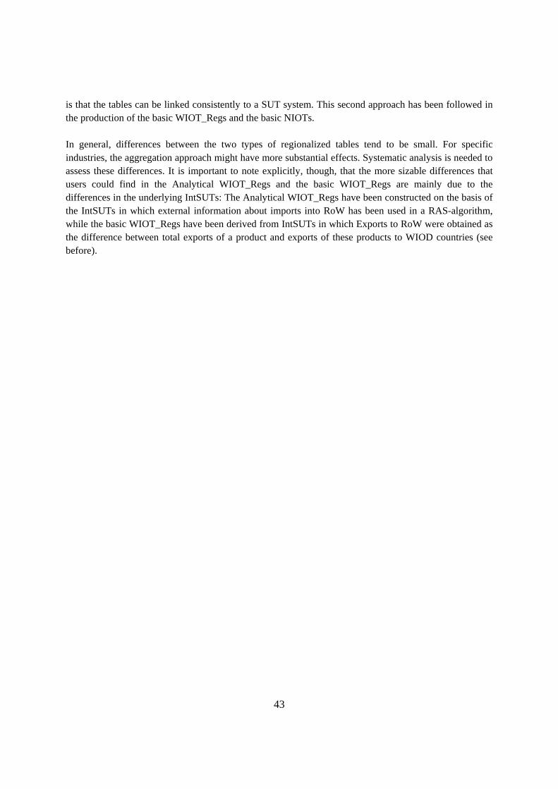
43

is that the tables can be linked consistently to a SUT system. This second approach has been followed in the production of the basic WIOT_Regs and the basic NIOTs. In general, differences between the two types of regionalized tables tend to be small. For specific industries, the aggregation approach might have more substantial effects. Systematic analysis is needed to assess these differences. It is important to note explicitly, though, that the more sizable differences that users could find in the Analytical WIOT_Regs and the basic WIOT_Regs are mainly due to the differences in the underlying IntSUTs: The Analytical WIOT_Regs have been constructed on the basis of the IntSUTs in which external information about imports into RoW has been used in a RAS-algorithm, while the basic WIOT_Regs have been derived from IntSUTs in which Exports to RoW were obtained as the difference between total exports of a product and exports of these products to WIOD countries (see before).

44

6. Environmental Accounts (EAs): Sources and Methods

6.1 Overview

At the core of the WIOD database stand the economic linkages between industries in the countries covered, portrayed by a set of harmonized supply and use tables (SUTs), alongside with data on international trade in goods and services, and integrated into sets of inter-country input-output tables. In order to expand the analytical potential of the dataset to wider range of research themes, a set of environmental satellite accounts were also developed for the WIOD project with the same time scope (1995-2009), country coverage (EU-27 Member States, 13 non-EU countries and remaining regions aggregated into a single ‘rest of the world’ region) and sector/product breakdown (35 industries plus households, 59 product groups). Other projects such as GTAP (REF #) or EXIOPOL (REF #) provide environmental data linked to an input-output (IO) framework, but to our knowledge, the WIOD environmental accounts are the first ever attempt for a publicly available full worldwide time series of a large number of environmental indicators at a reasonable sector/product breakdown.

The WIOD environmental satellites consist of energy and air emission accounts as core indicators and include also materials extraction, land use and water use as additional indicators. Core indicators (energy use and air emissions) mean they have received enhanced attention, which is justified by a number of factors. Firstly, the use of energy is usually treated as a factor of production in Economy-Energy-Environment (E3) models (such as those used in the WIOD project), and this warrants the definition of detailed links between expenditure for energy inputs and those energy inputs in physical terms. Secondly, due to the long standing existence of reporting obligations (such as in the framework of IEA16 and UNFCCC17), these themes enjoy a relatively fortunate situation in terms of data availability. Thirdly, because analyses related to the emission of greenhouse gases (such as in climate change mitigation scenarios) do not need to take into account local aspects in the same fashion that is necessary when dealing for instance with emission to water (where the adequate geographical dimension would likely be the river basin rather than the country), and this enables meso-scale models to claim full policy relevance.

In more details, the data covered by the energy accounts include energy flows (in TJ) in terms of gross

energy use and emission relevant energy use by WIOD sector and energy commodity (see Error! Reference source not found. and, and

Annex 1 for the detailed list of sectors and commodities, respectively). Once priced and aggregated, the gross energy use is directly related to expenditures for energy inputs as from the use tables and the production functions used in models. On the other hand, the emission relevant energy use, derived from the gross energy use but excluding the non-energy use (e.g. asphalt for road building) and the input for transformation (e.g. crude oil transformed into refined products) of energy commodities, is the direct link between energy use and energy-related emissions.

The air emission accounts include two sets of data: CO2 emissions (in 1000 tonnes) by sector and energy commodity (non-energy emissions are also reported) and other air pollutant emissions (in tonnes) by

                                                            16 The International Energy Agency, founded in response to the 1973-74 oil crisis, collects as a core mission authoritative and unbiased worldwide energy statistics. Data are available at: http://www.iea.org/stats/index.asp 17 The United Nations Framework Convention on Climate Change (1994), signed by 193 countries, sets an overall framework for intergovernmental efforts to tackle climate change. Data are reported to UN and are available at: http://unfccc.int/2860.php

45

sector, including N2O, CH4, NOX, SOX, NH3, NMVOC and CO. Detailed CO2 data (as opposed to providing only aggregate CO2 emissions per sector) are important to be able to simulate the environmental impact of energy mix changes (e.g. substitution of gas for coal in the power sector). Note that for the non-CO2 emissions, detailed data (by energy commodity) were either irrelevant (some emissions, such as methane are chiefly related to biomass fermentation or the use of refrigerators, not to the use of energy) or simply not feasible within the boundaries and resources of WIOD18.

For the additional indicators, the materials extraction accounts cover used materials and unused extraction (in 1000 tonnes) by extraction sector and type of materials. The used materials represent the amount of extracted resources, which enters the economic system for further processing or direct consumption; whereas the unused extraction refers to materials that never enter the economic system and thus can be described as physical market externalities (e.g. wood harvesting losses from biomass extraction). Land use accounts include the agriculture and forestry use of land (in 1000 hectares) by land type. Note that land use by other sectors (chiefly built areas) could not be included due to data gaps. Lastly, water use accounts include water use (in 1000 cubic meters) by sector and water type. A full list of materials, land and water types are included in Annex 2.

The WIOD environmental satellites may serve, for instance in the case of air emissions, to derive different environmental impact categories for analysing environmental themes of international relevance and of utmost importance. This concerns, in particular, global warming, acidification, and tropospheric ozone formation for which all the data needed to compute the potential impact19 are available in the WIOD database. In general, the environmental satellites were defined such as to cover the broadest range of environmental themes as reasonably achievable while maintaining data quality. To that respect, other environmental themes, such as waste generation and emission of pollutants to soil and water are not covered in WIOD due to severe data gaps.

The following sections depict the conceptual framework of the WIOD environmental satellites, detail the data used for elaborating the database and give an overview of the methodology implemented to derive the environmental accounts. The presentation here intends to be concise and to raise only the main points. Please refer to WIOD (2012) for full detailed information on the construction of the environmental accounts.

6.2 Conceptual framework

In brief words, environmental satellites are environmental variables of relevance for analysis, expressed mainly in physical units, which are juxtaposed to the monetary SUT framework. Figure 6.1 shows a typical arrangement for the satellites.

                                                            18 The case of CO2 is in this respect easier because CO2 combustion emissions are strictly determined by the carbon content of the fuel, which is actually fairly constant across countries and years being determined by variations in fuel quality. Adding CO2 process-based (non-energy) emissions then allows building the full emission matrix. The estimation of other pollutant emissions, conversely, requires (much) additional specific information regarding fuel quality, combustion technologies and abatement technologies. For instance, SOx emissions depend on the Sulphur content of the fuel and on the desulphurisation technology; NOx emissions depend on combustion technology (flame temperature, air-fuel ratio) and abatement techniques; etc. 19 Note that some secondary air pollutants usually considered when computing the global warming potential (e.g. SF6, CFCs and HFCs) are not covered in WIOD due to severe data gaps for allocating the emissions to specific industries. However, these secondary pollutants play a minor role in the global warming results.

46

Figure 6.1. Environmental satellites in a SUT framework (Moll et al., 2008)

For a given country and year, V represents in Figure 6.1 the make table (transpose of the domestic supply table) and I the vector of imported products from the supply side, while from the use side, U denotes the inter-industry part of the use table (intermediate consumption), Y the final demand matrix (consumption by private households and government, gross fixed capital formation and exports) and w the gross value added vector by industry (comprising several factor inputs such as wages, depreciation and surplus). Row wise, vector q shows total use of products by industries and final demand while vector x is the output by industry (domestic production). Column wise, vector qT is the transposed total supply of products (domestically produced or imported) while transposed vector xT is total input by industry (intermediate products and value-added). The SUT framework as illustrated in Figure 6.1 is balanced and expressed in monetary units, with industry input equalling industry output (x, xT) and product supply equalling product use (q, qT). These identities are an important prerequisite for the mathematical Leontief-type models.

A simple and convenient means of adding the environmental variables (extensions), while keeping the system balanced, is to juxtapose them as an extension of the SUT, using so-called satellite accounts. Satellite accounts are thus external vectors, juxtaposed using the same product and industry breakdown as the SUT they accompany. Figure 6.1 illustrates the treatment of an environmental variable (e.g. CO2 emissions) in the form of vector rT. The juxtaposed vector comprises two parts: rx related to industries and representing direct environmental factor inputs by industry, and rY represents factor inputs associated to the components of final demand. This framework, sometimes called NAMEA (National Accounting Matrices including Environmental Accounts), accepts as many extensions as environmental variables of interest one needs to add. Since all environmental account data published by National Statistics Institutes (NSIs) follow the publication of compatible national accounts, the terms NAMEA and environmental accounts are frequently used as synonyms, in particular NAMEA-energy for energy accounts and NAMEA-air for air emission accounts.

The presented framework is entirely based on the residence principle and directly suitable for analysis using e.g. IO models of Leontief type (with industry technology or commodity technology assumptions). In addition, compared to an environmental extended IO system based on symmetric tables, the EE-SUT (Environmentally Extended SUT) offers the flexibility of recording the supply and use of residuals either

I

products industries

pr

od

uc

ts

in

du

st

ri

es

U

V

r xT

q T

Y q

x

x T

w

r yTextensions

47

by industries or by products; this distinction will be useful in the definition of the environmental satellite accounts related to the production of goods and services and to their use.

The total environmental load related to the consumption of products is in fact customarily broken down in three main components: production phase (including raw material production, manufacture of the product, and distribution), use phase, and post-consumer phase (waste management). Not that the post-consumer phase is related to waste accounts which are not covered in WIOD. Having made the distinction between environmental loads of the production phase (only relevant for industries) and of the use phase (relevant both for industries and final consumers), we finally remark that not all the final demand elements of the environmental satellite accounts need to be filled: final consumption by households has associated environmental account entries; final consumption by government and not-for-profit organisations does not due to accounting conventions20; and other final uses do not have associated emissions either: investments do not because they are not clearly associated to flows responsible for emissions in the calendar year while exports do not because the use of those goods – and the emissions associated – in accordance to the overarching residence principle shall be booked to the importing country.

6.3 Data used

To compile the environmental accounts, various sources of information were used. They are reviewed below. The overarching principle of the data collection effort was to include, to the extent possible, all known and accessible official data published by NSIs in a format similar to the target WIOD format, i.e. in NAMEA-like format. However, despite the publication of international guidelines (SEEA, 2003), there is currently no international reporting for environmental accounts in general and NAMEA-like data are scarce. Whenever NAMEA data were not available, other statistics covering the same variables were collected to be converted to the NAMEA standard by means of the estimation procedures described in the methodology section and with the help of the required auxiliary data.

First of all, a general source of information for the environmental extensions is the other parts of the WIOD database itself, including the SUTs and socio-economic accounts, which guaranties the consistency of the whole WIOD database.

Regarding energy specific data, according to a survey conducted by the UNSD (2009), some 30-35 countries worldwide have developed, for at least one year, energy accounts based on a national accounting framework though at different industry/energy commodity breakdown levels. However, only a handful of countries have published and made available the results. The following energy accounts from NSIs were used in WIOD: Austria, Denmark, Germany, The Netherlands, Australia and Canada. As a result, the main source of information for WIOD energy accounts is the energy balances from IEA (2011a), available for all WIOD countries and years and which consist of energy inventories using territorial principle and technology- and/or process-based classifications which are in certain cases difficult to link to economic activities. The “Energy Statistics Manual” jointly published by IEA, Eurostat and OECD (2004) is the main reference for the concepts and classifications of energy balances and statistics. To circumvent the major difficulties to derive energy accounts from energy balances

                                                            20 Government consumption records expenditure for services provided (CPA75 for public administration services, CPA80 for education, CPA85 for health, etc.), while the use of inputs such as fuels is not in the government consumption but in the input structure of the sectors NACE75 (sector L), NACE80 (sector M), NACE85 (sector N), etc.

48

(differences in classification, terminology, source and boundary principle), specific sources of information were gathered. This encompass energy prices from IEA (2011b), transport data including aviation and marine bunkering from EXIOPOL (REF#), car fleet from ODYSSEE (2011) and average fuel efficiency (JRC/CONCAWE/EUCAR, 2008), and tourism data including tourism terms of trade statistics from OECD-Eurostat (REF#).

For air emission data, the main source of information for EU Member States is the full EU27 NAMEA-air dataset from Eurostat (2012a). All the WIOD air pollutants are covered and the time series ranges from 1995 to 2008. For non-EU countries, only international air emission inventories could be used. These include the inventory from the UNFCCC (2011) which covers all WIOD years and pollutants but ammonia for WIOD countries except: Brazil, China, South Korea, India, Indonesia, Mexico and Taiwan; and the inventory from the Emission Database for Global Atmospheric Research (EDGAR, 2011) which covers all WIOD pollutants and countries until 2008. In addition, information on CO2 emission factors were gathered from the 2006 IPCC Guidelines for National Greenhouse Gas Inventories (IPCC, 2006) as well as from UNFCCC (2011) emission reporting where country-specific emission factors are also reported (in that case the latter information supersedes the 2006 IPPC guidelines).

For the other environmental extensions, the sources for materials extraction include the database of material flows from SERI/Wuppertal Institute (2011) and the Material Flow Accounts (MFAs) from Eurostat (2012a), which both are based on a series of methodological guidebooks for economy-wide MFA (Eurostat, 2001 and 2009). SERI/Wuppertal Institute database covers all WIOD materials and countries until 2008 while Eurostat database covers EU27 countries and Turkey for used materials only ranging from 2000 to 2007 (some countries have also provided data 1995-1999 and 2008-2009). For agricultural and forestry land use, the main source used was FAOSTAT, the statistical system of the Food and Agriculture Organisation of the United Nations (FAO, 2012), covering all WIOD land use21 and countries but Taiwan until 2008. For water accounts, the main data source is the series of studies on the calculations of water footprints conducted by Mekonnen and Hoekstra (2010a,b, and 2011a,b). Additional information used for the other environmental extensions includes FAOSTAT agricultural production (FAO, 2012), data on water use from EXIOPOL (REF#), data on hydropower from IEA (2011a) and population data from UN (2011).

6.4 Methodology

The environmental accounts in WIOD follow the principles laid down in SEEA (2003) and then can be called as NAMEA-energy, NAMEA-air, NAMEA-materials, NAMEA-land and NAMEA-water.

For NAMEA-energy, two main concepts in a balanced accounting framework can be used: net vs. gross energy concept. In the case of gross energy supply and use, the following equation holds:

                                                            21 Note that forestry land use is not covered as such.

49

Gross supply: Domestic production + Imports + Inventory changes

=

Gross use: Intermediate consumption + Final uses + Exports

While in the case of net energy supply and use, we have:

Net supply: Direct extraction + Imports + Inventory changes

=

Net use: Final uses + Losses due to conversion + Exports

WIOD energy accounts are based on the gross energy use concept which means that one has some double counting regarding the total energy metabolism of an economy (e.g. records of crude oil as input to refineries and refined products as input to all sectors, or natural gas as input to power sector and electricity consumption by all sectors, etc.). However, this gross energy concept is fully consistent with the input records in the use tables and all the information on the country energy mix is kept, which makes the environmental accounts with such concept more suitable for modelling applications (e.g. fuel substitution). Note that the emission relevant energy use is also estimated in WIOD to compute later the emissions to avoid any double counting.

Energy accounts are compiled using IEA extended energy balances as a starting point, achieving the specification of energy accounts using additional information to bridge between territory and residence principles and to allocate IEA accounts to the target classification and accounting concepts. The easy part of the work is when some of the energy balance items can be directly linked to some WIOD economic activities (e.g. agriculture and fisheries, paper production inputs, etc.). The main issues in energy account construction include the mismatch between sector classifications of IEA balances and WIOD, the discordant conceptual definition of some sectors, the different boundary principles, the inconsistencies between IEA data and WIOD SUTs, and the alignment of WIOD accounts with official NAMEA energy. In case of sector mismatch (e.g. textiles, miscellaneous manufacturing, services), the input of energy commodities (CPA 02, 10, 11, 23, 40 and 90) in monetary terms from the use table is used as the splitting key based on the two following assumptions: the NACE sectors that are below an aggregate IEA heading (e.g. services) a) pay the same price per energy unit, and b) consume energy products below an aggregate CPA heading (e.g. refined products) with identical shares given by the energy product shares of the corresponding IEA extended energy balance account.

Regarding discordant sector definition (e.g. heat and electricity autoproduction, road transport), some reassignments have to be made based on WIOD SUT information and combined with additional information and assumptions. For instance, the electricity and heat autoproduction (produced by non-power sectors) by specialised fuels has been directly assigned to specific sectors (e.g. autoproduction by

50

waste to the waste management sector), whereas for the fuels of general use (e.g. natural gas), CAP 40 supply is used as a splitting key assuming that the share of power generation not captured in the supply table is equal for all industries that autoproduce electricity22. For road transport, household and road transport sectors fuel consumption was computed with combining monetary expenditure from use tables and composite fuel price23 based on IEA energy prices, passenger car fleet and car motor efficiencies; whereas the residual amount of fuels, corrected for the residence principle (see after), is assigned among all other sectors using the number of employees as the splitting key.

The boundary difference (territorial vs. residence principle) mainly affects transportation. For road transport, household and road transport sectors fuel consumption is already conformant with residence principle given that the estimation is based on SUTs information. For the other sectors (residual), a correction with the aid of tourism terms of trade statistics (Eurostat-OECD) was applied. For air transport, the energy input flows (chiefly jet fuel) are based on the expenditure for commodity CPA 23 by the aviation sector priced with IEA information, which provide data according to residence principle. For maritime transport, the same procedure produced poor results, so the following alternative was applied: one point estimate in time (based on the estimates from the EXIOPOL project) was used to compute the ratio between fuel use by national carriers and bunker fuel deliveries in the country and this was projected along the time series with the supply of maritime transport services by the maritime transport sector in constant prices with keeping that ratio as constant (assuming fully constant energy use per output, which may be acceptable in maritime transport where room for innovation is limited).

Note that inconsistencies between IEA data and WIOD SUTs were corrected on case by case basis while the alignment with official NAMEA energy was ensured with calibrating the WIOD time series at sector and energy commodity levels.

In the case of NAMEA-air, they may rely on two different concepts: energy-first vs. inventory-first approach (Eurostat, 2009). In energy-first approach, the estimation procedure starts from energy data re-arranged into energy accounts and applies emission factors (with taking into account non-energy related emissions) to derive air emissions. In inventory-first approach, it starts from national emission inventories, adjusts for residence principle and allocates the process-oriented emissions to economic activities to derive air emissions. For WIOD air emission accounts, the following strategy was implemented: NAMEA-air like data were given priority when available; energy-first approach was used when most emissions linked to fuel combustion (CO2, NOx, SOx, NMVOC and CO); and inventory-first approach was applied when most emissions are not linked to energy use (N2O, CH4 and NH3).

In the case of energy-first approach, the main issues concern non-energy related CO2 and non-CO2 sectoral emission factors. Non-energy related CO2 emissions are not available for non-reporting UNFCCC countries and were estimated based on average ratio energy vs. non-energy drawn from know countries. Non-CO2 emission sectoral factors which are not available for non-EU countries were estimated with calibrated coefficients based on EU sectoral emission factors. In the case of inventory-first

                                                            22 Note that the CAP 40 supply represents not only the sale of surplus electricity to the grid from those establishments but also the supply of electricity within the same firm, as long as the production of electricity occurs in a different establishment (belonging to the same firm) than the one consuming electricity, and as long as the statistical authority applies consistently this accounting convention; in practice it is common, however, that empirical hurdles cause part of these flows to be unrecorded. In order to circumvent the statistical volatility of the non diagonal elements regarding electricity supply, the supply tables were averaged along the whole WIOD time series. 23 For road transport sectors, the composite fuel price is simply equal to diesel price as it is assumed that these sectors only own diesel transport equipment (assumption by and large verified in the NAMEA-energy data available from NSIs).

51

approach, the main concerns are the mismatch between inventory and SNA classifications and the different boundary principles. For the classification mismatch, the same strategy as for energy accounts was applied (WIOD use table information combined with the same kind of assumptions). For residence principle correction, some scaling factors were applied.

The main methodological aspects of the construction of the additional indicators are related to the sectoral allocation and to the estimation of data gaps. In the case of material extraction, the allocation of materials to sectors is straightforward: biomass extraction is allocated to agriculture (sector AtB) while the extraction of fossil fuels and minerals corresponds to mining (sector C). The Eurostat database is the main source for the material extraction used in the EU27 countries, while the SERI/Wuppertal data set constitutes the base for the used and unused in the non EU27 countries, and for the unused in the EU27. When data is missed for a EU27 country the estimations has been conducted using the SERI/Wuppertal database. When data for 2009 is not available, it has been estimated on the basis of the gross output at constant prices.

Agricultural area and forest area in the land accounts are allocated to agriculture sector. Forest area includes an estimation of the area actually used for productive purposes, as suggested by Lugschitz, et al. (2011). These figures have been extrapolated from the forest area used for production purposes reported by FAO (2006).

Water use in the agricultural sector has been estimated using crop and livestock water intensities from Mekonnen and Hoekstra (2010a,b) and data on crop production and livestock from FAOSTAT. The use24 of water of the electricity sector (sector E) for hydropower generation has been calculated using the world average water use per unit of electricity estimated by Mekonnen and Hoekstra (2011b)25 and the hydropower generation from the IEA. The use of water in the other economic sectors has been calculated using the total water use in industry reported by (2011a), the shares of water use by industry of EXIOPOL and the gross output at constant prices from WIOD. Finally, water use by households is estimated on the basis of the average domestic water supply from Mekonnen and Hoekstra (2011a) and population from United Nations.

Bibliography for this section

EDGAR (2011): Emissions Database for Global Atmospheric Research, v4.2 release, EDGAR project, European Commission, available at: http://edgar.jrc.ec.europa.eu/index.php

Eurostat (2009): Manual for Air Emissions Accounts. Methodologies and working papers. ISBN 978-92-79-12205-7. European Communities, Luxembourg. http://epp.eurostat.ec.europa.eu/cache/ITY_OFFPUB/KS-RA-09-004/EN/KS-RA-09-004-EN.PDF

Eurostat (2012a): Environment statistics, European Commission, available at: http://epp.eurostat.ec.europa.eu/portal/page/portal/environment/introduction

                                                            24 This water refers to the water evaporated from manmade reservoirs to produce electric energy. 25 68 m3/GJ

52

Eurostat (2012b): ESA 95 Supply, Use and Input-Output tables, European Commision, available at: http://epp.eurostat.ec.europa.eu/portal/page/portal/esa95_supply_use_input_tables/introduction

EXIOPOL (2011): A new environmental accounting framework using externality data and input-output tools for policy analysis, FP6 Research Project: 2007-2011. http://www.feem-project.net/exiopol/

FAO (2006). Global Forest Resources Assessment 2005. Progress towards sustainable forest management. FAO, Rome, 2006

FAO (2012): FAOSTAT. The statistical system of the Food and Agriculture Organisation of the United Nation, http://faostat.fao.org/

GTAP (2008): Global Trade Analysis Project. Version 7. Deaprtment of Agricultural Economics, Purdue University, US; https://www.gtap.agecon.purdue.edu/databases/default.asp

IEA (2011a): Energy balances of OECD and non-OECD countries, 2011 Edition, available at: http://www.iea.org/index.asp

IEA (2011b): Energy prices and taxes, 2011 Edition, available at: http://www.iea.org/index.asp

IEA/Eurostat/OECD (2004): Energy statistics manual. IEA/OECD Publication services, Paris, France. http://www.iea.org/textbase/nppdf/free/2004/statistics_manual.pdf

IPCC (2006): 2006 IPCC Guidelines for National Greenhouse Gas Inventories. Prepared by the National Greenhouse Gas Inventories Programme.

JRC/CONCAWE/EUCAR (2008): Well-to-wheels analysis of future automotive fuels and powertrains in the European context; Tank-to-Wheels Report, Version 3, October 2008.

Lugschitz, B., Bruckner, M., Giljum, S. (2011). Europe’s global land demand. A study on the actual land embodied in European imports and exports of agricultural and forestry products. Sustainable Europe research Institute, Vienna.

Mekonnen, M. and Hoekstra, A. (2010a): The green, blue and grey water footprint of farm animals and animal products, Value of Water Research Report Series No.48, Volume I and II. UNESCO-IHE, Delft, the Netherlands.

Mekonnen, M. and Hoekstra, A. (2010b): The green, blue and grey water footprint of crops and derived crop products. Value of Water Research Report Series No.47, Volume I and II. UNESCO-IHE, Delft, the Netherlands.

Mekonnen, M., Hoekstra, A. (2011a): National water footprint accounts: the green, blue and grey water footprint of production and consumption. Value of Water Research Report Series No.50, Volume I and II. UNESCO-IHE, Delft, the Netherlands.

Mekonnen, M., Hoekstra, A. (2011b): The water footprint of electricity from hydropower. Value of Water Research Report Series No.51. UNESCO-IHE, Delft, the Netherlands.

Moll, S., Giljum, S., Lutter, S., Acosta, J. (2008): Technical Report on Basic Conceptions for Environmental Extensions of Input-Output Framework. EXIOPOL Deliverable DIII.2.b-1 and DIII.3.b-1. Final draft 16 July 2008. http://www.feem-project.net/exiopol/

53

ODYSSEE (2011): Energy efficiency indicators in Europe, ODYSSEE MURE project, European Commission, available at: http://www.odyssee-indicators.org/

OECD (2011): Tourism Statistics http://unstats.un.org/unsd/tradeserv/tourism.htm

SEEA (2003): Handbook of National Accounting: Integrated Environmental Accounting 2003.United Nations, European Commission, International Monetary Fund, Organisation for Economic Co-operation and Development. UN, New York. http://unstats.un.org/unsd/envaccounting/seea2003.pdf

SERI (2011): Material flow database, Sustainable Europe Research Institute and Wuppertal Institute, available at: www.materialflows.net

UN (2011): State of World Population 2011; United Nations, http://www.unfpa.org/swp/

UNFCCC (2011): National inventory submissions: Common reporting format, United Nations Framework Convention on Climate Change, available at: http://unfccc.int/national_reports/annex_i_ghg_inventories/national_inventories_submissions/items/5888.php

UNSD (2009): Report on the Global Asssessment of energy accounts. UN Statistics Division, NY. February 2009. http://unstats.un.org/unsd/envAccounting/ceea/surveyEEA.asp

WIOD (2012): World Input-Output Database: Construction and Applications, FP7 Research Project, 2009-2012; www.wiod.org

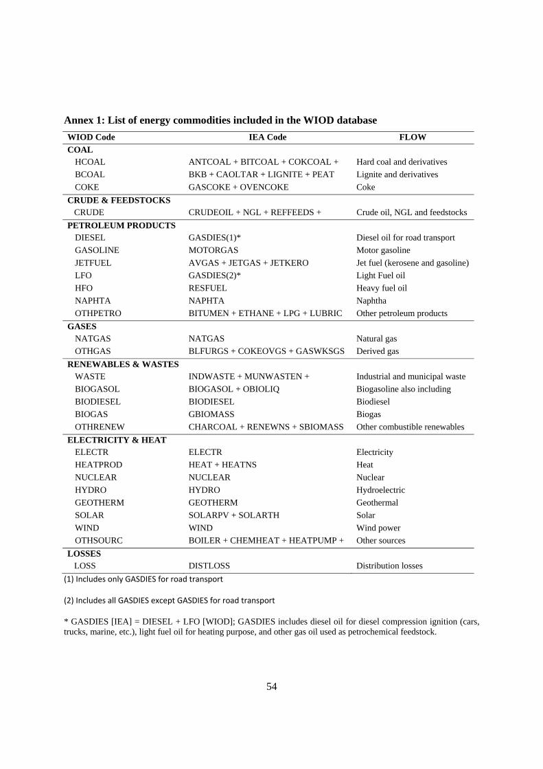
54

Annex 1: List of energy commodities included in the WIOD database

WIOD Code IEA Code FLOW

COAL HCOAL ANTCOAL + BITCOAL + COKCOAL + Hard coal and derivatives

BCOAL BKB + CAOLTAR + LIGNITE + PEAT Lignite and derivatives

COKE GASCOKE + OVENCOKE Coke

CRUDE & FEEDSTOCKS CRUDE CRUDEOIL + NGL + REFFEEDS + Crude oil, NGL and feedstocks

PETROLEUM PRODUCTS DIESEL GASDIES(1)* Diesel oil for road transport

GASOLINE MOTORGAS Motor gasoline

JETFUEL AVGAS + JETGAS + JETKERO Jet fuel (kerosene and gasoline)

LFO GASDIES(2)* Light Fuel oil

HFO RESFUEL Heavy fuel oil

NAPHTA NAPHTA Naphtha

OTHPETRO BITUMEN + ETHANE + LPG + LUBRIC Other petroleum products

GASES NATGAS NATGAS Natural gas

OTHGAS BLFURGS + COKEOVGS + GASWKSGS Derived gas

RENEWABLES & WASTES WASTE INDWASTE + MUNWASTEN + Industrial and municipal waste

BIOGASOL BIOGASOL + OBIOLIQ Biogasoline also including

BIODIESEL BIODIESEL Biodiesel

BIOGAS GBIOMASS Biogas

OTHRENEW CHARCOAL + RENEWNS + SBIOMASS Other combustible renewables

ELECTRICITY & HEAT ELECTR ELECTR Electricity

HEATPROD HEAT + HEATNS Heat

NUCLEAR NUCLEAR Nuclear

HYDRO HYDRO Hydroelectric

GEOTHERM GEOTHERM Geothermal

SOLAR SOLARPV + SOLARTH Solar

WIND WIND Wind power

OTHSOURC BOILER + CHEMHEAT + HEATPUMP + Other sources

LOSSES LOSS DISTLOSS Distribution losses

(1) Includes only GASDIES for road transport 

(2) Includes all GASDIES except GASDIES for road transport 

* GASDIES [IEA] = DIESEL + LFO [WIOD]; GASDIES includes diesel oil for diesel compression ignition (cars, trucks, marine, etc.), light fuel oil for heating purpose, and other gas oil used as petrochemical feedstock.

55

Annex 2: List of materials, land and water types covered in the WIOD database

WIOD Code FLOW

MATERIALS TYPE Biomass

Biomass_animals_Used Animal biomass (used)

Biomass_animals_Unused Animal biomass (unused)

Biomass_feed_Used Feed biomass (used)

Biomass_feed_Unused Feed biomass (unused)

Biomass_food_Used Food biomass (used)

Biomass_food_Unused Food biomass (unused)

Biomass_forestry_Used Forestry biomass (used)

Biomass_forestry_Unused Forestry biomass (unused)

Biomass_other_Used Other biomass (used)

Biomass_other_Unused Other biomass (unused)

Fossil fuels

Fossil_coal_Used Coal (used)

Fossil_coal_Unused Coal (unused)

Fossil_gas_Used Natural gas (used)

Fossil_gas_Unused Natural gas (unused)

Fossil_oil_Used Crude oil (used)

Fossil_oil_Unused Crude oil (unused)

Fossil_other_Used Other fossil fuels (used)

Fossil_other_Unused Other fossil fuels (unused)

Other materials

Minerals_construction_Used Non-metallic minerals for construction (used)

Minerals_construction_Unused Non-metallic minerals for construction (unused)

Minerals_industrial_Used Other non-metallic minerals (used)

Minerals_industrial_Unused Other non-metallic minerals (unused)

Minerals_metals_Used Metals (used)

Minerals_metals_Unused Metals (unused)

LAND TYPE Arable_area Arable land

PermanentCrops_area Permanent crops

Pastures_area Permanent meadows and pastures

Forest_area Productive forest area

WATER TYPE Water_blue Blue water

Water_green Green water

Water_gray Gray water

 

56

7. Socio-economic Accounts (SEAs): Sources and Methods

The Socio-Economic Accounts (SEAs) contain annual data (1995-2009) for 35 industries on

Industry output, value added, at current and constant price

Capital stock and investment

Wages and employment by skill type (low-, medium- and high-skilled).

The full set of variables in a SEA for each country are given in Table 1

Table 7.1 Variables in the WIOD Socio-economic Accounts (SEA)

Values Description GO Gross output by industry at current basic prices (in millions of national currency) II Intermediate inputs at current purchasers' prices (in millions of national currency) VA Gross value added at current basic prices (in millions of national currency) COMP Compensation of employees (in millions of national currency) LAB Labour compensation (in millions of national currency) CAP Capital compensation (in millions of national currency) GFCF Nominal gross fixed capital formation (in millions of national currency) EMP Number of persons engaged (thousands) EMPE Number of employees (thousands) H_EMP Total hours worked by persons engaged (millions) H_EMPE Total hours worked by employees (millions)

Prices GO_P Price levels gross output, 1995=100 II_P Price levels of intermediate inputs, 1995=100 VA_P Price levels of gross value added, 1995=100 GFCF_P Price levels of gross fixed capital formation, 1995=100

Volumes GO_QI Gross output, volume indices, 1995 = 100 II_QI Intermediate inputs, volume indices, 1995 = 100 VA_QI Gross value added, volume indices, 1995 = 100 K_GFCF Real fixed capital stock, 1995 prices

Additional variables

LABHS High-skilled labour compensation (share in total labour compensation) LABMS Medium-skilled labour compensation (share in total labour compensation) LABLS Low-skilled labour compensation (share in total labour compensation) H_HS Hours worked by high-skilled persons engaged (share in total hours) H_MS Hours worked by medium-skilled persons engaged (share in total hours) H_LS Hours worked by low-skilled persons engaged (share in total hours)

57

The sources used for Industry output, value added, at current and constant price are described in more detail in “Sources for National Supply and Use Table Input files” , Abdul Azeez Erumban, Reitze Gouma, Gaaitzen de Vries, Klaas de Vries and Marcel Timmer, April 2012. This section describes the sources and methods for estimating labour and capital input.

7.1 Wages and employment by skill types

For factor input requirements we collected country-specific data on detailed labour inputs for all 35 industries. This includes data on hours worked and compensation for three labour types (low-, medium- and high-skilled labour) and data on capital stocks and compensation. These series are not part of the core set of national accounts statistics reported by NSIs. The database builds upon the data collected in the EU KLEMS project (see www.euklems.net described in O’Mahony and Timmer 2009) by updating it and extending it to a larger set of countries. Within EU KLEMS this type of data is available for about 15 OECD countries up to the year 2007. We extend this data to include also a large set of less developed countries and update to 2009. This extensive coverage of the SEAs in WIOD makes it a unique database compared to what is currently available.

Skills in the WIOD SEAs are defined on the basis of educational attainment levels. Data on number of workers by educational attainment are available for a large set of countries (e.g. Barro and Lee, 2010), but WIOD provides an extension in two directions. First, the WIOD SEAs provide industry level data, reflecting the large heterogeneity in the skill levels used in various industries (compare e.g. agriculture and financial and business services). This has been documented in e.g. Jorgenson and Timmer (2011) for the OECD countries, and this heterogeneity is even stronger in less developed countries. Moreover, the WIOD SEAs also provide relative wages by skill type that reflect the differences in remuneration of workers with different levels of education. The wage data is made consistent with the quantity data and can be used in conjunction to analyse distributional issues such as relative income shares.

Data on wages and employment by skill types are not part of the core set of national accounts statistics reported by NSIs; at best only total hours worked and wages by industry are available from the National Accounts. Additional material has been collected from employment and labour force statistics. For each country covered, a choice was made of the best statistical source for consistent wage and employment data at the industry level. In most countries this was the labour force survey (LFS). In most cases this needed to be combined with an earnings surveys as information wages are often not included in the LFS. In other instances, an establishment survey, or social-security database was used. Care has been taken to arrive at series which are time consistent, as most employment surveys are not designed to track developments over time, and breaks in methodology or coverage frequently occur. For most OECD countries labour data was taken from the EU KLEMS database (www.euklems.org, described in O’Mahony and Timmer 2009), revised and updated. For countries not in EU KLEMS new sources have been used.

Labour compensation of self-employed is not registered in the National Accounts, which as emphasised by Krueger (1999) leads to an understatement of labour’s share. This is particularly important for less advanced economies that typically feature a large share of self-employed workers in industries like agriculture, trade, business and personal services. We make an imputation. For advanced countries, we

58

assume that the compensation per hour of self-employed is equal to the compensation per hour of employees. For emerging countries this assumption is not plausible as a large part of informal workers earns much less than the average wage of low-skilled workers. Instead, we used additional information which differs by country. This is described in the country notes below.

In WIOD three skill types of labour are being distinguished. Skill type is defined on the basis of the level of educational attainment of the worker. Educational systems and attainment levels are not always comparable across countries in a straightforward manner. We use the 1997 International Standard Classification of Education (ISCED) classification to define low, medium and high skilled labour. The definition of skills is given in Table 1. For more information on ISCED, see http://www.uis.unesco.org/Education/Pages/international-standard-classification-of-education.aspx

Table 7.2 Definition of skills in WIOD SEA

WIOD skill-type

1997 ISCED

level

1997 ISCED level description

Low 1 Primary education or first stage of basic education Low 2 Lower secondary or second stage of basic education Medium 3 (Upper) secondary education Medium 4 Post-secondary non-tertiary education High 5 First stage of tertiary education High 6 Second stage of tertiary education

Data has been collected for both the number of workers, and their wages. If available the data refers to all workers including self-employed and family workers, but mostly they refer to employees only. This is indicated for each country in the country source notes below. Numbers refer to numbers of workers and do not adjust for differences in hours worked. The latter is preferable, but based on the available evidence there is no clear relationship between hours worked and skill-level.

In principle, data is constructed for the period from 1995 to 2009. Annual availability of data differs across countries. Also, data on wages is scarcer than for number of workers and more imputations have to be made. For each country we have at least one observation of wages in this period, to ensure that country-specific skill-premia are reflected in the data, and match with the definition for quantities. For most countries we have at least three observations across the period to reflect the changes in skill premia that take place over time.

The level of industry detail also varies across countries and depends crucially on the sample sizes of the surveys on which our estimates are based. Quantity data by skill type is available for at least 14 industries in all countries, up to 35 in some (e.g. India and Mexico). In order to derive shares for all 35 WIOD industries we assume that the skill distribution of workers in sub-industries is similar as the shares for more aggregate industries.

59

Relative wage data is scarcer. Sometimes it is available at a more aggregate level than data for quantities. e.g. for China only for 3 broad sectors. We assume that relative wages of both high-skilled and medium-skilled workers relative to low-skilled in sub-industries is the same as in the more aggregate industry. As relative wages will differ much less across industries than quantities this assumption can more easily be made at higher levels of aggregation. For example, while in say China the relative number of high to low-skilled workers is much higher in chemicals than in textile manufacturing, the relative wages of high-to-low skilled workers in both industries will be closer together. Also, relative wage data is not always available on an annual basis. In those cases we interpolate relative wages for years in-between. As relative wages develop only slowly, this assumption is relatively harmless.

For the European countries labour shares and labour compensation shares are estimated based on shares from the EUROSTAT Labour Force Surveys (LFS). The LFS provides data on the fraction of High, Medium and Low skilled labour in total workers (and sometimes hours worked) and labour compensation for 14 separate sectors of the economy, which sum to total economy. The shares of these 14 sectors are used as data for the more detailed underlying industries. LFS provides data up to 2009 for all countries, however, the starting year differs from country to country. Relative wage data is from the EU Structural Earnings Survey (SES) and EU Survey on Income and Living Standards (SILC). In order to complement the data such that it includes the skill shares from 1995 up to 2009, the LFS data needs to be extrapolated backwards to 1995. This is done by using the skill-shares from the March 2008 release of the EU KLEMS database insofar available. For non-EU countries various country-specific data sources are used. Details can be found in the section on country sources and methods.

7.2 Investment and capital stocks

The capital data in the WIOD SEAs include investment and capital stocks at current and constant prices. While this type of data is available for the total economy (see e.g. Total economy Database The Conference Board) there is no large-scale database that provides industry level detail. Heterogeneity of capital and investment flows across industries is even bigger than for labour, and taking account of this is crucial in any analysis of the role of capital in structural change and economic growth.

The WIOD SEAs contain investment and capital stock series by industry at both current and constant prices. The series cover all fixed assets as defined in the SNA 1993. Data on capital stocks is only available up to 2007 unless otherwise indicated. The EU KLEMS database provides investment, stocks and capital services data cross-classified by both industry and eight asset types. For those countries for which EU KLEMS data was available we took the investment and stock estimates directly. These are given in the so-called capital input files on the EU KLEMS website and the files can be used when more detailed information on stocks or services is needed.26

This type of data is available for a limited set of OECD countries in the EU KLEMS database, but not for the majority of the 40 WIOD countries. For the other countries, capital stocks have been constructed on

                                                            26 For the European countries for which EU KLEMS capital stocks data is used the Textiles, Textile, Leather and Footwear sector (NACE Rev.1.1 sector 17t19) has been split into Textiles and Textile (industry 17t18) and Leather and Footwear (industry 19) separately using Value Added shares. The same was done to split the EU KLEMS aggregate sector Transport and Storage (industry 60t63) into the transport of water, land and air and other transport activities separately.

60

the basis of the Perpetual Inventory Method (PIM) in which the capital stock (K) in year t is estimated as the sum of the depreciated capital stock in year t-1 plus real investment (I) in year t:

Kt = (1-d)Kt-1 +It

with d the depreciation rate. The depreciation rates are taken to be geometric and industry-specific and given in Appendix Table 1. They take into account the differences in the composition of capital assets in various industries and vary from less than 4% in e.g. Education and Public Administration to more than 10% in financial and business services. This takes into account the larger share of long-lived assets as buildings and structures in the former, and the larger share of short-lived assets like ICT-equipment and software in the latter. The industry-specific rates are based on weighted asset-specific depreciation rates used in EU KLEMS. The 8 asset types are weighted by the asset distribution within industries for Spain and averaged over the period 1995-2006. The industry-specific rates are assumed to be the same for all countries due to lack of sufficient country-specific information.

For many countries long time-series of investments are available and there is no need to have information on an initial stock estimate. In cases where investment series were too short, and did not start at least 20 years prior to 1995, an initial capital stock for 1995 had to be estimated. Two alternatives were used: the ICVAR and Harberger method.

ICVAR method. For countries were no investment data before 1995 was available, the ICVAR method was used (see e.g. Timmer 1999 for an application). In the ICVAR method, industry specific ratios of value added to capital stocks were used of a country at a similar stage of development (often Spain). These industry-specific ratios (averaged over 5 years to smooth out business cycle fluctuations) were applied to the 1995 value added to derive the 1995 capital stock. For years after 1995 the PIM method was used based on this 1995 estimate.

Harberger method. For countries for which investment series were available for a number of years before 1995, but less than 20, an initial capital stock for the year in which investment series start is estimated using the Harberger method (Harberger, 1978; Easterly and Levine, 2001). The Harberger method can be written as:

K0 = (i/(g+d)) * GO,

Where K0 is the initial capital stock in constant 1995 prices, GO is gross output by industry in constant 1995 prices, i is the investment rate (GFCF in 1995 prices divided by GO in 1995 prices by industry), g is the average growth rate of output, and d is the total depreciation rate by industry. For most countries, gross output series extend back to 1970 and we used the average growth rate for the period 1970-1994 as an estimate for g. For other countries were only gross output series from 1995 onwards. Capital stocks are estimated at the level of 35 industries unless otherwise indicated.

More information, and country specific sources used can be found in Erumban, Gouma, de Vries, de Vries and Timmer (2012) WIOD Socio-Economic Accounts (SEA): Sources and Methods

 

61

References:

Backer, K. De & Norihiko Yamano (2007). "The Measurement of Globalisation using International

Imput-Outpout Tables," OECD STI Working Papers 2007/8, OECD, Directorate for Science, Technology and Industry.

Eurostat (2008) Eurostat Manual of Supply, Use and Input-Output Tables (Luxembourg, Eurostat). Erumban, A.A., F.R. Gouma, G. de Vries, K. de Vries and M.P. Timmer (2012), WIOD Socio-Economic

Accounts (SEA): Sources and Methods, background document downloadable at www.wiod.org.

Erumban, A.A., F.R. Gouma, G. de Vries, K. de Vries and M.P. Timmer (2012), Sources for National Supply and Use Table Input files, background document downloadable at www.wiod.org.

Francois, J., O. Pindyuk and R. Stehrer (2012), WIOD international trade data in services, Background document.

Foster, N. J. Pöschl, and R. Stehrer (2012), WIOD international trade in goods data, Background document.

Gou, D & Colin Webb & Norihiko Yamano (2009) "Towards Harmonised Bilateral Trade Data for Inter-Country Input-Output Analyses: Statistical Issues," OECD STI Working Papers 2009/4, OECD, Directorate for Science, Technology and Industry.

IDE-JETRO (2006), Asian International Input-Output Table 2000, IDE-JETRO, Tokyo Japan.

Krueger, A. B. (1999). ‘Measuring Labor’s Share.’ American Economic Review, Papers and Proceedings, vol. 89 (2), pp.45-51.

Miller, R.E., and P.D. Blair (2009) Input-Output Analysis: Foundations and Extensions (Cambridge UK, Cambridge University Press).

Narayanan G. B. and Terrie L. Walmsley (eds, 2008), Global Trade, Assistance, and Production: The GTAP 7 Data Base, Center for Global Trade Analysis, Purdue University.

O’Mahony, M. and M.P. Timmer (2009), “Output, Input and Productivity Measures at the Industry Level: the EU KLEMS Database” Economic Journal 119(538), pp. F374-F403.

Pöschl, J. and R. Stehrer (2012), WIOD international trade in goods data, mimeo.

Powers, W., Z. Whang, R. Koopman, and S. Wei (2010). Value Chains in Global Production

Networks. Mimeo United States International Trade Commission.

Streicher, G. (2012), Estimation of transport costs for WIOD, Manuscript.

Streicher, G. and R. Stehrer, R. (2012), Constructing a consistent and balanced world SUT system including international trade- and transport margins, Manuscript.

62

Temurshoev, U. and M.P. Timmer (2011), "Joint estimation of supply and use tables", published online in Papers in Regional Science , 90(4), pp. 863-882.

Timmer et al. (2012), The World Input-Output Database (WIOD): Contents, Sources and Methods, WIOD Background document available at www.wiod.org.

Villanueva, A., A. Genty and F. Neuwahl (2010), Technical Report On The Conceptual Framework For The Wiod Environment Satellite Accounts, WIOD Deliverable from IPTS, March 2010

   

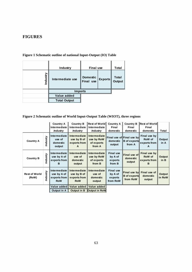
63

FIGURES

Figure 1 Schematic outline of national Input-Output (IO) Table

Figure 2 Schematic outline of World Input-Output Table (WIOT), three regions

Total

In

du

stry

Intermediate use Exports

Industry Final use

Imports

Total Output

Value added

Total Output

Domestic Final use

Output in RoW

Value added Value added Value added

Output in A Output in B Output in RoW

Final use by RoW of

exports from B

Output in B

Rest of World (RoW)

Ind

ust

ry

Intermediate use by A of

exports from RoW

Intermediate use by B of

exports from RoW

Intermediate use of

domestic output

Final use by A of exports

from RoW

Final use by B of exports from RoW

Final use of domestic

output

Final use by B of exports

from A

Final use by RoW of

exports from A

Output in A

Country B

Ind

ust

ry

Intermediate use by A of

exports from B

Intermediate use of

domestic output

Intermediate use by RoW of exports

from B

Final use by A of exports from B

Final use of domestic

output

Country A

Ind

ust

ry

Intermediate use of

domestic output

Intermediate use by B of

exports from A

Intermediate use by RoW of exports

from A

Final use of domestic

output

TotalIntermediate Intermediate Intermediate Final

domestic Final

domestic Final

domestic Industry Industry Industry

Country A Country B Rest of World Country A Country B Rest of World

64

Figure 3 Schematic outline of National Supply-Use table

Figure 4 Schematic outline of International Supply-Use table

Total

Rest of World

Total supply by product (S)

Total input by industry

Imports (M)

Value added (VA)

Exports (E)

Total use by

product (U)

Ind

ust

ry Domestic supply

(SD)

Total output by industry

(GO)

Pro

du

ct

Intermediate use (I)Domestic final

use (F)

Supply Intermediate use Final useProduct Industry

Rest of World (RoW)

Final use

Output

Total supply

Value added

Total use of imports

Intermediate use of

imports

Re-exports

of imports

Total use of

domestic output

Domestic final use of

domestic output

Total Supply

Product

Intermediate use

Industry

country A

Ind

ust

ry

Domestic supply

Pro

du

ct

Rest of World (RoW)

Domestic final use of imports

country A

Pro

du

ct Intermediate

use of domestic

output

Imports

Exports

65

Figure 5 Dataflows and construction steps in WIOT

Public statistics National accounts Supply and use tables

International trade statistics

(time-series) (infrequent) (time-series)

Total Final demand by type Supply (Basic price) Imports and exportsTotal Export and Import Use (Purchasers' price) on bilateral basisValue added by industry - of goodsNet taxes and margins

Gross output by industry - of services

HarmonisationEstimation

Supply (Basic price)Use (Basic price)Valuation matrix

Estimation

Supply (Basic price)Valuation matrix

Domestic use (Basic price)

Estimation

Time series World input-output tables

For each country

Bilateral import shares by use

Import use (Basic price) by delivering country

Time series for each country

Time series for each country

66

Figure 6 Schematic outline of extended National Supply-Use table

   

Total

Capital by typeProfit

Energy use (by type)Air emissions

Natural resources

Ind

us

try

Pro

du

ct

Intermediate use

Domestic supply

Intermediate useSupplyProduct Industry

Final use

Total use by

product

Domestic final use

Total output by industry

Exports

Total supply by product

Total input by industry

Imports

Labour by type

67

Figure 7: Set-Up of a World Supply and Use system (World SUT)

   

Total

Total

Exports to RoW

Exports from A to RoW

Exports from B to RoW

Final domestic

use

Intermediate use

Intermediate use

Industry

Final use by B of imports

from A

Final use of domestic

output

Final use by B of imports from RoW

Country B

Final domestic

use

Intermediate use by B of

imports from RoW

Country B

Rest of World (RoW)

Industry

Pro

du

ct

Intermediate use of

domestic output

Pro

du

ct

Country A

Product Product

Output in A

Final use of domestic

output

Pro

du

ct

Final use by A of imports from B

Final use by A of imports

from RoW

Intermediate use by B of

imports from A

Country A Country ACountry B

Output in A

Value added

Output in B

Intermediate use by A of

imports from B

Intermediate use by A of

imports from RoW

Intermediate use of

domestic output

Value added

Output in B

country A

Ind

ust

ry

Domestic supply

Imports

Country B

Ind

ust

ry

Total supply

Imports

Total supply

Domestic supply

Country A Country B

Supply Supply

68

Appendix Table 1 National supply-use and input-output tables used for construction of WIOD

1995 1996 1997 1998 1999 2000 2001 2002 2003 2004 2005 2006 2007

Australia

SUT (106c * 106i)

SUT (233c *

53i)

SUT (233c *

53i)

Austria

SUT (59c * 59i)

SUT (59c * 59i)

SUT (59c * 59i)

SUT (59c * 59i)

SUT (59c * 59i)

SUT (59c * 59i)

SUT (59c * 59i)

SUT (59c * 59i)

SUT (59c * 59i)

Belgium

SUT (59c * 59i)

SUT (59c * 59i)

SUT (59c * 59i)

SUT (59c * 59i)

SUT (59c * 59i)

SUT (59c * 59i)

SUT (59c * 59i)

SUT (59c * 59i)

Brazil

SUT (110c *

55i)

SUT (110c *

55i)

SUT (110c *

55i)

SUT (110c *

55i)

SUT (110c *

55i)

SUT (110c *

55i)

SUT (110c *

55i)

Bulgaria

SUT (59c * 59i)

SUT (59c * 59i)

SUT (59c * 59i)

SUT (59c * 59i)

SUT (59c * 59i)

Canada

SUT (BP)

(473c*122i)

SUT (BP)

(473c*122i)

SUT (BP)

(473c*122i)

SUT (BP)

(473c*122i)

SUT (BP)

(473c*122i)

SUT (BP)

(473c*122i)

SUT (BP)

(473c*122i)

SUT (BP)

(473c*122i)

SUT (BP)

(473c*122i)

SUT (BP)

(473c*122i)

China

SUT(PR) (40c * 40i) & IO(PR) (124c * 124c)

SUT(PR) (42c * 42i) & IO(PR) (122c * 122c)

SUT(PR) (42c * 42i) & IO(PR) (135c * 135c)

Cyprus*

SUT (59c * 59i)

SUT (59c * 59i)

SUT (59c * 59i)

SUT (59c * 59i)

SUT (59c * 59i)

SUT (59c * 59i)

SUT (59c * 59i)

Czech Republic

SUT (59c * 59i)

SUT (59c * 59i)

SUT (59c * 59i)

SUT (59c * 59i)

SUT (59c * 59i)

SUT (59c * 59i)

SUT (59c * 59i)

SUT (59c * 59i)

SUT (59c * 59i)

SUT (59c * 59i)

SUT (59c * 59i)

Denmark

SUT (59c * 59i)

SUT (59c * 59i)

SUT (59c * 59i)

SUT (59c * 59i)

SUT (59c * 59i)

SUT (59c * 59i)

SUT (59c * 59i)

SUT (59c * 59i)

Estonia

SUT (59c * 59i)

SUT (59c * 59i)

SUT (59c * 59i)

SUT (59c * 59i)

SUT (59c * 59i)

SUT (59c * 59i)

SUT (59c * 59i)

SUT (59c * 59i)

SUT (59c * 59i)

Finland

SUT (59c * 59i)

SUT (59c * 59i)

SUT (59c * 59i)

SUT (59c * 59i)

SUT (59c * 59i)

SUT (59c * 59i)

SUT (59c * 59i)

SUT (59c * 59i)

SUT (59c * 59i)

SUT (59c * 59i)

SUT (59c * 59i)

SUT (59c * 59i)

France

SUT (59c * 59i)

SUT (59c * 59i)

SUT (59c * 59i)

SUT (59c * 59i)

SUT (59c * 59i)

SUT (59c * 59i)

SUT (59c * 59i)

SUT (59c * 59i)

SUT (59c * 59i)

SUT (59c * 59i)

SUT (59c * 59i)

Germany

SUT (59c * 59i)

SUT (59c * 59i)

SUT (59c * 59i)

SUT (59c * 59i)

SUT (59c * 59i)

SUT (59c * 59i)

SUT (59c * 59i)

SUT (59c * 59i)

SUT (59c * 59i)

SUT (59c * 59i)

SUT (59c * 59i)

Greece

SUT (59c * 59i)

SUT (59c * 59i)

SUT (59c * 59i)

SUT (59c * 59i)

SUT (59c * 59i)

SUT (59c * 59i)

SUT (59c * 59i)

Hungary

SUT (59c * 59i)

SUT (59c * 59i)

SUT (59c * 59i)

SUT (59c * 59i)

SUT (59c * 59i)

SUT (59c * 59i)

SUT (59c * 59i)

India

SUT(FC) (115c *

115i)

SUT(FC) (130c *

130i)

SUT(FC) (130c *

130i)

IndonesiaIO (172c * 172c)

IO (175c * 175c)

IO (175c * 175c)

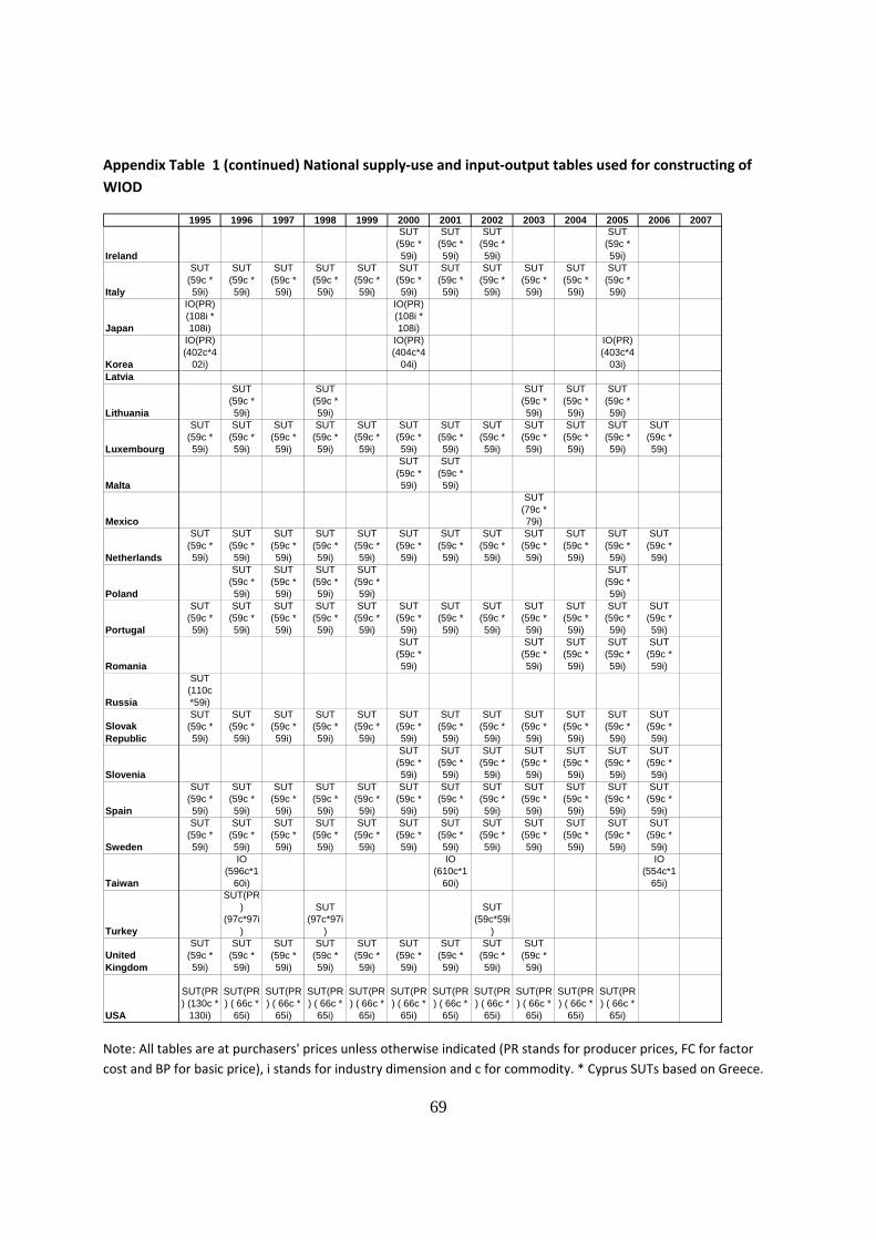
69

Appendix Table  1 (continued) National supply‐use and input‐output tables used for constructing of 

WIOD  

 

Note: All tables are at purchasers' prices unless otherwise indicated (PR stands for producer prices, FC for factor 

cost and BP for basic price), i stands for industry dimension and c for commodity. * Cyprus SUTs based on Greece.  

1995 1996 1997 1998 1999 2000 2001 2002 2003 2004 2005 2006 2007

Ireland

SUT (59c * 59i)

SUT (59c * 59i)

SUT (59c * 59i)

SUT (59c * 59i)

Italy

SUT (59c * 59i)

SUT (59c * 59i)

SUT (59c * 59i)

SUT (59c * 59i)

SUT (59c * 59i)

SUT (59c * 59i)

SUT (59c * 59i)

SUT (59c * 59i)

SUT (59c * 59i)

SUT (59c * 59i)

SUT (59c * 59i)

Japan

IO(PR) (108i * 108i)

IO(PR) (108i * 108i)

Korea

IO(PR) (402c*4

02i)

IO(PR) (404c*4

04i)

IO(PR) (403c*4

03i)Latvia

Lithuania

SUT (59c * 59i)

SUT (59c * 59i)

SUT (59c * 59i)

SUT (59c * 59i)

SUT (59c * 59i)

Luxembourg

SUT (59c * 59i)

SUT (59c * 59i)

SUT (59c * 59i)

SUT (59c * 59i)

SUT (59c * 59i)

SUT (59c * 59i)

SUT (59c * 59i)

SUT (59c * 59i)

SUT (59c * 59i)

SUT (59c * 59i)

SUT (59c * 59i)

SUT (59c * 59i)

Malta

SUT (59c * 59i)

SUT (59c * 59i)

Mexico

SUT (79c * 79i)

Netherlands

SUT (59c * 59i)

SUT (59c * 59i)

SUT (59c * 59i)

SUT (59c * 59i)

SUT (59c * 59i)

SUT (59c * 59i)

SUT (59c * 59i)

SUT (59c * 59i)

SUT (59c * 59i)

SUT (59c * 59i)

SUT (59c * 59i)

SUT (59c * 59i)

Poland

SUT (59c * 59i)

SUT (59c * 59i)

SUT (59c * 59i)

SUT (59c * 59i)

SUT (59c * 59i)

Portugal

SUT (59c * 59i)

SUT (59c * 59i)

SUT (59c * 59i)

SUT (59c * 59i)

SUT (59c * 59i)

SUT (59c * 59i)

SUT (59c * 59i)

SUT (59c * 59i)

SUT (59c * 59i)

SUT (59c * 59i)

SUT (59c * 59i)

SUT (59c * 59i)

Romania

SUT (59c * 59i)

SUT (59c * 59i)

SUT (59c * 59i)

SUT (59c * 59i)

SUT (59c * 59i)

Russia

SUT (110c *59i)

Slovak Republic

SUT (59c * 59i)

SUT (59c * 59i)

SUT (59c * 59i)

SUT (59c * 59i)

SUT (59c * 59i)

SUT (59c * 59i)

SUT (59c * 59i)

SUT (59c * 59i)

SUT (59c * 59i)

SUT (59c * 59i)

SUT (59c * 59i)

SUT (59c * 59i)

Slovenia

SUT (59c * 59i)

SUT (59c * 59i)

SUT (59c * 59i)

SUT (59c * 59i)

SUT (59c * 59i)

SUT (59c * 59i)

SUT (59c * 59i)

Spain

SUT (59c * 59i)

SUT (59c * 59i)

SUT (59c * 59i)

SUT (59c * 59i)

SUT (59c * 59i)

SUT (59c * 59i)

SUT (59c * 59i)

SUT (59c * 59i)

SUT (59c * 59i)

SUT (59c * 59i)

SUT (59c * 59i)

SUT (59c * 59i)

Sweden

SUT (59c * 59i)

SUT (59c * 59i)

SUT (59c * 59i)

SUT (59c * 59i)

SUT (59c * 59i)

SUT (59c * 59i)

SUT (59c * 59i)

SUT (59c * 59i)

SUT (59c * 59i)

SUT (59c * 59i)

SUT (59c * 59i)

SUT (59c * 59i)

Taiwan

IO (596c*1

60i)

IO (610c*1

60i)

IO (554c*1

65i)

Turkey

SUT(PR)

(97c*97i)

SUT (97c*97i

)

SUT (59c*59i

)

United Kingdom

SUT (59c * 59i)

SUT (59c * 59i)

SUT (59c * 59i)

SUT (59c * 59i)

SUT (59c * 59i)

SUT (59c * 59i)

SUT (59c * 59i)

SUT (59c * 59i)

SUT (59c * 59i)

USA

SUT(PR) (130c *

130i)

SUT(PR) ( 66c *

65i)

SUT(PR) ( 66c *

65i)

SUT(PR) ( 66c *

65i)

SUT(PR) ( 66c *

65i)

SUT(PR) ( 66c *

65i)

SUT(PR) ( 66c *

65i)

SUT(PR) ( 66c *

65i)

SUT(PR) ( 66c *

65i)

SUT(PR) ( 66c *

65i)

SUT(PR) ( 66c *

65i)

70

Appendix Table 2 Industries and columns in Use table 

 

 Code NACE Description

1 AtB Agriculture, Hunting, Forestry and Fishing

2 C Mining and Quarrying

3 15t16 Food, Beverages and Tobacco

4 17t18 Textiles and Textile Products

5 19 Leather, Leather and Footwear

6 20 Wood and Products of Wood and Cork

7 21t22 Pulp, Paper, Paper , Printing and Publishing

8 23 Coke, Refined Petroleum and Nuclear Fuel

9 24 Chemicals and Chemical Products

10 25 Rubber and Plastics

11 26 Other Non-Metallic Mineral

12 27t28 Basic Metals and Fabricated Metal

13 29 Machinery, Nec

14 30t33 Electrical and Optical Equipment

15 34t35 Transport Equipment

16 36t37 Manufacturing, Nec; Recycling

17 E Electricity, Gas and Water Supply

18 F Construction

19 50 Sale, Maintenance and Repair of Motor Vehicles Retail Sale of Fuel

20 51 Wholesale Trade and Commission Trade, Except of Motor Vehicles

21 52 Retail Trade, Except of Motor Vehicles ; Repair of Household Goods

22 H Hotels and Restaurants

23 60 Inland Transport

24 61 Water Transport

25 62 Air Transport

26 63 Other Supporting and Auxiliary Transport Activities; Activities of Travel Agencies

27 64 Post and Telecommunications

28 J Financial Intermediation

29 70 Real Estate Activities

30 71t74 Renting of M&Eq and Other Business Activities

31 L Public Admin and Defence; Compulsory Social Security

32 M Education

33 N Health and Social Work

34 O Other Community, Social and Personal Services

35 P Private Households with Employed Persons

36 Financial intermediation services indirectly measured (FISIM)

37 Total

38 Final consumption expenditure by households

39 Final consumption exp. by non-profit organisations serving households

40 Final consumption expenditure by government

41 Final consumption expenditure

42 Gross fixed capital formation

43 Changes in inventories and valuables

44 Gross capital formation

45 Exports

46 Final uses at purchasers' prices

47 Total use at purchasers' prices

Columns in USE Table

71

Appendix Table 3 Products and rows in Use table 

 

  Code CPA Description

1 1 Products of agriculture, hunting and related services

2 2 Products of forestry, logging and related services

3 5 Fish and other fishing products; services incidental of fishing

4 10 Coal and lignite; peat

5 11 Crude petroleum and natural gas; services incidental to oil and gas extraction excluding su

6 12 Uranium and thorium ores

7 13 Metal ores

8 14 Other mining and quarrying products

9 15 Food products and beverages

10 16 Tobacco products

11 17 Textiles

12 18 Wearing apparel; furs

13 19 Leather and leather products

14 20 Wood and products of wood and cork (except furniture); articles of straw and plaiting mate

15 21 Pulp, paper and paper products

16 22 Printed matter and recorded media

17 23 Coke, refined petroleum products and nuclear fuels

18 24 Chemicals, chemical products and man-made fibres

19 25 Rubber and plastic products

20 26 Other non-metallic mineral products

21 27 Basic metals

22 28 Fabricated metal products, except machinery and equipment

23 29 Machinery and equipment n.e.c.

24 30 Office machinery and computers

25 31 Electrical machinery and apparatus n.e.c.

26 32 Radio, television and communication equipment and apparatus

27 33 Medical, precision and optical instruments, watches and clocks

28 34 Motor vehicles, trailers and semi-trailers

29 35 Other transport equipment

30 36 Furniture; other manufactured goods n.e.c.

31 37 Secondary raw materials

32 40 Electrical energy, gas, steam and hot water

33 41 Collected and purified water, distribution services of water

34 45 Construction work

72

Appendix Table 3 Products and rows in Use table (continued) 

 

  

   

35 50 Trade, maintenance and repair services of motor vehicles and motorcycles; retail sale of a

36 51 Wholesale trade and commission trade services, except of motor vehicles and motorcycle

37 52 Retail trade services, except of motor vehicles and motorcycles; repair services of person

38 55 Hotel and restaurant services

39 60 Land transport; transport via pipeline services

40 61 Water transport services

41 62 Air transport services

42 63 Supporting and auxiliary transport services; travel agency services

43 64 Post and telecommunication services

44 65 Financial intermediation services, except insurance and pension funding services

45 66 Insurance and pension funding services, except compulsory social security services

46 67 Services auxiliary to financial intermediation

47 70 Real estate services

48 71 Renting services of machinery and equipment without operator and of personal and house

49 72 Computer and related services

50 73 Research and development services

51 74 Other business services

52 75 Public administration and defence services; compulsory social security services

53 80 Education services

54 85 Health and social work services

55 90 Sewage and refuse disposal services, sanitation and similar services

56 91 Membership organisation services n.e.c.

57 92 Recreational, cultural and sporting services

58 93 Other services

59 95 Private households with employed persons

60 Total

61 Cif/ fob adjustments on exports

62 Direct purchases abroad by residents

63 Purchases on the domestic territory by non-residents

64 Total intermediate consumption/final use at purchasers' prices

65 Compensation of employees

66 Other net taxes on production

67 Operating surplus, gross

68 Value added at basic prices

69 Output at basic prices

73

 

 

Appendix 4 BEC correspondence

End use category BEC rev.3 Description100 Food and beverages 110 ...Primary

Intermediate 111 ......Mainly for industry Consumption 112 ......Mainly for household consumption

120 ...Processed Intermediate 121 ......Mainly for industry Consumption 122 ......Mainly for household consumption

200 Industrial supplies not elsewhere specified Intermediate 210 ...Primary Intermediate 220 ...Processed

300 Fuels and lubricants Intermediate 310 ...Primary

320 ...Processed Not classified 321 ......Motor spirit Intermediate 322 ......Other

400 Capital goods (except transport equipment), and parts and accessories thereof Capital goods 410 ...Capital goods (except transport equipment) Intermediate 420 ...Parts and accessories

500 Transport equipment and parts and accessories thereof Not classified 510 ...Passenger motor cars

520 ...Other Capital goods 521 ......Industrial Consumption 522 ......Non-Industrial Intermediate 530 ...Parts and accessories

600 .Consumer goods not elsewhere specified Consumption 610 ...Durable Consumption 620 ...Semi-durable Consumption 630 ...Non-durable Not classified 700 Goods not elsewhere specified