Multiregional Input-Output Database

OPEN:EU Technical Document

one planeteconomy network

Page 1 of 23

OPEN:EU

Multiregional Input-Output Database

TECHNICAL DOCUMENT

TRONDHEIM, 25 JUNE 2010

Edgar G. Hertwich1 and Glen P. Peters1,2

1 Industrial Ecology Programme, Norwegian University of Science and Technology, Trondheim, Norway

2 CICERO, Oslo, Norway

7th Framework Programme for Research and Technological Development

The research leading to these results has received funding from the European Community's Seventh

Framework Programme (FP7/2007-2013) under grant agreement N° 227065. The contents of this

report are the sole responsibility of the One Planet Economy Network and can in no way be taken to

reflect the views of the European Union.

Page 2 of 23

Index

1. Introduction ......................................................................................................... 3

2. Multi-regional Input-Output Analysis (MRIO) ...................................................... 5

3. Common assumptions in MRIO ............................................................................. 8

Uni-directional trade ............................................................................................ 8

Import assumption .............................................................................................. 9

Others ................................................................................................................ 9

4. Practical issues .................................................................................................. 10

Grouping of like regions ...................................................................................... 10

Using trade shares to estimate ijA ....................................................................... 10

Exchange rates.................................................................................................. 11

Inflation ........................................................................................................... 11

Product or industry classifications ........................................................................ 11

Re-classifying data ............................................................................................. 11

Aggregation ...................................................................................................... 12

Valuation .......................................................................................................... 12

Marginal technology ........................................................................................... 13

Errors............................................................................................................... 13

5. Evaluation of available MRIO data sources ......................................................... 14

General data availability ..................................................................................... 14

MRIO data choice in OPEN:EU ............................................................................. 14

6. Example applications and policy implications ..................................................... 16

Trans-boundary pollution .................................................................................... 16

Arbitrary demands ............................................................................................. 17

Priority setting for nations and regions ................................................................. 17

7. Acknowledgements ............................................................................................ 18

8. References ......................................................................................................... 19

9. Appendix: GTAP7 Country and sector detail ....................................................... 22

Page 3 of 23

1. Introduction

Multiregional input-output analysis (MRIO) is increasingly used to analyse the environmental

implications of consumption, be it for greenhouse gas emissions, land use, and water use.

Input-output tables display the interconnection between different sectors of production and

allow for a tracing of the production and consumption in an economy. Traditionally, input-

output tables are constructed for national economies; however, production is increasingly

global. Already in 2001, 22% of global CO2 emissions were associated with the production for

goods traded internationally. Hence, multi-regional input-output tables – including the trade

between different countries –have become attractive for representing the global aspects of our

consumption (Andrew et al. 2009; Druckman and Jackson 2009; Lenzen et al. 2010;

Wiedmann 2009a, 2009b; Wiedmann et al. 2010; Wilting and Vringer 2009; Hertwich and

Peters 2009; Weber and Matthews 2008; Peters 2008).

The unique feature of a MRIO is that it allows the tracing of the production of a “typical

product” of economic sectors, quantifying the contributions to the value of the product from

different economic sectors in various countries represented in the model. It hence offers a

description of the global supply chains of products consumed. If the specific use of land,

energy, and water, and emissions of the industry sectors in each country are known, the total

land, carbon and water footprints of the products can be quantified.

In the OPEN:EU project, a MRIO is used to assess the environmental footprints of products,

supplemented by more specific accounting methods for the production of agricultural products

which are particularly important for land and water use. This report is written to document the

MRIO modeling methods used in the OPEN:EU project. It also provides a short discussion of

the choice of a particular data set (GTAP vs. EXIOPOL) and some comments on the GTAP7

model. It is targeted at scientists who would like to understand the underlying methods and

data considerations used to construct the footprint analysis for OPEN:EU. It also serves as

introduction and documentation for those who will maintain and update the EUREPA tool that

will be build in the project.

Consumption causes environmental impacts in two different ways. Direct environmental

impacts result from consumption when consumers directly burn fossil fuels; for instance, from

the petrol used for personal transportation or wood used for space heating. Significant

environmental impacts also occur indirectly in the production of consumable goods. When

production occurs in the same country as consumption, then government policy can be used to

regulate environmental impacts. However, increasing competition from imported products has

led to a large share of production occurring in a different country to consumption. Regulating

the resulting pollution embodied in trade is becoming critical to stem global pollution levels.

Due to increased globalization of production networks, there is increasing interest in the effects

of trade on the environment (c.f. Jayadevappa and Chhatre, 2000; Copeland and Taylor,

2003).

With the increased interest in trade and the environment research activity is focusing on

methods of accurately calculating the pollution embodied in traded products. Early studies in

this area assumed that imports were produced with the same technology as the domestic

economy (e.g. Wyckoff and Roop, 1994; Lenzen, 1998; Kondo et al., 1998; Battjes et al.,

1998; Machado et al., 2001), however, using this assumption large errors may result when the

countries have diverging technology and energy mixes (Lenzen et al., 2004; Peters and

Page 4 of 23

Hertwich, 2006a,c)1. This stimulated research in the use of multi-regional input-output (MRIO)

models. While MRIO models have been applied to regional economics since the 1950’s (Miller

and Blair, 1985), applications to environmental problems has only recently emerged (Chung

and Rhee, 2001; Ahmad and Wyckoff, 2003; Lenzen et al., 2004; Nijdam et al., 2005; Peters

and Hertwich, 2006a,b; Guan and Hubacek, 2006; Wiedmann, T. 2009b). These studies are

finding large portions of pollution embodied in trade. For instance, Ahmad and Wyckoff, 2003

found that the emissions embodied in trade was on average 14% in OECD countries and over

50% in some OECD countries; they included data covering 80% of global emissions and use

“conservative” assumptions to obtain a lower bound. Further, Ahmad and Wyckoff, 2003 found

that “emissions embodied in international trade are important, growing, and likely to continue

to grow”.

Full multi-region models endogenously combine domestic technical coefficient matrices with

import matrices from multiple countries or regions into one large coefficient matrix, thus

capturing trade supply chains between all trading partners as well as feedback effects. The

latter are changes in production in one region that result from changes in intermediate

demand in another region, which are in turn brought about by demand changes in the first

region.

In this report we discuss the theory behind MRIO models for applications in footprint

calculations (Section 2) and discuss common modeling assumptions (Section 3). MRIO models

require a considerable amount of data and we discuss many of the practical data issues that

are encountered in MRIO modeling (Section 4). In Section 5 we briefly review important

applications of MRIO in environmental policy making. In Section 6 we finally discuss the

potential for increased use of MRIO models to indicate the type of policy questions the

OPEN:EU model could be used to answer (section 6).

1 Similar conclusions are found in the economic literature on factors (labor and capital) embodied in trade (Hakura,

2001).

Page 5 of 23

2. Multi-regional Input-Output Analysis (MRIO)

Using IOA the total output of the domestic economy is given by2

x Ax y (1)

where A is the total inter-industry requirements and y is the total net demand on the

economy,

d exy y y m (2)

where dy are the products produced and consumed domestically,

exy are the products

produced domestically, but consumed in foreign regions (exports), and m are the products

consumed domestically for both final and intermediate consumption, but produced in foreign

regions (total imports). In this form, (1) is not suitable for applying arbitrary demands since

imports are embedded in both A and y (Dietzenbacher et al., 2005).

It is possible to separate the domestic and imported components in A and y to obtain

( )d im d ex imx A A x y y y m (3)

where dA is the industry requirements of domestically produced products per unit output,

imA

is the industry requirements of imported products per unit output, and imy is the final demand

of imports (United Nations, 1999). A balance must hold for the total imports,

im imm A x y (4)

and thus (1) can be reduced to domestic activity only,

d d ex d tx A x y y A x y (5)

Using the linearity assumption of IOA, it follows that the output of the domestic economy for

an arbitrary demand is

1( )dx I A y (6)

where y could represent household demand, government demand, a unit demand on a

particular sector, and so on. Given the domestic output, the requirement of imports by

industry to produce y are given by

imA x . This import may instigate a series of feedbacks

through trade flows and is discussed further below.

Using the direct multiplier for environmental impacts3 per unit output, F , the environmental

impacts embodied in domestic consumption are,

1( )df F I A y (7)

This equation does not include the environmental impacts that may occur in foreign regions

due to imports.

Particularly for environmental impacts with global implications, such as global warming, it is

important to calculate the global environmental impacts for production and consumption.

Imports are generally produced in countries with different production technologies and energy

mixes compared to the domestic economy. This suggests that a multi-regional model is

required to correctly evaluate the pollution embodied in traded products. When trade is

2 This section and selected parts of this document are based on Peters and Hertwich, 2009. 3 The same equation applies for the standard economic factors of production such as labor and capital.

Page 6 of 23

allowed between two or more countries trade feedbacks may occur so that production in one

country, may require some of its own production via feedback loops (see Figure 1a). This type

of interaction can be analyzed using MRIO.

Table 1. The notation used for the MRIO model.

Name Description

ix Output of region i .

iiy Final demand for goods produced and consumed in i .

ijy Final demand from region i to region j .

1

mex

i ijj j iy y

Total final demand exports from region i .

iiA Interindustry requirements on domestic production in region i .

ijA Interindustry requirements from region i to j .

i ijjA A Total interindustry requirements in region i .

ij ij j ijm A x y Total trade from region i to region j .

iF Direct factor requirements in region i .

An MRIO model extends the standard IO matrix to a larger system where each industry in each

country has a separate row and column. If there are m regions then the extended IO matrix

becomes4

11 11 112 13 11 1

221 22 232 2 21

331 32 333 3 31

1 2 3 1

exm

m

m

m mmm mm m m

A A A … Ax x y y

A A A … Ax x y

A A A … Ax x y

A A A … Ax x y

(8)

The notation is described in Table 1. We have simplified the system by centering the model on

the domestic economy, 1i . Due to symmetry, any region can be considered as the domestic

economy by re-labeling it as region 1. The block matrices of the extended IO table represent

the global technology. The diagonal block matrices represent domestic interindustry

requirements and the off-diagonal elements represent the interindustry requirements of traded

products.

For some it may be easier to understand the MRIO model with separate equations. The output

in the domestic economy is

1 11 1 11 1 1

1

exports

for 1j j j

j

x A x y A x y i

(9)

where the export terms are all exports from region 1 to interindustry and final demand in all

other regions. The outputs in the other regions are,

4 Peters and Hertwich, 2004 build the MRIO equations from a 2-region system and is useful for those that may require

a more detailed description of how the equations are derived.

Page 7 of 23

1

exports

for all 1i ii i ij j i

j i

x A x A x y i

(10)

Since region 1 is treated as the domestic economy, the final demands 1iy are imports to region

1.

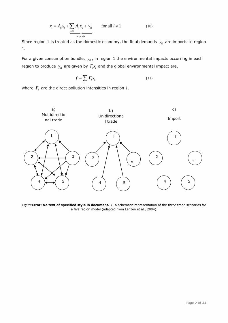
For a given consumption bundle, 1iy , in region 1 the environmental impacts occurring in each

region to produce 1iy are given by i iF x and the global environmental impact are,

i i

i

f F x (11)

where iF are the direct pollution intensities in region i .

FigureError! No text of specified style in document.-1. A schematic representation of the three trade scenarios for

a five region model (adapted from Lenzen et al., 2004).

5

3

1

2

3

4 5

1

2

4

c)

Import

assumptio

n

b)

Unidirectiona

l trade

1

2 3

4 5

a)

Multidirectio

nal trade

Page 8 of 23

3. Common assumptions in MRIO

To perform an MRIO study requires a considerable amount of data, much of which is not

directly available. Consequently, most current applications of environmental MRIO have

applied some approximations to (8). In this section we discuss various approximations and

simplifications that have been used in environmental MRIO. The following is largely based on

Ahmad and Wyckoff, 2003; Lenzen et al., 2004; Peters and Hertwich, 2004; Nijdam et al.,

2005; Peters and Hertwich, 2006a,b. Practical issues associated with data availability and

handling are discussed in Section 4.

Uni-directional trade

If it is assumed that the domestic economy trades with all regions, but the other regions do

not trade amongst each other (see Figure 1b), then the data requirements are greatly reduced

without introducing large errors. Lenzen et al., 2004 found these effects to be around 1-4%

(see their Table 7) and these terms are often assumed to be negligible in other regional

models (Round, 2001).

Mathematically, the uni-directional trade assumption reduces (8) to,

1 11 1 11 1

212 22 2 21

31 333 3 31

1 1

0 0 0

0 0

0 0

0 0

ex

m m mm m m

x A … x y y

x A A … x y

x A A … x y

x A … A x y

(12)

Since this assumption reduces many of the feedback loops, the equation can be solved directly

to obtain,

1

1 11 11 1( ) exx I A y y

(13)

for the domestic economy and the output in the other regions are

1( ) for 1i ii ix I A M i (14)

where

1 1 1i i iM A x y (15)

The exports term 1

exy now includes both exports to final demand and exports to industry. This

approach has been applied by Nijdam et al., 2005; Peters and Hertwich, 2006a,b, and (Weber

and Matthews 2008).

If only analyzing the total final demand on an economy, the uni-directional trade assumption

does not require ijA . If the total final demand is used, then (15) gives the total imports into

the domestic economy and so iM can be obtained directly from IO or trade data.

The assumption of uni-directional trade gives two options for the diagonal terms of the foreign

regions. If 1iiA i is placed on the diagonal, then multi-directional trade is totally neglected.

Page 9 of 23

Alternatively, if 1iA i is placed on the diagonal, then multi-directional trade is included, but

with the assumption that imports are produced with domestic technology (see Section 3.2).

However, the country that is allocated the emissions for the production of the imports will be

incorrect. Due to data availability, countries may only supply iA in which case it is implicitly

assumed that multi-directional trade is included using domestic technology.

Import assumption

A common assumption is that imports are produced with domestic production technology

(Figure 1c). The import assumption has also been called “autonomous regions” by Lenzen et

al., 2004 and “mirrored economy” by Strømman and Gauteplass, 2004. The assumption

greatly reduces data requirements, but may lead to large errors. Lenzen et al., 2004 found the

error between the import assumption and multi-directional trade for Danish CO2 emissions to

be 20-50% depending on the final demand. Peters and Hertwich, 2006a found the difference

between the import assumption and uni-directional trade for Norwegian household

consumption to be a factor of 2.7 for CO2, 9.7 for SO2, and 1.5 for NOx. Most IO studies of

environmental issues apply the import assumption and so it is likely that many of these studies

incorrectly calculate the emissions associated with the production of imports.

One way to apply the import assumption is to assume 11iiA A , 1ij iA A , and 1iF F and then

substitute into (8). Simplification then results in,

1

1( )i ix I A y (16)

where iy is the final demand placed on each region (Peters and Hertwich, 2004). This

equation gives the emissions in each region, including imports to industry, but it assumes they

have the same production technology as the domestic economy and allocates the embodied

emissions to the domestic economy. The correct allocation can be obtained by using (8), but

with substitution of 11iiA A and 1ij iA A .

Others

Some approaches have been slightly different to what is outlined above. Ahmad and Wyckoff,

2003 do not use the matrix based approach we have described above, but use an iterative

procedure which approximates the matrix solution. Lenzen et al., 2004 replace each of the

block matrices with a make and use block which displays additional structure, but applies an

industry-technology assumption on solution. Methods not using IOA to estimate pollution

embodied in trade often neglect indirect emissions in the production chain and are

consequently not considered in this article.

Page 10 of 23

4. Practical issues

A significant amount of data from a variety of sources is required to perform an MRIO study.

As a consequence several practical issues arise in the data manipulation phase. This section

briefly discusses the main areas of concern. Lenzen et al., 2004 also give a detailed discussion

of some of these issues.

Grouping of like regions

Two approaches have been used in the past to fill in for missing IO data. A first approach is to

allocate the countries without IO data the IO data of a “representative” country. Ahmad and

Wyckoff, 2003 used the United States of America and Lenzen et al., 2004 used Australia as the

representative country. Another approach is to collect IO data for the most significant trading

partners and then allocate the minor trading partners to one of the major trading partners to

make larger aggregated regions with fixed technology. This approach was applied by Peters

and Hertwich 2006a,b and the allocation was performed based on energy use per capita, CO2

emissions per capita, and gross domestic product per capita. If the major trading partners

represent a diverse range of economies, then the second approach is likely to give a better

approximation. In both approaches, it is also possible to adjust emission coefficients if the data

is available; for example, when allocating emissions data between countries Ahmad and

Wyckoff, 2003 adjusted the emission coefficient for electricity production based on other

reliable data sources (also see Battjes et al., 1998).

Using trade shares to estimate ijA

Data on ijA and ijy is generally not directly available; however, many countries construct

im

i ijj iA A

and

im

i ijj iy y

. Using

im

iA together with trade flow data it is possible to

estimate the share of trade flows to final demand and industry in each region using

ˆ im

ij ij iA s A (17)

and

ˆ im

ij ij iy s y (18)

where

ij k

ij kiji k

ms

m

(19)

where ij k

m

is the total imports of product k from region i to j. It is important to consider the

trade shares in individual sectors and not the average of all sectors. More details on using

trade shares to estimate ijA can be found in Lenzen et al., 2004.

Page 11 of 23

Exchange rates

In an MRIO model, exchange rates are needed to link the data from different regions to a

common currency. There has been considerable debate in the climate change literature about

the use of Purchasing Power Parities (PPP) or Market Exchange Rates (MER) in currency

conversation (Castles and Henderson, 2003; Grübler et al., 2004; Nordhaus, 2005). The MER

is calculated based on traded products, while the PPP is calculated based on a bundle of

consumed products; both traded and non-traded. The PPP rates give a better measure of

income levels across different countries. Much of the debate about PPP and MER has been

based on the comparison of income levels and not a comparison of traded products. Since

MRIO models focus on traded products we suggest the use of MERs to obtain a common

currency. It is possible to avoid the exchange rate problems by using physical units for key

sectors; however, data in physical units requires additional data issues, particularly availability.

Inflation

The data covering a variety of regions is likely to come from various time periods. Adjustments

for inflation are required to make the data consistent for a given base year. The easiest

approach is to use the Consumer Price Index (CPI) in each country to adjust for inflation.

However, the CPI is likely to introduce other errors. The CPI is an aggregated index, while

price changes are likely to be different in each of the IO sectors. Further, the CPI also varies

depending on the base year used and the method of indexing applied. These issues are difficult

to resolve and the errors will be greater for a large CPI and when there is a big difference in

base years.

Product or industry classifications

It is possible to perform IOA using a product classification or an industry classification.

Through the make and use system it is possible to transfer between the two using the make

matrix. The emissions data is usually in an industry classification and the final demand,

depending on the application, will be either an industry or product classification. Consequently,

for some studies there will be a need to map between the industry and product classifications.

Given that the emissions data is always in an industry classification and IO tables are often

only supplied in an industry classification we suggest using industry classifications as this

requires less data manipulations. This would imply mapping the final demands in a product

classification into the industry classification using the make matrix.

Re-classifying data

The IO data from different regions is often in different classification systems. To perform the

analysis requires mapping the data, at some stage, to a consistent classification. For some

classifications it is possible to obtain correspondence tables, otherwise, the correspondence

tables need to be constructed by referring to the different classification descriptions. Often, the

classification systems do not have a direct correspondence between sectors and while the

classification definitions can be used as a guide, re-classification will nearly always introduce

errors of unknown size.

Page 12 of 23

Another issue is that some data is collected based on entirely different conceptual framework.

For example, IO data in an industry classification is based on industries being the smallest

unit, while consumer expenditure survey data is collected on the basis of products and

functions being the smallest unit (the classification of individual consumption by purpose

(COICOP) is a good example). Mapping between products or functions and industries is difficult

implying that several assumption and approximations are required. In some cases checks can

be applied. For example, when mapping consumer expenditure data to an industry

classification, it is possible to ensure that a rough balance is obtained at the sector level

between the mapped expenditure data and the household expenditure from the IO tables.

Aggregation

In the MRIO setting, Lenzen et al., 2004 show the importance of aggregation errors with the

broad conclusion that the data should be in the highest detail available. Thus, a global MRIO

with 10-sector aggregation, for example, may produce unreliable results. The required sector

detail depends on the use of the model.

Valuation

IO data is often available in three levels of valuation; basic, producer, or purchaser (retail)

prices. The different valuations differ in the trade and transport margins, and taxes and

subsidies; producer = basic + taxes - subsidies, purchaser = producer + margins. Typically

margins and taxes are applied at different rates in different sectors and on different products.

Even across the same product, margins and taxes can differ for a variety of reasons such as,

different mark-ups, different modes of transport, different levels of taxation, bulk discounts,

different recording principles, and so on (United Nations, 1999). For these reasons it is more

homogenous to work in basic prices as they are more representative of the production value of

a product compared to the market value.

Unfortunately, not all IO data is available in basic prices. Estimation can be used to adjust the

IO data to the required valuation, but without the detailed data in each sector, the possibility

for introducing large errors is considerable. Due to data availability, it is likely to be easier to

convert the final demand to a new valuation compared to the IO data. In practice, if data is not

available in the necessary valuation, it may be best to report the valuation of the data and

emphasis that it will either under- or over-estimate the environmental impacts depending on

the valuation used.

An addition problem arises in the valuation of trade data. Exports are usually presented as free

on board (fob) and imports as cost, insurance, freight (cif). For consistency, the imports need

to be converted to basic prices. Lenzen et al., 2004 use economy wide fob/cif ratios and then

balance the resulting MRIO table using a RAS technique.

Page 13 of 23

Marginal technology

It can be argued that the regional technology differences are not relevant in some studies.

Instead, any expanded production will occur with marginal technology (Weidema et al., 1999;

Ekvall and Weidema, 2004). If modeling past flows, then the technology used in production is

required. In the modeling of future scenarios it is important to consider the likely technology

mix and emissions coefficients in the future; in this case, marginal technologies may be

preferred. A possible alternative is to consider the energy embodied in trade as the energy

intensities are less dependent on the fuel mix (Peters and Hertwich, 2005a).

Errors

Errors can enter into the calculations in many ways. The IO data and factor use intensities

always have an error associated with them (e.g., Rypdal and Zhang, 2000; Lenzen, 2001;

Yamakawa and Peters 2009, Lenzen et al. 2010). Errors also arise in the adjustments for

currency conversions, inflation, different sector classifications, aggregation, and so on. The

magnitude of these errors is often difficult to estimate, but the errors still need to be

considered (Morgan and Henrion, 1990). Ideally, some sort of error analysis should be

performed or the potential magnitude of uncertainties discussed.

Page 14 of 23

5. Evaluation of available MRIO data sources

General data availability

To perform a detailed MRIO study IO data is essentially required for every country. This data is

generally available for most OECD countries, but for relatively few non-OECD countries. Most

EU countries submit data to Eurostat in a consistent format. The USA, Canada, and Australia

regularly compile IO data but using different classifications. The data availability in non-OECD

countries is sparse and often for major non-OECD countries only. Some data projects have

attempted to build large IO databases for global models.

Emissions data is often available for countries that supply IO data, but in many cases the data

needs separate construction. Energy data can be used to construct some air emissions data

(e.g., Ahmad and Wyckoff, 2003; Dimaranan and McDougall, 2006) alternatively, additional

data work may be required (e.g., Suh, 2005; Guan and Hubacek, 2006). Care needs to be

taken with energy and environmental data from some sources as they may have a different

system boundary to the IO data (Gravgård Pedersen and de Haan, 2006; Peters and Hertwich,

2006c). Energy and emissions data are often constructed according to “national territory”,

while IO data are constructed according to “resident institutional units”. Resident institutional

units may operate and pollute outside national territory, but are still a part of the domestic

economy. The main differences between the two definitions are for international transportation

and tourist activities. For Denmark in 2001 the differences between the two definitions were

23% for CO2, 93% for SO2 and 72% for NOx (Gravgård Pedersen and de Haan, 2006). For

Norway in 2000 the difference was 25% for CO2 (Peters and Hertwich, 2006c).

Trade data is available from several sources, but generally trade data has missing data and

mismatches. This requires addition processing and cross-checking for consistency (e.g.,

Dimaranan and McDougall, 2006). Import and export data often do not match due to different

pricing conventions and errors in reporting. If traded goods between two countries go through

a third country then allocation problems often arise.

MRIO data choice in OPEN:EU

For the OPEN:EU project, we have considered two principal data sources for MRIO data: The

Global Trade, Assistance, and Production project (GTAP) and the EXIOPOL project (A new

environmental accounting framework using externality data).

Table 2 provides an overview over important characteristics of the two data sources.

For GTAP, we consider both release 6 and release 7. GTAP7 provides data for 113 world

regions in 57 sector detail (Narayanan G. and Walmsley, 2008). It has the most extensive

regional coverage. It is a well-recognized database that has been used extensively for trade

analysis, agricultural economics and tariff issues, and recently also for carbon footprint

analysis (Hertwich & Peters, 2009). While the GTAP database is extensive and has a more

recent reference year, it must be noted that the actual data utilized is often from earlier years

and has only been adjusted to the activity in the reference year. The data for individual regions

is usually submitted by users of the data and consequently data is sometimes not updated with

new versions of the database. The database has a strong emphasis on food and agriculture.

This is a particularly useful feature for the OPEN: EU project as both Ecological and Water

Footprint of calculations are mainly based on data for agricultural products. More agricultural

Page 15 of 23

sectors in the IO model allow for a more accurate allocation of bioproducts. The increase in

regional coverage from version 6 to 7 is also welcome. It should be noted that in version 7.1, a

harmonized set of EU27 input-output data was introduced based on the work of the EC Joint

Research Center in Seville (IPTS), which provides for an improved data situation for EU

countries.

The rationale of the EXIOPOL project is to provide an MRIO database specifically for

environmental analysis, with more detail on the environmentally relevant sectors (agriculture,

energy, materials) and environmental extensions describing the energy, material and land use,

as well as emissions of greenhouse gases and air pollutants and some other pollutants to cover

important contributions to environmental impact indicators as used in life-cycle assessment

(Tukker et al. 2009). In addition, the manipulation of the input-output tables should not be as

extensive as in GTAP, preserving to some degree the underlying IO tables published for the

individual countries. Disadvantages with EXIOPOL are that fewer countries are covered, that

the reference year 2000 is earlier than that for GTAP7 (2004) and that the database has not

yet been used as extensively and hence has not yet the international recognition that GTAP

has. Furthermore, the use of GTAP data will facilitate comparisons with results (for the carbon

footprint) from previous studies and other research groups.

Based on these considerations, we originally suggested the use of the EXIOPOL database for

OPEN:EU. However, the completion of the database has suffered some setbacks and had to be

delayed. The database is hence not yet ready at a time we need to proceed with the OPEN:EU

project. For this reason, we have reconsidered our earlier recommendation and now implement

the GTAP7 database. In principle, the work in WP1 and WP2 has been structured in a manner

that would allow the implementation of the EXIOPOL database in the same scripts and with the

same footprint data as the GTAP database. Whether this remains feasible within the time

horizon and effort reserved for this project remains to be seen. As mentioned above, there is a

trade-off in advantages of using one database over the other and it is important to note that

using GTAP instead of EXIOPOL does not have any effect on the ability of the OPEN:EU project

to deliver all of its aims.

In the appendix, the sectors and countries represented in GTAP7 are described.

Table 2. Overview of the characteristics of global MRIO datasets considered for OPEN:EU

GTAP6 GTAP7 EXIOPOL

Published 2006 2008 Winter 2010/11

Base year 2001 2004 2000

No. of countries 87 113 EU27+16 (1)

No. of sectors 57 57 128

Environmental extensions GHG GHG GHGs, air pollution, land use, material extraction

Environmental detail agricultural sectors agriculture, energy + material sectors presented

(1) US, Japan, China, Canada, South Korea, Brazil, India, Mexico, Russia, Australia,

Switzerland, Turkey, Taiwan, Norway, Indonesia and South Africa.

Page 16 of 23

6. Example applications and policy implications

Generally, there are three scales of interest in consumption related issues; national, regional,

and local (Munksgaard et al., 2005). In the context of this article we will consider two scales;

total demand (national and global) and arbitrary demand (regional and local). Most

applications of MRIO have been to address global issues of pollution embodied in trade and the

carbon footprint of nations. Only recently have MRIO studies considered arbitrary demands. In

this section, we outline the main applications of MRIO in the field of industrial ecology. We do

not consider studies that have modeled similar questions, but using single region models with

the import assumption.

Trans-boundary pollution

The main motivation for the studies by Chung and Rhee, 2001; Ahmad and Wyckoff, 2003;

Lenzen et al., 2004; Peters and Hertwich, 2006c was to evaluate pollution embodied in trade

at the national level and to determine the different environmental impacts of consumption

versus production and its implications to global climate change policy (Kondo et al., 1998;

Munksgaard and Pedersen, 2001; Bastianoni et al., 2004). These studies generally found a

large portion of CO2 emissions embodied in trade. The most comprehensive early study,

Ahmad and Wyckoff, 2003, found that the CO2 emissions embodied in imports in some OECD

countries was over 50% and on average 14% of OECD CO2 emissions were embodied in

imports. However, the authors used conservative assumption such as not including services

trade, excluding process emissions, and intentionally making assumptions that led to a lower

bound. It is likely that these numbers are larger in reality. Lenzen et al., 2004 found that 66%

of Danish domestic CO2 emissions in 1997 were embodied in imports, which is considerably

greater than the value of 36% found by Ahmad and Wyckoff, 2003. Peters and Hertwich,

2006c found that 67% of Norwegian domestic CO2 emissions in 2000 were embodied in

imports, which is similar to the value of 54% found by Ahmad and Wyckoff, 2003 for 1997.

The reason for the differences are unknown, but may be since Ahmad and Wyckoff, 2003 used

different assumptions and data set. Chung and Rhee, 2001 used an MRIO for trade between

Japan and Korea, but they did not consider the pollution embodied in imports from outside of

Japan and Korea. Their study has a regional focus for trade between Japan and Korea, but not

on the global implications.

More recently, Peters and Hertwich (2008) and Davis and Caldeira (2010) have analysed the

CO2 emissions embodied in international trade based on the GTAP 6 and GTAP7 databases,

respectively. They found that high-density OECD countries had higher emissions embodied in

imports than exports, while for raw materials exporters like Russia, Canada, Australia, Finland,

Norway and South Africa, the situation was the reverse. Emerging economies specializing in

manufacturing, like China and India also had higher emissions embodied in exports and

imports.

Guan and Hubacek, 2006 consider virtual water flows5 between south and north China using

an MRIO model. They found that the water scarce north exports large quantities of virtual

water to the relatively water abundant south. Guan and Hubacek, 2006 go on to show that this

contradicts the standard theory of comparative advantage; often referred to as the “Leontief

paradox”. This highlights the wider applications of MRIO models to any factor of production

embodied in trade (also see Hakura, 2001).

5 Guan and Hubacek, 2006 refer to embedded water content as “virtual water".

Page 17 of 23

Arbitrary demands

The studies by Nijdam et al., 2005; Peters and Hertwich, 2005b; 2006a focus on the

implication of imports for household environmental impacts (HEI). Both use MRIO models with

uni-directional trade only, Nijdam et al., 2005 consider nine environmental indicators for Dutch

household consumption, while Peters and Hertwich, 2005b; 2006a consider CO2, SO2, and NOx

emissions for different Norwegian final demands. Both studies found that large fractions of HEI

are embodied in imports directly to households and imports to domestic industries as inputs to

produce domestic household demand. Except for traffic noise (Dutch study) and NOx

(Norwegian study) over 50% of the measured global HEI were embodied in imports;

greenhouse gases were around 50% in both cases. In many cases the environmental impacts

from developing countries was most significant, particularly considering the smaller share of

imports coming from those regions. Both studies reinforced the overall importance of mobility

and food in HEI (c.f. Hertwich, 2005), but found increased importance of consumable items

due to imports. The Norwegian study found that for food, business services, clothing,

chemicals, furniture, cars, agriculture, textiles, and most manufactured goods the majority of

emissions occurred in foreign regions.

The study by Peters and Hertwich, 2006b considered the importance of imports for the global

CO2, SO2, and NOx emissions of Norwegian household, government, and exported final

demands. The article considered the final demands from a consumption perspective,

production perspective, and used structural path analysis to analyze the trade linkages

between consumption and production. The main empirical conclusion from this study was that

a large portion of CO2, SO2, and NOx emissions of the Norwegian economy can be traced back

to electricity production, primarily by coal, and other energy intensive industries in developing

countries. Further, the different methods of analysis were found to be relevant for different

policy applications. The article highlights, for global pollutants in particular, that policy needs

to address the environmental implications of imports.

Priority setting for nations and regions

Input-output studies have recently also been used to set priorities for environmental policy and

in particular policies directed towards products, production and consumption. These studies

aim at getting a deeper insight on the contribution to overall environmental impacts of

different consumption areas and products. For example, the EIRPO (Environmental impacts of

products) study has been very influential in shaping EU product policy (Tukker 2006). A

prioritization of consumption categories and materials has recently also been performed for

UNEP, 2010. Hertwich and Peters (2009) focused specifically on the carbon footprint of the 87

regions included in GTAP6 and provided an analysis of how the importance of consumption

categories depends on the region and income level of countries.

These studies identify housing (including the construction and furnishing of buildings and the

energy use for heating, cooling and appliances), food, mobility, and the consumption of

manufactured goods as major drivers of environmental impacts. Impacts increase uniformly

with increasing levels of wealth.

Similar studies can also be of interest at the sub-national level, covering entire regions or

towns (Turner et al. 2007; Flynn et al. 2006) or only the activities of regional or local

authorities (Larsen and Hertwich 2010).

Page 18 of 23

In this context, MRIO models are used both to have a common basis for comparing countries

and to correctly model the global production networks that supply the goods consumed in

modern consumer economies. It is foreseen that this type of application is of specific interest

for the OPEN:EU project.

7. Acknowledgements

We would like to thank Tommy Wiedmann (SEI) and Kjartan Steen-Olsen for providing input to

this report. The work was funded by the European Commission as part of the OPEN:EU project

(contract ENV.2008.4.2.2.1).

Page 19 of 23

8. References

Ahmad, Nadim and Wyckoff, Andrew (2003). Carbon dioxide emissions embodied in international trade of goods.

DSTI/DOC(2003)15, Organisation for Economic Co-operation and Development (OECD).

Andrew, R., G. P. Peters, and J. Lennox. 2009. Approximation and regional aggregation in multi-regional input-output

analysis for national carbon footprint accounting. Economic Systems Research 21(3): 311-335.

Bastianoni, Simone, Pulselli, Federico Maria, and Tiezzi, Enzo (2004). The problem of assigning responsibility for

greenhouse gas emissions. Ecological Economics, 49:253–257.

Battjes, J.J., Noorman, K.J., and Biesiot, W. (1998). Assessing the energy intensities of imports. Energy Economics,

20:67–83.

Castles, Ian and Henderson, David (2003). Economics, emissions scenarios and the work of the IPCC. Energy and

Environment, 14(4):415– 435.

Chung, Hyun-Sik and Rhee, Hae-Chun (2001). Carbon dioxide emissions of Korea and Japan and its transmission via

international trade. International Economic Journal, 15(4):117–136.

Clift, Roland and Wright, Lucy (2000). Relationships between environmental impacts and added value along the supply

chain. Technological Forecasting and Social Change, 65:281–295.

Copeland, Brain R. and Taylor, M. Scott (2003). Trade and The Environment: Theory and Evidence. Princeton

University Press.

Davis, S. J. and K. Caldeira. 2010. Consumption-based accounting of CO2 emissions. Proceedings of the National

Academy of Sciences 107(12): 5687-5692

Dietzenbacher, Erik, Albina, Vito, and Kühtz, Silvana (2005). The fallacy of using US-type input-output tables. In 15th

International Input-Output Conference, Beijing, China.

Dimaranan, Betina V. and McDougall, Robert A., editors (Forthcoming, 2006). Global Trade, Assistance, and

Production: The GTAP 6 Data Base. Center for Global Trade Analysis, Purdue University.

Druckman, A. and T. Jackson. 2009. The carbon footprint of UK households 1990-2004: A socio-economically

disaggregated, quasi-multi-regional input-output model. Ecological Economics 68(7): 2066-2077.

Ekvall, Tomas and Weidema, Bo P. (2004). System boundaries and input data in consequential life cycle inventory

analysis. International Journal of Life Cycle Assessment, 9(3):161–171.

Flynn, A., T. Wiedrnann, J. Barrett, and A. Collins. 2006. The environmental impacts of consumption at a subnational

level - The ecological footprint of Cardiff. Journal of Industrial Ecology 10(3): 9-24.

Gravgård Pedersen, Ole and de Haan, Mark (2006). The system of environmental and economic accounts–2003 and

the economic relevance of physical flow accounting. Journal of Industrial Ecology, 10(1-2):19–42

Grübler, Arnulf, Nakicenovic, Nebojsa, Alcamo, Joe, Davis, Ged, Fenhann, Joergen, Hare, Bill, Mori, Shunsuke, Pepper,

Bill, Pitcher, Hugh, Riahi, Keywan, Rogner, Hans-Holger, Rovere, Emilo Lebre La, Sankovski, Alexei, Schlesinger,

Michael, Shukla, R.P., Swart, Rob, Victor, Nadejda, and Jung, Tae Yong (2004). Emissions scenarios: A final

response. Energy and Environment, 15(1):11–24.

Guan, Dabo and Hubacek, Klaus (Forthcoming, 2006). Assessment of regional trade and virtual water flows in China.

Ecological Economics.

Hakura, Dalia S. (2001). Why does HOV fail? The role of technology differences within the EC. Journal of International

Economics, 54.

Hertwich, Edgar G. (2005). Lifecycle approaches to sustainable consumption: A critical review. Environmental

Science and Technology, 39(13):4673–4684.

Hertwich, E. G. and G. P. Peters. 2009. Carbon Footprint of Nations: A Global, Trade-Linked Analysis. Environmental

Science & Technology 43(16): 6414-6420.

Jayadevappa, Ravishankar and Chhatre, Sumedha (2000). International trade and environmental quality: a survey.

Ecological Economics, 32:175– 194.

Kondo, Y., Moriguchi, Y., and Shimizu, H. (1998). CO2 emissions in Japan: Influences of imports and exports. Applied

Energy, 59(2-3):163– 174.

Lenzen, Manfred (1998). Primary energy and greenhouse gases embodied in Australian final consumption: An input-

output analysis. Energy Policy, 26:495–506.

Lenzen, Manfred (2001). A generalized input-output multiplier calculus for Australia. Economic Systems Research,

13(1):65–92.

Lenzen, Manfred (2003). Environmentally important paths, linkages and key sectors in the Australian economy.

Structural Change and Economic Dynamics, 10(6):545–572.

Lenzen, Manfred, Pade, Lise-Lotte, and Munksgaard, Jesper (2004). CO2 multipliers in multi-region input-output

models. Economic Systems Research, 16(4):391–412.

Lenzen, M., R. Wood, and T. Wiedmann. 2010. Uncertainty analysis for multi-region input-output models - a case

study of the UK's carbon footprint. Economic Systems Research 22(1): 43-63.

Machado, Giovani, Schaeffer, Roberto, and Worrell, Ernst (2001). Energy and carbon embodied in the international

trade of Brazil: an input-output approach. Ecological Economics, 39:409–424.

Miller, R. and Blair, P.D. (1985). Input-output analysis: Foundations and extensions. Englewood Cliffs, NJ, Prentice-

Hall.

Page 20 of 23

Morgan, M.G. and Henrion, Max (1990). Uncertainty: A guide to dealing with uncertainty in quantitative risk and policy

analysis. Cambridge University Press.

Munksgaard, Jesper and Pedersen, Klaus Alsted (2001). CO2 accounts for open economies: Producer or consumer

responsibility? Energy Policy, 29:327–334.

Munksgaard, Jesper, Wier, Mette, Lenzen, Manfred, and Dey, Christopher (2005). Using input-output analysis to

measure the environmental pressure of consumption at different spatial levels. Journal of Industrial Ecology, 9(1-

2):169–186.

Narayanan G., B. and T. L. Walmsley, eds. 2008. Global Trade, Assistance, and Production: The GTAP 7 Data Base.

Lafayette: Center for Global Trade Analysis, Purdue University.

Nijdam, D.S., Wilting, H. C., Goedkoop, M. J., and Madsen, J. (2005). Environmental load from Dutch private

consumption: How much pollution is exported? Journal of Industrial Ecology, 9(1-2):147–168.

Nordhaus, William (2005). Alternative measures of output in global economic-environmental models: Purchasing

power parity or market exchange rates. Prepared for meeting of IPCC expert meeting on emissions scenarios.

Peters, G. P. 2008. From production-based to consumption-based national emission inventories. Ecological Economics

65(1): 13-23.

Peters, Glen P. and Hertwich, Edgar G. (2004). Production factors and pollution embodied in trade: Theoretical

development. Working Paper 5/2004, Industrial Ecology Programme, Norwegian University of Science and

Technology.

Peters, Glen P. and Hertwich, Edgar G. (2005a). Energy and pollution embodied in trade: The case of Norway. In

Kjelstrup, Signe, Hustad, Johan E., Gundersen, Truls, Røsjorde, Audun, and Tsatsaronis, George, editors, Shaping

our future energy systems: Proceedings of the 18th International Conference on Efficiency, Cost, Optimization,

Simulation and Environmental Impact of Energy Systems (ECOS 2005), pages 93–100. Tapir Academic Press,

Trondheim, Norway.

Peters, Glen P. and Hertwich, Edgar G. (2005b). The global dimensions of Norwegian household consumption. In 10th

European Roundtable on Sustainable Consumption and Production, Antwerp, Belgium.

Peters, Glen P. and Hertwich, Edgar G. (2006a). The importance of imports for household environmental impacts.

Journal of Industrial Ecology, 10(2):89-110.

Peters, Glen P. and Hertwich, Edgar G. (2006b). Structural analysis of international trade: Environmental impacts of

Norway. Economic Systems Research, 18(2): 155-181.

Peters, Glen P. and Hertwich, Edgar G. (2006c). Pollution embodied in trade: The Norwegian case. Global

Environmental Change, 16(4):379-387.

Peters, G. P. and E. G. Hertwich. 2009. The application of multi-regional input-output analysis to industrial ecology:

Evaluating trans-boundary environmental impacts. In Handbook of Input-Output Analysis for Industrial Ecology,

edited by S. Suh. Dordrecht, NL: Springer.

Round, Jeffery I. (2001). Feedback effects in interregional input-output models: What have we learned? In Lahr,

Michael L. and Dietzenbacher, Erik, editors, Input-output analysis: Frontiers and extensions, pages 54–70. Palgrave

Publishers Ltd.

Rypdal, Kristin and Zhang, Li-Chun (2000). Uncertainties in the Norwegian greenhouse gas emission inventory.

Reports 2000/13, Statistics Norway.

Strømman, A.H. and Gauteplass, A.A. (2004). Domestic fractions of emissions in linked economies. Working Paper no.

4/2004, Industrial Ecology Programme, Norwegian University of Science and Technology, Trondheim, Norway.

Suh, Sangwon (2005). Developing a sectorial environmental database for input-output analysis: the comprehensive

environmental data archive of the US. Economic Systems Research, 17(4):449–469.

Suh, Sangwon, Lenzen, Manfred, Treloar, Graham J., Hondo, Hiroki, Horvath, Arpad, Huppes, Gjalt, Jolliet, Olivier,

Klann, Uwe, Krewitt, Wolfram, Moriguchi, Yuichi, Munksgaard, Jesper, and Norris, Gregory (2004). System

boundary selection in life-cycle inventories using hybrid approaches. Environmental Science and Technology,

38(3):657– 664.

Tukker, A., G. Huppes, J. Guniee, R. Heijungs, A. de Koning, L. van Oers, S. Suh, T. Geerken, M. Van Holderbeke, B.

Jansen, P. Nielsen, P. Eder, and L. Delgado. 2006. Environmental Impact of Products (EIPRO). EUR22284EN.

Seville: EC Joint Research Centre - IPTS.

Tukker, A., E. Poliakov, R. Heijungs, T. Hawkins, F. Neuwahl, J. M. Rueda-Cantuche, S. Giljum, S. Moll, J.

Oosterhaven, and M. Bouwmeester. 2009. Towards a global multi-regional environmentally extended input-output

database. Ecological Economics 68(7): 1928-1937.

Turner, K., M. Lenzen, T. Wiedmann, and J. Barrett. 2007. Examining the global environmental impact of regional

consumption activities - Part 1: A technical note on combining input-output and ecological footprint analysis.

Ecological Economics 62(1): 37-44.

UNEP. 2010. Environmental impacts of consumption and production: priority products and materials. Edited by E. G.

Hertwich, et al. Paris: International Panel for Sustainable Resource Management.

United Nations (1999). Handbook of input-output table compilation and analysis. Studies in Methods Series

F, No 74. Handbook of National Accounting. United Nations.

Weber, C. L. and H. S. Matthews. 2008. Quantifying the global and distributional aspects of American household

carbon footprint. Ecological Economics 66(2-3): 379-391.

Weidema, B.P., Frees, N., and Nielsen, A.-M. (1999). Marginal production technologies for life cycle inventories.

International Journal of Life Cycle Assessment, 4(1):48–56.

Page 21 of 23

Wiedmann, T. 2009a. A first empirical comparison of energy Footprints embodied in trade - MRIO versus PLUM.

Ecological Economics 68(7): 1975-1990.

Wiedmann, T. 2009b. A review of recent multi-region input-output models used for consumption-based emission and

resource accounting. Ecological Economics 69(2): 211-222.

Wiedmann, T., R. Wood, J. C. Minx, M. Lenzen, D. B. Guan, and R. Harris. 2010. A carbon footprint time series of the

uk - results from a multi-region input-output model. Economic Systems Research 22(1): 19-42.

Wilting, H. C. and K. Vringer. 2009. Carbon and land use accounting from a producer's and a consumer's perspective -

an empirical examination covering the world. Economic Systems Research 21(3): 291-310

Wyckoff, Andrew W. and Roop, Joseph M. (1994). The embodiment of carbon in imports of manufactured products:

Implications for international agreements on greenhouse gas emissions. Energy Policy, 22:187–194.

Yamakawa, A. and G. P. Peters. 2009. Using time-series to measure uncertainty in environmental input-output

analysis. Economic Systems Research 21(4): 337-362.

Page 22 of 23

9. Appendix: GTAP7 Country and sector detail

Region or country name:

1 Australia 2 New Zealand

3 Rest of Oceania 4 China 5 Hong Kong 6 Japan 7 Korea 8 Taiwan

9 Rest of East Asia 10 Cambodia 11 Indonesia 12 Lao People's Democratic Republic

13 Myanmar 14 Malaysia 15 Philippines

16 Singapore 17 Thailand 18 Vietnam 19 Rest of Southeast Asia 20 Bangladesh 21 India 22 Pakistan

23 Sri Lanka 24 Rest of South Asia 25 Canada 26 United States of America 27 Mexico 28 Rest of North America

29 Argentina 30 Bolivia 31 Brazil 32 Chile 33 Colombia 34 Ecuador 35 Paraguay

36 Peru 37 Uruguay 38 Venezuela 39 Rest of South America 40 Costa Rica 41 Guatemala 42 Nicaragua

43 Panama 44 Rest of Central America

45 Caribbean 46 Austria 47 Belgium 48 Cyprus

49 Czech Republic 50 Denmark 51 Estonia 52 Finland 53 France 54 Germany 55 Greece

56 Hungary 57 Ireland

58 Italy 59 Latvia

60 Lithuania 61 Luxembourg 62 Malta 63 Netherlands 64 Poland 65 Portugal

66 Slovakia 67 Slovenia 68 Spain 69 Sweden

70 United Kingdom 71 Switzerland 72 Norway

73 Rest of EFTA 74 Albania 75 Bulgaria 76 Belarus 77 Croatia 78 Romania 79 Russian Federation

80 Ukraine 81 Rest of Eastern Europe 82 Rest of Europe 83 Kazakhstan 84 Kyrgyzstan 85 Rest of Former Soviet Union

86 Armenia 87 Azerbaijan 88 Georgia 89 Iran, Islamic Republic of 90 Turkey 91 Rest of Western Asia 92 Egypt

93 Morocco 94 Tunisia 95 Rest of North Africa 96 Nigeria 97 Senegal 98 Rest of Western Africa 99 Rest of Central Africa

100 Rest of South Central Africa 101 Ethiopia

102 Madagascar 103 Malawi 104 Mauritius 105 Mozambique

106 Tanzania 107 Uganda 108 Zambia 109 Zimbabwe 110 Rest of Eastern Africa 111 Botswana 112 South Africa

113 Rest of South African Customs Union

Page 23 of 23

Industries, final consumption category

Paddy rice Wheat

Cereal grains nec Vegetables, fruit, nuts Oil seeds Sugar cane, sugar beet Plant-based fibers Crops nec Bovine cattle, sheep and goats, horses

Animal products nec Raw milk Wool, silk-worm cocoons Forestry Fishing Coal

Oil

Gas Minerals nec Bovine meat products Meat products nec Vegetable oils and fats Dairy products

Processed rice Sugar Food products nec Beverages and tobacco products Textiles Wearing apparel Leather products

Wood products

Paper products, publishing

Petroleum, coal products Chemical, rubber, plastic products

Mineral products nec Ferrous metals Metals nec Metal products Motor vehicles and parts Transport equipment nec Electronic equipment

Machinery and equipment nec Manufactures nec Electricity Gas manufacture, distribution Water Construction

Trade

Transport nec Water transport Air transport Communication Financial services nec Insurance

Business services nec Recreational and other services Public Administration, Defense, Education, Health Dwellings Household consumption Government consumption

Capital consumption

Project Partners

7th Framework Programme for Research and Technological Development.

The research leading to these results has received funding from the

European Community’s Seventh Framework Programme (FP7/2007-2013)

under grant agreement N° 227065.

One Planet Economy Network

C/o WWF-UK, Panda House

Weyside Park, Catteshall Lane

Godalming, Surrey GU7 1XR, UK

Tel: +44 (0)14 83 41 24 98

Email: info@oneplaneteconomynetwork.org

Web: oneplaneteconomynetwork.org

one planeteconomy network