Workshop on experimental designs - SDU...Experimental Designs › Exactly how analysts distribute the levels of the design attributes over the course of an experiment (which typically

Workshop on experimental designsDanish Choice Modelling Day 2012

Experimental Designs| Dec 4th-5thJohn Rose | Prof.

Experimental design 1

Experimental Designs

› Exactly how analysts distribute the levels of the design attributes over the course of an experiment (which typically is via the underlying experimental design), may play a big part in whether or not an independent assessment of each attribute’s contribution to the choices observed to have been made by sampled respondents can be determined.

› The allocation of the attribute levels within the experimental design may also impact upon the statistical power of the experiment insofar as its ability to detect statistical relationships that may exist within the data.

Allocation task

3

€14 €10 €8

Sauvignon Blanc Riesling Verdicchio

2009 2008 2009

New Zealand Italy Chile

Cost (per bottle)

Grape

Year bottled

Country of Origin

Tardieu- MontePlacio Les Batisses

I would choose:

None

€14 €10 €8

Sauvignon Blanc Riesling Verdicchio

2009 2008 2009


Cost (per bottle)

Grape

Year bottled

Country of Origin

Costa Molino Marlborough Les Batisses

I would choose:

None


Stated choice experimental designs

4

€14 €10 €8

M Riesling Verdicchio

2009 2008 2009


Cost (per bottle)

Grape

Year bottled

Country of Origin

Oyster Bay Casa del Cerro Fazi Battaglia

I would choose:

None

€14 €10

Muscat Riesling

2009 2008

New Zealand Italy

Cost (per bottle)

Grape

Year bottled

Country of Origin

Wine A Wine B

I would choose:

None

€14 €10

Muscat Riesling

2009 2008

New Zealand Italy

Cost (per bottle)

Grape

Year bottled

Country of Origin

Wine A Wine B

I would choose:

None

€14 €10

Muscat Riesling

2009 2008

New Zealand Italy

Cost (per bottle)

Grape

Year bottled

Country of Origin

Wine A Wine B

I would choose:

None

€14 €10

Muscat Riesling

2009 2008

New Zealand Italy

Cost (per bottle)

Grape

Year bottled

Country of Origin

Wine A Wine B

I would choose:

None

€14 €10

Muscat Riesling

2009 2008

New Zealand Italy

Cost (per bottle)

Grape

Year bottled

Country of Origin

Wine A Wine B

I would choose:

None



5

€14 €10

Muscat Riesling

2009 2008

New Zealand Italy

Cost (per bottle)

Grape

Year bottled

Country of Origin

Wine A Wine B

I would choose:

None


› Conceptually, an experimental design may be viewed as nothing more than a matrix of values that is used to determine what goes where in a SC survey.

› The values that populate the matrix represent the attribute levels that will be used in the SC survey, whereas the columns and rows of the matrix represent the choice situations, attributes and alternatives of the experiment.


6



7

€14 €10

Muscat Riesling

2009 2008

New Zealand Italy

Cost (per bottle)

Grape

Year bottled

Country of Origin

Wine A Wine B None



8

€14 €10

Muscat Riesling

2009 2008

New Zealand Italy

Cost (per bottle)

Grape

Year bottled

Country of Origin

Wine A Wine B None

€12 €14

Pinot Blanc Semillon

2007 2009

France Australia

Cost (per bottle)

Grape

Year bottled

Country of Origin

Wine A Wine B None

€10 €10

Sav. Blanc Riesling

2008 2008

France Italy

Cost (per bottle)

Grape

Year bottled

Country of Origin

Wine A Wine B None

Choice task

AlternativeAttribute

Attribute level


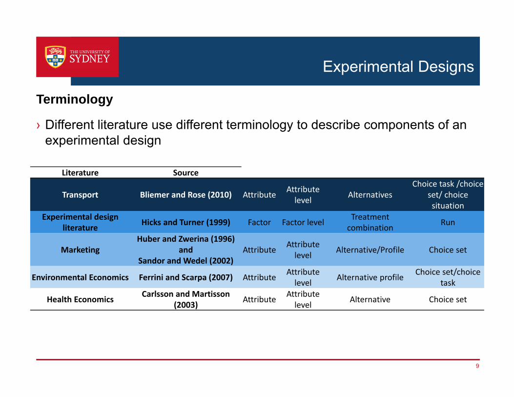
› Different literature use different terminology to describe components of an experimental design

Terminology

9

Literature Source

Transport Bliemer and Rose (2010) Attribute Attribute level Alternatives

Choice task /choice set/ choice situation

Experimental design literature Hicks and Turner (1999) Factor Factor level Treatment

combination Run

MarketingHuber and Zwerina (1996)

and Sandor and Wedel (2002)

Attribute Attribute level Alternative/Profile Choice set

Environmental Economics Ferrini and Scarpa (2007) Attribute Attribute level Alternative profile Choice set/choice

task

Health Economics Carlsson and Martisson(2003) Attribute Attribute

level Alternative Choice set



10

€14 €10

Muscat Riesling

2009 2008

New Zealand Italy

Cost (per bottle)

Grape

Year bottled

Country of Origin

Wine A Wine B None

€12 €14

Pinot Blanc Semillon

2007 2009

France Australia

Cost (per bottle)

Grape

Year bottled

Country of Origin

Wine A Wine B None

€10 €10

Sav. Blanc Riesling

2008 2008

France Italy

Cost (per bottle)

Grape

Year bottled

Country of Origin

Wine A Wine B None

‘None’ or status quo alternatives, whilst important for the design later, have no attribute levels.

Riesl.

Austr.

Semil.

Riesl.

€10

2008

Italy

€14

2009

2008

Italy

Musc.

2009

N.Z.

€12

Pin. Bl.

2007

France

€10

Sa. Bl.

2008

France

€10€14



11

Experimental Design (X)

Each column represents an attribute.Each row represents a choice task.Riesling

Australia

Semillon

Riesling

€14 €10

Muscat

2009 2008

New Zealand Italy

Cost (per bottle)

Grape

Year bottled

Country of Origin

Wine A Wine B

€12 €14

Pinot Blanc

2007 2009

France

Cost (per bottle)

Grape

Year bottled

Country of Origin

Wine A Wine B

€10 €10

Sav. Blanc

2008 2008

France Italy

Cost (per bottle)

Grape

Year bottled

Country of Origin

Wine A Wine B

Cost Grape Year C.O.O

Wine A Wine BCost Grape Year C.O.O

… … … … … … … …

… … … … … … … …

… … … … … … … …

… … … … … … … …

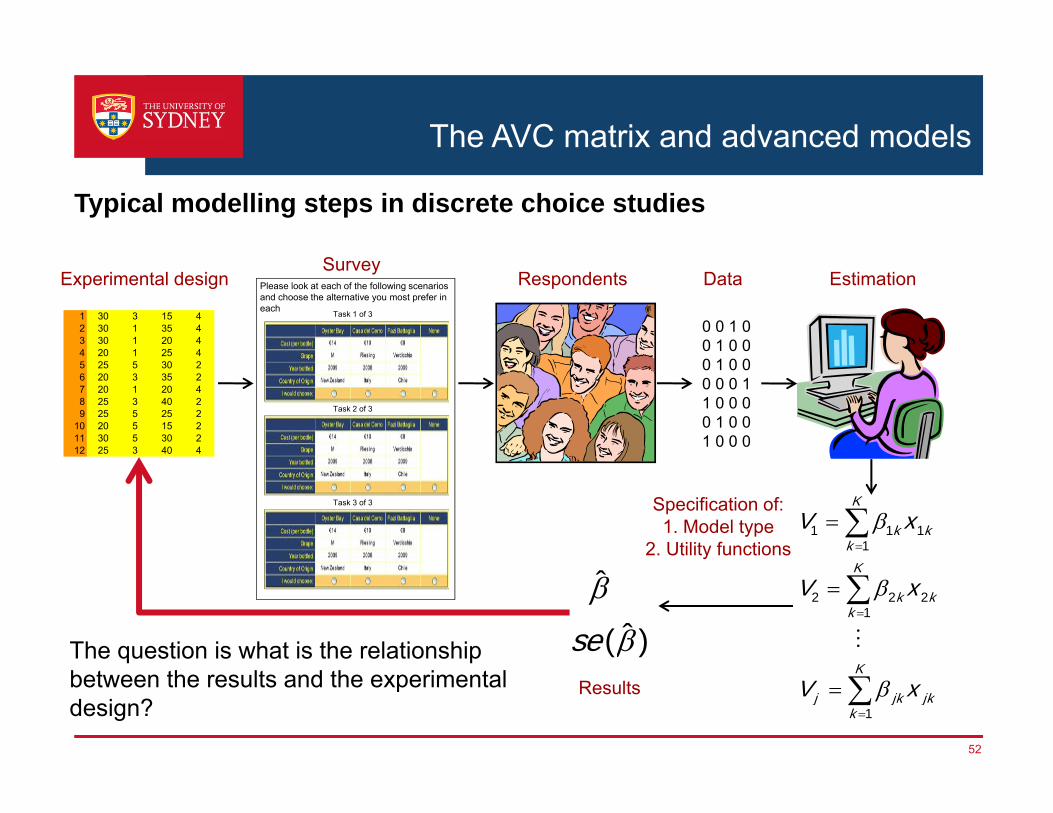
Discrete choice modelling process 2

Discrete choice modelling process

Typical modelling steps in discrete choice studies

13

1 30 3 15 42 30 1 35 43 30 1 20 44 20 1 25 45 25 5 30 26 20 3 35 27 20 1 20 48 25 3 40 29 25 5 25 2

10 20 5 15 211 30 5 30 212 25 3 40 4

0 0 1 00 1 0 00 1 0 00 0 0 11 0 0 00 1 0 01 0 0 0

Task 1 of 3

Task 2 of 3

Task 3 of 3

Please look at each of the following scenarios and choose the alternative you most prefer in each

1 1 11

2 2 21

1

K

k kk

K

k kk

K

j jk jkk

V x

V x

V x

ˆ ˆ( )se

Experimental design Respondents Data EstimationSurvey

Specification of:1. Model type

2. Utility functions

Results

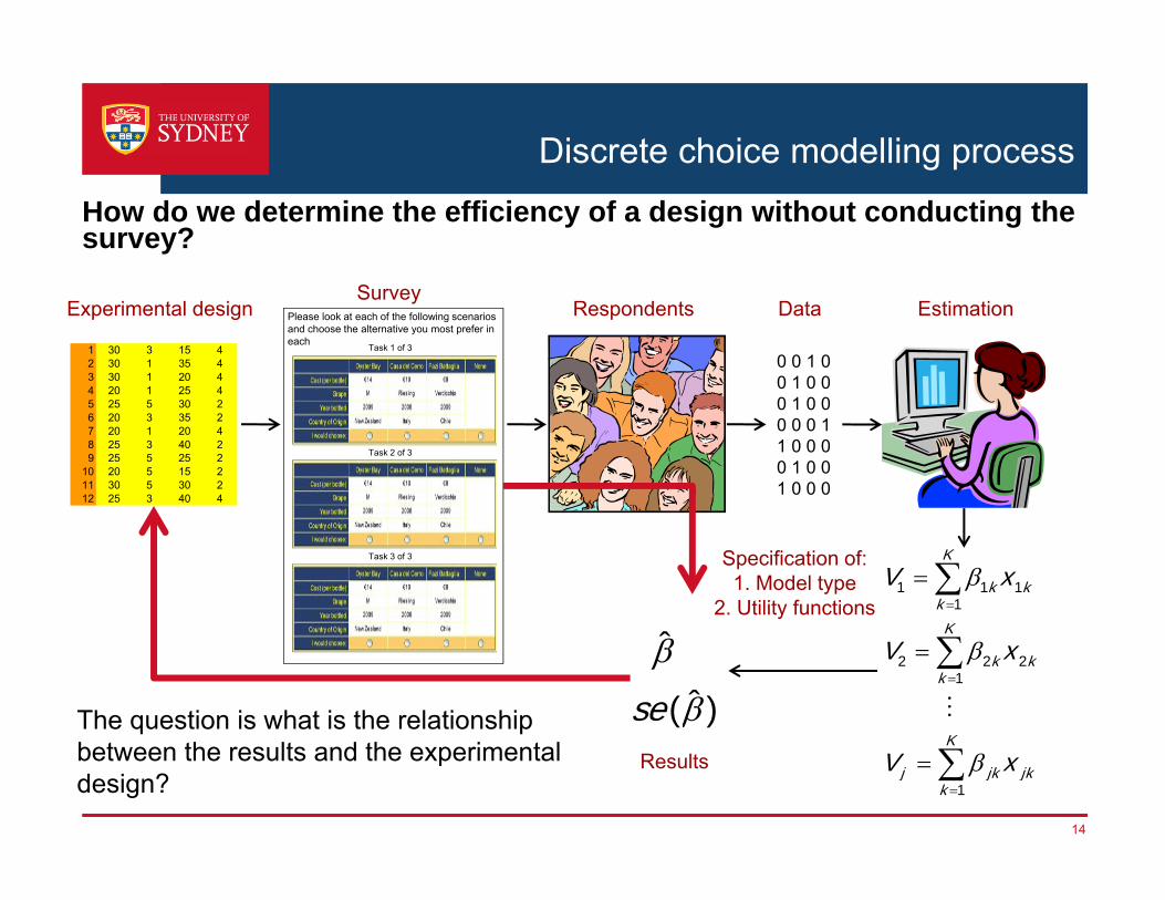
Discrete choice modelling processHow do we determine the efficiency of a design without conducting the survey?

14

1 30 3 15 42 30 1 35 43 30 1 20 44 20 1 25 45 25 5 30 26 20 3 35 27 20 1 20 48 25 3 40 29 25 5 25 2

10 20 5 15 211 30 5 30 212 25 3 40 4

0 0 1 00 1 0 00 1 0 00 0 0 11 0 0 00 1 0 01 0 0 0

Task 1 of 3

Task 2 of 3

Task 3 of 3


1 1 11

2 2 21

1

K

k kk

K

k kk

K

j jk jkk

V x

V x

V x

ˆ ˆ( )se




Results

The question is what is the relationship between the results and the experimental design?

Discrete choice modelling process

› How do we determine the efficiency of a design without conducting the survey?- First, assume prior parameter estimates (best guesses for the true

parameter values)

- Second, approximate the variance-covariance matrix for the parameter estimates - This can be done without conducting any surveys!

To progress....

15

1 30 3 15 42 30 1 35 43 30 1 20 44 20 1 25 45 25 5 30 26 20 3 35 27 20 1 20 48 25 3 40 29 25 5 25 2

10 20 5 15 211 30 5 30 212 25 3 40 4

Experimental design

ˆ ˆ( )se

ˆ ˆ( )se

Asymptotic variance covariance matrix 3

Asymptotic variance covariance matrix

› The asymptotic variance-covariance (AVC) matrix is an approximation of the true variance-covariance matrix

› “Asymptotic” means

- assuming a very large sample; or

- assuming a large number of repetitions using a small sample

› The roots of the diagonals of the variance-covariance matrix denote the standard errors

The A in AVC

17

21

2

( ),

( )K

se

se

variance-covariance matrix where is the standard

error of parameter k( )kse


› First, determine the loglikelihood function:

› Note that:› In estimation, given the (design) data X and the observations y, one aims

to determine estimates such that is maximised [maximum likelihood estimation]

› When generating an experimental design, these parameter estimates are unknown

› The values of depend on the model used (MNL, NL, ML)

Step 1: Log-likelihood function

18

1 1 1( | , ) log ( | )

N S J

N jsn jsnn s j

L X y y P X

( | , )NL X y

( | )jsnP X


› Secondly, determine the Fisher information matrix:

Step 2: Determine the Fisher Information Matrix

19

2 ( | , )( | , )'

NN y

L X yI X y E[expected negativeHessian matrix ofsecond derivatives]


› Note that:- The AVC matrix depends on the design, X

- The AVC matrix depends on the choice observations, y

- The AVC matrix depends on the parameters,

- The AVC matrix depends on the number of respondents, N

› Both y and are unknown when generating a design

Step 3: Determine the AVC Matrix

20

1( | , ) ( | , ) N NX y I X y

!

!

[inverse matrix]


› Example: MNL model with generic parameters (McFadden, 1974)

MNL model AVC

21

1 2 21 1 1 1

( | ) ( | ) ( | )

N S J J

N jk sn jsn jk sn ik sn isnn s j i

I X X P X X X P X

Assuming that all responds observe the same choice situations,

1 2 21 1 1

1

( | ) ( | ) ( | )

( | )

S J J

N jk s js jk s ik s iss j i

I X N X P X X X P X

N I X

1

111

( | ) ( | )

( | )

N N

N

X I X

I X

Therefore, the AVC matrix becomes:

Measuring Efficiency 4

Measuring efficiency

› Numerical Example

Its all about the AVC matrix

23

1 2 1 3 2

2 1 4 2

A

B

U A AU B B

MNL model: Priors: 1

2

3

4

0.20.30.40.5

Design:

1

2

3

4

1 2 3 4

1( | )I X 1( | )X 1

2

3

4

1 2 3 4

10 ( | )X


› Numerical Example

Comparing AVC matrices

24

Design 1:

Design 2:

1

1

Which design is more efficient?


› In order to assess the efficiency of different designs, several efficiency measures have been proposed

› The most widely used ones are:- D-error

- A-error

› The lower the D-error or A-error, the more efficient the design

Its all about the AVC matrix

25

1/1det K

1trK

[determinant of AVC matrix]

[trace of AVC matrix]

K number of parameters (size of the matrix), used as a scaling factor for the efficiency measure


Comparing AVC matrices...

26

Design 1:

Design 2:

1

1

D-error = 0.568A-error = 2.761

D-error = 0.434A-error = 2.194

Design 2 is more efficient


› So, if we know and , then we can compute the t -ratio for any sample size.

› Suppose that a t -ratio of is requested for parameter

› Then the required sample size for this parameter is

› The required overall sample size (for all parameters) is

Optimising sample sizes

27

2*

1 ( )kk

k

se tN

k 1 ( )kse

*t

max kkN N

k


› The property of utility balance is sometimes seen as a requirement for efficiency (Huber and Zwerina, 1996)

- A design is more utility balanced if there are no dominating alternatives in the choice situations

Utility balance I

28

1 2 1 3 2

2 1 4 2

A

B

U A AU B B

1

2

3

4

0.20.30.40.5

• compute UA and UB• compute PA and PB• compute utility balance factor B

0.2 0.3 2 0.4 1 0.80.3 2 0.5 1 1.1

A

B

UU

exp(0.8) / exp(0.8) exp(1.1) 0.43exp(1.1) / exp(0.8) exp(1.1) 0.57

A

B

PP

0.43 0.57 100% 98%0.50 0.50

B


› Numerical Example› General formulation of the utility balance is measure:› Utility balance per choice situation:

P = (½, ½) gives 100%, P = (1,0) gives 0%

P = (⅓, ⅓, ⅓) gives 100%, P = (1,0,0) and P = (½, ½,0) give 0%

› Average utility balance for whole design:

Utility balance II

29

1

100%1/

Jjs

sj

PB

J

1

1 S

ss

B BS

10.23 0.17 0.60 100% 63%0.33 0.33 0.33

B

63% 29% 79% 98% 96% 3% 61%6

B


› The higher utility balance, the better? No!› A 100% utility balanced design will be very inefficient (why?)› A design with a very low utility balance is inefficient too (why?)› What is a good level of utility balance?

- Indication for a design with 2 alternatives: utility balance of 70% – 90%

- This corresponds with probabilities (0.25,0.75) – (0.35,0.65)

- These probabilities are confirmed by so-called “Magic P” values (discussed later)

- More research on this topic needed (especially with respect to designs with more than 2 alternatives)

Utility balance III

30

D-error

utility balance100%50%


› WTP is calculated as the ratio of the change in marginal utility of attribute kto the change in marginal utility for a cost attribute

› Both parameters have standard errors and covariances (which come from the AVC matrix)

› Using the delta method

Willingness to pay

31

k kk k k

cc c

c

d xx dx

dCost xdx

2

2

21. . . ,k

c

k kk k c c

c c c

s e Var Cov Var


› It is therefore possible to minimise the standard errors of the ratios of two parameters (WTP)

› We call this C-error (or WTP-error)

Willingness to pay

32

min max . .k

c

kC error s e

The prior parameters 5

The prior parameters

› Prior parameter estimates can be obtained from:- the literature

- pilot studies

- focus groups

- expert judgement

› If no prior information is available, what to do?

Where can I get my priors?

34

1. Create a design using zero priors or use an orthogonal design

2. Give design to 100% of respondents

1. Create a design using zero priors or use an orthogonal design

2. Give design to 10% of respondents3. Estimate parameters, use as priors4. Create efficient design5. Give design to 90% of respondents


Parameter prior misspecification I

35

› What if the priors have been wrongly specified?› For example, what if is 0.6 instead of 0.4 ?

› The AVC matrices and D-errors for the D-efficient design are:1

1 0.4

1 0.6

D-error = 0.1775

D-error = 0.2074

Designs are efficient under the assumption oftrue parameter values.Wrongly specified priorstypically lead to a loss inefficiency.


Parameter prior misspecification II

36

0.1 0.2 0.3 0.4 0.5 0.6 0.7

0.18

0.2

0.22

0.24

0.26

0.28

0.3

0.32

0.34

0 0.1 0.2 0.3 0.4 0.5 0.6

0.18

0.2

0.22

0.24

0.26

0.28

0.3

0.32

0.34

0 0.1 0.2 0.3 0.4 0.5 0.6

0.18

0.2

0.22

0.24

0.26

0.28

0.3

0.32

0.34

0.3 0.4 0.5 0.6 0.7 0.8 0.9

0.18

0.2

0.22

0.24

0.26

0.28

0.3

0.32

0.34

-1.8 -1.6 -1.4 -1.2 -1 -0.8 -0.6

0.18

0.2

0.22

0.24

0.26

0.28

0.3

0.32

0.34

0.1 0.2 0.3 0.4 0.5 0.6 0.7

0.18

0.2

0.22

0.24

0.26

0.28

0.3

0.32

0.34

0.4 0.5 0.6 0.7 0.8 0.9 1

0.18

0.2

0.22

0.24

0.26

0.28

0.3

0.32

0.34

1 2 3 4

5 6 7

D-error

It is possible to alreadycheck beforehand to which parameters the design is most sensitive to.

One can put more effort in finding good priors for these parameters.

Introduction to Ngene 6

Introduction to Ngene

Experimental design generation software

38

www.choice-metrics.com


design;alts = alt1, alt2, alt3;rows = 8;eff = (mnl,d,fixed);con;model:U(alt1) = b1[1.2] + b2[-0.6]*A[6,8,10,12] + b3[-0.4]*B[4,8] + b4[0.3] *C[0,1] /U(alt2) = b5[0.8] + b2 *A + b3 *B + b6[0.8] *C /U(alt3) = b2 *A + b7[-1.0]*C$

1 11 12 13

2 21 22 23

3 31 33

1.2 0.6 0.4 0.30.8 0.6 0.4 0.8 0.6 1.0

U x x xU x x xU x x

11 21 31

12 22

13 23 33

, , {6,8,10,12},, {4,8}, and, , {0,1}.

x x xx xx x x

39

Example syntax

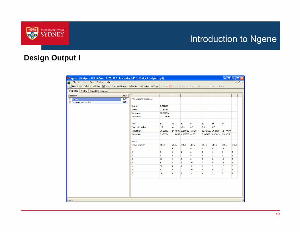
40


Design Output I

Bayesian prior parameter distributions 7

Bayesian prior parameter distributions

› Efficient design- Example:

- Find D-efficient design based on priors

› Bayesian efficient design- Example:

- Find Bayesian D-efficient design based on priors

Background

42

k

2~ ( , )k k kN


Prior parameter distributions

43

k k kkk

kl khk

Pr( )k Pr( )k Pr( )k

2~ ( , )k k kN ~ ( , )k k kU l h=k k Fixed Normal Uniform


› Each efficiency measure (D-error, A-error, etc.) has a Bayesian counterpart (Bayesian D-error, Bayesian A-error, etc.)

› Since the priors are random parameters, the efficiency measures will be random too

› Bayesian efficiency measures the expected efficiency

Bayesian measures I

44

1/det ( | ) KXD-error =

Bayesian D-error =

Example:Using D-efficiency as efficiency measure and assuming 2~ ( , )N

1/ 2det ( | ) ( | , )KX f d

Normal probability density function


› Bayesian efficiency is difficult to compute, it needs to evaluate a complex (multi-dimensional) integral

› However, it is nothing more than a simple average of D-errors:

where are random draws from the distribution function (we take r = 1,…,R draws)

Bayesian measures II

45

Bayesian D-error = 1/det ( | ) ( | )KX f d

Bayesian D-error ≈ 1/( )

1

1 det ( | )R Kr

rX

R

( )r


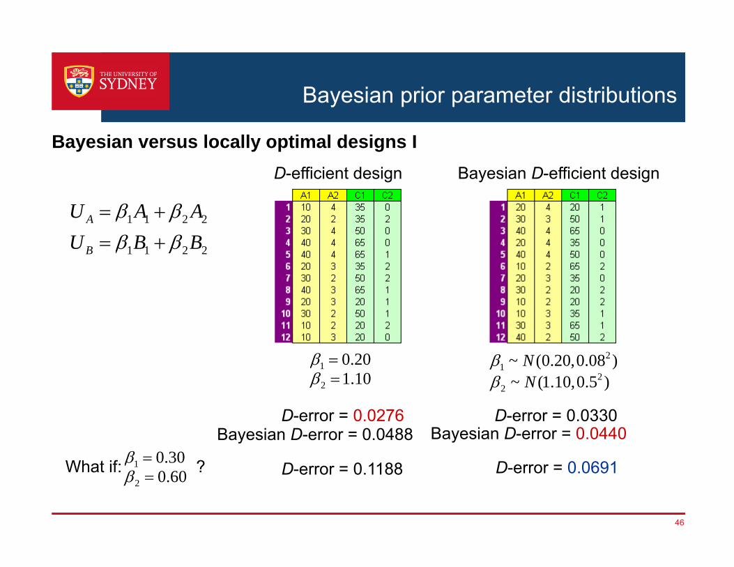
Bayesian versus locally optimal designs I

46

D-efficient design Bayesian D-efficient design

1 1 2 2

1 1 2 2

A

B

U A AU B B

21

22

~ (0.20,0.08 )~ (1.10,0.5 )

NN

1

2

0.201.10

D-error = 0.0276 D-error = 0.0330Bayesian D-error = 0.0488 Bayesian D-error = 0.0440

D-error = 0.1188 D-error = 0.06911

2

0.300.60

What if: ?


› Efficient designs are more efficient than Bayesian efficient designs if the prior parameters are correct

› However, if the priors are wrong, an efficient design can become quite inefficient

› The efficiency of a Bayesian D-efficient design is less sensitive to misspecification of the priors, and therefore called more robust

Bayesian versus locally optimal designs II

47


› The same algorithms for determining an efficient design can be used for generating a Bayesian efficient design

› If R random draws (e.g., 100) are used for computing the Bayesian efficiency, finding a Bayesian efficient design may take R times longer

› It is recommended to always use ‘smart draws’ (e.g., Halton draws) instead of random draws

Generating Bayesian efficient designs

48

49

design;alts = alt1, alt2, alt3;rows = 12;eff = (mnl,d,mean);bdraws = halton(100);con;model:U(alt1) = b1[1.2] + b2[(n,-0.6,0.2)]*A[6,8,10,12] + b3[-0.4]*B[4,8] + b4[0.3] *C[0,1] /U(alt2) = b5[0.8] + b2 *A + b3 *B + b6[0.8] *C /U(alt3) = b2 *A + b7[-1.0]*C$

2 ~ ( 0.6,0.2)N


Example Syntax

50


Interpreting Bayesian output

The AVC matrix and advanced models 8Bliemer, M.C.J. and Rose, J.M. (2010) Construction of Experimental Designs for Mixed Logit Models Allowing for Correlation Across Choice Observations, Transportation Research Part B, 44, 720-734

The AVC matrix and advanced models

Typical modelling steps in discrete choice studies

52

1 30 3 15 42 30 1 35 43 30 1 20 44 20 1 25 45 25 5 30 26 20 3 35 27 20 1 20 48 25 3 40 29 25 5 25 2

10 20 5 15 211 30 5 30 212 25 3 40 4

0 0 1 00 1 0 00 1 0 00 0 0 11 0 0 00 1 0 01 0 0 0

Task 1 of 3

Task 2 of 3

Task 3 of 3


1 1 11

2 2 21

1

K

k kk

K

k kk

K

j jk jkk

V x

V x

V x

ˆ ˆ( )se




Results

The question is what is the relationship between the results and the experimental design?


› The asymptotic variance-covariance (AVC) matrix is an approximation of the true variance-covariance matrix

› “Asymptotic” means

- assuming a very large sample; or

- assuming a large number of repetitions using a small sample

› The roots of the diagonals of the variance-covariance matrix denote the standard errors

Recall...

53

21

2

( ),

( )K

se

se

variance-covariance matrix where is the standard

error of parameter k( )kse




The MNL model

54

1

ln .n ns

N

nsj nsjn s S j J

LL y P

1 2 2

1 2

2* * *

* *1 1n ns

N J

nsjk nsj nsjk nsi nsikn s S j J ik k

LogL x P x P x

1 1 1 1 2 2

1 1 2

2* *

*1 1n ns

N J

j k s j s j k s ik s isn s S j J ij k k

LogL x P x x P

1 1 2 2 1 2

1 1 2 21 1 2 2 1 2

1 221

1 21

, if ;

1 , if .

n ns

n ns

N

j k s j k s j s j sn s S j J

Nj k j k

j k s j k s j s j sn s S j J

x x P P j jLogL

x x P P j j




The cross sectional MMNL model

55

1

ln .n ns

N

nsj nsjn s S j J

LL y E P

1 1 2 2 1 1 2 2 1 1 2 2

22

21

log ( ) 1 1 .n ns

Nnsj nsj nsj

nsjn s S j Jk m k m k m k m k m k mnsj nsj

P P PE L y E E EE P E P

nsjP




The panel MMNL model

56

1

ln | ,nsj

n ns

N y

nsjn s S j J

LL P f d

1 1 2 2 1 1 2 2 1 1 2 2

1 1 2 2 1 1 2 2

2 * * *2

2* *1

2 * * *

2* *1

log ( ) 1 1

1 1 ,

Nn n n

nk m k m k m k m k m k mn n

Nn n n

n k m k m k m k mn n

E P E P E PE LE P E P

P P PE E EE P E P

** ,

n ns

nsj nsjn kn

s S j Jkm km nsj k

y PP PP

1 1 1

1

1 1 2 2 1 1 2 2 1 1 2 2 2 1 1 2 2 1

22 * * ** *

*

1 ,n ns n ns

k k knsj nsj nsjn n nn nsjk n

s S j J s S j Jk m k m n k m k m k m k m k k m k m nsj k

P y PP P P P x PP P

.ns

nsjnsj nsjk nsi nsik

i Jk

PP x P x

where


› Error components models are a form of MMNL models

› They can be therefore also be treated as cross sectional or panel models

Error components models

57

nsj nsj n h nsjU x z d 1 if alt is in nest 0 otherwise. h

i hd

where

and ),0(~ NZn

Design;alts = alt1, alt2, alt3;rows = 20;eff = (rpecpanel,d);rdraws = gauss(2);bdraws = gauss(2);rep = 250;model:

U(alt1) = SP1[0.8] + b1[n,(n,-0.8,0.1),(u,0.1,0.2)] * A[5,10,15,20] + b2[n,1.2,0.2] * B[0,1,2,3] + b3[1.2] * C[0,1,2,3] + b4[-0.7] * D[1,2,3,4] + EC[EC,1] /

U(alt2) = SP2[0.6] + b1 * A + b2 * B + b3 * C + b4 * D + EC $


Bayesian random parameters…

58

Design;alts = alt1, alt2, alt3;rows = 20;eff = (rpecpanel,d);rdraws = gauss(2);bdraws = gauss(2);rep = 250;model:

U(alt1) = SP1[0.8] + b1[n,(n,-0.8,0.1),(u,0.1,0.2)] * A[5,10,15,20] + b2[n,1.2,0.2] * B[0,1,2,3] + b3[1.2] * C[0,1,2,3] + b4[-0.7] * D[1,2,3,4] + EC[EC,1] /

U(alt2) = SP2[0.6] + b1 * A + b2 * B + b3 * C + b4 * D + EC $


Bayesian random parameters…

59

Experimental design influences on stated choice outcomesCase study 1: An empirical study in air travel choice


Bliemer, M.C.J. and Rose, J.M. (2011) Experimental design influences on stated choiceoutputs: an empirical study in air travel choice, Transportation Research Part A, 45(1),63‐79.

Introduction 1

Introduction

› Orthogonal designs have been widely used in stated choice experiments.

› Efficient designs have been proposed to yield smaller standard errors in model estimation.

› Until now, efficient designs have not been compared to orthogonal designs in real life with respect to their standard errors, only in hypothetical simulation studies.

› In this study we investigate whether the theoretical advantages of› efficient designs (smaller standard errors at smaller sample sizes) indeed

translate into practice.

Orthogonal vs. efficient designs

62

Introduction

Empirical studies

63

“More efficient designs lead to greater error variance (lowerscale parameter).” – Louviere et al. (2008)

“Efficient designs only lead to marginal improvements overorthogonal designs, design blocking seems more important.” – Hess et al. (2008)

“Efficient designs can lead to significantly lower standard errors andrequire smaller sample sizes than using an orthogonal design.” – Bliemer and Rose (2010)

Description case study 2

Description case study

› Investigate travel behavior of travelers, depending on: Airline

ticket price

transfers

departure time

egress travel time

egress travel costs

using a web-based stated choice experiment for a trip from Amsterdam to Barcelona.

Air travel choice

65


Barcelona or Girona airport?

66

Amsterdam

Barcelona


Online booking

67


Online booking

68

Experimental design 3

Experimental design

Design dimensions

70

› Alternatives: 5

› Number of choice situations per respondent: 6

› Attributes and levels:

airline: Air France, KLM, Iberia, Vueling, Transavia, EasyJet ticket price: €50, €75, €100 transfer time: none, 1 hour, 2 hours departure time: 6am, noon, 6pm egress travel time: 20min, 30min, 40min (Barcelona)

60min, 80min, 100min (Girona) egress travel costs: €1, €3, €5 (Barcelona)

€9, €12, €15 (Girona)

Experimental design

Design generation (using Ngene)

71

› Three designs have been generated:- orthogonal design

Number of choice situations: 108Number of blocks: 18

- Bayesian D-efficient design 1*Number of choice situations: 108Number of blocks: 18

- Bayesian D-efficient design 2*Number of choice situations: 18Number of blocks: 3

* Using parameter priors from pilot study (36 respondents, orthogonal design)

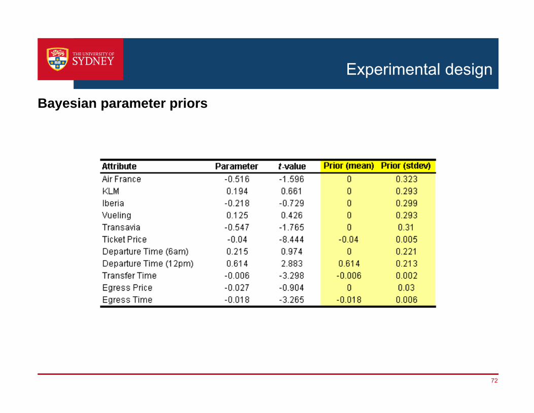
Experimental design

Bayesian parameter priors

72

Experimental design

Efficient design *

73

Model Estimation 4

Model Estimation

Pooled data results (using Nlogit)

75

Attribute parameter t-ratio lower 95% upper 95%

Air France 0.377 6.019 0.254 0.500

KLM -0.232 -3.456 -0.364 -0.101

Iberia -0.535 -7.629 -0.672 -0.398

Vueling -0.008 -0.120 -0.132 0.117

Transavia -0.137 -2.046 -0.268 -0.006

Ticket Price -0.028 -25.115 -0.030 -0.026

Departure Time (6am) 0.283 6.221 0.194 0.372

Departure Time (12pm) 0.460 9.860 0.368 0.551

Transfer Time -0.015 -32.228 -0.016 -0.014

Egress Price -0.035 -5.956 -0.047 -0.024

Egress Time -0.009 -8.459 -0.011 -0.007

Model fits

LL(ASC only model) -5879.526

LL(β) -4774.862

ρ2 0.188

Respondents 618

Observations 3708

“Travellers are willing to pay 10 euros more for a ticket to Barcelona Airport (and save 40 minutes egress time)”

“Travellers are willing to pay 10 euros more for a ticket to Barcelona Airport (and save 40 minutes egress time)”

206 orthogonal design208 efficient design 1204 efficient design 2

Model Estimation

Design-specific results

76

Design 1: Orthogonal, S = 108 Design 2: Efficient, S = 108 Design 3: Efficient, S = 18

Attribute par. t-ratiolower 95%

upper 95% par. t-ratio

lower 95%


lower 95%

upper 95%

Air France 0.422 3.423 0.180 0.664 0.319 2.994 0.110 0.527 0.457 4.401 0.253 0.660

KLM -0.231 -1.883 -0.471 0.010 -0.402 -3.265 -0.643 -0.161 -0.112 -1.017 -0.328 0.104

Iberia -0.488 -3.756 -0.742 -0.233 -0.650 -5.445 -0.884 -0.416 -0.417 -3.523 -0.649 -0.185

Vueling 0.285 2.345 0.047 0.524 -0.141 -1.324 -0.349 0.068 -0.131 -1.173 -0.351 0.088

Transavia 0.024 0.190 -0.227 0.276 -0.301 -2.635 -0.524 -0.077 -0.052 -0.469 -0.270 0.166

Ticket Price -0.035 -17.780 -0.038 -0.031 -0.023 -10.808 -0.027 -0.019 -0.021 -9.649 -0.026 -0.017

Departure Time (6am) 0.300 3.311 0.123 0.478 0.410 5.387 0.261 0.560 0.171 2.285 0.024 0.318

Departure Time (12pm) 0.627 7.181 0.456 0.798 0.348 4.181 0.185 0.511 0.303 3.786 0.146 0.460

Transfer Time -0.011 -13.999 -0.012 -0.009 -0.015 -19.410 -0.017 -0.014 -0.018 -22.350 -0.020 -0.017

Egress Price -0.041 -3.311 -0.065 -0.017 -0.038 -3.894 -0.057 -0.019 -0.032 -3.330 -0.051 -0.013

Egress Time -0.012 -5.205 -0.016 -0.007 -0.006 -3.102 -0.010 -0.002 -0.006 -3.342 -0.01 -0.003

Model fits

LL(ASC only model) -1953.577 -1940.001 -1983.633

LL(β) -1557.904 -1607.444 -1550.317

ρ2 0.203 0.171 0.218

Respondents 206 204 208

Observations 1236 1248 1224

Design comparison 5

Design comparison

Efficient 1 (S=108) vs. Efficient 2 (S=18)

78




lower 95%


lower 95%

upper 95%

Air France 0.422 3.423 0.180 0.664 0.319 2.994 0.110 0.527 0.457 4.401 0.253 0.660

KLM -0.231 -1.883 -0.471 0.010 -0.402 -3.265 -0.643 -0.161 -0.112 -1.017 -0.328 0.104

Iberia -0.488 -3.756 -0.742 -0.233 -0.650 -5.445 -0.884 -0.416 -0.417 -3.523 -0.649 -0.185

Vueling 0.285 2.345 0.047 0.524 -0.141 -1.324 -0.349 0.068 -0.131 -1.173 -0.351 0.088

Transavia 0.024 0.190 -0.227 0.276 -0.301 -2.635 -0.524 -0.077 -0.052 -0.469 -0.270 0.166

Ticket Price -0.035 -17.780 -0.038 -0.031 -0.023 -10.808 -0.027 -0.019 -0.021 -9.649 -0.026 -0.017



Transfer Time -0.011 -13.999 -0.012 -0.009 -0.015 -19.410 -0.017 -0.014 -0.018 -22.350 -0.020 -0.017

Egress Price -0.041 -3.311 -0.065 -0.017 -0.038 -3.894 -0.057 -0.019 -0.032 -3.330 -0.051 -0.013

Egress Time -0.012 -5.205 -0.016 -0.007 -0.006 -3.102 -0.010 -0.002 -0.006 -3.342 -0.01 -0.003

Model fits

LL(ASC only model) -1953.577 -1940.001 -1983.633

LL(β) -1557.904 -1607.444 -1550.317

ρ2 0.203 0.171 0.218



Design comparison

Orthogonal (S=108) vs. Efficient 1 (S=108)

79




lower 95%


lower 95%

upper 95%

Air France 0.422 3.423 0.180 0.664 0.319 2.994 0.110 0.527 0.457 4.401 0.253 0.660

KLM -0.231 -1.883 -0.471 0.010 -0.402 -3.265 -0.643 -0.161 -0.112 -1.017 -0.328 0.104

Iberia -0.488 -3.756 -0.742 -0.233 -0.650 -5.445 -0.884 -0.416 -0.417 -3.523 -0.649 -0.185

Vueling 0.285 2.345 0.047 0.524 -0.141 -1.324 -0.349 0.068 -0.131 -1.173 -0.351 0.088

Transavia 0.024 0.190 -0.227 0.276 -0.301 -2.635 -0.524 -0.077 -0.052 -0.469 -0.270 0.166

Ticket Price -0.035 -17.780 -0.038 -0.031 -0.023 -10.808 -0.027 -0.019 -0.021 -9.649 -0.026 -0.017



Transfer Time -0.011 -13.999 -0.012 -0.009 -0.015 -19.410 -0.017 -0.014 -0.018 -22.350 -0.020 -0.017

Egress Price -0.041 -3.311 -0.065 -0.017 -0.038 -3.894 -0.057 -0.019 -0.032 -3.330 -0.051 -0.013

Egress Time -0.012 -5.205 -0.016 -0.007 -0.006 -3.102 -0.010 -0.002 -0.006 -3.342 -0.01 -0.003

Model fits

LL(ASC only model) -1953.577 -1940.001 -1983.633

LL(β) -1557.904 -1607.444 -1550.317

ρ2 0.203 0.171 0.218



Design comparison

Efficient designs are in practice indeed more efficient;Shows that theoretical efficiency indeed translates into practical efficiency.

Size of the design does not influence efficiency;Shows that small designs are sufficient.

Note: there exists no orthogonal design with S<108.

D-errors of the data sets

80

Orthogonal design (S=108)

D-efficient design 1 (S=108)

D-efficient design 2 (S=18)

D-error 0.1253 0.1035 0.1017

Design comparison

Standard errors (bootstrapped)

81

0 20 40 60 80 100 120 140 160 1800

0.05

0.1

0.15

0.2

0.25

0.3

0.35

0.4

0.45

0.5

0 20 40 60 80 100 120 140 160 1800

0.05

0.1

0.15

0.2

0.25

0.3

0.35

0.4

0.45

0.5

0 20 40 60 80 100 120 140 160 1800

0.05

0.1

0.15

0.2

0.25

0.3

0.35

0.4

0.45

0.5

0 20 40 60 80 100 120 140 160 1800

0.05

0.1

0.15

0.2

0.25

0.3

0.35

0.4

0.45

0.5

0 20 40 60 80 100 120 140 160 1800

0.05

0.1

0.15

0.2

0.25

0.3

0.35

0.4

0.45

0.5

0 20 40 60 80 100 120 140 160 1800

0.005

0.01

0.015

Air France KLM Iberia

Vueling Transavia Ticket Price


Efficient design 1 (S=108)


Design comparison

Standard errors (bootstrapped)

82




Departure 6am Departure 12pm Transfer Time

Egress Price Egress Time

0 20 40 60 80 100 120 140 160 1800

0.05

0.1

0.15

0.2

0.25

0.3

0 20 40 60 80 100 120 140 160 1800

0.05

0.1

0.15

0.2

0.25

0.3

0 20 40 60 80 100 120 140 160 1800

1

2

3

4

5

6

7

8x 10

-3

0 20 40 60 80 100 120 140 160 1800

0.005

0.01

0.015

0.02

0.025

0.03

0.035

0.04

0.045

0.05

0 20 40 60 80 100 120 140 160 1800

1

2

3

4

5

6

7

8

x 10-3

Design comparison

Required sample sizes (bootstrapped)

83

0 50 100 150 200

Air France

KLM

Iberia

Ticket Price

Departure 6am

Departure noon

Transfer Time

Egress Time

Egress Price

sample size

orthogonal (S=108) efficient (S=108) efficient (S=18)

Design comparison

Prediction power of t-ratios

84

0 5 10 15 20 250

5

10

15

20

25

predicted t-ratio

obse

rved

t-ra

tio

orthogonal designefficient design (S=108)efficient design (S=18)

These t-ratios can be usedto obtain indications about

minimum required sample sizes(S-estimates).

These t-ratios can be usedto obtain indications about

minimum required sample sizes(S-estimates).

Conclusions and discussion 6

Conclusions and discussion

› 1. Efficient designs lead in practice to smaller standard errors, as predicted by the theory, thereby outperforming orthogonal designs.

› 2. The size (number of choice situations) of the design has no influence on the efficiency. Hence, there is no need to use large designs. Small orthogonal designs in general do not exist, however efficient designs can be kept very small.

Take away 1 and 2

86


› 3. The S-estimates introduced by Bliemer and Rose (2005,2009) & Rose and Bliemer (2005) seem indeed to offer a good prediction for the required sample sizes for statistically significant parameter estimates.

› 4. Accurate parameter priors used for generating efficient designs are important, efficiency is quickly lost with incorrect priors. Bayesian priors are therefore recommended.

Take away 3 and 4

87


› 5. As also found by Louviere et al. (2008), highly efficient designs yield larger error variance (smaller scale). Less efficient designs (e.g., orthogonal designs) seem to have smaller error variance (larger scale) due to the existence of more dominant alternatives in a choice situation. Therefore, the design can have an influence on the exact parameters due to this scale factor.

› 6. Although in this case study the MNL model was used, the same arguments can be used for other model types (e.g., MMNL).

Take away 5 and 6

88

What’s next?What are we currently working on?


What’s next

› Availability designs- To date, all work in efficient designs has assumed all alternatives are available in

all choice tasks

- Here we allow variable choice set sizes (varying the number of alternatives) either at the discretion of the user or as a variable to optimize on

› Best worst designs- Best worst cases 1,2 and 3 can be set up to be modeled using logit models

- The difference is the data structure

- We are working on optimizing for the unique data structures associated with these question mechanisms

What are we working on…

90

What’s next

› Designs accounting for information processing strategies (IPS)- In generating designs, it is assumed that all attributes will be fully attended to

- A zero prior is not the same as assuming that an attribute will be ignored given that in modeling we would remove an attribute with an insignificant parameter estimate

- Here we add an additional Bayesian which will remove an attribute from the utility function up to a probability

› Designs allowing for non-linear utility functions› New model types including designs for WTP space, latent class

What are we working on…

91

1 2 2

1 2

2

1 1 1 1

( | ) ( | ) ( | )N S J J

Njk sn jsn jk sn ik sn isn

n s j ik k

L X X P X X X P X

Serial Choice Conjoint Analysis for Estimating Discrete Choice ModelsCase study 2: The future????


Bliemer, M.C.J. and Rose, J.M. (2010) Serial Choice Conjoint Analysis for EstimatingDiscrete Choice Models in Hess, S. and Daly, A. (ed.) Choice Modelling: State‐of‐the‐Artand the State‐of Practice: Proceedings from the Inaugural International ChoiceModelling Conference, Emerald Press, Bingley, United Kingdom, 139‐61.

What is a good design? 1

What is a good design?

› yields parameter estimates with high accuracyunbiased, close to true values

› yields parameter estimates with high precisionhigh reliability, low standard errors

A good experimental design

94

What is a good design?

Observation 1:Any experimental design can be used to find the true parameters

[all designs yield accurate parameter estimates… in the limit!]

Observation 2:A ‘good’ experimental design will find these true parameters at (much) smaller sample sizes than ‘bad’ designs;

[a good design yields more precise parameter estimates]

So, how to find these ‘good’ (efficient) experimental designs?

A good experimental design

95

Building good designs 2

Building good designs

Different design types

97

Efficient?

Orthogonal?

Burgess and Street (2003) Street et al. (2001, 2005)Street and Burgess (2004)

Yes No

No

Yes

Louviere et al. (2000)

Bunch et al. (1994)Kuhfeld et al. (1994)Huber and Zwerina (1996)Bliemer and Rose (2006, 2007, 2008)Carlsson and Martinsson (2003)Ferrini and Scarpa (2006)Johnson et al. (2006)Kanninen (2002, 2005)Kessels et al. (2005, 2009)Rose et al. (2008)Sándor and Wedel (2001, 2002, 2005)Toner et al. (1999)Yu et al. (2009)

Other designsOrthogonal designs

D-optimal (efficient)designs based on

0 0


parameterpriors needed


0

Orthogonal designs

0


no parameter priors needed

(assumed zero)


› Priors are best guesses for the unknown parameter values.

› Usually obtained from:

• literature studies

• expert judgment

• pilot studies

Parameter priors

98


Example orthogonal design (zero priors)

99


Example orthogonal design (non-zero priors)

100


› Experimental designs are only efficient under the assumption that the assumed priors are accurate.

› Orthogonal designs assume zero-valued priors.- If the parameters are all zero, why doing the estimation?- Therefore, orthogonal designs will always loose efficiency.

› D-optimal designs assume non-zero valued priors.- If the parameters priors are all accurate, why doing the estimation?- Therefore, D-optimal designs will always loose efficiency.

› How much efficiency is lost?- Depends on how much the actual values deviate from assumed priors.- Approach: create designs in a serial fashion based on current estimates.

Parameter priors

101

Adapt or die… 3

Adapt or die…

› Adaptive designs (such as serial/sequential designs) may be subject to endogeneitybias (Toubia et al., 2003):

“To understand this result we first recognize that any adaptive question-design method is potentially subject to endogeneity bias. Specifically, the qth question depends upon the answers to the first q −1 questions. This means that the qthquestion depends, in part, on any response errors in the first q−1 questions. This is a classical problem, which often leads to bias (see, for example, Judge et al. 1985, p. 571). Thus, adaptivity represents a tradeoff: We get better estimates more quickly, but with the risk of endogeneity bias.”

› Adaptations in the design can happen within-respondent (higher risk of bias)Johnson (1987, 1991), Green et al. (1991)

› across respondents (lower risk of bias)

This presentation

Adaptive designs

103

Adapt or die…

› 1. Initialization• Set n = 1.

• Set priors

› 2. Generate D-optimal design• Find experimental design that minimizes the determinant of the asymptotic variance-covariance

matrix, assuming priors

• Give design to respondent n.

• Observe choices

› 3. Estimate parameters• Use data to obtain maximum likelihood parameter estimates

› 4. Update priors

• Set

Parameter priors

104

.nY

( ) 0.n

nX

( , )n nX Y ( )ˆ .n

( ).n

( )( )

ˆ ,0,

nn k

k

if parameter is statistically significant;otherwise.

Set n:=n+1,return to Step 2.

Adapt or die…

• Designs need to be generated during the survey, requiring a more complex survey process

• Mainly suitable for • CAPI (computer aided personal interviewing)• Internet-based surveys

• Respondents have to be interviewed in a serial manner,› or alternatively (as proposed by Kanninen and others):

• interview 10% of respondents• estimate parameters• generate new efficient design• interview next 10% of respondents• etc.

Disadvantages serial design process

105

Case Study 4

Case study

› In the case study, we use simulation to generate choice observations. We repeat this process 100 times in a Monte Carlo setting.

› Three experimental designs are considered:• Orthogonal design *

• Fixed D-optimal design (based on true parameters) *

• Serial D-optimal design (based on parameter estimates) **

* Generated using Ngene 1.0

** Generated using Matlab implementation

Background

107

Case study

Priors

108

3,373,133

2,362,242,1322

1,351,241,1311

XXVXXXV

XXXV

}1,0{},8,4{},12,10,8,6{ ,3,2,1 jjj XXX

)0.1,8.0,3.0,4.0,6.08.0,2.1(

MNL model with following utility functions:

Attribute levels:

Parameter priors:

Number of choice situations per respondent: 12

Case study

› Compare the following experimental designs:

1. Orthogonal design (no priors needed)

2. Locally D-optimal design, assuming


What was done

109

)(ˆ i

orthogonal design, see Louviere et al. (2000)

efficient design, see Huber and Zwerina (1996)

serial design, this presentation

Case study

Results I

110

0 10 20 30 40 50 60 70-1

0 10 20 30 40 50 60 70-1

0 10 20 30 40 50 60 70-1

n n n

2̂ 2̂ 2̂efficient design orthogonal design serial design

-1

-0.5

0

0.5

1

1.5

2

-1

-0.5

0

0.5

1

1.5

2

-1

-0.5

0

0.5

1

1.5

2

Case study

Results I

111

0 10 20 30 40 50 60 70-1

-0.5

0

0.5

1

1.5

2

0 10 20 30 40 50 60 70-1

0 10 20 30 40 50 60 70-1

0 10 20 30 40 50 60 70-1

n n n


-1

-0.5

0

0.5

1

1.5

2

-1

-0.5

0

0.5

1

1.5

2

-1

-0.5

0

0.5

1

1.5

2

Case study

Results I

112

0 10 20 30 40 50 60 70-1

-0.5

0

0.5

1

1.5

2

0 10 20 30 40 50 60 70-1

-0.5

0

0.5

1

1.5

2

0 10 20 30 40 50 60 70-1

0 10 20 30 40 50 60 70-1

0 10 20 30 40 50 60 70-1

n n n


-1

-0.5

0

0.5

1

1.5

2

-1

-0.5

0

0.5

1

1.5

2

-1

-0.5

0

0.5

1

1.5

2

Case study

Results I

113

0 10 20 30 40 50 60 70-1

0

1

2

0 10 20 30 40 50 60 70-1

-0.5

0

0.5

1

1.5

2

0 10 20 30 40 50 60 70-1

-0.5

0

0.5

1

1.5

2

0 10 20 30 40 50 60 70-1

0 10 20 30 40 50 60 70-1

0 10 20 30 40 50 60 70-1

n n n


-1

-0.5

0

0.5

1

1.5

2

-1

-0.5

0

0.5

1

1.5

2

-1

-0.5

0

0.5

1

1.5

2

Case study

Results II

114

0 10 20 30 40 50 60 70

0.6

0.65

0.7

0.75

0.85

0.9

0.95

1

2ˆ( )E

n

2

efficient design

orthogonal design

serial design

Case study

Results II

115

0 10 20 30 40 50 60 70

0

0.5

1

1.5

2

2.5

3

3.5

n

efficient design

orthogonal design

serial design

t –ratio )/( 22 se

Case study

Results: Expected parameter estimates for different sample sizes

116

0 10 20 30 40 50 60 70

0.9

1

1.1

1.3

1.4

1.5

0 10 20 30 40 50 60 70

0.6

0.65

0.7

0.75

0.85

0.9

0.95

1

0 10 20 30 40 50 60 70

-0.75

-0.7

-0.65

-0.55

-0.5

-0.45

0 10 20 30 40 50 60 70

-0.5

-0.45

-0.35

-0.3

1̂( )E

n

1

2ˆ( )E

3ˆ( )E 4

ˆ( )E n

n n

2

3 4

0 10 20 30 40 50 60 70

0.22

0.24

0.26

0.28

0.32

0.34

0.36

0.38

0 10 20 30 40 50 60 70

0.6

0.65

0.7

0.75

0.85

0.9

0.95

1

0 10 20 30 40 50 60 70-1.3

-1.2

-1.1

-0.9

-0.8

6ˆ( )E

n n

5 6

7ˆ( )E

n

7

efficient design

orthogonal design

serial design

Case study

Results: Expected t -ratios for different sample sizes

117

0 10 20 30 40 50 60 700

1

2

3

4

5

0 10 20 30 40 50 60 700

0.5

1

1.5

2

2.5

3

3.5

0 10 20 30 40 50 60 700

2

4

6

8

10

12

14

16

18

0 10 20 30 40 50 60 700

2

4

6

8

10

n n

3t 4tn n

1t 2t

0 10 20 30 40 50 60 700

0.5

1

1.5

2

0 10 20 30 40 50 60 700

0.5

1

1.5

2

2.5

3

3.5

4

4.5

0 10 20 30 40 50 60 700

1

2

3

4

5

6

n n

n

5t 6t

7t

efficient design

orthogonal design

serial design

Case study

Results: Required sample size for parameter estimation*

118

*N

0

20

40

60

80

100

120

140efficient design

orthogonal design

serial design

*for statistical significance )05.0(

Potential problem? 5

Potential problem?

› Serial designs may lead to biased parameter estimates in small sample sizes

› However, serial designs enable small standard errors (high t-ratios)

› Parameters seem biased in small sample sizes due to (very) bad priors used to generate serial designs for the first few respondents

› Solution: Use orthogonal design for first few respondents, and then generate serial efficient designs

Biases?

120

Potential problem?

› Compare the following experimental designs:

1. Orthogonal design (no priors needed)


3. a) For first 20 respondents: orthogonal design

b) For next respondents: locally D-optimal design, assuming

Case study revisited

121

( )ˆ i

orthogonal design, see Louviere et al. (2000)

efficient design, see Huber and Zwerina (1996)

serial design, see this presentation

Potential problem?

New results

122

0 10 20 30 40 50 60 700

0.5

1

1.5

2

2.5

3

3.5

0 10 20 30 40 50 60 70

0.6

0.65

0.7

0.75

0.85

0.9

0.95

1

2ˆ( )E

n

2

n

2t

efficient design orthogonal design serial design

Conclusions 5

Conclusions

• With a serial design, no predefined priors are required (zero-valued parameter values are assumed), therefore one need not worry about priors misspecification.

• With a serial design, approx. the same level of efficiency can be achieved as with a D-optimal design based on accurate priors.

• Since parameters are estimated continuously, data collection can automatically stop if sufficient respondents have been interviewed.

• Endogeneity bias in small sample sizes can be avoided by using an orthogonal design for the first few respondents.

• Respondents need not be interviewed in a completely serial manner, but can be interviewed in batches.

Summary

124

Documents

Workshop on experimental designs - SDU...Experimental Designs › Exactly how analysts distribute the levels of the design attributes over the course of an experiment (which typically